Conditional Decomposition Discrepancy: Separating Conditional Bias from Sampling Bias in Small-Sample Cross-Domain Cost Forecasting

Abstract

Sample discrepancy measurement is an essential step in transfer learning models such as cross-domain cost forecasting. However, tools that can effectively separate conditional bias from sampling bias are still lacking, so discrepancy information cannot fully support sample screening and model-update decisions. This paper analyzes the information boundary of the maximum mean discrepancy (MMD) in bias attribution, states and proves the relevant propositions, and proposes shifting the object of testing from the joint distribution to the conditional distribution. On this basis, the conditional decomposition discrepancy (CDD) measure is designed: a conditional mean and a residual bandwidth are estimated from an independent calibration sample, the data are projected onto a common residual axis and subjected to a kernel two-sample test, and the test result is converted into a continuous risk score with reference to the permutation null distribution. Numerical experiments are then designed on a UK property transaction price dataset. The results show that, provided the conditional difference is transmitted to the residual marginal, the proposed measure effectively detects conditional bias and reduces the proportion of contaminated source-domain samples under controlled injection, thus offering a new discrepancy measurement tool for data screening in transfer learning.

1. Introduction

Cross-domain forecasting is an important problem at the intersection of applied mathematics and machine learning. In particular, measuring the sample discrepancy between target-domain and source-domain samples is essential for both model training and subsequent maintenance [1]. In cost forecasting, for example, samples from the product under study, the local region, or the recent period must first be gathered as target-domain data for model training. Such data, however, are typically small-sample by nature [2]: usually only tens to a few hundred samples are available, whereas the covariates involve technical condition, production scale, and material and labor costs, among others. A limited amount of source-domain data must therefore be introduced only on the basis of a discrepancy judgment, such as medium- to long-term historical data, data from other fields, or data from similar products. Such approaches are generally classified as transfer learning and, when several source domains are involved, are also referred to as multi-source domain adaptation or multi-source transfer learning [3,4,5,6,7,8].

However, enlarging the sample with source-domain data in order to accelerate model convergence is often accompanied by risks [9]: when the conditional relationship differs between the source and target domains, indiscriminate transfer introduces systematic bias and degrades rather than improves performance in the target domain. A further issue is maintenance after the model is deployed [10,11,12]. As new batches of data keep arriving, if it cannot be determined whether a new batch results from a conditional bias or from a sampling bias caused by input-side noise and other factors, the only options are to leave the model unchanged or to retrain it: the former leads to steadily declining accuracy, whereas the latter wastes computing resources when the data fluctuate within their normal range [13]. The root cause of these problems is the absence of a sample-discrepancy criterion suited to the requirements of this scenario [14]. This paper therefore addresses the small-sample cross-domain cost-forecasting setting and proposes a discrepancy measure that separates conditional bias from sampling bias, providing a criterion for source-domain sample screening and model-update decisions.

2. Related Work

2.1. Taxonomy of Discrepancy Measures

Discrepancy measures admit two standard classification schemes. The first, rooted in probability theory and mathematical statistics, expresses the distance between two probability measures uniformly as an integral probability metric (IPM) and classifies measures by the function class employed; this framework was proposed by Müller (1997) [15] and systematically consolidated by Sriperumbudur et al. (2010) [16]. The second, based on reproducing kernel Hilbert space (RKHS) theory, classifies measures by the space into which the distribution is embedded and by the manner of the embedding; this framework was organized by Berlinet and Thomas-Agnan (2004) [17] and Muandet et al. (2017) [18]. It is compatible with the unified IPM framework and facilitates a class-by-class discussion of sensitivity to changes in the conditional relationship. Under this classification, the common discrepancy measures fall into six classes.

The first class defines difference through functionals of probability densities. It originates from the information theory of Kullback and Leibler (1951) [19], was symmetrized by Lin (1991) into the Jensen–Shannon divergence [20], and was generalized by Csiszár (1967) into f-divergences [21]. Its principle is to gauge the departure of two distributions by the expectation of a density ratio or density difference. Recently, Li et al. (2026) [22] embedded the KL divergence together with a decay factor into the target-task value-function update of transfer reinforcement learning to guide path-planning learning, thereby turning the divergence directly into a learning signal rather than a test statistic; Xu et al. (2026) [23] introduced a KL divergence with a dynamic scaling factor into deep embedded clustering and down-weighted ambiguous samples to preserve local data structure. This class has the advantages of clear interpretation and easy embedding of the divergence into a learning objective, but it requires density estimation or an analytic density. In high-dimensional, small-sample regimes, the estimation error contaminates the metric directly; and when the two distributions have almost disjoint support the metric may be undefined or numerically explosive. In current small-sample multi-domain settings, such methods are therefore usually combined with other learning objectives rather than used alone for nonparametric testing.

The second class characterizes difference by low-order moments, tracing back to the method of moments. Its modern form builds indices from differences in means, covariances, and higher-order moments, projecting distributional difference onto a few statistics and measuring sample discrepancy directly through deviations of those statistics. Tao et al. (2013) [24], for example, constructed a nonparametric difference index that depends only on moments and not on the distributional form, and derived critical values for normal and Pareto populations, yielding a robust and inexpensive discrepancy measure. Such methods are computationally very cheap and need no density estimation, but they are insensitive to changes in distributional shape or in the conditional relationship: under a second-moment criterion, two distributions with identical means and covariances are treated as identical, which discards high-dimensional features such as distributional shape. Current work therefore combines moment-based indices with regularization for robust decision-making and distributionally robust optimization.

The third class defines difference by a supremum over a function class or by a transport cost. Its theoretical origin is optimal transport, and its modern forms include the Wasserstein, Sinkhorn, energy, and Cramér distances, which together form a complete family of distances; the principle is to take the minimum cost of transporting one distribution onto another as the measure of difference. Pereira and Amini (2025) reviewed the theory and algorithms of optimal transport [25], covering duality, entropy regularization, and relaxed formulations, and identified domain adaptation as a principal application. Zeng and Jiang (2026) [26] replaced the conventional cost by an optimized kernel mean discrepancy to build an ensemble transport filter; Chen and Tan (2025) [27] combined paired structure with the energy distance to propose a k-paired-sample test; and Matabuena (2019) [28] combined the energy distance with kernel mean embedding for a two-sample survival test under right censoring. These methods offer clear geometric interpretation and usually avoid density estimation, but their exact solution is expensive and its cost rises sharply with dimension, so they are rarely used in high-dimensional small-sample settings. Current work focuses on entropy-regularized solvers and on the construction of dependence measures.

The fourth class builds test statistics from univariate empirical distribution functions, originating from the two-sample test on empirical distribution functions (the Kolmogorov–Smirnov test) [29] and from the tail-sensitive statistic of Anderson and Darling (1952) [30]. Its principle is to compare the maximum deviation or the weighted squared deviation between two empirical distribution functions. Recently, Linden (2026) extended the Kolmogorov–Smirnov, Cramér–von Mises, and Anderson–Darling statistics to any k weighted samples under a shared permutation inference procedure, noting that the first is most sensitive to centrally located differences while the latter two are more sensitive to tail differences [31]. Pereira and Amini (2025) reviewed the theory and algorithms of optimal transport in machine learning and identified domain adaptation as a principal application [25]. Such methods are nonparametric, have favorable small-sample properties, and are computationally very cheap, but they can only handle one-dimensional or very low-dimensional comparisons. Current work generalizes these statistics to more general sampling designs and high-dimensional projection settings.

The fifth class measures difference through the separability learned by a trained discriminator; it is represented by domain confusion and adversarial domain adaptation, and its principle is to take “whether a discriminator or adversarial neural network can tell two samples apart” as the measure of difference [32]. The representative of this line is deep domain confusion [32], which folds the domain-classifier loss into network training so as to learn domain-invariant features. These methods are highly expressive and can operate directly on high-dimensional raw inputs, but they require training, are unstable in small samples, and return only the scalar of separability, which cannot indicate whether the difference originates on the input side or the conditional side.

The sixth class maps distributions onto the mean elements of a reproducing kernel Hilbert space (RKHS) and defines difference by the distance between mean elements. It is represented by the maximum mean discrepancy (MMD) of Gretton et al. (2012), together with its two distribution-free tests and one test based on the asymptotic distribution [14]. Sriperumbudur et al. (2010) [16] gave the necessary and sufficient condition for the embedding to be injective, which was later shown to metrize weak convergence under a characteristic kernel; Micchelli et al. (2006) [33] had earlier characterized the approximation properties of universal kernels; and Muandet et al. (2017) [18] later systematized the framework into a methodology spanning marginal embeddings, theoretical guarantees, and conditional embeddings. Such methods are now widely used in fault diagnosis, process monitoring, clustering ensembles, and complex-system modeling—structural settings characterized by small samples, multiple source domains, and conditional drift [34,35,36,37,38,39]—and are of considerable practical value.

Among these methods, information-theoretic divergences and discriminative approaches are the most expressive, but the former depends on density estimation and the latter on training, so neither is stable in small samples. Moment-based methods and univariate empirical-distribution tests are the cheapest and behave best in small samples, yet they capture only low-order structure and handle only one-dimensional problems, respectively. The optimal transport family strikes a balance between geometric interpretability and computational cost but remains sensitive to high-dimensional data. In high-dimensional discrepancy measurement with small samples, however, the covariates are often too numerous for density estimation, the sample size too small for training complex discriminators, maintenance decisions still require testable significance, and the consistency of the criterion demands theoretical guarantees. Only the measure defined through kernel mean embedding simultaneously satisfies four properties—being nonparametric, requiring no density estimation, admitting a permutation-constructed null distribution, and metrizing weak convergence—and is therefore preferable in small-sample, unknown-distribution settings where testability is required.

2.2. MMD and Its Improvements

The core idea of MMD is to treat a distribution as a point in an RKHS and to characterize distributional difference by the distance between two such points [14]. Its test statistic can be computed directly from sample averages of the kernel function, and its null distribution can be built by permuting labels, so the test is usable in finite samples. This idea is widely adopted in cross-domain modeling: MMD is embedded as a domain loss in deep networks to align cross-domain feature distributions [8], and it is also used to identify mode switching in process monitoring [40,41]. Classic MMD nevertheless has several shortcomings: the discriminative power of the kernel matrix degrades in high dimension [42], changes in the conditional relationship are diluted by directional averaging in the joint space [43,44], and they are scalarized together with changes in the input distribution, so that the two are difficult to distinguish. Grouped by the object of improvement, existing work on these shortcomings falls into two lines: kernel-type modification, which changes the kernel function or the feature map itself, and combination-form modification, which combines or aggregates multiple kernels, bandwidths, or statistics.

Kernel-type modification rests on the observation that the kernel function determines how the feature map responds to differences, so changing its form may change the sensitivity of the criterion to a particular type of difference. Solak et al. (2003) [45] incorporated function values and partial derivatives jointly into the covariance of a Gaussian process, making the model more sensitive to local variation; Mroueh et al. (2019) [46] combined kernel mean discrepancy with the Sobolev norm to transport the source distribution to the target distribution along the minimum-kinetic-energy path and established corresponding convergence results. Such methods improve the response to specific differences, but within the scope of a fixed linear operator they do not change the object of testing: however the kernel is modified, the criterion still operates on the same base kernel and the same comparison object, and its null hypothesis remains that of the same joint-distribution difference. Other kernel-modification paths may alter the finite-sample power of the test without changing that null-hypothesis object.

Combination-form modification starts from the premise that a single kernel form has inherent defects, and instead of changing the type of one kernel, it combines or aggregates multiple kernels, bandwidths, or statistics so as to cover different scales or viewpoints. Its representatives are multiple-kernel MMD, optimally aggregated kernel MMD, and median-heuristic-bandwidth MMD [47]. Gretton et al. [47] selected the kernel parameters that maximize power at a given significance level; Long et al. (2015) [8] used multiple-kernel selection in a domain-adaptation network to align feature distributions across domains; and the median heuristic chooses the bandwidth adaptively from the scale of the samples. These methods are effective for small- and medium-scale testing at a controllable implementation cost, but their gains come from compromise across scales or from merging viewpoints, and they still return a single scalar over the joint distribution: no matter how the kernels, bandwidths, or statistics are combined, they cannot indicate whether the difference originates on the input side or the conditional side.

In summary, existing work on improving MMD either focuses on the kernel function or modifies how kernels and statistics are combined, and in all cases the object of testing is the joint distribution. When the signal of conditional bias is diluted by averaging in the joint space, changing the kernel form or the way kernels and statistics are combined cannot restore the attribution information.

3. Maximum Mean Discrepancy: Principles and Limitations

3.1. Kernel Mean Embedding and the Maximum Mean Discrepancy

Let the input space be X, and let k: X × X → $\mathbb{R}$ be a symmetric positive definite kernel. By the Moore–Aronszajn theorem, there exists a unique reproducing kernel Hilbert space H_k and a feature map ϕ: X → H_k such that

$$\begin{array}{cccc}& k(x,x^{\prime })=⟨\mathrm{\phi }\left(x\right),\mathrm{\phi }\left(x^{\prime }\right){⟩}_{{\mathcal{H}}_k}& & \end{array}$$

(1)

In Equation (1), ${⟨\cdot ,\cdot ⟩}_{H_k}$ is the inner product on H_k, and ϕ maps inputs to elements of H_k. The theorem also yields the reproducing property: for any f ∈ H_k and x ∈ X, $f\left(x\right)={⟨f,k(\cdot ,x)⟩}_{H_k}$; that is, the value of a function at x can be recovered from its inner product with the kernel.

For a probability measure P, its kernel mean embedding is defined as the expectation of the feature map under P.

$$\begin{array}{cccc}& {\mu }_P={\mathbb{E}}_{X\sim P}\left[\varphi \left(X\right)\right]& & \end{array}$$

(2)

In Equation (2), μ_P is an element of H_k. The expectation exists provided that ${\mathbb{E}}_P\left[\sqrt{k(X,X)}\right]<\infty$; when the kernel is bounded (for example, the Gaussian kernel k ≤ 1), this condition holds automatically. By the properties of the Bochner integral, for any bounded linear operator T, we have $\mathbb{E}$[Tϕ(X)] = T$\mathbb{E}$[ϕ(X)]; that is, the expectation commutes with the operator.

Kernel mean embedding maps a distribution to an element of the reproducing kernel Hilbert space (RKHS), and the difference between two distributions can be measured by the distance between their embeddings. Equivalently, taking the unit ball of H_k as the function class $F=\left\{f\in H_k: \parallel f{\parallel }_{H_k} \le 1\right\}$, the maximum mean discrepancy (MMD) between two distributions P and Q is defined as the supremum over this function class of the difference between the two expectations.

$$\begin{array}{cccc}& \mathrm{MMD}(F,P,Q)=\underset{f\in F}{\sup }\left({\mathbb{E}}_P\left[f\left(X\right)\right]-{\mathbb{E}}_Q\left[f\left(Y\right)\right]\right)& & \end{array}$$

(3)

In Equation (3), sup denotes the maximum over the function class; the statistic therefore measures the expectation difference of the unit function that differs most between the two distributions. This definition was given by Gretton et al. (2012), who also noted that it is an instance of an integral probability metric [14]. When the unit ball of H_k is taken, the supremum in Equation (3) has a closed form. For any g ∈ H_k, take $f_g={⟨g,\cdot ⟩}_{H_k}$; when $\parallel g{\parallel }_{H_k} \le 1$, the supremum is attained at $g=\left({\mu }_P-{\mu }_Q\right)/\parallel {\mu }_P-{\mu }_Q{\parallel }_{H_k}$, hence

$${\mathrm{MMD}}^2(P,Q) = \parallel {\mu }_P-{\mu }_Q{\parallel }_{H_k}^2$$

(4)

In Equation (4), $\parallel \cdot {\parallel }_{H_k}$ is the norm in the reproducing kernel Hilbert space. This expression converts the supremum over a function class into the norm of the embedding difference, so that MMD can be computed without explicitly solving a function optimization. By the bilinearity of the inner product, Equation (4) can be further expanded into an expectation form of the kernel.

$$\begin{array}{cccc}& {\mathrm{MMD}}^2(P,Q)=\mathbb{E}\left[k(X,X^{\prime })\right]+\mathbb{E}\left[k(Y,Y^{\prime })\right]-2\mathbb{E}\left[k(X,Y)\right]& & \end{array}$$

(5)

In Equation (5), X,X′ is i.i.d. from P and Y,Y′ is i.i.d. from Q. The rightmost expression depends only on expectations of the kernel and therefore requires no density estimation. Given samples ${\left\{x_i\right\}}_{i=1}^m$ and ${\left\{y_j\right\}}_{j=1}^n$, using the sample average of Equation (5) directly would include the diagonal terms i = j and bias the estimator, whereas removing the diagonal terms yields the unbiased statistic U.

$$\begin{array}{c}{\widehat{\mathrm{MMD}}}_u^2={\displaystyle \frac{1}{m\left(m-1\right)}}{\displaystyle \sum _{\underset{i\ne j}{i,j=1}}^m}k(x_i,x_j)+{\displaystyle \frac{1}{n\left(n-1\right)}}{\displaystyle \sum _{\underset{i\ne j}{i,j=1}}^n}k(y_i,y_j)-{\displaystyle \frac{2}{\mathit{mn}}}{\displaystyle \sum _{i,j}}k(x_i,y_j)\end{array}$$

(6)

where i = 1, …, m and j = 1, …, n. In Equation (6), m and n are the sizes of the two samples, and Gretton et al. [14] proved $\mathbb{E}\left[{\widehat{\mathrm{MMD}}}_u^2\right]={\mathrm{MMD}}^2(P,Q)$; that is, the statistic U is unbiased. Under the null hypothesis that the two batches are identically distributed, the sample labels are exchangeable; therefore, permuting the m + n labels at random B times and recomputing Equation (6) each time yields the empirical null distribution of the statistic. Writing the observed value as ${\widehat{\mathrm{MMD}}}_u^2$, the permutation p-value is

$$\begin{array}{cccc}& p={\displaystyle \frac{1+\#\{b:{\mathrm{MMD}}_{u,b}^2\ge {\mathrm{MMD}}_u^2\}}{B+1}}& & \end{array}$$

(7)

In Equation (7), ${\widehat{\mathrm{MMD}}}_{u,\left(b\right)}^2$ is the statistic recomputed after the b-th relabelling, B is the number of relabellings, and # denotes cardinality; one is added to both the numerator and the denominator so that the p-value is never zero. The exactness of the permutation test and its asymptotic robustness in finite samples were proved by Hoeffding (1952) and by Chung and Romano (2013), respectively [48,49].

Whether MMD being zero is equivalent to the two distributions being identical is addressed by the following theorem.

Theorem 1

(MMD embedding injectivity and weak-convergence consistency). Let (X, d) be a compact metric space and k: X × X → $\mathbb{R}$ continuous and bounded. (i) If k is a characteristic kernel, then for any Borel probability measures P, Q,

MMD_k(P, Q) = 0 ⟺ P = Q.

(ii) If, in addition, k is a universal kernel (equivalently, its RKHS is dense in C(X)), then for any sequence of probability measures {P_n} (in particular, a sequence of empirical distributions),

MMD_k(P_n, P) → 0 ⟺ P_n converges weakly to P.

Among these results, the injectivity of characteristic kernels and the fact that MMD metrizes weak convergence under universal kernels were given by Sriperumbudur et al. [16], and the kernel approximation property by Micchelli et al. [33]. The first conclusion of the theorem shows that MMD can serve as a criterion, and the second shows that the topology induced by MMD coincides with weak convergence, thus providing the basis for the consistency of the test. Both conclusions, however, are asymptotic: with finite samples the actual detection capability of MMD is still constrained by the contrast between signal concentration and noise. A more fundamental limitation is that MMD can hardly distinguish sampling bias from conditional bias and therefore cannot provide a flexible decision criterion for data selection in transfer learning. Taking cross-domain cost forecasting as an example, differences between data from different domains have two sources: first, a change in the input distribution P(x), namely sampling bias, such as a change in batch composition, region or statistical scope; second, a change in the conditions that constitute the cost mechanism, namely conditional bias. The two differ as follows: for sampling bias, the input distribution P(x) changes while the conditional relationship P(y|x) remains unchanged; for conditional bias, the conditional distribution P(y|x) changes, including changes in the conditional mean, conditional variance, higher-order conditional moments and conditional support. In general, sampling bias can be absorbed by recalibrating the output layer, whereas conditional bias implies that the mapping from cost drivers to cost has changed and may require adjusting the model structure. Treating the two alike may bring a risk of negative transfer if conditional bias is tolerated too leniently, or lead to insufficient usable training data if the threshold for sampling bias is too strict. The following subsections give two limitation propositions for MMD and its improved methods in this setting.

3.2. Reweighting Property of the Fixed Bounded Linear Kernel Modification

Let T: H_k → H_k be a fixed bounded linear operator independent of the data distribution; the modified kernel is defined as

$$\begin{array}{cccc}& k_T(z,z^{\prime })=⟨T\mathrm{\phi }\left(z\right),T\mathrm{\phi }\left(z^{\prime }\right){⟩}_{H_k}& & \end{array}$$

(8)

In Equation (8), z = (x, y) is a sample in the joint space and T is a bounded linear operator within the same RKHS, representing a linear modification of the feature map (such as a change in basis or spectral weighting). The essential idea of this construction is sample reweighting in the RKHS, whose representative is kernel mean matching (KMM) [50]: by assigning weights to source-domain samples, the weighted source mean in the RKHS is made as close as possible to the target-domain distribution. This reweighting idea was later widely borrowed in kernel-modification studies of MMD. Kernel modification, however, is in essence a change in how weights are allocated to the same difference vector on the same base kernel, and it cannot provide new information about the attribution of sample differences.

Proposition 1

(reweighting property of the fixed bounded linear kernel modification). Let the difference vector be Δ = μ_P − μ_Q. For a fixed bounded linear operator T, under the modification of Equation (8) the statistic satisfies

$${\mathrm{MMD}}_T^2(P,Q) = \parallel T\left({\mu }_P-{\mu }_Q\right){\parallel }_{H_k}^2 = \parallel T\Delta {\parallel }_{H_k}^2$$

(9)

In Equation (9), Δ is the difference between the two mean embeddings and TΔ is the linear image of the same difference vector; the equality shows that the modified statistic depends only on T and the same Δ. If T is injective, then ${\mathrm{MMD}}_T^2=0\hspace{1em}⟺\hspace{1em}\Delta =0$, and the object of testing is the same as that of classical MMD; if T is not injective, then ${\mathrm{MMD}}_T^2=0$ is equivalent only to TΔ = 0, the null hypothesis is relaxed, and information may be lost.

Proof. 

The proof has four steps.

Step 1: k_T is the inner-product kernel of Tϕ: by the symmetry and positive definiteness of the inner product, k_T(z, z′) = k_T(z′, z), and for any coefficients {c_i},

$$\begin{array}{cccc}& {\displaystyle \sum _{i,j}}{c}_i{c}_j{k}_T(z_i,z_j)={\parallel {\displaystyle \sum _i}{c}_i\mathit{T\varphi }\left(z_i\right)\parallel }^2\ge 0& & \end{array}$$

(10)

Hence k_T is symmetric positive semi-definite.

Step 2: since T is bounded, and by the properties of the Bochner integral, the expectation commutes with T, that is,

$$\begin{array}{cccc}& {\mu }_P^T={\mathbb{E}}_P\left[\mathit{T\varphi }\left(X\right)\right]=T{\mu }_P& & \end{array}$$

(11)

The same holds for Q.

Step 3: for any g ∈ H_k, take $f_g={⟨g,\cdot ⟩}_{H_k}$; then

$$\begin{array}{cccc}& E_P\left[f_g\left(\mathit{T\varphi }\left(X\right)\right)\right]-E_Q\left[f_g\left(\mathit{T\varphi }\left(X\right)\right)\right]={⟨g,T\left({\mu }_P-{\mu }_Q\right)⟩}_{H_k}={⟨g,T\Delta ⟩}_{H_k}.& & \end{array}$$

(12)

Take the supremum of the right-hand side of Equation (12) with respect to g over $\parallel g{\parallel }_{H_k} \le 1$. By the Cauchy–Schwarz inequality, when TΔ ≠ 0, the supremum is attained at $g=T\Delta /\parallel T\Delta {\parallel }_{H_k}$ and equals $\parallel T\Delta {\parallel }_{H_k}$; when TΔ = 0, ${⟨g,T\Delta ⟩}_{H_k}=0$ and the supremum is 0, in which case the identity to be proved in Proposition 1 degenerates to 0 = 0 and holds automatically.

Step 4: since T is bounded, T^∗T is a self-adjoint positive operator, so Equation (9) can also be written as the quadratic form

$$\begin{array}{cccc}& {\mathrm{MMD}}_T^2={⟨\Delta ,T^{\ast }T\Delta ⟩}_{H_k}& & \end{array}$$

(13)

This shows that the entire effect of the modification is embodied in the weights T^∗T. The four steps show that the whole effect of the modification reduces to a reallocation of weights, and Proposition 1 is thereby proved. □

If T is further assumed to be a Hilbert–Schmidt operator (in which case T*T is a compact self-adjoint positive operator), then T^*T can be spectrally decomposed; taking an orthonormal eigenbasis {e_i} with eigenvalues λ_i ≥ 0, and expanding Δ as $\Delta ={\displaystyle {\sum }_i}{a}_i{e}_i$, we obtain

$$\begin{array}{cccc}& {\mathrm{MMD}}_T^2={\displaystyle \sum _i}{\lambda }_i{a}_i^2& & \end{array}$$

(14)

In Equation (14), a_i is the coefficient of the difference vector along the i-th eigendirection and λ_i is the weight assigned to that direction. The proposition shows that, within the scope of a fixed linear operator, kernel modification does not change the null-hypothesis object of the test; although it does not exclude non-linear kernel improvements such as data-dependent kernels and adaptive-bandwidth kernels, it makes clear that kernel-type modification has an inherent deficiency, namely, that it only improves the sensitivity to the same difference and cannot restore attribution information.

3.3. Non-Identifiability of Bias Attribution in Combination-Form Modification

Proposition 1 shows that linear modification within the same base kernel does not change the object of testing, but says nothing about the effectiveness of combining kernels, bandwidths or statistics. This question is equivalent to asking whether, if the kernel or its hyperparameters are tuned to be optimal, the criterion can support attribution of sample differences. To answer it, take the base distribution P = N(0, I₂) and a Gaussian kernel k (with squared bandwidth 1), and construct two contrast distributions: let the variables of the joint distribution be (x, y), where x is the input side and y the target quantity, and let the two changes act on x and on y|x, respectively. The first is a pure input-side shift, with shift a

$$\begin{array}{cccc}& Q_A=N({(a,0)}^{\top },I_2)& & \end{array}$$

(15)

That is, the input distribution changes while the conditional relationship is unchanged;

The second is a pure conditional-side scale change, with scale parameter c

$$\begin{array}{cccc}& Q_B=N(0,\mathrm{diag}(1,c^2))& & \end{array}$$

(16)

That is, the input distribution is unchanged while the conditional relationship changes.

Let Z ∼ N(m₁, Σ₁) and Z′ ∼ N(m₂, Σ₂), and write m = m₁ − m₂ and Σ = Σ₁ + Σ₂; then W = Z − Z′∼N(m, Σ₁ + Σ₂). For Gaussian distributions and a Gaussian kernel, this property yields closed-form expressions for the two MMD values.

Proposition 2

(non-identifiability of bias attribution in combination-form modification). There exists a family of distribution pairs for which the maximum mean discrepancy takes the same value although the required treatments are opposite.

Proof. 

Directly from the Gaussian integral we obtain

$$\begin{array}{cccc}& {\mathrm{MMD}}^2(P,Q_A)={\displaystyle \frac{2}{3}}\left(1-e^{-a^2/6}\right),{\mathrm{MMD}}^2(P,Q_B)={\displaystyle \frac{1}{3}}+{\displaystyle \frac{1}{\sqrt{3\left(1+2c^2\right)}}}-{\displaystyle \frac{2}{\sqrt{3\left(2+c^2\right)}}}& & \end{array}$$

(17)

In Equation (17), a is the input-side shift and c² is the factor by which the conditional noise variance is amplified relative to the baseline; both expressions are closed-form and can be computed directly for given parameters.

From Equation (17), when a → ∞, MMD²(P, Q_A) → 2/3; when c² → ∞, MMD²(P, Q_B) → 1/3. The two increase monotonically in a and c², respectively, and their ranges intersect in (0, 1/3); therefore, for any MMD value v ∈ (0, 1/3) there exists a pair of parameters (a, c²) for which both sides attain the same value v, which constitutes a family of counterexamples. In particular, taking c² = 2 gives

$$\begin{array}{cccc}& {\mathrm{MMD}}^2(P,Q_B)=0.014182,& & \end{array}$$

(18)

Solving Equation (17) backwards for a = 0.3592 so that MMD²(P, Q_A) = 0.014182, the two coincide digit for digit, and Proposition 2 is proved. □

Proposition 2 shows that MMD and its scalar combination forms, however the kernels, bandwidths or statistics are combined, still output a single scalar over the joint distribution, so the attribution of a difference cannot be decided from that value alone. The proposition does not deny the value of combination-form modification for joint-distribution testing; it points out that such modification likewise takes the scalar difference over the joint distribution as its object of testing and cannot provide reliable information for bias-attribution decisions. The conclusion is restricted to scalar combination forms; whether the attribution information can be recovered by arranging the MMD values of several kernels into a vector depends on whether the responses of these kernels to sampling bias and to conditional bias point in different directions, which is beyond the scope of this paper and is not pursued here.

4. Conditional Decomposition Discrepancy: Principles and Advantages

4.1. Principle of the Conditional Decomposition Discrepancy

Propositions 1 and 2 show that, whether kernel-type modification or combination-form modification of MMD is adopted, the object of testing remains unchanged in the joint distribution space, so that the criterion can hardly distinguish whether a difference arises from sampling bias or from conditional bias. This paper therefore designs a discrepancy measure oriented to conditional decomposition, namely the conditional decomposition discrepancy (CDD): a reference mean surface independently calibrated on a small target-domain sample serves as a common benchmark; each batch is projected onto a common residual axis and the kernel two-sample test statistic of the residual marginal distribution is taken as the discrepancy measure. Unlike typical MMD and its improved methods, CDD moves the object of testing from the joint distribution to the residual marginal obtained by projecting the conditional distribution; it neither requires pointwise estimation of the conditional operator nor loses the difference information carried by the residuals, and it avoids the dilution effect of the difference in the high-dimensional joint distribution space.

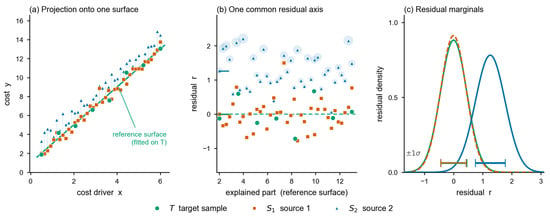
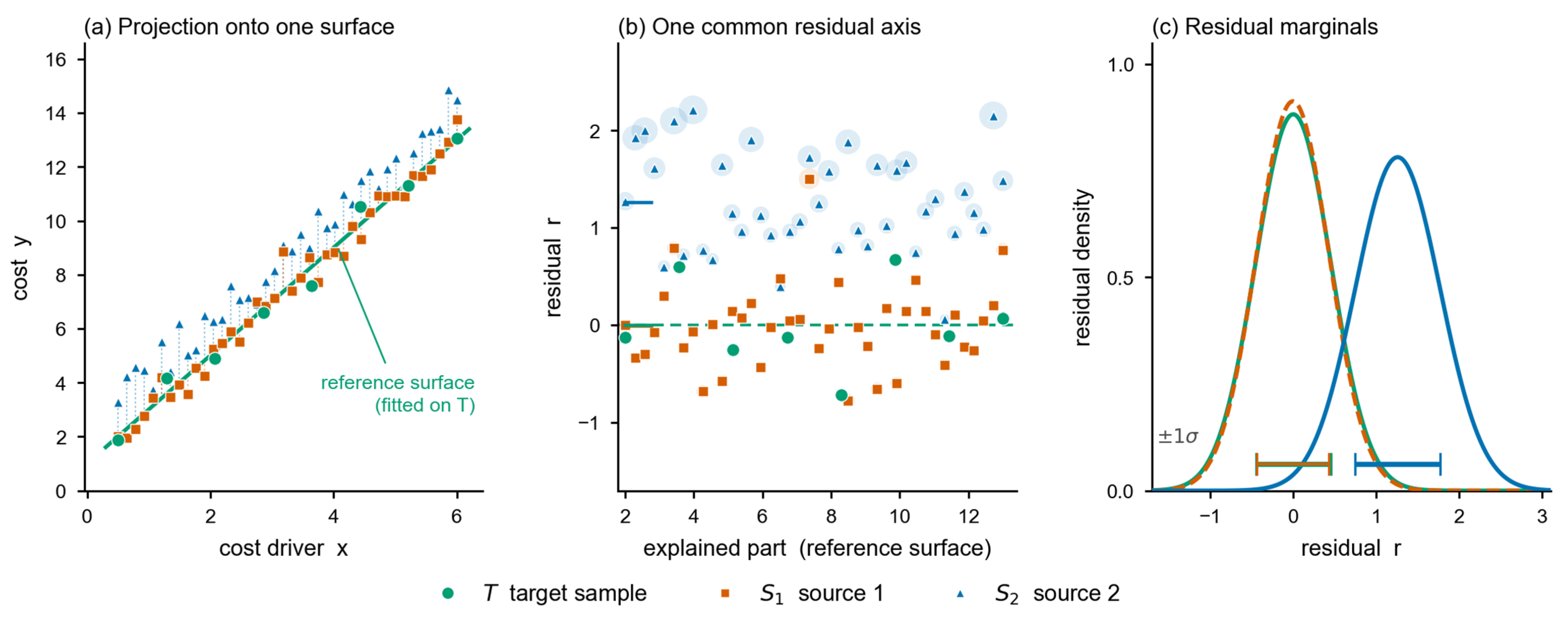
The object of testing of CDD is the residual marginal distribution, so the conditional bias that CDD can detect is limited to the part that remains observable on the residual marginal: when the conditional difference cancels out after mixing at the input side and does not change the residual marginal distribution, CDD stays silent in accordance with Proposition 3, which is both its boundary and the source of its reduced false alarms. The residualisation projection of CDD is shown in Figure 1.

Figure 1. Schematic of the CDD residualisation projection. (a) The reference mean surface $\widehat{m}$_T(x) is fitted on the target-domain calibration samples; (b) source-domain batches are projected onto the residual axis along the same reference surface, giving the residuals r = y − $\widehat{m}$_T(x); (c) a kernel two-sample test is performed on the residual marginal, and the batch-level risk score s is given by the permutation null distribution.

The construction of CDD can be summarized in three steps.

First, a reference mean surface ${\widehat{m}}_T\left(x\right)$ is independently calibrated on a small target-domain sample and serves as a common benchmark for all batches. If each batch estimated its own conditional mean surface, the residuals of each batch would spread around its own fitted surface, the residuals would no longer lie in the same coordinate system, the permutation null distribution would lose its common comparison benchmark, and the risk scores of different batches would not be directly comparable. This paper therefore fixes the reference surface to the common reference surface ${\widehat{m}}_T\left(x\right)$ independently calibrated on the target-domain small sample (which does not take part in fitting the inspected batches), so that the residuals of all batches lie in the same coordinate system, the permutation null distribution has a common benchmark, and comparisons between batches have a consistent reference.

Second, the target domain T and each source-domain batch are projected onto this reference surface, giving their respective residuals:

$$\begin{array}{cccc}& r=y-{\widehat{m}}_T\left(x\right)& & \end{array}$$

(19)

Since all batches share the same reference surface ${\widehat{m}}_T\left(x\right)$, the residuals of different batches are comparable in the same coordinate system. The residual bandwidth ${\widehat{\sigma }}_T$ is estimated from the target-domain calibration samples and then held fixed during permutation, which guarantees the exactness of the permutation null distribution.

Finally, for each pair consisting of the target domain and one source-domain batch, a kernel two-sample test is performed on the residuals. Writing the target-domain residual marginal as ρ^T and the residual marginal of source-domain batch S_i as ${\rho }^{S_i}$, the statistic ${\widehat{\mathrm{MMD}}}_k^2({\rho }^T,{\rho }^{S_i})$ is computed from the unbiased estimator of MMD, Equation (6); the null distribution is then constructed by the MMD permutation procedure, and the standardized risk score is obtained as

$$\begin{array}{cccc}& s_i={\displaystyle \frac{{\widehat{\mathrm{MMD}}}_k^2({\rho }^T,{\rho }^{S_i})-{\mathbb{E}}_{H_0}\left[{\widehat{\mathrm{MMD}}}_k^2\right]}{\sqrt{{\mathrm{Var}}_{H_0}\left({\widehat{\mathrm{MMD}}}_k^2\right)}}}& & \end{array}$$

(20)

In Equation (20), $E_{H_0}$ and ${\mathrm{Var}}_{H_0}$ are the mean and variance under the null distribution, and H₀ denotes the permutation null distribution of the residual labels. s_i is the standardized risk score, used for comparison and ranking across batches; no threshold is set on s_i for the decision; instead, a permutation test is performed separately for each source-domain batch: if the permutation p-value p_i < α, the null hypothesis that this batch and the target domain have identical residual distributions is rejected. For a single batch, CDD therefore gives the scalar risk score s_i of Equation (20); for multiple batches, it outputs the sequence (s₁, …, s_m) of batch-level risk scores, which supports batch-level ranking and screening. The silence and sensitivity propositions of CDD are given and proved below.

4.2. Silence Property of the CDD

Proposition 3

(silence property of the CDD). Suppose the two batches have identical conditional distributions, that is, P(y∣x) = Q(y∣x); the reference model m_T is correctly specified as the conditional mean shared by the two domains; and the residuals are independent and identically distributed given the input-side value, that is, the residual distribution does not depend on the input-side value. Then for any input-side distributions P(x) and Q(x), the corresponding residual marginals ρ^P and ρ^Q satisfy:

$$\begin{array}{cccc}& {\mathrm{MMD}}_k^2({\rho }^P,{\rho }^Q)=0,& & \end{array}$$

(21)

That is, the criterion does not raise an alarm.

Proof. 

Under the assumption that the residuals are independent and identically distributed, the conditional distribution has the form of a location family: given the input-side value x, the conditional distribution of the target quantity equals the distribution of m_T(x) + ϵ, where ϵ has distribution ν, which is independent of x and identical in the two batches; a correct reference model means that m_T is the true conditional mean for both batches. Hence, for any bounded measurable function g,

$$\begin{array}{cccc}& E\left[g\left(Y-m_T\left(X\right)\right)\mid X=x\right]=\int g\left(ϵ\right)\hspace{0.17em}\nu \left(\mathit{dϵ}\right).& & \end{array}$$

(22)

Equation (22) holds for every x, and its right-hand side is independent of x. Therefore, provided the conditional distributions are identical, the residual marginals of the two batches both equal ν, regardless of whether the input-side distributions coincide, that is, ρ^P = ρ^Q. By Theorem 1, ${\mathrm{MMD}}_k^2({\rho }^P,{\rho }^Q)=0$, the population statistic falls within the null hypothesis, and the criterion does not raise an alarm. This completes the proof. □

Three premises are required for the silence property to hold: identical conditional distributions, a correctly specified reference model, and residuals that are identically distributed given the input-side value. The first two are part of the definition of the criterion’s target, whereas the third is an independent assumption: transferability only requires the conditional distributions of the two domains to be identical or similar and does not guarantee that the residuals are identically distributed given the input-side value. In deployment, if the residual distribution keeps changing with the input-side value, the homoscedasticity premise does not hold; the silence property then does not apply, and the criterion may respond to input-side changes. It should be noted that the silence property above holds strictly only under the ideal conditions of a correctly specified reference model and identically distributed residuals. With finite samples, the reference mean surface ${\widehat{m}}_T$ is estimated from the target-domain calibration samples, and its estimation error makes the source-domain residuals deviate from the target-domain residuals, so that the silence property weakens from strictly holding to approximately holding, the degree of approximation depending on the calibration sample size.

4.3. Sensitivity of the CDD

Proposition 4

(sensitivity of the CDD). Let the first batch be the target domain P and the second batch the source domain Q. The conditional distributions of the two batches are not identical, that is, P(y∣x) ≠ Q(y∣x), and this difference is transmitted to the residual marginal (that is, ρ^P ≠ ρ^Q). Then the population statistic is strictly positive; moreover, the alarm probability tends to 1 as the sample size grows.

The transmissibility condition commonly takes two forms: first, the mean channel E_X∼Q[m_Q(X) − m_T(X)] ≠ 0; second, the variance channel, where the conditional variance differs in some input region and both batches have support in that region. Here m_T is the reference conditional mean and m_Q is the conditional mean of the source domain; the expectation is taken with respect to Q_X.

Proof. 

The proof has two steps. In the first step, the difference between the conditional distributions is converted into strict positivity of the population statistic. Let ρ^P ≠ ρ^Q. If the kernel k is characteristic, the kernel mean embedding is injective, and the embedding distance between two distributions is zero if and only if the two distributions are identical; hence

$$\begin{array}{cccc}& {\mathrm{MMD}}_k^2({\rho }^P,{\rho }^Q)>0.& & \end{array}$$

(23)

Equation (23) shows that, provided the transmissibility condition holds, the population statistic is necessarily strictly positive; this conclusion depends only on the injectivity of the characteristic kernel and is independent of the specific kernel form, the bandwidth value and the way the criterion is implemented.

In the second step, population positivity is carried over to the consistency of the test. Writing $\theta ={\mathrm{MMD}}_k^2({\rho }^P,{\rho }^Q)$, the unbiased statistic $\widehat{\theta }$ converges in probability to θ; the null-distribution quantiles converge in distribution to a finite constant when the residual bandwidth is fixed. Under the alternative, the numerator of the standardized score has a constant bias θ and its denominator is of order (m + n)^−1/2, so the score grows at the same rate as $\theta \sqrt{m+n}$ under the alternative. For any significance level α ∈ (0,1), we have

$$\begin{array}{cccc}& \underset{m,n\to \infty }{\lim }\underset{H_1}{\mathrm{Pr}}\hspace{0.17em}\left[s\ge q_{1-\alpha }\right]=1,& & \end{array}$$

(24)

Here m and n are the sample sizes of the two batches, and q_1−α is the upper α-quantile of the permutation null distribution. Equation (24) shows that, provided the conditional difference is indeed transmitted to the residual marginal, the alarm probability of the criterion tends to 1 as the sample size grows. This completes the proof. □

It should be pointed out that the residual-marginal mapping P(y∣x) ↦ P(r) is many-to-one: when the projection of the conditional difference onto the residual marginal is approximately zero, a single-interface CDD stays silent. A feasible way to reduce this risk is to construct multiple residual interfaces, for example, by fitting separate reference mean surfaces with different feature subsets, different basis functions or different regularization schemes, then computing CDD separately on each residual marginal and carrying out a joint decision to recover part of the information about the conditional change. This treatment turns the choice of the reference surface from a fixed premise of the criterion into an adjustable modeling degree of freedom. Owing to space limitations, this paper discusses only the single-interface CDD; the properties and the joint threshold of multi-interface CDD are not developed. The sensitivity proposition states that, when the conditional relationships differ, the criterion can detect the difference and its detection ability increases with the sample size. The premise of the sensitivity direction is the transmissibility condition, that is, the difference between the conditional distributions must be reflected on the residual marginal.

5. Experiments

5.1. Experimental Design and Overall Conclusions

Of the four propositions proposed in this paper, Propositions 1 and 2 have been completely proved, whereas Propositions 3 and 4 have been proved only under given conditions. To show that the conditions under which Propositions 3 and 4 hold cover common application scenarios, a numerical simulation is carried out below with multi-source cross-domain cost forecasting as an example. The experiment uses the property transaction price dataset published by HM Land Registry (HM Land Registry Price Paid Data); the data are divided into 106 classes by postcode district, the PE district, whose data are relatively stable, is taken as the target domain, and 15 relatively complete groups of data are selected from the remaining classes as the source domains. To fully cover the conditions involved in the propositions, the experiment combines real data with controlled simulation: the real-data experiment is mainly used to identify the differences between MMD and CDD in their response to bias, whereas the controlled simulation is mainly used to vary systematically the type and magnitude of bias under known ground truth and to analyze the conditional dependence of Propositions 3 and 4.

First, the alarm rates of MMD and CDD under different drift magnitudes are examined by controlled simulation. Five types of cells, A, B, C, D and E, are designed, corresponding to no change, pure input-side drift, conditional mean drift, conditional scale drift and covariate coefficient drift, respectively; Δ is the magnitude of the change in the conditional relationship, measured in log-price units, and takes five levels, 0, 0.30, 0.80, 1.20 and 1.60. For each cell, the table gives the alarm rates of MMD and CDD; the higher the alarm rate, the more readily the criterion judges that “a difference exists” under the conditions of that cell. The results are given in Table 1.

Table 1. Alarm rates under different drift magnitudes; each cell gives MMD/CDD.

Cell	Setup	Δ = 0	0.30	0.80	1.20	1.60
A. No change	The two batches are identical	0.05/0.07	0.05/0.05	0.05/0.03	0.03/0.07	0.02/0.04
B. Pure input-side drift	Input composition and continuous-dimension means shifted; conditional relationship unchanged	0.04/0.04	0.59/0.06	1.00/0.14	1.00/0.17	1.00/0.18
C. Conditional mean drift	Conditional mean shifted on the dwelling-type D subgroup (share about 30%)	0.05/0.04	0.13/0.15	0.46/0.56	0.79/0.89	0.92/0.97
D. Conditional scale drift	Residual scale enlarged by a factor of 1 + Δ	0.05/0.04	0.09/0.23	0.41/0.99	0.84/1.00	0.97/1.00
E. Covariate coefficient drift	Coefficients of a few dimensions changed	0.03/0.04	0.10/0.19	0.61/0.71	0.91/0.95	0.99/0.99

Note: The values in the table are the alarm rates of the criteria for the corresponding controlled cell and drift magnitude; each cell uses 150 repetitions with 200 label permutations each, at a significance level of 0.05; Cell A is the no-change control cell, used to check the nominal level; 300 re-checks give the Wilson 95% confidence intervals of CDD: 0.883 (0.842–0.915) for Cell C at Δ = 1.20, 0.987 (0.966–0.995) for Cell D at Δ = 0.80, and 0.933 (0.899–0.956) for Cell E at Δ = 1.20.

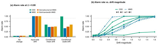
The controlled simulation results show that, in Cell A, the alarm rates of the two criteria both lie near the nominal level (the Type I error rate is set to 5%), indicating that the criteria do not raise false alarms when there is no bias. In Cell B at Δ = 0.80, the MMD alarm rate is 1.00 whereas that of CDD is only 0.14, indicating that under sampling bias MMD is more sensitive than CDD. The CDD alarm rates in Cells C, D and E rise with Δ: at Δ = 0.80 Cell D already reaches 0.99, and at Δ = 1.20 Cell C reaches 0.89 and Cell E 0.95, indicating that under conditional bias CDD is more sensitive than MMD. Figure 2 further shows the response trends of the four criteria: CDD rises steadily with the drift magnitude in the conditional-bias cells and remains low in the pure input-side drift cell, whereas MMD and its improved methods rise rapidly to 1.00 in the pure input-side drift cell and rise slowly in the conditional-bias cells. This trend intuitively supports the properties that CDD is silent to sampling bias and sensitive to conditional bias; Propositions 3 and 4 are thus preliminarily supported.

Figure 2. Alarm rates of the controlled cells. (a) Alarm rates of the four criteria at drift magnitude Δ = 0.80 in the four cells of no change, pure input-side drift, conditional mean drift and conditional scale drift; (b) variation in the alarm rate with drift magnitude Δ in the four cells of pure input-side drift, conditional mean drift, conditional scale drift and covariate coefficient drift. The dotted lines are the 0.05 and 0.90 reference lines; each cell uses 150 repetitions with 200 label permutations each.

5.2. Comparative Experiment on Bias Identification Capability

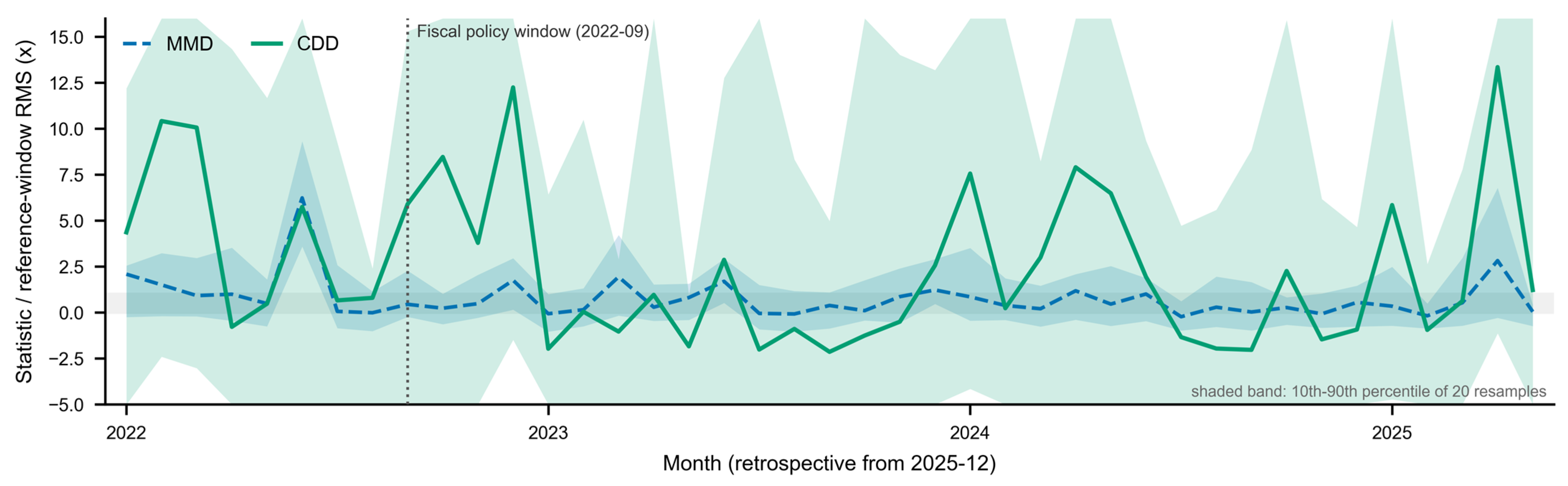
The response differences between CDD and MMD in bias identification are examined below. The experiment is designed as follows: the PE district is taken as the identification district; June 2025 to December 2025 is taken as the reference window, and the full sample of that window is used to fit the reference mean surface and estimate the residual bandwidth; the samples from January 2022 to May 2025 are taken as the objects of inspection, and the two statistics MMD and CDD are computed month by month. To eliminate the dimensional difference between the two statistics, the vertical axis is unified as the ratio obtained by dividing the statistic by the root mean square of the null-hypothesis fluctuation of the reference window; each month the raw statistic is computed from the full sample, and 20 resamplings of 150 samples are additionally used to give the 10th–90th percentile band, which characterizes the within-batch sampling fluctuation. By comparing the response patterns of MMD and CDD over the same period, this experiment examines whether the two criteria exhibit different directions of bias identification on real data. It should be pointed out that, because real data carry no ground-truth labels of bias type and the monthly bias readings are affected by within-batch sampling, this section is an exploratory analysis and does not serve as statistical evidence for Propositions 3 and 4.

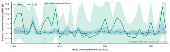
Figure 3 presents the bias response curves of MMD and CDD in the monthly tests for the PE district, where the dashed line is MMD, the solid line is CDD, and the shaded region is the 10th–90th percentile band obtained from 20 resamplings of 150 samples each month, reflecting the range of within-batch sampling fluctuation. It can be seen that the MMD curve stays close to the reference level throughout and shows no obvious response between January 2022 and May 2025. The CDD curve, by contrast, conveys more difference information: during the period from September 2022 to June 2023, the monthly median of CDD is 1.92 times the reference-window fluctuation, whereas in the remaining periods it is 0.23 times, which may be related to the “Mini-Budget” policy window in the United Kingdom in September 2022. In addition, CDD shows two peaks, in December 2022 and October 2022, of 12.25 times and 8.46 times, respectively, suggesting conditional differences between the sample data around the policy window and the benchmark (the period from June 2025 to December 2025). The above descriptive comparison suggests that CDD captured, in the real data over several periods, a relative elevation that MMD could hardly detect, which is broadly consistent with the design expectation that CDD is sensitive to conditional bias.

Figure 3. Bias response curves of MMD and CDD (PE district).

5.3. Comparative Experiment on Screening Capability and Accuracy

The screening capability of each criterion under controlled injection conditions and how it propagates to prediction accuracy are examined below. The experiment is designed as follows: from the 120 batches split out of the 15 source-domain datasets, 40 batches are selected by systematic sampling and injected with perturbations at two strength levels, 0.4 and 0.8 (in natural-log price); the injection is applied only to the conditional mean of the dwelling-type D subgroup, while the input-side distribution is kept unchanged; the calibration set and the evaluation set are district-disjoint, and the 40 batches of the first 5 districts are used to calibrate the thresholds, while the remaining 80 batches of the other 10 districts are used for evaluation. The harm indicator is defined as the harm increment of a batch to the model: training on all batches is taken as the baseline, single batches are then removed one by one and the model is retrained, and the difference in RMSE on the harm evaluation period (January 2026 to February 2026) before and after removal is taken as the harm increment of that batch. If the RMSE decreases after removal, the batch is harmful and the increment is recorded as a positive value; if the RMSE increases after removal, the batch is beneficial and the increment is recorded as a negative value.

Each criterion screens the source batches in ascending order of its own risk score, and the accepted batches together with the local prior are used to train the forecasting model; the model adopts a linear regression architecture, extracts feature vectors from discrete attributes such as tenure type, new-build status and rental status, incorporates interaction terms and regional price index features, and outputs point forecasts of log price through least-squares regression. Evaluation is performed on the test period (March 2026 to June 2026); the primary metric is the aggregation-level log RMSE, obtained by first aggregating the predicted and actual values into “month × dwelling-type” cells and then computing the root mean square error at the cell level, which reduces the effect of noise and helps to identify differences between methods; the auxiliary metrics include the contamination rate (number of accepted drifting batches/number of accepted batches), the number of accepted batches and the aggregation-level hit rate. The screening threshold of each criterion is first determined and frozen on the district-disjoint calibration set (the 40 batches of the first 5 districts) and then applied to the evaluation set (the 80 batches of the remaining 10 districts); the 30 random seeds correspond to repeated subsampling of 150 samples from the source-domain batches, while the selection of injected batches, the injection strength and the division into calibration and evaluation districts are held fixed across seeds.

This experiment is used to test whether the sensitivity advantage of CDD over MMD can propagate from the sample-screening level to the prediction-accuracy level; only three classes are compared, namely the MMD criterion family, CDD and cascaded CDD–MMD. The experimental results are shown in Table 2.

Table 2. Main comparison results (30 random seeds).

Metric	No Screening	Standard MMD	Multi-Bandwidth MMD	Derivative-Kernel MMD	Cascaded CDD–MMD	CDD-Only
Accepted batches	80.0	68.6	68.7	68.7	29.6	36.8
Contamination rate	0.325	0.327	0.313	0.323	0.043	0.077
Aggregation-level RMSE	0.2224 ± 0.0155	0.2079 ± 0.0154	0.2051 ± 0.0159	0.2073 ± 0.0153	0.1575 ± 0.0200	0.1833 ± 0.0227
Aggregation level ±5%	43.0	34.6	35.7	35.0	37.2	41.5
Aggregation level ±10%	62.6	62.2	61.7	61.9	62.2	63.9

Note: The number of accepted batches is the number of source-domain batches entering training; the contamination rate (number of accepted drifting batches/number of accepted batches) is the proportion of injected batches among the accepted batches; the value after the aggregation-level log RMSE is the standard deviation; ±5% and ±10% are aggregation-level hit rates (%); the values in each column are the mean over 30 random seeds, and the value after the RMSE is the corresponding standard deviation. The risk scores are standardized by the mean and variance of the permutation of null distribution; the screening thresholds are determined from quantiles of the risk scores on the calibration set and then frozen.

Paired differences over the 30 seeds are analyzed by bootstrap (2000 resamples) and the Wilcoxon signed-rank test, with multiple comparisons corrected by the Benjamini–Hochberg method. Compared with the no-screening arm, cascaded CDD–MMD has an aggregation-level RMSE lower by 0.065 (95% CI 0.057–0.072) and a contamination rate lower by 0.282 (0.270–0.293), with adjusted p < 0.001; the six RMSE and contamination comparisons against the three MMD criteria are likewise significant (adjusted p < 0.001). The ±5% hit rate is on average 5.7 percentage points lower (raw p = 0.034; after correction across four comparison arms × 4 metrics, q = 0.060), and the ±10% difference is not significant (q = 0.65). Table 2 further shows that the no-screening arm accepts all 80 source-domain batches and has both the highest contamination rate and the highest aggregation-level RMSE; the contamination rates of the three MMD criteria are close and their RMSE improvement is limited; cascaded CDD–MMD has the lowest contamination rate and the lowest aggregation-level RMSE; CDD-only lies between the MMD criterion family and cascaded CDD–MMD. These results indicate that CDD can restrict contaminated source-domain samples from entering training and reduce the influence of harmful batches on the model.

5.4. Parameter Sensitivity and Boundary Experiments

Although the screening experiment shows that CDD can reduce the contamination rate of source-domain samples under the given experimental conditions, the parameter sensitivity of this conclusion and the boundaries within which it holds still require further examination. This section therefore designs a parameter-sensitivity experiment and a boundary experiment: the sensitivity experiment mainly examines the performance of each criterion when parameters such as the magnitude of the conditional-relationship drift δ (δ = 0 denotes identical conditional distributions), the input dimensionality d, the batch size n and the forced acceptance count k are varied; the boundary experiment mainly examines the response of the criteria under four boundary conditions, namely reference-surface misspecification, reference-surface misfit, conditional heteroscedasticity and dilution of the conditional difference.

The sensitivity experiment consists of three groups. The first group is a one-factor-at-a-time comparison: only one experimental parameter in δ, d, or n is changed at a time, and the alarm rates of all five criteria are measured. The second group is a reference-surface coverage experiment, carried out for CDD only, to test the effect of the reference surface (and of the residual interface it induces) on the blind spot of CDD. The coverage rate λ controls the tilt of the reference surface along the X₀ direction (the first component of the input vector): at λ = 0, the reference surface is flat along X₀ and does not follow that direction at all; as λ increases, the tilt along that direction grows proportionally and the coverage of the reference surface in that direction increases. max(0.1, 0.3) denotes fitting two reference surfaces with these two coverage rates, standardizing each by its permutation null distribution and taking the successive maximum, and then performing a permutation test on that maximum; comparing the power of the three reference surfaces and of their combination reveals how the degree of reference-surface coverage mitigates the blind spot of CDD. The third group is a forced-acceptance experiment: 40 batches are selected from the 80 real evaluation batches and injected with perturbations of different strengths, and the cumulative contamination strength k = 40/50/60 of each criterion is compared under a fixed forced acceptance count S(k), so as to test how well the criteria rank risks when contaminated samples are forcibly accepted; this is a stress test.

The boundary experiment examines four conditions. The first is reference-surface misspecification: a quadratic term $\gamma \left(X_4^2-1\right)$ that the reference surface does not contain is added when the data are generated, while the reference surface is still fitted with a linear model; γ = 0/0.25/0.5/1, where γ = 0 denotes correct specification. The null arm is shifted by 0.5 along X₄ (the fifth component of the input vector); this shift exposes the misspecification of the reference surface and does not change the conditional distributions of the two domains; the alternative arm takes a conditional-relationship drift of δ = 0.8 without any input-side shift. The main table reports the results at a calibration sample size of 300, and a calibration sample size of 600 is taken for comparison, to show whether increasing the calibration sample can push the Type I error rate back to the nominal level. The second is reference-surface misfit: the reference surface is fitted only on the target-domain calibration samples, and the source domain under test is shifted by X₄ along dx = 0.5/1.0/1.5/2.0, so that it deviates from the fitting range of the reference surface; this tests whether extrapolation failure is mistaken for a conditional difference. The third is conditional heteroscedasticity: the noise scale varies with the input, σ(x) = σ₀(1 + 0.8∣x₀∣), and the source domain under test simultaneously undergoes a shift of X₄ along dx = 0.5, 1.0, 1.5, 2.0; under the null hypothesis the conditional distributions of the two domains are identical, and the test examines whether the criteria raise false alarms because of variance heterogeneity. The fourth is dilution of the conditional difference: samples of proportion X₀ are selected in descending order of q (q = 1.0, 0.5, 0.2, 0.05), and the conditional-relationship drift δ = 0.8 acts only on the selected samples, to test the detection capability of each criterion when the conditional difference appears in only a few samples.

The design of the parameter-sensitivity and boundary experiments is given in full in Table 3.

Table 3. Design of the parameter-sensitivity and boundary experiments.

Group	Factor	Levels	Default	Metric
One-factor comparison	drift magnitude δ	0/0.5/0.8	0.8	alarm rate (δ = 0 gives the Type I error rate)
	input dimensionality d	10/15/20	10	alarm rate
	batch size n	40/60/80	80	alarm rate
Reference-surface coverage	coverage rate λ	0/0.1/0.3/max	—	alarm rate (200 samples per batch)
Forced acceptance	acceptance count k	40/50/60	—	cumulative contamination strength S(k)
Boundary	misspecification γ	0/0.25/0.5/1	—	Type I error rate, power (CDD)
	misfit dx	0.5/1.0/1.5/2.0	—	alarm rate (five criteria)
	heteroscedasticity dx	0.5/1.0/1.5/2.0	—	alarm rate (five criteria)
	dilution q	1.0/0.5/0.2/0.05	—	alarm rate (five criteria)

Note: Each level of the one-factor, reference-surface coverage and boundary groups uses 300 repetitions with 200 label permutations; the forced-acceptance group uses 30 random seeds with 100 permutations. All alarm rates are evaluated at a significance level of α = 0.05.

Five criteria are compared: MMD, multi-bandwidth MMD, derivative-kernel MMD, CDD and the conditional mean embedding (CME). CME is a kernel-modification method oriented to the conditional distribution: it characterizes the conditional distribution by a conditional mean embedding operator and compares the distance between the conditional embeddings of the two domains in the reproducing kernel Hilbert space, which differs markedly from the CDD approach of leaving the kernel form unchanged and moving the object of testing to the residual marginal obtained by projecting the conditional distribution.

It should be pointed out that the computational complexity of CME is about O(n²d + Kn³ + Bn²), far higher than O(n²d + Bn²) for MMD and O(Bn² + nd²) for CDD; in addition, CME requires inverting an n × n kernel matrix, whose condition number deteriorates easily in high-dimensional small-sample settings and causes numerical instability, so CME is generally not used for batch-wise conditional tests in such settings. Because CME models the conditional distribution directly and is sensitive to differences in conditional means, however, it is still used here as a comparison baseline, in order to compare CDD with conditional-distribution kernel modifications; this is not a comprehensive comparison of the two families.

The experimental results are shown in Table 4.

Table 4. Results of the parameter-sensitivity experiments.

Factor	Level	MMD	Multi-Bandwidth MMD	Derivative-Kernel MMD	CDD	CME
δ	0	0.033	0.043	0.037	0.053	0.060
δ	0.5	0.053	0.067	0.067	0.560	0.410
δ	0.8 (default)	0.063	0.140	0.083	0.907	0.787
d	10 (default)	0.063	0.140	0.083	0.907	0.787
d	15	0.037	0.083	0.037	0.860	0.770
d	20	0.067	0.077	0.060	0.813	0.797
n	40	0.073	0.083	0.073	0.440	0.493
n	60	0.047	0.080	0.053	0.713	0.647
n	80 (default)	0.063	0.140	0.083	0.907	0.787
λ	0/0.1/0.3/max	—	—	—	0.040/0.093/0.683/0.657	—
S(k)	k = 40	5.88	4.04	5.55	4.13	1.47
S(k)	k = 50	8.92	7.34	8.75	6.84	4.01
S(k)	k = 60	13.23	12.23	13.08	10.85	8.69

Note: The values in the table are alarm rates (α = 0.05); in the λ row the cells give the results for λ = 0, 0.1, 0.3 and max (0.1, 0.3) in turn; the S(k) rows give the cumulative contamination strength (0–24, the smaller the better; the expectations under random ordering are 12, 15 and 18, respectively).

Table 4 shows that the magnitude of the conditional-relationship drift δ is an important factor affecting the performance of each criterion: at δ = 0.8 the CDD alarm rate reaches 0.907, the MMD family does not exceed 0.140 and CME is 0.787; at δ = 0.5 CDD is 0.560, while the MMD family remains near the nominal level. This indicates that, under a given conditional bias, CDD is generally ahead of the MMD family in detecting conditional differences, and outperforms CME at high dimensionality and large sample sizes (at n = 40, CME is slightly better than CDD). CDD responds only mildly to changes in dimensionality: when the dimensionality d increases from 10 to 20, CDD decreases by only about 10%; as the sample size n increases from 40 to 80, the power of CDD rises from 0.440 to 0.907, which gives preliminary verification of the asymptotic conclusion of Proposition 4. Under forced acceptance of the same number of batches, the cumulative contamination strength of CDD is generally better than that of the MMD criteria (at k = 40, multi-bandwidth MMD is slightly better than CDD), and a gap remains relative to CME, but the ratio of this gap narrows steadily as k increases (64%, 41%, 20%); this shows that the purity advantage of CDD at equal acceptance counts holds mainly with respect to the MMD family, and that CDD cannot yet fully replace CME. In terms of reference-surface coverage, CDD stays silent when the coverage rate λ = 0 and rises to 0.683 when λ = 0.3, indicating that the blind spot arises because the residual interface does not cover the direction of the change, and that adjusting the interface or covering it with multiple interfaces may restore part of the sensitivity.

The boundary experiments are shown in Table 5. They show that reference-surface misspecification and conditional heteroscedasticity are the two substantive boundaries of CDD, and that dilution of the conditional difference causes the residual marginal of CDD to degenerate. When the misspecification strength γ increases from 0 to 1, the Type I error rate rises from 0.057 to 0.270, and when the calibration sample size n_cal increases from 300 to 600, the Type I error rate rises further to 0.473 while the power recovers only to 0.957; this shows that misspecification causes a level shift rather than a loss of efficiency, and that a larger calibration sample cannot repair the Type I error rate. For this reason, residual diagnostics may be used to identify misfit before screening, and the reference surface may be modified when necessary, rather than relying solely on a larger calibration sample. Under conditional heteroscedasticity, CDD still retains an overall advantage of lower detection (false-alarm) rates relative to MMD, but at dx = 2.0 its false-positive rate has risen to 0.197, indicating that CDD also carries a false-alarm risk under strong heteroscedasticity; one may therefore explore estimating the conditional standard deviation $\widehat{\sigma }\left(x\right)$ from the target domain and dividing the residuals of both domains by $\widehat{\sigma }\left(x\right)$ before the kernel test, so as to reduce the effect of heteroscedasticity and bring the Type I error rate back to an acceptable range. Under dilution, CDD still reaches 0.910 at q = 0.5, indicating that the criterion remains effective under partial transmission, while at q ≤ 0.2 it drops to 0.170/0.050, indicating that the residual marginal degenerates when transmission is severely lacking; this shows that the transmissibility condition is a premise for the sensitivity conclusion of Proposition 4, but the result characterizes a theoretical boundary of CDD and does not negate the value of CDD in common scenarios.

Table 5. Results of the boundary experiments.

Boundary Condition	Level	MMD	Multi-Bandwidth MMD	Derivative-Kernel MMD	CDD	CME
Reference-surface misspecification γ (Type I error rate)	0/0.25/0.5/1 (n_cal = 300)	—	—	—	0.057/0.137/0.217/0.270	—
Reference-surface misspecification γ (power)	0/0.25/0.5/1 (n_cal = 300)	—	—	—	0.980/0.937/0.867/0.660	—
Reference-surface misspecification γ (Type I error rate)	0/0.25/0.5/1 (n_cal = 600)	—	—	—	0.043/0.170/0.357/0.473	—
Reference-surface misspecification γ (power)	0/0.25/0.5/1 (n_cal = 600)	—	—	—	1.000/1.000/1.000/0.957	—
Reference-surface misfit	0.5	0.530	0.447	0.533	0.100	0.227
	1.0	0.997	0.993	0.997	0.587	0.757
	1.5	1.000	1.000	1.000	0.960	0.987
	2.0	1.000	1.000	1.000	1.000	1.000
Conditional heteroscedasticity	0.5	0.503	0.470	0.513	0.057	0.067
	1.0	0.997	0.990	0.997	0.087	0.080
	1.5	1.000	1.000	1.000	0.133	0.093
	2.0	1.000	1.000	1.000	0.197	0.123
Dilution	1.0	1.000	1.000	1.000	1.000	1.000
	0.5	0.517	0.453	0.527	0.910	0.863
	0.2	0.067	0.073	0.073	0.170	0.310
	0.05	0.037	0.047	0.043	0.050	0.067

Note: The values are alarm rates (α = 0.05); the reference-surface misspecification group reports CDD only, and the cells give the results for γ = 0/0.25/0.5/1 in turn; the other three groups report the five criteria separately; each cell uses 300 repetitions, and the half-width of the Wilson 95% confidence interval does not exceed 0.06.

The experimental results show that CDD is sensitive to conditional bias and stays low under sampling bias in the controlled simulation, that it captures temporal changes in the real data to which MMD does not respond, and that cascaded CDD–MMD lowers the contamination rate and improves accuracy in the screening experiment. The parameter-sensitivity and boundary experiments further show that the detection capability of CDD for conditional differences is generally ahead of the MMD family, but that there are also boundaries: reference-surface misspecification and strong heteroscedasticity raise the Type I error rate, the many-to-one residual mapping creates a blind spot for the single-interface CDD, and the residual marginal degenerates when the coverage ratio of the conditional difference is too low. Overall, these boundaries do not negate the core value of CDD and can be mitigated by residual diagnostics and adjustment of the reference surface; in common scenarios CDD achieves a conditional-bias detection capability significantly better than the MMD family at a computational cost far lower than that of CME.

6. Conclusions and Outlook

This paper addressed the identification of sample discrepancy in cross-domain cost forecasting. It analyzed the capability boundary of the maximum mean discrepancy method and of its two modification routes in bias-attribution decisions, proved that a linear kernel modification within the same base kernel is merely a quadratic reweighting of the same difference vector, and constructed a counterexample showing that MMD and its scalar combination forms cannot identify bias attribution, pointing out that neither modification route changes the object of testing. On this basis, it proposed to move the object of testing from the joint distribution to the conditional distribution, designed the conditional decomposition discrepancy (CDD) method, and established the propositions that CDD is silent to sampling bias and sensitive to conditional bias, together with their applicable conditions. Numerical experiments verified that these propositions hold in typical scenarios; the results show that CDD, compared with MMD-type methods, detects conditional bias more effectively and reduces the risk that source-domain samples contaminate the model, providing a new discrepancy measurement tool for data screening in transfer learning.

However, issues such as the selection of the fitting method for the reference mean surface and the joint determination of multiple interfaces have not yet been studied systematically; the matching relationship between different discrepancy measures and prediction models has not been discussed; and the quantitative analysis of how sample screening propagates to cost-forecasting accuracy is not sufficiently deep, so there remains room for further research. Three directions are proposed for future work: first, to study the selection of the fitting method for the reference mean surface and its misfit test, to analyze the influence of linear, weighted and nonparametric fitting schemes on the detection of conditional bias, and to clarify the applicable conditions of the reference surface; second, to study methods for the joint determination of multiple interfaces, to explore projection onto multiple reference surfaces and the construction of joint statistics, so as to recover the information cancelled under a single reference surface; third, to study the matching relationship between discrepancy measures and prediction models, to quantify the influence of sample screening on the propagation to cost-forecasting accuracy, and to apply the proposed method to scenarios such as the online maintenance of transfer models.

References

- Ma, D.-Z.; Wang, Q.-C.; Qi, K.-C.; Zuo, X.-R.; Wang, Z.-X. A survey on unsupervised domain adaptation. Control Decis. 2026, 41, 577–603. [Google Scholar] [CrossRef]
- Zhao, Z.; Cai, Z.; Chen, T.; Li, X.; Li, H.; Chen, Q.; Zhu, G. KNN-MMD: Cross domain wireless sensing via local distribution alignment. IEEE Trans. Mob. Comput. 2026, 25, 8093–8110. [Google Scholar] [CrossRef] [Scilit]
- Bao, R.; Sun, Y.; Gao, Y.; Li, J.; Fang, R.; Wang, J.; Yang, Q.; Mao, Z.-H.; Song, C.; Ren, A.; et al. A recent survey of heterogeneous transfer learning. Knowl.-Based Syst. 2026, 350, 116577. [Google Scholar] [CrossRef] [Scilit]
- Kim, Y.; Sun, E.J. Balanced multi-source transfer learning for fruit quality prediction with limited data. IEEE Access 2026, 14, 87992–88008. [Google Scholar] [CrossRef] [Scilit]
- Ma, A.; You, F.; Jing, M.; Li, J.; Lu, K. Multi-source domain adaptation with graph embedding and adaptive label prediction. Inf. Process. Manag. 2020, 57, 102367. [Google Scholar] [CrossRef] [Scilit]
- Wei, Y.; Han, Y. Dual collaboration for decentralized multi-source domain adaptation. Front. Inf. Technol. Electron. Eng. 2022, 23, 1780–1794. [Google Scholar] [CrossRef] [Scilit]
- Lee, M.; Jeong, J.; Choo, Y.W.; Han, K.; Kim, J. EDTM: Efficient domain transition for multi-source domain adaptation. Comput. Model. Eng. Sci. 2026, 146, 955–970. [Google Scholar] [CrossRef] [Scilit]
- Long, M.; Cao, Y.; Wang, J.; Jordan, M.I. Learning transferable features with deep adaptation networks. In Proceedings of the 32nd International Conference on Machine Learning (ICML 2015), Lille, France, 6–11 July 2015; pp. 97–105. [Google Scholar]
- Wang, Z.; Dai, Z.; Póczos, B.; Carbonell, J. Characterizing and avoiding negative transfer. In Proceedings of the IEEE/CVF Conference on Computer Vision and Pattern Recognition (CVPR); IEEE: Long Beach, CA, USA, 2019. [Google Scholar] [CrossRef] [Scilit]
- Heriyani, N.; Merlina, N. Integrating MLOps for monitoring, drift detection, and adaptive retraining in sensor systems. Comput. Sci. 2026, 6, 154–163. [Google Scholar] [CrossRef] [Scilit]
- Wu, J. Distribution shifts in trustworthy machine learning. AI Mag. 2026, 47, e70057. [Google Scholar] [CrossRef] [Scilit]
- Tian, S.; Li, L.; Li, W.; Ran, H.; Ning, X.; Tiwari, P. A survey on few-shot class-incremental learning. Neural Netw. 2024, 169, 307–324. [Google Scholar] [CrossRef] [Scilit]
- Khan, S.; Naz, N.S.; Mazhar, T.; Tariq, M.U.; Shahzad, T.; Guizani, S.; Hamam, H. Green AI techniques for reducing energy consumption in AI systems. Array 2026, 29, 100652. [Google Scholar] [CrossRef] [Scilit]
- Gretton, A.; Borgwardt, K.M.; Rasch, M.J.; Schölkopf, B.; Smola, A.J. A kernel two-sample test. J. Mach. Learn. Res. 2012, 13, 723–773. Available online: https://www.jmlr.org/papers/v13/gretton12a.html (accessed on 28 September 2026).
- Müller, A. Integral probability metrics and their generating classes of functions. Adv. Appl. Probab. 1997, 29, 429–443. [Google Scholar] [CrossRef] [Scilit]
- Sriperumbudur, B.K.; Gretton, A.; Fukumizu, K.; Schölkopf, B.; Lanckriet, G.R.G. Hilbert space embeddings and metrics on probability measures. J. Mach. Learn. Res. 2010, 11, 1517–1561. Available online: https://www.jmlr.org/papers/v11/sriperumbudur10a.html (accessed on 28 September 2026).
- Berlinet, A.; Thomas-Agnan, C. Reproducing Kernel Hilbert Spaces in Probability and Statistics; Kluwer Academic Publishers: Boston, MA, USA, 2004. [Google Scholar] [CrossRef] [Scilit]
- Muandet, K.; Fukumizu, K.; Sriperumbudur, B.; Schölkopf, B. Kernel mean embedding of distributions: A review and beyond. Found. Trends Mach. Learn. 2017, 10, 1–141. [Google Scholar] [CrossRef] [Scilit]
- Kullback, S.; Leibler, R.A. On information and sufficiency. Ann. Math. Stat. 1951, 22, 79–86. [Google Scholar] [CrossRef] [Scilit]
- Lin, J. Divergence measures based on the shannon entropy. IEEE Trans. Inf. Theory 1991, 37, 145–151. [Google Scholar] [CrossRef] [Scilit]
- Csiszár, I. Information-type measures of difference of probability distributions and indirect observations. Stud. Sci. Math. Hung. 1967, 2, 299–318. [Google Scholar]
- Li, C.; Zhang, Z.; Liu, P. AMR path planning algorithm based on KL divergence and transfer reinforcement learning. Electron. Opt. Control 2026, 33, 78–83, 90. [Google Scholar]
- Xu, F.; Cheng, L.; Zhang, Z.; He, M. Deep embedded clustering algorithm based on dynamic feature weighting and improved KL divergence. Mod. Electron. Tech. 2026, 49, 128–134. [Google Scholar] [CrossRef]
- Tao, G.; Han, L.; Song, J. Probability distribution discrepancy measure based on moments. J. Syst. Sci. Math. Sci. 2013, 33, 1071–1082. [Google Scholar]
- Pereira, L.M.; Amini, M.H. A survey on optimal transport for machine learning: Theory and applications. IEEE Access 2025, 13, 26506–26526. [Google Scholar] [CrossRef] [Scilit]
- Zeng, D.; Jiang, L. Ensemble transport filter via optimized maximum mean discrepancy. J. Comput. Phys. 2026, 548, 114582. [Google Scholar] [CrossRef] [Scilit]
- Chen, M.; Tan, H. Distribution difference test for k-paired samples based on energy distance. Appl. Math.-J. Chin. Univ. 2025, 40, 159–170. [Google Scholar] [CrossRef]
- Matabuena, M. Energy distance and kernel mean embedding for two sample survival test. arXiv 2019, arXiv:1901.00833. [Google Scholar] [CrossRef] [Scilit]
- Smirnov, N.V. Table for estimating the goodness of fit of empirical distributions. Ann. Math. Stat. 1948, 19, 279–281. [Google Scholar] [CrossRef] [Scilit]
- Anderson, T.W.; Darling, D.A. Asymptotic theory of certain “goodness of fit” criteria based on stochastic processes. Ann. Math. Stat. 1952, 23, 193–212. [Google Scholar] [CrossRef] [Scilit]
- Linden, A. Weighted k-Sample Kolmogorov-Smirnov, Cramer-von Mises, and Anderson-Darling Tests for Assessing Covariate Balance. arXiv 2026, arXiv:2608.02929. [Google Scholar] [CrossRef] [Scilit]
- Tzeng, E.; Hoffman, J.; Zhang, N.; Saenko, K.; Darrell, T. Deep domain confusion: Maximizing for domain invariance. arXiv 2014, arXiv:1412.3474. [Google Scholar]
- Micchelli, C.A.; Xu, Y.; Zhang, H. Universal kernels. J. Mach. Learn. Res. 2006, 7, 2651–2667. [Google Scholar]
- Xiao, X.; He, Y.; Su, J.; Hu, K. Domain Adaptation from Simulation to Reality: A GAN- and MK-MMD-Based Transfer Learning Approach for Bearing Fault Diagnosis. Appl. Sci. 2026, 16, 1407. [Google Scholar] [CrossRef] [Scilit]
- Zhang, S.; Su, L.; Gu, J.; Li, K.; Zhou, L.; Pecht, M. Rotating machinery fault detection and diagnosis based on deep domain adaptation: A survey. Chin. J. Aeronaut. 2023, 36, 45–74. [Google Scholar] [CrossRef] [Scilit]
- Sun, Y.; Li, S.; Gao, H.; Zhang, X.; Lv, J.; Liu, W.; Wu, Y. Transfer learning: A new aerodynamic force identification network based on adaptive EMD and soft thresholding in hypersonic wind tunnel. Chin. J. Aeronaut. 2023, 36, 351–365. [Google Scholar] [CrossRef] [Scilit]
- Chen, J.; Liang, Y.; Li, X.; Liu, X.; Jiang, H.; Miao, X.; Zhang, L. A magnetic core loss modeling method based on domain adaptation using multiple kernel maximum mean discrepancy. IEEE Trans. Power Electron. 2026, 41, 5103–5114. [Google Scholar] [CrossRef] [Scilit]
- Chakrabarty, S.; Chakraborty, A.; De, S.K. Near-perfect clustering based on recursive binary splitting using max-MMD. IEEE Trans. Pattern Anal. Mach. Intell. 2026, 48, 10207–10220. [Google Scholar] [CrossRef] [Scilit]
- Gao, S.; Luan, X.; Huang, B.; Zhao, S.; Liu, F. State estimation with model uncertainty using structure variational bayesian and transfer learning. IEEE/CAA J. Autom. Sin. 2026, 13, 715–727. [Google Scholar] [CrossRef] [Scilit]
- Jin, C.; Han, Z.; Feng, Y.; Guan, F.; Li, F. Concept drift detection based on the equilibrium consistency index. Knowl.-Based Syst. 2026, 335, 115237. [Google Scholar] [CrossRef] [Scilit]
- Ren, C.; Yan, G.; Cheng, L.; Wang, F. Transition mode identification method based on maximum mean discrepancy for multimode process. J. Zhejiang Univ. (Eng. Sci.) 2021, 55, 563–570. [Google Scholar] [CrossRef]
- Hall, P.; Marron, J.S.; Neeman, A. Geometric representation of high dimension, low sample size data. J. R. Stat. Soc. Ser. B 2005, 67, 427–444. [Google Scholar] [CrossRef] [Scilit]
- Yu, S.; Shaker, A.; Alesiani, F.; Principe, J. Measuring the Discrepancy between Conditional Distributions: Methods, Properties and Applications. In Proceedings of the Twenty-Ninth International Joint Conference on Artificial Intelligence; International Joint Conferences on Artificial Intelligence Organization: Yokohama, Japan, 2020; pp. 2777–2784. [Google Scholar] [CrossRef] [Scilit]
- Jorgensen, P.E.T.; Song, M.-S.; Tian, J. Conditional mean embedding and optimal feature selection via positive definite kernels. Opusc. Math. 2024, 44, 79–103. [Google Scholar] [CrossRef] [Scilit]
- Solak, E.; Murray-Smith, R.; Leithead, W.E.; Leith, D.J.; Rasmussen, C.E. Derivative observations in Gaussian process models of dynamic systems. Adv. Neural Inf. Process. Syst. 2003, 15, 1057. [Google Scholar]
- Mroueh, Y.; Sercu, T.; Raj, A. Sobolev descent. In Proceedings of the 22nd International Conference on Artificial Intelligence and Statistics (AISTATS 2019); PMLR 89; PMLR: Cambridge, MA, USA, 2019; pp. 2976–2985. Available online: https://proceedings.mlr.press/v89/mroueh19a.html (accessed on 28 September 2026).
- Gretton, A.; Sriperumbudur, B.; Sejdinovic, D.; Strathmann, H.; Balakrishnan, S.; Pontil, M.; Fukumizu, K. Optimal kernel choice for large-scale two-sample tests. In Advances in Neural Information Processing Systems 25 (NIPS 2012); Neural Information Processing Systems Foundation: San Diego, CA, USA, 2012; Volume 2, pp. 1205–1213. [Google Scholar]
- Hoeffding, W. The large-sample power of tests based on permutations of observations. Ann. Math. Stat. 1952, 23, 169–192. [Google Scholar] [CrossRef] [Scilit]
- Chung, E.; Romano, J.P. Exact and asymptotically robust permutation tests. Ann. Stat. 2013, 41, 484–507. [Google Scholar] [CrossRef] [Scilit]
- Huang, J.; Smola, A.J.; Gretton, A.; Borgwardt, K.M.; Schölkopf, B. Correcting sample selection bias by unlabeled data. In Proceedings of the Advances in Neural Information Processing Systems; MIT Press: Cambridge, MA, USA, 2006; pp. 601–608. [Google Scholar] [CrossRef] [Scilit]
Disclaimer/Publisher’s Note: The statements, opinions and data contained in all publications are solely those of the individual author(s) and contributor(s) and not of MDPI and/or the editor(s). MDPI and/or the editor(s) disclaim responsibility for any injury to people or property resulting from any ideas, methods, instructions or products referred to in the content. |
© 2026 by the authors. Licensee MDPI, Basel, Switzerland. This article is an open access article distributed under the terms and conditions of the Creative Commons Attribution (CC BY) license.