The Dynamic Effect of the Industrial Production Index on the Persistence of Trading Between Taiwan and China

Abstract

This study investigates the nonlinear relationship between the rate of change in Taiwan’s export value to Mainland China and the Industrial Production Index (IPI). A Panel Smooth Transition Autoregressive (PSTAR) model is used to examine nonlinear effects. The empirical data show that the IPI has heterogeneous and nonlinear effects on export income persistence, with the one-period lag of the export value change rate used as the independent variable, the current-period export value change rate as the dependent variable, and the one-period lag of the IPI as the threshold variable. Monthly statistics from June 2001 to October 2024 are examined. The empirical results reveal that the IPI has nonlinear and heterogeneous effects on the persistence of the export value growth rate. When the IPI is below the expected threshold, the current-period export value change rate relies primarily on the lagged export value change rate. When the IPI crosses the threshold, the lagged export value change rate has no effect on export performance, but current economic conditions do. These data show that the IPI has a heterogeneous and state-dependent influence on Taiwan’s Chinese export income.

1. Introduction

Taiwan is a highly export-oriented economy, and its export performance is closely tied to domestic production capacity and global demand conditions. Among its major markets, Mainland China has long remained a key destination for Taiwan’s exports, and Taiwan has recorded a persistent trade surplus with China over the past two decades. In 2024, Mainland China and Hong Kong together still accounted for 31.7% of Taiwan’s total exports, with the value reaching USD 150.6 billion [1]. Given the scale of cross-strait trade, understanding the dynamics and persistence of Taiwan’s exports in relation to China is important not only for trade forecasting but also for assessing exposure to business cycle fluctuations and external shocks.

Domestic economic conditions are commonly captured by the Industrial Production Index (IPI), which reflects the pace of industrial activity and overall cyclical movements [2]. Conceptually, industrial production can influence export outcomes through multiple channels, including production capacity, inventory adjustment, supply chain coordination, and firms’ ability to fulfill export orders. Importantly, these mechanisms need not operate symmetrically across economic states; for example, when industrial activity is weak, export performance may depend more heavily on existing contracts, accumulated capacity, and previously established trading relationships, implying stronger export persistence. Conversely, when industrial activity strengthens, contemporaneous demand and real-time production conditions may dominate, weakening the role of lagged export performance. This state-dependent logic suggests that the persistence of exports may change once industrial activity crosses a certain threshold.

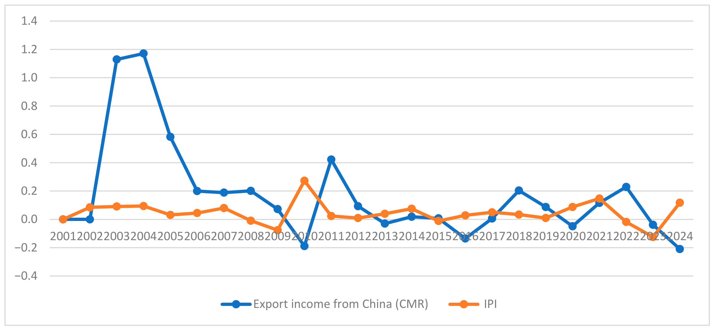
Figure 1 illustrates that Taiwan’s export revenues to China (CMR) and the IPI display notable fluctuations over the 2001–2024 period, with potential lagged and asymmetric co-movements. Several events highlight why a nonlinear framework may be appropriate in this context. Following WTO accession in 2001, cross-strait trade expansion and supply chain integration accelerated [3], yet export performance and industrial production did not always adjust contemporaneously. During the Global Financial Crisis and the COVID-19 pandemic period, export revenues and industrial activity also exhibited uneven timing and adjustment patterns, consistent with delayed industrial responses and regime-dependent dynamics [4,5]. These observations motivate an empirical strategy that can explicitly model regime shifts rather than imposing a constant (linear) relationship between exports and industrial production across the entire sample.

Recent evidence also highlights how trade policy shocks can affect firms through international production networks. Huang et al. [6] examined the 2018–2019 U.S.–China trade war and found that tariff announcements adversely affected firms with greater direct exposure to bilateral trade, with effects also spreading through suppliers and customers in production networks. Their findings illustrate how external trade shocks can influence firms beyond their direct trading relationships. While their study focuses on firm value and trade policy shocks, the present study examines a related but distinct question: does the persistence of Taiwan’s export value growth to Mainland China change with domestic industrial activity?

Although a large body of the literature documents interactions between exports and industrial production—including evidence of bidirectional causality in Taiwan and other economies—most studies rely on linear specifications that assume stable marginal effects across time and states. However, export persistence may depend on the business cycle and may respond differently under low- versus high-activity regimes. This gap is particularly relevant for cross-strait trade, where export patterns are shaped by both structural linkages and episodic shocks.

To address this issue, this study examines whether Taiwan’s export income to China exhibits state-dependent persistence conditional on domestic industrial activity. Using monthly data from June 2001 to October 2024, the analysis models the current-period export value change rate as a function of its lagged value while using the one-period lag of the IPI as a transition variable. Specifically, a Panel Smooth Transition Autoregressive framework is adopted to capture nonlinear adjustments and cross-sectional heterogeneity across export categories, allowing the effect of lagged exports on current exports to vary smoothly across IPI regimes. This study contributes to the literature in three ways: First, it provides evidence on the persistence of Taiwan’s exports to China using a long monthly panel. Second, it identifies whether industrial activity generates a threshold beyond which lagged export performance loses explanatory power. Third, it offers implications for export forecasting and policy design by clarifying when historical export performance is informative and when contemporaneous conditions dominate.

The remainder of this paper is organized as follows: Section 2 reviews the related literature. Section 3 describes the data and methodology, including the linear benchmark and the smooth transition model specification. Section 4 presents the empirical results and robustness checks. Section 5 concludes the study with key findings and implications.

Figure 1. Trends in the rates of change in Taiwan’s export value to Mainland China (CMR) and the Industrial Production Index (IPI), 2001–2024. Source: [1,7].

Figure 1. Trends in the rates of change in Taiwan’s export value to Mainland China (CMR) and the Industrial Production Index (IPI), 2001–2024. Source: [1,7].

2. Literature Review

The Industrial Production Index (IPI) serves as a key indicator of economic health, reflecting the performance of the manufacturing, mining, and utilities sectors. Industrial output not only mirrors domestic economic conditions but also influences a country’s international competitiveness. Trade openness, defined as the extent to which an economy engages in international trade, plays a central role in shaping industrial development. Trade flows are affected by income levels, relative prices, and industrial capacity [8], while export competitiveness is influenced by economies of scale, product differentiation, and market structure [9]. By promoting productivity, fostering technological innovation, and driving structural transformation in domestic industries, greater trade openness often supports higher industrial output, which is reflected in rising IPI values [10].

The relationship between export performance and industrial production has been a central focus in development economics. Early empirical studies suggested that export expansion can stimulate industrial growth by facilitating technology transfer and foreign exchange accumulation. For instance, Riedel et al. [11] reported that India’s export expansion substantially contributed to industrial production growth. Using Sims’ causality framework, Chow [12] examined newly industrialized economies and identified strong bidirectional causality between export performance and industrial output, particularly in Taiwan, Korea, and Singapore. These findings provide support for the export-led industrialization strategies adopted in many Asian economies.

Fung et al. [13] and Leichenko and Coulson [14] showed that export growth and industrial production mutually reinforce one another across countries and regions, highlighting the critical role of industrial production in sustaining export performance. Recent studies have indicated that the relationship between industrial production and exports is neither static nor linear. Using a Panel Smooth Transition Regression (PSTR) framework, Yang et al. [15] showed that Taiwan’s export earnings from China are regime-dependent and that IPI significantly affects export income across different regimes. While the magnitude of the effect varies, these results confirm that higher industrial output generally supports export performance.

Beyond current levels, export patterns display persistence: past export experience and established production capabilities strongly influence present outcomes. Weber et al. [16] linked historical export capacities to sustained competitiveness and income levels, while Dung et al. [17] provided firm-level evidence from Vietnam, showing that exporters rely heavily on previous export experience under changing economic conditions. These findings suggest that export performance is characterized by both persistence and regime-dependent dynamics, implying that conventional linear models may inadequately capture the underlying dynamics of export behavior.

Recent evidence further highlights the importance of examining export persistence in relation to firms’ production capabilities and changing economic conditions. Dung et al. [17] investigated export persistence and productivity in Vietnam, providing additional evidence on the relationship between export activities and productive performance. While their study focused on Vietnam, the present research extends the discussion to Taiwan’s exports to Mainland China by examining whether export value growth persistence varies with domestic industrial activity. In particular, the use of a Panel Smooth Transition Autoregressive (PSTAR) model allows the persistence of export value growth to differ across industrial production regimes.

Recent research has also highlighted the role of global shocks in shaping export fluctuations. Bricongne et al. [18] examined monthly firm-level trade data and found that large exporters played an important role in aggregate export fluctuations, particularly during the global financial crisis and the COVID-19 pandemic. Their findings suggest that export performance may respond heterogeneously to common economic shocks. While their study focused on firm-level export fluctuations in France, the present study investigates whether the persistence of Taiwan’s export value growth to Mainland China varies with domestic industrial activity across 19 export industry groups.

Furthermore, at the firm level, early evidence indicated that diversified production and export structures stabilize sales and increase export persistence by reducing exposure to market-specific shocks, making firms more likely to sustain exporting over time [19]. Building on this dynamic perspective, Love and Máñez [20] showed that export persistence is strongly shaped by learning-by-exporting, whereby accumulated export experience and production routines lower re-entry costs and increase the duration of export spells. At the macro level, export diversification evolves with industrial development along a nonlinear path: expanding industrial production capabilities initially promote the entry and survival of multiple export products, thereby strengthening export persistence, while at higher income levels, re-concentration reflects sustained competitiveness in a narrower set of industries rather than declining export performance [21].

Overall, industrial production is closely linked to export performance, and Taiwan has maintained its competitiveness through strong industrial output despite challenges from cross-strait tensions and global shocks [15,22]. Such dynamic relationships require econometric approaches beyond linear causality. The Panel Smooth Transition Autoregressive (PSTAR) model is particularly suitable in this regard, as it captures nonlinear adjustments and regime-dependent causal effects.

Trade relationships may also exhibit persistence because firms cannot adjust their export destinations and supply chain arrangements instantaneously. Benguria and Saffie [23] examined the effects of the U.S.–China trade war and showed that financial constraints and the persistence of trading relationships influenced how exporters redirected their sales toward alternative markets. Their findings highlight the importance of considering both external trade shocks and the durability of established trade relationships when analyzing export dynamics. Building on this perspective, the present study examines whether the persistence of Taiwan’s export value growth to Mainland China varies with domestic industrial activity.

Linear models often fail to represent complex macroeconomic dynamics [24,25,26]. Hansen’s Panel Threshold Regression (PTR) allows regime shifts but may inadequately identify regimes in complex data. González et al. [24] developed the Panel Smooth Transition Regression (PSTR) to allow smooth coefficient variation, though it is limited by degrees of freedom and low-frequency data. PSTAR extends PSTR by incorporating autoregressive dynamics and lagged dependent variables, capturing delayed adjustments and sharp behavioral changes.

Findings from PSTR and PSTAR estimations [10,27] indicate that FDI and trade openness influence economic growth in a nonlinear, threshold-dependent manner. By capturing these regime-specific dynamics, PSTAR offers a flexible and robust framework for analyzing complex macroeconomic relationships. Recent developments in nonlinear time series analysis have extended threshold autoregressive models to accommodate more complex regime-dependent dynamics. Zhang et al. [28] proposed a two-threshold-variable integer-valued autoregressive model and examined its statistical properties and estimation performance. Although their model differs from the continuous-valued panel framework adopted in this study, their work illustrates the continuing development of threshold-based autoregressive methods for capturing nonlinear dynamic behavior.

Economic and financial time series may exhibit complex dependence structures that cannot always be adequately represented by conventional linear models. Giannerini and Goracci [29] discussed entropy-based tests for complex dependence in economic and financial time series, highlighting the importance of appropriate diagnostic tools when investigating nonlinear dynamics. This perspective supports the use of formal nonlinearity testing before estimating a nonlinear autoregressive specification. Building on this approach, Section 3 employs the PSTAR model to investigate Taiwan’s trade with China, demonstrating its advantages over conventional linear methods.

3. Data and Methodology

3.1. Research Data

This study uses monthly panel data covering the period from June 2001 to October 2024, comprising 19 export industry groups, as listed in Table 1. The sample covers 281 months, resulting in a balanced panel with no missing observations. Accordingly, the dataset contains 5339 observations (N × T = 19 × 281), where N = 19 represents the number of industry groups and T = 281 represents the number of monthly periods.

Table 1. Industry classification and cross-sectional units.

No.	Industry Group	No.	Industry Group	No.	Industry Group
1	Live Animals; Animal Products	8	Fur and Articles Thereof	15	Base Metals and Articles of Metal
2	Vegetable Products	9	Wood and Articles of Wood	16	Machinery and Electrical
3	Animal or Vegetable Fats and Oils	10	Pulp, Paper, and Printing Products	17	Aircraft, Vehicles, Vessels, and Associated Transport Equipment
4	Prepared Foodstuffs; Beverages, Spirits, and Tobacco Products	11	Textiles and Textile Articles	18	Optical, Precision Instruments; Clocks and Watches; Musical Instruments
5	Mineral Products	12	Footwear, Headgear, Umbrellas; Artificial Flowers; Articles of Human Hair	19	Others
6	Chemicals	13	Articles of Stone, Plaster, and Cement; Ceramic Products; Glass and Glassware
7	Plastics and Articles Thereof; Rubber and Articles Thereof	14	Precious Stones, Pearls, and Precious Metals; Coin; Imitation Jewelry

Table 2 presents the variables and their symbols, measurements, and data sources. The dependent variable, CMR, represents the rate of change in Taiwan’s export value to Mainland China. The explanatory variable, CMRL1, is the one-period lag of CMR. The transition variable, IPIL1, is the one-period lag of Taiwan’s Industrial Production Index.

Table 2. Data measurement.

Variable	Symbol	Measurement	Sources
Rate of change in Taiwan’s export value to Mainland China	CMRit	The proportion of change in the export values over the current period (t) minus the prior period (t − 1), divided by the previous period (t − 1), and multiplied by 100%	Ministry of Finance, R.O.C.
Taiwan’s IPI change rate (lagged by one period)	IPIL1t−1	The proportion of fluctuation in IPI of Taiwan over a lag of 1 period (t − 1) minus the prior period (t − 2) and divided with the prior period (t − 2), then multiplied by 100%	National Statistics, R.O.C.
One-period lagged rate of change in Taiwan’s export value to Mainland China	CMRL1i,t−1	The percentage of variation in the export value over a lag of 1 period (t − 1) minus the prior period (t − 2) and divided with the prior period (t − 2), then multiplied by 100%	Ministry of Finance, R.O.C.

3.2. Linear Model

Following the methodological recommendations of Yang et al. [30], the analysis examines the threshold impacts of the IPI on the persistence of Taiwan’s export value change rate to Mainland China (June 2001 to October 2024). The empirical linear model is expressed as shown in Equation (1):

CMR_it = α₀ + α₁CMRL1_i,t−1 + ε_it

(1)

For each i = 1, 2, …, N and t = 1, 2, …, T, N and T denote the number of cross-sectional industries and the number of time periods in the panel, respectively; CMR_it represents Taiwan’s export income of industry (i) in the current period (t); CMRL1_it−1 represents Taiwan’s export earnings of industry (i) in the period (t − 1); and ε_it is a residual term.

Additionally, autoregressive models can be interpreted as a form of regression model which is applied to lagged series generated from the original time series. In light of the cyclical trends observed in the export data, this study adopted a lag length of four periods. To identify which lagged export value change rate variables significantly influence the current period of export performance, the first, second, third, and fourth lags of the rate of change in Taiwan’s export value to Mainland China are statistically tested. Based on this specification, the autoregressive model of firm performance can be written as Equation (2):

CMR_it = α₀ + α₁CMRL1_i,t−1 + α₂CMRL2_i,t−2 + α₃CMRL3_i,t−3 + α₄CMRL4_i,t−4 + ε_it

(2)

where i = 1, 2, …, N and t = 1, 2, …, T, with N denoting the number of cross-sectional industries and T representing the number of time periods in the panel. CMR_it represents Taiwan’s export income of industry (i) in the current period (t), and CMRL1_i,t−1, CMRL2_i,t−2, CMRL3_i,t−3, and CMRL4_i,t−4 indicate Taiwan’s export income of the same industry (i) in the first, second, third, and fourth lagged periods, respectively; and ε_it is a residual term.

3.3. PSTAR Model

To simultaneously address the issues of nonlinearity and heterogeneity, this study applies the PSTAR model developed by González et al. [24], as shown in Equation (3):

CMR_it = α_i + α₀CMRL1_i,t−1 + α₁CMRL1_i,t−1G(q_it; γ; c) + ε_it

(3)

where i = 1, 2, …, N and t = 1, 2, …, T, with N representing the number of cross-sectional industries and T denoting time. CMR_it represents the rate of change in Taiwan’s export value for export of industry (i) of the current period (t), and CMRL1_i,t−1 denotes Taiwan’s export value change rate of industry (i) in the period (t − 1). In the model, α₀ denotes the individual fixed effect, capturing time-invariant heterogeneity across observational units. The transition function is G(q_it; γ; c), with values ranging from 0 to 1, characterizing the smooth shift between difference regimes. With q_it as a transition variable, the parameter γ specifies the transition speed, reflecting the intensity or smoothness of the nonlinear adjustment process, while c indicates the transition threshold, and the residual term is represented by ε_it. Furthermore, both the lagged transition variable and the optimal value for the current period need to be determined using the Bayesian Information Criterion (BIC) and the Akaike Information Criterion (AIC) to find the minimum value. Therefore, this study replaces q_it with q_it−d, d = 0, 1, …, 4 based on the logistic specification of González et al. [24] for the transition function, as specified in Equation (4):

$$G(q_{\mathit{it}};\gamma ;c)={(1+\mathit{exp}(-\gamma {\mathsf{\Pi }}_{j=1}^m(q_{\mathit{it}}-c_j)\left)\right)}^{-1}$$

(4)

where γ > 0 and c₁ ≤ c₂≤ ⋯ ≤c_m, with c = (c, c,…,c) representing an m dimensional vector of location parameters, and the slope parameter γ determines transitions’ smoothness, which means that the larger the γ value, the steeper (.) the slope of G. When m = 1 and γ → ∞, the PSTAR model declines to a panel transition regression model. According to González et al. [24], the value of m = 1 or m = 2 is sufficient. When m is 1, the transition function divides the data into two distinct regimes, which are based on the threshold value. Conversely, when m has a value of two, the threshold value divides the data into three regimes. The general specification of the PSTAR model is presented in Equation (5):

$${\mathit{CMR}}_{\mathit{it}}={\alpha }_i+{\alpha }_0{CMRL1}_{i,t-1}+{\sum }_{j=1}^r{\alpha }_j{CMRL1}_{i,t-1}{G}_j(q_{\mathit{it}};\gamma ;c)+{\epsilon }_{\mathit{it}}$$

(5)

where the transition quantity in the model is denoted by j = 1, 2,…, r and (r + 1) indicates the total number of regimes.

3.4. Linearity and Remaining Nonlinearity Tests

As part of the research methodology, linearity and the unavailability of remaining nonlinearity were tested to make sure the model is correctly specified. To this end, the following auxiliary equation was estimated as Equation (6):

CMR_it = α_i + α₁CMRL1_i,t−1 + α′₁CMRL1_i,t−1q_t−d + ε_it

(6)

where d = 0, 1,…, 5, corresponding to current and lagged export value change rate terms. The linearity examination is implemented to evaluate the null hypothesis, H₀: α′₁ = 0. Rejection of the null hypothesis implies the presence of nonlinearity, prompting further testing of a single-threshold specification against a double-threshold alternative. This sequential examining process will not stop until the null hypothesis of no additional threshold cannot be rejected. In this framework, PSSR₀ represents the total sum of squared residuals under the null hypothesis, which corresponds to the linear panel model with individual effects, while (PSSR₁) is defined as the total sum of squared residuals under the alternative, specifically the PSTAR model with two separate regimes. The associated LM statistic is then computed according to Equation (7):

LM_F = [(PSSR₀ − PSSR₁)/K]/[PSSR₀/(TN − N − K)]

(7)

where K denotes the number of explanatory variables. The LM statistic exhibits an asymptotic X²(K) distribution under the null hypothesis.

4. Findings

4.1. Descriptive Statistics

Table 3 illustrates the study’s IPI and export revenue descriptive data. Each variable’s maximum, minimum, mean, and standard deviation are included in the table to show their distributional properties and temporal fluctuations during the observation period.

Table 3. Descriptive statistics.

	CMR	IPIL1	CMRL1
Mean	0.090081	0.007242	0.090911
Maximum	20.62295	0.315245	20.62295
Minimum	−0.931726	−0.214089	−1.000000
Std. Dev	0.706778	0.085427	0.708482
Observations	5339	5339	5339

Note: (1) CMR_it is the current-period export value change rate, CMRL1_it−1 denotes the export value change rate lagged by 1 period, and IPIL1_t−1 is the IPI lagged by 1 period. (2) The sample period is from June 2001 to October 2024.

Table 2 demonstrates that among all the observed variables, CMR exhibits the widest range of values, extending from a maximum of 20.62295 to a minimum of −0.931726. Both CMR and its first lag (CMRL1) show relatively high standard deviations of approximately 0.71, in contrast to IPIL1, which records a much lower standard deviation of 0.085. This notable difference suggests that Taiwan’s IPI tends to remain relatively stable over time, whereas export-related variables experience greater fluctuations. The low variation in IPIL1 may also reflect that Taiwan’s IPI has been less sensitive to short-term shocks, despite the extreme change observed in export performance.

Furthermore, there is a large gap between the maximum and minimum values of CMR and CMRL1, with the highest peak reaching 20.62 and the lowest point approaching −1.00, indicating that Taiwan’s exports have undergone both significant periods of expansion and contraction, corresponding to phases of economic growth and recession. The reduced mean (0.0072) and standard deviation (0.0854) of IPIL1 show a steady but modest upward trend in Taiwan’s industrial production. While exports are more volatile and prone to external shocks, the country’s industrial production sector has maintained a gradual and sustained growth trajectory during the observed period.

4.2. Hausman Test

By including the Hausman test into its framework, the PSTAR model may ascertain whether using random effects or fixed effects in the model specification is superior. The alternative hypothesis H₁ and null hypothesis H₀ are as follows:

H₀. 

The random effect.

H₁. 

The fixed effect.

When the p-value of the test is statistically significant, which illustrates that the null hypothesis (H₀) needs to be rejected, the fixed effects model becomes the superior option. If the p-value is not significant, however, the random effects model is a better fit. As shown in Table 4, the p-value (Prob.) is 0.00000, which is less than the 0.01 significance level (the level of statistical significance). This finding is so statistically significant that it allows us to reject the null hypothesis (H₀) and embrace the alternative hypothesis (H₁). Consequently, the fixed effects model was the most effective in estimating the linear panel data model.

Table 4. Hausman test.

Test Summary	Chi-Sq. Statistic	Chi-Sq. d.f.	p-Value
Cross-section	86.081865	1	0.0000 ***

Note: *** indicate significance at 1% level.

4.3. Nonlinear Panel Unit Root Test

The Augmented Dickey–Fuller (ADF) test was used to determine whether each variable was stationary, guaranteeing that non-stationary data would not influence empirical calculations. In particular, the test was implemented to assess the presence of a nonlinear effect. The null hypothesis H₀ and alternative hypothesis H₁ of the nonlinear panel unit root test are shown below:

H₀. 

The variable has a unit root.

H₁. 

The variable does not have a unit root.

If the p-value of a given variable was found to be statistically significant, it indicated rejection of the null hypothesis (H₀) and acceptance of the alternative hypothesis (H₁), suggesting that the series was stationary. The detailed results of the ADF test for all variables are shown in Table 5 below.

Table 5. Nonlinear panel unit root test results.

Variables	Augmented Dickey– Fuller Test Statistic	Break Date	Lag
CMRit	−13.58505 ***	Sep. 2023 (0550M09)	11
IPIL1t−1	−16.14872 ***	Aug. 2023 (0549M08)	11
CMRL1it−1	−13.43431 ***	Oct. 2023 (0550M10)	11

Note: (1) *** indicate significance at 1% level; (2) same as Table 3, Note 1.

The results in Table 5 show that all variables are strongly significant, indicating that the null hypothesis (H₀) can be rejected and the alternative hypothesis “without unit root” was accepted. Both the time series and cross-sectional components of the panel data demonstrate stability, confirming that the dataset is stationary and suitable for further econometric study. These findings enabled the implementation of the nonlinearity test in this study.

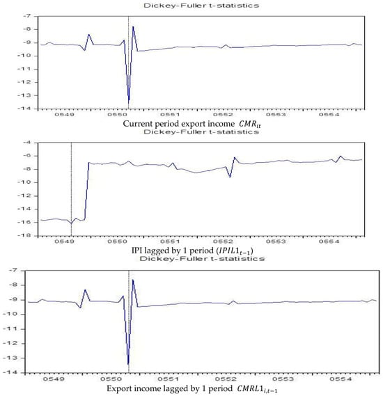
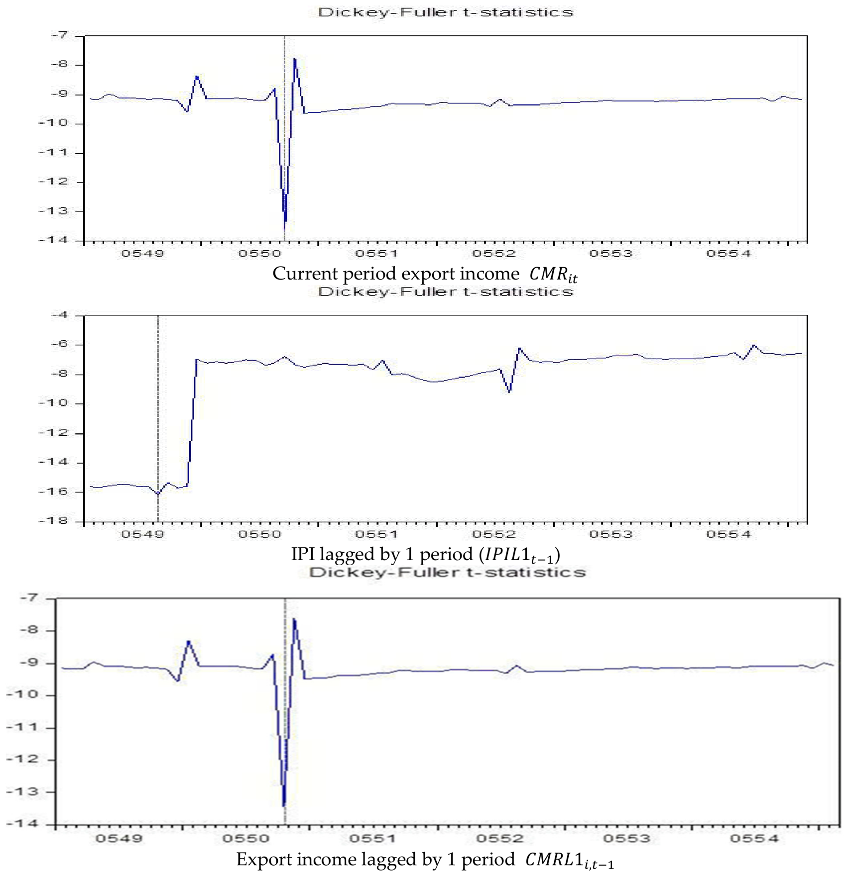
The unit root test results for the current-period export value change rate (CMR_it), one-period lagged export value change rate (CMRL1_it−1), and the IPI lagged by one period (IPIL1_t−1) from June 2001 to October 2024 are shown in Figure 2. The turning point, shown by the dotted lines in the figure, occurred in September 2023 (0550M09), August 2023 (0549M08), and October 2023 (0550M10). As shown in Table 5 and Figure 2, all variables are statistically significant, suggesting that the series exhibits nonlinear structural transformation and is expected to converge toward stability over time. These findings suggest regime shifts and unequal adaptations, supporting the adoption of a nonlinear framework like the PSTAR model to capture the dynamic connection between Taiwan’s export income and the IPI.

Figure 2. Dickey–Fuller autoregressive coefficient test of CMR_it, IPIL1_t−1, and CMRL1_i,t−1. Note: Same as in Table 3, Note 2.

4.4. Autoregression Test

In order to ascertain statistical significance, the auto-regression testing formula (2) was employed to evaluate four potential variables: CMRL1, CMRL2, CMRL3, and CMRL4. The statistical significance of CMRL1, CMRL2, and CMRL3 is demonstrated in Table 6, suggesting that these lagged variables could initially be considered for incorporation into the PSTAR model. However, when the candidate lagged variables were incorporated into the PSTAR specification, CMRL2 and CMRL3 became statistically insignificant, whereas CMRL1 remained statistically significant. Therefore, CMRL1 was selected as the independent variable in the final PSTAR model.

Table 6. Autoregression test.

Variable	Coefficient	Std. Error	t-Statistic	Prob.
CMRL1	−0.121756	0.013615	−8.943040	0.0000 ***
CMRL2	0.094260	0.013642	6.909680	0.0000 ***
CMRL3	0.051810	0.009578	5.409195	0.0000 ***
CMRL4	0.007905	0.009540	0.828654	0.4073
R-squared	0.014027	Mean dependent	VAR	0.090081

Note: *** indicate significance at 1% level.

4.5. Linearity Test

The nonlinear panel unit root test result confirmed the stationarity of all variables. Thus, it was appropriate to proceed with examining the potential nonlinear relationship between Taiwan’s export income from China and its IPI. The null and alternative hypotheses are stated below:

H₀. 

The PSTAR model was linear.

H₁. 

The PSTAR model (nonlinear) had at least one threshold variable (r = 1).

If the r value for each variable was found to be significant, this indicated that the null hypothesis H₀ was rejected, while the alternative hypothesis H₁ was accepted. The results of the linearity test are presented in Table 7.

Table 7. Linearity test results.

Test Statistic	Number of Location	Number of Location
	Parameters (m)	Parameters (m)
	m = 1	m = 2
Wald Test (LM)	23.648 (0.000) ***	23.932 (0.000) ***
Fisher Test (LMF)	23.665 (0.000) ***	11.973 (0.000) ***
LRT (LRT)	23.701 (0.000) ***	23.986 (0.000) ***

Note: (1) H₀: Linear model. H₁: PSTAR model with at least one threshold variable (r = 1). (2) *** indicate significance at 1% level.

Table 7 shows the results of the Wald test, Fisher test, and LRT conducted to examine the linearity of the connection between export income and the IPI. The significance level of this result rejects the null hypothesis of linearity at the location parameters of one (m = 1) and two (m = 2). This rejection implies that the underlying relationship between export earnings and the IPI is not adequately captured by a simple linear model. Instead, the findings suggest that there are certain points or ranges in the IPI where the relationship with export income changes abruptly, indicating the presence of structural changes or threshold effects that influence export income differently at various IPI levels.

Given these conclusions, it is both essential and suitable to use a nonlinear specification to appropriately characterize the dynamics among the variables. Reduced AIC and BIC values signify a more parsimonious and superior model fit, hence ensuring the robustness of the estimate outcomes. The subsequent section provides a detailed explanation of the procedure used to identify the optimal number of threshold regimes and the corresponding threshold values within the nonlinear framework.

4.6. The Optimal Number of Threshold Regimes

Given the presence of a nonlinear relationship between export income and the IPI, the optimal number of threshold regimes was further examined in this research. The corresponding null and alternative hypotheses are specified as follows:

H₀. 

PSTAR with r = 1

H₁. 

PSTAR with at least r = 2

For the remaining nonlinearity test, a statistically significant result indicates rejection of the null hypothesis (H₀) in favor of the alternative hypothesis (H₁), whereas a non-significant result indicates a failure to reject H₀. The results of the remaining nonlinearity tests are shown in Table 8.

Table 8. Results of remaining nonlinearity tests.

Test Statistic	Number of Location	Number of Location
	Parameters (m)	Parameters (m)
	m = 1	m = 2
Wald Test (LM)	0.027 (0.869)	0.000 (1.000)
Fisher Test (LMF)	0.027 (0.869)	0.000 (1.000)
LRT (LRT)	0.027 (0.869)	0.000 (1.000)

The remaining nonlinearity test was conducted under two different model specifications: one with a single location parameter (m = 1) and another with two location parameters (m = 2). The corresponding results for both cases are illustrated in Table 8; the Wald test, Fisher test, and LRT test are not statistically significant at conventional significance levels.

Since the null hypothesis states that there is no additional nonlinearity, while the alternative hypothesis indicates the presence of additional nonlinearity, the absence of statistical significance indicates a failure to reject the null hypothesis. The results for both specifications (m = 1 and m = 2) suggest that there is insufficient statistical evidence to support the inclusion of an additional transition function. Therefore, the model with one transition function is selected as the preferred specification.

4.7. Empirical Results of PSTAR Model

After completing the earlier tests, the PSTAR model was applied to assess the impact of the IPI on export income. Overall, this research contributes significantly to the existing literature on this subject. First, the PSTAR model measured the persistence of export income, enabling the analysis of nonlinear dynamics and cross-sectional heterogeneity in export performance. Second, the study incorporated a transition variable into the model, capturing shifts and persistence patterns in export income. Furthermore, by using the AIC and BIC to identify the optimal model, a PSTAR model for analyzing the persistence of export income was established, as shown in Table 9.

Table 9. Results of PSTAR model.

Model Parameter	PSTAR Model	Linear Panel Data Model
∁	−	0.1035 (0.0096) ***
α1	4.4925 (1.3859) ***	−0.1474 (0.0135) ***
α1′	−4.4925 (1.3649) ***	−
r	2.6976	−
c	0.04920	−
N	5339	5339
AIC	0.7345	−
BIC	0.7296	−
R-squared	−	0.021842
Hausman test	−	0.0000 ***

Note: α₁ and α₁′ are the one-period lagged rate of change in Taiwan’s export value to Mainland China. α₁ + ${\alpha }_1^{\prime }$ = 0. The values in brackets are the t-statistics. *** indicate significance at 1% level.

In the linear model, the estimated coefficient of the independent variable (CMRL1) is −0.1474 with a standard error of 0.0135, which is statistically significant at the 1% level (***). This result illustrates a negative relationship between export income in the previous period and current-period export value growth rate. Specifically, holding other factors constant, a one-unit increase in Taiwan’s export income lagged by one period leads, on average, to a 0.1474-unit decrease in the current period’s export income. This finding indicates a short-term adjustment or correction effect in Taiwan’s export dynamics.

In the PSTAR model, the estimated threshold value c and transition parameter γ are 0.04920 and 2.6976, respectively. The estimated coefficients of 4.4925 and −4.4925 describe the limiting regimes of the smooth transition model. The effective coefficient of CMRL1 depends on the value of the transition function and varies smoothly with the transition variable IPIL1, rather than changing abruptly at the threshold. These results indicate that the persistence of Taiwan’s export value change rate varies with changes in the industrial production index through a smooth transition process.

5. Conclusions

To assess the relationship between Taiwan’s industrial activity and export income, we used a PSTAR model to examine the overall data. The export value change rate lagged by one period (CMRL1) was used as the independent variable and the current-period export value change rate (CMR) as the dependent variable. The transition variable was Taiwan’s IPI lagged by one period (IPIL1). Based on an empirical study, the IPI of Taiwan significantly influences the effect of CMRL1 on CMR.

When IPIL1 is below the threshold value of 0.04920, the estimated low-regime coefficient for CMRL1 is 4.4925, indicating a positive and statistically significant relationship between the lagged and current export value change rates. This finding suggests that, under the low-IPIL1 regime, the current-period export value change rate is positively associated with its one-period lagged value, reflecting persistence in export performance. This finding indicates that, under the low-IPIL1 regime, the current-period export value change rate is positively associated with its one-period lagged value, reflecting persistence in export performance. Revenue from exports that is more than a year old makes up a significant chunk of the total since industrial activity and export demand are both low when the IPI is below the threshold. Companies frequently depend on factors like accumulated production capacity, historical contracts, and existing trade relationships. The economy’s dependence on delayed export income can be improved by increasing output and reviving export momentum via stimulating industrial activity.

When IPIL1 is greater than 0.04920, a one-unit increase in CMRL1 has little effect on CMR. Although the constant term and the lagged export value change rate term are both fairly large, they cancel each other out, resulting in a net effect close to zero. Lagged and current export revenue have a weaker association when the IPI exceeds the threshold, according to economic arguments. On the contrary, it is propelled by more generic international factors, production capacity, market demand, and export competitiveness. Although IPIL1 and CMRL1 both increase, their combined effect on CMR is insignificant. There has thus been a regime shift in the criteria used to calculate export income, with an emphasis on real-time conditions instead of historical patterns.

The effect of the lagged export value change rate on the current-period export value change rate decreases significantly when the IPI rises from below the threshold to above it. The low-IPI regime places significant emphasis on accumulated production capacity and established trade relationships when planning future exports. At the threshold of the IPI, current economic conditions (i.e., production levels, market demand, and competitiveness) take over as the primary determinants of export revenue, rendering postponed export revenue largely irrelevant. Companies are now more agile and adapt their strategies on the fly, reflecting a shift away from relying on historical trends and toward responding to current events.

A vital lesson for companies may be gleaned from these findings; namely, it is essential to identify when present conditions take center stage and when the lagged export value change rate drives the current-period export value growth rate. Income from exports is highly dependent on pre-existing relationships and prior knowledge when industrial activity is below the cutoff. Nevertheless, when industrial activity surpasses a certain threshold, a clear regime shift occurs. At this point, market circumstances surpass prior patterns, necessitating immediate responses and plan adjustments from firms.

Further research on the interplay between this regime shift and external forces including currency rate fluctuations, changes in global demand, and interruptions to the supply chain could shed light on the export dynamics at play. More research into industry-specific thresholds or cross-country comparisons can also provide insights into whether this structural transition is peculiar to Taiwan or reflects a more widespread trend in export-driven economies.

References

- Department of Statistics, Ministry of Finance. Annual External Trade Report in 2024. 2025. Available online: https://service.mof.gov.tw/public/Data/statistic/bulletin/114/113%E5%B9%B4%E6%88%91%E5%9C%8B%E5%87%BA%E9%80%B2%E5%8F%A3%E8%B2%BF%E6%98%93%E6%A6%82%E6%B3%81_%E8%8B%B1%E6%96%87%E7%89%88_%E4%B8%8A%E7%B6%B2.pdf?utm_source=chatgpt.com (accessed on 25 February 2025).
- Feng, K.W.; Huang, C.H. The Impact of Exchange Rate Fluctuations on Taiwan-U.S. Trade: An Analysis Using Industry Level Trade Data. Master’s Thesis, National Tsing Hua University, Hsinchu, Taiwan, 2020. [Google Scholar]
- Hsu, K. Taiwan’s role in the global supply chain: Trends of decentralization and relocation, challenges, and prospects. Taiwan Strateg. 2023, 19, 37–55. [Google Scholar]
- Himpler, J.P. The world financial crisis: Impacts on GDP and international trade in Taiwan. In Crisis Management: Theory and Practice; IntechOpen: London, UK, 2018; p. 115. [Google Scholar] [CrossRef] [Scilit]
- Tsai, I.J. Trade options for a small open economy: The different impact of Taiwan exports to China and to other countries. J. Policy Model. 2023, 45, 202–227. [Google Scholar] [CrossRef] [Scilit]
- Huang, Y.; Lin, C.; Liu, S.; Tang, H. Trade networks and firm value: Evidence from the U.S.-China trade war. J. Int. Econ. 2023, 145, 103811. [Google Scholar] [CrossRef] [Scilit]
- National Statistics, Republic of China (Taiwan). 2025. Available online: https://www.moea.gov.tw/Mns/dos_e/bulletin/Bulletin_En.aspx?kind=13&html=1&menu_id=6743&bull_id=16574 (accessed on 25 February 2025).
- Houthakker, H.S.; Magee, S.P. Income and price elasticities in world trade. Rev. Econ. Stat. 1969, 51, 111. [Google Scholar] [CrossRef] [Scilit]
- Krugman, P. Scale economies, product differentiation, and the pattern of trade. Am. Econ. Rev. 1980, 70, 950–959. [Google Scholar]
- Trabelsi, R.; Kalai, M.; Helali, K. The nonlinear impact of trade openness on the economic growth in Maghreb countries. Qual. Quant. 2025, 60, 1081–1102. [Google Scholar] [CrossRef] [Scilit]
- Riedel, J.; Hall, C.; Grawe, R. Determinants of Indian export performance in the 1970s. Weltwirtschaftliches Arch. 1984, 120, 40–63. [Google Scholar] [CrossRef] [Scilit]
- Chow, P.C. Causality between export growth and industrial development: Empirical evidence from the NICs. J. Dev. Econ. 1987, 26, 55–63. [Google Scholar] [CrossRef] [Scilit]
- Fung, H.G.; Sawhney, B.; Lo, W.C.; Xiang, P. Exports, imports and industrial production: Evidence from advanced and newly industrializing countries. Int. Econ. J. 1994, 8, 87–98. [Google Scholar] [CrossRef]
- Leichenko, R.M.; Coulson, N.E. Foreign industrial exports and state manufacturing performance. Growth Change 1999, 30, 479–506. [Google Scholar] [CrossRef] [Scilit]
- Yang, T.Y.; Liu, C.; Yang, Y.T.; Chen, S.H. The dynamic effect of trading between China and Taiwan under exchange rate fluctuations. Humanit. Soc. Sci. Commun. 2023, 10, 1–9. [Google Scholar] [CrossRef] [Scilit]
- Weber, I.; Semieniuk, G.; Liang, J.; Westland, T. Persistence in World Export Patterns and Productive Capabilities Across Two; Working Paper No. 2022-11; University of Massachusetts Amherst: Amherst, MA, USA, 2022. [Google Scholar]
- Dung, D.T.K.; Van Bao, N.; Thuong, P.T.S.; Thuy, H.T.K. Export persistence and productivity in Vietnam. J. Econ. Integr. 2024, 39, 714–749. [Google Scholar] [CrossRef] [Scilit]
- Bricongne, J.-C.; Carluccio, J.; Fontagné, L.; Gaulier, G.; Stumpner, S. From macro to micro: Large exporters coping with global crises. J. Int. Econ. 2025, 153, 104037. [Google Scholar] [CrossRef] [Scilit]
- Hirsch, S.; Lev, B. Sales stabilization through export diversification. Rev. Econ. Stat. 1971, 53, 270–277. [Google Scholar] [CrossRef] [Scilit]
- Love, J.H.; Máñez, J.A. Persistence in exporting: Cumulative and punctuated learning effects. Int. Bus. Rev. 2019, 28, 74–89. [Google Scholar] [CrossRef] [Scilit]
- Cadot, O.; Carrère, C.; Strauss-Kahn, V. Export diversification: What’s behind the hump? Rev. Econ. Stat. 2011, 93, 590–605. [Google Scholar] [CrossRef] [Scilit]
- Tsai, F.W.; Bernard, P., Jr.; Plaisent, M.; Lin, E.Y. A regression analysis on the macroeconomic variables affecting Taiwan’s export value to the US before and after 2008 financial crisis. J. Comp. Int. Manag. 2014, 17, 43–65. [Google Scholar]
- Benguria, F.; Saffie, F. Escaping the trade war: Finance and relational supply chains in the adjustment to trade policy shocks. J. Int. Econ. 2024, 152, 103987. [Google Scholar] [CrossRef] [Scilit]
- González, A.; Teräsvirta, T.; van Dijk, D.; Yang, Y. Panel Smooth Transition Regression Models; EFI Working Paper No. 604; Stockholm School of Economics: Stockholm, Sweden, 2005. [Google Scholar]
- Hansen, B.E. Threshold effects in non-dynamic panels: Estimation, testing, and inference. J. Econom. 1999, 93, 345–368. [Google Scholar] [CrossRef] [Scilit]
- Teräsvirta, T. Specification, estimation, and evaluation of smooth transition autoregressive models. J. Am. Stat. Assoc. 1994, 89, 208–218. [Google Scholar] [CrossRef] [Scilit] [PubMed]
- Helali, K.; Kalai, M. Threshold effect of foreign direct investment on economic growth: New evidence from a panel regime switching models. Res. Sq. 2021. [Google Scholar] [CrossRef] [Scilit] [PubMed]
- Zhang, J.; Zhu, F.; Chen, H. Two-Threshold-Variable Integer-Valued Autoregressive Model. Mathematics 2023, 11, 3586. [Google Scholar] [CrossRef] [Scilit]
- Giannerini, S.; Goracci, G. Entropy-Based Tests for Complex Dependence in Economic and Financial Time Series with the R Package tseriesEntropy. Mathematics 2023, 11, 757. [Google Scholar] [CrossRef] [Scilit]
- Yang, T.Y.; Yang, Y.T.; Chen, S.H.; Lan, Y.T.; Peng, C.J. Dynamic effect of economic growth on the persistence of suicide rates. Geospat. Health 2023, 18, 1201. [Google Scholar] [CrossRef] [Scilit] [PubMed]
Disclaimer/Publisher’s Note: The statements, opinions and data contained in all publications are solely those of the individual author(s) and contributor(s) and not of MDPI and/or the editor(s). MDPI and/or the editor(s) disclaim responsibility for any injury to people or property resulting from any ideas, methods, instructions or products referred to in the content. |
© 2026 by the authors. Licensee MDPI, Basel, Switzerland. This article is an open access article distributed under the terms and conditions of the Creative Commons Attribution (CC BY) license.