


Abstract
Recommendation systems change both the amount and allocation of exposure opportunities, making their effects on diffusion difficult to separate. We develop a discrete-time unexposed–exposed–active–inactive (UEAI) model that links static stance consistency, target-specific recommendation visibility and active-prevalence feedback. For this model, we derive sparse dynamic message-passing (DMP) equations. Exact per-time-step matching of degree-weighted potential edge-opportunity budgets isolates allocation changes. We prove that equal budgets can produce different expected new adoptions. Paired Monte Carlo (MC) simulations on Barabási–Albert and stochastic block model networks show a positive median network-level advantage in final cumulative adoption under dynamic recommendation over uniform budget-matched allocation. Constructive counterexamples establish that a shared local non-backtracking stability boundary need not determine finite-network stochastic early-growth boundaries or macroscopic cascade transitions. Across four synthetic network families, numerical boundary estimates vary with topology, seed and observation criteria. DMP approximates final adoption and active-fraction trajectories. In some parameter tests, however, its predicted change in the dynamic-minus-matched adoption advantage has the opposite sign to the MC result. The framework supports comparisons of recommendation allocation at equal potential budgets and requires propagation boundaries to be interpreted according to their distinct physical criteria.
Keywords:
information diffusion; recommender systems; dynamic message passing; recommendation-opportunity allocation; propagation boundaries; network topology MSC:
91D30; 05C82
1. Introduction
1.1. Recommendation-Mediated Diffusion of Stance-Bearing Information
Recommendation systems mitigate information overload by selecting and personalizing content [1]. In online social networks, ranking can alter relative exposure to political content [2], contribute to misinformation recommendation and diffusion [3], and alter encountered content and platform use without detectable changes in the measured political attitudes over a three-month study [4]. Through this allocation of visibility, recommendation links network structure to exposure opportunities.
Feedback from clicks, interactions and popularity can change opportunity allocation as diffusion unfolds. Joint recommendation–diffusion models incorporate user relationships, opinion similarity, and temporal information [5]. Related studies identify algorithmic confounding and homogenization [6], persistent exposure inequality [7], feedback loops and bias amplification [8], and reciprocal user–recommender feedback [9]. Social relations can inform preference modeling, but low preference-aware homophily limits their value as a proxy for preferences [10]. Recommendation therefore affects both the total opportunity budget and its allocation across target nodes.
For stance-bearing information, prior research has examined ideological exposure and selective consumption [11], homogeneous misinformation-sharing communities [12], distinct diffusion patterns for true and false news [13], homophilous interaction and diffusion across platforms [14], and user interaction in YouTube vaccine-related echo chambers [15]. User and information stances remain fixed within each diffusion realization, allowing recommendation allocation to be studied separately from opinion evolution. User–information stance consistency enters recommendation visibility and post-exposure adoption through separate rules. State transitions then track exposure, adoption, and cessation of transmission.
1.2. Research Gaps in Recommendation-Mediated Diffusion
Reviews synthesize diffusion models and evaluation methods [16,17]. Activation and rumor models describe propagation processes [18,19], while network models and degree correlations provide structural foundations [20,21,22,23,24]. Core–periphery organization can also affect reach and critical behavior [25]. Extensions address cross-network and temporal effects [26,27], node-level heterogeneity [28,29,30,31], and multilayer or higher-order interactions [32,33,34,35,36].
Recommendation–diffusion studies examine social-content and misinformation recommendation and online information diffusion [3,5,37], algorithmic personalization in opinion dynamics [38], feed ranking effects on misinformation and polarization [39], learning-based recommenders coupled to opinion updating [40], and affinity-driven recommendation coupled to misinformation diffusion [41]. We ask whether different allocations yield equivalent diffusion outcomes when their degree-weighted potential edge-opportunity budgets are matched at each time step. This budget is the in-degree-weighted sum of target-specific visibility.
Dynamic message passing (DMP) approximates diffusion through directed-edge cavity messages under tree-like or locally tree-like conditions [42,43]. Non-backtracking linearization links local stability to spectral structure [44]. We assess finite-network DMP accuracy against Monte Carlo (MC) simulations because short cycles, clustering and overlapping paths violate cavity independence. Clustering can also affect thresholds and conditional final sizes [45], coupling and topological representation affect critical behavior [32,33,34,35], and relative timescales affect epidemic–opinion peak magnitude and timing [36]. These findings motivate distinguishing local instability of infinitesimal perturbations, finite-window stochastic early growth retaining extinction, and macroscopic cascades defined by coverage and occurrence probability. Whether the local boundary represents the latter criteria is separate from DMP’s dynamical accuracy.
1.3. Research Questions and Main Contributions
We develop a discrete-time unexposed–exposed–active–inactive (UEAI) model coupling network contact, target-specific recommendation visibility, static stance consistency, and active-prevalence feedback. We address three research questions: RQ1 evaluates the DMP approximation, whereas RQ2 and RQ3 examine opportunity allocation and propagation boundaries.
RQ1. Can sparse DMP reliably approximate stochastic UEAI diffusion dynamics across different topologies and propagation conditions? Applying the established DMP framework to UEAI, we derive sparse equations and compare their predictions with paired MC simulations. DMP approximates final cumulative adoption and active-fraction trajectories. In some parameter tests, however, its predicted change in the dynamic-minus-matched adoption advantage has the opposite sign to the MC result.
RQ2. After per-time-step edge-opportunity budget matching, does the allocation of recommendation opportunities across target nodes still alter diffusion outcomes? We establish a per-time-step budget-matching identity and prove by construction that equal potential edge-opportunity budgets can yield different expected numbers of new adoptions. Paired stochastic controls then test how opportunity allocation and its association with recommendation-side stance consistency affect diffusion, holding network, model parameters, and initial conditions fixed and using common random-number streams.
RQ3. Can the local non-backtracking stability boundary represent finite-network stochastic growth and the macroscopic cascade transition? We prove that systems sharing the local boundary can have different finite-network stochastic early-growth boundaries or macroscopic cascade transitions. Separate estimates on independently generated Barabási–Albert (BA), Erds–Rényi (ER), stochastic block model (SBM), and Watts–Strogatz (WS) networks then test their relationships across topologies and operational criteria. A fixed-sample WS localization experiment assesses operational-root precision and sensitivity to seed and observation window.
Figure 1 maps the research questions to supporting evidence and conclusions.
Figure 1.
Research questions, principal evidence and conclusions. Abbreviated research questions connect to the principal theoretical and numerical evidence and to the resulting conclusions and scope. RQ1 assesses final-size and temporal accuracy, systematic bias and parameter-response errors. For RQ2, the matched control preserves the paired dynamic trajectory’s degree-weighted potential edge-opportunity budget at each step. Shuffling does not. RQ3 distinguishes local stability, finite-network stochastic early growth and macroscopic cascades, without assuming a universal ordering. Section 4.2 gives experimental populations, sampling stages and statistical units. Repeated conditions and seed configurations do not add independent networks. Arrows indicate evidence mapping.
2. Recommendation-Mediated UEAI Diffusion Model
2.1. Synchronous UEAI State-Transition Rules
Let be a directed diffusion network with nodes, where a directed edge means that an active node j can provide node i with a potential opportunity for information exposure. An undirected social tie is represented by two directed edges in opposite directions.
In the unexposed–exposed–active–inactive (UEAI) model, each node occupies exactly one of four mutually exclusive states at any time t: unexposed (U), exposed (E), active (A), or inactive (I). Thus,
The U state indicates that a node has not encountered the target information. The E state is a newly exposed decision state in which the node has been exposed but has not yet completed its adoption decision. The A state indicates that the node has adopted the information and can continue to exert a diffusion effect, whereas the I state indicates that the node has exited the current diffusion process. To unify the notation, , , , and denote binary state indicators along a single MC trajectory and the corresponding marginal-probability estimates in the DMP equations. Their values lie in and , respectively. MC and DMP superscripts are used when the two types of quantity appear together in the same expression or display.
The model uses synchronous discrete-time updates. Within each time step, nodes currently in state A first generate exposure opportunities along their outgoing edges. Adoption decisions are then evaluated only for nodes that were already in state E at the preceding time step. At the same time, nodes that were active at the preceding time step deactivate according to the deactivation probability. A node newly entering state E therefore remains there for one complete update cycle before its adoption decision is evaluated.
When node j is in the active state after adopting the information, it can provide target node i with one potential information-exposure opportunity along directed edge . The probability that this exposure succeeds is
where is the baseline transmission intensity, and is the target-specific recommendation visibility determined by the recommendation mechanism. The experimental parameter settings satisfy , so the transmission probability remains within the valid probability range. Conditional on the current state and visibility values , eligible directed-edge transmission trials are mutually independent, and the node-level adoption and deactivation Bernoulli draws are independent of those trials and of one another. If an unexposed node receives at least one successful incoming transmission attempt in the same update, it undergoes a single transition.
A node already in state E makes its adoption decision in the next update stage. The adoption probability of node i is , where denotes the user’s general propensity to adopt the information, and denotes the consistency between the user’s stance and the information stance, as defined in the next subsection. This definition captures how stance consistency modulates adoption after exposure. Greater consistency makes a transition from the exposed state to the active state more likely. A node in state E enters state A with probability and state I with probability .
A node in state A deactivates with probability and otherwise remains activer. I is absorbing.
The UEAI state space is constructed around the exposure–adoption–diffusion process for online information. After completing its adoption decision in state E, a node can enter the active state A or exit directly through the pathway. A node that enters state A subsequently transitions to state I after it ceases diffusing the information. State I therefore merges two exit pathways, non-adoption after exposure and cessation after adoption. Cumulative adoption must consequently be recorded as a separate history variable and cannot be recovered from the instantaneous size of state I.
The baseline gives a geometrically distributed active lifetime with mean five model time steps, while caps adoption after exposure at 0.6. The off-centre information stance , combined with , produces heterogeneous consistency and adoption propensities. These values define an interpretable mechanism-testing reference scenario, not estimates calibrated to a platform. They are held fixed while the recommendation parameters are varied in Section 4.2.
Figure 2 summarizes the state transitions and the locations of recommendation and active-prevalence feedback.
Figure 2.
Unexposed–exposed–active–inactive (UEAI) state transitions and locations of recommendation-mechanism effects. U, E, A, and I denote the unexposed, exposed, active, and inactive states, respectively. The per-edge exposure probability from an active neighbor along an existing edge is . An exposed node adopts with probability and otherwise becomes inactive. An active node deactivates with probability . Here, is adoption-side stance consistency, while recommendation-side stance consistency and active prevalence jointly determine target-specific recommendation visibility . The orange and downward gray arrows denote modulation of exposure opportunities by recommendation and active-prevalence feedback, respectively. The baseline setting uses , whereas the consistency-shuffled control permutes only .
2.2. Target-Specific Dynamic Recommendation Mechanism
Users and information are mapped to a common one-dimensional stance space. The stance position of user i is , and the fixed stance position of the information is . Both remain unchanged during diffusion. Static user–information stance consistency is defined as
which quantifies the proximity between the user’s stance and the information stance. The model distinguishes adoption-side stance consistency from recommendation-side stance consistency . The former modulates the probability of adoption after exposure through , whereas the latter combines with the population’s active state to determine recommendation visibility . The two quantities are identical in the baseline setting.
Online information diffusion depends on both social connections and the dynamic allocation of exposure opportunities by the recommendation mechanism. The active prevalence at time t is defined as
where is the instantaneous active-node fraction, or active prevalence, and serves as the active-prevalence feedback signal for subsequent recommendation visibility. In MC, it is calculated from the active-state indicators in a single stochastic trajectory. In DMP, is the marginal probability of the active state, and is its average over nodes, yielding a deterministic closure.
For node i, denotes target-specific recommendation visibility at time t and modulates the per-edge transmission opportunities on all existing social edges directed into node i. The model represents opportunity allocation over existing social ties. Non-neighbor candidate generation, ranking, and display position are not encoded in this function. We use a dynamic recommendation function determined jointly by stance matching and active prevalence:
Here, is the user–information stance consistency used by the recommendation mechanism, and is the current active prevalence. The parameter balances stance matching and active-prevalence feedback, controls the response-curve steepness, and is the trigger offset. This function gives targets with better stance matching greater per-edge exposure opportunities and feeds current diffusion activity back into subsequent visibility. The quantity determines the opportunity to receive transmission attempts along existing incoming edges. Adoption after exposure remains governed by . The baseline assigns equal weights to stance matching and active prevalence. With and , visibility is one half at weighted input , and the maximum response slope with respect to that input is . The influence of these reference choices is assessed by the seven-setting sensitivity experiment. We compare the following control modes: (1) dynamic recommendation, which retains both stance matching and active-prevalence feedback; (2) the weak-visibility composite control, which fixes , changing the opportunity budget while removing target-specific allocation and active-prevalence feedback; it is a combined ablation; (3) no active-prevalence feedback, which sets without renormalizing the remaining term and thereby isolates the role of active-prevalence feedback; (4) shuffled recommendation-side consistency, which randomly permutes while holding adoption-side stance consistency , network structure, and all other parameters fixed, thereby testing the use of stance-matching information at the recommendation stage; and (5) an edge-opportunity budget-matched control, which reallocates target visibility while preserving the degree-weighted potential edge-opportunity budget, thereby testing whether the effect of recommendation arises from changes in the potential budget or from how opportunities are allocated.
2.3. Edge-Opportunity Budget-Matched Control
To separate changes in the degree-weighted potential edge-opportunity budget from changes in its allocation across nodes, we introduce an edge-opportunity budget-matching design. At time t, this budget is defined as
where is the in-degree of target node i, and is its recommendation visibility. This quantity describes the scale of potential information-exposure opportunities jointly determined by network structure and the recommendation mechanism.
In the per-time-step matched control, all target nodes are assigned a common recommendation visibility . When , this common visibility is determined from the edge-opportunity budget under dynamic recommendation and satisfies, at every time step,
Dynamic recommendation and the matched control therefore have the same degree-weighted potential edge-opportunity budget at every time step. For the DMP comparison, we first solve the dynamic-recommendation trajectory, calculate at each time step, and then construct the sequence for the matched control. For each MC replicate, we first generate the dynamic-recommendation trajectory and use its per-time-step opportunity budget to construct the matched control. The two conditions share the random streams for transmission, adoption, and deactivation.
In-degree weighting counts the incoming edges whose opportunity probabilities are modulated by each target’s visibility, so the same visibility change contributes more to the potential budget at a higher-degree target. Matching this sum does not fix its joint allocation with adoption propensity, the locations of active senders and unexposed targets, or overlap among transmission paths. Realized exposure and adoption depend on those quantities as well as stochastic trials. The comparison therefore holds the potential budget and its time profile fixed while changing allocation. It does not equate successful exposures or remove the dynamical consequences of degree heterogeneity.
2.4. Diffusion-Scale Measures and Three Boundary Criteria
In the DMP probability description, let be the expected number of nodes that have entered the active state A by time t. At initialization, includes all active seeds. Thereafter, nodes in the exposed state E enter the active state with node-specific adoption probability , so the expected number of new adoptions from time t to is . Accordingly, the expected cumulative number of adoptions in DMP satisfies
In the sth MC realization, is the number of active seeds, and subsequent transitions increment this cumulative count. At the observation endpoint T, the DMP and replicate-level MC final cumulative adoption fractions and the MC seed-adjusted cumulative new-adoption fraction are
Here, N is the number of nodes. The primary final-size outcome counts everyone who has adopted by T, including adopters who have subsequently become inactive. The seed-adjusted form removes the initial adopters when defining a cascade. In contrast, counts only those still active at time t. After diffusion ceases, the active fraction is zero, but cumulative adoption can remain positive. The two observables therefore measure a history and a current state, respectively.
The boundary analysis considers three scale-dependent propagation boundaries with distinct physical meanings. The local non-backtracking stability boundary () is defined by the unit spectral-radius condition
where is the non-backtracking next-generation operator under the frozen early state. This boundary marks the point at which an infinitesimal edge-lineage perturbation changes from decay to growth and is therefore a local, asymptotic stability criterion.
The finite-network stochastic early-growth boundary () is determined from unconditional mean MC trajectories that include extinct realizations. For a given seed configuration and observation window , the zero crossing of the logarithmic growth rate of the mean exposed–active fraction trajectory defines the boundary:
This criterion identifies where stochastic diffusion in a finite network changes from mean decay to mean growth within the specified early window. It therefore depends on the network realization, initial seed, stochastic extinction, and observation window.
The macroscopic cascade transition () is jointly defined by new-adoption coverage and cascade probability. Given a new-adoption coverage threshold q, target probability , and observation endpoint T, the criterion is
The primary endpoint in this study uses and . Other coverage thresholds and target probabilities are used in sensitivity analyses. This criterion identifies where a finite network reaches a prespecified level of new-adoption coverage by a given endpoint with a specified probability.
The three criteria measure different physical events, not three estimates of one threshold. In particular, is a frozen-state spectral reference for infinitesimal perturbations, not a universal predictor of macroscopic cascades. We use the short forms local boundary, stochastic early-growth boundary, and macroscopic transition. Table 1 lists symbols, and Section 4.4 compares their uses and limitations.
Table 1.
Principal unexposed–exposed–active–inactive (UEAI) states and symbols.
3. Mathematical Analysis
3.1. Invariance of the UEAI–DMP Probability-Feasible Set
The UEAI model parameters are restricted to the probability-feasible set:
The additional constraint makes exposure probabilities valid. already satisfies . The local-boundary search uses .
All experiments satisfy these bounds. Lemma 1 establishes joint feasibility of the edge recursions in Section 3.3 and the node updates. The frozen non-backtracking next-generation process additionally requires .
The UEAI node-marginal states are updated as follows:
Lemma 1
(Invariance of the UEAI–DMP probability-feasible set). Suppose that the initial node states are probability vectors, the edge messages are initialized as in Section 3.3, and, for all nodes and times,
Then, for every realized directed edge and every ,
and the node-marginal states remain nonnegative and satisfy .
Proof.
For edge , define the auxiliary residual
The initialization gives . If the four components are nonnegative at time t, sum to , and have total mass no greater than one, then
Meanwhile, . The decomposition above and imply . Because every incoming-edge message is nonincreasing, the product defining is no greater than . Hence, . The active-message update is also a sum of nonnegative terms. The decomposition therefore completes the induction for edge-message feasibility and gives .
At the node level, similarly gives , while and each consist of nonnegative terms. Summing the four node-update equations gives
Therefore, the UEAI–DMP recursions leave the stated probability-feasible set invariant. This completes the proof. □
3.2. Edge-Opportunity Budget Matching Does Not Imply Outcome Equivalence
For directed edges, the budget-matched uniform visibility defined in Section 2.3 is
Since , the per-time-step identity follows:
The identity fixes the potential budget, but not its allocation. The following construction proves that equal budgets need not yield equal expected adoptions.
Proposition 1
(Edge-opportunity budget matching does not imply outcome equivalence). There exist two recommendation rules that match the edge-opportunity budget at each time step but produce different expected numbers of new adoptions.
Constructive proof.
Consider one active source node pointing to two previously unexposed target nodes with equal in-degree. Let the adoption probabilities of the two targets be and , and let their dynamic recommendation visibilities be and . Define the budget-matched uniform visibility as
Because the two targets have equal in-degree, the dynamic allocation and the uniform control have the same edge-opportunity budget, namely .
Suppose that, during the current transmission step, the active source exposes the two targets with probabilities and , respectively. At the next update, the targets adopt with probabilities and , respectively. After these two exposure–adoption update steps, the expected numbers of new adoptions under the two recommendation rules are
Their difference is
When and recommendation visibility and adoption propensity are strictly ordered in the same direction, so that , dynamic allocation yields a strictly greater expected number of new adoptions than the uniform control. When they are strictly ordered in opposite directions, dynamic allocation yields a strictly smaller value. Equal edge-opportunity budgets are therefore insufficient to guarantee equal diffusion outcomes. This completes the proof. □
Proposition 1 shows why matching the potential budget need not match expected adoptions. The joint allocation of visibility and adoption propensity matters. Paired stochastic experiments test this allocation effect in larger systems with network paths and dynamic feedback.
3.3. Sparse Dynamic Message-Passing Equations
To describe information transmission along specific network edges, we define directed-edge cavity messages on every realized directed edge . The message is the cavity probability that information has not been successfully transmitted along this edge by time t. The message is the cavity probability that node j, with feedback from node i to node j excluded, is active and has not transmitted successfully along this edge. Under the same cavity condition, and denote the unexposed and newly exposed probabilities of node j, respectively.
For directed edge , the per-edge exposure probability uses the visibility of receiving node i (Section 2.1) and satisfies . Without edge-specific weights, all incoming edges of node i share . Source-specific contributions enter through .
The edge messages are initialized as
We use the following discrete-time DMP recursions:
The update subtracts new-transmission probability . U combines the other in-neighbors’ no-transmission messages, and E is the decrease in U. The update retains cavity-active sources only if neither transmission along nor deactivation occurs, and adds adoption from the preceding exposed state with probability .
When the network contains both and , node i is excluded from the in-neighbor set of node j while message is updated. This cavity treatment suppresses immediate feedback and repeated counting caused by direct backtracking along reciprocal edges.
DMP messages are defined only on realized directed edges. For a sparse network with M directed edges, the leading computation and storage per time step both scale linearly with M. When recommendation visibility is specified exogenously or held frozen and cavity independence holds, these edge-message recursions are exact on trees. The complete model also contains endogenous feedback in which the network-wide active fraction enters the logistic function. DMP replaces the realized active fraction of a stochastic trajectory with the node average of active-state marginal probabilities, yielding a deterministic closure approximation. Network cycles further affect cavity independence.
3.4. Local Stability Boundary of the Non-Backtracking Next-Generation Process
To analyze the growth and decay of infinitesimal edge perturbations across successive transmission generations, we evaluate the dynamics at the propagation-free reference state, where active prevalence is zero. Define the zero-prevalence recommendation visibility as . Let the output directed edge be and the input directed edge be . A transmission lineage associated with the input edge can generate an output-edge lineage only when the edges are consecutive without immediate backtracking, namely when . The resulting operator integrates cumulative edge-transmission opportunities over the active lifetime of a node. It is therefore a generational operator rather than the one-step Jacobian of the complete UEAI–DMP state vector. The numerical local-boundary calculations implement the same reference state by disabling active-prevalence feedback.
In the frozen early state, the one-step per-edge exposure probability along directed edge is
where is the recommendation visibility of target node i at zero active prevalence. The following local analysis assumes . Suppose that node j transmits along the edge with probability at each time step and deactivates with probability . The probability of first transmission after a sequence of steps with neither transmission nor deactivation then forms a geometric series. The cumulative edge transmissibility, defined as the probability that node j transmits successfully along edge at least once before deactivation, is
The local boundary is searched over , with required for every realized directed edge.
To specify the generational variable, let the lineage mass on input edge denote infinitesimal mass that has activated node j through this non-backtracking lineage and can continue propagating. This mass reaches node i along output edge with cumulative probability . Node i then adopts with probability and becomes an active propagator in the next generation. The next-generation gain from input edge f to output edge e is therefore . The corresponding non-backtracking next-generation operator is defined as
The weight uses output-edge transmissibility and target-node adoption probability , not the source-node probability. The zero term excludes immediate feedback and repeated counting along .
Proposition 2
(Local stability boundary of the non-backtracking next-generation process). For , let denote the infinitesimal lineage mass that has reached and activated node j in transmission generation g, with as its most recent transmission edge. Under the cumulative edge-transmission and target-node adoption process above, the next-generation lineage mass produced along satisfies
or, in matrix form,
If there exists in the feasible interval such that
then infinitesimal edge-lineage perturbations decay asymptotically in this next-generation process when . When , at least one direction of edge-lineage perturbation grows asymptotically.
Proof.
An input lineage can extend non-backtracking to only when . The lineage reaches node i with probability and then produces an active node in the next generation with probability . The componentwise update is therefore exactly . After g transmission generations,
When , the matrix power converges asymptotically to zero, so every infinitesimal edge-lineage perturbation decays. Because K is a nonnegative matrix, let be a right Perron eigenvector. Then, , so yields a nonnegative growing direction. Unit spectral radius therefore gives the local stability boundary of the frozen non-backtracking next-generation process. This completes the proof. □
Although K is a generational operator rather than the unreduced one-step Jacobian, its unit-spectral-radius condition coincides with the growth–decay boundary of the transient exposure–active incidence subsystem obtained by linearizing UEAI–DMP at the propagation-free fixed point. The derivative of recommendation visibility with respect to active prevalence need not vanish, but every feedback contribution to the edge-message linearization is multiplied by the fixed-point active message and therefore has no first-order effect. After the neutral cumulative-transmission coordinates are separated, the transient Jacobian satisfies
Thus, also gives the local growth–decay boundary of transient UEAI–DMP incidence perturbations at the zero-prevalence reference state. Appendix A.1 gives the edge-message linearization and spectral-equivalence derivation.
The local-boundary experiments use a common deactivation probability . If nodes instead have heterogeneous deactivation probabilities satisfying , the edge transmissibility should use the deactivation probability of source node j:
To compare transmission levels across networks, we define the normalized transmission factor , so that the local boundary of every network is represented by .
3.5. The Local Stability Boundary Does Not Uniquely Determine Finite-Network Propagation Boundaries
We next prove that a common local stability boundary need not determine the stochastic early-growth boundary or macroscopic cascade transition defined in Section 2.4.
Proposition 3
(The local stability boundary does not uniquely determine the finite-network stochastic early-growth boundary or the macroscopic cascade transition). Within the class of finite directed UEAI networks, the local non-backtracking stability boundary cannot uniquely determine the finite-network stochastic early-growth boundary or the macroscopic cascade transition for arbitrary seed locations, early observation windows, cascade-coverage thresholds, target cascade probabilities, and observation endpoints. In particular, no universal identity holds for every such choice:
Proof by counterexample.
Take a strongly connected core for which a local non-backtracking stability boundary exists. First, append a finite directed acyclic feed-in structure between the initial seed and the core, with no feedback from the core. After ordering the edge messages in the direction of transmission, the non-backtracking next-generation operator of the extended network has the block triangular form
where is a nilpotent block. Hence, , and the appended structure does not alter the local stability boundary. The finite-window growth rate, however, also depends on seed location and the observation window, neither of which enters the local spectral condition above. Appendix A.2.1 gives an explicit construction satisfying the UEAI probability constraints. On the same fixed network, , whereas changing only the single-node seed location gives or . The local stability boundary therefore cannot uniquely determine .
Second, append a finite directed tree downstream of the same core, with no feedback to the core. The corresponding operator again has block triangular form
where is a nilpotent block, so . Although the downstream structure does not alter the local stability boundary, it affects network size, reachable coverage, and arrival times, thereby changing the macroscopic event defined by q, , and T. The explicit calculation in Appendix A.2.2 gives two networks with but macroscopic cascade transitions of and . The local stability boundary therefore cannot uniquely determine . Together, the two counterexamples prove the proposition. This completes the proof. □
4. Numerical Experiment Design
4.1. Numerical Analysis Framework
The levels of analysis and uses of the microscopic Markov chain approach (MMCA), DMP, and Monte Carlo simulation are summarized in Table 2. As a node-level baseline, MMCA uses the marginal active probabilities of nodes to approximate transmission from their incoming neighbors and writes the probability that node i has not been exposed by any incoming neighbor at time t as
Table 2.
Levels of analysis and uses of the microscopic Markov chain approach (MMCA), dynamic message passing (DMP), and Monte Carlo simulation (MC).
The corresponding node-level recursions are
These MMCA equations retain the UEAI state-transition rules while approximating distinct incoming exposures as independent under node-state marginals. We benchmark DMP against paired MC. Conditions without MC counterparts remain separately reported in DMP model predictions.
4.2. Experimental Configurations and Network Samples
Table 3 specifies the network generators and baseline parameters. Table 4 summarizes the experimental designs, statistical units, and scientific purposes.
Table 3.
Synthetic-network generation rules and baseline UEAI parameters.
Table 4.
Experimental designs, statistical units, and scientific purposes.
The transmission intensity follows each analysis’s factor or scan grid, with required in every scenario. Section 4.3 and Section 4.4 define the estimators. Appendix F.3 collects replicate-count and stopping rules.
Table 4 separates the 840-condition accuracy benchmark from the sensitivity and validation experiments. The DMP-only recommendation extension covers all four topologies at and 2000, with 20 networks per cell. The six modes yield 960 predictions on these 160 networks. The main text displays five modes (800 predictions). The global-budget-matched predictions (160), their control definition and the complete six-mode display are retained in the source data.
In the shuffled control, each MC replicate used an independently drawn permutation of , so its network-level mean averages over both permutation and diffusion randomness. The deterministic DMP extension used one recorded permutation per network realization. Because these two quantities use different randomization levels, the 40 shuffled conditions were retained for the RQ2 control analysis but excluded from the DMP–MC accuracy benchmark.
The recommendation-sensitivity experiment varies , , and one at a time, yielding seven settings with a shared baseline. These perturbations change stance versus active-prevalence weighting, logistic steepness, and visibility offset, respectively. All other inputs, including the original ten-node initial active set, remain fixed at the Table 3 settings. Appendix C.1 specifies the paired comparison with temporally matched and replicate-wise consistency-shuffled controls and reports the cumulative results. Appendix C.2 distinguishes the sampling stages.
4.3. Evaluation Metrics and Statistical Methods for Paired Experiments
DMP and MC share the inputs, event order, and endpoint for the 840 method-comparable conditions. MMCA uses the same inputs in the 720 synthetic conditions (Table 3 and Table 4). Each method evaluates dynamic prevalence from its own state description. Final-size errors compare deterministic predictions with MC mean cumulative adoption, and the same DMP–MC pairs provide trajectory and peak comparisons. DMP and MMCA are deterministic. MC replicate-count rules control sampling precision rather than the observation endpoint. Appendix F specifies the implementation, synchronous updates, randomization, and complete sampling rules.
Absolute final-size error measures numerical accuracy on the 0–1 scale, signed error measures bias, and Spearman correlation measures rank agreement. Relative absolute error, is a secondary diagnostic. All 840 MC means are positive. Signed-mean and signed-median intervals use 10,000 network-block percentile resamples that retain repeated conditions within networks, with strata and weighting specified in Appendix D.1. These pointwise 95% intervals describe network variation conditional on MC means.
For the WS structural intervention, both structures use and . Node attributes and the initial active set remain fixed. We estimate separately by feedback layer. Replicate streams are shared across settings within each structure and independent between structures. Network resampling retains each original–rewired pair. Appendix D.6 separates MC precision from network variation.
Recommendation-mechanism controls use a paired design with common random numbers. Within each MC replicate, the dynamic trajectory determines that replicate’s per-time-step opportunity budget, from which the matched control constructs uniform visibilities. The two conditions share transmission, adoption, and deactivation draws. This defines a coupled, trajectory-wise budget-matched control. The random budget and control states share a stochastic history. It is not interchangeable with a random budget applied using independent control noise. For each network, the original effect is control minus dynamic mean final adoption, summarized by its median across forty networks. Pointwise 95% intervals use 10,000 network-bootstrap resamples. The independent-noise and fixed-budget diagnostic controls are defined separately in Appendix C.3, Appendix C.4 and Appendix C.5.
In the recommendation-parameter sensitivity experiment, Initial R800, Independent R3200 and Cumulative R4000 are reported separately (Appendix C.2). The main sensitivity displays use Cumulative R4000. Effects in this experiment are dynamic minus control. Parameter responses are medians of within-network changes from baseline, not differences of marginal medians. The pointwise intervals use 10,000 common network-bootstrap draws preserving topology strata and repeated settings, conditional on MC means. Appendix C specifies stage-specific pairing, MC precision and the separate 560-condition DMP validation. Appendix F.3 gives the fixed sample sizes.
Temporal prediction is evaluated on the same 840-condition DMP–MC benchmark by comparing complete active-fraction trajectories, peak active fractions, and peak times.
Let and denote the active fraction predicted by DMP and the mean Monte Carlo active fraction, respectively, at time t. Thus, they are the DMP and MC counterparts of the aggregate active fraction denoted by in the recommendation function. Error over the complete active-fraction trajectory is measured by the root-mean-square error (RMSE):
The peak active fraction and its timing are defined as
so that when the same maximum occurs at multiple times, the first time at which the maximum is reached is used.
We prespecify the following descriptive tolerance for peak-time agreement:
Peak analyses are further classified according to the MC peak time into initial-peak conditions with and dynamic-peak conditions with . Final size and complete active-trajectory RMSE use all 840 method-comparable pairs. The two peak subsets separately summarize the absolute errors in peak active fraction and peak time, and only the dynamic-peak subset is used to evaluate the ranking of peak-formation times during diffusion. Medians describe central tendency, while the 95th percentile and maximum describe the tails. These percentiles describe the distributions of paired errors and are not parameter confidence intervals.
4.4. Numerical Estimation of the Three Propagation Boundaries
The three boundaries defined in Section 2.4 are estimated independently using the procedures below.
For the 80-network design at (Table 4), deterministic DMP and full-network Monte Carlo use the normalized transmission-factor grid . If the primary macroscopic endpoint (10% seed-adjusted new-adoption coverage and 10% cascade probability) is not bracketed, the grid is extended first to 3.50 and then, if still unbracketed, to 4.00. The matched branching process uses , with 5000 replicates per factor, each evolved for 24 generations.
The local and full-network scales use different initializations. The initial edge for the matched branching process is sampled according to the unit-sum-normalized right Perron eigenvector of the non-backtracking next-generation operator, and the local-growth diagnostic for deterministic DMP is initialized by a Perron-mode perturbation with total mass . For full-network MC, one node is sampled uniformly at random for each network and held fixed across all transmission factors and MC replicates for that network.
The original boundary experiment uses factor-specific MC replicate counts under the survival/cascade-probability precision rule in Appendix F.3. This changes sampling effort, not the observation endpoint.
The stochastic early-growth analysis retains all Monte Carlo trajectories, including early-extinction trajectories, without conditioning on survival. For the sth Monte Carlo replicate at transmission factor f, define the exposed–active fraction as
and first take the unconditional mean over all trajectories:
Within the growth window , we fit against time using ordinary least squares (OLS). Its slope,
is the unconditional stochastic early-growth rate for that factor, where and are the arithmetic means of time and the logarithm of the mean trajectory, respectively, within the window. The slope is calculated when is positive and finite throughout the window. The primary window is 8–16, and 4–12 and 12–24 are used in sensitivity analyses. When the growth rates at adjacent transmission factors cross zero, the stochastic early-growth root is obtained by linear interpolation within the first sign-bracketing interval. If the scan range does not bracket zero, the result is recorded as censored, with no extrapolation or imputation beyond the scan range.
A fixed initial node and replicate-aligned random streams define each factor curve. The operational estimator uses the exact-zero/first-sign-bracket rule. For uncertainty, 10,000 availability-stratified trajectory-bootstrap draws per network preserve full factor-specific sample sizes, extinction, and time dependence. Appendix E gives the algorithm and reproduction checks for all 240 original point estimates. Internal-root frequencies accompany conditional 95% intervals, which condition on an internal root and the realized sampling schedule rather than guaranteeing simultaneous or unconditional coverage.
The independent WS localization stage uses fresh streams and a fixed, complete R for each configuration. Factors and windows share bootstrap weights within a configuration. Configurations use independent weights and retain their own R. Appendix E.2 specifies the preceding R2000 stage, configuration selection, three precision criteria, and fixed-sample stopping rule.
The macroscopic analysis defines a cascade event as a seed-adjusted cumulative new-adoption fraction of at least 10%:
Cascade events are evaluated directly from integer new-adoption counts, with count for coverage threshold c. The primary macroscopic endpoint is the normalized factor at which this cascade event reaches probability 10%. Coverage specifies cascade size, here 50 or 100 newly adopting nodes at or 1000, while the target probability specifies recurrence across stochastic realizations. The primary endpoint and the five alternative coverage/probability combinations were specified in the original boundary design. They are operational choices. Table A2 compares coverage levels 5%, 10%, and 20% with target probabilities 10% and 50%, testing how endpoint location and ordering depend on the event definition.
The macroscopic probability curves are first fitted by nondecreasing isotonic regression using the pooled-adjacent-violators algorithm, weighted by the number of Monte Carlo replicates at each factor. The target-probability transition is linearly interpolated within the first bracketing interval. Network-level intervals for each topology–size cell are obtained from 10,000 resamples using independent network realizations as clusters, with the median of the internal endpoints as the summary statistic. If fewer than 80% of endpoints are internal in a resample, that resample is recorded as censored. In both individual-network point estimation and network-level resampled aggregation, boundaries not bracketed by the scan range are retained as censored results. No boundary substitution, extrapolation, or imputation is used.
For the original 80-network and additional-seed experiments, fixed-network macroscopic intervals use 10,000 availability-stratified trajectory-bootstrap draws that preserve all realized seed- and factor-specific sample sizes. These intervals are conditional on an internal transition and the realized adaptive sample sizes. Their trajectory resampling differs from the network-cluster resampling used for topology–size summaries.
The seed-position experiment takes the first two registered graphs per topology–size stratum and uniformly samples three new nodes per graph, excluding the original seed. Each new node is the sole initial active node. All other settings remain fixed. The 48 configurations supply 299,600 trajectories. Appendix B.3 gives joint node/factor bootstrap methods, conditional paired differences, spans, and censoring. Original nodes retain separate MC streams. The 16 graphs, not the 64 original/new seed configurations, are the independent network units.
Table 5 summarizes the interpretation and use of the three boundaries.
Table 5.
Interpretation and use of the three propagation boundaries.
5. Numerical Results
5.1. Predictive Accuracy of DMP for Diffusion Dynamics
Across 840 method-comparable conditions from 160 independent networks, DMP approximated final size with a consistent positive bias. Absolute error had a median of 0.006283, a 95th percentile of 0.022067, and a maximum of 0.049492. DMP and MC had a Spearman correlation of 0.9601 (Figure 3). DMP exceeded the MC mean in 823/840 (98.0%) conditions, and the median signed error was 0.006283 (95% network-block bootstrap interval, 0.005879–0.006629). The 12 network-level sign tests also supported positive bias within their synthetic strata after Holm correction (Table A10).
Figure 3.
DMP–Monte Carlo agreement for final size in the synthetic-diffusion and recommendation-mechanism scenarios. (a) Correspondence between the final cumulative adoption fraction predicted by DMP and the Monte Carlo mean; the dashed line denotes perfect agreement, and blue and orange points denote the 720 synthetic-diffusion conditions and 120 recommendation-mechanism conditions, respectively. (b) Absolute final-size errors in the two experiment families; boxes show the interquartile range, center lines show the median, whiskers extend to the most distant observation within 1.5 times the interquartile range, open circles show all conditions, and the horizontal dashed line marks the reference error of 0.05. Results are based on all 840 method-comparable DMP–Monte Carlo condition pairs.
DMP reduced median absolute final-size error relative to MMCA by 94.1% across the 720 synthetic conditions and by 90.6% in the WS subset.
Bias increased with transmission level on WS networks. DMP exceeded MC in all 120 WS conditions, and the within-network increase in signed error from to , averaged over the two feedback layers, was 0.026677 (95% interval, 0.023873–0.029653), positive in all 20 networks. Averaged across transmission factors, switching on active-prevalence feedback increased mean error in WS but decreased it in the other five sampled topology–size strata (Figure A4). Thus, feedback did not uniformly amplify approximation error. Table A8, Table A9 and Table A10 and Figure A4c give the complete stratified error summaries, network-level sign tests, and paired contrasts.
The degree-preserving WS intervention reduced error growth in both feedback layers. Mean D was percentage points without feedback and with active-prevalence feedback (Figure A4d). The corresponding 97.5% network intervals were and , respectively. High-transmission absolute error also decreased (Appendix D.6).
Validation across seven parameter settings revealed another limitation of DMP (Figure A3). On SBM networks, lowering from 0.4 to 0.3 increased the MC dynamic-minus-matched advantage but decreased its DMP prediction. Median within-network responses were percentage points for DMP and for cumulative R4000 MC (95% network interval ). The independent R3200 batch confirmed the positive response (Table A4). Both modes’ final adoption increased. The disagreement concerns the change in their difference. Across all 240 within-network matched-advantage responses, 27 DMP directions opposed changes whose pointwise MC intervals excluded zero. The full classification retains 24 MC-unresolved cases (Table A5). For the to 0.3 change on twenty SBM graphs, a separate diagnostic identified approximation error under a fixed external budget as the largest positive component of the matched control’s DMP–MC parameter-response error (Appendix C.3, Appendix C.4 and Appendix C.5).
In the temporal analysis, the median active-trajectory root-mean-square error (RMSE) across all 840 method-comparable conditions was 0.000422. The network-clustered bootstrap 95% interval was 0.000389–0.000455, supporting the overall ability of DMP to approximate complete active-fraction trajectories. Figure 4a shows the RMSE medians and 95th percentiles stratified by experiment family and network topology.
Figure 4.
DMP approximation of complete active-fraction trajectories and dynamic-peak timing. (a) Median and 95th percentile of active-trajectory root-mean-square error (RMSE), stratified by experiment family and network topology, across all 840 method-comparable DMP–MC condition pairs; each stratum contains 60–240 conditions. (b) Correspondence between DMP and MC peak times for the 291 dynamic-peak conditions in which the MC peak occurred during diffusion; point area denotes the number of conditions sharing the same time coordinates, the dashed line denotes perfect agreement, and the pale band marks differences of no more than 2 time steps. (c) Empirical cumulative distributions of absolute peak-time errors for the 549 initial-peak conditions and 291 dynamic-peak conditions; the vertical dashed line marks the prespecified tolerance of 2 time steps. Percentiles and empirical distributions describe condition-level errors and do not represent confidence intervals.
Dynamic-peak timing was evaluated on the 291 conditions with . The 549 conditions with remained included in the final-size, complete-trajectory, and peak-error distributions. Within the dynamic-peak subset, DMP–MC Spearman correlations were 0.9777 for peak active fraction and 0.8933 for peak time. For peak active fraction, the median absolute error was 0.000333, and the 95th percentile was 0.002785. For peak time, the median absolute error was 1 time step, and the 95th percentile was 5 time steps (Figure 4). The prespecified tolerance of 2 time steps was met by 213/291 (73.2%) dynamic-peak conditions.
Peak-time errors varied across topologies and transmission conditions. The stratified tail statistics are provided in Appendix D.7.
5.2. Effects of Recommendation-Opportunity Allocation on Diffusion
The implemented per-time-step matching had a maximum relative budget difference of , consistent with the identity in Section 3.2.
With effects defined as control minus dynamic recommendation, the per-time-step budget-matched control had a median network-level effect of (95% network-bootstrap interval ). At , the median paired MC-mean difference across 40 networks corresponds to 17.7 additional adopters under dynamic recommendation (interval 16.1–18.7), or a coverage difference of 1.77 percentage points. Together with Proposition 1, this comparison shows that allocation across heterogeneous nodes and network positions can change diffusion outcomes under identical potential budgets.
For replicate-wise shuffling of recommendation-side stance consistency, the median network-level effect was (network-clustered bootstrap 95% interval ). Within each network, the shuffled-control MC mean averages over permutation and diffusion randomness. Shuffling retains the graph and adoption-side consistency but does not constrain the degree-weighted opportunity budget. Its effect combines changes in allocation and alignment with adoption propensity, with potential changes in budget and subsequent feedback.
The weak-visibility scenario simultaneously changed the potential edge-opportunity budget, allocation across targets, and active-prevalence feedback. Its median network-level effect was , with a network-clustered bootstrap 95% interval of .
Figure 5 summarizes the recommendation-control results.
Figure 5.
Recommendation controls by topology. (a–d) DMP final cumulative adoption fractions for five recommendation modes on BA, ER, SBM and WS networks. Blue circles and orange squares denote N = 1000 and 2000, respectively; each topology–size cell contains 20 independent networks, giving 160 networks and 800 displayed DMP conditions. Small points show individual networks, large markers show medians and thick horizontal segments show interquartile ranges. The shuffled DMP mode uses one recorded permutation per network. (e,f) Original paired MC effects on 20 BA and 20 SBM networks with N = 1000. Effects are control minus dynamic recommendation in percentage points, with the same point, median and interquartile-range convention. The shuffled MC mean averages over replicate-wise permutations. These distributions describe network heterogeneity; the segments are not confidence intervals.
The DMP ablation results quantify the change in diffusion after active-prevalence feedback was disabled. The opportunity-allocation and consistency-shuffling effects come from paired MC experiments.
In the recommendation-parameter sensitivity experiment, effects are expressed as dynamic minus control. Across all seven settings, dynamic recommendation retained an advantage over both controls. All 42 topology-specific or balanced-pooled median-effect intervals were above zero in both Independent R3200 and Cumulative R4000 (Appendix C.2). Parameter responses differed by topology. In Cumulative R4000, increasing from 0.50 to 0.75 changed the dynamic-minus-shuffled effect by a median of percentage points in BA and in SBM (Figure A2; Table A3). In Cumulative R4000, the BA changes comprised eighteen negative and two positive point estimates. Both positive changes had MC intervals spanning zero. The SBM dynamic-minus-matched change for this increase remained unresolved across networks. Thus, positive advantages for dynamic recommendation do not imply a common or resolved parameter-response direction. Table A4 reports the separate stages’ MC precision.
5.3. Topological Differences Among the Three Propagation Boundaries
Across 80 independent networks in four topologies, the normalized transmission factor placed each local non-backtracking stability boundary at . The median absolute relative error of the growth root from the matched branching process relative to this reference was 0.44%, and the error was no greater than 10% for all 80/80 networks. Over the 8–16 observation window, deterministic DMP yielded a growth root within the scan range for all 80 networks, with a median absolute relative error of 4.31%. The error was no greater than 5% for 62/80 networks and no greater than 10% for 80/80 networks (Figure 6a). These local-level diagnostics support the non-backtracking stability boundary in Proposition 2 under fixed early-state conditions.
Figure 6.
Local-reference agreement, finite-network stochastic early growth, and macroscopic cascade transitions. (a) Absolute relative errors of the matched branching-process and deterministic DMP growth roots from the local reference f = 1, shown as percentages for all 80 networks per method. (b) Finite-network stochastic early-growth roots in the 8–16 window, with extinct MC realizations retained. All 80 networks are shown, including 70 internal roots and 10 right-censored outcomes; the pale band marks f = 0.8–1.2. (c) Primary macroscopic transitions at cascade probability 0.10 for seed-adjusted new-adoption coverage of at least 10%, evaluated with the exact integer rule 10× new adoptions ≥ N. Grey points show 79 internal network transitions; one WS, N = 1000 outcome is right censored at its scan bound f = 4. Coloured symbols show medians of internal network transitions and pointwise 95% network-cluster percentile intervals from 10,000 resamples of 10 networks per topology–size group. Bootstrap summaries require at least 80% internal endpoints; the displayed WS, N = 1000 interval is conditional on the 9291 qualifying network-bootstrap resamples, with 709 recorded as censored. Open triangles with arrows denote scan-bound right censoring; they do not assert that a finite root exists beyond the scan. Circles and squares denote N = 500 and 1000 for points in (b) and coloured summaries in (c); dashed lines mark the local reference.
With one uniformly sampled seed held fixed per network and early-extinction trajectories retained, the unconditional early growth rate crossed zero within the scan range for 70/80 networks. No internal root was identified for the remaining 10 networks within the scanned range, and these outcomes were classified as right-censored under the operational rule. MC growth roots lay within 20% of the local reference value of 1 for 50/80 networks: 11/20 BA, 19/20 ER, 20/20 SBM, and 0/20 WS networks. The median absolute relative deviation from this reference across the 70 in-range roots was 9.15% (Figure 6b). Thus, the correspondence between the local reference and the finite-network stochastic early-growth boundary depended on topology. ER and SBM were relatively close, BA varied across network realizations, and WS deviated systematically. The local stability boundary cannot substitute for the finite-network stochastic early-growth boundary. Root location and censoring frequency also varied with observation window, while ER and SBM remained closest to the local reference and WS remained farthest and most frequently right-censored across all three windows (Table A1).
The WS subset of the 80-network boundary experiment had a median bootstrap internal-root fraction of 50.41%. Intervals based on rare internal draws did not establish precise localization (Figure A5). The fixed-sample WS localization experiment located all 62 primary endpoints internally and met the full precision criterion for 50/62. The remaining 12 early-growth endpoints failed only the interval-width criterion, while their pointwise conditional intervals remained above the local reference. Secondary endpoints were not uniformly well localized, retaining coarse brackets and censored outcomes (Appendix E.2; Table A11).
The primary 10%-coverage/10%-probability macroscopic transition, using seed-adjusted new adoption on the same fixed-seed network configurations, was identifiable in 79/80 networks. Across the eight topology–size combinations formed by four topologies and two network sizes, median locations ranged from 1.102 to 3.324 and were all above the local reference value of 1 (Figure 6c). This ordering above 1 pertains to the primary macroscopic endpoint. In the sensitivity analysis, when the new-adoption coverage threshold was 5%, and the target probability remained 10%, all 80 endpoints were identifiable. Here, 14 were below, and 66 exceeded the local reference (Table A2). The three objects must therefore be estimated separately according to their own criteria. No fixed ordering holds universally across event definitions.
Changing the initial node shifted the operational boundaries while leaving the local spectral reference fixed. Among graphs with internal roots at all three new seeds, median within-graph spans were 0.235 in normalized factor for early growth (12 graphs) and 0.311 for the macroscopic endpoint (15 graphs). Incomplete spans remain reported in Appendix B.3, with graph-level details retained in the source data. An isolated ER seed produced no new adoptions and cannot generate them under the model. The fixed-sample WS localization experiment also found seed and window differences among comparisons whose two roots met all precision criteria, alongside unresolved comparisons (Appendix E.2; Table A12).
6. Discussion
6.1. Applicability of the DMP Dynamics Approximation
Under matched event rules and parameters, directed-edge cavity messages substantially improve final-size prediction over node-based MMCA. This improvement, together with the trajectory comparisons, supports DMP as an approximate solver for the tested UEAI dynamics. The accuracy benchmark concerns cumulative adoption at the common endpoint . Appendix D.5 reports the remaining activity and late-time increments.
Endpoint agreement and parameter-response prediction are distinct capabilities. In the SBM case, the dynamic and matched endpoint biases vary differently with , so taking their difference does not cancel approximation error and can reverse the predicted response. The discrepancy persists under independent-noise and fixed-budget controls. The exact tree/diamond comparison locates one mechanism in the incoming-message product. Accurate marginal edge messages can still miss dependence induced by shared ancestry. This establishes a closure error in that construction, not the contribution of a particular cycle type in the sampled SBM graphs. Parameter selection based on these effect differences therefore requires its own validation beyond final-size agreement.
The WS intervention shows that a controlled structural change can reduce transmission-dependent DMP bias while preserving node degrees and actual transmission levels. The reduction also occurs without active-prevalence feedback, so this feedback is not required for the improvement. Rewiring jointly changes clustering, short cycles, and paths. Their separate contributions remain unresolved. The WS intervention and the benchmark’s topology-dependent feedback contrast show that approximation accuracy depends on network structure and transmission strength.
Trajectory and peak accuracy address different targets. Conditions peaking at the initial state contribute to the overall trajectory assessment, whereas the 291 dynamic-peak conditions test peak formation during diffusion. The upper tail of peak-time errors should be considered when predicting timing rather than cumulative adoption, even when rank agreement is high.
6.2. Dynamical Significance of Recommendation-Opportunity Allocation
Proposition 1 proves that equal degree-weighted potential edge-opportunity budgets can yield different expected new adoptions. The paired BA/SBM matched-control MC comparisons show this nonequivalence numerically. How opportunities are allocated across nodes with different adoption propensities and network positions affects diffusion outcomes. Matching isolates allocation at equal budgets. Shuffling can also change alignment, budget and subsequent feedback (Section 5.2).
Increasing strengthens stance weighting while weakening active-prevalence weighting, so the opposite BA and SBM parameter responses do not identify a single structural cause. The one-at-a-time design also leaves parameter interactions unresolved.
Related studies of algorithmic personalization and recommendation-mediated diffusion have examined how filtering rules, learning-based recommenders, user cognition, and specific recommendation algorithms affect the spread of opinions and misinformation [3,38,39,40,41]. UEAI represents recommendation-generated propagation opportunities through target-specific recommendation visibility variables on existing social edges. Using these visibility variables with budget matching supports controlled estimation of allocation effects. Platform-specific models can extend the framework by incorporating data on candidate generation, ranking, recommendation display, and propagation events.
6.3. Physical Meaning of the Three Propagation Boundaries
DMP accuracy for diffusion dynamics and the predictive scope of the local stability boundary are distinct. Proposition 3 proves that a common local boundary need not determine either finite-network boundary. The topology-dependent MC results complement this analytical nonequivalence (Section 5.3).
Choices of seed and observation window, which the spectral reference omits, can change the location and availability of operational roots (Table 5). Precision-qualified WS comparisons support location differences. Unresolved differences and imprecise secondary endpoints remain (Table A11 and Table A12). Boundary ordering depends jointly on event definition and network conditions. No fixed ordering is universal, and local spectral normalization does not remove finite-network topology dependence.
6.4. Scope and Future Research
This study holds user and information stances fixed within each realization. If either evolved, changes in would affect adoption probabilities at subsequent decisions and visibility through recommendation-side consistency. Convergence toward the information stance could strengthen both channels, whereas divergence could weaken them or redistribute opportunities. The resulting diffusion response would depend on how these channels interact with active-prevalence feedback. Externally prescribed stance paths could enter the model as time-dependent rates. Stance changes driven by exposure or adoption would instead require a coupled-state approximation and a corresponding local-stability analysis.
The four synthetic network families vary selected structural features but are not calibrated to an empirical joint distribution of degree, communities, stance, and exposure. The logistic visibility function describes opportunity modulation on existing edges, not candidate generation or ranking over non-neighbors. The measured effect sizes are therefore conditional on the tested network and behavioral model. Coverage of synthetic topologies alone does not constitute platform validation.
The 80-network boundary experiment uses ten independent networks per topology–size cell, and the 16-graph seed-position experiment uses two graphs per cell. The WS localization stage reuses twenty graphs. Cross-seed comparisons are limited to four graphs with multiple sampled seeds. These configurations do not estimate the distribution over all possible seeds. The WS structural intervention uses one fixed rewiring per original graph, so its results apply to that intervention rather than to a distribution of rewirings.
Empirical validation would address three separate questions. First, evaluating diffusion on measured social graphs, with documented sampling, directionality, weights, and missing ties, would test structural transfer without identifying recommendation effects. Second, estimating visibility would require eligible exposure opportunities and display logs. Estimating would require observed exposure-to-adoption decisions, and estimating would require active durations. Third, parameters fitted to one set of items or time periods would be assessed on held-out cascades using the same final-size, trajectory, and boundary criteria. Estimating the causal effect of changing allocation would additionally require randomized allocation or a defensible identification design.
7. Conclusions
The UEAI model links static user–information stance consistency, target-specific recommendation visibility, and active-prevalence feedback through explicit exposure–adoption–propagation states. MC comparisons support sparse DMP as an overall approximation of final cumulative adoption and complete active-fraction trajectories. The WS intervention establishes that degree-preserving structural change can reduce transmission-dependent DMP bias. Validation across parameter settings also shows that final-size agreement does not guarantee accurate prediction of the direction of change in recommendation advantage. A controlled exact example identifies a shared-path closure error.
Proposition 1 proves that joint configurations of opportunity and adoption propensity can yield different expected new adoptions under equal degree-weighted potential edge-opportunity budgets. On the tested BA and SBM networks, paired MC experiments show higher final cumulative adoption under dynamic recommendation than under either the per-time-step budget-matched control or the recommendation-side consistency-shuffled control. The matched comparison isolates allocation at equal potential budgets. Shuffling changes recommendation–adoption alignment and can also alter the budget. In the tested UEAI settings, diffusion depends on both transmission intensity and how opportunities are allocated across nodes.
The local stability boundary, finite-network stochastic early-growth boundary, and macroscopic cascade transition measure different propagation events. Proposition 3 proves that a common local stability boundary need not determine either finite-network boundary. The non-backtracking operator, matched branching process, and deterministic DMP yield consistent boundaries at the local scale. Across the four tested topologies, stochastic early-growth boundaries depend on topology, seed, and window. Macroscopic transitions also depend on network size and event definition. Independent WS localization supports seed and window dependence in comparisons meeting the root-precision criteria.
Author Contributions
Conceptualization, X.Y.; Methodology, X.Y.; Validation, X.Y.; Writing—original draft, X.Y.; Writing—review and editing, H.S.; Funding acquisition, H.S. All authors have read and agreed to the published version of the manuscript.
Funding
This research was funded by Beijing Higher Education Innovation Center for Philosophy and Social Sciences grant number ZW26024.
Institutional Review Board Statement
Not applicable.
Informed Consent Statement
Not applicable.
Data Availability Statement
The original contributions presented in this study are included in the article. Further inquiries can be directed to the corresponding author.
Conflicts of Interest
The authors declare no conflicts of interest.
Appendix A. Supplementary Theory for the Propagation Boundaries
Appendix A.1. Edge-Message Linearization and Spectral Equivalence
Retain the directed-edge notation and the zero-prevalence quantities , , and K defined in Section 3.4. Let and denote the source and target of directed edge e, and define the non-backtracking adjacency matrix B by
At the propagation-free fixed point, and . Write , and let and denote the first-order perturbations of and . Define
The recommendation function has the local expansion , where . Its derivative need not vanish. In the edge recursions, however, each term containing is multiplied by the fixed-point active message . Active-prevalence feedback therefore makes no first-order contribution at this fixed point.
Keeping first-order terms gives
Hence, the unreduced edge Jacobian and its transient exposure–active incidence block are
The identity block records cumulative transmission history and contributes neutral unit eigenvalues. Growth or decay of new incidence is governed by . Let , which exists under and . Applying the Schur complement and the nonnegative-matrix M-matrix criterion yields
For every allowed non-backtracking transition, , so . Therefore,
Moreover, the diagonal transmissibility matrix is
and the next-generation operator in Section 3.4 can be written as
Matrices and have the same nonzero spectrum. Taking and gives and hence
Thus, the unit-spectral-radius condition in Proposition 2 is also the local growth–decay boundary of transient UEAI–DMP incidence perturbations at the zero-prevalence reference state. The neutral cumulative coordinates explain why this statement concerns the transient incidence subsystem rather than asymptotic return of the unreduced cumulative state vector.
Appendix A.2. Explicit Constructions Establishing Proposition 3
The two constructions below give explicit witnesses for the two nonuniqueness claims in Proposition 3. In both constructions, let every node satisfy and set
Then, , recommendation visibility is independent of active prevalence and remains , and the one-step per-edge exposure probability is . Let be the complete directed graph without self-loops on four nodes. Every directed edge in has two non-backtracking successors. Because gives ,
Appendix A.2.1. Finite-Network Stochastic Early-Growth Boundary
Add a node s outside the core and only the two edges and , directed toward distinct core nodes. The added edges lie on no directed path returning to s, so their message block is nilpotent, and the extended network retains . On this fixed five-node network, place the single active seed first at a core node and then at s, using the observation window . If the seed has out-degree d, then gives and , so
Thus, changing only the seed location on the same network changes the finite-window stochastic early-growth root while leaving the local stability boundary fixed.
Appendix A.2.2. Macroscopic Cascade Transition
Compare the four-node core with an eight-node network formed by attaching the directed chain downstream of core node . Use as the single active seed in both networks. The downstream chain has no directed path returning to the core, so its message block is nilpotent, and both networks retain .
For this construction, suppress the MC-realization index and restate the seed-adjusted new-adoption coverage at endpoint as
so the initial seed is excluded from the numerator. Set , , and . Because UEAI includes one complete E-state period, only direct out-neighbors of the seed can become new adopters by time 2. In , the number of new adoptions follows and the event requires at least two new adoptions. In the eight-node network, the number follows and the event requires all four direct out-neighbors , , , and to adopt. Therefore,
The first construction shows that seed location can change on the same network while remains fixed. The second shows that downstream finite-network structure can change while remains fixed. Together, these constructions establish the two nonuniqueness claims in Proposition 3.
Appendix B. Sensitivity of the Finite-Network Propagation Boundaries
Appendix B.1. Observation Window for the Stochastic Early-Growth Boundary
Using the primary MC trajectories and the estimation rules in Section 4.4, normalized stochastic early-growth roots were recomputed over the 4–12, 8–16, and 12–24 windows. Table A1 reports medians and ranges for internal roots. Right-censored roots are counted separately.
Table A1.
Sensitivity of the finite-network stochastic early-growth boundary to the observation window. All rows use the same original sample of 80 networks.
Across all three windows, ER and SBM roots remained closest to , whereas WS roots were farthest from the local reference and most frequently right-censored. The qualitative topological separation persisted, while root location and censoring frequency varied with the observation window.
Appendix B.2. Coverage and Probability Criteria for the Macroscopic Cascade Transition
Using the definitions and estimation procedure in Section 4.4, Table A2 varies the seed-adjusted new-adoption coverage threshold and the target cascade probability. Medians and ranges use internal endpoints only. Positions relative to and right-censoring counts are reported separately. No setting produced a left-censored endpoint.
Table A2.
Macroscopic cascade transitions under alternative coverage thresholds and target probabilities. All rows use the same original sample of 80 networks.
Table A2 uses the exact inclusive event implementation described in Section 4.4. Endpoint location relative to the local reference and the frequency of right censoring depend on the operational coverage and probability criteria.
Appendix B.3. Within-Network Sensitivity to Initial Seed Position
The seed-position analysis retains the graph, user stances, parameters, observation endpoint, and local spectral reference for 16 registered networks. Within each of the eight topology–size strata, the first two registered graphs were selected before the new results were inspected. Three nodes per graph were sampled uniformly without replacement from nodes other than the original seed. No node was replaced after observing its outcome. The original single-node configuration is retained, yielding 64 configurations but only 16 independent graphs. The 48 new configurations generated 299,600 trajectories. The factor grid and extension rule follow Section 4.4. Complete cell-specific sample sizes remain in the source data.
For each new seed, all three early-growth windows and six macroscopic criteria use the same trajectories. New seeds within a graph share the transmission, adoption, and deactivation streams at a given replicate index across factors. Joint bootstrap sampling uses availability masks across both seed and factor, preserving each cell’s actual sample size and each full trajectory. One set of 10,000 draws per graph supplies all windows and endpoints. Macroscopic events use the exact inclusive count rule described in Section 4.4.
The root intervals report conditional 2.5th and 97.5th percentiles among internal roots together with their occurrence fractions and all censoring/invalid states. For two new seeds a and b, the paired difference is the root for seed b minus that for seed a. Its interval conditions on both roots being internal in the same draw. A three-seed span is the largest minus the smallest root and is defined only when all three are internal. Its bootstrap interval uses the same joint condition. All 48 within-graph node pairs for each primary endpoint are retained, including pairs with no joint internal draws. These are pointwise descriptions, not simultaneous intervals or topology-level hypothesis tests. The original seed’s MC randomness is distinct and is not pooled into the new-node paired resampling.
Of the 48 new seed configurations, 43 early-growth and 47 primary macroscopic point roots were internal. The remaining point estimates were right-censored. The median three-seed span was 0.235274 for early growth among 12 graphs with internal roots at all three new seeds (range 0.046483–0.568579) and 0.311287 for the primary macroscopic endpoint among 15 graphs with internal roots at all three new seeds (0.067964–0.718001). Full graph-level spans, alternative-window and cascade-criterion counts, and root-availability summaries remain in the source data.
For the main early window, median internal-root fractions among the 12 new nodes in each family were 1.0000 for BA, ER, and SBM and 0.90215 for WS. The ER minimum was zero, owing to an isolated seed. Five WS nodes had fractions below 0.80. These fractions describe the selected graphs and nodes rather than an estimated topology-wide probability. The 0.80 count is descriptive, not an exclusion rule.
The isolated ER seed (node 380, , network seed 2100) has degree and core number zero, and all 5600 saved trajectories had zero new adoption, including the extensions to and 4. With no neighbor to expose and no exogenous spontaneous exposure, it cannot generate new adoption at any admissible transmission parameter. Its operational right-censored label is retained, distinguishing this structural explanation from a finite scan that failed to locate a root.
Among the 43 new configurations with both main roots internal, 41 had a macroscopic point root above the early-growth point root, and 2 had the reverse ordering. One primary macroscopic point root was below the local reference, at . These are observed point-estimate relations, not claims that every ordering persists under resampling.
Numerical reproduction and bootstrap implementation checks are documented in the reproducibility records.
The independent WS seed and window comparisons, including endpoint-specific counts, precision-qualified and unresolved results, and the distinction from the original joint-stream experiment, are reported in Appendix E.2 and Table A12.
Figure A1 summarizes the seed-position dependence of the early-growth and macroscopic roots in the 16-graph experiment.
Figure A1.
Initial-node dependence in the 16-graph seed-position experiment. (a) Unconditional stochastic early-growth roots over steps 8–16. (b) Macroscopic transitions at a 10% probability of at least 10% seed-adjusted new adoption, using the inclusive integer event rule. Each group of horizontally offset symbols represents one fixed network, with its original seed and three new seeds from left to right. The 64 configurations use 16 independent graphs, two per topology–size group. Legend node numbers indicate selection order within each graph. The normalized factor is . Dashed lines mark f = 1. Vertical bars are pointwise 2.5th–97.5th bootstrap percentiles conditional on an interior root and the realized sample sizes. Percentages in the annotation strips give interior-root frequency among 10,000 draws. Only exact 100% frequencies are omitted. The two 99.99% frequencies are labeled explicitly. Bars are drawn only for interior full-sample roots and need not contain the point estimate. New seeds are jointly resampled within a graph. Original-seed intervals use separate resampling and are not paired with the new seeds. Appendix B.3 specifies the full procedure. Upward arrows denote scan-bound censoring for seven early-growth and one macroscopic configuration. The isolated ER seed cannot generate new adoption and retains its operational censoring label. All configurations and root-availability values are retained.
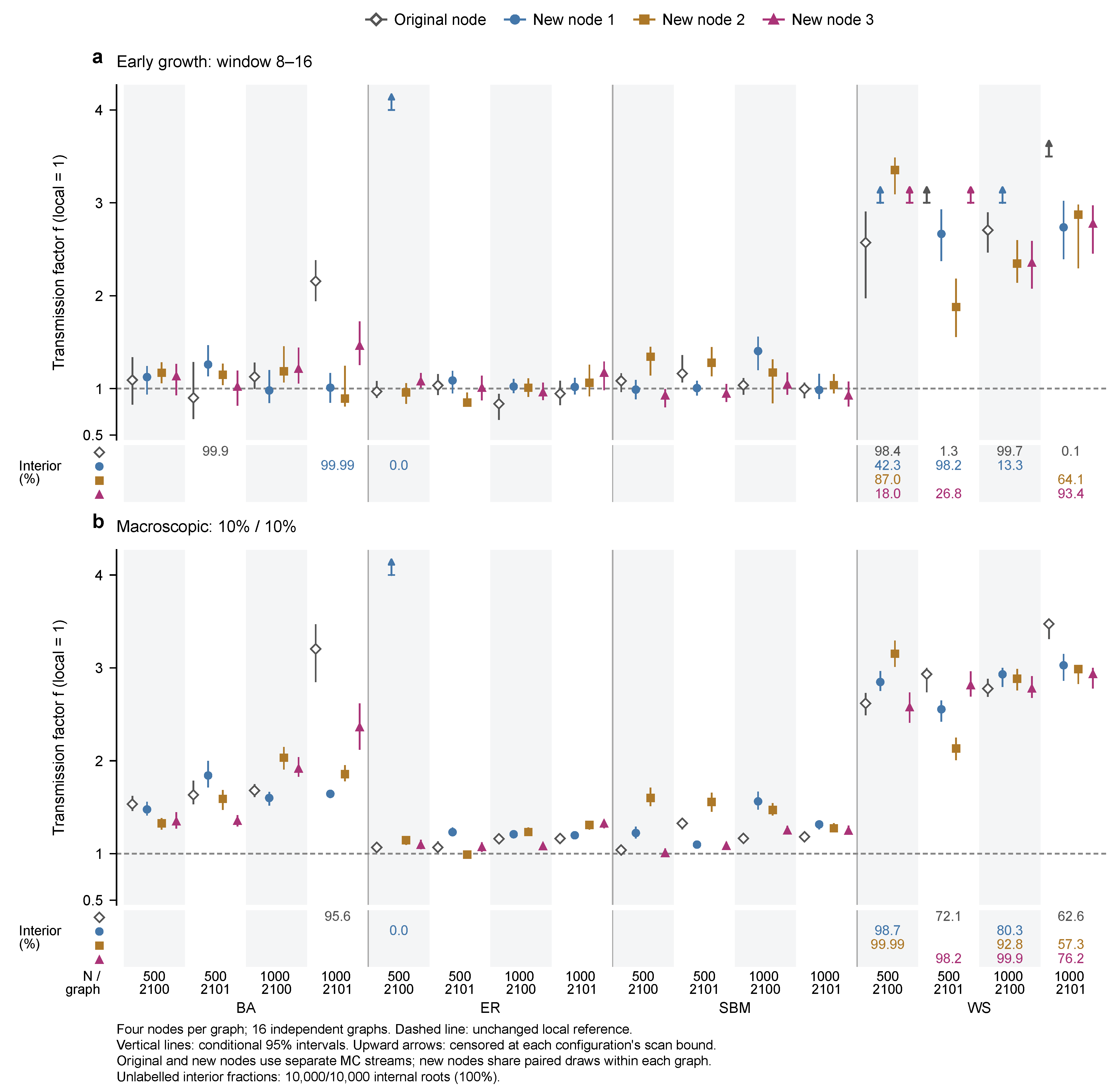
Appendix C. Recommendation-Parameter Sensitivity, DMP Validation, and Response Diagnostics
Appendix C.1. Recommendation-Parameter Sensitivity
The recommendation-parameter sensitivity experiment uses 40 registered networks (20 BA and 20 SBM, each with ). Figure A2 and Table A3 report Cumulative R4000, comprising the initial 800 and an independent addition of 3200 paired MC replicates per network and setting. The three modes share transmission, adoption, and deactivation streams. Recommendation-side consistency is permuted once per replicate, with that permutation reused across settings. The sensitivity baseline and six perturbations use random streams separate from those of the original four-mode experiment. Pilot and calibration trajectories are excluded. These baseline estimates complement, rather than replace, the original estimates in Section 5.2. Appendix C.2 describes the sampling stages. The complete Initial R800 figures and tables remain in the source data.
The response is final cumulative adoption fraction at , expressed in percentage points (pp). The baseline is . Six one-at-a-time perturbations give seven settings. Matched denotes the temporally budget-matched control and Shuffled denotes the shuffled-consistency control. Every effect is dynamic minus control. Pooled results summarize the same 40 networks, not an additional sample.
Let be the mean paired dynamic-minus-control difference on network n, setting s, and control c. Figure A2 reports . Table A3 reports , where 0 denotes the fresh baseline. Network-bootstrap draws resample within topology and jointly carry all settings and controls, preserving the network-level pairing. Pooled draws maintain the balanced 20:20 topology composition. All displayed intervals are pointwise 95% percentile intervals from 10,000 draws, conditional on the MC means. They do not account for all intervals simultaneously. No full factorial parameter interaction is estimated by the one-at-a-time design.
Table A3.
All 24 topology-specific paired parameter changes relative to baseline in Cumulative R4000. Positive changes indicate a larger dynamic-minus-control contrast than at baseline. They do not imply that the corresponding effect is positive or negative in absolute terms.
Figure A2.
Recommendation effects across parameter settings and network topologies. (a–c) Dynamic minus temporally budget-matched control. (d–f) Dynamic minus shuffled-consistency control. Columns vary , , or around the baseline . All other parameters remain fixed. Markers show medians of network-level effects. Error bars show pointwise 95% network-bootstrap intervals. The response is the final cumulative adoption fraction at , expressed in percentage points. BA and SBM each contribute 20 independent networks. The figure displays their 28 unique topology–setting–control summaries. The balanced-pooled summaries of these same 40 networks are retained in the source data. This display uses Cumulative R4000, averaging 4000 paired MC differences per network effect. The sampling stages and DMP validation are reported in Appendix C.2. The same baseline estimates recur in all three columns without adding observations. Horizontal offsets separate intervals, and straight segments guide the eye. Vertical scales differ between rows but are shared within a row. Parameter-response inference uses paired within-network changes (Table A3), not differences between plotted medians. The source data retain all 42 numerical effect estimates, intervals, and network sign counts.
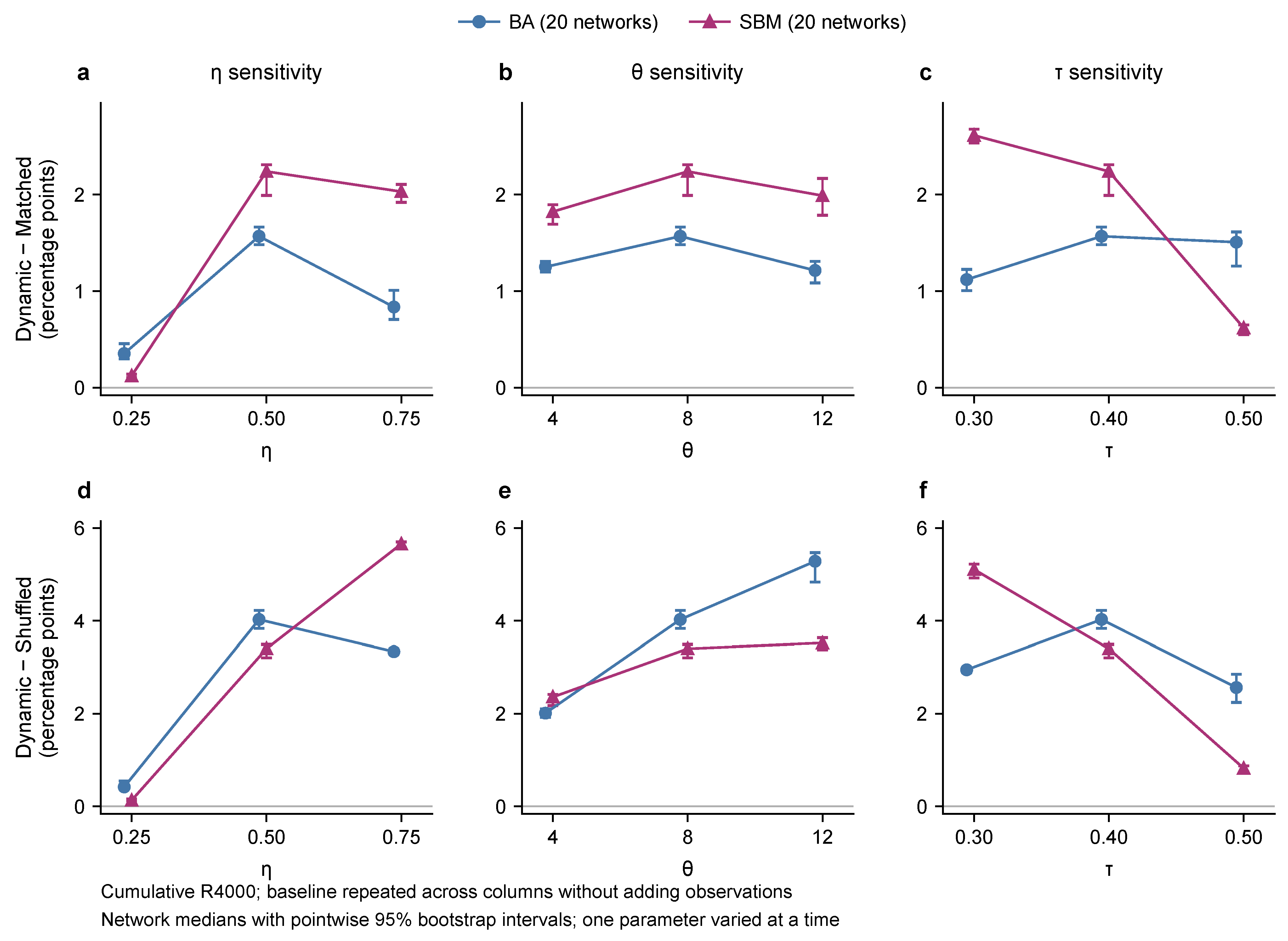
Appendix C.2. Fixed-Sample Precision Extension and DMP Parameter Validation
A separate variance calibration on eight registered graphs, seven settings and 100 replicates per cell set the initial fixed R800. Pilot and calibration trajectories were excluded from the formal samples.
After Initial R800, the variance-guided follow-up fixed an addition of 3200 independent-stream replicates per cell on the same forty networks and seven settings before new data collection. Pairing across modes and settings was retained. Independent R3200 supplies the new-batch estimate. Cumulative R4000 combines it with Initial R800. The source data retain the trajectory totals.
The 0.25-percentage-point MC half-width was a planning diagnostic, not a guarantee for every cell. Sampling stopped at the fixed sizes regardless of target attainment. Unconditional sequential coverage over the full variance-guided planning procedure has not been established.
All 42 topology-specific or balanced-pooled control-effect median intervals remained above zero in both added and cumulative MC stages, but not every parameter change was resolved. For versus 0.50, the cumulative BA dynamic-minus-shuffled change had eighteen negative and two positive network point estimates, compared with twenty negative points in R800. The two positive points had MC intervals spanning zero. The network median was pp (95% interval ). The cumulative SBM dynamic-minus-matched change had median pp and network interval , which spanned zero. The independent added batch likewise left this contrast unresolved. Full setting-effect and parameter-change summaries retain these exceptions.
The separate 560-condition DMP validation (Table 4) used the same predictions for all three MC-stage comparisons and was not pooled into the original 840-condition accuracy benchmark. Cumulative R4000 absolute endpoint error had a median of 0.763087, a 95th percentile of 1.751927, and a maximum of 2.354864 percentage points. These describe condition-level errors, not confidence limits. Figure A3a shows all 28 topology–setting–mode strata.
Define the adoption advantage G as dynamic minus temporally matched final adoption, and its response as . In SBM, the DMP response median was -0.393553 percentage points, whereas Independent R3200 and Cumulative R4000 MC had positive network-median responses and intervals (Table A4). Thus, the aggregate advantage-response directions were opposite in DMP and MC. This is not a reversal of total adoption. Both dynamic and matched adoption increased when decreased. Eighteen of the twenty DMP responses were negative, and eighteen cumulative MC responses were positive. All networks, including exceptions, are displayed in Figure A3b.
Table A4.
Separate sampling stages, MC precision, and SBM advantage-response estimates. R denotes the number of MC replicates per cell.
The precision target is a within-network MC 95% t half-width no greater than 0.25 percentage points. It is diagnostic and did not trigger extra sampling. Effect cells cover 40 networks × 7 settings × 2 controls, and response cells cover 40 networks × 6 non-baseline settings × 2 controls. Counts exclude duplicated balanced-pooled summaries. The last column is the pointwise percentile interval for the median of within-network changes on the twenty SBM graphs, conditional on estimated MC means. It is not an MC half-width. All stages use the same graphs, and Cumulative R4000 contains Initial R800 and Independent R3200, so the rows are not independent network samples. Figure A2 and Table A3 use Cumulative R4000. Complete Initial R800 estimates and displays, full 560-condition errors, and all 28 strata remain in the source data.
Figure A3.
Parameter-dependent endpoint errors and an effect-response mismatch. (a) All 28 topology–setting–mode summaries from the separate 560-condition DMP validation: 20 BA and 20 SBM networks, seven settings, and two modes (dynamic and temporally matched). Dots are medians of absolute DMP–MC endpoint error across 20 networks. Vertical segments extend to the 95th percentile. These segments describe error distributions, not confidence intervals. Filled circles and open squares denote dynamic and matched modes. Blue and purple denote BA and SBM. Base is , , . Each other setting changes one parameter. (b) All 20 SBM network responses of the dynamic-minus-matched adoption advantage when decreases from 0.4 to 0.3. Each point compares the MC-mean response with the corresponding deterministic DMP response on the same graph. Horizontal bars are the within-network MC 95% t intervals of the paired parameter change. Zero-reference lines identify response directions. They are not the network-bootstrap intervals in Table A4. Both panels use the Cumulative R4000 MC estimate at T = 100. Endpoint errors and advantage responses are in percentage points (pp). The effect response is a difference between recommendation modes, not a change in total adoption. The original 840-condition benchmark remains a separate population.
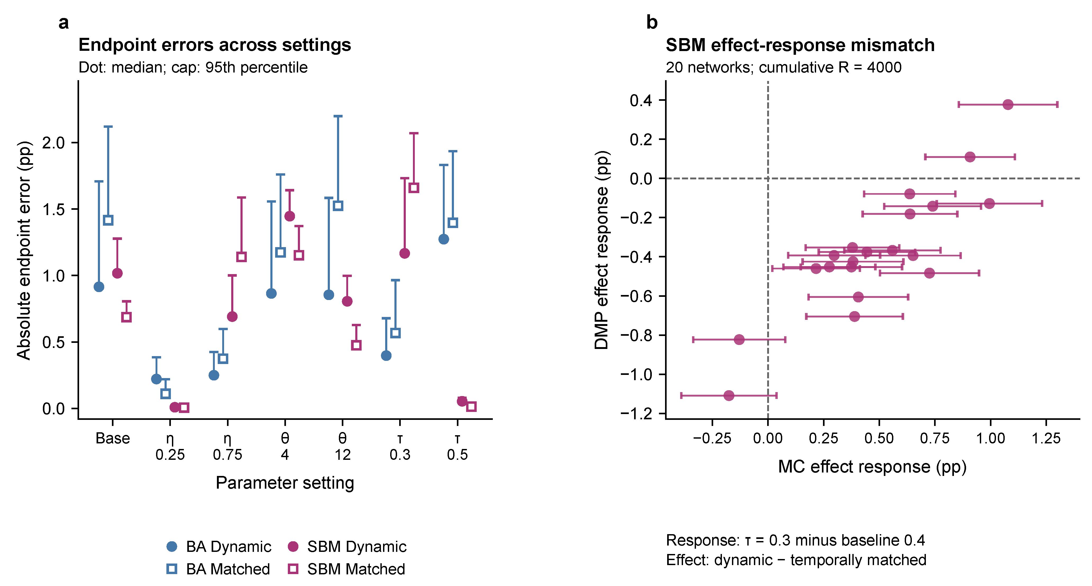
Table A5 reports all 240 paired advantage responses by topology and setting, including MC-unresolved cases.
Each row contains all 20 registered graphs of that topology. The 240 cells reuse forty graphs across six non-baseline settings, not 240 independent graphs. Medians summarize within-graph setting-minus-baseline changes in the dynamic-minus-matched advantage, not differences of marginal medians. Values are percentage points at .
Same and opposite directions require the paired MC setting-change 95% t interval to strictly exclude zero. Intervals containing or touching zero are MC unresolved and are not counted as DMP agreement. Exact-zero DMP responses with MC-resolved direction form a separate category, without a numerical sign tolerance. Direction agreement does not establish accurate response magnitude. The median columns are descriptive, not tests of network-level direction. The BA medians have opposite signs, while the MC network-median interval includes zero.
Table A5.
Complete descriptive classification of matched-advantage parameter responses against cumulative R4000 MC.
This post hoc classification uses existing pointwise intervals, not a new test family, simultaneous correctness rate or independent replication across settings. The complete Independent R3200 classification is retained in the source data. R3200 is part of Cumulative R4000, so the two summaries are not independent confirmations. Both complete 240-row source tables retain every response magnitude and its paired MC interval.
Appendix C.3. Matched-Control Design and Additive Error Decomposition
This diagnostic examined the previously observed SBM response disagreement when decreased from 0.40 to 0.30. It retained the twenty registered SBM graphs, stances, ten initial active nodes, , , , , , and . It was designed after the disagreement was observed. The outcome was cumulative adoption fraction, including the initial seeds.
Let U denote the original dynamic MC stream and its degree-weighted potential edge-opportunity budget path. The original matched control, C, used the same U and budget , and its endpoints were reused. Control A received the same but used an independent receiver stream V. Control B received the deterministic dynamic-DMP budget and the same V as A. Receiver streams were also shared across the two settings within each graph.
Write their endpoint fractions as , , and . Let be the saved matched and dynamic DMP predictions, and the dynamic MC endpoint. The registered decomposition was
Appendix C.4. Precision Stages and the Resolved Component
The first stage used 1000 driver realizations per graph and setting, followed by 2000 additional realizations with receiver streams independent of the first stage. The cumulative sample size was chosen from first-stage paired variances before the additional results were generated. Paired responses from both stages were combined, with cumulative variances retaining between-stage mean shifts rather than averaging standard errors. Both stages reused existing driver realizations. Replay did not create additional independent observations. The existing R4000 experiment remained an external reference.
The six primary responses in Table A6 were formed within each paired repeat. Fixed-network MC variance used with Satterthwaite t intervals, including joint driver–receiver randomness. The target was a pointwise 95% half-width of 0.10 percentage points for each response. Separate network intervals used 10,000 common graph resamples, conditional on the estimated MC means. Each primary family interval had nominal level . The cumulative intervals summarize uncertainty for the variance-guided fixed follow-up. Unconditional coverage over the full sequential design has not been established.
Table A6.
Matched-error response components and precision in Cumulative R3000. All numerical entries are percentage points. Network intervals use the six-comparison family. Full R1000 and additional R2000 half-widths remain in the source data.
The earlier stages did not meet all precision targets. Their complete results remain in the source data. Only Cumulative R3000 met the full criterion: and larger than both other components under the family MC intervals, with all three relevant precision targets met. Network-family intervals supported the same ordering. Cumulative was also positive under both interval families. The sign of and the ordering of versus remained unresolved under that family.
The cumulative matched-error increase was 0.9917 percentage points. Its signed mean-component shares were 91.10%, 3.81% and 5.09% for . These shares use the matched-error increase as the denominator, not the full allocation-advantage response error. The mean allocation-advantage responses remained positive for original C (+0.4985 pp), independent-receiver A (+0.4480 pp), and fixed-budget B (+0.4103 pp), whereas DMP predicted −0.3722 pp. Thus, removing shared driver randomness did not resolve this direction disagreement.
For the fixed external input, the expectation-level identity is , where is the unexposed probability. Finite MC estimates additionally have sampling error. Aggregate unexposed fractions cannot replace the adoption-weighted node quantities. This is an algebraic localization, not a causal allocation among graph structures. Original C lacked full saved trajectories, so and the complete three-component identity were evaluated only at . The source data retain every stage, failed precision check, interval and unresolved contrast.
Appendix C.5. Four Exact Comparisons on a Tree and a Merging-Path Motif
The fixed four-cell check compared the unchanged DMP with independent rational-probability enumeration under two externally prescribed budget pulses. It used nodes , with s initially active and all others unexposed. The directed tree had edges , , and . The diamond added . Adoption probabilities were , deactivation probability was 0.20, and . Total directed-edge budgets were zero except at updates 1 and 3, where they equaled either 1.2 or 2.4. Uniform visibility was budget divided by directed-edge count, giving the per-edge probabilities in Table A7. Exact enumeration retained UEAI states, adoption history and edge-success history, without pruning positive probability mass. No MC sampling was used.
Table A7.
Exact four-cell terminal results. Entries are adoption fractions, not percentage points. Fractions are retained exactly. No MC confidence intervals apply.
Both tree cells agreed in node states, cumulative adoption and edge messages. In both diamond cells, individual edge messages and the three upstream nodes also agreed. The target discrepancy matched the prespecified analytic prediction. With , and , the target incoming no-hit covariance is . The target exposure overestimate at time 4 is , and the network cumulative adoption overestimate from time 5 through 8 is . The initial source is already active, so its adoption probability is not multiplied again. Numerical agreement with the analytic discrepancies had maximum residual , below the fixed tolerance.
Under the prescribed budget pulses, this construction establishes loss of shared-ancestor dependence as a source of DMP closure error at a merging target, even without a directed cycle or triangle. Its contribution to error in the sampled SBM networks remains unquantified. The two graphs share total budgets but differ in edge counts and per-edge probabilities, so their absolute outcome difference is not a pure topology-effect estimate.
Appendix D. DMP Bias and Structural Diagnostics
Appendix D.1. Statistical Units and Analysis Scope
Appendix D.1, Appendix D.2, Appendix D.3, Appendix D.4 and Appendix D.5 reanalyze the original 840 method-comparable conditions, comprising 720 synthetic and 120 recommendation conditions from 160 independent network realizations. They add no diffusion simulations and do not incorporate the fresh recommendation-sensitivity simulations in Appendix C. The 40 replicate-wise shuffled MC conditions remain excluded from method-accuracy comparisons because their randomization level differs from that of the DMP extension. Graph, stance, and initial-state identities agree across the compared methods.
Signed error is . Positive values indicate overestimation. Relative absolute error is . No denominator is zero. Fractions are converted to percentage points (pp) by multiplication by 100, whereas relative absolute errors are expressed as percentages. The independent resampling unit is the network. Conditions sharing a network, including transmission factors and feedback layers, remain together in each of 10,000 bootstrap draws. Resampling is stratified by experimental family, topology, and size. The 2.5th and 97.5th percentiles give pointwise intervals for the condition-weighted mean or median. These intervals condition on the stored MC means and do not include a second MC-replicate resampling layer.
The family of 12 two-sided exact sign tests was specified in the revision plan before this added analysis, after the original descriptive bias results were available. It was not an original preregistration. For each topology and at , the two feedback-layer signed errors are averaged within each network, giving 20 independent values. The null assigns equal probabilities to positive and negative values. Exact zeros are counted separately and omitted from the binomial sample. Holm correction covers all 12 tests. These tests concern error direction within a design stratum, not differences between topologies or significance of each of the 840 conditions.
Feedback contrasts use for 360 network–factor pairs from 120 networks. For the WS transmission contrast, the two feedback layers are averaged within each network before taking the error at minus that at . Network-block resampling retains all factors for these paired contrasts. The bootstrap base seed was 20261010, with recorded table-specific derived seeds. Software versions are given in Appendix F.1.
Appendix D.2. Complete Stratified Errors and Network-Level Tests
The overall mean signed error was 0.008001 (95% interval, 0.007621–0.008386), or 0.8001 percentage points. The overall median signed error and its interval are reported in Section 5.1. Table A8 and Table A9 report all 42 observed strata from 840 conditions on 160 independent networks, with 20 networks per row and the same networks recurring across rows. In the SBM weak-visibility stratum, the median signed error is negative, and the interval for the mean signed error spans zero. P95 denotes the 95th percentile of absolute condition errors, not a confidence limit.
In Table A8, .
Table A8.
DMP final-size errors in the synthetic benchmark. Active and no heat denote active-prevalence feedback and , respectively. The displayed mean intervals are pointwise network-bootstrap intervals. No MC scale comparison is available at for ER or WS.
Table A9.
DMP final-size errors in the method-comparable recommendation benchmark. All networks have and . For SBM with weak visibility, the median signed error is −0.0272 pp, and the interval for the mean signed error spans zero. Full signed-median values remain in the source data.
Table A10.
All 12 network-level sign tests, grouped by identical results. Each test uses 20 independent synthetic networks at , after averaging the two feedback-layer errors within each network. Counts and p-values apply separately to each listed stratum. All 12 tests retain their separately computed results and the original 12-test Holm family. The raw and Holm-adjusted values are rounded from the saved exact calculations. All 12 reject the equal-sign-probability null at . No between-topology test is implied.
Appendix D.3. Paired Feedback and Transmission Contrasts
Across all 360 pairs, the mean feedback contrast was (95% interval, ). The WS mean was positive, whereas the other five topology–size means were negative (Figure A4c). The directions refer to averages over the three factors and do not assert an identical response in every condition. The WS versus contrast was positive in all 20 networks, with median 0.025879 (0.021955–0.029229). Section 5.1 reports its mean and interval.
Figure A4.
DMP bias, paired feedback contrasts, and WS structural intervention. (a) Mean signed final-adoption bias, DMP minus MC at , across the original 840 conditions from 160 independent networks. S denotes synthetic benchmarks (filled circles, six conditions per network). R denotes recommendation benchmarks (open squares, three conditions per network). Each row contains 20 networks. (b) Bias by transmission factor for synthetic networks, averaging both feedback layers within each of 20 networks per point. Lines guide the eye. (c) Active-feedback minus no-heat bias for 360 network–factor pairs from 120 networks. Each row contains 20 networks and 60 pairs. (d) Mean structural contrast D for twenty WS graph pairs, with both structures evaluated at the original graph’s fixed actual transmission levels. All bias and effect axes use percentage points. Panel (b)’s horizontal axis is the normalized transmission factor. Intervals in (a–c) remain pointwise 95% network-block percentiles. (d) uses 97.5% percentiles for each of two primary contrasts, giving nominal 95% family coverage. All panels use 10,000 network resamples and condition on saved MC means. Panel (d)’s separately evaluated MC half-widths are reported in Appendix D.6 and are not combined with its network intervals. No between-topology hypothesis test is displayed.
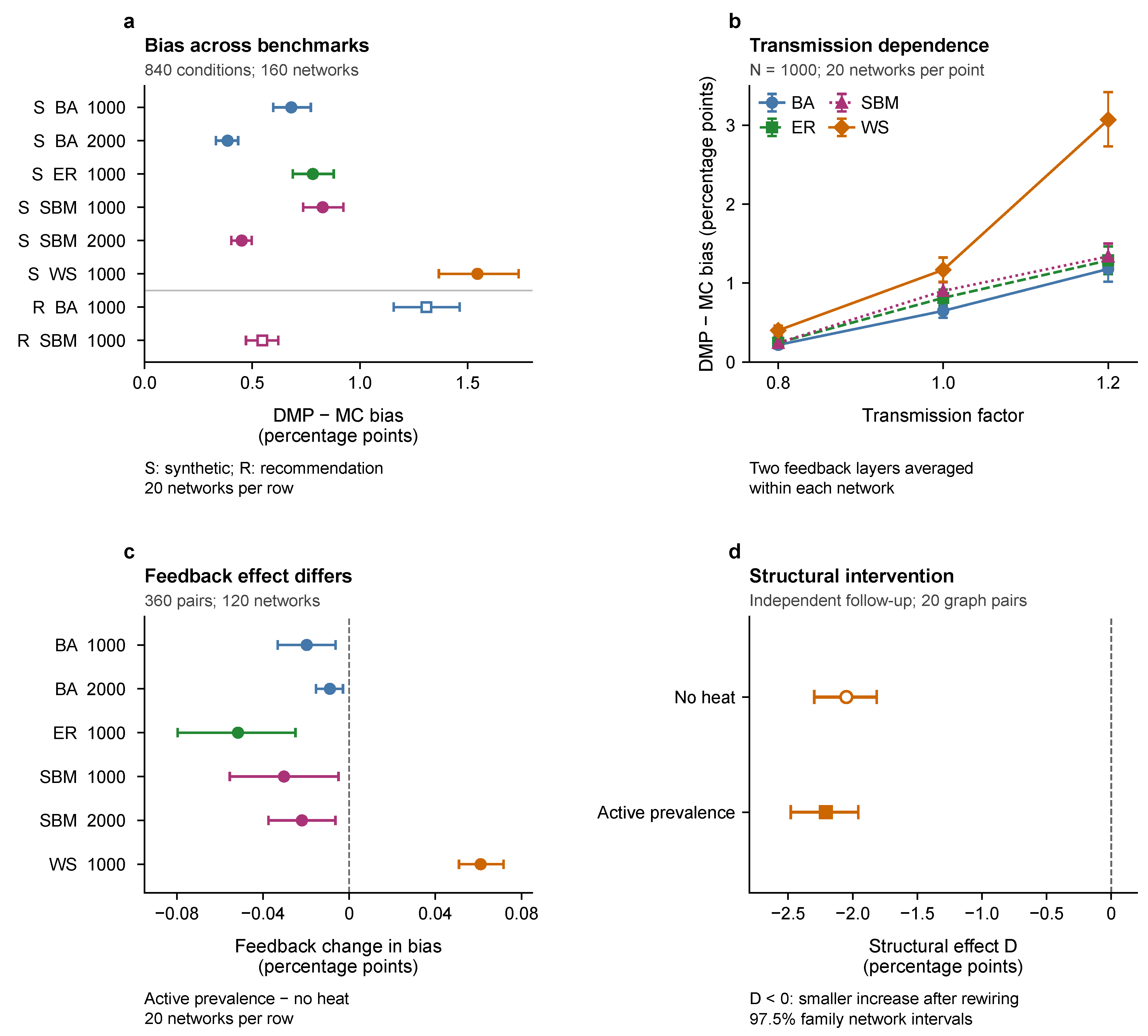
Appendix D.4. Exploratory Structural Associations
Within the twenty sampled WS networks at and , the exploratory correlations did not establish an increasing relation between clustering or four-cycles and signed DMP error. The clustering coefficient ranged from 0.4614 to 0.4860. The structural metrics were not manipulated independently and may covary, so these observations neither identify a unique cause nor rule out contributions from short cycles and overlapping paths. Full results for all 108 correlations, their methods and the original six-metric WS table are retained in the source data. The degree-preserving intervention is reported separately in Appendix D.6.
Appendix D.5. MC Precision, Common Endpoint, and Source Data
All 840 stored MC summaries met the original precision criterion, with final-size interval half-widths ranging up to 0.007954 and a median of 0.003591. These marginal intervals characterize MC sampling precision separately from the network-bootstrap intervals. They are not simultaneous intervals for all benchmark conditions.
Endpoint checks cover 2400 method conditions from the original accuracy benchmark (840 DMP, 840 MC, and 720 MMCA), separately from later independent follow-up experiments. DMP and MC cover the same conditions. MMCA covers the method-comparable subset. At , cumulative adoption matches each method’s stored summaries. The maximum increments from to were 0.002893 for DMP, 0.001063 for MC, and 0.007844 for MMCA. Residual exposed and active fractions and the final-step increments are retained in the source data. This is a comparison at a common finite endpoint, not a claim that every trajectory has reached absorption. A residual state fraction is not an upper bound on subsequent cumulative adoption.
The retained records include the 840 condition-level errors, all stratum summaries, the 12 exact tests, 360 feedback pairs, 20 WS transmission contrasts, 160 network structures, all 108 structural correlations, and endpoint diagnostics.
Appendix D.6. Degree-Preserving WS Structural Intervention
The structural follow-up reused the twenty WS benchmark graphs. One call to NetworkX 3.3’s connected double-edge-swap procedure requested swap attempts per graph, where M is its undirected edge count. This specifies attempts, not a guaranteed count of successful swaps. No graph was replaced or topped up. Node labels, each node’s degree, connectedness, stances, adoption/deactivation probabilities, and the original initial active set were preserved. Actual transmission levels were fixed from the original graph at and . Both structures and feedback layers used these same levels and .
Each of the 160 conditions used 2000 fresh MC trajectories and one DMP calculation, giving 320,000 trajectories. The primary estimand in each feedback layer was the equally weighted mean across twenty original graph pairs:
Within a structure, common streams paired transmission levels and feedback layers. Streams were independent between structures. MC variance used paired high-minus-low replicate differences within structure, combining independent structures and graphs with equal graph weights. Satterthwaite t intervals quantified MC uncertainty on these fixed graph pairs. Network-bootstrap intervals used 10,000 common graph-index draws carrying both structures, levels, and feedback layers. They conditioned on the MC means. Each of the two prespecified primary contrasts used a 97.5% interval for Bonferroni family-level 95% coverage, separately for MC and network uncertainty.
Both contrasts were negative under both uncertainty assessments (Figure A4d). Their ordinary MC 95% half-widths were 0.0325 and 0.0347 percentage points, below the frozen 0.10-point target. At high transmission, mean absolute error fell from 3.024 to 0.627 percentage points without feedback and from 3.157 to 0.581 with feedback. The no-feedback potential edge-opportunity budgets were identical after rewiring because per-node degrees and visibilities were preserved. With active feedback, budgets followed each structure’s own trajectory and were not externally matched.
The layer contrast had a conservative fixed-graph MC interval below zero, but its network interval included zero. These intervals were formed from the corresponding family bounds.
The intervention establishes a reduction in error growth under joint structural change. It does not isolate clustering, short cycles, path length, or feedback-closure contributions. All reported endpoint comparisons concern the frozen horizon.
Appendix D.7. Temporal Prediction Diagnostics
Complete-trajectory diagnostics use all 840 original method-comparable DMP–MC condition pairs in Section 5.1. Dynamic-peak timing uses the 291 conditions with . The remaining 549 conditions have an initial peak. The reported percentiles describe condition-level absolute errors, not confidence intervals.
Peak-time errors varied across topologies and transmission conditions. Among dynamic-peak conditions, the 95th percentile of absolute peak-time error ranged from 2.4 to 6.95 time steps across topology–experiment strata. In the synthetic-diffusion subset, it was 8.55 and 5 time steps at normalized transmission levels 1.0 and 1.2, respectively, whereas level 0.8 produced no dynamic peaks.
Appendix E. Operational-Root Uncertainty and Independent WS Localization
Appendix E.1. Early-Growth Root Uncertainty in the Registered 80-Network Experiment
The uncertainty analysis used 506,400 reconstructed MC trajectories, rather than trajectories recovered from the original files. The point roots and states in all 240 network–window combinations reproduced the originally reported values. The maximum absolute difference between internal normalized roots was .
Within each network, 10,000 bootstrap draws resampled complete 25-time-point exposed-plus-active trajectories, including extinction. Replicate indices were grouped by their availability across factors, and the same weights were applied within each group to all its factors and time points. This retained all realized factor-specific sample sizes. The three observation windows shared each draw. We preserved the original exact-zero/first-sign-bracket estimator without smoothing the growth curve. Invalid factors, multiple crossings, and all censoring states were recorded.
Percentiles were calculated only among internal roots. They therefore describe conditional root location, not the probability of identifying a root or the unconditional coverage of a confidence procedure incorporating adaptive stopping. The internal-root fraction must be read alongside each interval. The 80% threshold below is a descriptive count, not an exclusion or significance rule.
Figure A5.
Operational-root uncertainty, censoring and root availability in the original 80-network experiment. (a) All 80 point estimates in the primary 8–16 window. Dots denote internal roots, vertical lines their conditional 2.5th–97.5th bootstrap percentiles, and orange upward arrows the upper scan bounds of the ten right-censored points. A censored point is not replaced by an internal-bootstrap percentile. The dashed line denotes the deterministic local reference, . (b) Internal-root fractions for all 240 network–window combinations, using a linear 0–100% color scale. Columns list network seeds 2100–2109 within each topology–size stratum. The heatmap rows denote the three growth windows. Each network contributes 10,000 joint factor/window resamples. Networks, not individual trajectories, are the independent network realizations. No hypothesis test is used. Conditional percentiles based on very few internal draws cannot establish precise localization.
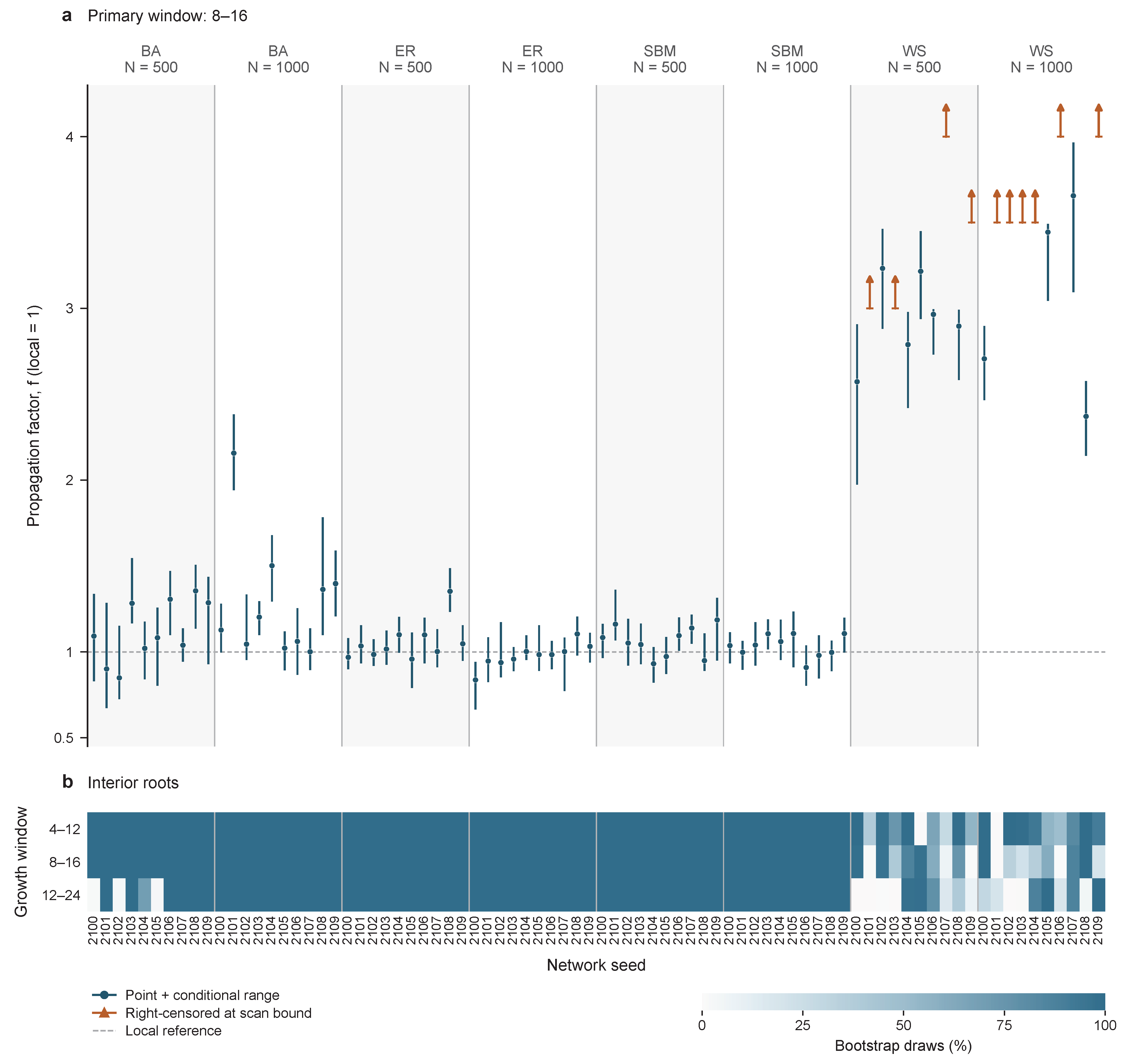
For the main window, all BA, ER, and SBM strata had median internal-root fractions of 1.0000, whereas the WS median was 0.5041. 13/20 WS fractions were below 0.80. Across all windows, 182/240 cells exhibited multiple raw sign crossings in at least one of their 10,000 bootstrap draws. The registered first-root rule selects an operational root without establishing uniqueness. Full crossing frequencies are retained in the source data. Conditional percentile spans based on rare internal roots in censored cells were retained in the source data but were not plotted as well-identified point-root intervals.
The local spectral reference is deterministic conditional on the graph and parameters. Its numerical residual is distinct from MC sampling uncertainty. The maximum audited spectral residual across the 80 networks was . The macroscopic intervals and their distinct resampling units are specified in Section 4.4. Full point estimates, all bootstrap states and diagnostics, and the per-network intervals are retained in the source data.
Appendix E.2. Independent Fixed-Sample WS Localization
The follow-up selected the 31 configurations containing an unmet target in the preceding fixed-R2000 WS stage: 42 targets and 20 companion endpoints give 62 primary endpoints on twenty graphs. The complete earlier-stage accounting remains in the source data. This study is distinct from the sixteen-graph seed experiment in Appendix B.3.
The follow-up fixed the complete factor grid and –31,400 per configuration before additional simulations. The twenty graphs comprised ten at each size. Configurations and MC repeats did not add independent graphs. Feedback was disabled, with one initial active node and . Old MC samples were not pooled. Each configuration generated 10,000 bootstrap draws from its registered bootstrap seed, retaining its complete sample of R trajectories. One weight vector jointly resampled its factors and nine endpoints. Different configurations used independent streams and weights, without truncation to a common R.
All 62 primary point roots were internal, with bootstrap internal-root fractions of 1 and qualifying brackets. The full three-part precision rule was met by 30/42 prior targets and 50/62 primary endpoints (Table A11). The twelve failures were early-growth roots (four at and eight at ) with conditional interval widths of – on the normalized f-axis. All 62 primary pointwise conditional intervals lay above . The smallest lower bound among the failures was . These intervals support separation from the local reference despite unmet width targets, without a simultaneous confidence guarantee. Sampling stopped at the fixed sizes and grid.
The nine endpoints per configuration yield 279 estimates, comprising 62 primary and 217 secondary endpoints (Table A11). The two primary definitions and 42 unmet targets were selected before follow-up sampling. Of 217 secondary endpoints, 180 missed at least one precision criterion or were point-censored. A narrow bootstrap interval conditions on the sampled grid and interpolation rule and cannot compensate for a coarse bracket. Additional repeats at unchanged factors do not refine that bracket.
Each endpoint is counted once. Pass requires an internal-root bootstrap fraction of at least 0.95, a conditional 95% interval full width at most 0.20, and point-bracket width at most 0.05 (the registered tolerance applies to bracket comparison). Both widths are measured on the normalized f-axis. Internal, unqualified denotes an internal point root that fails at least one of these criteria. Point estimates classified as right-censored occupy the final column irrespective of whether some bootstrap draws produced an internal root. The original bracket-only, width-only and multiple-criteria classifications are preserved in the source data.
For target probability 0.5, all 93 macro endpoints missed the complete localization criterion: 36 point roots were internal but insufficiently resolved, and 57 were right-censored. The latter had empirical event probabilities below 0.5 at the registered upper limit .
Table A11.
Precision diagnostics for all retained WS endpoints. Each of the nine endpoint definitions is evaluated on the same 31 configurations, with 15 configurations at and 16 at . Size-specific prior-target accounting remains in the source data. Macro labels give coverage q/target probability . Primary endpoints are early growth over 8–16 and macro 0.1/0.1. Subtotal and overall n values count endpoints.
Right censoring means that the registered estimator did not locate an internal root in the evaluated domain. It does not establish whether the true event probability reaches 0.5. The complete bootstrap breakdown is retained in the source data. We neither replace censored roots by scan limits nor use conditional intervals from rare internal draws as precise locations. The original eighty-network Table A2 remains a separate stage. Its internal-root medians under different criteria need not involve the same available networks and are not interpreted as paired within-network effects.
The independent WS seed and window comparisons are separate from the original 16-graph seed-sensitivity experiment in Appendix B.3. The 42 seed comparisons involve 21 node pairs within four graphs. The 62 window comparisons involve 31 configurations on twenty graphs. Within each configuration, the 8–16 early-growth root is subtracted from the 4–12 and 12–24 roots. Seed differences combine independent configuration draws at each full R. Window differences use shared within-configuration draws. All pointwise 95% difference intervals condition on both roots being internal.
Seed-difference intervals exclude zero in 20/21 early-growth and 18/21 macroscopic comparisons. Table A12 summarizes all comparisons by precision stratum, including the four seed and twelve window comparisons whose intervals do not exclude zero.
Table A12.
Existing seed and window comparisons stratified descriptively by endpoint precision. Entries give the number of pointwise 95% conditional difference intervals excluding zero/the number of comparisons in that row.
Table A12’s precision-qualified strata require both roots to pass either all Table A11 criteria or the bracket-width criterion alone. These overlapping subsets of dependent comparisons are descriptive. Their counts are read separately.
Precision qualification matters: 21 of the 50 window intervals excluding zero involve at least one coarse point bracket. Thus, 50/62 summarizes conditional differences on the frozen grid. Finer localization is assessed separately in Table A12.
Joint internal-root availability and whether a conditional difference interval excludes zero describe different aspects of uncertainty. Table A12 keeps and 1000 separate. These two sizes do not establish a finite-size scaling law or an effect distribution over all possible seeds.
Forty early-growth endpoints had more than one crossing in at least one saved bootstrap draw, with maximum frequency 1.19%. The operational root rule does not establish uniqueness.
Appendix F. Implementation and Reproducibility
Appendix F.1. Implementation and Matched Inputs
Calculations used Python 3.12.7. The common inputs and comparison populations are specified in Section 4.2 and Section 4.3 and Table 4. Budget-matched controls use the corresponding method’s dynamic trajectory. MC matching is performed separately within each replicate. Analysis data, figure source data and code are retained with the full software environment, configuration and seed registries, experiment and analysis entry points, and provenance records. These materials are available from the corresponding author upon reasonable request.
Appendix F.2. Synchronous Update Procedure
The following pseudocode specifies one MC trajectory. All state tests in an update refer to the state at time t.
- Input: graph, node adoption probabilities, deactivation probability mu, fixed initial state,
- recommendation parameters, endpoint T = 100, registered replicate seed.
- Generate independent uniform arrays for every time-edge exposure trial,
- every time-node adoption trial, and every time-node deactivation trial.
- Set C(0) to the number of initially active nodes; record the initial state.
- For t = 0, …, T - 1:
- Compute H(t) from the current active fraction, or set H(t) = 0
- for the no-feedback setting; evaluate target visibility r_i(t).
- For each edge j -> i whose source is active at t, compare its exposure
- draw with lambda * r_i(t). Mark each unexposed target hit at least once.
- For nodes exposed at t, compare adoption draws with beta_i.
- For nodes active at t, compare deactivation draws with mu.
- Commit all transitions together: hit U -> E; adopting E -> A;
- rejecting E -> I; deactivating A -> I; otherwise retain the state.
- Increase C by the number of E -> A transitions and record time t + 1.
- Return the state trajectories, cumulative adoption, and peak quantities.
Newly exposed nodes cannot adopt until the next update. Newly active nodes cannot transmit or deactivate in the same update. An active source can transmit during its deactivation update. Model parameters and recommendation controls follow Section 2.1, Section 2.2 and Section 2.3.
Appendix F.3. Randomization and Replicate Counts
Seeds for graph generation, stances, initial states, and MC trials are recorded separately. Pairing reuses exposure, adoption, and deactivation draws at fixed time–edge or time–node indices. Each original control shares a stream with its own dynamic reference. Different control contrasts need not share a stream.
Recommendation sensitivity shares random streams across modes and all seven settings within each network. The shuffled control uses one recommendation-side permutation per replicate, shared across settings. Added batches use independent streams. The three new seed positions share streams across nodes and factors within each graph, while original-seed references have separate streams. WS structural comparisons share streams across transmission and feedback settings within each structure, with independent streams between structures. WS localization shares streams and bootstrap weights across factors and windows within a configuration. Configurations use independent streams and weights and retain their full respective sample sizes. Matched-diagnostic pairing is specified in Appendix C.3. Exact seed derivations and registries are retained in the reproducibility records.
Table A13 summarizes the Monte Carlo sampling rules and replicate counts.
Table A13.
Monte Carlo sampling rules and replicate counts.
The stopping rules determine the number of MC trajectories, while the MC observation endpoint remains at . Table 4 identifies the network populations and repeated conditions. Variance-guided follow-ups are subsequent stages planned from earlier results. Their sampling and uncertainty interpretation are detailed in Appendix C.2, Appendix E.2 and Appendix C.4.
References
- Alfaifi, Y.H. Recommender systems applications: Data sources, features, and challenges. Information 2024, 15, 660. [Google Scholar] [CrossRef] [Scilit]
- Huszár, F.; Ktena, S.I.; O’Brien, C.; Belli, L.; Schlaikjer, A.; Hardt, M. Algorithmic amplification of politics on Twitter. Proc. Natl. Acad. Sci. USA 2022, 119, e2025334119. [Google Scholar] [CrossRef] [Scilit]
- Pathak, R.; Spezzano, F.; Pera, M.S. Understanding the contribution of recommendation algorithms on misinformation recommendation and misinformation dissemination on social networks. ACM Trans. Web 2023, 17, 35:1–35:26. [Google Scholar] [CrossRef] [Scilit]
- Guess, A.M.; Malhotra, N.; Pan, J.; Barberá, P.; Allcott, H.; Brown, T.; Crespo-Tenorio, A.; Dimmery, D.; Freelon, D.; Gentzkow, M.; et al. How do social media feed algorithms affect attitudes and behavior in an election campaign? Science 2023, 381, 398–404. [Google Scholar] [CrossRef] [Scilit]
- Ullah, F.; Lee, S. Social content recommendation based on spatial-temporal aware diffusion modeling in social networks. Symmetry 2016, 8, 89. [Google Scholar] [CrossRef] [Scilit]
- Chaney, A.J.B.; Stewart, B.M.; Engelhardt, B.E. How algorithmic confounding in recommendation systems increases homogeneity and decreases utility. In Proceedings of the 12th ACM Conference on Recommender Systems, Vancouver, BC, Canada, 2–7 October 2018; ACM: New York, NY, USA, 2018; pp. 224–232. [Google Scholar] [CrossRef] [Scilit]
- Fabbri, F.; Croci, M.L.; Bonchi, F.; Castillo, C. Exposure inequality in people recommender systems: The long-term effects. Proc. Int. AAAI Conf. Web Soc. Media 2022, 16, 194–204. [Google Scholar] [CrossRef] [Scilit]
- Mansoury, M.; Abdollahpouri, H.; Pechenizkiy, M.; Mobasher, B.; Burke, R. Feedback loop and bias amplification in recommender systems. In Proceedings of the 29th ACM International Conference on Information and Knowledge Management, Virtual Event, Ireland, 19–23 October 2020; ACM: New York, NY, USA, 2020; pp. 2145–2148. [Google Scholar] [CrossRef] [Scilit]
- Zeng, A.; Yeung, C.H.; Medo, M.; Zhang, Y.-C. Modeling mutual feedback between users and recommender systems. J. Stat. Mech. Theory Exp. 2015, 2015, P07020. [Google Scholar] [CrossRef] [Scilit]
- Jiang, W.; Gao, X.; Xu, G.; Chen, T.; Yin, H. Challenging low homophily in social recommendation. In Proceedings of the ACM Web Conference 2024, Singapore, 13–17 May 2024; ACM: New York, NY, USA, 2024; pp. 3476–3484. [Google Scholar] [CrossRef] [Scilit]
- Bakshy, E.; Messing, S.; Adamic, L.A. Exposure to ideologically diverse news and opinion on Facebook. Science 2015, 348, 1130–1132. [Google Scholar] [CrossRef] [Scilit]
- Del Vicario, M.; Bessi, A.; Zollo, F.; Petroni, F.; Scala, A.; Caldarelli, G.; Stanley, H.E.; Quattrociocchi, W. The spreading of misinformation online. Proc. Natl. Acad. Sci. USA 2016, 113, 554–559. [Google Scholar] [CrossRef] [Scilit]
- Vosoughi, S.; Roy, D.; Aral, S. The spread of true and false news online. Science 2018, 359, 1146–1151. [Google Scholar] [CrossRef] [Scilit]
- Cinelli, M.; De Francisci Morales, G.; Galeazzi, A.; Quattrociocchi, W.; Starnini, M. The echo chamber effect on social media. Proc. Natl. Acad. Sci. USA 2021, 118, e2023301118. [Google Scholar] [CrossRef] [Scilit]
- Sun, M.; Ma, X.; Huo, Y. Does social media users’ interaction influence the formation of echo chambers? Social network analysis based on vaccine video comments on YouTube. Int. J. Environ. Res. Public Health 2022, 19, 15869. [Google Scholar] [CrossRef] [Scilit]
- Li, M.; Wang, X.; Gao, K.; Zhang, S. A survey on information diffusion in online social networks: Models and methods. Information 2017, 8, 118. [Google Scholar] [CrossRef] [Scilit]
- Firdaniza, F.; Ruchjana, B.N.; Chaerani, D.; Radianti, J. Information diffusion model in Twitter: A systematic literature review. Information 2022, 13, 13. [Google Scholar] [CrossRef] [Scilit]
- Kempe, D.; Kleinberg, J.; Tardos, É. Maximizing the spread of influence through a social network. In Proceedings of the Ninth ACM SIGKDD International Conference on Knowledge Discovery and Data Mining, Washington, DC, USA, 24–27 August 2003; ACM: New York, NY, USA, 2003; pp. 137–146. [Google Scholar] [CrossRef] [Scilit]
- Moreno, Y.; Nekovee, M.; Pacheco, A.F. Dynamics of rumor spreading in complex networks. Phys. Rev. E 2004, 69, 066130. [Google Scholar] [CrossRef] [Scilit]
- Barabási, A.-L.; Albert, R. Emergence of scaling in random networks. Science 1999, 286, 509–512. [Google Scholar] [CrossRef] [Scilit]
- Erdos, P.; Rényi, A. On random graphs. I. Publ. Math. Debr. 1959, 6, 290–297. [Google Scholar] [CrossRef] [Scilit]
- Holland, P.W.; Laskey, K.B.; Leinhardt, S. Stochastic blockmodels: First steps. Soc. Netw. 1983, 5, 109–137. [Google Scholar] [CrossRef] [Scilit]
- Watts, D.J.; Strogatz, S.H. Collective dynamics of “small-world” networks. Nature 1998, 393, 440–442. [Google Scholar] [CrossRef] [Scilit]
- Newman, M.E.J. Assortative mixing in networks. Phys. Rev. Lett. 2002, 89, 208701. [Google Scholar] [CrossRef] [Scilit]
- Fu, G.; Liang, H. The influence of core-periphery structure on information diffusion over social networks. Mathematics 2025, 13, 3048. [Google Scholar] [CrossRef] [Scilit]
- Kim, M.; Newth, D.; Christen, P. Modeling dynamics of diffusion across heterogeneous social networks: News diffusion in social media. Entropy 2013, 15, 4215–4242. [Google Scholar] [CrossRef] [Scilit]
- Gleeson, J.P.; Cellai, D.; Onnela, J.-P.; Porter, M.A.; Reed-Tsochas, F. A simple generative model of collective online behavior. Proc. Natl. Acad. Sci. USA 2014, 111, 10411–10415. [Google Scholar] [CrossRef] [Scilit]
- Wang, Y.; Cui, M.; Liu, M.; Wang, C.; Wang, Q. Dynamical analysis of an I2EH2S2R information spreading model with opinion divergence. Comput. Appl. Math. 2025, 44, 143. [Google Scholar] [CrossRef] [Scilit]
- Liu, X.; Li, T.; Xu, H.; Liu, W. Spreading dynamics of an online social information model on scale-free networks. Phys. A 2019, 514, 497–510. [Google Scholar] [CrossRef] [Scilit]
- Ding, J.; Li, Z.; Wu, X.; Liu, R.; Hu, H. Information dissemination model based on social networks characteristics. Mathematics 2025, 13, 1254. [Google Scholar] [CrossRef] [Scilit]
- Tong, X.; Jiang, H.; Chen, X.; Yu, S.; Li, J. Dynamic analysis and optimal control of rumor spreading model with recurrence and individual behaviors in heterogeneous networks. Entropy 2022, 24, 464. [Google Scholar] [CrossRef] [Scilit]
- Maojie, R. URU-SIS: A model for information propagation in multiplex networks. Chaos Solitons Fractals 2026, 204, 117788. [Google Scholar] [CrossRef] [Scilit]
- Hong, Z.; Zhou, H.; Wang, Z.; Yin, Q.; Liu, J. Coupled propagation dynamics of information and infectious disease on two-layer complex networks with simplices. Mathematics 2023, 11, 4904. [Google Scholar] [CrossRef] [Scilit]
- Bi, J.; Sun, N. Epidemic spreading and control on preferential attachment hypergraph with community. Mathematics 2026, 14, 2703. [Google Scholar] [CrossRef] [Scilit]
- Granell, C.; Gómez, S.; Arenas, A. Dynamical interplay between awareness and epidemic spreading in multiplex networks. Phys. Rev. Lett. 2013, 111, 128701. [Google Scholar] [CrossRef] [Scilit]
- Jankowski, R.; Chmiel, A. Role of time scales in the coupled epidemic-opinion dynamics on multiplex networks. Entropy 2022, 24, 105. [Google Scholar] [CrossRef] [Scilit]
- Bartal, A.; Jagodnik, K.M. Role-aware information spread in online social networks. Entropy 2021, 23, 1542. [Google Scholar] [CrossRef] [Scilit]
- Perra, N.; Rocha, L.E.C. Modelling opinion dynamics in the age of algorithmic personalisation. Sci. Rep. 2019, 9, 7261. [Google Scholar] [CrossRef] [Scilit]
- Gausen, A.; Luk, W.; Guo, C. Using agent-based modelling to evaluate the impact of algorithmic curation on social media. J. Data Inf. Qual. 2023, 15, 2:1–2:24. [Google Scholar] [CrossRef] [Scilit]
- Pescetelli, N.; Barkoczi, D.; Cebrian, M. Bots influence opinion dynamics without direct human-bot interaction: The mediating role of recommender systems. Appl. Netw. Sci. 2022, 7, 46. [Google Scholar] [CrossRef] [Scilit]
- Bagnoli, F.; Cvetković, T.J.; Guazzini, A.; Lió, P.; Romei, R. Modeling the spreading of fake news through the interactions between human heuristics and recommender systems. Information 2026, 17, 314. [Google Scholar] [CrossRef] [Scilit]
- Karrer, B.; Newman, M.E.J. Message passing approach for general epidemic models. Phys. Rev. E 2010, 82, 016101. [Google Scholar] [CrossRef] [Scilit]
- Lokhov, A.Y.; Mézard, M.; Zdeborová, L. Dynamic message-passing equations for models with unidirectional dynamics. Phys. Rev. E 2015, 91, 012811. [Google Scholar] [CrossRef] [Scilit]
- Karrer, B.; Newman, M.E.J.; Zdeborová, L. Percolation on sparse networks. Phys. Rev. Lett. 2014, 113, 208702. [Google Scholar] [CrossRef] [Scilit]
- Isham, V.; Kaczmarska, J.; Nekovee, M. Spread of information and infection on finite random networks. Phys. Rev. E 2011, 83, 046128. [Google Scholar] [CrossRef] [Scilit]
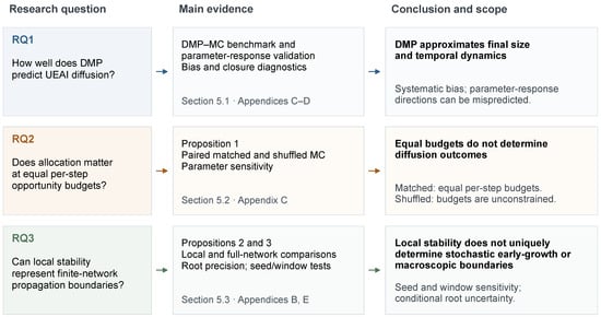
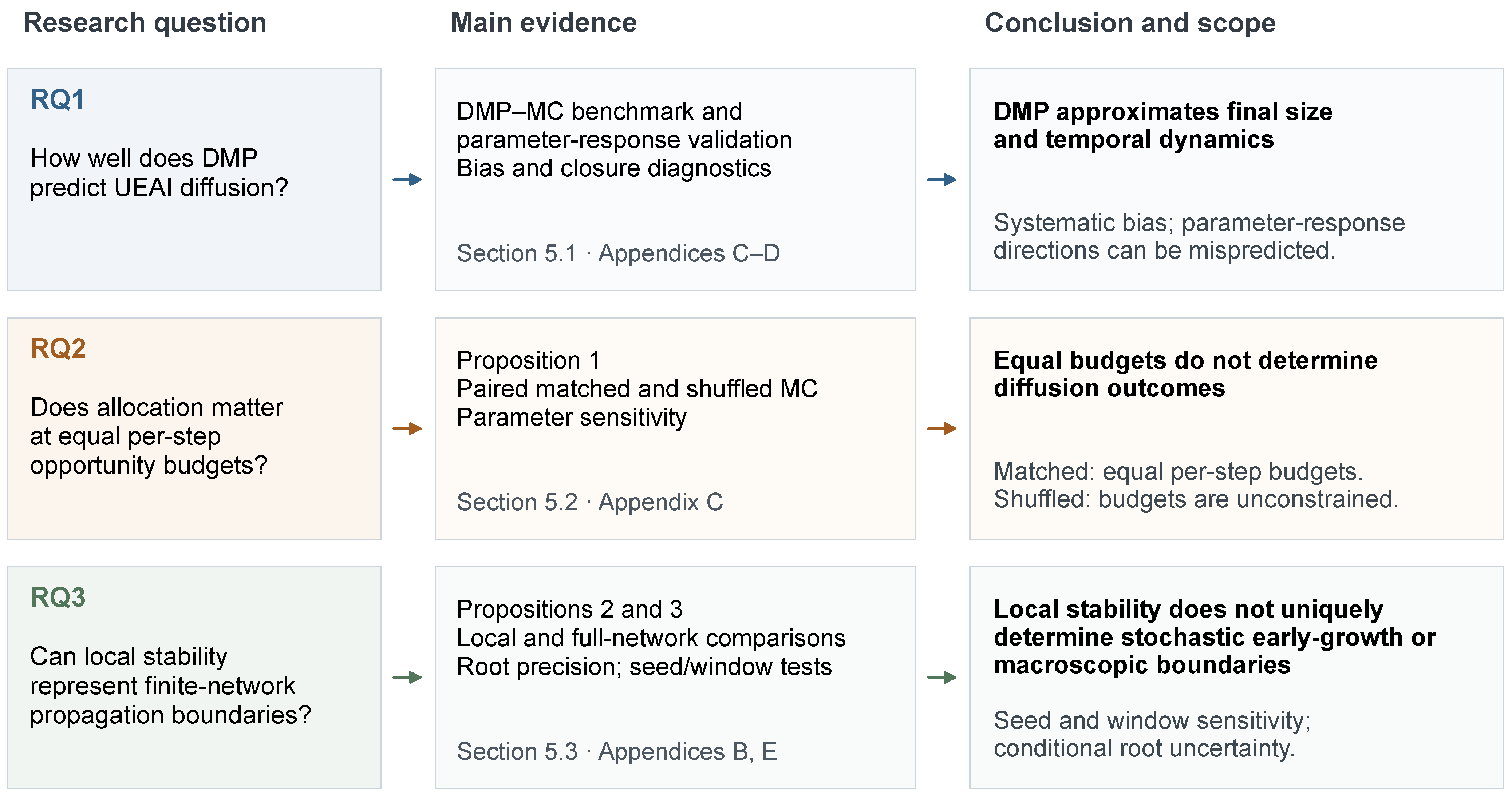
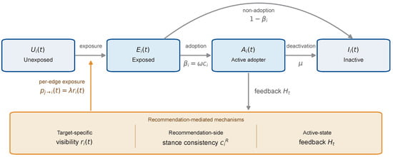
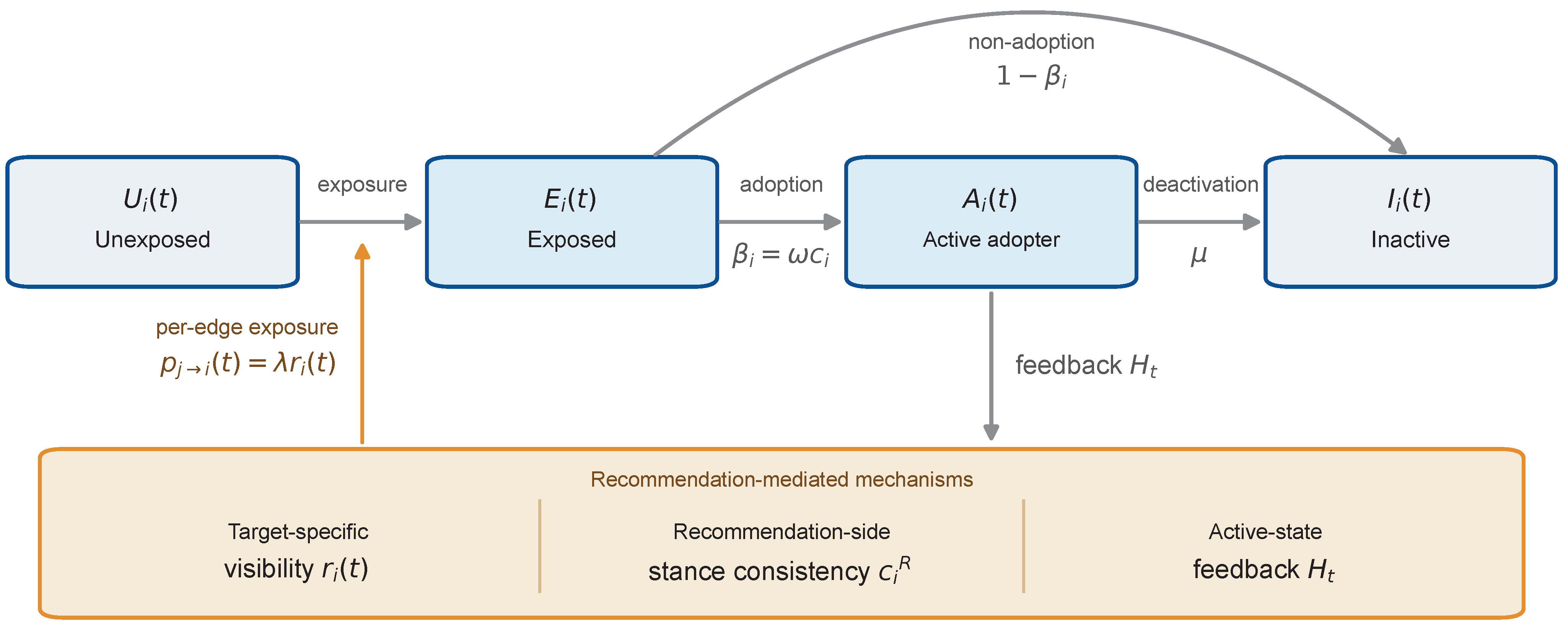
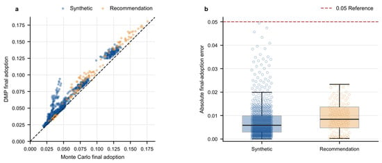
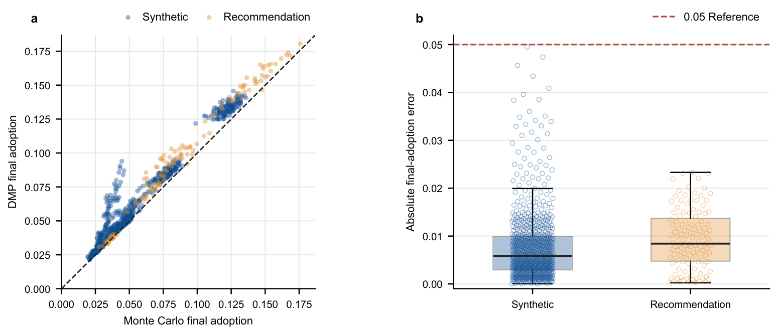
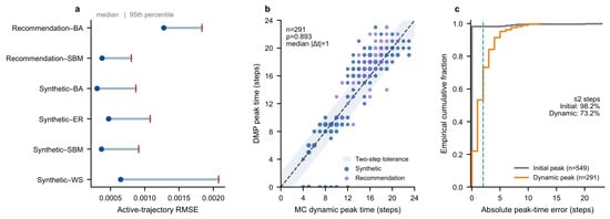
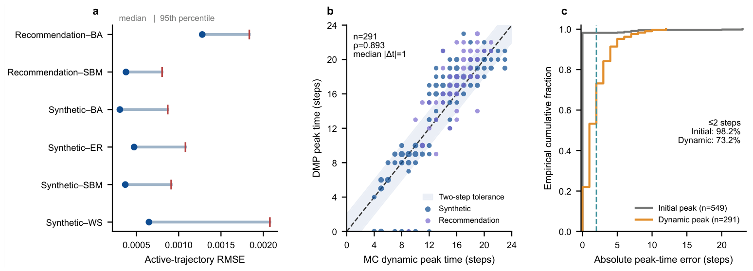
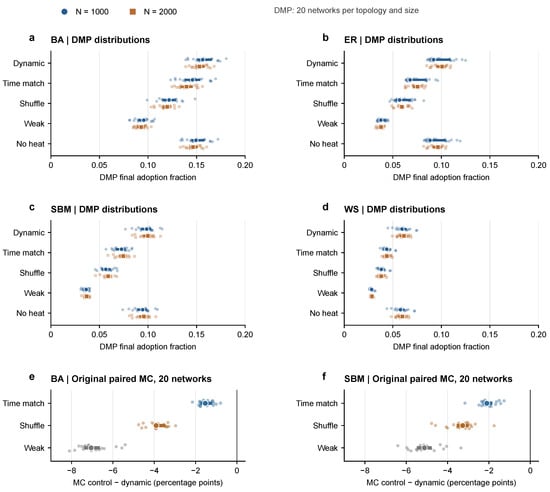
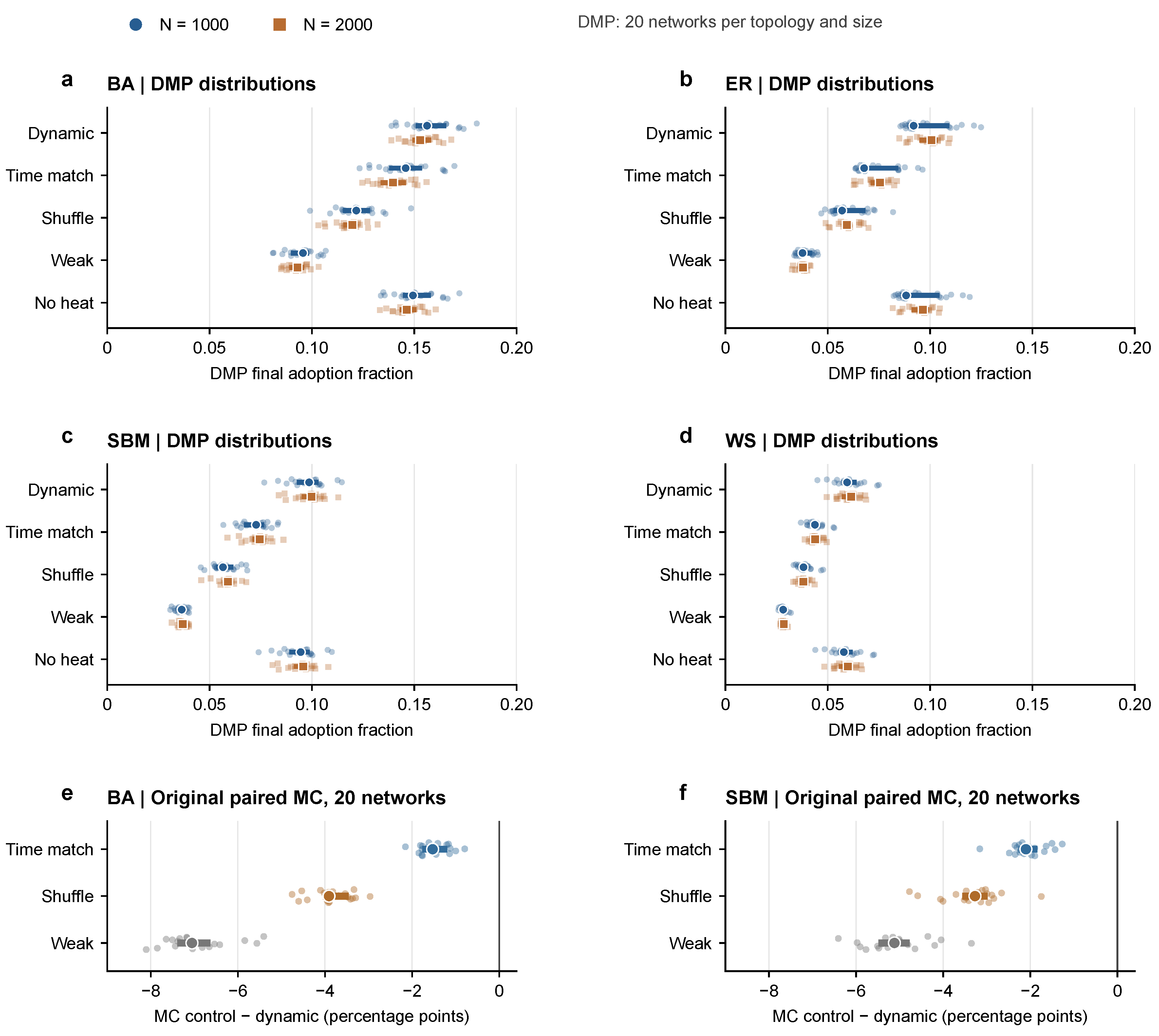
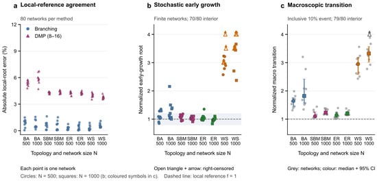
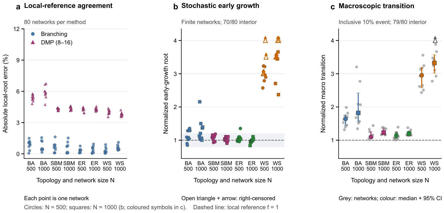

Disclaimer/Publisher’s Note: The statements, opinions and data contained in all publications are solely those of the individual author(s) and contributor(s) and not of MDPI and/or the editor(s). MDPI and/or the editor(s) disclaim responsibility for any injury to people or property resulting from any ideas, methods, instructions or products referred to in the content. |
© 2026 by the authors. Licensee MDPI, Basel, Switzerland. This article is an open access article distributed under the terms and conditions of the Creative Commons Attribution (CC BY) license.