Stability and Error Analysis of Multistep IMEX Local Discontinuous Galerkin Methods for One-Dimensional Nonlinear Fourth-Order Evolution Problems

Abstract

We study three multistep implicit–explicit (IMEX) time discretizations coupled with a local discontinuous Galerkin (LDG) spatial discretization for a class of one-dimensional nonlinear fourth-order partial differential equations (PDEs), with particular emphasis on the Kuramoto–Sivashinsky (KS) equation. The nonlinear convection is treated explicitly, whereas the linear second-, third-, and fourth-derivative terms are advanced implicitly. Under the quasi-uniform mesh assumption and a uniform boundedness assumption on the exact and numerical solutions, energy estimates yield $L^2$ stability for the three schemes under a time-step restriction $\tau \le {\tau }_0$, where ${\tau }_0$ is independent of the spatial mesh size. For all three schemes, a coupled LDG elliptic projection and energy estimates give the optimal spatial rate $O\left(h^{N+1}\right)$ together with temporal rates $O\left(\tau \right)$, $O\left({\tau }^2\right)$, and $O\left({\tau }^3\right)$, provided the multistep starting values have the corresponding accuracy. The error analysis uses a coupled LDG elliptic projection so that the discrete auxiliary error equations remain homogeneous; the residual lower-order projection terms, including the $\beta$-term, are estimated explicitly. An independent periodic manufactured-solution test verifies temporal rates approaching one, two, and three. A separate periodic spatial-refinement test at $T=0.5$ with the third-order formula recovers the expected $O\left(h^{N+1}\right)$ spatial behavior. For a long-time periodic KS test, kinetic-energy histories and spatial spectra are compared under both time-step and mesh refinement. The latter diagnostics are interpreted as robustness checks over a finite observation window rather than as evidence of a statistically stationary chaotic state or pointwise long-time convergence.

1. Introduction

In this paper we investigate three specific multistep IMEX time discretizations coupled with an LDG spatial discretization for the one-dimensional nonlinear fourth-order time-dependent problem

$$\left\{\begin{array}{cc}{u}_t+{\partial }_{x}f\left(u\right)+\alpha u_{xx}+\beta u_{xxx}+\epsilon u_{xxxx}=0,\hfill & (x,t)\in I\times (0,T],\hfill \\ u(x,0)=u_0\left(x\right),\hfill & x\in I,\hfill \end{array}\right.$$

(1)

where $I=(a,b)$ is a bounded interval, $\alpha ,\beta \in \mathbb{R}$, and $\epsilon >0$. Throughout, $f\left(u\right)$ is assumed sufficiently smooth in a neighborhood of the exact solution u. In (1), the fourth-order term $\epsilon u_{xxxx}$ supplies high-frequency dissipation, the second-order term $\alpha u_{xx}$ is destabilizing when $\alpha >0$, and the third-order term $\beta u_{xxx}$ is dispersive. When $f\left(u\right)=\frac{u^2}{2}$, (1) reduces to the generalized Kuramoto–Sivashinsky (GKS) equation, a nonlinear dissipative–dispersive model arising in interfacial flows, flame fronts, and thin-film dynamics, well known for pattern formation and deterministic chaos. The specialization $(\beta =0)$ yields the Kuramoto–Sivashinsky (KS) equation, a canonical nonlinear evolution model that arises in many settings—long waves on thin films, interfacial waves between viscous fluids [1], unstable drift waves in plasmas, reaction–diffusion systems [2], and flame-front instability [3]. In particular, with $(\alpha =\epsilon =1)$ and $(\beta =0)$, the KS equation describes pattern formation on unstable flame fronts and thin hydrodynamic films [4]. Its dynamics stem from a competition between the destabilizing second-order term $\left(u_{xx}\right)$ (negative diffusion) and the stabilizing fourth-order term $\left(u_{xxxx}\right)$ (hyperviscosity), nonlinearly regulated by the Burgers-type convection $u{u}_x$. This interplay produces rich behavior: permanent-form traveling waves, coarsening transients, and ultimately deterministic spatio-temporal chaos on sufficiently long, periodic domains [5,6]. The model is translation-invariant and Galilean-invariant, and it exhibits a natural energy-production/dissipation balance that underlies its pattern-selection mechanisms. Chaotic behavior is especially prevalent when (1) is solved on a finite interval with periodic boundary conditions, where small perturbations amplify, interact, and organize into slanted “stripe” structures before merging into a sustained chaotic regime.

We develop a fully discrete analysis for one-dimensional, nonlinear, time-dependent fourth-order PDEs. To mitigate the stringent time-step restrictions of explicit methods for high-order PDEs, we employ a class of multistep IMEX time discretizations [7], in which the nonlinear convection is advanced explicitly, while all lower-order derivative terms together with the fourth-order term are treated implicitly. For the spatial discretization, we use the LDG method.

The LDG method emerged from the discontinuous Galerkin (DG) framework for hyperbolic conservation laws, where high-order Runge–Kutta DG schemes were first developed [8]. To treat diffusion and higher-order operators while preserving locality, Cockburn and Shu introduced LDG for convection–diffusion equations, using auxiliary variables and alternating numerical traces [9]. This development was inspired by the viscous DG discretizations of Bassi and Rebay for the compressible Navier–Stokes equations [10]. It inherits the hallmark advantages of DG methods—robust stability properties, high-order accuracy, and flexible $hp$-adaptivity on complex geometries—while offering a distinctive benefit: local solvability. In particular, the auxiliary variables introduced to approximate gradients can be eliminated elementwise, yielding compact algebraic structures. Over the past two decades, LDG formulations have been developed and analyzed for a wide range of models in steady, semidiscrete, and fully discrete settings, including convection–diffusion systems [9], elliptic problems [11], KdV-type equations [12], the Stokes equations [13], time-dependent fourth-order equations [14], and Hamilton–Jacobi equations [15], among many others.

For the Kuramoto–Sivashinsky equation specifically, several established alternatives motivate the present fully discrete comparison. Xu and Shu [16] developed LDG discretizations for the KS equation and combined them with explicit Runge–Kutta and exponential time-differencing integrators. Akrivis and Smyrlis [17] analyzed implicit–explicit BDF discretizations of the periodic KS problem with a pseudospectral spatial approximation. Kassam and Trefethen [18] compared a stabilized fourth-order exponential time-differencing method with IMEX, integrating-factor, splitting, and related schemes on several stiff PDEs, including KS. These works show that neither LDG spatial discretization nor IMEX treatment of KS is new by itself; the contribution here is the particular multistep IMEX–LDG coupling and its mesh-independent stability and fully discrete error analysis for the nonlinear fourth-order model considered below.

A careful time discretization is essential to preserve the stability, accuracy, and efficiency of the LDG spatial scheme. The explicit Runge–Kutta (RK) time integrators for LDG have been analyzed in detail [8], and they are well suited for convection-dominated convection–diffusion problems due to their simplicity and strong stability properties. However, when diffusion is not negligible, explicit schemes face a severe time-step restriction for stability [19]. A natural remedy is to adopt implicit marching for the stiff terms. In many applications the convection part is nonlinear, making it attractive to treat convection explicitly while advancing the (typically linear) diffusion terms implicitly—an approach known as IMEX time discretization [20]. Even in the presence of nonlinear diffusion, IMEX formulations retain an elliptic-like algebraic structure for the implicit solve, amenable to efficient iterative methods. By contrast, treating both convection and diffusion implicitly generally yields a more complicated, non-elliptic system for which iterative solvers tend to converge poorly.

Combining single- or multistep IMEX time integration with LDG discretization provides a robust, high-order approach for classical convection–diffusion models [21,22]. A principal advantage of these IMEX formulations is that the admissible time-step can be bounded independently of the spatial mesh size h, avoiding a mesh-dependent CFL restriction. In particular, for one-dimensional linear time-dependent fourth-order PDEs, comprehensive stability analyses and error estimates for LDG methods with IMEX time marching have been developed in [23], establishing unconditional energy stability and optimal convergence rates.

A review of the closely related literature from 2023–2026 shows several developments that are particularly relevant to the present problem. Zhang [24] proposed an energy-based DG method for fourth-order semilinear wave equations, emphasizing energy structure and optimal spatial accuracy. Of direct relevance, Lin et al. [25] studied the KdV–Burgers–Kuramoto equation

$$u_t+u{u}_x+\alpha u_{xx}+\beta u_{xxx}+\gamma u_{xxxx}=0,$$

which coincides with (1) when $f\left(u\right)=u^2/2$ and $\gamma =\epsilon$. They developed an ultra-weak LDG method with generalized numerical fluxes, introduced multi-parameter global projections to handle the several spatial derivatives, and established stability and optimal spatial error estimates. Their analysis is centered on the spatial UWLDG discretization, whereas the present work develops a fully discrete stability and error analysis for three multistep IMEX–LDG couplings applied to the same nonlinear fourth-order model. Li, Meng, and Li [26] analyzed generalized-flux LDG approximations for one-dimensional nonlinear time-dependent fourth-order equations, proving $L^2$ stability and optimal $O\left(h^{k+1}\right)$ spatial accuracy. Their theoretical results are extended to an equation with an additional dispersion term and to mixed boundary conditions; their numerical examples also include Dirichlet and generalized Dirichlet data, singularly perturbed problems, and two-dimensional problems. Li, Meng, and Wu [27] further established superconvergence results for this class of nonlinear fourth-order equations using generalized Gauss–Radau projections and correction functions. At the fully discrete level, Zhou, Chen, and Guo [28] coupled an ultra-weak LDG discretization with spectral deferred correction time marching for a linear fourth-order equation and proved unconditional stability and optimal error estimates for schemes of up to fourth temporal order. This result is close in spirit to the present fully discrete analysis, but it treats a linear model and uses SDC rather than multistep IMEX time integration.

Recent work has also broadened fourth-order discretization in other directions. Fu et al. [29] analyzed UWLDG schemes for linear time-dependent fourth-order problems under several boundary conditions in one and two dimensions, while Fu, Shu, and Tao [30] treated the nonlinear extended Fisher–Kolmogorov equation with UWLDG schemes and derived energy stability and optimal spatial accuracy for non-periodic boundary conditions. Liu and Cheng [31] and Liu, Wang, and Cheng [32] developed LDG schemes on layer-adapted meshes for singularly perturbed fourth-order reaction–diffusion and convection–diffusion boundary-value problems. For the classical KS equation, Doss and Kousalya [33] used a meshfree finite-pointset method after a second-order splitting, whereas Doss and Sindhujarani [34] developed a two-dimensional mixed $H^1$ Galerkin method whose fully discrete formulation uses backward Euler time-stepping. Recent fractional KS studies, such as the quintic B-spline method of Choudhary et al. [35] and the fast compact scheme of Jiang and Xu [36], concern Caputo time derivatives and hence a different temporal model. Aboelenen et al. [37] coupled ALE–LDG spatial discretization on moving meshes with IMEX time discretization, addressing a moving-domain setting rather than the fixed-mesh multistep setting considered here.

From the time-integration viewpoint, high-order IMEX–Runge–Kutta/DG coupling has been studied by Kanevsky et al. [38], and recent IMEX–RK stability and convergence analysis for reaction–diffusion equations was given by Gu et al. [39]. Broader recent high-order analyses for other models include linear and decoupled IMEX schemes for the Ericksen–Leslie model [40], an energy-stable tetrahedral spectral-element discretization for a Kohn–Sham gradient-flow model [41], a compressed-Legendre method for time-fractional convection–diffusion equations [42], and a modified Galerkin method for derivative-dependent Fredholm–Hammerstein equations [43]. These works provide recent numerical-analysis context but address different model equations.

Against this background, the contribution of the present paper is the fully discrete analysis of three multistep IMEX–LDG methods for the one-dimensional nonlinear fourth-order problem (1). The nonlinear convection is treated explicitly, while the linear second-, third-, and fourth-derivative terms are treated implicitly. We prove $L^2$ stability under a step-size condition $\tau \le {\tau }_0$ with ${\tau }_0$ independent of the mesh size h, and derive the fully discrete bounds $O(h^{N+1}+\tau )$, $O(h^{N+1}+{\tau }^2)$, and $O(h^{N+1}+{\tau }^3)$ under the corresponding startup assumptions. Thus the novelty is not LDG discretization of the KS/KBK model itself; in particular, Lin et al. [25] already provide a rigorous UWLDG spatial analysis for the same equation. The distinction is the common fully discrete stability/error framework for three multistep IMEX couplings, including the nonlinear convective perturbation and the simultaneous second-, third-, and fourth-order linear operators.

The remainder of the paper is organized as follows. In Section 2, we describe the finite element spaces, summarize the LDG method, and give the semidiscrete formulation for the nonlinear fourth-order system.

In Section 3, we prove stability of the three multistep IMEX–LDG methods. Section 4 gives optimal fully discrete error estimates for all three schemes. Section 5 presents numerical experiments that illustrate the accuracy and robustness of the schemes. Section 6 offers concluding remarks.

2. The LDG Method

This section develops the semidiscrete LDG formulation of the nonlinear fourth-order problem. Introduce auxiliary variables $R,Q,P$ to factor the fourth derivative into a chain of first derivatives:

$$P={\partial }_{x}Q,Q={\partial }_{x}R,R={\partial }_{x}U.$$

(2)

This first-order system is coupled with the primary equation in the LDG framework to approximate the fourth-order operator via an alternating, energy-stable gradient–divergence pair. Hence, the fourth-order PDE is equivalently written as

$$\begin{array}{cc}\hfill & \frac{\partial U}{\partial t}+\alpha \frac{\partial }{\partial x}R+\beta \frac{\partial }{\partial x}Q+\frac{\partial }{\partial x}f\left(U\right)+\epsilon \frac{\partial }{\partial x}P=0,\hfill \\ \hfill & P=\frac{\partial }{\partial x}Q,Q=\frac{\partial }{\partial x}R,R=\frac{\partial }{\partial x}U.\hfill \end{array}$$

(3)

Let ${\Omega }_h={\left\{D^k\right\}}_{k=1}^K$ be a partition of I with $D^k=[x_{k-\frac{1}{2}},x_{k+\frac{1}{2}}]$ and $h_k=x_{k+\frac{1}{2}}-x_{k-\frac{1}{2}}$, $h={\max }_k{h}_k$. We assume a quasi-uniform family of meshes: there exists a constant $\kappa >0$, independent of h, such that $\kappa h\le h_k\le h$ for every element. For a fixed polynomial degree $N\ge 0$ define

$$V_h^N:=\{v\in L^2\left(I\right):v{|}_{D^k}\in {\mathbb{P}}^N\left(D^k\right),k=1,\dots ,K\},H^r\left({\Omega }_h\right):=\{v\in L^2\left(I\right):v{|}_{D^k}\in H^r\left(D^k\right)\forall k\}.$$

(4)

For brevity, we write $V_h:=V_h^N$ throughout the remainder of the paper. Local and global $L^2$ inner products are

$${(u,v)}_{D^k}:={\int }_{D^k}uvdx,{\parallel u\parallel }_{D^k}^2={(u,u)}_{D^k},(u,v):={\displaystyle \sum _{k=1}^K}{(u,v)}_{D^k}.$$

At each interior interface $x_{k+\frac{1}{2}}$ we use standard traces, jumps, and averages:

$$\begin{array}{cc}\hfill & w^{\pm }\left(x_i\right)=\underset{x\to x_i^{\pm }}{\lim }w\left(x\right),{\left\{\left\{w\right\}\right\}}_{k-\frac{1}{2}}=\frac{1}{2}(w_{k-\frac{1}{2}}^{+}+w_{k-\frac{1}{2}}^{-}),〚w{〛}_{k-\frac{1}{2}}=w_{k-\frac{1}{2}}^{+}-w_{k-\frac{1}{2}}^{-}.\hfill \end{array}$$

(5)

The LDG scheme seeks approximations $u_h,r_h,q_h,p_h\in V_h^N$ such that the following variational forms hold for all $v,\psi ,\varphi ,\phi \in V_h^N$:

$$\begin{array}{cc}\hfill & {\left(\frac{\partial u_h}{\partial t},v\right)}_{D^k}-{\mathcal{N}}_{D^k}(f\left(u_h\right),v)-\alpha {\mathcal{L}}_{D^k}^{+}(r_h,v)-\beta {\mathcal{L}}_{D^k}^{+}(q_h,v)-\epsilon {\mathcal{L}}_{D^k}^{+}(p_h,v)=0,\hfill \\ \hfill & {\left(p_h,\varphi \right)}_{D^k}=-{\mathcal{L}}_{D^k}^{-}(q_h,\varphi ),\hfill \\ \hfill & {\left(q_h,\psi \right)}_{D^k}=-{\mathcal{L}}_{D^k}^{+}(r_h,\psi ),\hfill \\ \hfill & {\left(r_h,\phi \right)}_{D^k}=-{\mathcal{L}}_{D^k}^{-}(u_h,\phi ),\hfill \end{array}$$

(6)

where

$$\begin{array}{cc}\hfill & {\mathcal{N}}_{D^k}(f\left(u\right),w)={(f\left(u\right),\frac{\partial }{\partial x}w)}_{D^k}-\widehat{f}{\left(u\right)}_{k+\frac{1}{2}}{w}_{k+\frac{1}{2}}^{-}+\widehat{f}{\left(u\right)}_{k-\frac{1}{2}}{w}_{k-\frac{1}{2}}^{+},\hfill \\ \hfill & {\mathcal{L}}_{D^k}^{\pm }(r,w)={(r,\frac{\partial }{\partial x}w)}_{D^k}-r_{k+\frac{1}{2}}^{\pm }{w}_{k+\frac{1}{2}}^{-}+r_{k-\frac{1}{2}}^{\pm }{w}_{k-\frac{1}{2}}^{+}.\hfill \end{array}$$

(7)

Summing the elemental formulations (6) over $k=1,\dots ,K$ yields

$$\begin{array}{cc}\hfill & {\displaystyle \sum _{k=1}^K}{(\frac{\partial u_h}{\partial t},v)}_{D^k}-{\displaystyle \sum _{k=1}^K}{\mathcal{N}}_{D^k}(f\left(u_h\right),v)-\alpha {\displaystyle \sum _{k=1}^K}{\mathcal{L}}_{D^k}^{+}(r_h,v)-\beta {\displaystyle \sum _{k=1}^K}{\mathcal{L}}_{D^k}^{+}(q_h,v)-\epsilon {\displaystyle \sum _{k=1}^K}{\mathcal{L}}_{D^k}^{+}(p_h,v)=0,\hfill \\ \hfill & {\displaystyle \sum _{k=1}^K}{\left(p_h,\varphi \right)}_{D^k}=-{\displaystyle \sum _{k=1}^K}{\mathcal{L}}_{D^k}^{-}(q_h,\varphi ),\hfill \\ \hfill & {\displaystyle \sum _{k=1}^K}{\left(q_h,\psi \right)}_{D^k}=-{\displaystyle \sum _{k=1}^K}{\mathcal{L}}_{D^k}^{+}(r_h,\psi ),\hfill \\ \hfill & {\displaystyle \sum _{k=1}^K}{\left(r_h,\phi \right)}_{D^k}=-{\displaystyle \sum _{k=1}^K}{\mathcal{L}}_{D^k}^{-}(u_h,\phi ).\hfill \end{array}$$

(8)

For compactness, define the global inner product and operators

$$\begin{array}{cc}\hfill & \left(r,w\right)={\displaystyle \sum _{k=1}^K}{\left(r,w\right)}_{D^k},\mathcal{N}={\displaystyle \sum _{k=1}^K}{\mathcal{N}}_{D^k},{\mathcal{L}}^{\pm }={\displaystyle \sum _{k=1}^K}{\mathcal{L}}_{D^k}^{\pm }.\hfill \end{array}$$

(9)

With boundary conditions taken into account, the global variational formulation reads: find $u_h,r_h,q_h,p_h\in V_h$ such that, for all $v,\varphi ,\psi ,\phi \in V_h$,

$$\begin{array}{cc}\hfill & (\frac{\partial u_h}{\partial t},v)-\mathcal{N}(f\left(u_h\right),v)-\alpha {\mathcal{L}}^{+}(r_h,v)-\beta {\mathcal{L}}^{+}(q_h,v)-\epsilon {\mathcal{L}}^{+}(p_h,v)=0,\hfill \end{array}$$

(10a)

$$\begin{array}{cc}\hfill & \left(p_h,\varphi \right)=-{\mathcal{L}}^{-}(q_h,\varphi ),\hfill \end{array}$$

(10b)

$$\begin{array}{cc}\hfill & \left(q_h,\psi \right)=-{\mathcal{L}}^{+}(r_h,\psi ),\hfill \end{array}$$

(10c)

$$\begin{array}{cc}\hfill & \left(r_h,\phi \right)=-{\mathcal{L}}^{-}(u_h,\phi ).\hfill \end{array}$$

(10d)

The stability and error analyses below are stated for periodic boundary conditions, for which the alternating LDG interface contributions telescope exactly. For nonhomogeneous Dirichlet data, the corresponding summation-by-parts calculation contains additional physical-boundary flux terms, so the periodic energy identities used below do not hold verbatim. Extending the theorems to that setting would require a boundary lifting and a separate control of those boundary contributions, which is outside the present analysis. Accordingly, the traveling-wave tests with nonhomogeneous Dirichlet data are used only as numerical illustrations and are not presented as verification of the periodic energy theorem. To verify the temporal and spatial convergence behavior within the precise setting of the analysis, Section 5 includes separate smooth manufactured-solution tests with periodic boundary conditions.

Lemma 1 

(LDG adjoint identity). For $a,b\in V_h$, the alternating LDG operators satisfy

$${\mathcal{L}}^{+}(a,b)+{\mathcal{L}}^{-}(b,a)=0.$$

Proof. 

Sum the two elemental forms defined in (7) over the mesh and integrate the volume terms by parts elementwise. At every interior interface, the trace chosen by ${\mathcal{L}}^{+}$ is paired with the opposite trace chosen by ${\mathcal{L}}^{-}$. The resulting interface contributions cancel pairwise. The two physical-boundary contributions cancel as well under periodic boundary conditions, which gives the stated identity. □

Corollary 1 

(Basic LDG energy identities). Let $(u_h,r_h,q_h,p_h)$ satisfy (10b–d). Then

$$\begin{array}{cc}\hfill {\mathcal{L}}^{+}(r_h,u_h)& ={\parallel r_h\parallel }^2,\hfill \end{array}$$

(11)

$$\begin{array}{cc}\hfill {\mathcal{L}}^{+}(q_h,u_h)& =(r_h,q_h),\hfill \end{array}$$

(12)

$$\begin{array}{cc}\hfill {\mathcal{L}}^{+}(p_h,u_h)& =-{\parallel q_h\parallel }^2,\hfill \end{array}$$

(13)

$$\begin{array}{cc}\hfill {\parallel r_h\parallel }^2& =-(q_h,u_h)\le \parallel q_h\parallel \parallel u_h\parallel .\hfill \end{array}$$

(14)

Proof. 

Apply Lemma 1 to the auxiliary relations. Taking $\phi =r_h$ in (10d) gives ${\parallel r_h\parallel }^2=-{\mathcal{L}}^{-}(u_h,r_h)={\mathcal{L}}^{+}(r_h,u_h)$. Taking $\phi =q_h$ in (10d) gives $(r_h,q_h)={\mathcal{L}}^{+}(q_h,u_h)$. Next, taking $\psi =q_h$ in (10c) and $\varphi =r_h$ in (10b) yields $(p_h,r_h)=-{\parallel q_h\parallel }^2$. Finally, Lemma 1 and (10d) with $\phi =p_h$ give ${\mathcal{L}}^{+}(p_h,u_h)=(p_h,r_h)=-{\parallel q_h\parallel }^2$. The last relation follows from (10c,d) and Cauchy–Schwarz. □

Lemma 2 

(Non-positivity of the convective form). Assume that $\widehat{f}$ is a consistent monotone numerical flux. Then, for every $v\in V_h$,

$$\mathcal{N}\left(f\right(v),v)\le 0.$$

Proof. 

This is the standard scalar cell-entropy inequality for a consistent monotone numerical flux. Indeed, after integrating $(f\left(v\right),v_x)$ elementwise, the volume terms reduce to interface entropy-flux differences, while consistency and monotonicity of $\widehat{f}$ make the remaining interface contribution non-positive; see Jiang and Shu [44]. Periodicity removes the two physical-boundary terms. □

Lemma 3 

(Inverse and trace inequalities). There exists a constant $\mu >0$, independent of h, such that for every $v\in V_h$ and every element $D^k$,

$${\parallel v_x\parallel }_{D^k}\le \mu h_k^{-1}{\parallel v\parallel }_{D^k},{\parallel v\parallel }_{\partial D^k}\le \sqrt{\mu h_k^{-1}}{\parallel v\parallel }_{D^k}.$$

(15)

These are the standard finite element inverse and trace estimates on a quasi-uniform one-dimensional mesh; see, for example, [9,21].

Lemma 4 

(Discrete derivative control). Let $w,r,q\in V_h$ satisfy the two consecutive LDG relations

$$(r,\phi )=-{\mathcal{L}}^{-}(w,\phi ),(q,\psi )=-{\mathcal{L}}^{+}(r,\psi )$$

for all test functions. Then there exists a mesh-independent constant $C_{\mu }>0$ such that

$$\parallel w_x\parallel +\sqrt{\mu h^{-1}}\left|\left[w\right]\right|\le C_{\mu }\parallel r\parallel ,\parallel r_x\parallel +\sqrt{\mu h^{-1}}\left|\left[r\right]\right|\le C_{\mu }\parallel q\parallel .$$

(16)

Here $\left|\right[·\left]\right|$ denotes the global interface-jump seminorm. This is the standard LDG inverse/trace estimate; see, for example, Lemma 2.5 of [23].

Lemma 5 

(Discrete Poincaré inequality). If $v\in V_h$ is periodic and has zero mean, then

$$\parallel v\parallel \le C_P\left(\parallel v_x\parallel +h^{-1/2}\left|\left[v\right]\right|\right),$$

(17)

where $C_P$ is independent of h.

Proof. 

This is the broken one-dimensional Poincaré inequality. Apply the continuous Poincaré estimate on each element after subtracting its cell average; differences of neighboring cell averages are controlled by the interface jumps. Summing over the periodic mesh and using the zero-mean condition gives (17), with a constant independent of h on a quasi-uniform family. □

Corollary 2 

(Control of the first LDG derivative). Under periodic boundary conditions, any LDG state satisfying the two auxiliary relations in Lemma 4 has a first derivative variable r with zero mean. Consequently, Lemmas 4 and 5 imply

$$\parallel r\parallel \le C_P{C}_{\mu }\parallel q\parallel .$$

(18)

The same estimate holds for differences of two LDG states and, in Section 4, for the discrete errors generated by the coupled LDG elliptic projection.

Proof. 

Set the test function equal to the constant 1 in the LDG relation defining r. The volume derivative vanishes, and the alternating numerical traces telescope around the periodic mesh; hence $(r,1)=0$. Applying Lemma 5 to r and then the second estimate in Lemma 4 gives

$$\parallel r\parallel \le C_P\left(\parallel r_x\parallel +h^{-1/2}\left|\left[r\right]\right|\right)\le C_P{C}_{\mu }\parallel q\parallel .$$

The argument is linear and therefore applies unchanged to differences of two LDG states and to projected error variables. □

We make the following uniform bounded-range assumption for the nonlinear convection. There exists $M>0$, independent of h and $\tau$, such that all exact and numerical states entering the stability and error estimates satisfy

$${\parallel U(·,t)\parallel }_{L^{\infty }\left(I\right)}\le M,{\parallel u^n\parallel }_{L^{\infty }\left(I\right)}\le M,0\le t\le T.$$

(19)

The bound (19) is an explicit hypothesis of the present nonlinear analysis; we do not claim to derive an h-independent discrete $L^{\infty }$ bound from the energy estimate alone. A direct use of one-dimensional inverse inequalities would introduce negative powers of h and therefore does not, by itself, close the mesh-independent estimate required below. A standard alternative is to replace f by a smooth cut-off $f_M$ that agrees with the physical flux on $[-M,M]$ and has a globally bounded derivative. The proof then applies without an a priori $L^{\infty }$ assumption to the cut-off problem; whenever the computed and exact states remain in $[-M,M]$, the cut-off and original schemes coincide. Thus the role of (19) is precisely to keep the nonlinear Lipschitz constants independent of h and $\tau$. In particular, assume that f is differentiable on $[-M,M]$ and that the numerical flux is Lipschitz there: for some $C_f=C_f\left(M\right)>0$ independent of h and $\tau$,

$$\left|f^{\prime }\left(w\right)\right|\le C_f\left(\right|w|\le M),|\widehat{f}(a,c)-\widehat{f}(b,d)|\le C_f\left(\right|a-b|+|c-d\left|\right)\left(\right|a|,|b|,|c|,|d|\le M).$$

(20)

For $a,b,v\in V_h$ define

$$\mathcal{D}(a,b;v):=\mathcal{N}\left(f\right(a),v)-\mathcal{N}\left(f\right(b),v).$$

Lemma 6 

(Lipschitz estimate for convection). Assume (20). Let a be a bounded piecewise $H^1$ function with well-defined traces, let $b,\chi ,v\in V_h$, and write $a-b=(\chi -b)-(\chi -a)$. Then

$$\begin{array}{cc}\hfill \left|\mathcal{D}\right(a,b;v\left)\right|& \le C_f\left(\parallel \chi -b\parallel +\parallel a-\chi \parallel +h^{1/2}{\parallel a-\chi \parallel }_{\partial {\Omega }_h}\right)\hfill \\ \hfill & \times \left(\parallel v_x\parallel +\sqrt{\mu h^{-1}}\left|\left[v\right]\right|\right).\hfill \end{array}$$

(21)

If v is paired with homogeneous LDG auxiliary variables $(r_v,q_v)$, Lemma 4 and Corollary 2 imply

$$\left|\mathcal{D}(a,b;v)\right|\le C\left(\parallel \chi -b\parallel +\parallel a-\chi \parallel +h^{1/2}{\parallel a-\chi \parallel }_{\partial {\Omega }_h}\right)\parallel q_v\parallel .$$

(22)

Proof. 

Subtract the two DG convection forms element by element. The mean-value theorem bounds the volume-flux difference by $C_f|a-b|$. At interfaces, the Lipschitz numerical flux produces traces of $a-b$. Split $a-b=(\chi -b)-(\chi -a)$: the discrete part $\chi -b$ is controlled by the inverse trace inequality, whereas the smooth/projection part $a-\chi$ is retained in the mesh-boundary norm. Cauchy–Schwarz yields (21). For a homogeneous LDG error state, Lemma 4 and Corollary 2 convert the derivative/jump factor into $C\parallel q_v\parallel$, giving (22). This form is valid when a is the exact solution and avoids applying a discrete inverse inequality directly to a. □

Lemma 7 

(Control of the lower-order implicit terms). Let $(u^m,r^m,q^m)$ satisfy the LDG relations at the indicated time levels. For every $\delta >0$ there is a constant $C_{\delta }$, independent of h and τ, such that

$$\left|\alpha \right||(r^i,r^j)|+|\beta ||(r^i,q^j)|\le \delta ({\parallel q^i\parallel }^2+{\parallel q^j\parallel }^2)+C_{\delta }({\parallel u^i\parallel }^2+{\parallel u^j\parallel }^2).$$

(23)

Proof. 

From (14), ${\parallel r^m\parallel }^2\le \parallel q^m\parallel \parallel u^m\parallel$. Apply Cauchy–Schwarz and Young’s inequality to $(r^i,r^j)$ and $(r^i,q^j)$, and then use (14) at the required time levels. The resulting constants may depend on $\left|\alpha \right|$, $\left|\beta \right|$, $\epsilon$, and $\delta$, but not on h or $\tau$. □

3. Multistep IMEX–LDG Time Discretization Schemes

Let $\tau >0$ be uniform and $t^n=n\tau$. At every stored time level the LDG auxiliary variables are defined by

$$(p^m,\varphi )=-{\mathcal{L}}^{-}(q^m,\varphi ),(q^m,\psi )=-{\mathcal{L}}^{+}(r^m,\psi ),(r^m,\phi )=-{\mathcal{L}}^{-}(u^m,\phi ).$$

(24)

• First-Order IMEX–LDG Scheme

For $n\ge 0$, given $u^n$, find $(u^{n+1},r^{n+1},q^{n+1},p^{n+1})\in V_h^4$ such that

$$\begin{array}{cc}\hfill (u^{n+1},v)& =(u^n,v)+\tau \mathcal{N}(f\left(u^n\right),v)+\alpha \tau {\mathcal{L}}^{+}(r^{n+1},v)+\beta \tau {\mathcal{L}}^{+}(q^{n+1},v)+\epsilon \tau {\mathcal{L}}^{+}(p^{n+1},v),\hfill \end{array}$$

(25a)

$$\begin{array}{cc}\hfill (p^{n+1},\varphi )& =-{\mathcal{L}}^{-}(q^{n+1},\varphi ),\hfill \end{array}$$

(25b)

$$\begin{array}{cc}\hfill (q^{n+1},\psi )& =-{\mathcal{L}}^{+}(r^{n+1},\psi ),\hfill \end{array}$$

(25c)

$$\begin{array}{cc}\hfill (r^{n+1},\phi )& =-{\mathcal{L}}^{-}(u^{n+1},\phi ).\hfill \end{array}$$

(25d)

• Second-Order IMEX–LDG Scheme

For $n\ge 1$, given the required history, find the new solution from

$$\begin{array}{cc}\hfill (u^{n+1},v)& =(u^n,v)+\tau \left[\frac{3}{2}\mathcal{N}(f\left(u^n\right),v)-\frac{1}{2}\mathcal{N}(f\left(u^{n-1}\right),v)\right]\hfill \\ \hfill & +\alpha \tau \left[\frac{3}{4}{\mathcal{L}}^{+}(r^{n+1},v)+\frac{1}{4}{\mathcal{L}}^{+}(r^{n-1},v)\right]\hfill \\ \hfill & +\beta \tau \left[\frac{3}{4}{\mathcal{L}}^{+}(q^{n+1},v)+\frac{1}{4}{\mathcal{L}}^{+}(q^{n-1},v)\right]\hfill \\ \hfill & +\epsilon \tau \left[\frac{3}{4}{\mathcal{L}}^{+}(p^{n+1},v)+\frac{1}{4}{\mathcal{L}}^{+}(p^{n-1},v)\right].\hfill \end{array}$$

(26)

together with (24) at the required time levels. For the stability theorem below, the starting history is treated as given. For the second-order error estimate, the starting values are required to satisfy the explicit consistency condition (55); no stronger claim about a particular startup procedure is used in the proof.

• Third-Order IMEX–LDG Scheme

The third-order formula uses the Adams–Bashforth three-step extrapolation for convection and the third-order quadrature weights $2/3$, $5/12$, and $-1/12$ at the implicit time levels $t^{n+1}$, $t^{n-1}$, and $t^{n-3}$, respectively. Thus, for $n\ge 3$,

$$\begin{array}{cc}\hfill (u^{n+1},v)& =(u^n,v)+\tau \left[\frac{23}{12}\mathcal{N}(f\left(u^n\right),v)-\frac{4}{3}\mathcal{N}(f\left(u^{n-1}\right),v)+\frac{5}{12}\mathcal{N}(f\left(u^{n-2}\right),v)\right]\hfill \\ \hfill & +\alpha \tau \left[\frac{2}{3}{\mathcal{L}}^{+}(r^{n+1},v)+\frac{5}{12}{\mathcal{L}}^{+}(r^{n-1},v)-\frac{1}{12}{\mathcal{L}}^{+}(r^{n-3},v)\right]\hfill \\ \hfill & +\beta \tau \left[\frac{2}{3}{\mathcal{L}}^{+}(q^{n+1},v)+\frac{5}{12}{\mathcal{L}}^{+}(q^{n-1},v)-\frac{1}{12}{\mathcal{L}}^{+}(q^{n-3},v)\right]\hfill \\ \hfill & +\epsilon \tau \left[\frac{2}{3}{\mathcal{L}}^{+}(p^{n+1},v)+\frac{5}{12}{\mathcal{L}}^{+}(p^{n-1},v)-\frac{1}{12}{\mathcal{L}}^{+}(p^{n-3},v)\right].\hfill \end{array}$$

(27)

together with (24) at all required history levels. The starting values $u^1,u^2,u^3$ must be generated with sufficient accuracy for the intended application. In particular, a third-order temporal convergence study requires starting values with $O\left({\tau }^3\right)$ global accuracy.

Stability Analysis

The constants below may depend on T, $\left|\alpha \right|$, $\left|\beta \right|$, $\epsilon$, the uniform bound M in (19), and the associated flux Lipschitz constant $C_f\left(M\right)$, but are independent of h and $\tau$.

Theorem 1 

(First-order stability). There exist ${\tau }_0>0$, $c_1>0$, and $C_T>0$, with ${\tau }_0$ independent of h, such that the solution of (25) satisfies, for $\tau \le {\tau }_0$,

$${\parallel u^{n+1}\parallel }^2+c_1\epsilon \tau {\displaystyle \sum _{j=0}^n}{\parallel q^{j+1}\parallel }^2\le C_T{\parallel u^0\parallel }^2.$$

(28)

Proof. 

Take $v=u^{n+1}$ in (25a) and use

$$2(u^{n+1}-u^n,u^{n+1})=\parallel u^{n+1}{\parallel }^2-\parallel u^n{\parallel }^2+{\parallel u^{n+1}-u^n\parallel }^2.$$

The convective term is decomposed as

$$\mathcal{N}(f\left(u^n\right),u^{n+1})=\mathcal{N}(f\left(u^{n+1}\right),u^{n+1})-\mathcal{D}(u^{n+1},u^n;u^{n+1}).$$

Lemma 2 makes the first term non-positive. Lemma 6, Corollary 2, and Young’s inequality give

$$\tau |\mathcal{D}(u^{n+1},u^n;u^{n+1})|\le \frac{1}{8}{\parallel u^{n+1}-u^n\parallel }^2+C{\tau }^2{\parallel q^{n+1}\parallel }^2.$$

Using (11)–(13) and Lemma 7, the implicit lower-order terms satisfy, for a sufficiently small fixed $\delta >0$,

$$\tau \left|\alpha \parallel r^{n+1}{\parallel }^2+\beta (r^{n+1},q^{n+1})\right|\le \frac{\epsilon \tau }{4}{\parallel q^{n+1}\parallel }^2+C\tau {\parallel u^{n+1}\parallel }^2,$$

whereas the fourth-order term contributes $-\epsilon \tau {\parallel q^{n+1}\parallel }^2$. We first reduce ${\tau }_0$, if necessary, so that the current-level term $C\tau {\parallel u^{n+1}\parallel }^2$ can be transferred to the left-hand side. We then choose ${\tau }_0$ small enough that the $C{\tau }^2{\parallel q^{n+1}\parallel }^2$ term is absorbed by the fourth-order dissipation. Summing in n and applying discrete Gronwall proves (28). □

Theorem 2 

(Second-order stability). There exist ${\tau }_0>0$, $c_2>0$, and $C_T>0$, independent of h, such that for $\tau \le {\tau }_0$ the solution of (26) satisfies

$${\parallel u^{n+1}\parallel }^2+c_2\epsilon \tau {\displaystyle \sum _{j=1}^n}{\parallel q^{j+1}\parallel }^2\le C_T{\displaystyle \sum _{j=0}^1}\left(\parallel u^j{\parallel }^2+\tau {\parallel q^j\parallel }^2\right).$$

(29)

Proof. 

Set $v=u^{n+1}$ in (26) and write $\Delta u^j:=u^j-u^{j-1}$. The Adams–Bashforth part has the exact decomposition

$$\begin{array}{cc}\hfill & \frac{3}{2}\mathcal{N}(f\left(u^n\right),u^{n+1})-\frac{1}{2}\mathcal{N}(f\left(u^{n-1}\right),u^{n+1})\hfill \\ \hfill & =\mathcal{N}(f\left(u^{n+1}\right),u^{n+1})-\mathcal{D}(u^{n+1},u^n;u^{n+1})+\frac{1}{2}\mathcal{D}(u^n,u^{n-1};u^{n+1}).\hfill \end{array}$$

(30)

The first term is non-positive by Lemma 2. By Lemma 6, Corollary 2, and Young’s inequality, for every fixed $\eta >0$,

$$\begin{array}{cc}\hfill \tau \left|\mathcal{D}\right(u^{n+1},u^n;u^{n+1}\left)\right|& \le \eta \parallel \Delta u^{n+1}{\parallel }^2+C_{\eta }{\tau }^2{\parallel q^{n+1}\parallel }^2,\hfill \end{array}$$

(31)

$$\begin{array}{cc}\hfill \frac{\tau }{2}\left|\mathcal{D}(u^n,u^{n-1};u^{n+1})\right|& \le \eta \parallel \Delta u^n{\parallel }^2+C_{\eta }{\tau }^2{\parallel q^{n+1}\parallel }^2.\hfill \end{array}$$

(32)

Using the identity

$$2(\Delta u^{n+1},u^{n+1})=\parallel u^{n+1}{\parallel }^2-\parallel u^n{\parallel }^2+{\parallel \Delta u^{n+1}\parallel }^2,$$

together with the LDG identities, the fourth-order contribution is

$$-\epsilon \tau \left(\frac{3}{4}{\parallel q^{n+1}\parallel }^2+\frac{1}{4}(q^{n+1},q^{n-1})\right).$$

The history product satisfies

$$-\frac{1}{4}(q^{n+1},q^{n-1})\le \frac{1}{8}{\parallel q^{n+1}\parallel }^2+\frac{1}{8}{\parallel q^{n-1}\parallel }^2.$$

(33)

Furthermore, Lemma 7, applied to all $\alpha$- and $\beta$-terms, gives for arbitrary $\delta >0$

$$\begin{array}{cc}\hfill & \tau \left|\frac{3}{4}\alpha (r^{n+1},r^{n+1})+\frac{1}{4}\alpha (r^{n+1},r^{n-1})+\frac{3}{4}\beta (r^{n+1},q^{n+1})+\frac{1}{4}\beta (r^{n+1},q^{n-1})\right|\hfill \\ \hfill & \le \delta \tau \left(\parallel q^{n+1}{\parallel }^2+{\parallel q^{n-1}\parallel }^2\right)+C_{\delta }\tau \left(\parallel u^{n+1}{\parallel }^2+{\parallel u^{n-1}\parallel }^2\right).\hfill \end{array}$$

(34)

Combining (30)–(34), summing from $j=1$ to n, and shifting the history indices produces a current-level contribution $C\tau \parallel u^{n+1}{\parallel }^2$. By reducing ${\tau }_0$ if necessary, this term is transferred to the left-hand side, and the remaining history terms yield

$$\begin{array}{cc}\hfill & {\parallel u^{n+1}\parallel }^2+c{\displaystyle \sum _{j=1}^n}\parallel \Delta u^{j+1}{\parallel }^2+c\epsilon \tau {\displaystyle \sum _{j=1}^n}{\parallel q^{j+1}\parallel }^2\hfill \\ \hfill & \le C\left(\parallel u^0{\parallel }^2+\parallel u^1{\parallel }^2+\tau \parallel q^0{\parallel }^2+\tau {\parallel q^1\parallel }^2\right)+C\tau {\displaystyle \sum _{j=1}^n}{\parallel u^j\parallel }^2+C{\tau }^2{\displaystyle \sum _{j=1}^n}{\parallel q^{j+1}\parallel }^2.\hfill \end{array}$$

(35)

Here $c>0$ is independent of h and $\tau$: choose first $\eta$ and $\delta$ sufficiently small so that the increment and q-terms are absorbed, and then choose ${\tau }_0$ so that the last term in (35) is absorbed by the fourth-order dissipation for $\tau \le {\tau }_0$. A discrete Gronwall inequality proves (29). □

Theorem 3 

(Third-order stability). There exist ${\tau }_0>0$, $c_3>0$, and $C_T>0$, independent of h, such that for $\tau \le {\tau }_0$ the solution of the third-order scheme (27) satisfies

$${\parallel u^{n+1}\parallel }^2+c_3\epsilon \tau {\displaystyle \sum _{j=3}^n}{\parallel q^{j+1}\parallel }^2\le C_T{\displaystyle \sum _{j=0}^3}\left({\parallel u^j\parallel }^2+\tau {\parallel q^j\parallel }^2\right),n\ge 3.$$

(36)

Proof. 

Take $v=u^{n+1}$ in (27) and again write $\Delta u^j=u^j-u^{j-1}$. The Adams–Bashforth combination admits the exact representation

$$\begin{array}{cc}\hfill & \frac{23}{12}\mathcal{N}(f\left(u^n\right),u^{n+1})-\frac{4}{3}\mathcal{N}(f\left(u^{n-1}\right),u^{n+1})+\frac{5}{12}\mathcal{N}(f\left(u^{n-2}\right),u^{n+1})\hfill \\ \hfill & =\mathcal{N}(f\left(u^{n+1}\right),u^{n+1})-\mathcal{D}(u^{n+1},u^n;u^{n+1})+\frac{11}{12}\mathcal{D}(u^n,u^{n-1};u^{n+1})\hfill \\ \hfill & -\frac{5}{12}\mathcal{D}(u^{n-1},u^{n-2};u^{n+1}).\hfill \end{array}$$

(37)

The first term is non-positive. Lemma 6 and Corollary 2 imply, for every fixed $\eta >0$,

$$\begin{array}{cc}\hfill & \tau \left|-\mathcal{D}(u^{n+1},u^n;u^{n+1})+\frac{11}{12}\mathcal{D}(u^n,u^{n-1};u^{n+1})-\frac{5}{12}\mathcal{D}(u^{n-1},u^{n-2};u^{n+1})\right|\hfill \\ \hfill & \le \eta \left(\parallel \Delta u^{n+1}{\parallel }^2+\parallel \Delta u^n{\parallel }^2+{\parallel \Delta u^{n-1}\parallel }^2\right)+C_{\eta }{\tau }^2{\parallel q^{n+1}\parallel }^2.\hfill \end{array}$$

(38)

For the fourth-order term define

$$B_j:=\frac{2}{3}{\parallel q^{j+1}\parallel }^2+\frac{5}{12}(q^{j+1},q^{j-1})-\frac{1}{12}(q^{j+1},q^{j-3}).$$

By Young’s inequality,

$$B_j\ge \frac{5}{12}{\parallel q^{j+1}\parallel }^2-\frac{5}{24}{\parallel q^{j-1}\parallel }^2-\frac{1}{24}{\parallel q^{j-3}\parallel }^2.$$

(39)

Hence, after summing and shifting the history indices,

$${\displaystyle \sum _{j=3}^n}{B}_j\ge \frac{1}{6}{\displaystyle \sum _{j=3}^n}{\parallel q^{j+1}\parallel }^2-C{\displaystyle \sum _{m=0}^3}{\parallel q^m\parallel }^2,$$

(40)

with an absolute constant C. The lower-order implicit terms are handled by Lemma 7; for every $\delta >0$ their total contribution over $j=3,\dots ,n$ is bounded by

$$\begin{array}{c}\hfill \delta \tau {\displaystyle \sum _{j=3}^n}{\parallel q^{j+1}\parallel }^2+C\delta \tau {\displaystyle \sum _{m=0}^3}{\parallel q^m\parallel }^2+C_{\delta }\tau {\displaystyle \sum _{j=0}^{n+1}}{\parallel u^j\parallel }^2.\end{array}$$

(41)

Combining (37)–(41) with the discrete energy identity produces, in particular, a current-level term $C\tau \parallel u^{n+1}{\parallel }^2$. We reduce ${\tau }_0$ if necessary and transfer this term to the left-hand side; the remaining history terms give

$$\begin{array}{cc}\hfill & {\parallel u^{n+1}\parallel }^2+c{\displaystyle \sum _{j=3}^n}\parallel \Delta u^{j+1}{\parallel }^2+c\epsilon \tau {\displaystyle \sum _{j=3}^n}{\parallel q^{j+1}\parallel }^2\hfill \\ \hfill & \le C{\displaystyle \sum _{m=0}^3}\left(\parallel u^m{\parallel }^2+\tau {\parallel q^m\parallel }^2\right)+C\tau {\displaystyle \sum _{j=3}^n}{\parallel u^j\parallel }^2+C{\tau }^2{\displaystyle \sum _{j=3}^n}{\parallel q^{j+1}\parallel }^2.\hfill \end{array}$$

(42)

Choose $\eta$ and $\delta$ first so that the increment terms and a fixed portion of the dissipation in (40) remain on the left. Then choose ${\tau }_0$ so that the last term in (42) is absorbed whenever $\tau \le {\tau }_0$. Discrete Gronwall yields (36). □

4. Optimal Error Estimates

The error analysis is based on a coupled LDG elliptic projection rather than on four independent Gauss–Radau projections. This distinction is essential: independent projections do not make all three auxiliary error equations homogeneous. The coupled projection below, adapted from the fourth-order LDG projection of Wang, Zhang, and Shu [23], preserves the complete discrete derivative chain and leaves only controlled lower-order projection residuals in the primary equation.

Let U denote the exact solution and $R=U_x$, $Q=R_x$, $P=Q_x$. For a method of temporal order $s\in \{1,2,3\}$, assume $N\ge 1$, $f\in C^{s+1}\left([-M,M]\right)$, and

$$U\in W^{s,\infty }(0,T;H^{N+4}\left(I\right))\cap W^{s+1,\infty }(0,T;L^2\left(I\right)),$$

(43)

and retain the uniform bounded-range assumption (19). This regularity is used both for the coupled projection estimates and for the time-quadrature consistency bounds of the explicit nonlinear and implicit linear parts.

4.1. Coupled LDG Elliptic Projection

For every fixed time, define $(\tilde{U},\tilde{R},\tilde{Q},\tilde{P})\in V_h^4$ by

$$\begin{array}{cc}\hfill {\mathcal{L}}^{+}(\tilde{P}-P,v)& =0,\hfill \end{array}$$

(44a)

$$\begin{array}{cc}\hfill (\tilde{P},\varphi )& =-{\mathcal{L}}^{-}(\tilde{Q},\varphi ),\hfill \end{array}$$

(44b)

$$\begin{array}{cc}\hfill (\tilde{Q},\psi )& =-{\mathcal{L}}^{+}(\tilde{R},\psi ),\hfill \end{array}$$

(44c)

$$\begin{array}{cc}\hfill (\tilde{R},\phi )& =-{\mathcal{L}}^{-}(\tilde{U},\phi ),\hfill \end{array}$$

(44d)

$$\begin{array}{cc}\hfill (\tilde{U}-U,1)& =0,\hfill \end{array}$$

(44e)

for all $v,\varphi ,\psi ,\phi \in V_h$. The last condition fixes the additive constant in the periodic problem.

Remark 1 

(Well-posedness of the coupled LDG elliptic projection). Under periodic boundary conditions, ${\mathcal{L}}^{+}(w,1)=0$ for every $w\in V_h$. Hence the constant-test equation in (44a) is redundant, and the mean condition (44e) replaces precisely this one-dimensional null-space constraint.

To verify uniqueness, consider the homogeneous system. Taking $v=\tilde{U}$ in (44a) and using the LDG energy identities gives

$$0={\mathcal{L}}^{+}(\tilde{P},\tilde{U})=-{\parallel \tilde{Q}\parallel }^2,$$

so $\tilde{Q}=0$. Then (14) gives $\tilde{R}=0$. Lemma 4, applied to the homogeneous derivative chain, yields

$$\parallel {(\tilde{U})}_x\parallel +h^{-1/2}|[\tilde{U}]|=0,$$

so $\tilde{U}$ is a single constant on the periodic mesh; (44e) forces this constant to vanish. Finally, (44b) with $\tilde{Q}=0$ implies $\tilde{P}=0$. After omitting the redundant constant-test equation from (44a), (44) is therefore a square finite-dimensional linear system with trivial kernel, and hence it has a unique solution.

Lemma 8 

(Approximation of the coupled LDG projection). Under (43), for all sufficiently small h, the well-defined projection (44) satisfies

$$\begin{array}{cc}\hfill & \parallel {\eta }_u\parallel +\parallel {\eta }_r\parallel +\parallel {\eta }_q\parallel +\parallel {\eta }_p\parallel +h^{1/2}({\parallel {\eta }_u\parallel }_{\partial {\Omega }_h}+{\parallel {\eta }_r\parallel }_{\partial {\Omega }_h}+{\parallel {\eta }_q\parallel }_{\partial {\Omega }_h}+{\parallel {\eta }_p\parallel }_{\partial {\Omega }_h})\le C{h}^{N+1},\hfill \end{array}$$

(45)

$$\begin{array}{cc}\hfill & \parallel {\eta }_u^{n+1}-{\eta }_u^n\parallel \le C\tau h^{N+1},\hfill \end{array}$$

(46)

where ${\eta }_u=\tilde{U}-U$ and analogously for $R,Q,P$.

Proof. 

The construction is the one-dimensional periodic specialization of the fourth-order LDG elliptic projection of Wang, Zhang, and Shu [23] (Lemma 4.2 and Appendix A), after relabeling their derivative variables to the chain $U\to R\to Q\to P$ used here. For completeness, we summarize the approximation mechanism.

Introduce the alternating Gauss–Radau comparison projections associated with the traces in (44b–d). Their standard local approximation estimates give, for $z\in \{U,R,Q,P\}$,

$$\parallel z-{\pi }_{h}z\parallel +h^{1/2}{\parallel z-{\pi }_{h}z\parallel }_{\partial {\Omega }_h}\le C{h}^{N+1}.$$

Subtracting these comparison functions from (44) leaves an LDG derivative chain whose only forcing terms are the Gauss–Radau projection residuals. The periodic fourth-order adjoint argument of [23] (Lemma 4.2), together with the one-dimensional elliptic regularity used there, yields optimal $L^2$ control of the remaining discrete defects. The standard absorption step in that adjoint estimate is valid for $h\le h_0$ for some $h_0>0$ depending only on the domain and regularity constants, and not on $\tau$; all constants below are uniform for such meshes. Hence

$$\parallel {\eta }_u\parallel +\parallel {\eta }_r\parallel +\parallel {\eta }_q\parallel +\parallel {\eta }_p\parallel \le C{h}^{N+1}.$$

Combining this bound with the Gauss–Radau trace estimate and the finite element inverse trace inequality gives the trace part of (45). Finally, the projection is linear and time independent. Applying the same estimate to ${\partial }_{t}U$ and using

$${\eta }_u\left(t_{n+1}\right)-{\eta }_u\left(t_n\right)={\int }_{t_n}^{t_{n+1}}{\partial }_t{\eta }_u\left(t\right)dt$$

gives (46). □

At each time level write

$$U^n-u^n={\xi }_u^n-{\eta }_u^n,{\xi }_u^n:={\tilde{U}}^n-u^n,{\eta }_u^n:={\tilde{U}}^n-U^n,$$

and analogously for $R,Q,P$. By (44b–d) and the numerical auxiliary equations, the discrete errors satisfy the genuinely homogeneous relations

$$\begin{array}{cc}\hfill ({\xi }_p^m,\varphi )& =-{\mathcal{L}}^{-}({\xi }_q^m,\varphi ),\hfill \end{array}$$

(47a)

$$\begin{array}{cc}\hfill ({\xi }_q^m,\psi )& =-{\mathcal{L}}^{+}({\xi }_r^m,\psi ),\hfill \end{array}$$

(47b)

$$\begin{array}{cc}\hfill ({\xi }_r^m,\phi )& =-{\mathcal{L}}^{-}({\xi }_u^m,\phi ).\hfill \end{array}$$

(47c)

Consequently all identities in Corollary 1, Lemma 4, Corollary 2, and Lemma 7 apply directly to $\xi$.

The lower-order projection defects do not vanish. In particular, because the $\beta$-term enters through ${\mathcal{L}}^{+}(q,v)$, the projection produces $\beta {\mathcal{L}}^{+}({\eta }_q,v)$. The approximation and trace bounds in Lemma 8 give, for $z\in \{r,q\}$ and any homogeneous LDG error state $v={\xi }_u^m$,

$$\left|{\mathcal{L}}^{+}\right({\eta }_z,{\xi }_u^m\left)\right|\le C\left(\parallel {\eta }_z\parallel +h^{1/2}{\parallel {\eta }_z\parallel }_{\partial {\Omega }_h}\right)(\parallel {\left({\xi }_u^m\right)}_x\parallel +h^{-1/2}\left|\left[{\xi }_u^m\right]\right|)\le C{h}^{N+1}\parallel {\xi }_q^m\parallel .$$

(48)

The highest-order projection defect vanishes exactly by (44a).

For the convection term, apply Lemma 6 with $a=U^m$, $b=u^m$, and $\chi ={\tilde{U}}^m$. Then

$$|\mathcal{D}(U^m,u^m;{\xi }_u^{\ell })|\le C\left(\parallel {\xi }_u^m\parallel +h^{N+1}\right)\parallel {\xi }_q^{\ell }\parallel .$$

(49)

4.2. Temporal Consistency

Let ${\rho }_s^n$ denote the one-step residual obtained by inserting the exact solution into the sth-order IMEX formula before spatial projection. We split it into the time-difference residual, the explicit quadrature residual for ${\partial }_{x}f\left(U\right)$, and the implicit quadrature residual for $\alpha U_{xx}+\beta U_{xxx}+\epsilon U_{xxxx}$. For the smooth periodic exact solution, consistency of the numerical traces makes the interface contributions telescope in the exact LDG relations, so the spatial LDG forms reduce to the corresponding continuous derivative pairings. Consequently, the time derivatives of the split spatial operators that enter the Taylor remainders are bounded in $L^2\left(I\right)$ independently of h, and the remainder acts on v with an h-independent $L^2$ bound. The forward-Euler/AB2/AB3 explicit weights and the corresponding implicit weights satisfy the required moment conditions through degree $s-1$. Therefore, Taylor expansion in time, together with (43) and $f\in C^{s+1}\left([-M,M]\right)$, gives

$$|⟨{\rho }_s^n,v⟩|\le C{\tau }^{s+1}\parallel v\parallel ,s=1,2,3,$$

(50)

where C depends on the indicated time derivatives of U and on bounded derivatives of f on $[-M,M]$, but is independent of h and $\tau$. Define

$${\mathcal{R}}_s^n\left(v\right):=({\eta }_u^{n+1}-{\eta }_u^n,v)+⟨{\rho }_s^n,v⟩.$$

(51)

Then

$$\left|{\mathcal{R}}_s^n\left(v\right)\right|\le C(\tau h^{N+1}+{\tau }^{s+1})\parallel v\parallel .$$

(52)

Theorem 4 

(First-order error estimate). Let $N\ge 1$ and let U satisfy (43) with $s=1$. If $u^0={\tilde{U}}^0$ and the initial auxiliary variables are generated by the LDG relations, then, for $h\le h_0$ from Lemma 8 and $\tau \le {\tau }_0$ with ${\tau }_0$ independent of h,

$$\underset{0\le n\tau \le T}{\max }\parallel U(·,t^n)-u^n\parallel \le C(h^{N+1}+\tau ).$$

(53)

Proof. 

Subtract the numerical equation from the exact step relation and use the elliptic projection. The primary error equation is

$$\begin{array}{cc}\hfill ({\xi }_u^{n+1}-{\xi }_u^n,v)& =\tau \mathcal{D}(U^n,u^n;v)+\alpha \tau {\mathcal{L}}^{+}({\xi }_r^{n+1},v)+\beta \tau {\mathcal{L}}^{+}({\xi }_q^{n+1},v)\hfill \\ \hfill & +\epsilon \tau {\mathcal{L}}^{+}({\xi }_p^{n+1},v)-\alpha \tau {\mathcal{L}}^{+}({\eta }_r^{n+1},v)-\beta \tau {\mathcal{L}}^{+}({\eta }_q^{n+1},v)+{\mathcal{R}}_1^n\left(v\right).\hfill \end{array}$$

(54)

Take $v={\xi }_u^{n+1}$. The homogeneous chain (47) gives the same energy identities as in the stability proof. Equations (48) and (49), followed by Young’s inequality, bound the convection and the two lower-order projection defects by a fixed fraction of $\epsilon \tau {\parallel {\xi }_q^{n+1}\parallel }^2$ plus $C\tau (\parallel {\xi }_u^n{\parallel }^2+h^{2N+2})$. Lemma 7 controls the discrete $\alpha$- and $\beta$-terms. Finally, (52) with $s=1$ gives $C\tau {\parallel {\xi }_u^{n+1}\parallel }^2+C\tau h^{2N+2}+C{\tau }^3$. Hence

$${\parallel {\xi }_u^{n+1}\parallel }^2-\parallel {\xi }_u^n{\parallel }^2+c\epsilon \tau \parallel {\xi }_q^{n+1}{\parallel }^2\le C\tau {\parallel {\xi }_u^n\parallel }^2+C\tau h^{2N+2}+C{\tau }^3.$$

Summation and discrete Gronwall give ${\max }_n{\parallel {\xi }_u^n\parallel }^2\le C(h^{2N+2}+{\tau }^2)$. Lemma 8 and the triangle inequality complete the proof. □

Theorem 5 

(Second-order error estimate). Let $N\ge 1$ and let U satisfy (43) with $s=2$. Assume $u^0={\tilde{U}}^0$ and

$$\parallel U^1-u^1\parallel +{\tau }^{1/2}\parallel Q^1-q^1\parallel \le C(h^{N+1}+{\tau }^2).$$

(55)

Then, for $h\le h_0$ from Lemma 8 and $\tau \le {\tau }_0$ with ${\tau }_0$ independent of h,

$$\underset{0\le n\tau \le T}{\max }\parallel U(·,t^n)-u^n\parallel \le C(h^{N+1}+{\tau }^2).$$

(56)

Proof. 

The projected primary error equation has the same AB2 and implicit-history coefficients as the numerical scheme, together with the residual ${\mathcal{R}}_2^n$ and the lower-order projection defects

$$-\alpha \tau \left[\frac{3}{4}{\mathcal{L}}^{+}({\eta }_r^{n+1},v)+\frac{1}{4}{\mathcal{L}}^{+}({\eta }_r^{n-1},v)\right]-\beta \tau \left[\frac{3}{4}{\mathcal{L}}^{+}({\eta }_q^{n+1},v)+\frac{1}{4}{\mathcal{L}}^{+}({\eta }_q^{n-1},v)\right].$$

The fourth-order projection defect is zero. Take $v={\xi }_u^{n+1}$. The convection terms are bounded by (49); the displayed projection defects by (48); the discrete lower-order terms by Lemma 7; and the fourth-order history product by

$$\frac{3}{4}\parallel {\xi }_q^{n+1}{\parallel }^2+\frac{1}{4}({\xi }_q^{n+1},{\xi }_q^{n-1})\ge \frac{5}{8}\parallel {\xi }_q^{n+1}{\parallel }^2-\frac{1}{8}{\parallel {\xi }_q^{n-1}\parallel }^2.$$

After summation and index shifting one obtains

$$\begin{array}{cc}\hfill {\parallel {\xi }_u^{n+1}\parallel }^2+c\epsilon \tau {\displaystyle \sum _{j=1}^n}{\parallel {\xi }_q^{j+1}\parallel }^2& \le C(\parallel {\xi }_u^1{\parallel }^2+\tau \parallel {\xi }_q^0{\parallel }^2+\tau {\parallel {\xi }_q^1\parallel }^2+h^{2N+2}+{\tau }^4)\hfill \\ \hfill & +C\tau {\displaystyle \sum _{j=0}^n}{\parallel {\xi }_u^j\parallel }^2.\hfill \end{array}$$

(57)

The startup assumption and Lemma 8 make the initial-history term $O(h^{2N+2}+{\tau }^4)$. Discrete Gronwall and the triangle inequality yield the result. □

Theorem 6 

(Third-order error estimate). Let $N\ge 1$ and let U satisfy (43) with $s=3$. Assume $u^0={\tilde{U}}^0$ and that the history values $m=1,2,3$ satisfy

$$\underset{1\le m\le 3}{\max }\left(\parallel U^m-u^m\parallel +{\tau }^{1/2}\parallel Q^m-q^m\parallel \right)\le C(h^{N+1}+{\tau }^3).$$

(58)

Then, for $h\le h_0$ from Lemma 8 and $\tau \le {\tau }_0$ with ${\tau }_0$ independent of h,

$$\underset{0\le n\tau \le T}{\max }\parallel U(·,t^n)-u^n\parallel \le C(h^{N+1}+{\tau }^3).$$

(59)

Proof. 

Subtract the third-order scheme from the exact step relation and use the elliptic projection. The explicit defect is

$$\tau \left[\frac{23}{12}\mathcal{D}(U^n,u^n;v)-\frac{4}{3}\mathcal{D}(U^{n-1},u^{n-1};v)+\frac{5}{12}\mathcal{D}(U^{n-2},u^{n-2};v)\right],$$

and the implicit $\xi$-terms have the same weights $2/3,5/12,-1/12$ at levels $n+1,n-1,n-3$. The $\alpha$- and $\beta$-projection defects have these same weights, whereas the $\epsilon$-projection defect vanishes by (44a).

Take $v={\xi }_u^{n+1}$. By (49) and Young’s inequality,

$$\begin{array}{cc}\hfill & \tau \left|\frac{23}{12}\mathcal{D}(U^n,u^n;{\xi }_u^{n+1})-\frac{4}{3}\mathcal{D}(U^{n-1},u^{n-1};{\xi }_u^{n+1})+\frac{5}{12}\mathcal{D}(U^{n-2},u^{n-2};{\xi }_u^{n+1})\right|\hfill \\ \hfill & \le \frac{\epsilon \tau }{16}{\parallel {\xi }_q^{n+1}\parallel }^2+C\tau \left(\parallel {\xi }_u^n{\parallel }^2+\parallel {\xi }_u^{n-1}{\parallel }^2+{\parallel {\xi }_u^{n-2}\parallel }^2+h^{2N+2}\right).\hfill \end{array}$$

(60)

Equation (48) yields the same type of estimate for all lower-order projection defects. Lemma 7 controls the discrete $\alpha$- and $\beta$-history terms. For the fourth-order part define

$$B_j^{\xi }:=\frac{2}{3}{\parallel {\xi }_q^{j+1}\parallel }^2+\frac{5}{12}({\xi }_q^{j+1},{\xi }_q^{j-1})-\frac{1}{12}({\xi }_q^{j+1},{\xi }_q^{j-3}).$$

Exactly as in the stability proof,

$${\displaystyle \sum _{j=3}^n}{B}_j^{\xi }\ge \frac{1}{6}{\displaystyle \sum _{j=3}^n}\parallel {\xi }_q^{j+1}{\parallel }^2-C{\displaystyle \sum _{m=0}^3}{\parallel {\xi }_q^m\parallel }^2.$$

Finally, (52) with $s=3$ gives

$$|{\mathcal{R}}_3^n\left({\xi }_u^{n+1}\right)|\le C\tau \parallel {\xi }_u^{n+1}{\parallel }^2+C\tau h^{2N+2}+C{\tau }^7.$$

Summing from $j=3$ to n, absorbing fixed fractions of the dissipation, and shifting history indices gives

$$\begin{array}{cc}\hfill {\parallel {\xi }_u^{n+1}\parallel }^2+c\epsilon \tau {\displaystyle \sum _{j=3}^n}{\parallel {\xi }_q^{j+1}\parallel }^2& \le C{\displaystyle \sum _{m=0}^3}\left(\parallel {\xi }_u^m{\parallel }^2+\tau {\parallel {\xi }_q^m\parallel }^2\right)+C(h^{2N+2}+{\tau }^6)\hfill \\ \hfill & +C\tau {\displaystyle \sum _{j=0}^n}{\parallel {\xi }_u^j\parallel }^2.\hfill \end{array}$$

(61)

The startup condition (58) and Lemma 8 make the first term on the right $O(h^{2N+2}+{\tau }^6)$. Discrete Gronwall therefore gives ${\max }_n{\parallel {\xi }_u^n\parallel }^2\le C(h^{2N+2}+{\tau }^6)$. The projection estimate and triangle inequality prove (59). □

Remark 2 

(Startup values). Theorem 6 is conditional on the third-order history assumption (58). In the independent manufactured temporal and spatial tests below, the analytical solution is supplied at the required history times, so the verification tests satisfy the required startup accuracy. The traveling-wave tables refine space and time simultaneously and are used only as combined space–time refinement data; they are not used to verify the pure $O\left({\tau }^3\right)$ estimate.

5. Numerical Examples

We now present numerical experiments for the multistep IMEX–LDG schemes (25)–(27). We first isolate the temporal error on a smooth periodic manufactured solution, thereby testing the time discretizations under the same boundary conditions assumed in Section 2, Section 3 and Section 4. The subsequent traveling-wave tests assess combined space–time refinement behavior with nonhomogeneous Dirichlet data, while the long-time periodic KS tests assess robustness in chaotic regimes through space–time visualizations together with quantitative kinetic-energy and spatial-spectrum diagnostics.

All numerical experiments were performed using MATLAB R2015b (The MathWorks, Inc., Natick, MA, USA). The numerical implementation uses the multistep IMEX–LDG formulas stated in (25)–(27). Unless explicitly stated otherwise, the nonlinear convection term in all computations reported in this section is discretized with the local Lax–Friedrichs numerical flux, which is consistent and monotone. For the independent temporal and spatial verification tests below, the analytical manufactured solution is supplied at the required history times. The traveling-wave tables refine space and time simultaneously and are interpreted only as combined space–time refinement tests; they are not used to identify the isolated temporal order of the multistep formulas. The periodic manufactured test is used to verify the third-order temporal rate and Theorem 6.

The quantitative diagnostics in Example 4 use the third-order IMEX–LDG scheme with the local Lax–Friedrichs convective flux. The three required history states were generated by a high-accuracy stiff BDF solve of the same semidiscrete LDG system on $0\le t\le 3\tau$ (relative tolerance ${10}^{-9}$ and absolute tolerance ${10}^{-11}$) and used only to initialize the multistep recurrence. Thus the time-step and mesh-refinement comparisons are not affected by lower-order startup error.

5.1. Independent Temporal Convergence Under Periodic Boundary Conditions

To verify the temporal orders independently of spatial refinement, consider the periodically forced Kuramoto–Sivashinsky equation

$$u_t+u{u}_x+u_{xx}+u_{xxxx}=g(x,t),x\in [0,2\pi ],$$

(62)

with periodic boundary conditions and the exact solution

$$u(x,t)=e^{-t}\sin \left(2x\right).$$

(63)

Direct substitution into (62) gives

$$g(x,t)=11e^{-t}\sin \left(2x\right)+e^{-2t}\sin \left(4x\right).$$

(64)

The source term g is included in the explicit component together with the nonlinear convection term. Consequently, in the first-, second-, and third-order formulas it is advanced with the same explicit time weights used for the convective contribution (forward Euler, AB2, and AB3, respectively). The choice of the Fourier mode $\sin \left(2x\right)$ is deliberate: for the mode $\sin x$ the two linear KS contributions $u_{xx}$ and $u_{xxxx}$ cancel exactly, whereas for $\sin \left(2x\right)$ their sum is nonzero. Thus the manufactured test exercises both the explicit nonlinear/source contribution and the implicit linear KS operator.

The spatial discretization is held fixed at polynomial degree $N=6$ with $K=30$ elements, and the solution is advanced to $T=0.4$. Only the time-step is refined, using $\tau =0.08,0.04,0.02,0.01$. The spatial resolution was chosen sufficiently fine that the temporal error dominates over the reported range. Exact values of (63) are used at the required initial history levels for the second- and third-order formulas. This isolates the temporal discretization and, in particular, prevents lower-order startup errors from contaminating the third-order measurement.

Table 1 reports the $L^2$ errors at $T=0.4$. The first formula exhibits essentially first-order behavior, the second approaches second order, and the third reaches an observed rate of approximately three on the finest reported refinement. Thus, unlike the coupled refinements in the traveling-wave tables, this experiment provides an independent temporal-order verification. It also supplies a quantitative test in the periodic setting used by the stability and error analysis.

Table 1. Independent temporal convergence of the three IMEX–LDG schemes for the periodic manufactured solution (63), using $N=6$, $K=30$, and $T=0.4$. Exact starting values are used for the multistep schemes.

	First Order		Second Order		Third Order
$\mathbf{\tau }$	${\mathit{L}}^{\mathbf{2}}$ Error	Order	${\mathit{L}}^{\mathbf{2}}$ Error	Order	${\mathit{L}}^{\mathbf{2}}$ Error	Order
$8.0\times {10}^{-2}$	$9.8391\times {10}^{-2}$	–	$6.2661\times {10}^{-3}$	–	$4.8411\times {10}^{-4}$	–
$4.0\times {10}^{-2}$	$4.9249\times {10}^{-2}$	1.00	$1.4921\times {10}^{-3}$	2.07	$5.9292\times {10}^{-5}$	3.03
$2.0\times {10}^{-2}$	$2.4595\times {10}^{-2}$	1.00	$3.6906\times {10}^{-4}$	2.02	$7.4403\times {10}^{-6}$	2.99
$1.0\times {10}^{-2}$	$1.2283\times {10}^{-2}$	1.00	$9.1878\times {10}^{-5}$	2.01	$9.3031\times {10}^{-7}$	3.00

5.2. Independent Spatial Convergence Under Periodic Boundary Conditions

To test the spatial estimate over a non-negligible evolution interval, we repeat the periodic manufactured problem (62)–(64) to $T=0.5$. We use the third-order formula with exact startup values, polynomial degree $N=2$, and the fixed step $\tau ={10}^{-3}$. Since ${\tau }^3={10}^{-9}$, the temporal contribution is well below the spatial errors reported in Table 2.

Table 2. Independent periodic spatial convergence of the third-order IMEX–LDG scheme for (63), using $N=2$, $T=0.5$, and $\tau ={10}^{-3}$.

K	${\mathit{L}}^2$ Error	Order
20	$2.06436\times {10}^{-3}$	–
40	$2.59538\times {10}^{-4}$	2.992
80	$3.25026\times {10}^{-5}$	2.997
160	$4.07139\times {10}^{-6}$	2.997

The observed rate is essentially three, in agreement with $O\left(h^{N+1}\right)$ for $N=2$. Because the final time is $T=0.5$, this test measures the spatial discretization after substantial evolution rather than primarily the initial projection error. We use the third-order formula here deliberately: isolating the same $O\left(h^3\right)$ spatial rate with the first- or second-order formula at $T=0.5$ would require substantially smaller time-steps so that the $O\left(\tau \right)$ or $O\left({\tau }^2\right)$ contribution remains negligible relative to the finest-grid spatial error.

Example 1. 

Consider the KS equation

$$u_t+u{u}_x+u_{xx}+u_{xxxx}=0,$$

(65)

with the exact traveling–wave solution

$$u(x,t)=\theta +\frac{15}{19}\sqrt{\frac{11}{19}}\left[-9\tanh \left(\lambda (x-\theta t-x_0)\right)+11{\tanh }^3\left(\lambda (x-\theta t-x_0)\right)\right].$$

(66)

We impose exact Dirichlet boundary conditions

$$u(-30,t)=G_1\left(t\right),u(30,t)=G_2\left(t\right),$$

(67)

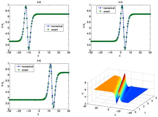
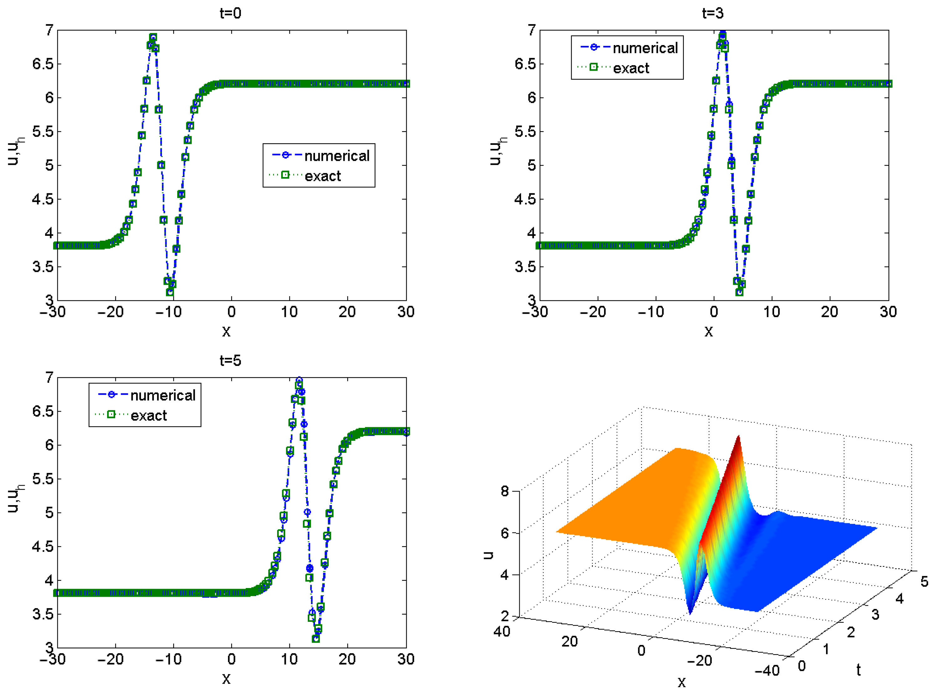
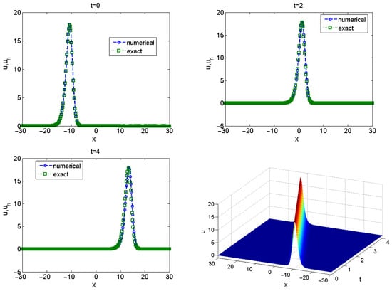
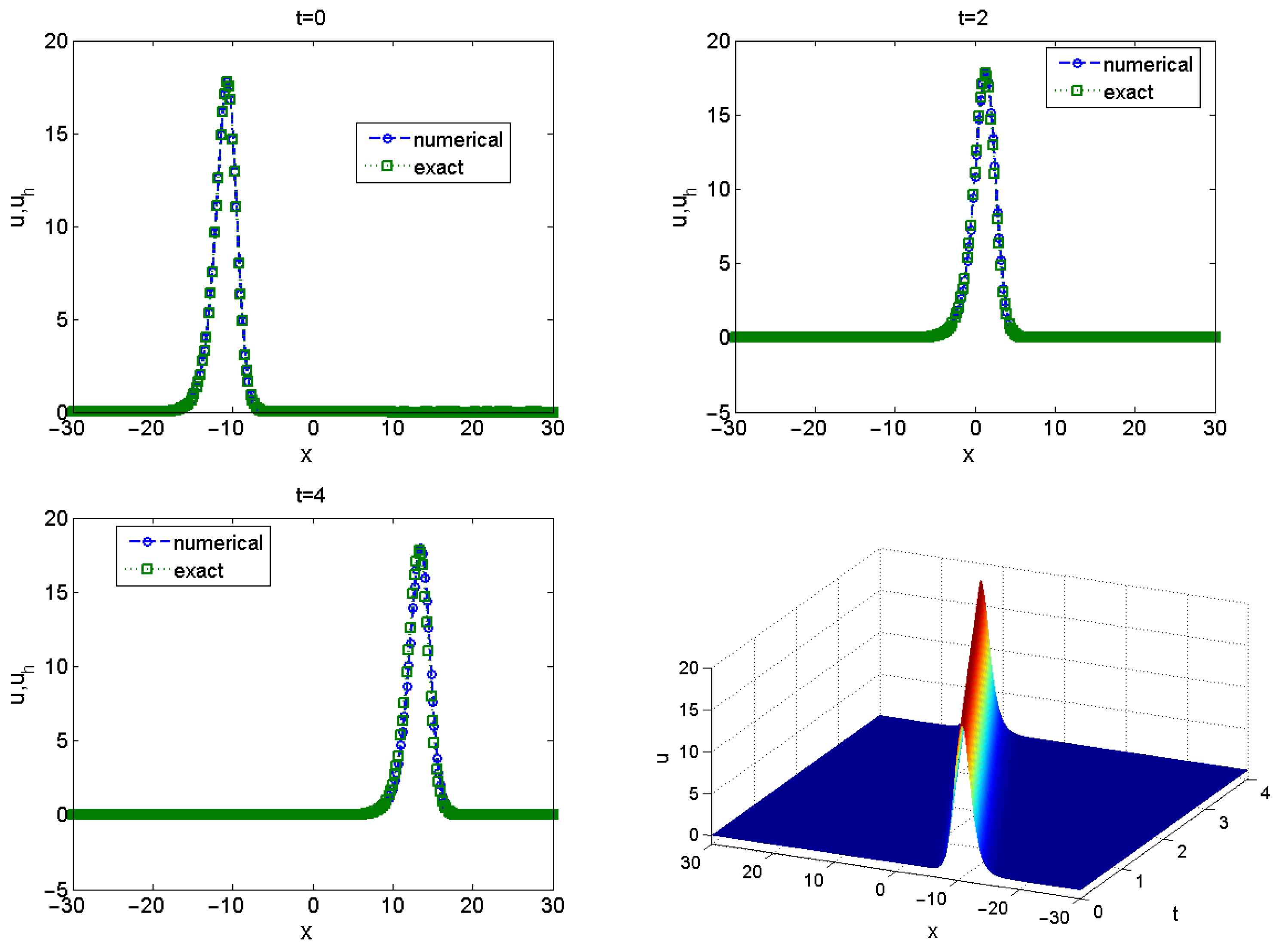
where $G_1$ and $G_2$ are obtained by (66) at $x=\pm 30$. We take the parameters $\theta =0.1$, $\lambda =\frac{1}{2}\sqrt{\frac{11}{19}}$, and $x_0=-10$ and the final time is $t=0.5$. Table 3, Table 4 and Table 5 report the $L^2$- and $L^{\infty }$-errors and the corresponding convergence orders for the multistep IMEX LDG schemes (25)–(27) on nonuniform meshes. In all tests, the time-step is chosen as $\tau =0.1\Delta x_{\min }$. Because the mesh and time-step are refined simultaneously, these tables report combined space–time convergence rather than a pure temporal-order test. The apparently third-order rate of the first-order formula for $N=2$ over the finest rows is a pre-asymptotic feature of this coupled space–time refinement and is not used to infer a temporal order. Over the reported meshes, the data indicate that the spatial contribution dominates the leading temporal contribution; the table itself cannot separate the two effects. Consistently, in Example 2 at $N=2$, $K=160$, the first-order and second-order $L^2$ errors begin to separate, taking the values $1.53\times {10}^{-7}$ and $8.33\times {10}^{-8}$, respectively. The independent periodic test in Section 5.1, rather than these coupled tables, is used to identify the temporal rates. We also present a simulation of the regular shock–profile wave propagation for the Kuramoto–Sivashinsky equation (65); see Figure 1. The initial condition is

$$u(x,0)=\theta +\frac{15}{19}\sqrt{\frac{11}{19}}\left[-9\tanh \left(\lambda (x-x_0)\right)+11{\tanh }^3\left(\lambda (x-x_0)\right)\right],$$

(68)

with parameters $\theta =5$, $\lambda =\frac{1}{2}\sqrt{11/19}$, and $x_0=-10$. The computed profiles remain sharp and propagate without visible spurious oscillations for the resolutions shown.

Table 3. $L^2$- and $L^{\infty }$-errors and observed combined space–time refinement orders for Example 1 with K elements and polynomial degree N. Computations use the first-order multistep IMEX–LDG scheme (Equation (25)) with parameters $\theta =0.1$, $\lambda =\frac{1}{2}\sqrt{11/19}$, and $x_0=-10$.

	K	${\mathbf{L}}^2$ Error	Order	${\mathbf{L}}^{\mathbf{\infty }}$ Error	Order
N = 1	20	$2.18\times {10}^{-2}$	–	$1.60\times {10}^{-2}$	–
	40	$8.68\times {10}^{-3}$	1.33	$4.46\times {10}^{-3}$	1.84
	80	$2.73\times {10}^{-3}$	1.67	$1.26\times {10}^{-3}$	1.82
	160	$9.70\times {10}^{-4}$	1.49	$2.91\times {10}^{-4}$	2.11
N = 2	20	$7.54\times {10}^{-3}$	–	$4.79\times {10}^{-3}$	–
	40	$1.38\times {10}^{-3}$	2.45	$7.23\times {10}^{-4}$	2.73
	80	$1.46\times {10}^{-4}$	3.24	$6.12\times {10}^{-5}$	3.56
	160	$1.93\times {10}^{-5}$	2.92	$4.83\times {10}^{-6}$	3.66

Table 4. $L^2$- and $L^{\infty }$-errors and observed combined space–time refinement orders for Example 1 with K elements and polynomial degree N. Computations use the second-order multistep IMEX–LDG scheme (Equation (26)) with parameters $\theta =0.1$, $\lambda =\frac{1}{2}\sqrt{11/19}$, and $x_0=-10$.

	K	${\mathbf{L}}^2$ Error	Order	${\mathbf{L}}^{\mathbf{\infty }}$ Error	Order
N = 1	20	$2.63\times {10}^{-2}$	–	$1.92\times {10}^{-2}$	–
	40	$9.40\times {10}^{-3}$	1.48	$5.02\times {10}^{-3}$	1.94
	80	$3.06\times {10}^{-3}$	1.62	$1.36\times {10}^{-3}$	1.89
	160	$1.04\times {10}^{-3}$	1.55	$3.09\times {10}^{-4}$	2.13
N = 2	20	$8.14\times {10}^{-3}$	–	$5.65\times {10}^{-3}$	–
	40	$1.41\times {10}^{-3}$	2.53	$7.01\times {10}^{-4}$	3.01
	80	$1.49\times {10}^{-4}$	3.24	$6.46\times {10}^{-5}$	3.44
	160	$1.94\times {10}^{-5}$	2.94	$5.58\times {10}^{-6}$	3.53

Table 5. $L^2$- and $L^{\infty }$-errors and observed combined space–time refinement orders for Example 1 with K elements and polynomial degree N. Computations use the third-order multistep IMEX–LDG scheme (Equation (27)) parameters $\theta =0.1$, $\lambda =\frac{1}{2}\sqrt{11/19}$, and $x_0=-10$.

	K	${\mathbf{L}}^2$ Error	Order	${\mathbf{L}}^{\mathbf{\infty }}$ Error	Order
N = 1	20	$3.16\times {10}^{-2}$	–	$2.28\times {10}^{-2}$	–
	40	$8.21\times {10}^{-3}$	1.94	$4.64\times {10}^{-3}$	2.30
	80	$3.05\times {10}^{-3}$	1.43	$1.39\times {10}^{-3}$	1.73
	160	$1.03\times {10}^{-3}$	1.57	$3.10\times {10}^{-4}$	2.17
N = 2	20	$8.13\times {10}^{-3}$	–	$5.77\times {10}^{-3}$	–
	40	$1.43\times {10}^{-3}$	2.51	$7.26\times {10}^{-4}$	2.99
	80	$1.49\times {10}^{-4}$	3.26	$6.47\times {10}^{-5}$	3.49
	160	$1.93\times {10}^{-5}$	2.95	$5.56\times {10}^{-6}$	3.54

Figure 1. The shock profile wave propagation for Example 1. Computations use the third-order multistep IMEX–LDG scheme (Equation (27)) with $N=3$, $K=40$ and parameters $\theta =5$, $\lambda =\frac{1}{2}\sqrt{11/19}$, and $x_0=-10$.

Example 2. 

Consider the KS equation

$$u_t+u{u}_x-u_{xx}+u_{xxxx}=0,$$

(69)

with exact solution

$$u(x,t)=\theta +\frac{15}{19}\sqrt{1/19}\left[-3\tanh \left(\lambda (x-\theta t-x_0)\right)+{\tanh }^3\left(\lambda (x-\theta t-x_0)\right)\right].$$

(70)

Impose exact Dirichlet data

$$u(-50,t)=f_1\left(t\right),u(50,t)=f_2\left(t\right),$$

(71)

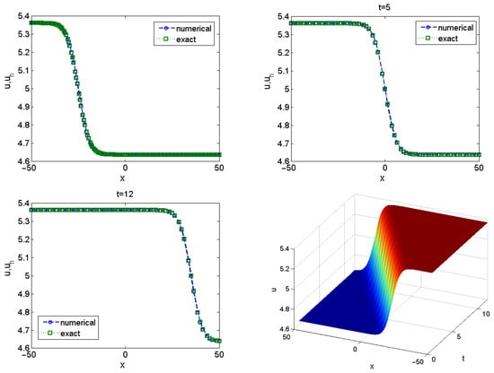
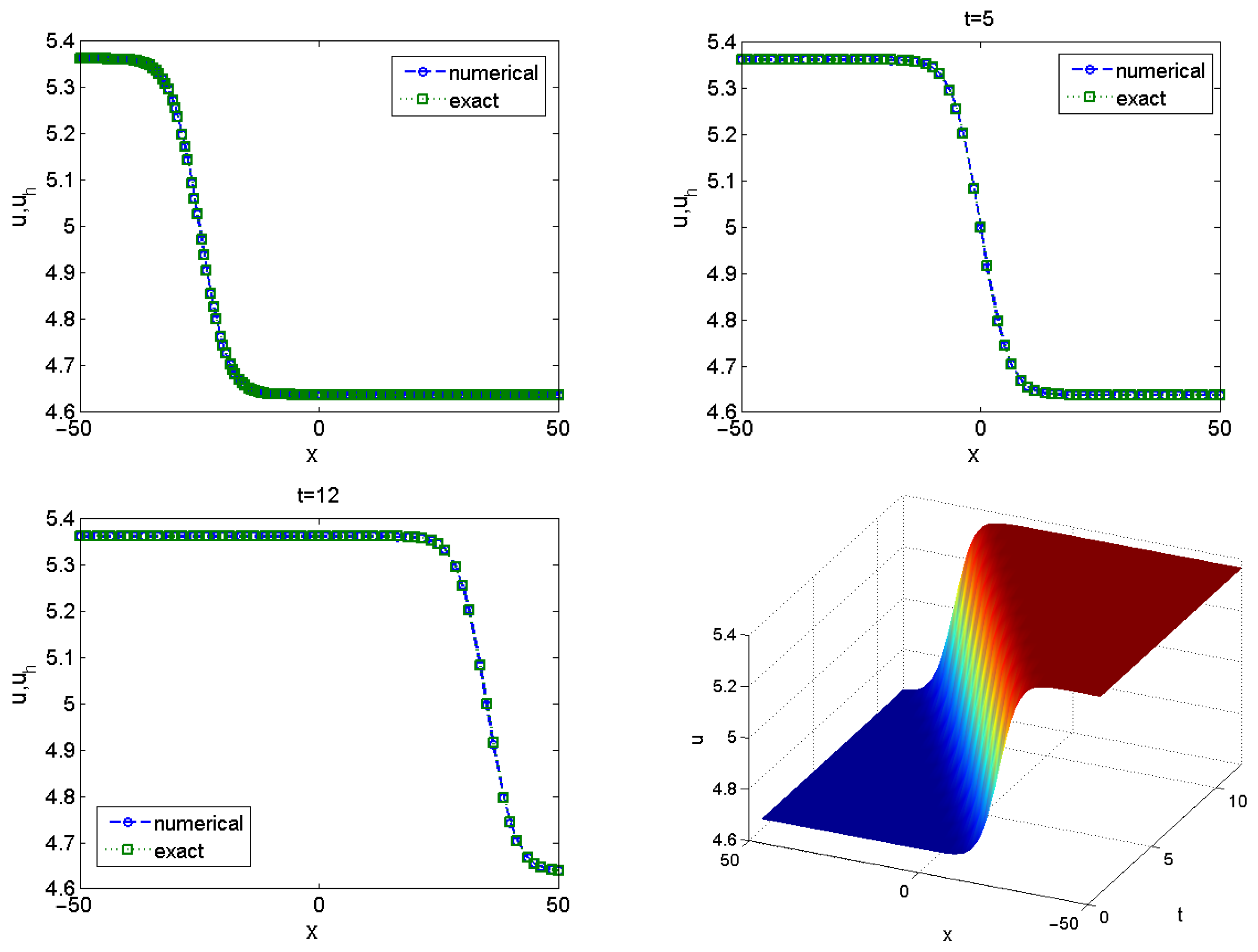
with $f_i\left(t\right)$ from (70). We take the parameters $\theta =0.2$, $\lambda =\frac{1}{2}\sqrt{\frac{1}{19}}$, and $x_0=-10$, and the final time is $t=1$. Table 6, Table 7 and Table 8 report the $L^2$- and $L^{\infty }$-errors and the corresponding convergence orders for the multistep IMEX LDG schemes (25)–(27) on nonuniform meshes. The tables show consistent decay of both error norms under refinement. Since space and time are refined together, the reported rates should be interpreted as combined space–time rates, with N denoting the polynomial degree of the DG space. The third-order entries in Table 8 are interpreted only as combined space–time refinement data. In particular, the $N=2$ entries are numerically almost identical to those of the second-order formula on the finest grids, so no temporal-order conclusion is drawn from this comparison. We also present a simulation of the regular shock-profile wave propagation for the Kuramoto–Sivashinsky equation (69); see Figure 2. The initial condition is

$$u(x,0)=\theta +\frac{15}{19}\sqrt{\frac{1}{19}}\left[-3\tanh \left(\lambda (x-x_0)\right)+{\tanh }^3\left(\lambda (x-x_0)\right)\right],$$

(72)

with parameters $\theta =5$, $\lambda =\frac{1}{2}\sqrt{1/19}$, and $x_0=-25$. The computed profiles remain sharp and propagate without visible spurious oscillations for the resolutions shown.

Table 6. $L^2$- and $L^{\infty }$-errors and observed combined space–time refinement orders for Example 2 with K elements and polynomial degree N. Computations use the first-order multistep IMEX–LDG scheme (Equation (25)) with parameters $\theta =0.2$, $\lambda =\frac{1}{2}\sqrt{1/19}$, and $x_0=-10$.

	K	${\mathbf{L}}^2$ Error	Order	${\mathbf{L}}^{\mathbf{\infty }}$ Error	Order
N = 1	20	$7.00\times {10}^{-4}$	–	$3.59\times {10}^{-4}$	–
	40	$1.53\times {10}^{-4}$	2.19	$6.27\times {10}^{-5}$	2.52
	80	$2.98\times {10}^{-5}$	2.36	$1.01\times {10}^{-5}$	2.63
	160	$6.58\times {10}^{-6}$	2.18	$1.83\times {10}^{-6}$	2.47
N = 2	20	$7.62\times {10}^{-5}$	–	$5.03\times {10}^{-5}$	–
	40	$9.38\times {10}^{-6}$	3.02	$5.48\times {10}^{-6}$	3.20
	80	$8.95\times {10}^{-7}$	3.39	$2.80\times {10}^{-7}$	4.29
	160	$1.53\times {10}^{-7}$	2.54	$3.78\times {10}^{-8}$	2.89

Table 7. $L^2$- and $L^{\infty }$-errors and observed combined space–time refinement orders for Example 2 with K elements and polynomial degree N. Computations use the second-order multistep IMEX–LDG scheme (26) with parameters $\theta =0.2$, $\lambda =\frac{1}{2}\sqrt{1/19}$, and $x_0=-10$.

	K	${\mathbf{L}}^2$ Error	Order	${\mathbf{L}}^{\mathbf{\infty }}$ Error	Order
N = 1	20	$7.36\times {10}^{-4}$	–	$4.07\times {10}^{-4}$	–
	40	$1.55\times {10}^{-4}$	2.25	$6.83\times {10}^{-5}$	2.57
	80	$3.07\times {10}^{-5}$	2.34	$1.09\times {10}^{-5}$	2.64
	160	$6.90\times {10}^{-6}$	2.15	$1.95\times {10}^{-6}$	2.49
N = 2	20	$7.75\times {10}^{-5}$	–	$5.19\times {10}^{-5}$	–
	40	$9.53\times {10}^{-6}$	3.02	$5.80\times {10}^{-6}$	3.16
	80	$8.73\times {10}^{-7}$	3.45	$3.67\times {10}^{-7}$	3.98
	160	$8.33\times {10}^{-8}$	3.39	$1.95\times {10}^{-8}$	4.24

Table 8. $L^2$- and $L^{\infty }$-errors and observed combined space–time refinement orders for Example 2 with K elements and polynomial degree N. Computations use the third-order multistep IMEX–LDG scheme (Equation (27)) with parameters $\theta =0.2$, $\lambda =\frac{1}{2}\sqrt{1/19}$, and $x_0=-10$.

	K	${\mathbf{L}}^2$ Error	Order	${\mathbf{L}}^{\mathbf{\infty }}$ Error	Order
N = 1	20	$7.79\times {10}^{-4}$	–	$4.65\times {10}^{-4}$	–
	40	$1.21\times {10}^{-4}$	2.69	$5.46\times {10}^{-5}$	3.09
	80	$2.60\times {10}^{-5}$	2.21	$9.52\times {10}^{-6}$	2.52
	160	$6.54\times {10}^{-6}$	1.99	$1.85\times {10}^{-6}$	2.36
N = 2	20	$7.63\times {10}^{-5}$	–	$5.10\times {10}^{-5}$	–
	40	$9.46\times {10}^{-6}$	3.01	$5.75\times {10}^{-6}$	3.15
	80	$8.72\times {10}^{-7}$	3.44	$3.66\times {10}^{-7}$	3.97
	160	$8.34\times {10}^{-8}$	3.38	$1.92\times {10}^{-8}$	4.25

Figure 2. The shock profile wave propagation for Example 2. Computations use the third-order multistep IMEX–LDG scheme (27) with $N=3$, $K=40$ and parameters $\theta =5$, $\lambda =\frac{1}{2}\sqrt{1/19}$, and $x_0=-25$.

Example 3. 

Consider the KS equation with third-derivative term

$$u_t+u{u}_x+u_{xx}+\beta u_{xxx}+u_{xxxx}=0,$$

(73)

with exact traveling-wave solution

$$u(x,t)=\theta +9-15\left(\tanh \left(\lambda (x-\theta t-x_0)\right)+{\tanh }^2\left(\lambda (x-\theta t-x_0)\right)-{\tanh }^3\left(\lambda (x-\theta t-x_0)\right)\right).$$

(74)

We take the parameters $\theta =0.2$, $\beta =4$, $\lambda =0.5$, $x_0=-10$ and the final time is $t=0.5$. Table 9 reports the $L^2$- and $L^{\infty }$-errors and the corresponding convergence orders for the multistep IMEX LDG schemes (26) and (27) on nonuniform meshes. The tables show consistent decay of both error norms under refinement. Since space and time are refined together, the reported rates should be interpreted as combined space–time rates, with N denoting the polynomial degree of the DG space. The third-order column is retained as combined space–time refinement data only and is not used to assess the pure temporal rate or Theorem 6. We also present a simulation of the regular shock-profile wave propagation for the Kuramoto–Sivashinsky equation with third-derivative term (73); see Figure 3. The initial condition is

$$u(x,0)=\theta +9-15\left[\tanh \left(\lambda (x-x_0)\right)+{\tanh }^2\left(\lambda (x-x_0)\right)-{\tanh }^3\left(\lambda (x-x_0)\right)\right].$$

(75)

with parameters $\theta =6$, $\beta =4$, $\lambda =0.5$, $x_0=-10$. The computed profiles remain sharp and propagate without visible spurious oscillations for the resolutions shown.

Table 9. $L^2$- and $L^{\infty }$-errors and observed combined space–time refinement orders for Example 3 with K elements and polynomial degree $N=2$. Computations use the second- and third-order multistep IMEX–LDG schemes, (26) and (27), with $\theta =0.2$, $\beta =4$, $\lambda =\frac{1}{2}$, and $x_0=-10$.

	K	${\mathbf{L}}^2$ Error	Order	${\mathbf{L}}^{\mathbf{\infty }}$ Error	Order
Second-order IMEX–LDG	40	$2.41\times {10}^{-2}$	–	$1.24\times {10}^{-2}$	–
scheme (26)	80	$3.14\times {10}^{-3}$	2.94	$1.15\times {10}^{-2}$	3.43
	160	$3.96\times {10}^{-4}$	2.98	$9.94\times {10}^{-5}$	3.54
Third-order IMEX–LDG	40	$3.00\times {10}^{-2}$	–	$1.52\times {10}^{-2}$	–
scheme (27)	80	$5.80\times {10}^{-3}$	2.37	$1.77\times {10}^{-3}$	3.10
	160	$9.33\times {10}^{-4}$	2.64	$1.97\times {10}^{-4}$	3.17

Figure 3. The shock profile wave propagation for Example 3. Computations use the third-order multistep IMEX–LDG scheme (27) with $N=3$, $K=40$ and parameters $\theta =6$, $\beta =4$, $\lambda =\frac{1}{2}$, and $x_0=-10$.

Example 4. 

We consider the classical Kuramoto–Sivashinsky equation

$$u_t+u{u}_x+u_{xx}+u_{xxxx}=0,$$

(76)

subject to periodic boundary conditions on a finite interval, a setting that produces spatio-temporal chaos. We test two standard initial conditions:

$$\begin{array}{cccc}\hfill u(x,0)& =\cos (x/16)(1+\sin (x/16\left)\right),\hfill & \hfill & x\in [0,32\pi ],\mathit{periodic},\hfill \end{array}$$

(77)

$$\begin{array}{cccc}\hfill u(x,0)& ={\mathrm{e}}^{-x^2},\hfill & \hfill & x\in [-30,30],\mathit{periodic}.\hfill \end{array}$$

(78)

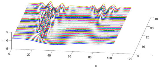
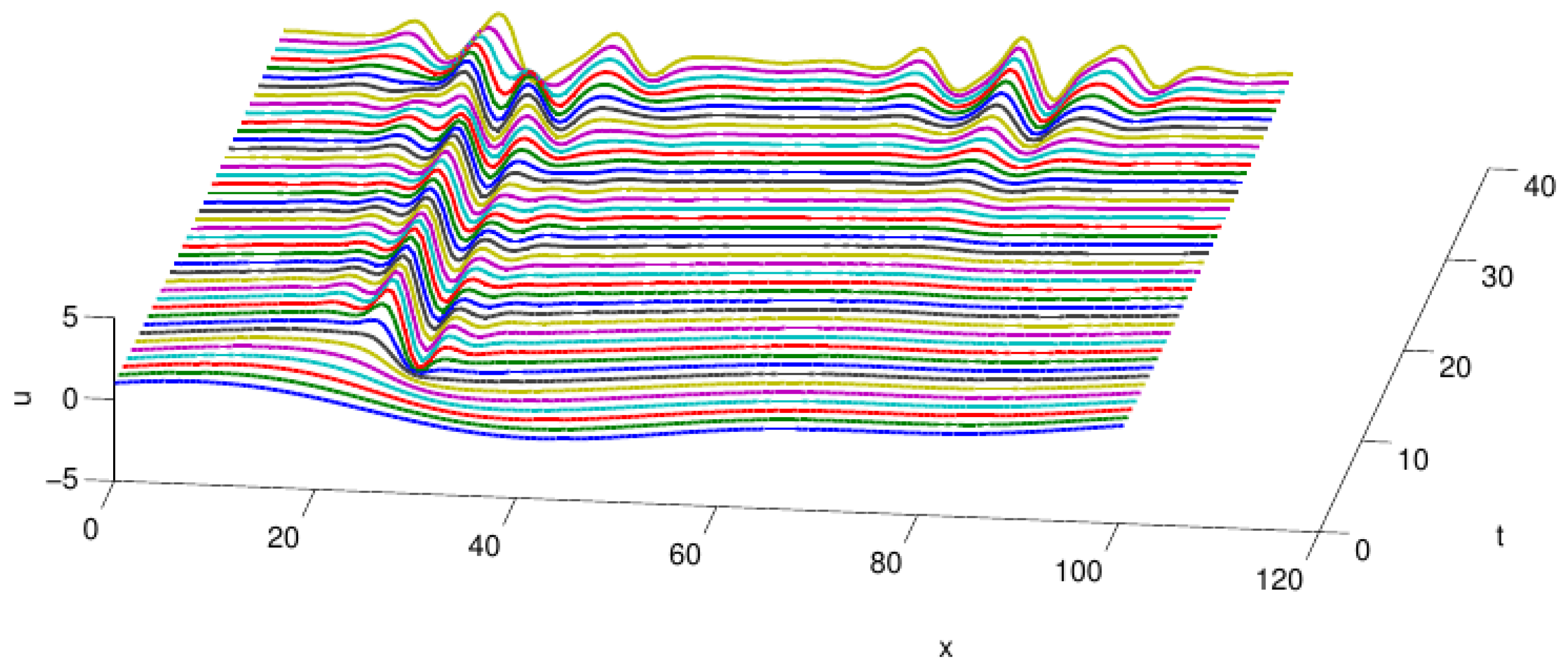
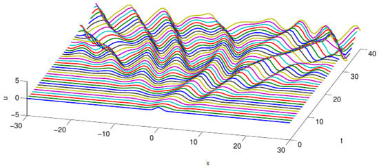
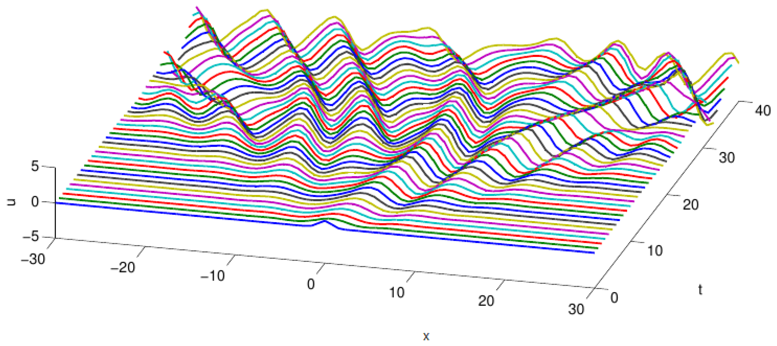
Figure 4 and Figure 5 display the numerical solutions and their space–time evolutions over the time interval $t\in [0,40]$. Figure 4 and Figure 5 show similar qualitative long-time space–time-structures. Because trajectories in a chaotic regime separate rapidly, these plots are not used as evidence of pointwise long-time convergence. Both figures use the coarser grid $K=80$ and are retained only as qualitative illustrations; no claim of high-wavenumber resolution is based on them. The quantitative diagnostics below assess time-step and spatial refinement using the numerical setup described above.

Figure 4. The chaotic solution of the KS equation for Example 4 with initial condition (77). Computations use the third-order multistep IMEX–LDG scheme (27) with $N=2$, $K=80$. The colored curves represent spatial solution profiles at successive time instants; the colors are used solely for visual distinction and have no additional quantitative meaning.

Figure 5. The chaotic solution of the KS equation for Example 4 with initial condition (78). Computations use the third-order multistep IMEX–LDG scheme (27) with $N=2$, $K=80$. The colored curves represent spatial solution profiles at successive time instants; the colors are used solely for visual distinction and have no additional quantitative meaning.

To supplement the qualitative space–time plots, we monitor the discrete energy

$$E_h\left(t\right)=\frac{1}{2}{\parallel u_h(·,t)\parallel }_{L^2\left(I\right)}^2.$$

(79)

The quantitative diagnostics use polynomial degree $N=2$ and the local Lax–Friedrichs numerical flux for the Burgers term. The starting states $u^1,u^2,u^3$ were generated by the high-accuracy stiff BDF initialization described at the beginning of this section, so the comparisons below are not affected by startup error.

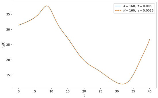
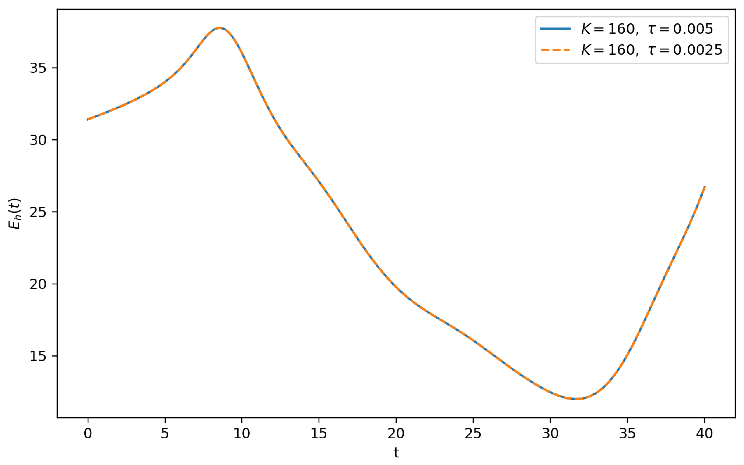
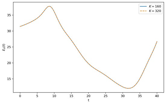
For time-step refinement we take $K=160$ and compare $\tau =0.005$ with $\tau =0.0025$. Over the finite observation window $20\le t\le 40$, the mean energies are $16.34649034$ and $16.34562849$, respectively, and the maximum difference between the energy histories sampled at the coarser time levels is $1.70\times {10}^{-6}$. The curves are therefore indistinguishable at the scale of Figure 6. The window average is used only as a finite-time diagnostic and is not interpreted as a stationary statistical mean.

Figure 6. Discrete energy history for Example 4 at $N=2$, $K=160$, comparing $\tau =0.005$ and $\tau =0.0025$.

For the spatial spectrum we evaluate each Fourier coefficient directly from the DG polynomial by elementwise Gaussian quadrature,

$$\widehat{u}(k_m,t_j)=\frac{1}{\left|I\right|}\sum _{K_e}{\int }_{K_e}{u}_h(x,t_j)e^{-i{k}_{m}x}dx,\overline{P}\left(k_m\right)=\frac{1}{N_s}{\displaystyle \sum _{j=1}^{N_s}}{\left|\widehat{u}(k_m,t_j)\right|}^2,$$

(80)

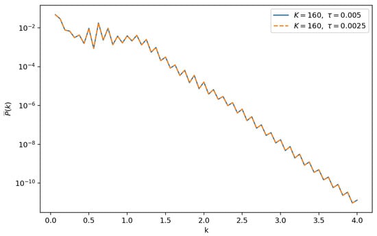
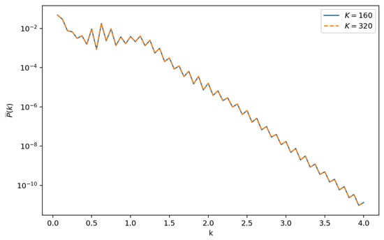
with $N_s=101$ snapshots over $20\le t\le 40$. This direct integration avoids additional point-sampling or reconstruction artifacts at element interfaces. Figure 7 compares the two time-steps at $K=160$. The relative ${\ell }^2$ difference over $0<k\le 4$ is $4.78\times {10}^{-8}$.

Figure 7. Time-averaged direct-DG spectrum for Example 4, comparing $\tau =0.005$ and $0.0025$ at $N=2$, $K=160$, averaged over $20\le t\le 40$.

The largest coefficient occurs at $k=0.0625=2\pi /L$, the fundamental box mode for $L=32\pi$. This does not mean that the linearly most unstable KS mode has shifted to the box scale: linearization about zero gives the growth rate $k^2-k^4$, whose maximum is at $k=1/\sqrt{2}\approx 0.707$. Rather, the reported spectrum is a finite-window spectrum of a nonlinear solution initialized with strong long-wave content; appreciable power is also visible in the band around the linearly active wavenumbers.

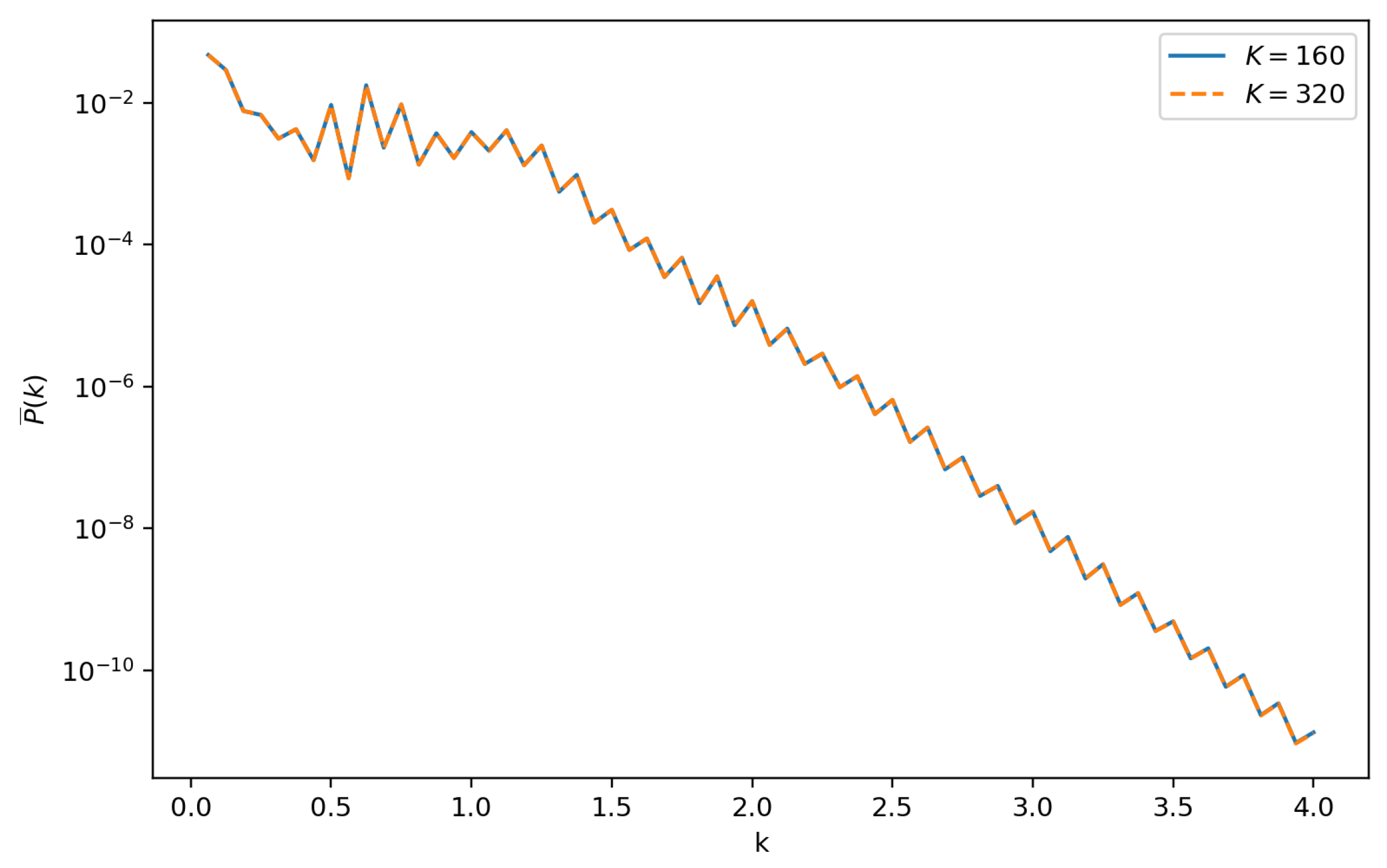
For spatial refinement we fix $\tau =0.0025$ and compare $K=160$ with $K=320$. The window-averaged energies are $16.34562849$ and $16.34553408$, and the maximum sampled energy difference over $20\le t\le 40$ is $7.43\times {10}^{-4}$. The direct-DG spectra have a relative ${\ell }^2$ difference of $1.82\times {10}^{-5}$ over $0<k\le 4$, while at $k=4$ the spectral powers are $1.33\times {10}^{-11}$ and $1.30\times {10}^{-11}$ for $K=160$ and $K=320$, respectively. Both spectra exhibit the expected strong decay of the dissipative tail, and their close agreement up to $k=4$ indicates that $K=160$ resolves the reported wavenumber band. The corresponding energy histories under spatial refinement are shown in Figure 8.

Figure 8. Energy histories under spatial refinement for Example 4: $K=160$ and $K=320$ with $N=2$ and $\tau =0.0025$.

The corresponding time-averaged direct-DG spectra under spatial refinement are presented in Figure 9.

Figure 9. Time-averaged direct-DG spectra under spatial refinement for Example 4: $K=160$ and $K=320$, $N=2$, $\tau =0.0025$, averaged over $20\le t\le 40$.

Example 5. 

Consider the KS equation

$$u_t+u{u}_x+u_{xx}+u_{xxxx}=0,$$

(81)

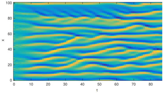
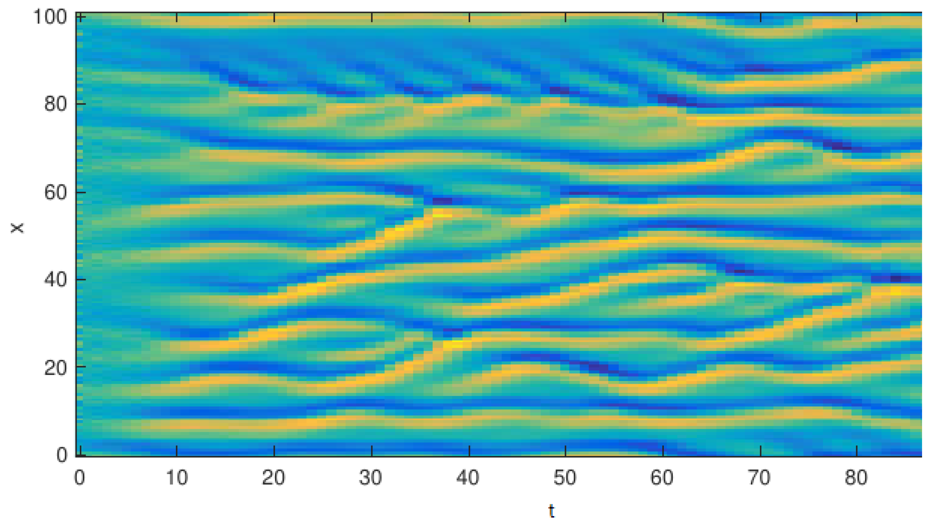
posed with periodic boundary conditions on $x\in [0,32\pi ]$. The displayed computation starts from values drawn uniformly from $[-1,1]$ at the discrete initialization points.

Figure 10 displays one numerical realization and its space–time evolution over $t\in [0,100]$. This displayed realization is used only as a qualitative long-time illustration; it is not used to verify Theorem 6 or an isolated third-order temporal rate. This experiment is used as a qualitative long-time robustness illustration of the third-order IMEX–LDG discretization in a chaotic regime; because of sensitivity to perturbations, no pointwise long-time convergence claim is inferred from this realization. Starting from random initial data, distinctly time-asymmetric patterns emerge: as time advances, slanted wave packets (“stripes”) repeatedly appear and merge, but do not split. In the visualization, color (or height) encodes the solution amplitude. Small random perturbations rapidly amplify and organize into traveling packets that continually form, interact, and coalesce. This birth–merger process is a hallmark of KS dynamics and signals the transition from transient pattern formation to sustained spatio-temporal chaos on long domains.

Figure 10. Chaotic solution of the Kuramoto–Sivashinsky equation for Example 5 with initial data given by independent and identically distributed random values at each grid point, uniformly distributed on $[-1,1]$, on the periodic domain $x\in [0,32\pi ]$ over $t\in [0,100]$. Computations use the third-order multistep IMEX–LDG scheme (27) with polynomial degree $N=3$ and $K=40$ elements. The colors represent the amplitude of the numerical solution $u(x,t)$ across the spatial and temporal domains.

6. Conclusions

We studied three multistep IMEX–LDG discretizations for nonlinear fourth-order time-dependent problems, using the Kuramoto–Sivashinsky equation as the principal model. Nonlinear convection is treated explicitly, whereas the linear second-, third-, and fourth-derivative terms are treated implicitly. Under the quasi-uniform mesh assumption and the uniform bounded-range hypothesis (19), the stability analysis gives $L^2$ bounds under a time-step condition $\tau \le {\tau }_0$ whose upper bound is independent of the mesh size, so no mesh-dependent CFL restriction is required by the estimates. Using a coupled LDG elliptic projection, we obtain the error bounds $O(h^{N+1}+\tau )$, $O(h^{N+1}+{\tau }^2)$, and $O(h^{N+1}+{\tau }^3)$ for the first-, second-, and third-order formulas, respectively, with the multistep results conditional on starting values of the corresponding accuracy.

The numerical experiments now separate temporal and spatial verification. The periodic manufactured temporal test recovers finest-refinement rates of approximately $1.00$, $2.01$, and $3.00$, while the $T=0.5$ spatial test of the third-order formula at $N=2$ gives an observed rate essentially equal to three. The traveling-wave tables remain useful combined space–time data, but their third-order columns are not used to verify Theorem 6. For the periodic KS diagnostics, $K=160$ is used as the baseline. Halving the time-step from $0.005$ to $0.0025$ changes the time-averaged direct-DG spectrum over $0<k\le 4$ by only $4.78\times {10}^{-8}$ in relative ${\ell }^2$ norm. At $\tau =0.0025$, refinement from $K=160$ to $K=320$ gives a relative spectral difference $1.82\times {10}^{-5}$ over the same band, and both spectra decay to approximately ${10}^{-11}$ at $k=4$. These results are interpreted as finite-window temporal and spatial resolution checks, not as evidence of pointwise long-time convergence or statistically stationary invariant measures.

The present analysis is deliberately one-dimensional. On tensor-product meshes in two dimensions, the LDG derivative chain and alternating traces can in principle be constructed direction by direction, and tensor-product analogues of one-dimensional projection estimates are available. The main additional difficulty is the simultaneous control of directional interface terms and nonlinear perturbations in a multidimensional discrete energy. On unstructured triangular meshes the extension is more substantial: one loses the simple one-dimensional coupled elliptic-projection/alternating-trace structure, face orientations must be incorporated consistently into alternating traces, and projection/error estimates must be rebuilt on element faces. For models such as the two-dimensional KS or Cahn–Hilliard equations, these issues are compounded by the multidimensional nonlinear operator and, in the latter case, the chemical-potential formulation. A rigorous two-dimensional extension is therefore left for future work rather than being inferred from the present one-dimensional theory.

References

- Hooper, A.P.; Grimshaw, R. Nonlinear instability at the interface between two viscous fluids. Phys. Fluids 1985, 28, 37–45. [Google Scholar] [CrossRef] [Scilit]
- Kuramoto, Y.; Tsuzuki, T. Persistent propagation of concentration waves in dissipative media far from thermal equilibrium. Prog. Theor. Phys. 1976, 55, 356–369. [Google Scholar] [CrossRef] [Scilit]
- Sivashinsky, G.I. Instabilities, pattern formation, and turbulence in flames. Annu. Rev. Fluid Mech. 1983, 15, 179–199. [Google Scholar] [CrossRef] [Scilit]
- Liu, X. Gevrey class regularity and approximate inertial manifolds for the Kuramoto–Sivashinsky equation. Phys. D Nonlinear Phenom. 1991, 50, 135–151. [Google Scholar] [CrossRef] [Scilit]
- Hyman, J.M.; Nicolaenko, B. The Kuramoto–Sivashinsky equation: A bridge between PDEs and dynamical systems. Phys. D Nonlinear Phenom. 1986, 18, 113–126. [Google Scholar] [CrossRef] [Scilit]
- Michelson, D. Steady solutions of the Kuramoto–Sivashinsky equation. Phys. D Nonlinear Phenom. 1986, 19, 89–111. [Google Scholar] [CrossRef] [Scilit]
- Gottlieb, S.; Ketcheson, D.I.; Shu, C.-W. Strong Stability Preserving Runge–Kutta and Multistep Time Discretizations; World Scientific: Singapore, 2011. [Google Scholar] [CrossRef] [Scilit]
- Cockburn, B.; Shu, C.-W. Runge–Kutta discontinuous Galerkin methods for convection-dominated problems. J. Sci. Comput. 2001, 16, 173–261. [Google Scholar] [CrossRef] [Scilit]
- Cockburn, B.; Shu, C.-W. The local discontinuous Galerkin method for time-dependent convection-diffusion systems. SIAM J. Numer. Anal. 1998, 35, 2440–2463. [Google Scholar] [CrossRef] [Scilit]
- Bassi, F.; Rebay, S. A high-order accurate discontinuous finite element method for the numerical solution of the compressible Navier–Stokes equations. J. Comput. Phys. 1997, 131, 267–279. [Google Scholar] [CrossRef] [Scilit]
- Arnold, D.N.; Brezzi, F.; Cockburn, B.; Marini, L.D. Unified analysis of discontinuous Galerkin methods for elliptic problems. SIAM J. Numer. Anal. 2002, 39, 1749–1779. [Google Scholar] [CrossRef] [Scilit]
- Yan, J.; Shu, C.-W. A local discontinuous Galerkin method for KdV type equations. SIAM J. Numer. Anal. 2002, 40, 769–791. [Google Scholar] [CrossRef] [Scilit]
- Cockburn, B.; Kanschat, G.; Schötzau, D.; Schwab, C. Local discontinuous Galerkin methods for the Stokes system. SIAM J. Numer. Anal. 2002, 40, 319–343. [Google Scholar] [CrossRef] [Scilit]
- Dong, B.; Shu, C.-W. Analysis of a local discontinuous Galerkin method for linear time-dependent fourth-order problems. SIAM J. Numer. Anal. 2009, 47, 3240–3268. [Google Scholar] [CrossRef] [Scilit]
- Yan, J.; Osher, S. A local discontinuous Galerkin method for directly solving Hamilton–Jacobi equations. J. Comput. Phys. 2011, 230, 232–244. [Google Scholar] [CrossRef] [Scilit]
- Xu, Y.; Shu, C.-W. Local discontinuous Galerkin methods for the Kuramoto–Sivashinsky equations and the Ito-type coupled KdV equations. Comput. Methods Appl. Mech. Eng. 2006, 195, 3430–3447. [Google Scholar] [CrossRef] [Scilit]
- Akrivis, G.; Smyrlis, Y.S. Implicit–explicit BDF methods for the Kuramoto–Sivashinsky equation. Appl. Numer. Math. 2004, 51, 151–169. [Google Scholar] [CrossRef] [Scilit]
- Kassam, A.-K.; Trefethen, L.N. Fourth-order time-stepping for stiff PDEs. SIAM J. Sci. Comput. 2005, 26, 1214–1233. [Google Scholar] [CrossRef] [Scilit]
- Hundsdorfer, W.; Verwer, J.G. Numerical Solution of Time-Dependent Advection-Diffusion-Reaction Equations; Volume 33 of Springer Series in Computational Mathematics; Springer: Berlin/Heidelberg, Germay, 2003. [Google Scholar] [CrossRef] [Scilit]
- Ascher, U.M.; Ruuth, S.J.; Spiteri, R.J. Implicit-explicit Runge–Kutta methods for time-dependent partial differential equations. Appl. Numer. Math. 1997, 25, 151–167. [Google Scholar] [CrossRef] [Scilit]
- Wang, H.; Shu, C.-W.; Zhang, Q. Stability and error estimates of local discontinuous Galerkin methods with implicit-explicit time-marching for advection-diffusion problems. SIAM J. Numer. Anal. 2015, 53, 206–227. [Google Scholar] [CrossRef] [Scilit]
- Wang, H.; Shu, C.-W.; Zhang, Q. Stability analysis and error estimates of local discontinuous Galerkin methods with implicit–explicit time-marching for nonlinear convection–diffusion problems. Appl. Math. Comput. 2016, 272, 237–258. [Google Scholar] [CrossRef] [Scilit]
- Wang, H.; Zhang, Q.; Shu, C.-W. Stability analysis and error estimates of local discontinuous Galerkin methods with implicit-explicit time-marching for the time-dependent fourth order PDEs. ESAIM Math. Model. Numer. Anal. 2017, 51, 1931–1955. [Google Scholar] [CrossRef] [Scilit]
- Zhang, L. A local energy-based discontinuous Galerkin method for fourth-order semilinear wave equations. IMA J. Numer. Anal. 2024, 44, 2793–2820. [Google Scholar] [CrossRef] [Scilit]
- Lin, G.; Zhang, D.; Li, J.; Wu, B. An ultra-weak local discontinuous Galerkin method with generalized numerical fluxes for the KdV–Burgers–Kuramoto equation. J. Sci. Comput. 2024, 99, 65. [Google Scholar] [CrossRef] [Scilit]
- Li, L.; Meng, X.; Li, J. Analysis of the local discontinuous Galerkin method with generalized numerical fluxes for one-dimensional nonlinear fourth-order time-dependent problems. J. Sci. Comput. 2025, 102, 72. [Google Scholar] [CrossRef] [Scilit]
- Li, L.; Meng, X.; Wu, B. Superconvergence of the local discontinuous Galerkin method with generalized numerical fluxes for one-dimensional nonlinear time-dependent fourth-order equations. Commun. Comput. Phys. 2026, 40, 1053–1103. [Google Scholar] [CrossRef] [Scilit]
- Zhou, L.; Chen, W.; Guo, R. Stability and error estimates of ultra-weak local discontinuous Galerkin method with spectral deferred correction time-marching for PDEs with high order spatial derivatives. J. Comput. Math. 2026, 44, 286–306. [Google Scholar] [CrossRef] [Scilit]
- Fu, F.; Shu, C.-W.; Tao, Q.; Wu, B. Analysis of the boundary conditions for the ultraweak-local discontinuous Galerkin method of time-dependent linear fourth-order problems. Math. Comput. 2025, 94, 123–158. [Google Scholar] [CrossRef] [Scilit]
- Fu, F.; Shu, C.-W.; Tao, Q. The ultraweak-local discontinuous Galerkin method for extended Fisher–Kolmogorov equations. J. Comput. Appl. Math. 2026, 475, 117023. [Google Scholar] [CrossRef] [Scilit]
- Liu, Y.; Cheng, Y. Local discontinuous Galerkin method for a singularly perturbed fourth-order problem of reaction–diffusion type. J. Comput. Appl. Math. 2024, 440, 115641. [Google Scholar] [CrossRef] [Scilit]
- Liu, Y.; Wang, X.; Cheng, Y. Local discontinuous Galerkin method for a singularly perturbed fourth-order problem of convection–diffusion type. Appl. Numer. Math. 2024, 205, 16–37. [Google Scholar] [CrossRef] [Scilit]
- Doss, L.J.T.; Kousalya, N. A finite pointset method for Kuramoto–Sivashinsky equation based on mixed formulation. Math. Methods Appl. Sci. 2025, 48, 765–778. [Google Scholar] [CrossRef] [Scilit]
- Doss, L.J.T.; Sindhujarani, V. H1-Galerkin mixed finite element method using tensor product of cubic B-splines for two-dimensional Kuramoto–Sivashinsky equation. Comput. Math. Appl. 2025, 188, 19–39. [Google Scholar] [CrossRef] [Scilit]
- Choudhary, R.; Singh, S.; Das, P.; Kumar, D. A higher order stable numerical approximation for time-fractional non-linear Kuramoto–Sivashinsky equation based on quintic B-spline. Math. Methods Appl. Sci. 2024, 47, 11953–11975. [Google Scholar] [CrossRef] [Scilit]
- Jiang, H.; Xu, D. A fast high-order compact difference scheme for time-fractional KS equation with the generalized Burgers’ type nonlinearity. Fractal Fract. 2025, 9, 218. [Google Scholar] [CrossRef] [Scilit]
- Aboelenen, T.; Zaky, M.A.; Aljurbua, S.F. An arbitrary Lagrangian–Eulerian local discontinuous Galerkin method with implicit–explicit time discretization for nonlinear fourth-order problems on moving meshes. Appl. Numer. Math. 2027, 231, 155–183. [Google Scholar] [CrossRef] [Scilit]
- Kanevsky, A.; Carpenter, M.H.; Gottlieb, D.; Hesthaven, J.S. Application of implicit–explicit high order Runge–Kutta methods to discontinuous-Galerkin schemes. J. Comput. Phys. 2007, 225, 1753–1781. [Google Scholar] [CrossRef] [Scilit]
- Gu, X.-M.; Quan, C.; Xin, Q. Stability and convergence of implicit-explicit Runge–Kutta methods for the reaction-diffusion equation with random diffusion coefficient. Commun. Nonlinear Sci. Numer. Simul. 2026, 155, 109602. [Google Scholar] [CrossRef] [Scilit]
- Li, X.; Qiao, Z.; Zheng, N. Linear and decoupled IMEX schemes for the Ericksen–Leslie model: Unconditional stability, length-preserving and rigorous error analysis. Commun. Comput. Phys. 2026, 40, 1317–1346. [Google Scholar] [CrossRef] [Scilit]
- Zhan, H.; Wang, T.; Hu, G. An unconditionally energy-stable and orthonormality-preserving scheme for the Kohn–Sham gradient flow based model based on a tetrahedral spectral element method. Commun. Comput. Phys. 2025, 37, 921–941. [Google Scholar] [CrossRef] [Scilit]
- Zhu, H.; Yang, L.; Zhang, R.; Jia, Y. A coupled numerical method for time-fractional convection-diffusion equations based on compressed Legendre polynomials. AIMS Math. 2026, 11, 19488–19515. [Google Scholar] [CrossRef] [Scilit]
- Kant, K.; Das, P.; Nelakanti, G.; Kumar, R. Modified Galerkin method for derivative dependent Fredholm–Hammerstein integral equations of second kind. Adv. Appl. Math. Mech. 2024, 16, 905–926. [Google Scholar] [CrossRef] [Scilit]
- Jiang, G.-S.; Shu, C.-W. On a cell entropy inequality for discontinuous Galerkin methods. Math. Comput. 1994, 62, 531–538. [Google Scholar] [CrossRef]
Disclaimer/Publisher’s Note: The statements, opinions and data contained in all publications are solely those of the individual author(s) and contributor(s) and not of MDPI and/or the editor(s). MDPI and/or the editor(s) disclaim responsibility for any injury to people or property resulting from any ideas, methods, instructions or products referred to in the content. |
© 2026 by the authors. Licensee MDPI, Basel, Switzerland. This article is an open access article distributed under the terms and conditions of the Creative Commons Attribution (CC BY) license.