


Abstract
Multi-step water quality prediction comprises a set of related forecasting tasks whose information structure, uncertainty, and relative model competence vary with forecast horizon, monitoring context, and system state. Conventional model comparison commonly relies on performance averaged across lead times, which can obscure horizon-dependent error accumulation, model-ranking crossover, and regime-specific failure. This review examines adaptive horizon-aware model selection and routing from a mathematical and statistical perspective. Recursive, direct, multi-output, ensemble, mixture-of-experts, and adaptive routing strategies are compared according to their dependence structure, parameter sharing, loss coupling, and error-propagation mechanisms. Particular emphasis is placed on conditional risk as a unified representation of model competence across monitoring sections, temporal resolutions, target indicators, forecast horizons, and environmental states. Routing regret, competence margins, and selection uncertainty are further discussed to characterize the potential gain, stability, and reliability of conditional model allocation. The review also analyzes how hydrological memory, transport delay, cross-indicator dependence, external forcing, data scarcity, and concept drift reshape predictability across horizons. Statistical evaluation is considered through leakage-free temporal validation, rolling-origin assessment, dependence-aware model comparison, model-ranking uncertainty, probabilistic calibration, and selective prediction. This synthesis provides a mathematically structured basis for understanding when different forecasting mechanisms remain reliable and how horizon-dependent model competence can support more robust adaptive routing in multi-step water quality prediction.
Keywords:
multi-step water quality prediction; horizon-aware model selection; adaptive routing; conditional risk; routing regret; error propagation; model selection uncertainty; statistical inference MSC:
62M20
1. Introduction
Water quality forecasting supports pollution early warning, drinking-water protection, reservoir operation, watershed management, and treatment-process control [1,2]. With the increasing availability of continuous monitoring and multivariate environmental data, forecasting tasks have gradually expanded from single-step prediction toward multi-step and multi-horizon prediction [3,4,5,6]. The nature of these forecasting tasks varies across lead times. Hour-ahead, day-ahead, and longer-range forecasts differ in the persistence of historical information, the influence of external forcing, and the uncertainty associated with future states. Multi-step water quality forecasting should therefore be regarded as a set of related prediction tasks whose information structure and forecasting difficulty vary with horizon.
Forecast horizon changes the dependence between current observations and future water quality states. At short lead times, recent measurements often retain substantial predictive information through temporal persistence, transport continuity, and delayed system responses. As lead time increases, the influence of the initial state generally weakens, while rainfall, temperature, upstream conditions, seasonal variation, and hydrological regulation become more important [7]. This transition varies across indicators and monitoring systems. Process responses may also vary across chemical regimes such as water alkalinity [8]. Some variables preserve relatively stable temporal patterns, whereas others respond rapidly to runoff, pollutant inputs, or abrupt environmental disturbances [9]. Consequently, forecast horizon can affect predictor relevance, uncertainty growth, attainable accuracy, and the relative competence of competing models [10].
However, horizon-resolved evaluation remains comparatively limited in the current water-quality forecasting literature. Existing multi-step studies further show that relative model performance can change with lead time, as different forecasting strategies exhibit distinct degradation patterns across the forecast range [7,10,11]. Averaging performance across horizons can therefore mask error growth and model-ranking crossovers, while inappropriate temporal splitting, overlapping samples, full-series preprocessing, inconsistent horizon definitions, and weak baseline design can further distort apparent improvements [12].
The mathematical differences among multi-step forecasting strategies are closely related to output dependence, parameter sharing, and error transmission. Recursive forecasting repeatedly uses previous predictions to generate subsequent outputs and may therefore accumulate errors as the horizon increases. Direct forecasting avoids recursive feedback by estimating separate mappings for different future steps, while multi-output approaches jointly estimate several future states and preserve cross-horizon dependence [5]. Ensemble methods combine complementary predictive mechanisms, but their effectiveness depends on the stability and diversity of component models [7]. These structural differences indicate that no forecasting strategy should be assumed to remain optimal across all horizons.
Horizon-specific modelling, dynamic model selection, mixture-of-experts, and adaptive routing provide a more flexible alternative [11,13]. Rather than assigning one model to all forecasting conditions, model allocation can depend on forecast horizon, monitoring site, target indicator, recent water quality dynamics, hydrological state, data completeness, and external information. The central question therefore shifts from identifying the model with the lowest overall error to determining where and when different predictive mechanisms remain reliable. Conditional risk, model competence, routing regret, competence margin, and selection uncertainty provide a mathematical basis for describing these differences and evaluating whether adaptive allocation is justified.
Existing reviews of water-quality forecasting have primarily organized the literature around machine learning and deep learning architectures, prediction targets, and application settings [2], whereas the broader multi-step forecasting literature has focused on recursive, direct, multiple-output, and related forecasting strategies [14]. Dynamic model-selection and ensemble studies have further examined adaptive model allocation and combination largely outside water-quality applications [13,15]. These research streams have therefore remained only partially connected. The contribution of this review is not to propose new forecasting theories, but to integrate these established concepts into a unified horizon-aware framework for multi-step water-quality prediction. The conceptual structure of this framework is summarized in Figure 1. Specifically, the review links forecasting structure and error propagation with conditional model competence, adaptive routing, routing regret, selection stability, dependence-aware evaluation, and predictive uncertainty. This perspective shifts the central question from identifying a model with the best average performance to determining which forecasting mechanism remains reliable at a given horizon and context, and what evidence is required to support that allocation.
Figure 1.
Mathematical framework for adaptive horizon-aware model selection and trustworthy evaluation in multi-step water quality forecasting. (1) Forecasting tasks are defined by horizon, monitoring context, target variables, temporal resolution, and available information. (2) Horizon-dependent changes in information relevance and uncertainty lead to differences in the competence of candidate forecasting models. (3) Adaptive routing uses observable context to select the most appropriate model or model combination. (4) Horizon-resolved performance, routing regret, selection uncertainty, and statistically valid evaluation are used to determine whether the resulting allocation is reliable.
2. Review Methodology and Literature Selection
This review adopted a structured narrative approach to examine the mathematical and statistical foundations of multi-step water-quality forecasting and adaptive horizon-aware model selection. Relevant publications were searched in the Web of Science Core Collection and Scopus, with Google Scholar used as a supplementary source for recent and highly relevant studies. The final search was updated on 2 September 2026. Search terms combined water-quality descriptors, including “water quality”, “water quality index”, “dissolved oxygen”, “nutrient”, “turbidity”, and “chlorophyll”, with forecasting terms such as “forecasting”, “prediction”, “multi-step”, “multi-horizon”, “recursive”, “direct”, “MIMO”, “ensemble”, “dynamic model selection”, “adaptive model selection”, and “mixture of experts”. The main publication window covered 2015–2026, while earlier studies were retained when they provided foundational formulations or evaluation principles directly relevant to the review.
Studies were included when they either examined water-quality prediction across multiple future horizons or provided methodological foundations for multi-step forecasting, model selection, routing, uncertainty quantification, or forecast evaluation. Studies focusing solely on water-quality assessment, classification, spatial interpolation, or environmental-process analysis without a forecasting component were excluded. Records were screened according to their relevance to horizon-dependent forecasting and the mathematical framework developed in this review. The final synthesis incorporated 83 cited publications spanning empirical water-quality forecasting, general forecasting methodology, statistical evaluation, and related environmental applications. These 83 publications constitute the full evidence base of the integrative review, including both direct water-quality forecasting studies and methodological or adjacent-domain studies, and therefore were not treated as a denominator for estimating the prevalence of multi-horizon evaluation within water-quality forecasting studies.
To distinguish the strength and role of different evidence, the literature was classified into three evidence tiers. Tier 1 comprises 20 direct water-quality forecasting studies and provides the empirical basis for conclusions regarding forecasting performance and model comparison. The complete Tier 1 study set and its classification by forecasting horizon and model-allocation strategy are provided in Supplementary Table S1. Tier 2 includes general forecasting, statistical, and machine learning studies used to establish theoretical and methodological concepts. Tier 3 contains studies from adjacent environmental or engineering domains and is used only for methodological illustration or contextual interpretation when equivalent water-quality evidence is unavailable. Claims regarding the effectiveness of horizon-aware model selection or routing in water-quality forecasting are therefore based only on Tier 1 evidence, whereas Tier 2 and Tier 3 studies are used to support methodological formulation rather than empirical superiority.
3. Mathematical Structure of Multi-Step Water Quality Forecasting
3.1. Forecasting Task and Horizon Representation
Multi-step water quality forecasting can be formulated as a sequence prediction problem defined by a forecast origin, an available information set, a target variable, and a set of future lead times. The mathematical formulation should distinguish these elements from the forecasting model itself, because different model architectures may operate on the same forecasting task while imposing different dependence structures across future outputs. For a monitoring system containing q observed water quality variables, the state at time t is represented as
Here, Yt denotes the water quality state observed at time t, is the observation of the j-th water quality variable, j = 1,…, q, and q is the number of variables considered in the monitoring system. The formulation allows a forecasting task to involve either one target variable or several jointly predicted variables.
The information available when a forecast is issued can be written as
Ft = (Y1:t,X1:t),
In Equation (2), Ft denotes the information set available at forecast origin t, Y1:t contains historical water quality observations up to time t, and X1:t represents exogenous information available by that time, such as hydrological, meteorological, spatial, or operational variables. In engineered treatment systems, material configuration may also form part of the relevant process state when it directly affects the measured response [16]. If forecasts of future forcing variables are used, they should be regarded as part of Ft only when those forecasts would genuinely have been available at the corresponding forecast origin. For treatment-process applications, reagent and operating conditions can likewise constitute task-specific information when they govern multiple water-quality responses [17]. This definition prevents future observations from being implicitly included in the mathematical forecasting problem.
For a candidate model m, prediction at horizon h can then be represented by
Here, is the prediction generated by candidate model m for time t + h, fm denotes the corresponding forecasting mapping, and h is the forecast step measured from the forecast origin. Equation (3) makes horizon an explicit component of the forecasting problem rather than treating the complete output sequence as a single prediction. Multi-horizon architectures can still generate several future values simultaneously, but their performance remains resolvable at individual lead times [18].
The forecast step should also be distinguished from physical forecast lead time. For data sampled at a constant interval,
τh = hΔt.
In Equation (4), τh is the physical lead time associated with forecast step h, and Δt is the sampling interval. This distinction is necessary when comparing forecasting studies using different temporal resolutions. For example, the same numerical value of h represents different physical forecasting ranges in hourly and daily datasets. Consequently, both forecast step and sampling resolution should be reported when horizon-dependent performance is compared.
For multi-site and multi-indicator forecasting, the prediction problem can be further indexed by a task unit,
u = (s,δ,j,g),
Here, u denotes a forecasting task, s identifies the monitoring section or site, δ denotes temporal resolution, j identifies the target water quality indicator, and g denotes a forecast horizon or a predefined group of adjacent horizons. This representation does not assume that different tasks are independent. Historical information may be shared across indicators, sites, or temporal scales, and common representations may be learned from related tasks. Instead, Equation (5) defines the unit at which forecasting performance and model competence can be evaluated. This distinction becomes important when the same model is not expected to be equally suitable for every combination of site, indicator, temporal resolution, and forecast range.
3.2. Dependency Structure and Error Propagation
Multi-step forecasting strategies differ primarily in how future outputs depend on previous predictions, how parameters are shared across horizons, and how errors can propagate through the forecast sequence. Recursive, direct, and multiple-output strategies provide the main mathematical structures for this comparison [14,19]. These strategies have also been explicitly compared in multi-step water quality forecasting, where their relative performance changes with forecast construction and lead time [20,21].
Recursive forecasting repeatedly applies a common forecasting mechanism. A general representation is
In Equation (6), f denotes the recursively reused forecasting function, θ is its parameter set, H is the maximum forecast horizon, and denotes previously generated predictions that are available when the h-step forecast is produced. For h = 1, no previous predicted output is required. Recursive forecasting therefore achieves strong parameter sharing because the same transition mechanism is reused across the forecast sequence. Its defining limitation is that later predictions can depend on earlier model-generated values. The classical multi-step forecasting literature identifies this feedback mechanism as a major pathway for accumulated forecast error [14], and water quality comparisons of Recursive, Direct, DirREC, MIMO, and related strategies have reported different degradation patterns as the prediction range increases [20]. The general distinction among recursive, direct, and multiple-output strategies is well established in the multi-step forecasting literature.
Direct forecasting removes this recursive feedback by estimating a separate forecasting relationship for each horizon:
Here, fh denotes the forecasting function constructed specifically for horizon h, and θh is its horizon-specific parameter set. Because prediction at horizon h does not require predictions from earlier horizons as inputs, direct forecasting avoids recursive error transmission. The corresponding cost is that up to H separate forecasting relationships may need to be estimated. This increases parameter duplication and may weaken coherence among neighboring future predictions. Direct forecasting therefore exchanges strong parameter sharing for greater horizon specificity [14].
Multiple-output forecasting instead generates the future sequence through a joint mapping:
In Equation (8), ε denotes a joint multi-output forecasting mapping and θ contains the parameters shared by the joint model. Unlike recursive forecasting, previous predicted outputs do not have to be returned sequentially as inputs. Unlike direct forecasting, however, the future horizons are not estimated independently. Their dependence is represented through a common model and shared parameters. The MIMO strategy was developed specifically to preserve dependence among future predictions within a multiple-output formulation, and subsequent multi-horizon architectures have extended this principle using shared representations, attention mechanisms, and multiple output heads [22,23].
Joint prediction introduces cross-horizon interaction through the training objective. A general multi-horizon loss can be expressed as
Here, L is the aggregate training loss, ℓ(·,·) is the loss evaluated at an individual horizon, and ωh is the weight assigned to horizon h. The weights are written as non-negative values summing to one so that they can be interpreted as relative contributions of individual horizons to the overall objective. This normalization is convenient rather than mathematically necessary, because multiplying the complete objective by a positive constant does not change its minimizer.
Uniform weighting assigns the same nominal contribution to each horizon, but it does not guarantee equivalent learning difficulty or predictive performance. Horizons may differ in variance, noise, predictability, and effective sample information. A joint model can therefore achieve a favorable aggregate objective while retaining comparatively large errors at particular distant horizons. Horizon-dependent weighting, separate prediction heads, and multi-objective optimization represent alternative ways of controlling this coupling, but each introduces an explicit assumption about how errors at different lead times should be balanced.
Ensemble forecasting introduces a different form of dependence by combining predictions from several candidate models. A fixed horizon-specific ensemble can be written as
In Equation (10), M is the number of component models, wm,h is the weight assigned to model m at horizon h, and is the prediction produced by that model. The notation wm,h is deliberately distinguished from the horizon loss weight wh in Equation (9). The former determines how model predictions are combined, whereas the latter determines how prediction errors at different horizons contribute to model training.
The component models in Equation (10) may themselves use recursive, direct, or multiple-output structures. Consequently, an ensemble partly inherits the error properties of its constituent models. Horizon-specific weights allow the relative contribution of the models to change with lead time, but fixed weights remain unchanged across forecast origins within the same horizon. This is the principal structural distinction between fixed ensemble forecasting and the conditional allocation mechanisms considered in Section 3.
Recursive error transmission can be characterized more explicitly using a local stability argument. Let the forecast error at horizon h be defined together with a Lipschitz-type condition on the recursively applied transition function:
Here, eh is the forecast error at horizon h, Yt+h is the corresponding observed value, L is a non-negative Lipschitz constant describing local sensitivity of the transition function to changes in its state input, and x represents the remaining inputs held fixed in the comparison. The term ηh collects newly introduced error at step h, which may arise from approximation error, observation uncertainty, unresolved disturbances, or errors in exogenous inputs. The norm notation represents the magnitude of the corresponding error or state difference.
Repeated application of the final inequality in Equation (11) gives
In Equation (12), k is the summation index and e1 denotes the initial one-step forecast error. The first term represents the contribution of the initial error after repeated propagation, whereas the summation represents errors introduced at subsequent steps. When the effective value of L is below one, the influence of earlier errors tends to contract. When it is close to one, previous errors can persist while new disturbances accumulate. When it exceeds one, early errors can be amplified across successive forecast steps.
Equation (12) should be interpreted as a general stability representation rather than as a claim that a water quality system possesses a constant Lipschitz coefficient over all states and horizons. In nonlinear forecasting models, the effective sensitivity can vary with state, input range, and operating regime. The formulation is useful because it distinguishes recursive propagation from other sources of long-horizon error. A direct model does not contain the same predicted-output feedback pathway, while a multiple-output model instead couples horizons through shared parameters and the objective function.
3.3. Structural Comparison Across Forecasting Strategies
The preceding formulations show that multi-step forecasting strategies should not be ordered simply by architectural complexity. Recursive, direct, multiple-output, and ensemble approaches impose different assumptions on the relation among future outputs and create different pathways through which estimation error can affect the forecast sequence. The theoretical literature likewise reports that the relative performance of multi-step strategies is problem dependent rather than universally ordered [24,25]. Table 1 summarizes the principal mathematical distinctions.
Table 1.
Structural comparison of representative multi-step forecasting strategies.
To complement the structural comparison above, Table 2 summarizes representative studies most directly related to multi-step forecasting, whereas the complete Tier 1 evidence base is reported in Supplementary Table S1.
Table 2.
Tier 1 evidence synthesis of representative multi-step water-quality forecasting studies.
These studies illustrate the substantial variation in temporal resolution, forecast horizon, modelling strategy, and evaluation design across existing multi-step water-quality forecasting applications.
Recursive forecasting may be advantageous when a common transition function can be estimated reliably and remains sufficiently stable over repeated application. Its weakness arises when errors introduced at early steps persist or amplify. Direct forecasting avoids this pathway but requires more horizon-specific estimation, which can increase estimation variance when available training information is limited. Multiple-output models exploit shared information and preserve dependence among future outputs, but the joint objective can create competition among horizons with unequal levels of predictability. Fixed ensembles can reduce errors when their component models provide complementary information, although their benefit depends on both expert diversity and the appropriateness of the weighting scheme.
Hybrid and decomposition-based forecasting methods can generally be interpreted as compositions of these basic dependency structures rather than as a single additional mathematical class. A decomposed signal, for example, may be predicted recursively or directly within each component and then recombined, while a hybrid physical and data-driven system may use one mechanism to provide state information and another to model residual dynamics. Their mathematical behavior therefore depends on how output dependence, parameter sharing, and model combination are implemented rather than on the label “hybrid” itself.
This structural view also clarifies why horizon-dependent model performance does not necessarily indicate random variation in empirical benchmarks. Changes in model ranking can arise from different propagation mechanisms, different levels of horizon-specific estimation, shared-objective effects, or differences in the error structures of ensemble members. Two models with similar overall error can therefore exhibit substantially different error trajectories across the forecast range.
Section 2 deliberately stops at this structural level. It describes how candidate forecasting mechanisms generate future predictions and how their errors may be transmitted or coupled across horizons. It does not yet determine which model should be selected for a particular forecasting condition. That requires a separate representation of model competence. Section 3 therefore moves from forecasting structure to conditional model selection by defining horizon- and context-dependent risk and routing regret. These differences can be traced, in part, to the distinct forecasting dependency structures illustrated in Figure 2.
Figure 2.
Representative dependency structures in multi-step forecasting. (a) Recursive forecasting, in which previous predictions are sequentially fed back to generate subsequent outputs [28]. (b) Multiple-output forecasting, in which several future states are jointly predicted from a shared representation [29]. Panels drawn from adjacent forecasting domains are used as methodological illustrations rather than direct evidence for water-quality forecasting.
4. Conditional Model Selection and Adaptive Routing
The mathematical concepts discussed in this section are primarily adapted from established forecasting, statistical learning, and dynamic model-selection theory. The contribution of this review lies in integrating these concepts into a unified horizon-aware framework for multi-step water-quality forecasting rather than proposing new mathematical theories or theorems.
4.1. Conditional Risk and Model Competence
The structural differences described in Section 2 imply that model performance should not necessarily be represented by a single error averaged over all forecast origins and horizons. When candidate models respond differently to forecasting tasks and observable conditions, model competence can instead be expressed through conditional risk. Let Zt denote the contextual information available at forecast origin t that may explain variation in relative model performance. Such information can include recent water quality dynamics, hydrological state, data completeness, seasonal condition, or other variables available before the forecast is issued. In biologically coupled systems, observable stress state may also be relevant when it materially changes functional response [30]. Accumulated contaminant loading may provide an additional state descriptor when system response depends on exposure history [31]. Cumulative inhibition further indicates that recent observations may not always fully represent the current functional state of an environmental process [32].
For candidate model m, the conditional forecasting risk at horizon h is defined as
Here, Rm(h,z) denotes the expected loss of model m at horizon h under forecasting context Zt = z, ℓ(·,·) is the loss function, and z is a realized value of the contextual variable. A convenient competence measure is then
Cm(h,z) = −Rm(h,z).
Higher values of Cm(h,z) correspond to lower conditional forecasting risk. The negative-risk definition is used only to express model quality as a quantity that increases with competence; model selection can equivalently be formulated directly by minimizing conditional risk.
For the task representation introduced in Equation (5), the risk can be generalized as
where u identifies the monitoring section, temporal resolution, target indicator, and forecast horizon or horizon group. This formulation separates task information from dynamic forecasting context. Site and target indicator may remain fixed within a task, whereas recent flow state, data quality, or other contextual variables may change between forecast origins.
Rm(u,z), u = (s,δ,j,g),
Three levels of model selection can then be distinguished. Global selection assigns one model to the complete forecasting problem,
where H and Z are treated as random variables representing forecast horizon and forecasting context. Horizon-specific selection instead allows the selected model to vary with lead time,
Conditional selection extends this structure by allowing the preferred model to depend jointly on horizon and observable context,
The distinction among Equations (16)–(18) is fundamental. Global selection averages over both horizon and context, whereas horizon-specific selection preserves lead-time variation but still averages across forecasting states. Conditional selection attempts to exploit finer differences in model competence. In practice, conditional risk may be estimated from historical forecast losses using local neighborhoods, k-nearest-neighbor or kernel weighting for relatively low-dimensional contexts, or by fitting a regularized competence model that maps observable context directly to expected model loss when the context is more complex. Dynamic model selection and local learning approaches provide related examples in which model identity or model combination is adapted according to local forecasting conditions rather than fixed globally [15,33,34].
Conditional selection is useful only when these competence differences can be estimated reliably. No universal minimum sample size applies, because the required evidence depends on context dimensionality, temporal dependence, and the separation between competing models. As the number of contextual variables increases, observations become increasingly sparse within local regions, increasing uncertainty in conditional-risk estimates. Feature selection, regularization, broader neighborhoods, or coarser context grouping may therefore be required before routing is attempted. If candidate models have nearly identical estimated risks, or if apparent competence regions are supported by only a few observations, adaptive selection may reproduce sampling noise rather than stable specialization. Conditional risk should therefore be interpreted as an estimable quantity whose reliability depends on both local information support and estimation uncertainty, rather than as evidence that routing must always improve forecasting.
4.2. Routing Rules, Regret, and Competence Margin
A routing rule maps the observed forecasting task and context to one or more candidate experts. In hard routing, one model is selected for each forecasting condition:
where g(h,z) denotes the selected expert and is an estimate of the conditional risk of model m. Hard routing provides explicit specialization and clear model responsibility, but small changes in estimated risk can change the selected model when several experts have similar competence.
Soft routing replaces discrete selection with context-dependent weights:
Here, πm(h,z) is the routing weight assigned to expert m under horizon h and context z. Unlike the fixed ensemble weights in Equation (10), πm(h,z) varies with the forecasting context. Mixture-of-experts models implement this principle through a gating mechanism that distributes observations or tasks among specialized experts [35,36]. Soft routing is particularly useful when competence regions overlap, although weakly differentiated weights may reduce the system to a context-dependent ensemble rather than produce clear expert specialization.
The effectiveness of routing should be assessed separately from the absolute accuracy of the expert pool. For hard routing, routing regret is defined as
The first term is the conditional risk of the expert selected by the hard-routing rule g, while the second term is the risk of the best available expert under the same condition. Hard-routing regret is zero when the router selects an optimal expert and positive when it selects a model with higher risk.
For soft routing, no single expert is selected; therefore, regret is defined from the loss of the combined prediction and is measured relative to the minimum conditional mixture risk achievable over the admissible routing weights.
This distinction prevents two different forecasting failures from being confused. If every candidate expert performs poorly during an unusual event, absolute forecasting error may be large even when routing regret is small. In this case, the main limitation lies in the expert pool. Conversely, large routing regret indicates that the routing allocation was suboptimal relative to the best available expert or admissible mixture. The potential value of routing therefore depends jointly on expert complementarity and the ability of the router to identify that complementarity.
Model selection should also consider the magnitude of the difference between the best and second-best experts. Let the ordered conditional risks be R(1)(h,z) ≤ R(2)(h,z) ≤ … ≤ R(M)(h,z). The competence margin is defined as
Δ(h,z) = R(2)(h,z) − R(1)(h,z).
Here, R(1) and R(2) denote the smallest and second-smallest conditional risks, respectively. A large Δ(h,z) indicates a clearly separated best expert, whereas a small margin indicates that the apparent winner has little advantage over the nearest alternative.
Competence margin is important because assigning a unique expert label to every training case can create unstable supervision. Realized errors contain measurement variability and forecast-specific randomness, so small observed differences can reverse model rankings even when their expected risks are nearly equal. Selection-induced bias can also arise when the minimum among several noisy performance estimates is interpreted as the true optimum [37]. Routing systems should therefore distinguish clear model advantages from practical ties rather than treating every numerical difference as evidence of specialization.
This consideration also affects expert design. A larger number of experts increases the opportunity to capture heterogeneous forecasting behavior, but it can fragment the available observations and create increasingly small competence margins. Expert diversity should therefore be judged by reproducible differences in conditional error structure rather than by architectural variety alone. Horizon-specific, state-specific, statistical, deep learning, and process-informed experts are useful only when they capture distinguishable regions of forecasting competence. A simple hypothetical example can illustrate these quantities. Consider three candidate models evaluated under different forecast horizons and forecasting states, as summarized in Table 3. Under the disturbed condition at (h_6), Model C has the lowest conditional risk (0.14), followed by Model B (0.16), giving a competence margin of 0.02. If Model B is selected instead of Model C, the corresponding routing regret is also 0.02. More generally, the preferred model changes across both horizon and context, illustrating why global model selection may conceal local differences in model competence. This example is intended only to illustrate the calculation and interpretation of the framework rather than to represent an empirical benchmark.
Table 3.
Illustrative conditional risks and horizon- and context-dependent model selection.
This example also shows that when the competence margin is small, model selection can become sensitive to estimation uncertainty, which motivates the stability analysis in the following section.
4.3. Selection Stability and Adaptive Expert Allocation
Conditional risks are not observed directly and must be estimated from finite forecasting records. The stability of model allocation therefore depends on the accuracy of these estimates. Suppose the estimated risks satisfy
where ε is a uniform bound on risk-estimation error over the candidate models for a given forecasting condition. Under this assumption, a simple sufficient condition for stable identification of the best expert is
Δ(h,z) > 2ε.
To see this, let model m1 have the smallest true conditional risk and model m2 the second-smallest. In the worst case, the estimated risk of m1 can be increased by ε, while that of m2 can be decreased by the same amount. If their true risk difference exceeds 2ε, this estimation perturbation is insufficient to reverse their ordering.
Equation (24) is not proposed as a new theorem or as a water-quality-specific law. In practice, ε can be approximated by the uncertainty associated with estimated conditional risks. For example, confidence intervals may be constructed using dependence-preserving block bootstrap or other resampling procedures, and a conservative estimate of ε can be obtained from the largest confidence radius across candidate experts under the same forecasting condition. The resulting uncertainty generally decreases with increasing effective local sample size but increases when observations are sparse or strongly dependent. A small competence margin therefore requires tighter confidence bounds for stable model selection, whereas a large margin permits greater estimation uncertainty. Equivalently, probabilistic selection can be based on whether the confidence region of the apparent best expert remains separated from those of competing experts.
The same argument explains why routing granularity should be chosen cautiously. Sample-level routing allows model identity to change at every forecast origin and horizon, providing high flexibility but requiring accurate local estimates of competence. Horizon-level routing pools observations across contexts and is statistically more stable, but it cannot represent state-dependent changes within the same lead time. Intermediate strategies can define experts for horizon groups, recurring event classes, or broader forecasting regimes. The appropriate granularity depends on the amount of evidence available for estimating local competence.
Expert allocation may also change over time. Online forecasting methods and adaptive fusion approaches allow model contributions to respond to changing temporal patterns [38,39]. However, adaptation should not be triggered by isolated changes in realized forecast error. Repeated deterioration in conditional performance, changes in expert utilization, or persistent shifts in model rankings provide stronger evidence that the estimated competence structure has changed. Otherwise, excessive adaptation can produce unnecessary switching between experts and unstable forecast trajectories.
Hard and soft routing can be interpreted through the same stability principle. Hard selection is most defensible when one expert has a sufficiently large competence margin. Soft routing becomes more attractive when several experts have similar estimated risks or when competence boundaries are uncertain, because small differences in do not force abrupt changes in model identity. Neither structure is intrinsically superior; their suitability depends on the geometry and statistical identifiability of the underlying competence regions.
The mathematical role of adaptive routing can therefore be stated narrowly. It does not create predictive information that is absent from the candidate models, nor does it guarantee improvement simply because model identity is allowed to vary. Its potential gain arises from exploitable heterogeneity in conditional model risk. A useful routing system requires three conditions: candidate experts must exhibit complementary competence, contextual variables must contain information about those differences, and the resulting allocation must remain stable under finite-sample uncertainty.
These conditions also define the boundary between model selection and statistical validation. Section 3 establishes the objects that should be estimated: conditional risk, routing regret, competence margin, and model allocation. Whether the estimated differences are statistically reliable is a separate question. Section 4 therefore considers temporal validation, dependence-aware comparison, model-ranking uncertainty, probabilistic calibration, and selective prediction. These principles are illustrated schematically in Figure 3, which summarizes representative examples of context-dependent model selection and adaptive routing strategies.
Figure 3.
Method-transfer examples of conditional model selection and adaptive routing. (a) Mixture-of-experts routing through context-dependent gating and expert aggregation; the asterisk denotes a stage-dependent loss function, with weak-label regularisation applied only in Stage 1 [40]. (b) Distribution of routing weights illustrating differences in expert preference and specialization [41]. (c) Context-dependent variation in expert allocation across forecasting conditions [42]. These panels are used as methodological illustrations rather than direct empirical evidence for water-quality prediction.
5. Statistical Inference and Trustworthy Evaluation
5.1. Temporal Validity and Horizon-Resolved Comparison
Reliable comparison of multi-step forecasting models requires an evaluation design that reproduces the information available when each forecast would have been issued. Random partitioning is generally inappropriate for temporally dependent water quality records because observations from the same hydrological episode, seasonal period, or operating state may be distributed across training and test sets. Overlapping input and output windows can create an additional dependence between partitions. Preprocessing, feature selection, decomposition, imputation, hyperparameter optimization, and calibration should therefore be fitted using training information only, with temporal separation sufficient to prevent overlap between model-development data and evaluation targets [11,23]. These requirements are particularly important when dense sliding windows generate many nominal samples from a much smaller number of distinct temporal episodes.
A single terminal test interval provides only one realization of future conditions. Rolling-origin evaluation offers a more informative design by advancing the forecast origin sequentially while preserving chronological order [11]. Expanding-window evaluation represents systems in which historical observations accumulate over time, whereas fixed-window evaluation is appropriate when older information is deliberately discarded. The evaluation protocol should therefore reflect the intended updating policy rather than being selected only to maximize the number of test cases. The same forecast origins, information sets, target variables, and missing-data rules should be used when competing models are compared.
For model m, the loss associated with forecast origin t and horizon h can be defined as
Here, denotes the realized forecasting loss of model m, Yt+h is the observed target value, is the corresponding prediction, and ℓ(·,·) is a specified loss function. MAE-based, squared-error, quantile, or other losses can be used depending on the forecasting objective. The important requirement is that losses remain resolved by horizon rather than being averaged immediately across the complete forecast sequence.
The empirical horizon-specific risk is then
In Equation (26), is the set of valid forecast origins for horizon h, and nh = ∣Th∣ is the corresponding number of forecasts. The sequence of over h = 1, …, H forms an error-horizon curve. Its level describes error at a given lead time, while changes in its slope indicate changes in the rate of forecast degradation. Intersections between curves identify horizons at which relative model rankings change. The error-horizon curve should therefore be treated as part of the statistical analysis rather than only as a visualization.
Comparison between two models should be based on paired forecasts generated at the same origins and horizons. For models a and b, define the paired loss differential as
Here, measures the difference in realized loss between the two models for the same forecasting case, and is its horizon-specific average. A negative value favors model a, whereas a positive value favors model b. This paired formulation removes variation caused simply by evaluating the two models on different forecasting cases and provides the basis for statistical tests of equal predictive accuracy. Paired loss differentials provide a more appropriate basis for comparing competing forecasting strategies because the models are evaluated on identical forecast origins and horizons. Such comparisons are particularly important in multi-step forecasting, where relative model performance can vary substantially across lead times [24].
Aggregate measures such as MAE and RMSE remain useful descriptive statistics, but they should accompany rather than replace the horizon-resolved analysis. Scale-dependent errors are also difficult to compare across indicators with substantially different concentration ranges. Scaled errors or skill scores relative to persistence, seasonal persistence, or another defined benchmark can therefore provide additional information. For horizon-aware systems, the relevant baselines should include not only conventional forecasting models but also the best global model, static horizon-specific selection, and a fixed ensemble. These comparisons distinguish gains caused by improved representation from gains caused specifically by conditional model allocation. For operational water-quality forecasting, evaluation should also reflect decision relevance. When critical thresholds are used for early warning, useful measures include detection rate, missed-event rate, false-alarm rate, and threshold-exceedance probability. These measures complement MAE and RMSE by indicating whether forecasts reliably identify environmentally important events.
5.2. Dependence-Aware Inference and Model-Ranking Uncertainty
Forecast losses obtained from sequential origins are rarely independent. Nearby forecasts may share input observations, future target periods, hydrological events, and model states. Standard errors calculated under an independent-sample assumption can therefore understate uncertainty. Repeated random initialization addresses a different source of variation: it measures stochastic training variability but does not quantify uncertainty caused by the finite and temporally dependent set of forecasting cases.
For the paired loss differential in Equation (27), a generic horizon-specific comparison statistic can be written as
Here, estimates the long-run variance of the loss-differential sequence at horizon h. The long-run variance must account for serial dependence rather than only the pointwise variance of . Because the loss-differential sequence may retain substantial temporal dependence, uncertainty estimation should account for correlations among neighboring forecast origins. Dependence-aware variance estimation and block-based resampling provide two general strategies for this purpose. In multi-step forecasting, this issue becomes particularly important when overlapping input windows, common target periods, or sequential forecast origins generate strongly related forecast errors. The dependence structure should therefore be preserved when confidence intervals or comparative statistics are constructed.
For water quality forecasts, block resampling is often more defensible than independent resampling because temporally adjacent observations can represent the same environmental episode. Blocks can be defined by fixed temporal lengths or by meaningful events when sufficient event information is available. The block length should reflect the dependence scale of the evaluation sequence rather than be chosen arbitrarily. When strong non-stationarity is present, resampling assumptions themselves should be examined, and comparison across distinct temporal periods or events may be more informative than a single pooled confidence interval.
Multi-horizon comparison introduces an additional multiplicity problem. Testing each horizon independently increases the chance of identifying apparently significant model differences somewhere in the forecast range simply because many comparisons are performed. When the scientific claim concerns superiority across several horizons, simultaneous rather than isolated inference is preferable. One useful representation is the maximum standardized difference
where H is the set of evaluated horizons. A dependence-preserving bootstrap can be used to approximate the sampling distribution of such a maximum statistic and construct simultaneous confidence bands for horizon-specific loss differences. This type of analysis is more consistent with the question posed by horizon-aware selection than a collection of unrelated pointwise tests.
Statistical significance should not be equated with meaningful model superiority. Dense overlapping forecast windows may produce a large nominal sample while containing considerably less independent information. Small differences can therefore become statistically detectable without representing a practically relevant improvement. Confidence intervals should be interpreted together with effect size, baseline skill, and the competence margin defined in Section 3.
Model ranking should consequently be treated as uncertain rather than reported only as an ordered list. These complementary evaluation procedures are summarized in Figure 4, which links temporally valid validation, horizon-resolved error analysis, pairwise statistical comparison, and uncertainty in model ranking.
Figure 4.
Method-transfer examples of statistical procedures for trustworthy multi-step forecasting evaluation. (a) Rolling-origin validation preserving temporal order [43]. (b) Horizon-resolved error variation across forecast lead times [44]. (c) Pairwise comparison of competing forecasting models using the Diebold–Mariano test. Asterisks indicate statistical significance levels in the Diebold–Mariano test (**: p < 0.01, and ***: p < 0.001) [45]. (d) Model-ranking uncertainty illustrated using a critical-difference diagram [46]. These examples demonstrate transferable evaluation procedures rather than water-quality-specific empirical evidence.
If the confidence interval for the loss difference between two models includes zero, or if the estimated difference is small relative to its uncertainty, the evidence does not support a stable ordering. In such cases, assigning different routing labels to the models may create artificial competence regions. Model complexity, computational demand, data requirements, calibration, or stability can then provide secondary criteria for selection.
This distinction is particularly important for adaptive routing. The estimated best expert at a given horizon or forecasting state is itself a statistical estimate. Section 3 showed that stable selection requires the competence margin to be sufficiently large relative to risk-estimation error. Statistical inference supplies the empirical evidence needed to assess that condition. A routing system should therefore be validated not only by its final forecast accuracy but also by whether the expert differences on which its allocation decisions depend are reproducible across temporal blocks, forecast origins, and relevant operating conditions.
5.3. Predictive Uncertainty and Selective Prediction
Point-error comparison addresses uncertainty in model performance but does not describe uncertainty about the future water quality state itself. Predictive uncertainty can arise from measurement error, stochastic environmental variability, uncertain external forcing, parameter estimation, model misspecification, and distribution shift. Because the contributions of these sources can vary with forecast horizon, uncertainty estimates should also be evaluated separately across lead times rather than calibrated only at an aggregate level, as global calibration may conceal horizon- or regime-specific failures.
For a nominal prediction interval with miscoverage level α, empirical horizon-specific coverage can be estimated as
Here, and are the lower and upper limits of the prediction interval, I·} is the indicator function, and is the observed coverage at horizon h. Calibration requires empirical coverage to be consistent with the nominal target, but coverage alone is insufficient because arbitrarily wide intervals can achieve high coverage. Interval width or a proper interval score should therefore be considered together with coverage.
For full predictive distributions, proper scoring rules allow calibration and concentration of probability mass to be evaluated jointly [47]. One widely used example is the continuous ranked probability score,
where F is the predictive cumulative distribution function and y is the realized observation. Lower CRPS values indicate better probabilistic forecasts. Proper scoring rules are important because they evaluate the complete predictive distribution rather than only the point estimate or nominal interval coverage. Proper scoring rules provide a principled framework for evaluating probabilistic forecasts by rewarding both calibration and predictive concentration, with CRPS representing a widely used scoring rule for predictive distributions [48].
Calibration should also be examined conditionally. An interval can achieve approximately correct coverage when all observations are pooled while systematically under-covering particular horizons, extreme concentrations, or rapidly changing states. Horizon-specific coverage curves, reliability diagnostics, and stratified probabilistic scores are therefore more informative for an adaptive forecasting system than one global calibration statistic. Water quality studies have increasingly moved beyond deterministic point predictions toward explicit uncertainty quantification, including probabilistic monitoring of microbial indicators and other water quality variables.
Conformal prediction provides another route to prediction intervals without requiring a fully specified parametric predictive distribution. Its standard finite-sample coverage guarantees rely on exchangeability assumptions, which require particular care in temporally ordered and non-stationary water quality data. Rolling or locally calibrated variants can improve temporal relevance, but any calibration procedure must preserve the chronology of the final evaluation period. Calibration residuals from the test period cannot be used to construct intervals that are then evaluated on the same period.
Selective prediction extends uncertainty quantification by allowing the forecasting system to withhold a prediction under poorly supported conditions. Let
denote the acceptance indicator, where at,h = 1 means that the forecast is retained and at,h = 0 means that the system abstains. Coverage and selective risk can then be defined jointly as
at,h ∈ {0,1}
Here, Ch is the proportion of forecasts retained at horizon h, Lt,h is the forecasting loss, and Rsel(h) is the expected loss conditional on forecast acceptance. The pair (Ch,Rsel(h)) defines the risk–coverage trade-off. A selective forecasting system is useful when risk decreases systematically as increasingly uncertain predictions are rejected, but low risk has little practical meaning if coverage becomes negligible.
Abstention should also be examined by forecast horizon and forecasting condition. Rejecting predominantly the most difficult events can produce apparently excellent conditional accuracy while leaving the system uninformative precisely when reliable prediction is most valuable. Reporting the types of rejected cases, together with retained coverage and conditional risk, is therefore necessary for interpreting selective performance.
The statistical framework in this section separates three questions that are often conflated. Horizon-resolved loss measures whether forecast accuracy changes with lead time. Comparative inference determines whether observed differences among competing models are reproducible under temporal dependence. Probabilistic and selective evaluation determines whether a forecast should be trusted when it is issued. Together, these components provide the evidential basis required before the conditional competence and routing rules developed in Section 3 can be considered reliable.
6. Water-Quality-Specific Implementation and Research Priorities
6.1. Task Construction and Information Availability
The mathematical framework developed in the preceding sections requires the forecasting task to be specified before models are compared or routed. In water-quality applications, this specification should include at least the monitoring location, temporal resolution, target indicator, forecast horizon, and information available at forecast issuance. Engineered treatment systems may additionally require operational constraints to be represented when they directly affect the measured response [49]. These dimensions are not merely dataset descriptors because each may alter the statistical relationship being estimated. A model performing well for one site, indicator, or temporal resolution therefore cannot automatically be assumed to retain the same competence under another task configuration.
Horizon grouping provides a practical compromise between fitting one model to the complete forecast range and estimating an independent model for every future step. Adjacent horizons can be grouped when they show similar error trajectories, model rankings, or information requirements. Such groups should preferably be informed by changes in error-horizon curves, model crossover, sampling resolution, and the characteristic response time of the monitored system rather than by arbitrary short-, medium-, and long-range labels.
Target variables introduce an additional source of heterogeneity. Dissolved oxygen, nutrients, organic pollution indicators, conductivity, turbidity, chlorophyll-related variables, and composite indices differ substantially in temporal persistence, measurement frequency, missingness, and dependence on external forcing. In engineered biological systems, process-state descriptors such as biomass organization or morphology may also be relevant when they are observable before forecast issuance and demonstrably associated with system response [50,51]. Environmental disturbances can further alter functional state and thereby change the predictive relevance of recent observations [52]. Such responses may further depend on disturbance intensity rather than only on contaminant identity [53]. A forecasting system should therefore permit target-specific input windows and contextual variables rather than forcing all indicators into an identical temporal representation. Biotic interactions provide another source of process-specific variability that may alter the interpretation of monitored indicators [54]. Multi-source and multi-step water quality studies already demonstrate the use of different historical and auxiliary information for different forecasting targets [26,55]. These studies are not direct evidence for horizon-aware forecasting, but they illustrate why observable process-state information may need to be represented explicitly when it affects the relationship between current observations and future water-quality responses.
Information availability must be distinguished from information relevance. For treatment-process forecasting, reagent state can be relevant when it directly modifies the monitored process response [56]. A variable can be strongly associated with a future water quality state while remaining unavailable at forecast issuance. Treatment response can also depend on functional properties of treatment agents that are known before forecast issuance [57]. Realized future rainfall, discharge, or operational conditions should therefore not be treated as ordinary predictors unless the study explicitly evaluates a conditional simulation. Operational forecasting should instead use archived or contemporaneously available forcing forecasts when such information is required. Reactor configuration may similarly define part of the operating context within which monitored treatment variables are interpreted [58]. Real-time forecasting systems integrating monitoring observations and dynamic models illustrate the importance of preserving the actual information flow available during deployment [59,60].
The same principle applies to data quality. Missingness, sensor latency, irregular sampling, and temporary measurement failure can change the effective forecasting task even when the nominal target and horizon remain unchanged. Data-quality indicators may therefore be useful not only during preprocessing but also as contextual variables describing whether a candidate model is operating inside a region in which its competence has previously been established. Operational early-warning studies using walk-forward validation further reinforce the need to evaluate models under sequential information availability rather than retrospectively reconstructed datasets [61].
6.2. Cross-Indicator, Spatial, and Transfer Information
Water quality variables are rarely isolated time series. Joint contaminant responses also indicate that monitored target variables should not always be interpreted as independent processes [62]. Their predictive structure may include relationships among indicators, upstream and downstream observations, meteorological conditions, hydrological states, and process-related variables. Bioaugmentation can alter the functional state of a biological process even under otherwise comparable operating conditions [63]. Community organization and stability can constitute additional process-state information in biologically driven environmental systems [64]. Cross-indicator information can be particularly useful when one variable responds earlier than another or when several indicators reflect a common underlying process. Microbial regulation may alter contaminant transformation pathways and thereby change the relevance of process-state variables [65]. However, the presence of multivariate information does not imply that every additional variable improves every forecasting horizon. Transformation state may be informative when contaminant conversion is directly coupled to functional biological response [66]. Feature relevance should therefore be evaluated conditionally by target, horizon, and monitoring context rather than fixed globally. These adjacent-domain studies are used only to illustrate the potential role of process-state information and should not be interpreted as direct evidence for adaptive routing or multi-step water-quality forecasting.
Spatial information introduces a related distinction between prediction and transfer. Spatial configuration can itself modify functional environmental interfaces and therefore influence process response [67]. River-network observations can provide information about transport and upstream–downstream dependence, and graph-based water quality models have explicitly incorporated monitoring connectivity into multi-point prediction [36]. Spatial dependence can therefore enter the forecasting model directly, but it can also affect the definition of routing context. For example, the same local concentration trajectory may imply different future behavior depending on upstream state or network position.
Transfer learning provides another mechanism for exploiting information across related tasks. Temporal transfer learning has been applied to multi-step water quality index forecasting [27], while spatial transferability has been examined explicitly for machine learning water quality models across monitoring locations [68]. Long-sequence forecasting systems have also combined multi-source information with transfer learning [69]. These approaches are particularly relevant when individual monitoring sections contain limited historical records, but transfer should not be assumed to be beneficial merely because additional data are available.
A useful distinction is between source similarity and sample quantity. Source descriptors may themselves contain predictive information when feedstock properties are coupled to process outcomes [70]. Additional observations from a closely related section may reduce estimation uncertainty, whereas a large external dataset generated under different hydrological, climatic, or pollution conditions can introduce domain shift. Transfer evaluation should therefore report the relationship between source and target domains and distinguish zero-shot application, limited recalibration, and full retraining. A model that performs well only after extensive target-specific retraining demonstrates architectural reuse rather than direct transferability.
Non-stationarity further complicates this process. Changes in pollutant sources, reservoir operation, monitoring equipment, watershed characteristics, or seasonal structure may alter the mapping learned from historical data. Coupled water quality models have been developed specifically to address non-stationarity and limited data [71]. From a horizon-aware perspective, such changes are important because transferability of the forecasting model and transferability of the competence surface are different questions. Even when two experts retain acceptable average accuracy at a new site, the conditions under which each expert is preferable may change.
Mechanistic information can help constrain this transfer problem. Process-based models do not need to outperform machine learning models globally to be useful as candidate experts or reference models. Their value lies partly in representing transport, transformation, or state relationships that may remain interpretable outside the calibration dataset. Recent real-time water-quality studies combining in-situ observations, machine learning, and process-based modelling illustrate this complementary structure [72]. Physical-prior knowledge has likewise been incorporated into dissolved-oxygen prediction [73]. These approaches suggest that future expert pools can include both data-driven and simplified mechanistic models rather than being restricted to multiple variants of the same machine learning architecture.
The role of process context is also visible in adjacent environmental modelling fields, where machine learning and interpretable computational studies increasingly retain material, process, and domain descriptors when predicting environmental performance [74,75]. Machine learning-assisted environmental studies increasingly retain physicochemical and operating descriptors explicitly during model construction [76]. These studies do not provide evidence for water quality routing itself. Their relevance is methodological: they show that domain-specific state descriptors can be retained as explicit model inputs rather than discarded when computational models are transferred across heterogeneous environmental systems.
6.3. Benchmark Design and Research Priorities
Progress in horizon-aware water quality forecasting now depends less on introducing another isolated model architecture and more on establishing comparable experimental designs. Application-specific evaluation can also benefit from structured indicator systems rather than reliance on a single undifferentiated performance measure [77]. A useful benchmark should report the monitoring context, temporal resolution, input-window length, target variables, forecast horizons, missing-data treatment, exogenous information, updating policy, and availability time of every predictor. Comparable environmental modelling studies likewise require explicit reporting of material descriptors and operating conditions used as predictors [78]. Without these elements, differences among published forecasting results cannot be separated from differences in task difficulty.
Existing water-quality forecasting studies can be organized into four levels of model allocation: global models, horizon-specific models, fixed ensembles, and adaptive routing or mixture-of-experts. As summarized in Table 2, current studies mainly cover the first three levels, including horizon-specific strategy comparison [6] and fixed ensemble forecasting [7,10], whereas direct comparisons involving adaptive routing remain limited. Accordingly, the available Tier 1 evidence does not yet establish that adaptive horizon-aware routing consistently outperforms established fixed-model or fixed-ensemble approaches in water-quality forecasting. Future benchmark evaluation should therefore compare all four levels under the same dataset and validation protocol, so that gains from adaptive allocation can be distinguished from those attributable to stronger individual models or fixed ensemble construction.
Cross-indicator and transfer experiments require similarly explicit controls. Adding other water quality indicators should be compared with a target-only baseline. Spatial transfer should distinguish training on the target site from transfer from related sites. Transfer samples from substantially different domains should be evaluated separately rather than merged silently into the training set. Ablation designs can then determine whether performance gains originate from additional historical variables, spatial information, horizon grouping, transfer learning, or the routing mechanism itself.
Mechanistic benchmarking deserves greater attention. In engineered environmental systems, treatment state can also include material recovery and reuse conditions when these affect the observed process response [79]. Simplified transport, persistence, autoregressive, or transport-decay models may perform poorly in some complex conditions, but they provide interpretable reference points for determining whether data-driven models exploit information beyond basic temporal and physical structure. Hybrid expert pools can further test whether mechanistic and data-driven models occupy complementary competence regions. The question is therefore not whether physical models or machine learning should dominate, but whether their error structures contain reproducible differences that can be exploited conditionally.
External validation should finally examine the transferability of both predictions and model allocation. A routed system can appear to transfer successfully because one globally strong expert compensates for a gate that no longer identifies competence correctly. External testing should therefore report not only final forecast error but also expert utilization, changes in model ranking, routing regret, calibration, and the frequency with which the system encounters poorly supported conditions. Spatially transferable water quality modelling and multi-source transfer learning already provide useful starting points for such evaluation [80,81].
Future benchmark datasets should also preserve spatial, scale, and domain metadata. Cross-scale environmental modelling indicates that measurements obtained at different physical scales should not automatically be treated as interchangeable model inputs [82]. Mine-water studies further show that water-quality conditions can vary substantially across connected spatial and hydrogeological domains [83]. Although these studies are not forecasting benchmarks, they illustrate why domain context should be retained explicitly when transferability and model allocation are evaluated.
Future research can be organized around six priorities: (1) benchmark standardization across horizons and monitoring tasks; (2) external validation and transferability across sites and periods; (3) uncertainty-aware routing and model selection; (4) adaptation to concept drift and changing environmental states; (5) integration of physics-informed and data-driven experts; and (6) reproducible evaluation with transparent data, code, and validation protocols. Together, these directions provide a clearer pathway toward reliable and transferable horizon-aware water-quality forecasting.
7. Conclusions
This review does not propose new mathematical forecasting principles; rather, its contribution lies in integrating established concepts from multi-step forecasting, dynamic model selection, ensemble learning, statistical evaluation, and uncertainty analysis into a unified horizon-aware framework for water-quality prediction. Multi-step water-quality forecasting is therefore interpreted as a structured family of prediction tasks rather than as a single problem repeated across lead times. Forecast horizon affects output dependence, parameter sharing, error propagation, and attainable prediction accuracy, while model competence may also vary across monitoring sites, target indicators, temporal resolutions, and forecasting conditions.
Within this framework, conditional risk provides a common representation of horizon- and context-dependent model competence, while routing regret and competence margins help distinguish allocation failure from limitations of the expert pool and unstable model separation. Adaptive routing is therefore meaningful only when candidate models exhibit reproducible complementarity and the available context can reliably identify these differences. Importantly, current direct water-quality forecasting evidence remains insufficient to establish that adaptive horizon-aware routing consistently outperforms established fixed-model or fixed-ensemble approaches. Its present value should therefore be interpreted primarily as a structured framework for testing conditional model allocation rather than as an empirically established replacement for existing forecasting strategies.
Reliable horizon-aware forecasting further requires temporally valid evaluation, horizon-resolved comparison, dependence-aware statistical inference, and explicit treatment of ranking and predictive uncertainty. Future work should therefore focus on standardized comparisons among global models, horizon-specific models, fixed ensembles, and adaptive routing under common datasets and validation protocols. Such evidence is necessary to determine whether adaptive allocation provides genuine forecasting gains and to establish which forecasting mechanism is most reliable at a given horizon and under a given forecasting context.
Supplementary Materials
The following supporting information can be downloaded at: https://www.mdpi.com/article/10.3390/math14213902/s1, Table S1: Complete Tier 1 study set and classification by forecasting horizon and model-allocation strategy.
Author Contributions
Conceptualization, Q.Y., L.L. and C.X.; methodology, Q.Y. and H.H.; validation, Q.Y., H.H. and F.Z.; formal analysis, Q.Y. and H.H.; resources, L.L. and C.X.; data curation, Q.Y. and H.H.; writing—original draft preparation, Q.Y.; writing—review and editing, Q.Y., H.H., F.Z., L.L. and C.X.; supervision, L.L. and C.X.; project administration, L.L. and C.X. All authors have read and agreed to the published version of the manuscript.
Funding
This work was supported by The Natural Science Foundation of Heilongjiang Province (LH2023E125).
Data Availability Statement
The original contributions presented in this study are included in the article and supplementary material. Further inquiries can be directed to the corresponding author.
Conflicts of Interest
The authors declare no conflicts of interest.
References
- Zhu, M.; Wang, J.; Yang, X.; Zhang, Y.; Zhang, L.; Ren, H.; Wu, B.; Ye, L. A review of the application of machine learning in water quality evaluation. Eco-Environ. Health 2022, 1, 107–116. [Google Scholar] [CrossRef] [Scilit]
- Wai, K.P.; Chia, M.Y.; Koo, C.H.; Huang, Y.F.; Chong, W.C. Applications of deep learning in water quality management: A state-of-the-art review. J. Hydrol. 2022, 613, 128332. [Google Scholar] [CrossRef] [Scilit]
- Pang, H.; Ben, Y.; Cao, Y.; Qu, S.; Hu, C. Time series-based machine learning for forecasting multivariate water quality in full-scale drinking water treatment with various reagent dosages. Water Res. 2025, 268, 122777. [Google Scholar] [CrossRef] [Scilit]
- Islam, M.K.B.; Newton, M.A.H.; Rahman, J.; Trevathan, J.; Sattar, A. Long range multi-step water quality forecasting using iterative ensembling. Eng. Appl. Artif. Intell. 2022, 114, 105166. [Google Scholar] [CrossRef] [Scilit]
- Lim, B.; Arık, S.Ö.; Loeff, N.; Pfister, T. Temporal Fusion Transformers for interpretable multi-horizon time series forecasting. Int. J. Forecast. 2021, 37, 1748–1764. [Google Scholar] [CrossRef] [Scilit]
- Karahan, S.M.; Vandenbruwaene, W.; Castano, J.A.; Van Bauwel, F.; Van Loo, M.; Verwaeren, J. Towards smart water monitoring: IoT-driven LSTM modelling for multi-step-ahead forecasting of river salinity dynamics. J. Environ. Manag. 2025, 394, 127437. [Google Scholar] [CrossRef] [Scilit]
- Wu, J.; Wang, Z.; Dong, J.; Yao, Z.; Chen, X.; Fan, H. Multi-step ahead dissolved oxygen concentration prediction based on knowledge guided ensemble learning and explainable artificial intelligence. J. Hydrol. 2024, 636, 131297. [Google Scholar] [CrossRef] [Scilit]
- Zhu, L.; Zhang, X.-N.; Li, Z.-Y.; Zheng, K.; Wang, A.-J.; Sun, Y.-L. Porous sulfur composites with built-in buffering unlock high-efficiency autotrophic denitrification across water alkalinity regimes. Water Res. 2026, 289, 124776. [Google Scholar] [CrossRef] [Scilit]
- Liu, Z.; Li, Y.; Ding, A.; Gong, Y.; Fang, Y.; Qu, Y.; Sun, Y.; Li, H. Adaptive bioretention systems using sulfur-siderite composites: Enhancing nitrate and phosphate removal under dynamic stormwater conditions. Chem. Eng. J. 2025, 520, 166267. [Google Scholar] [CrossRef] [Scilit]
- Zheng, Y.; Wei, J.; Zhang, W.; Zhang, Y.; Zhang, T.; Zhou, Y. An ensemble model for accurate prediction of key water quality parameters in river based on deep learning methods. J. Environ. Manag. 2024, 366, 121932. [Google Scholar] [CrossRef] [Scilit]
- Fang, H.; Li, T.; Xian, H. Comparative Analysis of Machine/Deep Learning Models for Single-Step and Multi-Step Forecasting in River Water Quality Time Series. Water 2025, 17, 1866. [Google Scholar] [CrossRef] [Scilit]
- Hewamalage, H.; Ackermann, K.; Bergmeir, C. Forecast evaluation for data scientists: Common pitfalls and best practices. Data Min. Knowl. Discov. 2023, 37, 788–832. [Google Scholar] [CrossRef] [Scilit]
- Jiang, J.; Bandeli, K.K.; Srinivasan, K. Dynamic model selection in enterprise forecasting systems using sequence modeling. Decis. Support. Syst. 2025, 193, 114439. [Google Scholar] [CrossRef] [Scilit]
- Green, R.; Stevens, G.; Abdallah, Z.S.; Silva Filho, T.M. Stratify: Unifying multi-step forecasting strategies. Data Min. Knowl. Discov. 2025, 39, 64. [Google Scholar] [CrossRef] [Scilit]
- Carvalho, H.D.P.d.; Oliveira, J.F.L.d.; Fagundes, R.A.d.A. Dynamic selection of ensemble-based regression models: Systematic literature review. Expert Syst. Appl. 2025, 290, 128429. [Google Scholar] [CrossRef] [Scilit]
- Li, L.; Yan, P.; Huang, L.; Zhan, Z.; Zhang, J.; Li, X.; Chai, W.; Tang, Q.; Shen, Z. Preparation and application of ceramic membranes incorporating graphite tailings for oil wastewater treatment. Chem. Eng. J. 2026, 527, 171733. [Google Scholar] [CrossRef] [Scilit]
- Li, L.; Liu, S.; Yang, F.; Han, M.; Dong, Z.; Sun, C.; Huang, L.; Feng, Z.; Luo, M.; Tian, L. Modified grafted starch flocculant for the treatment of coal chemical gasification gray water: Synergistic turbidity and hardness removal. J. Water Process Eng. 2026, 89, 110343. [Google Scholar] [CrossRef] [Scilit]
- Fang, J.; Guo, X.; Liu, Y.; Chang, X.; Fujita, H.; Wu, J. An attention-based deep learning model for multi-horizon time series forecasting by considering periodic characteristic. Comput. Ind. Eng. 2023, 185, 109667. [Google Scholar] [CrossRef] [Scilit]
- Shao, X.; Kim, C.-S. TFFS: A trainable federal fusion strategy for multistep time series forecasting. Inf. Sci. 2024, 679, 121126. [Google Scholar] [CrossRef] [Scilit]
- Wai, K.P.; Koo, C.H.; Huang, Y.F.; Chong, W.C. Enhancing water quality index forecasting: A novel approach integrating signal decomposition and deep learning models for multi-step ahead predictions. Ain Shams Eng. J. 2026, 17, 104133. [Google Scholar] [CrossRef] [Scilit]
- Nong, X.; He, Y.; Chen, L.; Wei, J. Machine learning-based evolution of water quality prediction model: An integrated robust framework for comparative application on periodic return and jitter data. Environ. Pollut. 2025, 369, 125834. [Google Scholar] [CrossRef] [Scilit]
- De Stefani, J.; Bontempi, G. Factor-Based Framework for Multivariate and Multi-step-ahead Forecasting of Large Scale Time Series. Front. Big Data 2021, 4, 690267. [Google Scholar] [CrossRef] [Scilit]
- He, X.; Shi, S.; Geng, X.; Yu, J.; Xu, L. Multi-step forecasting of multivariate time series using multi-attention collaborative network. Expert. Syst. Appl. 2023, 211, 118516. [Google Scholar] [CrossRef] [Scilit]
- Noa-Yarasca, E.; Osorio Leyton, J.M.; Angerer, J.P. Extending Multi-Output Methods for Long-Term Aboveground Biomass Time Series Forecasting Using Convolutional Neural Networks. Mach. Learn. Knowl. Extr. 2024, 6, 1633–1652. [Google Scholar] [CrossRef] [Scilit]
- Li, G.; Shu, Z.; Lin, M.; Zhang, J.; Yan, X.; Liu, Z. Comparison of strategies for multistep-ahead lake water level forecasting using deep learning models. J. Clean. Prod. 2024, 444, 141228. [Google Scholar] [CrossRef] [Scilit]
- Wang, Z.; Wang, Q.; Liu, Z.; Wu, T. A deep learning interpretable model for river dissolved oxygen multi-step and interval prediction based on multi-source data fusion. J. Hydrol. 2024, 629, 130637. [Google Scholar] [CrossRef] [Scilit]
- Wai, K.P.; Koo, C.H.; Huang, Y.F.; Chong, W.C.; El-Shafie, A.; Sherif, M.; Ahmed, A.N. A practical temporal transfer learning model for multi-step water quality index forecasting using A CNN-coupled dual-path LSTM network. J. Hydrol. Reg. Stud. 2025, 60, 102553. [Google Scholar] [CrossRef] [Scilit]
- Yan, S.; Chen, F.; Yang, J.; Zhao, Z. A Multistep Prediction Model for the Vibration Trends of Hydroelectric Generator Units Based on Variational Mode Decomposition and Stochastic Configuration Networks. Sensors 2023, 23, 9762. [Google Scholar] [CrossRef] [Scilit]
- Vega-Márquez, B.; Rubio-Escudero, C.; Nepomuceno-Chamorro, I.A.; Arcos-Vargas, Á. Use of Deep Learning Architectures for Day-Ahead Electricity Price Forecasting over Different Time Periods in the Spanish Electricity Market. Appl. Sci. 2021, 11, 6097. [Google Scholar] [CrossRef] [Scilit]
- Zhang, C.; Hao, Q.; Zhang, T.; Sun, T.; Hou, N.; Zhao, X.; Li, D. Nanobubbles alleviate iron-mediated cell death in algae-bacteria symbiotic systems under sulfamethoxazole stress: Insights into electron transfer and ferrikinetics. J. Hazard. Mater. 2026, 512, 142389. [Google Scholar] [CrossRef] [Scilit]
- Li, Z.-Y.; Li, M.; Yi, S.; Zhang, X.-N.; Zhuang, W.-Q.; Zheng, K.; Sun, Y.-L.; Wang, A.-J. Microbial responses of sulfur-metabolism biofilm to perfluorooctane sulfonate accumulation. Chem. Eng. J. 2025, 525, 169958. [Google Scholar] [CrossRef] [Scilit]
- Li, Z.-Y.; Li, M.; Liu, B.; Zhang, X.-N.; Yi, S.; Zhuang, W.-Q.; Wang, W.; Sun, Y.-L.; Wang, A.-J. Cumulative inhibitory effect of 6:2 chlorinated polyfluorooctane ether sulfonate in anaerobic digestion processes. J. Hazard. Mater. 2025, 493, 138372. [Google Scholar] [CrossRef] [Scilit]
- Hananya, R.; Katz, G. Dynamic selection of machine learning models for time-series data. Inf. Sci. 2024, 665, 120360. [Google Scholar] [CrossRef] [Scilit]
- Lee, Y.; Kang, S. Dynamic ensemble of regression neural networks based on predictive uncertainty. Comput. Ind. Eng. 2024, 190, 110011. [Google Scholar] [CrossRef] [Scilit]
- Alkilane, K.; He, Y.; Lee, D.-H. MixMamba: Time series modeling with adaptive expertise. Inf. Fusion 2024, 112, 102589. [Google Scholar] [CrossRef] [Scilit]
- Hu, J.; Duan, P.; Cao, X.; Xue, Q.; Zhao, B.; Zhao, X.; Yuan, X.; Zhang, C. A multi-energy load forecasting method based on the Mixture-of-Experts model and dynamic multilevel attention mechanism. Energy 2025, 324, 135947. [Google Scholar] [CrossRef] [Scilit]
- Andrews, I.; Kitagawa, T.; McCloskey, A. Inference on Winners. Q. J. Econ. 2024, 139, 305–358. [Google Scholar] [CrossRef] [Scilit]
- Wu, H.; Elizaveta, D.; Zhadan, A.; Petrosian, O. Forecasting online adaptation methods for energy domain. Eng. Appl. Artif. Intell. 2023, 123, 106499. [Google Scholar] [CrossRef] [Scilit]
- Azeem, A.; Ismail, I.; Mohani, S.S.; Danyaro, K.U.; Hussain, U.; Shabbir, S.; Bin Jusoh, R.Z. Mitigating concept drift challenges in evolving smart grids: An adaptive ensemble LSTM for enhanced load forecasting. Energy Rep. 2025, 13, 1369–1383. [Google Scholar] [CrossRef] [Scilit]
- Wang, J.; Sanderson, J.; Woo, W.L. Extreme-Aware Time-Series Forecasting via Weak-Label-Guided Mixture of Experts. Sensors 2026, 26, 1571. [Google Scholar] [CrossRef] [Scilit]
- Wang, W.; Liu, B.; Gao, S.; Li, J.; Zhou, Y.; Zhang, S.; Ding, Z. PhA-MOE: Enhancing Hyperspectral Retrievals for Phytoplankton Absorption Using Mixture-of-Experts. Remote Sens. 2025, 17, 2103. [Google Scholar] [CrossRef] [Scilit]
- Alyami, F.H.; Alshammari, N.F.; Alharbi, A.G.; Iqbal, S.; Shafiullah, M.; Al Dawsari, S. Forecasting Residential Demand Response Potential Using Thermal-Response-Derived Targets and a Mixture of KAN Experts. Mathematics 2026, 14, 1716. [Google Scholar] [CrossRef] [Scilit]
- Suradhaniwar, S.; Kar, S.; Durbha, S.S.; Jagarlapudi, A. Time Series Forecasting of Univariate Agrometeorological Data: A Comparative Performance Evaluation via One-Step and Multi-Step Ahead Forecasting Strategies. Sensors 2021, 21, 2430. [Google Scholar] [CrossRef] [Scilit]
- Massidda, L.; Marrocu, M. Smart Meter Forecasting from One Minute to One Year Horizons. Energies 2018, 11, 3520. [Google Scholar] [CrossRef] [Scilit]
- Zheng, Q.; Zhang, Y.; Wang, Z.; Lei, X.; Guo, J.; Wang, F.; Zhu, R. Bayesian Optimisation-Based Solar Power Forecasting Model and Its Analysis of Interpretability. Sustainability 2026, 18, 4568. [Google Scholar] [CrossRef] [Scilit]
- Khampuengson, T.; Wang, W. Deep Reinforcement Learning Ensemble for Detecting Anomaly in Telemetry Water Level Data. Water 2022, 14, 2492. [Google Scholar] [CrossRef] [Scilit]
- Pic, R.; Dombry, C.; Naveau, P.; Taillardat, M. Proper scoring rules for multivariate probabilistic forecasts based on aggregation and transformation. Adv. Stat. Climatol. Meteorol. Oceanogr. 2025, 11, 23–58. [Google Scholar] [CrossRef] [Scilit]
- Waghmare, K.; Ziegel, J. Proper Scoring Rules for Estimation and Forecast Evaluation. Annu. Rev. Stat. Appl. 2026, 13, 271–296. [Google Scholar] [CrossRef] [Scilit]
- Pirouzi, A.; Asrami, M.R.; Sabzehmeidani, M.M. Advancement factors in sludge dewatering technology for wastewater treatment from engineering and economic perspectives: A review. Environ. Funct. Mater. 2024, 3, 171–186. [Google Scholar] [CrossRef] [Scilit]
- Wang, L.; Yu, T.; Ma, F.; Vitus, T.; Bai, S.; Yang, J. Novel self-immobilized biomass mixture based on mycelium pellets for wastewater treatment: A review. Water Environ. Res. 2019, 91, 93–100. [Google Scholar] [CrossRef] [Scilit]
- Wang, L.; Cao, Y.; Wei, J.; Bai, S. Structure-activity relationship of self-immobilized mycelial pellets and their functions in wastewater treatment. Bioresour. Technol. 2025, 430, 132558. [Google Scholar] [CrossRef] [Scilit]
- Zhao, X.; Meng, X.; Li, Q.; Ho, S.-H. Nitrogen metabolic responses of non-rhizosphere and rhizosphere microbial communities in constructed wetlands under nanoplastics disturbance. J. Hazard. Mater. 2025, 484, 136777. [Google Scholar] [CrossRef] [Scilit]
- Zhang, T.; Shi, Y.; Liu, Y.; Yang, J.; Guo, M.; Bai, S.; Hou, N.; Zhao, X. A study on microbial mechanism in response to different nano-plastics concentrations in constructed wetland and its carbon footprints analysis. Chem. Eng. J. 2024, 480, 148023. [Google Scholar] [CrossRef] [Scilit]
- Yang, J.; Zhang, T.; Ma, S.; Shang, J.; Li, L.; Ning, Y.; Zhao, X. Enhancing microplastic removal and nitrogen mitigation in constructed wetlands: An earthworm-centric perspective. J. Hazard. Mater. 2025, 489, 137540. [Google Scholar] [CrossRef] [Scilit]
- Wang, S.; Gao, M.; Wu, H.; Luo, F.; Jiang, F.; Tao, L. Many-to-many: Domain adaptation for water quality prediction. Appl. Soft Comput. 2024, 167, 112381. [Google Scholar] [CrossRef] [Scilit]
- Li, L.; Peng, C.; Zhan, Z.; Ma, F.; Zhang, J. A novel treatment for amelioration of sludge dewaterability using green starch-grafted flocculant and realized mechanism. Sep. Purif. Technol. 2022, 301, 122060. [Google Scholar] [CrossRef] [Scilit]
- Li, L.; Ma, F.; Zuo, H. Production of a novel bioflocculant and its flocculation performance in aluminum removal. Bioengineered 2016, 7, 1164370. [Google Scholar] [CrossRef] [Scilit]
- Sun, C.; Sheng, T.; Li, L.; Yang, L. Biohydrogen production from traditional Chinese medicine wastewater in anaerobic packed bed reactor system. RSC Adv. 2021, 11, 5601–5608. [Google Scholar] [CrossRef] [Scilit]
- Xiong, R.; Xiong, J.; Zheng, Y.; Zhang, J.; Han, F.; Lu, H.; Zheng, Y. Improving real-time forecasting of bay water quality by integrating in-situ monitoring, machining learning, and process-based modeling. J. Environ. Manag. 2025, 386, 125816. [Google Scholar] [CrossRef] [Scilit]
- Whitehead, P.G.; Edmunds, P.; Bussi, G.; O’Donnell, S.; Futter, M.; Groom, S.; Rampley, C.; Szweda, C.; Johnson, D.; Triggs Hodge, A.; et al. Real-time water quality forecasting in rivers using satellite data and dynamic models: An online system for operational management, control and citizen science. Front. Environ. Sci. 2024, 12, 1331783. [Google Scholar] [CrossRef] [Scilit]
- Hridoy, M.A.A.M.; Bodini, M.; Mahin, M.R.; Schneider, P.; Pastorino, P.; Bordin, C.; Al Mamun, M.A.; Goliatt, L. Operational early-warning forecasts of aquaculture water quality: Interpretable ML for TDS under walk-forward validation. Ecol. Inform. 2026, 96, 103804. [Google Scholar] [CrossRef] [Scilit]
- Li, L.; Lv, Y.; Jia, C.; Yin, D.; Dong, Z.; Zhan, Z.; Han, J.; Zhang, J. Preparation of sludge–cyanobacteria composite carbon for synergistically enhanced co-removal of Cu(II) and Cr(VI). Chemosphere 2023, 320, 138043. [Google Scholar] [CrossRef] [Scilit]
- Sheng, T.; Meng, Q.; Wen, X.; Sun, C.; Yang, L.; Li, L. Bioaugmentation with Ruminiclostridium thermocellum M3 to enhance thermophilic hydrogen production from agricultural solid waste. J. Chem. Technol. Biotechnol. 2021, 96, 6682. [Google Scholar] [CrossRef] [Scilit]
- Zhang, C.; Zhou, M.; Du, H.; Li, D.; Lv, D.; Hou, N. Influence of microbial agents-loaded biochar on bacterial community assembly and heavy metals morphology in sewage sludge compost: Insights from community stability and complexity. Bioresour. Technol. 2025, 419, 132070. [Google Scholar] [CrossRef] [Scilit]
- Wang, Z.; Chen, S.; Yang, L.; Wang, Q.; Hou, N.; Zhang, J.; Tong, Y.; Li, X. Remediation strategies of biochar and microbial inoculum for PAHs-contaminated soil: Quorum sensing-mediated PAHs degradation and element cycling. J. Hazard. Mater. 2025, 490, 137854. [Google Scholar] [CrossRef] [Scilit]
- Li, Z.-Y.; Li, M.; Zhang, X.-N.; Zheng, K.; Xiao, H.-B.; Wang, A.-J.; Sun, Y.-L. Mechanisms linking triclocarban biotransformation to functional response in sulfur-metabolism biofilm. J. Hazard. Mater. 2025, 496, 139255. [Google Scholar] [CrossRef] [Scilit]
- Liu, L.; Qian, X.-X.; Song, X.-J.; Zhang, X.-N.; Sun, Y.-L.; Wang, A.-J. Spatial configuration governs the formation of a functional root–packing interface in sulfur-based autotrophic denitrification. Bioresour. Technol. 2026, 451, 134479. [Google Scholar] [CrossRef] [Scilit]
- Chen, X.; Sun, W.; Jiang, T.; Ju, H. Enhanced prediction of river dissolved oxygen through feature- and model-based transfer learning. J. Environ. Manag. 2024, 372, 123310. [Google Scholar] [CrossRef] [Scilit]
- Hu, J.; Li, Y.; Jiang, D.; Zhang, D.; Lu, C.; Zhi, W. Multiscale decomposition and fuzzy-rule attention: A transferable cross-basin framework for long-term water quality forecasting. Water Res. 2026, 295, 125593. [Google Scholar] [CrossRef] [Scilit]
- Yuan, Z.; Wang, Y.; Zhu, L.; Zhang, C.; Sun, Y. Machine-learning-aided biochar production from aquatic biomass. Carbon Res. 2024, 3, 77. [Google Scholar] [CrossRef] [Scilit]
- Zhang, H.; Zhang, H.; Liu, J.; Peng, K.; Guo, R.; Sun, F.; Huang, X.; Cai, C. Causal-informed domain adaptation with cross-attention for predicting anomalous effluent quality fluctuations in wastewater treatment plants. Water Res. 2026, 292, 125372. [Google Scholar] [CrossRef] [Scilit]
- Moeini, M.; Abokifa, A.A. Physics-informed ensemble machine learning for dynamic water quality prediction in water distribution systems. J. Water Process Eng. 2025, 79, 108841. [Google Scholar] [CrossRef] [Scilit]
- Liu, Q.; Li, Y.; Yang, J.; Deng, M.; Li, J.; An, K. Physics-guided spatio–temporal neural network for predicting dissolved oxygen concentration in rivers. Int. J. Geogr. Inf. Sci. 2024, 38, 1207–1231. [Google Scholar] [CrossRef] [Scilit]
- Liu, T.; Zhang, H.; Wu, J.; Liu, W.; Fang, Y. Wastewater treatment process enhancement based on multi-objective optimization and interpretable machine learning. J. Environ. Manag. 2024, 364, 121430. [Google Scholar] [CrossRef] [Scilit]
- Jiang, J.; Xiang, X.; Zhou, Q.; Zhou, L.; Bi, X.; Khanal, S.K.; Wang, Z.; Chen, G.; Guo, G. Optimization of a Novel Engineered Ecosystem Integrating Carbon, Nitrogen, Phosphorus, and Sulfur Biotransformation for Saline Wastewater Treatment Using an Interpretable Machine Learning Approach. Environ. Sci. Technol. 2024, 58, 12989–12999. [Google Scholar] [CrossRef] [Scilit]
- Yuan, Q.; Wang, X.; Xu, D.; Liu, H.; Zhang, H.; Yu, Q.; Bi, Y.; Li, L. Machine Learning-Assisted Catalysts for Advanced Oxidation Processes: Progress, Challenges, and Prospects. Catalysts 2025, 15, 282. [Google Scholar] [CrossRef] [Scilit]
- Li, L.; Liang, T.; Qiu, S.; Zhang, Y.; Qu, J.; Liu, T.; Ma, F. A rapid and simplified method for evaluating the performance of fungi-algae pellets: A hierarchical analysis model. Sci. Total Environ. 2023, 860, 160442. [Google Scholar] [CrossRef] [Scilit]
- Yadav, S.; Rajput, P.; Balasubramanian, P.; Liu, C.; Li, F.; Zhang, P. Machine learning-driven prediction of biochar adsorption capacity for effective removal of Congo red dye. Carbon Res. 2025, 4, 11. [Google Scholar] [CrossRef] [Scilit]
- Dasgupta, T.; Rajput, H.; Perera, P.; Sun, X.; He, Q. Sustainable carbon materials for magnetic adsorbent-based pentachlorophenol removal from wastewater. Sustain. Carbon Mater. 2025, 1, e003. [Google Scholar] [CrossRef] [Scilit]
- Liao, Z.; Wang, X.; Tian, W.; Xie, W. Enhancing surface water quality prediction in data-scarce sites using transfer learning and neural networks. J. Water Process Eng. 2025, 75, 107923. [Google Scholar] [CrossRef] [Scilit]
- Gao, Y.; Liang, D.; Borgomeo, E.; Cho, H. Multi-Source Adaptive-Fusion Transfer Learning for Streamflow Forecasting in Data-Scarce Catchments. Water Resour. Res. 2026, 62, e2025WR042495. [Google Scholar] [CrossRef] [Scilit]
- Liu, H.; Zhao, Z.; Ma, Q.; Du, J.; Liu, X. Cross-scale correlation analysis of water-induced deterioration on soft rock in coal mine underground reservoir engineering based on deep learning algorithm. Int. J. Coal Sci. Technol. 2025, 12, 48. [Google Scholar] [CrossRef] [Scilit]
- Sun, Y.J.; Guo, J.; Xu, Z.M.; Zhang, L.; Chen, G.; Xiong, X.F.; Hua, J.F.; Mu, L.J.; Wu, W.X. Spatial distribution characteristics of mine water quality in coal mining areas of China and technological approaches for mine water treatment. J. China Coal Soc. 2025, 50, 584–599. [Google Scholar] [CrossRef]
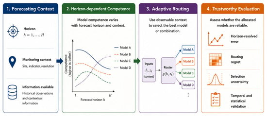
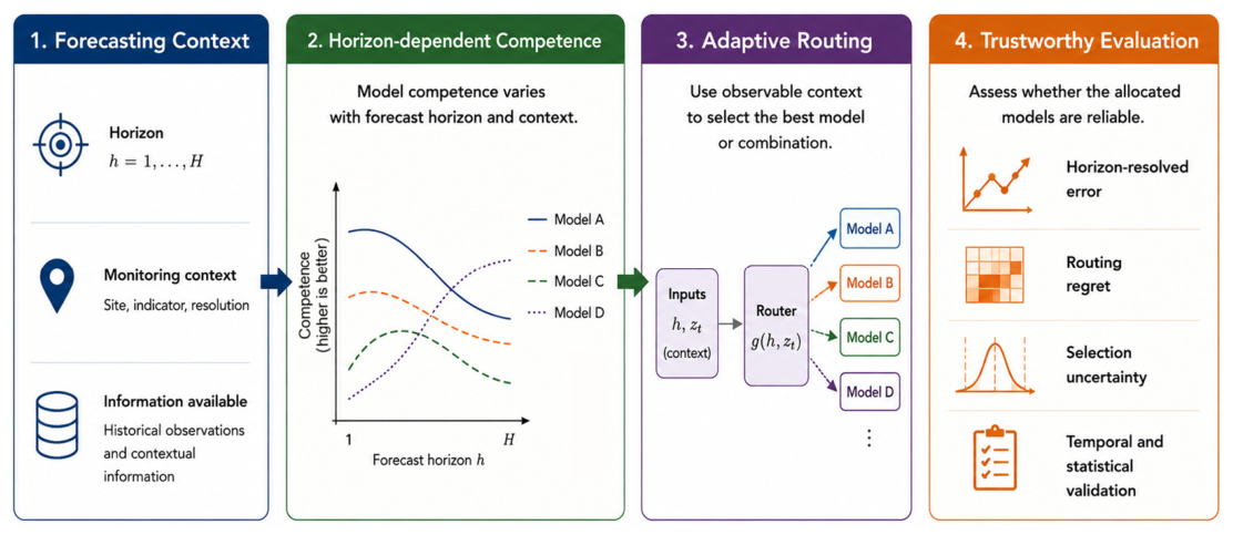
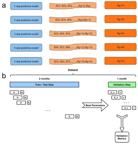
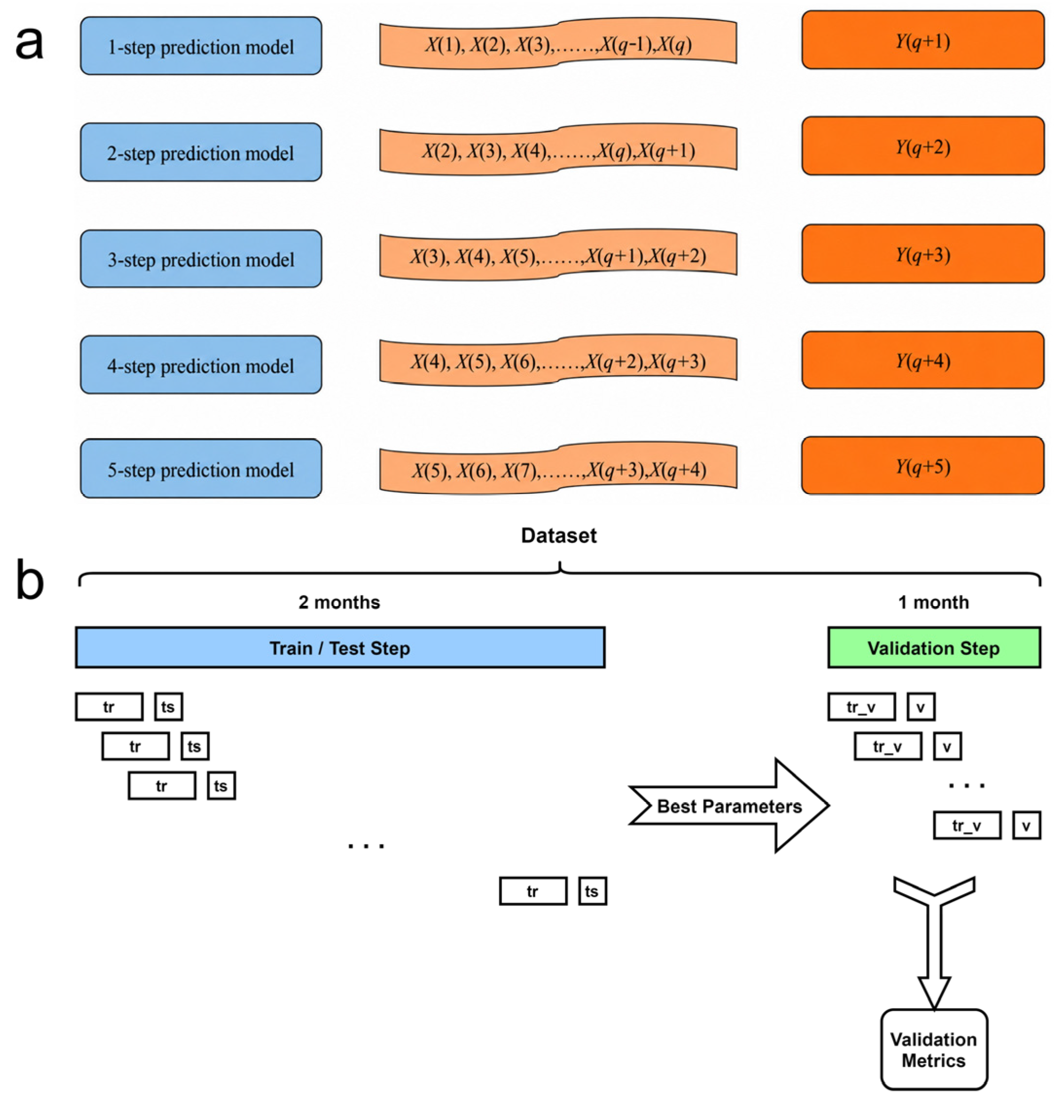
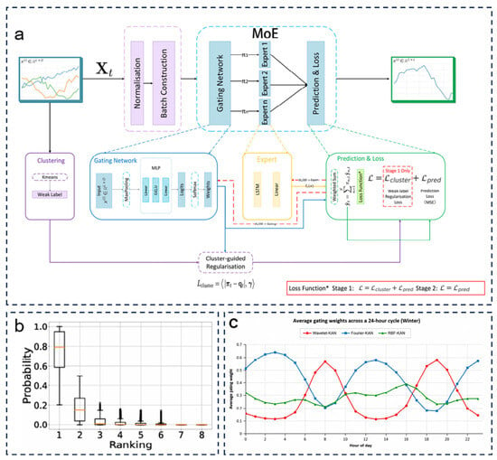
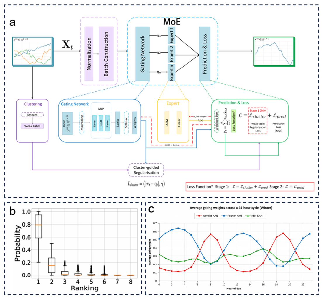
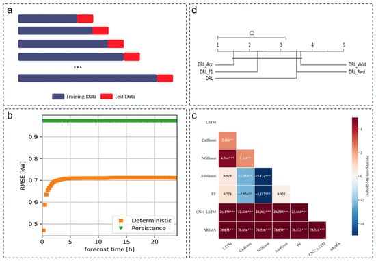
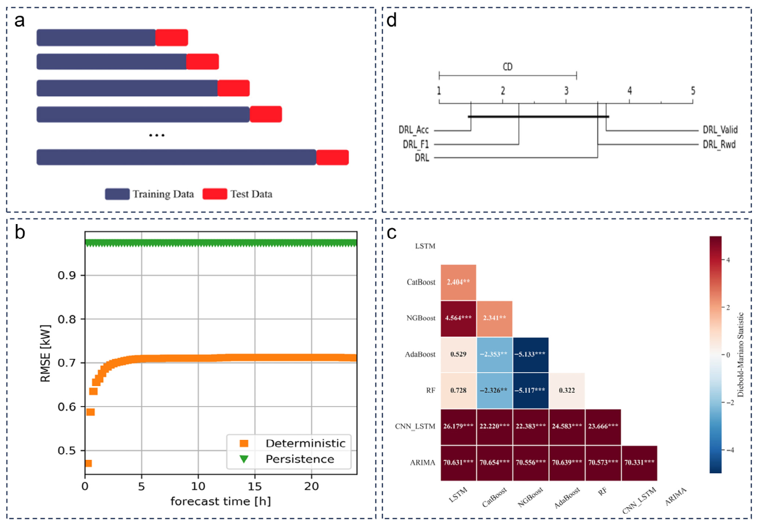

Disclaimer/Publisher’s Note: The statements, opinions and data contained in all publications are solely those of the individual author(s) and contributor(s) and not of MDPI and/or the editor(s). MDPI and/or the editor(s) disclaim responsibility for any injury to people or property resulting from any ideas, methods, instructions or products referred to in the content. |
© 2026 by the authors. Licensee MDPI, Basel, Switzerland. This article is an open access article distributed under the terms and conditions of the Creative Commons Attribution (CC BY) license.