


Abstract
Finite-element analysis (FEA) flux maps are widely used in reduced electrical-machine lookup-table (LUT) models. However, the local dynamics of an implemented LUT representation need not match those inferred from separately interpolated derivative maps. This study develops a representation-aware numerical analysis workflow for a 100 kW externally excited synchronous machine. A formal atlas of 10,230 grid–knot matrices is compared with the audited trilinear representation at grid knots and at 5000 strictly off-grid cell-center equilibria. Although interior-knot constructions agree closely, the Jacobian of the implemented LUT representation is non-Hurwitz at 488 of 5000 within-cell equilibrium centers (9.76%), whereas the derivative-consistent comparator is Hurwitz at all centers. An extended nine-point audit of 1660 center-admissible geometric cells at five speeds (8300 cell-speed groups) retains 73,900 current-limit-valid design locations; within this finite design, 16,526 of 73,900 implemented-model Jacobians (22.36%) are non-Hurwitz, compared with 0% for the derivative-consistent representation. Interpolation-family and grid-resolution sensitivities preserve the qualitative operator-order effect. On the 832-point common strict-domain subset, Heun and classical fourth-order Runge–Kutta (RK4) remain markedly more accurate than Euler-based alternatives. The results show that interpolation–differentiation consistency should be established before interpreting model-predicted local continuous-time stability and fixed-step numerical admissibility. These percentages describe two distinct finite designs and do not estimate continuous-domain prevalence.
Keywords:
electrical-machine lookup tables; finite-element flux maps; interpolation–differentiation mismatch; equilibrium-local Jacobian; Hurwitz classification; cellwise nonsingularity; fixed-step integration MSC:
65L20; 65D25; 65L06
1. Introduction
Modern electrical-machine simulation typically decouples offline finite-element electromagnetic calculations from real-time time-domain system integration. Finite-element analysis is performed offline, and the resulting flux linkage, torque, loss, or inductance data are commonly organized as reusable numerical datasets or lookup tables, then embedded in reduced-order models for controller development, hardware-in-the-loop (HIL) testing, and real-time execution [1,2,3,4,5,6,7,8]. This strategy is particularly useful for nonlinear synchronous machines, including externally excited synchronous machines (EESMs), where saturation, cross-coupling, saliency, and excitation-dependent magnetic behavior can limit the accuracy of constant-parameter models [9,10,11,12,13,14]. Recent studies also examine saliency-dependent dq-current allocation [15] and radial-force harmonics [16], highlighting the broader role of nonlinear electromagnetic effects in machine modeling.
A static magnetic map does not inherently ensure a stable or accurate time trajectory. When precomputed FEA tables are embedded in dynamic differential equations and advanced with a fixed time step, the choice of integration scheme directly determines numerical behavior. Explicit Euler remains attractive in embedded implementations because it requires only one right-hand-side evaluation and no implicit solve, but its absolute stability region is bounded. A locally stable continuous-time electrical model can therefore become unstable under discrete updates if the chosen step moves one or more local modes outside the Euler stability disk. Studies in power-system dynamics and real-time simulation have long shown that numerical stability, damping, and accuracy depend on both the integration scheme and the step size [17,18,19,20,21]. For FEA-informed electrical-machine models, a less-examined question is how the admissible step size varies with the nonlinear magnetic operating point.
This study investigates a specific numerical consistency issue in FEA-informed lookup-table models: whether an independently reconstructed incremental-inductance matrix field remains consistent with the interpolated flux representation between tabulated grid knots. Previous FEA-LUT studies have shown that table construction and interpolation affect dynamic-model fidelity [22,23], but the local consequences of combining these two representations have received less attention. Consistency is assessed using equilibrium-local Jacobians, Hurwitz classification, and fixed-step admissibility. Unlike the neural-correction framework in [24], the present analysis focuses on representation consistency and classical numerical admissibility. The learned correction is examined only after the representation and integration effects have been separated.
The two implementation orders are compared at both grid knots and strictly off-grid locations. The comparison covers off-grid Jacobians, intra-cell tests, interpolation family and grid-resolution sensitivity, and fixed-step solver screening.
Formally, let I denote the interpolation operator applied to the supplied flux-linkage map, Dh the discrete derivative construction used to form the incremental-matrix grid, and D denote differentiation within an interpolation cell. The representation consistency question is whether the independently reconstructed derivative field I(Dhψ) yields the same local differential information as D(Iψ) between tabulated knots. Derivative information from a reconstructed field need not coincide with derivative information reconstructed separately from tabulated data; related consistency and derivative-accuracy issues for interpolated representations have been documented in [25,26]. Accordingly, representation consistency and continuous-time local stability are established before fixed-step solver behavior and the learned corrections are evaluated.
The analysis first assesses whether the differentiated-map construction reproduces the local Jacobian of the audited trilinear flux representation at and between grid knots, and whether any mismatch alters the Hurwitz classification. It then examines the performance of Euler, Heun, and classical fourth-order Runge–Kutta (RK4) when representation consistency and conditional inverter accessibility are accounted for, including a derivative-consistent nonlinear diagnostic based on D(Iψ). The residual-corrected Euler model is considered separately as a secondary stress test under strict-domain selection, spatial separation, training-seed sensitivity, and complete-map Jacobian diagnostics.
Figure 1 summarizes the analysis sequence, from representation consistency and local stability to fixed-step integration and operating-domain assessment.
Figure 1.
Representation-first workflow from FEA maps to off-grid consistency, local stability, fixed-step integration, and operating-domain assessment.
The remainder of the paper follows this hierarchy. Section 2 reviews FEA-informed machine modeling and numerical integration. Section 3 presents the reduced electrical model, grid–knot and strictly off-grid Jacobian audits, conditional voltage masks, classical solver baselines, and secondary correction diagnostics. Section 4 reports representation-consistency and local-stability results, followed by fixed-step solver comparisons and secondary recurrent-map and robustness checks. Section 5 discusses the mathematical interpretation, engineering scope, and limitations, and Section 6 concludes the manuscript.
2. Background and Related Work
FEA-derived surrogate models retain nonlinear electromagnetic information at a fraction of the transient-field cost. Established formulations include finite-element surrogate maps, synchronous-machine flux-array models, spectral interpolation, angle-dependent flux maps, HIL-oriented LUTs, differential-inductance models, and nonlinear synchronous-machine representations [3,4,5,6,7,8,9,10,11,12,13,14]. Kukura et al. [22] showed that LUT construction and interpolation materially affect dynamic accuracy and computational cost, while Mohr et al. [23] identified interpolation error as the residual discrepancy between a LUT-based machine model and its finite-element counterpart. These studies underscore the importance of LUT fidelity. To the best of the author’s knowledge, prior studies have not directly quantified the off-grid discrepancy between I(Dhψ) and D(Iψ) using equilibrium-local Jacobians, Hurwitz-classification changes, and solver-specific fixed-step stability limits.
Numerical integration addresses a complementary question. Early explicit/implicit comparisons in power-system dynamics [17], real-time step-size studies [18], energy-preservation analysis [19], modern Runge–Kutta stability theory [20], synchronous-generator integration studies [21], and related rotating-machine and power-system simulation work [27,28,29] show that an unsuitable discrete update can poorly represent a stable continuous-time model. The unresolved issue for FEA-informed machine models is not whether Euler has a bounded stability region, but rather how the local stability margin varies across a nonlinear magnetic map and how it changes when the practically reachable voltage domain is considered.
Learned dynamical models introduce a recurrent transformation, but that question is secondary here. The generator-corrector framework in [24], stiff neural ordinary differential equation (ODE) studies [30,31], physics-informed approaches [32,33], neural dynamical surrogate models [34,35], and related physics-informed dynamical studies [36,37,38] motivate trajectory- and rollout-level evaluation. Recent studies also address neural differential-algebraic component modeling for electromagnetic-transient simulation [39] and physics-aware surrogate modeling for electromagnetic-loss optimization [40]. Machine-specific neural flux linkage identification [41] provides complementary motivation for evaluating learned electromagnetic representations, whereas spectral normalization [42] and Lipschitz analysis [43] constrain the properties of the neural network mapping. In the present residual-corrected integrator, however, such component-level constraints do not, by themselves, certify the complete numerical time-step map. The learned residual is therefore evaluated only after establishing the FEA-informed representation and classical solver baselines.
Existing literature addresses FEA-LUT interpolation fidelity, numerical differentiation errors, and solver stability as separate topics. Piecewise multilinear reconstructions are only piecewise differentiable, and derivatives computed from an interpolant need not match those reconstructed independently from tabulated data [25,26]. To avoid overly optimistic evaluation under structured spatial dependence, neighboring FEA operating points are not treated as independent experimental units, consistent with leakage-aware validation, structured cross-validation, and cluster-aware resampling principles [44,45,46]. For non-normal systems, eigenvalue movement alone need not quantify transient amplification [47]. Previous numerical-analysis studies further support the representation-consistency analysis undertaken here: Queval and Ohsaki validated N-D LUT machine models against circuit-coupled finite elements [48], while Dell’Accio et al., Bruno and Hoch, and Klein and Berrut documented accuracy, sensitivity, and boundary-related issues in numerical differentiation based on interpolated or approximated data [49,50,51]. Piecewise-defined dynamics require additional care: Tolsma and Barton showed that hidden discontinuities can corrupt standard sensitivity trajectories [52], and Calvo et al. used explicit switching-point location and restart in an adaptive Runge–Kutta solver for piecewise smooth initial-value problems (IVPs) [53]. For FEA-informed LUT models of this type, it is critical to assess whether D(Iψ) and I(Dhψ) remain dynamically equivalent away from tabulated nodes. Because this choice enters the equilibrium-local Jacobian directly, its effect must be established before concluding fixed-step stability.
The study first examines a formal atlas of 10,230 grid–knot matrices and then conducts a separate audit of 5000 strictly off-grid cell-center equilibria using the analytic derivative of the trilinear flux interpolant. The resulting operator mismatch I(Dhψ) − D(Iψ) is then examined via spectral-abscissa changes and Hurwitz flips, followed by a balanced 1000-cell-speed-group stress test and an extended nine-point audit over 1660 center-admissible geometric cells at five speeds (8300 cell-speed groups) (73,900 current-limit-valid points). Continuous-time classification is analyzed separately from fixed-step solver admissibility, and the derivative-consistent nonlinear diagnostic is checked using 10/20/40-substep RK4 and eighth-order Dormand–Prince (DOP853) references. The learned Euler residual is retained only as an additional solver-level sensitivity test. The EESM is therefore a case study for a numerical-analysis framework applicable to nonlinear electrical-machine lookup-table models rather than a source of a machine-specific stability constant.
3. Materials and Methods
3.1. FEA Dataset, Nonlinear Electrical Model and Incremental Matrix
The analysis uses the open 100 kW salient-pole EESM dataset from Bergheim and Jonczyk [2], which was used in a field-programmable gate array (FPGA)-oriented real-time simulation study [1]. The dataset provides three-dimensional flux-linkage and electromagnetic-torque maps, along with iron-loss data indexed by current components and mechanical speed, under a power-invariant reference frame convention. Here, id and iq are the direct- and quadrature-axis stator currents, and if is the field current. Under the power-invariant dq convention used in the source dataset [1,2], the current-limited stator domain used for all sampling and domain-validity decisions is defined by Equation (1).
Equation (2) defines the current and flux-linkage vectors; ψd, ψq, and ψf are the corresponding stator-axis and field flux linkages.
The complete incremental flux-current matrix is defined as the Jacobian of the flux-linkage vector with respect to the current vector [9], as shown in Equation (3).
Second-order finite differences form the primary derivative construction; first-order edge differences and natural cubic-spline derivatives are retained as sensitivity alternatives. Because the stator and field coordinates have markedly different numerical scales, raw matrix condition numbers are supplemented by a dimensionless audit. The primary model retains the observed cross-derivative asymmetry rather than removing it by assumption. A separate post hoc sensitivity case, , is used to rebuild the complete local atlas. This is a model-form stress test, not a substitute for ground truth, because the public data do not provide an energy-based coordinate normalization that would justify exchanging all reported cross-derivatives without qualification. The primary atlas therefore uses derivative grids numerically constructed from the published flux-linkage maps, while the symmetrized case measures how strongly the numerical conclusions depend on that modeling choice.
Finite-difference derivatives are evaluated at the tabulated FEA grid coordinates to construct a discrete incremental-matrix grid. In the reduced-order implementation examined in this study, the flux-linkage tables and the precomputed incremental matrix are interpolated separately. The independently reconstructed matrix is denoted by Linc(i) = I(Dhψ)(i), while DIC(i) = D(Iψ)(i) denotes the derivative of the implemented flux interpolant within a cell. Accordingly, Linc is not recomputed as the derivative of the interpolated flux map at each off-grid state. With I denoting the selected interpolation operator and Dh denoting the discrete derivative-grid construction, the two implementation orders I(Dhψ) and D(Iψ) are evaluated independently; equality between them is not assumed. This implemented model is constructed solely from the published FEA maps for the present numerical analysis and should not be interpreted as a reconstruction of the complete FPGA or HIL implementations associated with the source dataset. The derivative-consistent representation serves as a diagnostic comparator.
Equation (4) defines the dimensionless current/flux scaling used to compare conditioning without allowing the very different magnitudes of the stator and field coordinates to dominate the result. Here, Di = diag(√3Is,rms,max, √3Is,rms,max, If,max) and Dψ = diag(max|ψd|, max|ψq|, max|ψf|), with the flux maxima taken from the supplied FEA tables. No symmetry constraint is imposed on the primary incremental matrix; forced Euclidean symmetrization is retained only as a model-form sensitivity test.
The nonlinear time-domain model uses trilinear interpolation of both the tabulated flux-linkage maps and the precomputed incremental-matrix grid on (id, iq, if). Array-index clipping is retained only as an implementation safeguard for locating interpolation cells and is never interpreted as physically valid extrapolation. Atlas construction records nonfinite or singular incremental matrices as failures and terminates rather than silently omitting them. During time-domain evaluation, domain-contact flags propagate separately from the interpolation safeguard, so reported strict-domain results exclude any trajectory or finite-difference probe that touches or leaves the supplied FEA table.
All normalized state perturbations, neural targets, rollout errors, finite-difference steps, and normalized-map Jacobian diagnostics use the state-scale matrix S = diag(30 A, 30 A, 0.35 A), so ξ = S−1(i − i∗). For a trajectory containing N samples, the reported normalized trajectory error is defined as . These values are numerical weighting scales applied consistently throughout the study, not machine ratings. To make the weighting transparent, component-wise current RMSE values in amperes are also reported for the common strict-domain comparison.
At a fixed mechanical speed, the nonlinear flux-map-based dq electrical model can be written in current-state form, as given in Equation (5).
Here, Rs and Rf are the stator and field resistances, p is the number of pole pairs, and n is mechanical speed in rpm. The electrical-speed-dependent rotational coupling is defined by Equation (6).
For each operating point i∗, the terminal voltage is set to the corresponding equilibrium value u∗ = Ri∗ − Ω(Iψ)(i∗). The third component of u is the effective field-winding voltage in Equation (5); no separate brush/contact voltage-drop term is modeled. The dataset does not include rotor inertia, shaft dynamics, inverter switching, or closed-loop control; therefore, the study concerns the fixed-speed nonlinear electrical subsystem.
For the conditional stator-voltage-feasibility analysis, a two-level voltage-source inverter operating in the linear modulation region is assumed. Under the power-invariant dq scaling used here, the sinusoidal pulse-width modulation (SPWM) and space-vector pulse-width modulation (SVPWM) voltage limits are given by Equation (7).
At Vdc = 400 V, the limits are 244.95 V for SPWM and 282.84 V for SVPWM. These masks are used only as conditional stator-voltage-feasibility tests because the source dataset does not specify the inverter topology or modulation strategy; they do not impose field-excitation supply limits, switching-level reachability, or closed-loop current-control constraints. Results are therefore reported first for the current-limited FEA domain and then for the two conditional voltage-feasible subsets. Table 1 summarizes the principal machine, integration, partition, and normalization settings.
Table 1.
Machine and computational settings. FD: finite differences; RMS: root mean square.
3.2. Representation Consistency and Equilibrium-Local Stability Audits
At a fixed speed, the independently reconstructed incremental matrix Linc = I(Dhψ) is used to construct the formal comparison matrix.
The equilibrium Jacobian of the implemented model follows from differentiation of Equation (5). With u∗ and Ω held fixed, define F(i) = u∗ − Ri + Ω(Iψ)(i). At equilibrium, F(i∗) = 0, so the product-rule term containing the derivative of vanishes. At equilibria strictly inside interpolation cells, the implemented-model and derivative-consistent equilibrium Jacobians are
where the respective inverses must exist. The comparison between AΔ and ARHS evaluates the use of a formal matrix in place of the actual linearization of Equation (5). The derivative-consistent model instead replaces Linc with DIC at every right-hand-side evaluation and provides a separate model comparison. Table 2 and the subsequent matrix-specific results retain these distinctions.
Table 2.
Formal Euler critical-step statistics at 6 A. Pass50 is the percentage of grid knots that pass the formal 50 μs Euler linear-screening criterion.
Cellwise invertibility is assessed by expressing the determinant polynomials det(Linc) and det(DIC) in tensor-product Bernstein form. Nonnegative Bernstein basis functions sum to one [54], so strictly positive coefficients imply a positive determinant throughout the closed cell. Stored nodal values and derivative-grid coefficients are treated as exact dyadic rationals; coefficient conversion and determinant numerators use exact integer arithmetic. The audit covers all 1920 cells intersecting the current-limited domain, including 260 with inadmissible centers. The certificates establish invertibility of the exact interpolants defined by the stored coefficients, but do not account for uncertainty in the original FEA solutions.
Internal knots are assigned to the right-hand cell under a half-open convention, with the last cell used at the upper table boundary. For a continuous tensor-product piecewise-trilinear flux interpolant, each column of an incident one-sided Jacobian at an internal face, edge, or vertex depends only on the approach side in its corresponding coordinate. The incident Jacobians contain all Cartesian combinations of these column choices. By multilinearity, the determinant of any convex combination is a product-weighted convex combination of the incident determinants. Their certified positivity therefore makes every matrix in the Clarke generalized Jacobian nonsingular. This argument uses the Cartesian interpolation structure.
Clarke’s inverse function theorem [55] then provides a local Lipschitz inverse at covered internal points. Writing ϕ = (Iψ)(i) and i = ι(ϕ) for this local inverse, the derivative-consistent model has the local flux-coordinate form
For fixed speed and continuous input, this equation is locally Lipschitz in ϕ and has a unique local solution. The corresponding current trajectory is absolutely continuous and satisfies the cellwise current equation almost everywhere. The statement applies until exit from the inverse neighborhood or the tabulated domain. The Linc-based model is separately locally Lipschitz wherever its continuous matrix field is nonsingular.
The structural contribution to the equilibrium spectra is examined with L = Linc(i∗), D = DIC(i∗), sym(X) = (X + XT)/2, and α(A) = maxjReλj(A). A similarity transformation and the skew-symmetry of Ω give
Positive definiteness of sym(RD−1) is thus a speed-independent sufficient Hurwitz condition. The formal-matrix condition replaces D with L. These conditions are evaluated from the reconstructed matrices; Hurwitz classification alone does not imply their satisfaction.
For the implemented-model Jacobian, write Ω = ωeJ, where J is the matrix in Equation (6) with ωe replaced by one. Then
The bound applies to the nonnegative speeds considered here. Its rotational contribution vanishes when D = L and otherwise depends on mismatch orientation and electrical speed. A negative bRHS certifies a Hurwitz matrix; a nonnegative value is inconclusive. The indicator is also evaluated alongside scalar mismatch for descriptive, in-sample ranking.
For a specified matrix A and fixed step h, the explicit-Euler update matrix of the corresponding linear system is
where I3 is the identity matrix. When every eigenvalue satisfies Reλj < 0, the modal critical steps and Euler threshold are
ME = I3 + hA,
The asymptotically stable linear interior satisfies 0 < h < hcrit. No positive asymptotically stable Euler step is assigned if any eigenvalue has a nonnegative real part. The atlas is a matrix- and method-specific screening map: AΔ defines the formal atlas, while ARHS and Acons define the respective within-cell equilibrium screens.
Heun and classical fourth-order Runge–Kutta (RK4) use RH(z) = 1 + z + z2/2 and RRK4(z) = 1 + z + z2/2 + z3/6 + z4/24. The condition maxj|Rm(hλj)| < 1 is evaluated separately for each matrix family. Nonlinear accuracy, boundedness, and domain retention are assessed through trajectories rather than inferred from this modal condition. The 50 μs macro step is a representative numerical benchmark.
For a diagonalizable reference matrix Ac = VΛV−1 and comparison matrix Ad = Ac + E, the Bauer–Fike theorem [56] places every eigenvalue of Ad within κ2(V)‖E‖2 of an eigenvalue of Ac, where κ2(V) = ‖V‖2‖V−1‖2. Consequently, the sufficient Hurwitz-preservation condition is
α(Ac) + κ2(V)‖E‖2 < 0.
Satisfaction of Equation (12) places all perturbed eigenvalues in the open left half-plane; failure is inconclusive. The comparison uses Ac = Acons and Ad = ARHS.
The operator-order effect can also be illustrated with a two-state polynomial flux map sampled on x, y ∈ {−1, 0, 1} and reconstructed bilinearly in [0, 1]2:
With R = 0.3I2, , and second-order three-point derivative-grid formulas, the two-dimensional analogs of Equation (9) at (x, y) = (0.25, 0.25) have relative operator mismatch 0.2320. Their spectral abscissae are −0.0904 for the derivative-consistent model and +0.07835 for the implemented-order model. This constructed example illustrates a representation effect independently of the EESM data.
At tabulated knots, adjacent trilinear cells can have different slopes. Finite-difference RHS matrices use centered probes when both remain inside the table and boundary-safe one-sided probes otherwise. The nominal normalized perturbation is 10−3, with 3 × 10⁻⁴ and 3 × 10⁻³ as sensitivity levels. Interior field levels and the if = 0 and 10 A boundaries are reported separately. This grid–knot construction check is distinct from the analytic cell-interior audit.
The strictly off-grid audit selects 200 distinct current-limit-valid centers without replacement from each of 25 speed-field-center strata, using fixed initialization. Field-cell centers are if = 1,3,5,7,9 A, and the five speeds are 1000, 3000, 5000, 7000, and 9000 rpm. Each of the 5000 points lies inside a unique cell, where DIC is evaluated analytically from eight corner flux values. Equilibrium voltage is recomputed at each point.
The relative mismatches are δA = ‖ARHS − AΔ‖F/‖ARHS‖F and δD = ‖Linc − DIC‖F/‖DIC‖F. A “Hurwitz flip” denotes disagreement between AΔ and ARHS at the same point. Spearman coefficients describe monotonic association; receiver operating characteristic area under the curve (ROC-AUC) describes in-sample ranking of the non-Hurwitz label.
The extended nine-point design evaluates 1660 center-admissible geometric cells at five speeds, forming 8300 cell-speed groups and 332 groups per speed-field-cell stratum. The balanced design selects 40 groups per stratum, or 1000 groups. Each is evaluated at the center and eight factorial locations with local fractions 0.25 and 0.75. Pointwise current filtering retains 8750 of 9000 balanced locations and 73,900 of 74,700 extended locations. These are finite-design fractions, not continuous-domain prevalence estimates.
A separate spatial audit uses the 27 combinations in {0.05, 0.50, 0.95}3 and pointwise current filtering. The matched comparison contains 1250 cell-speed groups from 922 geometric cells. Near-interface quantities are averaged within each group before groups receive equal weight; all locations remain inside cells. Conditional SPWM/SVPWM masks are applied to the same equilibrium designs. The paired nonlinear comparison uses 30 base points, six per speed and balanced by actual-Jacobian Hurwitz status, selected at evenly spaced mismatch ranks. Two perturbation directions, ±(1, −1, 1), are scaled to 0.15 of the local cell span, giving 60 scenarios.
3.3. Interpolation-Family and Grid-Resolution Sensitivity
Because the primary audit uses a piecewise-trilinear representation, two additional sensitivity tests separate the operator-order conclusion from this specific numerical reconstruction. First, the same sampled off-grid equilibria are re-evaluated using a tensor-product cubic interpolation of both the flux maps and the separately constructed derivative grids. For the smooth interpolant, D(Iψ) is evaluated directly from the interpolation representation, whereas I(Dhψ) is obtained by independently interpolating the discrete derivative grid. The comparison therefore preserves the same two implementation orders while changing the interpolation family.
Second, the id − iq tabulation is systematically coarsened while preserving the original field-current coordinates and outer current domain. The derivative grid is reconstructed independently at each retained resolution, and all current-limit-valid cell centers are re-evaluated. These resolution-dependent results are treated as finite design sensitivity diagnostics rather than estimates of continuous-domain instability prevalence. The retained id − iq grids contain 27 × 25, 14 × 13, and 10 × 9 nodes for coarsening factors 1, 2, and 3, respectively, and the six field-current levels are retained.
3.4. Classical Solver Baselines and Secondary Residual-Correction Stress Test
The analysis first establishes classical numerical baselines. Long-horizon nonlinear reference trajectories use RK4 with ten substeps per 50 μs macro step; twenty-substep trajectories provide a refinement check, and one-step training targets use twenty substeps. Reference-domain contact is monitored at every internal RK4 stage. Training samples whose reference touches the table boundary are excluded. Explicit Euler, Heun, and RK4 are evaluated using the same macro step.
Reference consistency is assessed using matched float32-float64 calculations and an independent DOP853 solve with rtol = 10−10 and component-wise atol = (10−9, 10−9, 10−11). A normalized boundary margin of 0.1 is required; 154 candidates yield 100 complete domain-valid comparisons within the 300-attempt limit. Derivative-consistent references additionally use 10/20/40-substep RK4 and DOP853 with a maximum step of 1.25 μs. An event-aligned check stops at internal interpolation planes and restarts under the same half-open cell convention; outer-table contact terminates a strict reference. A separate linear benchmark compares six methods on 1460 formal AΔ matrices at 20 and 50 μs.
The learned component corrects the Euler transition after the classical baselines have been established.
ΦC(i) = i + hf(i;i∗,n) + Sgθ(z).
Here, f(i;i∗,n) = Linc(i)−1[u∗ − Ri + Ω(Iψ)(i)] is the implemented right-hand side. Standardized state and Euler-increment features, normalized speed, and field-current form z. The three-hidden-layer network uses 96 units per layer, tanh activations, spectral normalization, and output factor β = 0.139516. Training alternates the one-step residual and recursive rollout losses,
Here, B = 128 and H = 4. Training and validation data select the hyperparameters, followed by refitting across eight seeds. The selected settings are λR = 0.3, AdamW learning rate 3.863 × 10⁻³, and weight decay 1.214 × 10⁻⁷. The two losses use alternating updates rather than a single summed backward pass.
3.5. Recurrent-Map Sensitivity Diagnostics
For ξ = S−1(i − i∗), define . At differentiable states, sensitivity of the complete normalized transition is evaluated using the induced Jacobian norm, which equals its maximum singular value. A sampled value below one supplies local differential information. Domain-wide contraction additionally requires a self-map on a suitable domain and a uniform Lipschitz bound below one. Centered differences use a nominal normalized perturbation of 10−3 and an epsilon sweep. The complete derivative includes . Since tanh is 1-Lipschitz, bounds the residual network alone; denotes its linear-layer matrices. This component bound does not bound the complete transition without the Euler and feature derivatives.
For a K-step trajectory segment, the product of local Jacobians quantifies infinitesimal amplification along the evaluated trajectory. The product uses K = 20 steps, or 1 ms at 50 μs. A lower segment gain is assessed separately from a uniform contraction bound for the complete K-step map. The single-step sensitivity and K-step amplification measures are defined as follows:
3.6. Spatially Guarded Evaluation, Two-Way Crossed Resampling and Timing
Neural evaluation uses interior field-current levels of 2, 4, 6, and 8 A. A 5 × 5 current-plane block, split with a 75 A guard, yields 2600/980/1460 training/validation/test points, 1780 guard points, and at least 100 A separation between active partitions; all perturbations from one operating point inherit its partition.
The primary horizon is one electrical period, Te = 60/(pn), corresponding to 30.0–3.33 ms across 1000–9000 rpm. Robust testing uses 14 perturbations per test point (20,440 scenarios), whereas the complete-map Jacobian analysis uses six (8760 scenarios).
Because neighboring FEA operating points are correlated, paired inference uses a two-way crossed bootstrap over training seeds and spatial speed-field-block clusters [46]. For each seed-by-cluster cell, the median paired RMSE difference is computed, and the reported point estimator is the median of these cell-level medians. Training seeds and spatial clusters are independently resampled with replacement using 50,000 bootstrap replicates and five RNG repeats; the 2.5th and 97.5th percentiles are reported as a 95% crossed-bootstrap resampling interval. Eight leave-one-training-seed-out repetitions provide an additional seed-sensitivity check. These intervals are conditional on the observed paired subset and the sampled operating map.
A selection audit compares retained and excluded operating points using local Euler critical step, equilibrium voltage, rollout error, voltage feasibility, and domain-contact rates. Central processing unit (CPU) timing is reported as the mean across 200 repeats for each batch size and method; it is a platform-specific software measurement, not an embedded real-time benchmark. The numerical analyses were performed in Python 3.13.15 using NumPy 2.1.3, Pandas 2.2.3, SciPy 1.16.3, Matplotlib 3.10.0, PyTorch 2.11.0 (CPU), and Optuna 5.0.0.
4. Results
4.1. Representation Consistency, Local Stability and Incremental-Matrix Audit
All 10,230 formal comparison matrices in the grid–knot atlas are Hurwitz; this is an algebraic classification of the matrices rather than a classical nonlinear linearization at nonsmooth knots. At if = 6 A, the median formal explicit-Euler critical step decreases from 2266.93 μs at 1000 rpm to 306.41 μs at 3000 rpm, 113.12 μs at 5000 rpm, 57.98 μs at 7000 rpm, and 35.14 μs at 9000 rpm. The 9000 rpm current-plane range is 22.79–49.50 μs, so no point on that tabulated 6 A grid plane satisfies the 50 μs formal Euler condition. Across the four interior field-current grid levels, formal 50 μs Euler screening coverage is complete through 5000 rpm, approximately 71.6% at 7000 rpm, and 0.29% at 9000 rpm. These are formal grid–knot matrix results; the off-grid audit below determines whether they transfer to the implemented interpolated representation.
The high-speed screening result holds across the tested derivative-construction alternatives. Compared with the second-order finite-difference baseline, cubic-spline derivatives shift the median critical step by 0.88% and alter the 50 μs classification at 0.743% of points; first-order edge treatment yields 0.596% disagreement.
The grid–knot consistency check is very close across the four interior tabulated field-current levels, but its interpretation is deliberately limited. At ε = 10−3, 6820 interior grid knots have a median relative Frobenius difference of 6.75 × 10⁻⁶ and a 95th percentile of 2.75 × 10⁻⁵ between the formal comparison matrix and the symmetric finite-difference right-hand-side linearization. All corresponding finite-difference linearizations are Hurwitz; the median relative Euler critical-step difference is 0.035%, and the 50 μs Euler classification agrees at 99.93% of points. At if = 0 and 10 A, the median matrix difference rises to 19.4%, the finite-difference Hurwitz fraction is 60.4%, and the 50 μs Euler classification agreement is 62.1%. These boundary-safe one-sided RHS differences and the formal atlas use different derivative conventions at potentially nonsmooth knots. The interior result is therefore treated as a grid–knot construction check rather than as proof of off-grid derivative consistency.
The strictly off-grid cell-center audit reveals a representation-induced qualitative stability change that the grid–knot check obscures. Across 5000 sampled cell-center equilibria, the median relative difference between the formal comparison matrix AΔ and the actual within-cell implemented-model Jacobian is 1.80%; the 95th percentile is 13.45%; and the maximum is 34.18%. The overall median is reduced by the two field cells adjacent to if = 0 and 10 A, where the median matrix difference is 0.118%; within the central if = 3, 5, and 7 A cells, the median difference is 6.19%, with a 95th percentile of 16.44%. The formal comparison matrix is Hurwitz at every sampled point, whereas the actual within-cell implemented-model Jacobian is Hurwitz at only 90.24% of samples. For Euler, the 50 μs linear-screening classification agrees at 84.02% of points; the corresponding agreement fractions are 90.22% for Heun and 90.24% for RK4. Thus, for the discrete derivative grid construction and trilinear interpolation used here, I(Dhψ) and D(Iψ) are not interchangeable between knots, and the mismatch can change qualitative continuous-time stability classification rather than merely perturb a fixed-step boundary.
Of the 5000 sampled off-grid equilibria, 488 (9.76%) have a positive spectral abscissa for the actual within-cell implemented-model Jacobian, even though the formal comparison matrix remains Hurwitz. Within this non-Hurwitz subset, the median positive spectral abscissa is 29.60 s−1, the 95th percentile is 90.47 s−1, and the maximum is 126.19 s−1. The classification is not dominated by values arbitrarily close to zero: only 13 points have 0 < α < 1 s−1, 63 have 0 < α < 5 s−1, and 100 have 0 < α < 10 s−1. The non-Hurwitz fraction is higher at 9000 rpm than at 1000 rpm, increasing from 13/1000 to 159/1000 sampled points. These results characterize the local stability of the sampled implemented representation and are specific to the evaluated finite design, rather than constituting evidence of physical machine instability or a continuous-domain prevalence estimate. Each flagged equilibrium lies strictly inside a cell, where the nonsingular implementation is continuously differentiable. A positive-real-part eigenvalue therefore implies local instability of that implemented equilibrium; substituting the formal Hurwitz matrix would miss this classification.
Conditional voltage accessibility does not eliminate the off-grid classification change. Of the 2450 SPWM-feasible sampled cell centers, 179 (7.31%) are non-Hurwitz under the actual within-cell implemented-model Jacobian; for the 2680 SVPWM-feasible centers, 234 (8.73%) are non-Hurwitz. By contrast, the local derivative-consistent baseline formed with D(Iψ) is Hurwitz at all 5000 sampled centers and at every SPWM- and SVPWM-feasible center. D(Iψ) is available and numerically invertible at all 5000 sampled centers in this audit; its raw 2-norm condition number has a median of 1.34 × 10³ and a 95th percentile of 3.51 × 10³. This local comparison shows that the qualitative classification change is associated with the mismatch between the separately interpolated differential matrix and the derivative of the audited flux interpolant within the evaluated numerical representations. The additional nonlinear derivative-consistent integration reported below tests the trajectory-level consequences separately.
The apparently large 19.4% boundary-knot discrepancy at if = 0 and 10 A and the much smaller 0.118% median discrepancy at the adjacent if = 1 and 9 A cell centers are not contradictory. The former uses a boundary-safe finite-difference convention at a grid–knot where the piecewise-trilinear map need not have a unique classical derivative, whereas the latter uses the analytic derivative strictly inside the adjacent interpolation cells. They therefore quantify different derivative conventions at different locations.
Independent reference-integration checks quantify the numerical consistency of the implemented model’s high-resolution RK4 baseline. The 10- versus 20-substep RK4 comparison yields a median normalized difference of 1.71 × 10⁻⁶, a 95th percentile of 5.51 × 10⁻⁶, and a maximum of 1.64 × 10⁻⁵. Across 200 matched samples, float32 and float64 ten-substep references differ by a median normalized RMSE of 1.27 × 10⁻⁶, a 95th percentile of 4.10 × 10⁻⁶, and a maximum of 5.80 × 10⁻⁶. The adaptive DOP853 audit reaches its target of 100 full-horizon domain-valid comparisons after 154 candidate attempts. For those 100 cases, the ten-substep RK4 reference differs from DOP853 by a median normalized RMSE of 1.57 × 10⁻⁸, a 95th percentile of 2.2 × 10⁻⁵, and a maximum of 5.1 × 10⁻⁵; the twenty-substep comparison yields 1.34 × 10⁻⁸, 1.2 × 10⁻⁵, and 2.9 × 10⁻⁵, respectively. These checks support numerical consistency for the evaluated domain-valid trajectories; they do not constitute transient-FEA or experimental validation.
All sampled incremental matrices are nonsingular, and the cellwise determinant certificates cover all relevant interpolation cells. The large raw 2-norm condition number (median 1406.7) is partly due to the differing scales of the stator and field coordinates. The dimensionless audit yields a median condition number of 24.59, a 95th percentile of 54.75, and a maximum of 57.10. Across the 1364 unique current-field points, the smallest raw singular value is 6.77 × 10⁻⁵ H. The median relative Frobenius asymmetry is 12.19% (95th percentile 12.98%), treated as a model-form sensitivity rather than dismissed as a negligible numerical residue.
The forced-symmetry stress test substantially alters the model. Although a symmetric matrix can be formed at every point, only 37.93% of the resulting 10,230 formal comparison matrices remain Hurwitz, and the 50 μs classification disagrees with the unsymmetrized formal-matrix baseline at 50.69% of points. On the Hurwitz subset of the symmetrized formal matrices, the median relative change in critical step is +17.47%, while the 95th-percentile absolute change reaches 137%. At 9000 rpm and 6 A, only 32.84% of the symmetrized formal matrices are Hurwitz; among these, the median critical step is 57.26 μs, and 26.98% of the complete current plane passes the formal 50 μs Euler screen. At the same 9000 rpm and 6 A operating plane, all unsymmetrized formal matrices are Hurwitz, but none passes the formal 50 μs Euler screen. These results show that a posteriori Euclidean symmetrization should not substitute for an energy-consistent constitutive reconstruction. Because the public flux maps do not uniquely determine a scalar co-energy representation or a corresponding regularization strategy, no energy-consistent ground-truth model is imposed in the present study. Constructing such a representation would require a separate model-identification step and is therefore outside the scope of this representation-order audit.
Figure 2 summarizes the formal grid–knot screening and the actual off-grid Jacobian results. Figure 2a presents the formal Euler critical-step distribution at 9000 rpm and 6 A, while Figure 2b shows that the overall trend is only weakly affected by the derivative construction. Figure 2c presents the off-grid spectral abscissa distribution, and Figure 2d compares the Euler critical steps at operating points where both matrix families are Hurwitz. Table 2 further shows that, at if = 6 A, the median formal Euler critical step decreases from 2266.93 μs at 1000 rpm to 35.14 μs at 9000 rpm, with a maximum of 49.50 μs at the highest speed; thus, none of the grid knots on this 6 A plane satisfies the formal 50 μs Euler linear-screening criterion at 9000 rpm.
Figure 2.
Formal grid–knot screening and off-grid Jacobian comparison. (a) Formal Euler critical step at 9000 rpm and 6 A. (b) Derivative-construction sensitivity. (c) Actual off-grid spectral abscissa; dashed line: α = 0. (d) Euler critical steps where both matrices are Hurwitz.
Exact Bernstein calculations establish positive determinants for Linc and DIC across all 1920 relevant cells. A Routh-Hurwitz check agrees with the direct eigenvalue classification of the implemented-model Jacobian at all 5000 centers. No attracting or repelling case is observed among the 204,300 sampled interface-direction configurations. These finite-direction checks complement the interpolation-specific local inverse argument rather than providing a uniqueness proof (Table 3).
Table 3.
Cellwise invertibility and additional checks. The scopes of determinant certificates, sampled interface directions, and trajectory calculations are distinct.
The constructed analytic map reproduces the same qualitative operator-order mechanism without using EESM data. At the reported point, the relative mismatch is 0.2320, and the spectral abscissa shifts from −0.0904 for the derivative-consistent model to +0.07835 for the implemented-order model. The numerical midpoint-grid classification-difference fraction changes from 41.27% at 21 × 21 to 41.41% at 161 × 161, with successive changes below 0.08 percentage points beyond the coarsest grid. This example illustrates the non-commutation mechanism but does not provide physical validation of the machine model.
The operator-mismatch analysis shows that Hurwitz flips are associated with larger representation mismatch, but not in a simple monotonic relationship. Across the 5000 cell centers, the median normalized derivative operator mismatch is 0.02947 for the 488 flip points and 0.01050 for the 4512 non-flip points. The Spearman coefficients are −0.062 for mismatch versus implemented-model spectral abscissa and −0.154 for mismatch versus implemented-minus-consistent spectral abscissa shift. The Bauer–Fike sufficient condition did not certify any sampled point; the conservative eigenvector-conditioning-dependent bounds do not imply instability.
Neither the derivative-consistent positive-definiteness condition nor its formal-matrix counterpart certifies any sampled center, even though both the derivative-consistent and formal comparison matrices are Hurwitz according to direct eigenvalue classification. The structured RHS bound also certifies no center. Its Spearman correlation with α(ARHS) is 0.2313, compared with −0.0623 for δD. The pooled in-sample ROC-AUC values are 0.8903 for the structured indicator and 0.5657 for relative operator mismatch, but the structured-indicator AUC is 0.3625 at 1000 rpm (Table 4). The indicator provides a stronger pooled ranking within this design without establishing a generally successful prediction rule.
Table 4.
In-sample structural-indicator discrimination and sufficient-condition outcomes at 5000 centers.
Applying the same dimensionless current/flux scaling to both representations shows that the off-grid classification difference is not due to a gross conditioning mismatch. Across all 5000 centers, the median and P95 scaled 2-norm condition numbers are 25.99/53.41 for D(Iψ) and 25.91/52.53 for I(Dhψ); at the 488 Hurwitz-flip points, the corresponding medians are 41.66 and 41.63. The median pointwise ratio is 0.9988.
The balanced 1000-cell-speed-group robustness test retains 8750 of 9000 requested center-plus-factorial points because the circular current limit removes 250 strict-interior offsets near the domain boundary. Among these 8750 retained points, 1859 implemented-model Jacobians are non-Hurwitz (21.25%), and all 105 center-non-Hurwitz cell-speed groups retain at least one non-Hurwitz off-center point. The extended nine-point audit covers 1660 center-admissible geometric cells at five speeds (8300 cell-speed groups) and retains 73,900 of 74,700 requested design points after pointwise current-limit filtering. Within this finite design, 16,526 audited-representation Jacobians are non-Hurwitz (22.36%), whereas the derivative-consistent representation shows no non-Hurwitz Jacobians. A total of 62.43% of cell-speed groups contain at least one flagged valid point; the equal-group-weighted mean non-Hurwitz fraction is 22.31%, and all 826 center-non-Hurwitz cell-speed groups retain an off-center non-Hurwitz point. The close point-weighted and equal-cell-weighted fractions indicate that unequal retention among the evaluated center-admissible cell-speed groups does not dominate the reported result; these finite-design fractions are not continuous-domain prevalence estimates.
In the matched spatial audit, the center non-Hurwitz fraction is 9.84%, and the equal-group-weighted near-interface fraction is 30.36%, a difference of 20.52 percentage points. The locations remain within interpolation cells. The comparison establishes location sensitivity within this finite design without implying a causal discontinuity mechanism.
The interpolation-family and grid-resolution sensitivity analyses preserve the qualitative operator-order conclusion while showing that its magnitude depends on the numerical representation. At the same 5000 off-grid centers, the tensor-product cubic reconstruction yields 537 non-Hurwitz cases (10.74%) for the implemented representation, whereas the derivative-consistent representation remains Hurwitz at all 5000 centers; the corresponding primary trilinear result is 488/5000 (9.76%). In the complete cell-center grid-resolution audit, the non-Hurwitz fractions for the separately interpolated representation are 9.95%, 22.93%, and 44.22% for coarsening factors 1, 2, and 3, respectively, while the derivative-consistent representation remains at 0% for all three resolutions. These results indicate that the qualitative operator-order effect persists across the tested interpolation and grid-resolution choices, whereas its quantitative extent is resolution-dependent. The 9.76% trilinear result is based on 5000 sampled off-grid centers, whereas the 9.95% coarsening factor-1 result includes all current-limit-valid cell centers at that resolution.
For the retained strict-domain cases, the nonlinear derivative-consistent diagnostic shows that changing the representation alters the simulated vector field rather than acting as a simple solver correction. Across 60 scenarios, 27 Euler pairs and 29 Heun/RK4 pairs remain strict in both representations over one electrical period. For those strict pairs, the median high-resolution cross-representation trajectory difference is 0.235 for Euler and 0.237 for Heun/RK4. At the common 50 μs macro step, derivative consistency lowers solver error relative to its own high-resolution reference in 37.0% of Euler, 10.3% of Heun, and 6.9% of RK4 pairs. The median derivative-consistent RMSE is 0.1020, 0.01422, and 0.01449 for Euler, Heun, and RK4, respectively, compared with 0.07550, 0.001062, and 8.16 × 10⁻⁶ for the implemented representation. The derivative-consistent reformulation therefore changes both the continuous model and its numerical difficulty and should not be interpreted as a universally accuracy-improving solver correction.
The stratified audit makes the retained sample size and selection effect explicit. Euler’s strict-pair counts at 1000/3000/5000/7000/9000 rpm are 8/7/2/5/5 out of 12 scenarios per speed; Heun and RK4 retain 8/7/3/5/6. Across the intentionally balanced Hurwitz strata, Euler retains only 3/30 scenarios from implemented-model-non-Hurwitz bases versus 24/30 from implemented-model-Hurwitz bases; Heun and RK4 retain 4/30 versus 25/30. None of the retained non-Hurwitz-base scenarios favors the derivative-consistent model at 50 μs. The nonlinear comparison is therefore treated as a diagnostic of representation change, not as an unbiased frequency estimate over the operating domain.
The boundary-aware reference audit provides an additional numerical qualification. Across all 60 derivative-consistent scenarios, the median 10-substep-versus-40-substep RK4 difference is 0.00273 normalized RMSE (P95 0.0943), while the primary 20-substep-versus-40-substep difference is 0.00213 (P95 0.0520). Thirty-three scenarios remain strict for both the 40-substep RK4 and DOP853 references; their median RK4-versus-DOP853 difference is 2.17 × 10⁻⁴, with P95 0.00825 and a maximum of 0.0147. The high-resolution derivative-consistent trajectories cross a median of seven interpolation cell interfaces. Together, the DOP853 and event-aligned audits support numerical consistency for the evaluated strict-domain trajectory comparisons, with explicit interpolation-interface handling assessed separately in the event-aligned audit. A separate event-aligned audit was performed on 30 derivative-consistent scenarios, of which 20 remained strict and directly comparable with the 40-substep RK4 reference. The median normalized RK4-40/event-aligned difference is 1.43 × 10⁻⁴ (P95 0.00241; maximum 0.002448), with a median of five explicitly resolved interpolation interface events.
Figure 3 summarizes the principal representation diagnostics. Figure 3a indicates that the magnitude of the operator mismatch alone does not monotonically predict the spectral abscissa, whereas Figure 3b shows that non-Hurwitz classifications persist at off-center locations within the balanced cell-speed sample. Figure 3c shows that switching to the derivative-consistent representation does not systematically reduce fixed-step error, while Figure 3d shows that the two representations have closely matched dimensionless conditioning. The extended nine-point cell-speed audit complements the sampled distribution in Figure 3b by showing that the observed off-center persistence is not confined to the balanced subset.
Figure 3.
Representation diagnostics. (a) Operator mismatch versus the actual spectral abscissa. (b) Off-center non-Hurwitz persistence in the balanced cell-speed design. (c) Representation-specific nonlinear solver errors. (d) Dimensionless conditioning.
4.2. Conditional Voltage-Feasible Domain
The dc-link sensitivity alters the interpretation of the high-speed current map but not the formal linear-screening conclusion. At 9000 rpm and if = 6 A, the 341-point current-limited domain requires equilibrium voltage magnitudes well beyond the 400 V two-level linear modulation capability. Under the power-invariant SPWM convention, only 17 points (4.99%) remain; under SVPWM, 25 points (7.33%) remain. Every retained formal matrix still has hcrit < 50 μs. At 7000 rpm, the retained fractions are 8.80% and 13.49%, respectively, and none of the retained 6 A points satisfy the formal 50 μs linear-screening condition. At 5000 rpm, the feasible subsets are larger—26.98% for SPWM and 44.57% for SVPWM—and all retained points satisfy the formal 50 μs linear-screening condition.
Because the inverter topology and modulation are not specified in the public data, these masks are sensitivity conventions rather than assertions about the original test bench. They do, however, show that the term conditional voltage-feasible equilibrium subset must be used carefully: the current-limited FEA grid and the conditional voltage-feasible equilibrium subset are not identical.
Figure 4 illustrates the distinction between the current-limited FEA domain and the voltage-feasible domain at 9000 rpm. Table 5 extends this comparison to 5000–9000 rpm and shows that the conditional voltage constraints substantially reduce the retained operating set as speed increases. At 7000 and 9000 rpm, none of the operating points retained under either the SPWM or SVPWM convention satisfy the formal 50 μs Euler linear-screening criterion.
Figure 4.
Equilibrium stator-voltage demand at 9000 rpm and 6 A under conditional two-level SPWM/SVPWM limits. The dotted black contour denotes the stator-current limit, while the inner and outer voltage-limit contours correspond to the SPWM and SVPWM limits, respectively.
Table 5.
Conditional voltage filtering of the formal 6 A atlas. Entries are retained count (%); median critical step (μs); pass at 50 μs (%).
The same conditional masks applied to the actual off-grid Jacobian audit show that the non-Hurwitz classification persists within voltage-feasible subsets. Across all speeds, 179 of 2450 SPWM-feasible sampled centers (7.31%) and 234 of 2680 SVPWM-feasible sampled centers (8.73%) have positive implemented-model within-cell spectral abscissa. The effect remains nonzero in the high-speed feasible subsets: at 7000 rpm, 22/91 SPWM-feasible and 39/149 SVPWM-feasible sampled centers are non-Hurwitz; at 9000 rpm, the corresponding counts are 8/55 and 20/86. These fractions are conditional on the adopted two-level linear-modulation conventions and the cell-center sampling design; they should not be interpreted as switching-level reachability guarantees or continuous-domain prevalence estimates. The corresponding excluded-set non-Hurwitz counts are 309 of 2550 (12.12%) for SPWM and 254 of 2320 (10.95%) for SVPWM. Median operator mismatch is larger inside the masks: 1.446% versus 1.101% for SPWM and 1.510% versus 1.043% for SVPWM.
The speed-stratified comparison further resolves this pattern. At 5000 rpm, SPWM-feasible centers contain 75 flagged points among 304 (24.67%), compared with 39 among 696 excluded centers (5.60%). The lower pooled inside fraction therefore does not imply a lower fraction at every speed (Table 6). These conditional equilibrium masks do not establish switching-level reachability.
Table 6.
Actual off-grid non-Hurwitz fractions inside and outside conditional voltage masks.
4.3. Classical Solver Performance and Secondary Residual-Correction Audit
Across all 1460 test points, the median normalized one-period RMSE is 0.2711 for Euler and 0.2713 for corrected Euler. On the common 832-point strict-domain subset, the medians are 0.13867, 0.12646, 0.001722, and 3.375 × 10⁻⁵ for Euler, corrected Euler, Heun, and RK4. Corrected Euler improves at 469 of 832 points (56.37%). Heun and RK4 remain substantially more accurate (Figure 5).
Figure 5.
One-period nonlinear solver errors. (a) Held-out error distribution. (b) Speed-stratified errors on the selected 832-point common strict-domain subset. The paired numerical claims in the text concern the strict subset. (Orange horizontal lines in panel (a) denote median values).
The aggregate correction benefit increases with speed: improvement fractions are 0% at 1000 rpm, 22.54% at 3000 rpm, 91.08% at 5000 rpm, and 100% at 7000 and 9000 rpm. Of the 469 improved points, 430 occur at speeds of at least 5000 rpm. The paired seed-by-cluster estimator is −0.04737 for corrected minus Euler, with a recorded 95% crossed-bootstrap resampling interval of [−0.08374, −0.0008665]. Five of eight seed-omission intervals include zero.
Supplementary Figure S1 presents the spatially guarded training partition and comparisons of residual-network Jacobian norms. The network-only norms do not certify contraction of the full time-step map.
The retained points have a median formal Euler critical step of 147.8 μs, compared with 73.9 μs for 628 excluded points; the median Euler RMSE is 0.139 versus 1.046. Corrected Euler improves at 9.90% of 394 SPWM-feasible and 12.71% of 409 SVPWM-feasible common-strict points. Its benefit is therefore conditional on selection and voltage filtering. Component-wise current RMSE in amperes, ordered (d, q, f), is (3.145, 0.877, 0.0764) for Euler, (2.808, 0.908, 0.0678) for corrected Euler, (0.0413, 0.0146, 0.000922) for Heun, and (0.000725, 0.000302, 0.0000182) for RK4.
Table 7 shows a clear speed-dependent change in the relative performance of Euler and corrected Euler. The correction is less effective at 1000 and 3000 rpm but becomes advantageous at 5000 rpm and above. Even so, Heun and RK4 maintain substantially lower errors across the entire speed range.
Table 7.
One-period normalized RMSE on the 832-point common strict-domain subset.
4.4. Secondary Recurrent-Map Sensitivity and Finite-Time Diagnostics
Across 8760 instantaneous probes, the spectral radius is at least one in 48.37% of Euler and 38.24% of corrected-Euler scenarios; the maximum singular value is at least one in every case. For 8618 paired strict-domain 1 ms products, the median gains are 7.445 and 7.230. Corrected Euler has a lower product gain in 63.62% of cases, but every product norm exceeds one. These sampled local and finite-time diagnostics do not provide a domain-wide contraction certificate.
The corresponding instantaneous sensitivity distributions and the full finite-time summary are provided in Supplementary Figure S2 and Supplementary Table S1, while the paired 20-step product gains are shown in Supplementary Figure S3.
Contact with cells whose centers have non-Hurwitz Jacobians occurs in 24.5%, 25.4%, and 27.3% of reference, Euler, and corrected trajectories, respectively. On the common strict subset, the corresponding fractions are 7.1%, 7.9%, and 8.8%. This diagnostic identifies entry into cells with flagged centers; the center label does not classify every state within the cell.
4.5. Fixed-Step Coverage, Robustness and Timing
On the same 1460 formal AΔ systems, Euler passes at 73.63% of points for 50 μs and at 100% for 20 μs. Its median relative matrix-propagator error decreases from 0.03738 to 0.00873. Heun, RK4, backward Euler, and the trapezoidal rule pass at all points at both steps, although their errors differ substantially (Table 8). These formal linear-system results are distinct from the nonlinear and actual off-grid comparisons. The corresponding 95th-percentile relative matrix-propagator errors at 50 μs are reported in Supplementary Table S2.
Table 8.
Matched 20 and 50 μs benchmark on 1460 formal matrices. Errors are relative matrix-propagator errors.
The formal grid–knot Euler screening coverage curve is a screening result only: at 50 μs, it is 100% through 5000 rpm, ≈71.6% at 7000 rpm, and 0.29% at 9000 rpm; 20 μs restores 100% coverage at the sampled knots. Inconsistent off-grid representation prevents treating these values as guarantees of the implemented model.
Across all six field-current grid levels at 9000 rpm, the median formal grid–knot hcrit values are 35.32/364.34/1534.72 μs for Euler/Heun/RK4; the corresponding formal 50 μs screening coverage is 0.49% for Euler and 100% for Heun and RK4. This all-level summary is distinct from the four-interior-level coverage reported above and remains a grid–knot screening result rather than an analytic off-grid guarantee. Figure 6 shows the formal grid–knot screening coverage across the tested step sizes.
Figure 6.
Formal grid–knot Euler screening coverage versus speed and step size. Reducing the step enlarges the retained formal linear-screening set.
Leave-one-speed-out transfer is descriptive because one seed is used per held speed; corrected-Euler benefit ranges from 0% to 99% across speeds. Mean batch-1 CPU step times are 0.899/1.438/1.843/3.625 ms for Euler/corrected Euler/Heun/RK4; at batch 256, the corresponding mean per-state times are 4.47/8.59/9.08/18.39 μs. These are software-platform measurements, not HIL benchmarks.
Table 8 highlights the distinction between formal linear stability and matrix-propagator accuracy. Although all methods except Euler pass the formal 50 μs linear screen, their approximation errors differ markedly. RK4 yields the lowest nonzero error, followed by the trapezoidal rule and Heun, whereas backward Euler remains stable but offers only limited accuracy improvement relative to Euler.
Table 9 summarizes the key robustness checks conducted throughout the study. The operator-order effect persists under off-grid evaluation, alternative interpolation, grid coarsening, and independent numerical-reference checks. However, the magnitude of the effect remains sensitive to the chosen representation, and the benefit of the learned correction is modest and varies across training seeds.
Table 9.
Consolidated representation, domain, solver, and robustness audit.
5. Discussion
The results show that the separately interpolated derivative map and the derivative of the implemented trilinear flux interpolant are not interchangeable between tabulated knots. At the 5000 sampled centers, ARHS is non-Hurwitz at 488 points, whereas Acons remains Hurwitz throughout. The extended nine-point parent-cell audit strengthens this representation-level result: among 1660 center-admissible geometric cells at five speeds (8300 cell-speed groups), 16,526 of 73,900 retained center-plus-factorial design points (22.36%) are non-Hurwitz in the implemented representation, whereas none are non-Hurwitz in the derivative-consistent representation; 62.43% of the evaluated cell-speed groups contain at least one flagged point, and all 826 center-non-Hurwitz cell-speed groups retain an off-center flagged point. The nearly identical point-weighted (22.36%) and equal-group-weighted (22.31%) fractions indicate that unequal point retention among the evaluated center-admissible cell-speed groups does not explain the observed classification difference. The formal comparison matrix is Hurwitz at every sampled center, so substituting it for the actual Jacobian changes the classification of the same implemented model. The derivative-consistent representation is a separate comparator.
Additional audits of interpolation families and grid resolutions clarify the scope of this result. Under tensor-product cubic interpolation, the non-Hurwitz fraction of the separately interpolated representation is 10.74%, compared with 9.76% for the primary trilinear sample. The derivative-consistent representation remains Hurwitz throughout both 5000-point audits. Controlled grid coarsening increases the separately interpolated cell-center fraction from 9.95% to 22.93% and 44.22%, whereas the derivative-consistent fraction remains zero. The mechanism therefore persists across the tested representations, although its quantitative incidence depends on tabulation density.
Representation mismatch is associated with qualitative stability changes, but the magnitude of the mismatch alone is not a reliable scalar predictor. Hurwitz-flip points have a larger median normalized operator mismatch than non-flip points (0.0295 versus 0.0105), yet rank correlations with the spectral abscissa and its shift are weak. The Bauer–Fike sufficient perturbation check certifies none of the 5000 sampled centers because eigenvector conditioning renders the bound conservative. In contrast, dimensionless matrix conditioning is nearly identical between D(Iψ) and I(Dhψ) (overall medians 25.99 and 25.91), indicating that the classification difference is not a trivial consequence of one representation being globally ill-conditioned. The structured indicator improves pooled in-sample ROC-AUC from 0.5657 to 0.8903, but neither it nor the positive-definiteness conditions certify any sampled center. The sufficient structural conditions therefore cannot, by themselves, explain the observed zero non-Hurwitz counts.
The derivative-consistent nonlinear diagnostic is interpreted as a representation-level trajectory comparison. Across 33 strict pairs, the original small-step DOP853 cross-check remains close to the 40-substep RK4 reference, with a median difference of 2.17 × 10⁻⁴ (P95 0.00825). The additional event-aligned audit yields a median RK4-40/reference difference of 1.43 × 10⁻⁴ (P95 0.00241) across 20 strict, comparable scenarios, with a median of five explicitly resolved interface events [52,53]. For the evaluated strict-domain scenarios, these results suggest that interpolation-interface handling is not the primary source of the observed cross-representation trajectory differences. Nevertheless, the strong attrition of implemented-model non-Hurwitz bases in the strict domain means that this experiment remains a controlled diagnostic rather than an unbiased operating-domain frequency estimate or physical ground truth.
On the 832-point common strict-domain subset, Heun and RK4 remain substantially more accurate than Euler and residual-corrected Euler. The benefit of residual-corrected Euler is comparatively small, seed-sensitive, and substantially reduced within the conditional voltage-feasible subsets. The complete-map and finite-time Jacobian analyses also provide no evidence of normalized 2-norm contraction of the corrected transition. These results support treating the learned residual as a secondary numerical experiment rather than the main contribution of the study. Across all 1460 test points, corrected Euler has no median accuracy advantage over Euler (0.2713 versus 0.2711).
The engineering interpretation is limited to the reduced electrical subsystem represented by the available steady-state FEA maps. The source consists of steady-state FEA maps, rather than transient field solutions or experimental trajectories, and the conditional SPWM/SVPWM masks are equilibrium-accessibility conventions rather than switching-level simulations. The cross-derivative asymmetry and strong forced-symmetry sensitivity also indicate that post hoc model-form corrections are not innocuous. Importantly, derivative consistency with a selected interpolant establishes representation consistency, not electromagnetic reciprocity or energy consistency. Physical validation of either property would require an independently justified constitutive reconstruction or transient field/experimental evidence. Consequently, non-Hurwitz classifications are properties of the implemented reduced representation and must not be reported as evidence of physical EESM instability. The present sensitivity study addresses interpolation, differentiation, tabulation resolution, and numerical integration, but does not quantify uncertainty in the underlying FEA flux-linkage values; consequently, all reported stability classifications are conditional on the supplied FEA maps.
Taken together, the results indicate that the derivative of the implemented interpolant should be checked away from grid knots before interpreting local stability and fixed-step admissibility. The broader contribution is therefore the separation of representation effects from integration effects, rather than the specific instability fractions obtained in this EESM case study.
6. Conclusions
This study examined how representation consistency affects local stability and fixed-step numerical behavior in an FEA-informed lookup-table model of an externally excited synchronous machine. The main finding is that I(Dhψ) and D(Iψ) can yield different local dynamics between lookup-table knots. At 5000 sampled cell centers, 488 actual implemented-model Jacobians are non-Hurwitz, whereas the derivative-consistent baseline is Hurwitz at all centers. The extended nine-point audit evaluates 1660 center-admissible geometric cells at five speeds (8300 cell-speed groups) and retains 73,900 current-limit-valid design locations. Within this finite design, 22.36% of the implemented-model Jacobians are non-Hurwitz, whereas no non-Hurwitz Jacobians are observed under the derivative-consistent representation; moreover, every one of the 826 center-non-Hurwitz cell-speed groups retains at least one off-center non-Hurwitz point. The qualitative classification difference also persists under tensor-product cubic interpolation (10.74% versus 0% derivative-consistent) and under controlled grid coarsening; however, the separately interpolated cell-center non-Hurwitz fraction increases from 9.95% to 22.93% and 44.22% as the grid coarsens, showing that the quantitative extent of the effect is resolution-dependent. These classifications characterize the implemented reduced electrical representation and do not constitute evidence of physical EESM instability. The formal comparison matrix is Hurwitz at every sampled center and therefore cannot replace the actual equilibrium Jacobian in this classification.
The magnitude of operator mismatch helps identify risk but is not, by itself, a stability certificate. Hurwitz-flip points have a median normalized mismatch of 0.0295, compared with 0.0105 for non-flip points, whereas rank correlations with the spectral abscissa are weak. A Bauer–Fike sufficient Hurwitz-preservation test is conservative and inconclusive at all sampled EESM centers. A separately constructed two-state example independently demonstrates that the two operator orders can change Hurwitz classification, while matched dimensionless conditioning of D(Iψ) and I(Dhψ) shows that the observed EESM effect is not explained by a gross conditioning imbalance. Exact cellwise determinant certificates establish nonsingularity of both numerical matrix fields in all 1920 cells intersecting the current-limited domain. The structured spectral bound provides stronger pooled ranking, while its sufficient Hurwitz condition remains inconclusive at every sampled center.
Derivative-consistent re-integration supports distinguishing between a representation change and a solver correction. The original RK4-40/DOP853 cross-check yields a median difference of 2.17 × 10⁻⁴ across 33 strict pairs, whereas the event-aligned audit yields a median difference of 1.43 × 10⁻⁴ (P95 0.00241) across 20 strict comparable scenarios. For the implemented model, the 832-point common strict-domain comparison still favors higher-order classical methods, with median normalized RMSE 0.1387/0.1265/0.001722/3.4 × 10−5 for Euler/corrected Euler/Heun/RK4. This selected-subset comparison does not establish a full-set advantage for corrected Euler, whose median RMSE over all 1460 points is 0.2713 versus 0.2711 for Euler.
More generally, the results suggest establishing representation consistency before interpreting fixed-step solver behavior, particularly when derivative information is reconstructed separately from the interpolated state-dependent map. The case study shows that a grid–knot derivative audit alone is insufficient for a lookup-table model whose off-grid dynamics depend on a separately reconstructed derivative representation. Interpolation-family, tabulation-resolution, and interface-handling sensitivities further define the numerical scope for interpreting the resulting local-stability classifications. A grid–knot derivative atlas should therefore not be interpreted as an off-grid guarantee unless the interpolation-derivative convention has been explicitly audited.
Supplementary Materials
The following supporting information can be downloaded at https://www.mdpi.com/article/10.3390/math14213880/s1: Figure S1: Secondary learning audit; Figure S2: Instantaneous normalized-map diagnostics; Figure S3: Finite-time Jacobian-product gain comparison; Table S1: Instantaneous and 20-step normalized-map sensitivity; Table S2: 95th-percentile matrix-propagator errors at 50 μs.
Funding
This research received no external funding.
Data Availability Statement
The dataset used in this study is publicly available at https://doi.org/10.5281/zenodo.18822007. The analysis code is publicly available at https://github.com/oktaykarakaya/EESM-LUT-Analysis (accessed on 19 October 2026).
Conflicts of Interest
The author declares no conflicts of interest.
Abbreviations
| Notation | Meaning |
| LΔ = ∂ψ/∂i | Mathematical flux-current Jacobian |
| I, Dh, D | Interpolation; grid differentiation; cellwise differentiation |
| Linc = I(Dhψ) | Independently reconstructed incremental matrix |
| DIC = D(Iψ) | Derivative of the implemented flux interpolant |
| Dimensionless incremental matrix | |
| AΔ, ARHS, Acons | Formal matrix; actual and comparator Jacobians |
| δD, δA | Relative operator and Jacobian mismatches |
| S, ξ | State weighting and normalized perturbation |
References
- Bergheim, Y.; Jonczyk, F.; Scheer, R.; Andert, J. FPGA-based real-time simulation of externally excited synchronous machines. Energies 2026, 19, 1661. [Google Scholar] [CrossRef] [Scilit]
- Bergheim, Y.; Jonczyk, F. Flux Linkage, Torque, and Iron Loss Data for a 100 kW Externally Excited Synchronous Machine, Version 1.0; Zenodo: Geneva, Switzerland, 2026. [Google Scholar] [CrossRef]
- Ionel, D.M.; Popescu, M. Finite-element surrogate model for electric machines with revolving field-application to IPM motors. IEEE Trans. Ind. Appl. 2010, 46, 2424–2433. [Google Scholar] [CrossRef] [Scilit]
- Brown, I.P.; Sizov, G.Y.; Demerdash, N.A.O. Rapid high fidelity finite element-based synchronous machine model for system simulations. In Proceedings of the 2013 IEEE International Electric Machines & Drives Conference (IEMDC), Chicago, IL, USA, 12–15 May 2013; pp. 944–951. [Google Scholar] [CrossRef] [Scilit]
- Pries, J.; Burress, T.A. High fidelity d-q modeling of synchronous machines using spectral interpolation. In Proceedings of the 2017 IEEE Transportation Electrification Conference and Expo (ITEC), Chicago, IL, USA, 22–24 June 2017; pp. 779–785. [Google Scholar] [CrossRef] [Scilit]
- Ferrari, S.; Dilevrano, G.; Ragazzo, P.; Pellegrino, G. The dq-theta flux map model of synchronous machines. In Proceedings of the 2021 IEEE Energy Conversion Congress and Exposition (ECCE), Vancouver, BC, Canada, 10–14 October 2021; pp. 3716–3723. [Google Scholar] [CrossRef] [Scilit]
- Alvarez-Gonzalez, F.; Griffo, A. High-fidelity modelling of permanent magnet synchronous motors for real-time hardware-in-the-loop simulation. In Proceedings of the 8th IET International Conference on Power Electronics, Machines and Drives (PEMD 2016), Glasgow, UK, 19–21 April 2016; pp. 1–6. [Google Scholar] [CrossRef] [Scilit]
- Haridas, A.K.; Bilgin, B. Real-time modeling of electric machines for hardware-in-the-loop environment: A state-of-the-art review. IEEE Access 2025, 13, 213630–213652. [Google Scholar] [CrossRef] [Scilit]
- Wang, S.; Wang, X. A PINN-based nonlinear PMSM electromagnetic model using differential inductance theory. Appl. Sci. 2025, 15, 7162. [Google Scholar] [CrossRef] [Scilit]
- Rossmann, J.; Monzen, N.; Kamper, M.J.; Hackl, C.M. Nonlinear three-phase reluctance synchronous machine modeling with extended torque equation. In Proceedings of the 2023 IEEE 32nd International Symposium on Industrial Electronics (ISIE), Helsinki, Finland, 19–21 June 2023; pp. 1–7. [Google Scholar] [CrossRef] [Scilit]
- Geier, L.; Stoß, J.; Liske, A.; Hiller, M. Generalized inversion of n-dimensional flux maps for unified nonlinear machine models and predictive control algorithms. In Proceedings of the 2023 IEEE Energy Conversion Congress and Exposition (ECCE), Nashville, TN, USA, 29 October–2 November 2023; pp. 4821–4828. [Google Scholar] [CrossRef] [Scilit]
- Deng, E.; Demerdash, N.A.O.; Vaidya, J.G.; Shah, M.J. A coupled finite-element state-space approach for synchronous generators. II. applications. IEEE Trans. Aerosp. Electron. Syst. 1996, 32, 785–794. [Google Scholar] [CrossRef] [Scilit]
- Andriollo, M.; Bertoncelli, T.; Di Gerlando, A. A magnetic network approach to the transient analysis of synchronous machines. COMPEL 2003, 22, 953–968. [Google Scholar] [CrossRef] [Scilit]
- Wendel, S.O.; Karamanakos, P.; Gebhardt, P.; Dietz, A.; Kennel, R. Flux linkage-based direct model predictive current control for synchronous machines. IEEE Trans. Power Electron. 2021, 36, 14237–14256. [Google Scholar] [CrossRef] [Scilit]
- Chen, X.; Cui, J.; Feng, Y.; Li, Y.X. Research on dq-axis current distribution and control strategy of a novel negative-salient PMSM for vehicle. COMPEL 2026, 45, 1170–1189. [Google Scholar] [CrossRef] [Scilit]
- Yu, M.; Zhang, Y.; Fang, T. Harmonic localization analysis of radial electromagnetic force in interior permanent magnet synchronous motors influenced by saliency effect. IEEE Trans. Energy Convers. 2026, 41, 92–106. [Google Scholar] [CrossRef] [Scilit]
- Humpage, W.D.; Wong, K.P.; Lee, Y.W. Numerical integration algorithms in power-system dynamic analysis. Proc. Inst. Electr. Eng. 1974, 121, 467–473. [Google Scholar] [CrossRef] [Scilit]
- Vijay, A.S.; Doolla, S.; Chandorkar, M.C. On numerical integration techniques and time step selection for real-time emulation—Case study of microgrid system emulation. In Proceedings of the 2019 National Power Electronics Conference (NPEC), Tiruchirappalli, India, 13–15 December 2019; pp. 1–6. [Google Scholar] [CrossRef] [Scilit]
- Huang, K.; Sun, K. A study on energy preservability of Runge-Kutta methods in power system simulation. In Proceedings of the 2022 IEEE Power & Energy Society General Meeting (PESGM), Denver, CO, USA, 17–21 July 2022; pp. 1–5. [Google Scholar] [CrossRef] [Scilit]
- Tadmor, E. On the stability of Runge-Kutta methods for arbitrarily large systems of ODEs. Commun. Pure Appl. Math. 2025, 78, 821–855. [Google Scholar] [CrossRef] [Scilit]
- Zhang, J.; Zhu, A.; Ji, F.; Lin, C.; Tang, Y. Effective numerical simulations of synchronous generator system. Simulation 2024, 100, 595–611. [Google Scholar] [CrossRef] [Scilit]
- Kukura, C.; Apsley, J.; Djurović, S. Dynamic dq model of PMSM using FE-based LUTs. IET Electr. Power Appl. 2025, 19, e70037. [Google Scholar] [CrossRef] [Scilit]
- Mohr, M.; Bíró, O.; Stermecki, A.; Diwoky, F. A finite element-based circuit model approach for skewed electrical machines. IEEE Trans. Magn. 2014, 50, 7020704. [Google Scholar] [CrossRef] [Scilit]
- Cantürk, Ş.; Yılmaz, Ü. A Physics-Informed, Lipschitz-certified neural correction framework for numerically unstable explicit Euler simulation of synchronous generator dynamics. Mathematics 2026, 14, 3249. [Google Scholar] [CrossRef] [Scilit]
- MacKinnon, R.J.; Carey, G.F. Superconvergent derivatives: A Taylor series analysis. Int. J. Numer. Methods Eng. 1989, 28, 489–509. [Google Scholar] [CrossRef] [Scilit]
- Csébfalvi, B. One step further beyond trilinear interpolation and central differences: Triquadratic reconstruction and its analytic derivatives at the cost of one additional texture fetch. Comput. Graph. Forum 2023, 42, 191–200. [Google Scholar] [CrossRef] [Scilit]
- Dufour, C. Highly stable rotating machine models using the state-space-nodal real-time solver. In Proceedings of the 2018 IEEE Workshop on Complexity in Engineering (COMPENG), Florence, Italy, 10–12 October 2018; pp. 1–10. [Google Scholar] [CrossRef] [Scilit]
- Ho, S.L.; Niu, S.; Fu, W.N. Reduction of numerical errors of time-stepping finite element analysis for dynamic simulation of electric machines. IEEE Trans. Appl. Supercond. 2010, 20, 1864–1868. [Google Scholar] [CrossRef] [Scilit]
- Yao, R.; Liu, Y.; Sun, K.; Qiu, F.; Wang, J. Efficient and robust dynamic simulation of power systems with holomorphic embedding. IEEE Trans. Power Syst. 2020, 35, 938–949. [Google Scholar] [CrossRef] [Scilit]
- Kim, S.; Ji, W.; Deng, S.; Ma, Y.; Rackauckas, C. Stiff neural ordinary differential equations. Chaos 2021, 31, 093122. [Google Scholar] [CrossRef] [Scilit] [PubMed]
- Caldana, M.; Hesthaven, J.S. Neural ordinary differential equations for model order reduction of stiff systems. Int. J. Numer. Methods Eng. 2025, 126, e70060. [Google Scholar] [CrossRef] [Scilit]
- Huang, B.; Wang, J. Applications of physics-informed neural networks in power systems—A review. IEEE Trans. Power Syst. 2023, 38, 572–588. [Google Scholar] [CrossRef] [Scilit]
- Ellinas, P.; Karampinis, I.; Ventura Nadal, I.; Nellikkath, R.; Vorwerk, J.; Chatzivasileiadis, S. Physics-informed machine learning for power system dynamics: A framework incorporating trustworthiness. Sustain. Energy Grids Netw. 2025, 43, 101818. [Google Scholar] [CrossRef] [Scilit]
- Bossart, M.; Lara, J.D.; Roberts, C.; Henriquez-Auba, R.; Callaway, D.S.; Hodge, B.M. Acceleration of power system dynamic simulations using a deep equilibrium layer and neural ODE surrogate. IEEE Trans. Energy Convers. 2025, 40, 2710–2722. [Google Scholar] [CrossRef] [Scilit]
- Chen, R.T.Q.; Rubanova, Y.; Bettencourt, J.; Duvenaud, D. Neural ordinary differential equations. In Proceedings of the 32nd Conference on Neural Information Processing Systems (NeurIPS 2018), Montréal, QC, Canada, 3–8 December 2018; pp. 6571–6583. [Google Scholar]
- Raissi, M.; Perdikaris, P.; Karniadakis, G.E. Physics-informed neural networks: A deep learning framework for solving forward and inverse problems involving nonlinear partial differential equations. J. Comput. Phys. 2019, 378, 686–707. [Google Scholar] [CrossRef] [Scilit]
- O’Leary, J.; Paulson, J.A.; Mesbah, A. Stochastic physics-informed neural ordinary differential equations. J. Comput. Phys. 2022, 468, 111466. [Google Scholar] [CrossRef] [Scilit]
- Stiasny, J.; Chatzivasileiadis, S. Physics-informed neural networks for time-domain simulations: Accuracy, computational cost and flexibility. Electr. Power Syst. Res. 2023, 224, 109748. [Google Scholar] [CrossRef] [Scilit]
- Zhou, X.; Gao, S.; Jiang, Q.; Wang, Y.; Yuan, L.; Zheng, Z.; Zhou, C.; Gao, F. Integrating multi-neural DAE experts into power system dynamic component modeling for EMTP-type simulation. IEEE Trans. Power Syst. 2026, 41, 3404–3418. [Google Scholar] [CrossRef] [Scilit]
- Xu, X.; Gao, B.; Zhao, N.; Yan, X.; Xu, Q.; Luo, A. A physics aware graph neural network with similarity condition regularization for electromagnetic loss optimization in high power giant magnetostrictive transducers. Eng. Appl. Artif. Intell. 2026, 181, 115527. [Google Scholar] [CrossRef] [Scilit]
- Jang, S.; Ryu, M.; Choi, K. Physics-informed online learning of flux linkage model for synchronous machines. In Proceedings of the IECON 2025—51st Annual Conference of the IEEE Industrial Electronics Society, Madrid, Spain, 14–17 October 2025; pp. 1–6. [Google Scholar] [CrossRef] [Scilit]
- Miyato, T.; Kataoka, T.; Koyama, M.; Yoshida, Y. Spectral normalization for generative adversarial networks. In Proceedings of the International Conference on Learning Representations (ICLR), Vancouver, BC, Canada, 30 April–3 May 2018. [Google Scholar]
- Gupta, K.; Kaakai, F.; Pesquet-Popescu, B.; Pesquet, J.-C.; Malliaros, F.D. Multivariate Lipschitz analysis of the stability of neural networks. Front. Signal Process. 2022, 2, 794469. [Google Scholar] [CrossRef] [Scilit]
- Kapoor, S.; Narayanan, A. Leakage and the reproducibility crisis in machine-learning-based science. Patterns 2023, 4, 100804. [Google Scholar] [CrossRef] [Scilit] [PubMed]
- Roberts, D.R.; Bahn, V.; Ciuti, S.; Boyce, M.S.; Elith, J.; Guillera-Arroita, G.; Hauenstein, S.; Lahoz-Monfort, J.J.; Schröder, B.; Thuiller, W.; et al. Cross-validation strategies for data with temporal, spatial, hierarchical, or phylogenetic structure. Ecography 2017, 40, 913–929. [Google Scholar] [CrossRef] [Scilit]
- Menzel, K. Bootstrap with cluster-dependence in two or more dimensions. Econometrica 2021, 89, 2143–2188. [Google Scholar] [CrossRef] [Scilit]
- Trefethen, L.N.; Trefethen, A.E.; Reddy, S.C.; Driscoll, T.A. Hydrodynamic stability without eigenvalues. Science 1993, 261, 578–584. [Google Scholar] [CrossRef] [Scilit] [PubMed]
- Quéval, L.; Ohsaki, H. Nonlinear abc-model for electrical machines using N-D lookup tables. IEEE Trans. Energy Convers. 2015, 30, 316–322. [Google Scholar] [CrossRef] [Scilit]
- Dell’Accio, F.; Di Tommaso, F.; Siar, N.; Vianello, M. Numerical differentiation on scattered data through multivariate polynomial interpolation. BIT Numer. Math. 2022, 62, 773–801. [Google Scholar] [CrossRef] [Scilit]
- Bruno, O.; Hoch, D. Numerical differentiation of approximated functions with limited order-of-accuracy deterioration. SIAM J. Numer. Anal. 2012, 50, 1581–1603. [Google Scholar] [CrossRef] [Scilit][Green Version]
- Klein, G.; Berrut, J.-P. Linear rational finite differences from derivatives of barycentric rational interpolants. SIAM J. Numer. Anal. 2012, 50, 643–656. [Google Scholar] [CrossRef] [Scilit]
- Tolsma, J.E.; Barton, P.I. Hidden discontinuities and parametric sensitivity calculations. SIAM J. Sci. Comput. 2002, 23, 1861–1874. [Google Scholar] [CrossRef] [Scilit]
- Calvo, M.; Montijano, J.I.; Rández, L. Algorithm 968: DISODE45: A Matlab Runge-Kutta solver for piecewise smooth IVPs of Filippov type. ACM Trans. Math. Softw. 2016, 43, 1–14. [Google Scholar] [CrossRef] [Scilit]
- Farouki, R.T. The Bernstein Polynomial Basis: A centennial retrospective. Comput. Aided Geom. Des. 2012, 29, 379–419. [Google Scholar] [CrossRef] [Scilit]
- Clarke, F.H. On the inverse function theorem. Pac. J. Math. 1976, 64, 97–102. [Google Scholar] [CrossRef] [Scilit]
- Bauer, F.L.; Fike, C.T. Norms and exclusion theorems. Numer. Math. 1960, 2, 137–141. [Google Scholar] [CrossRef] [Scilit]
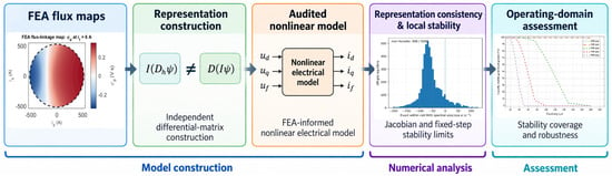
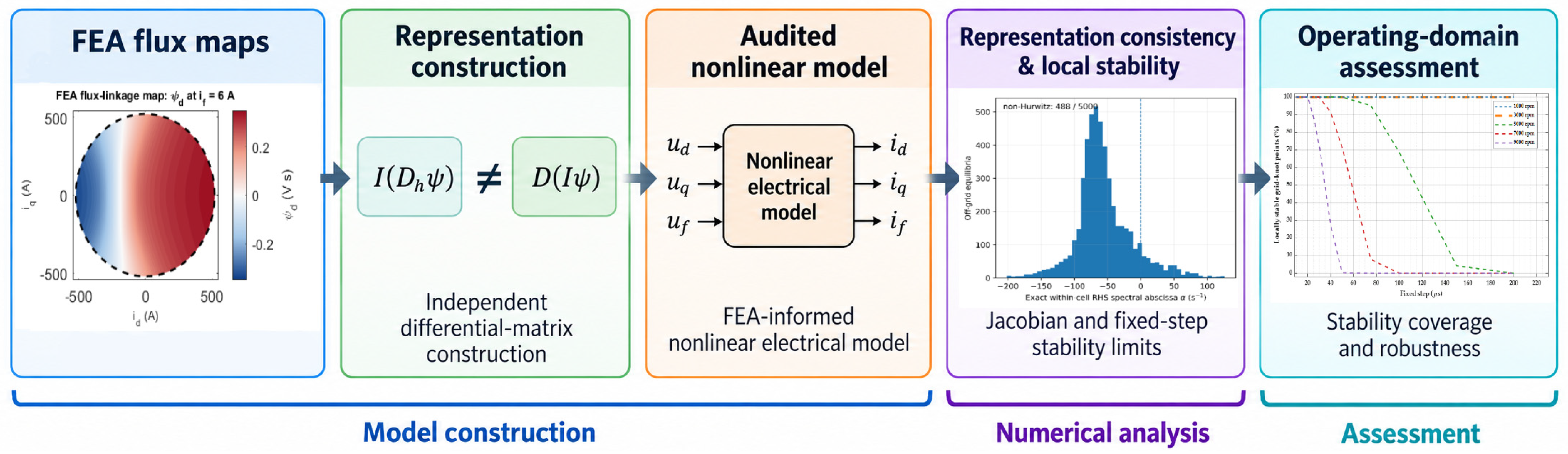
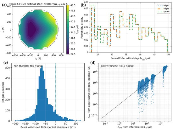
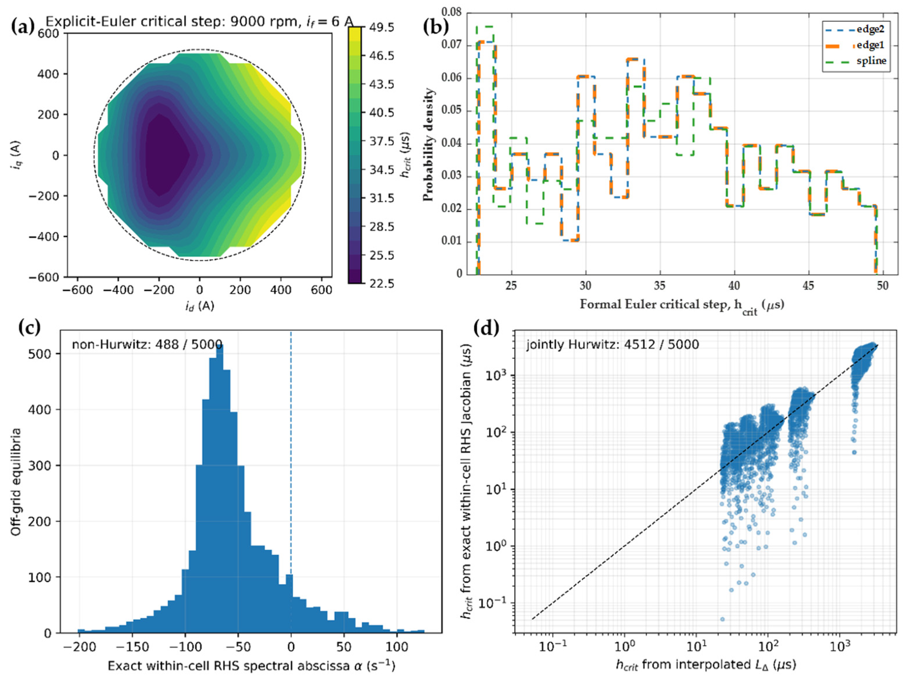
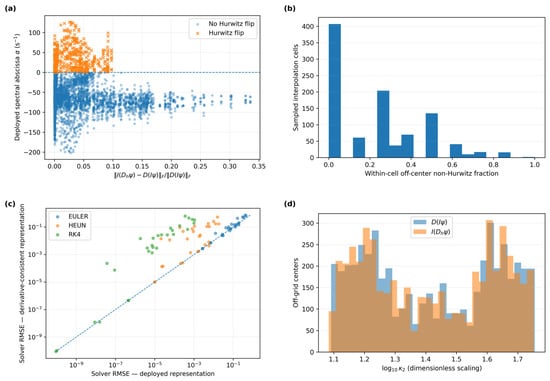
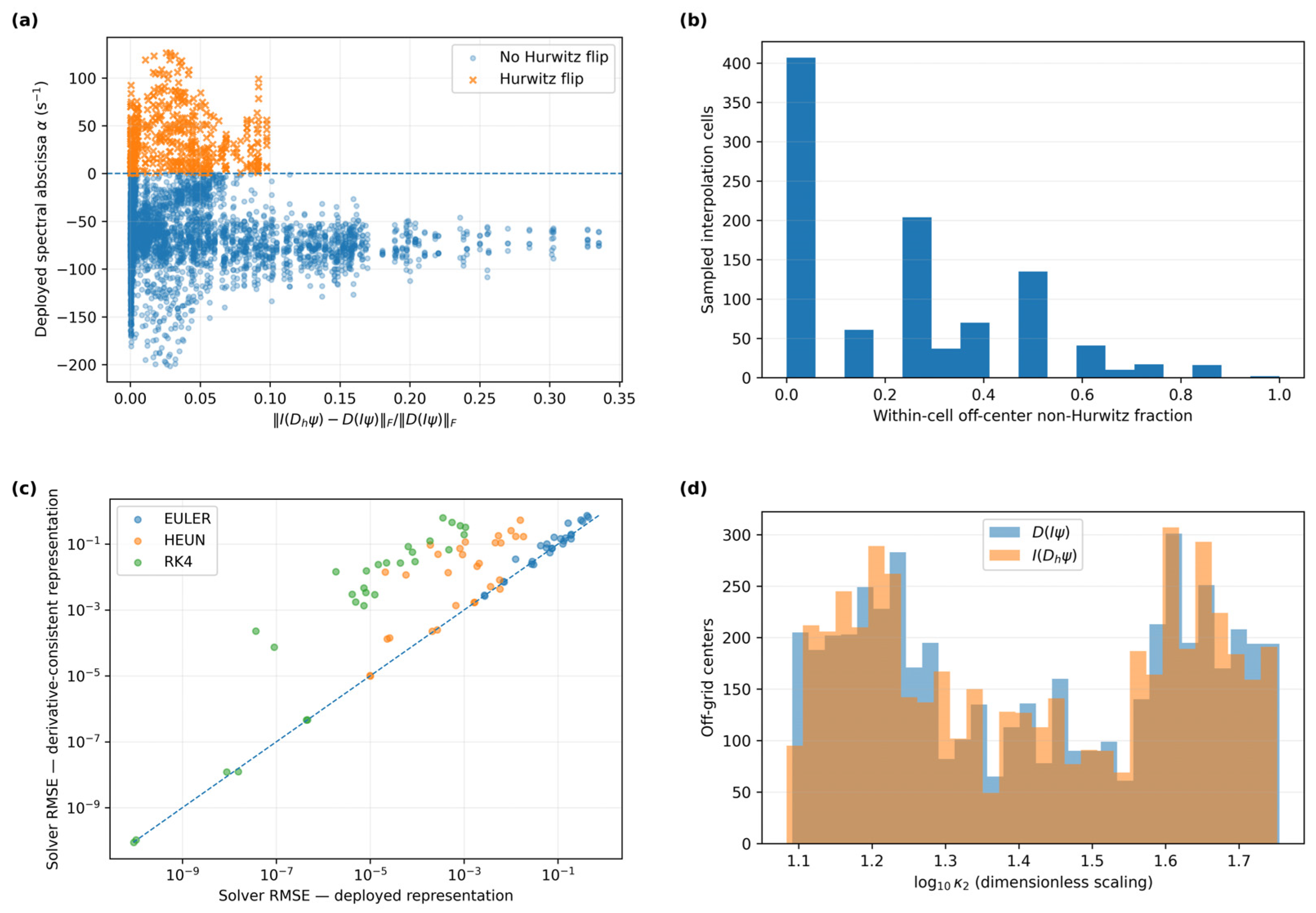
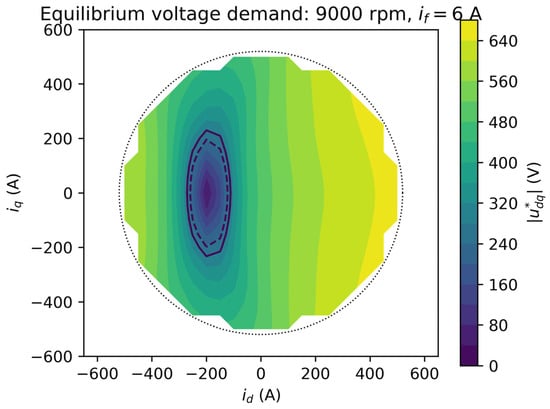
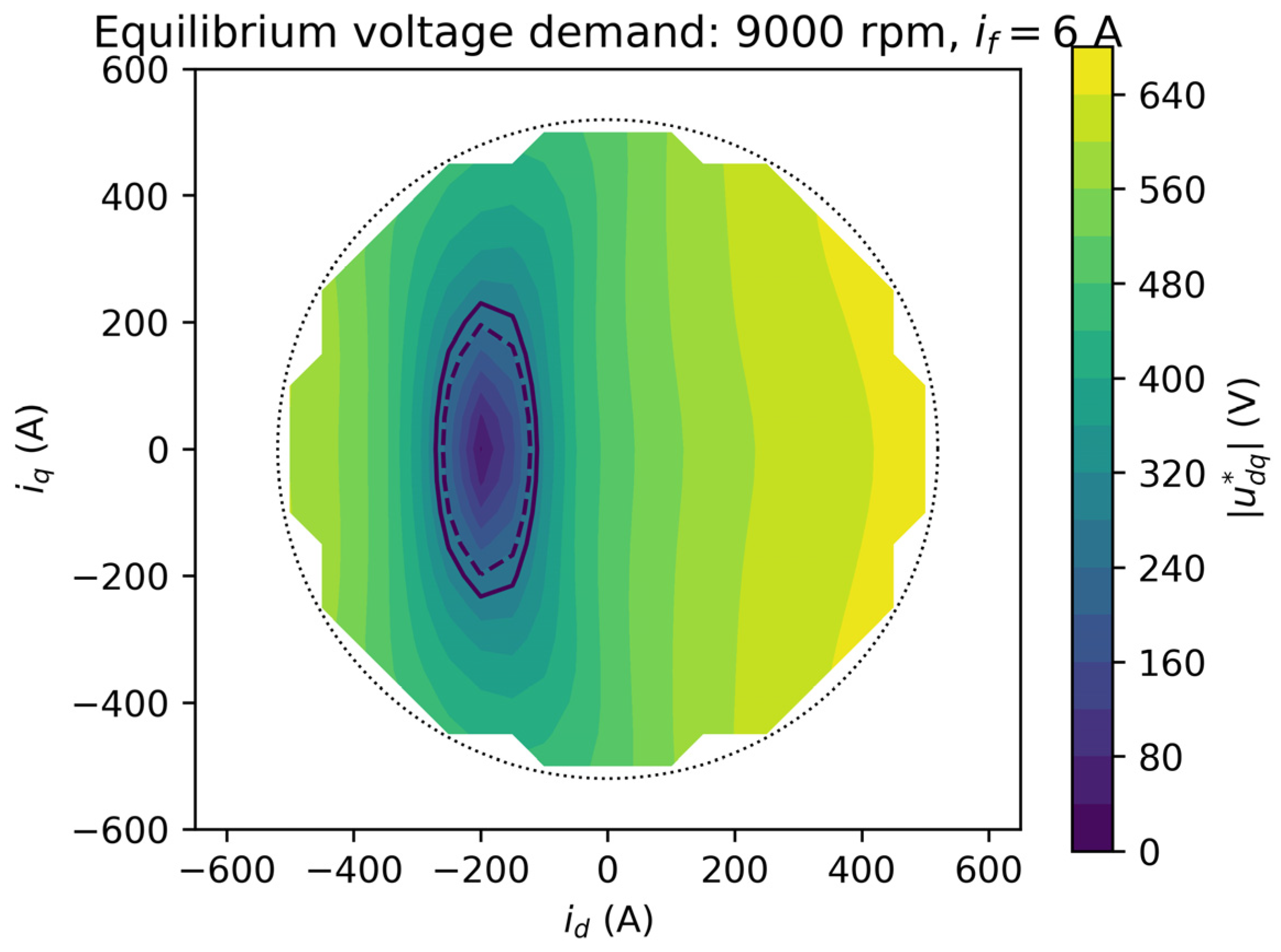
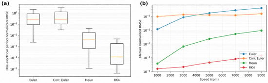
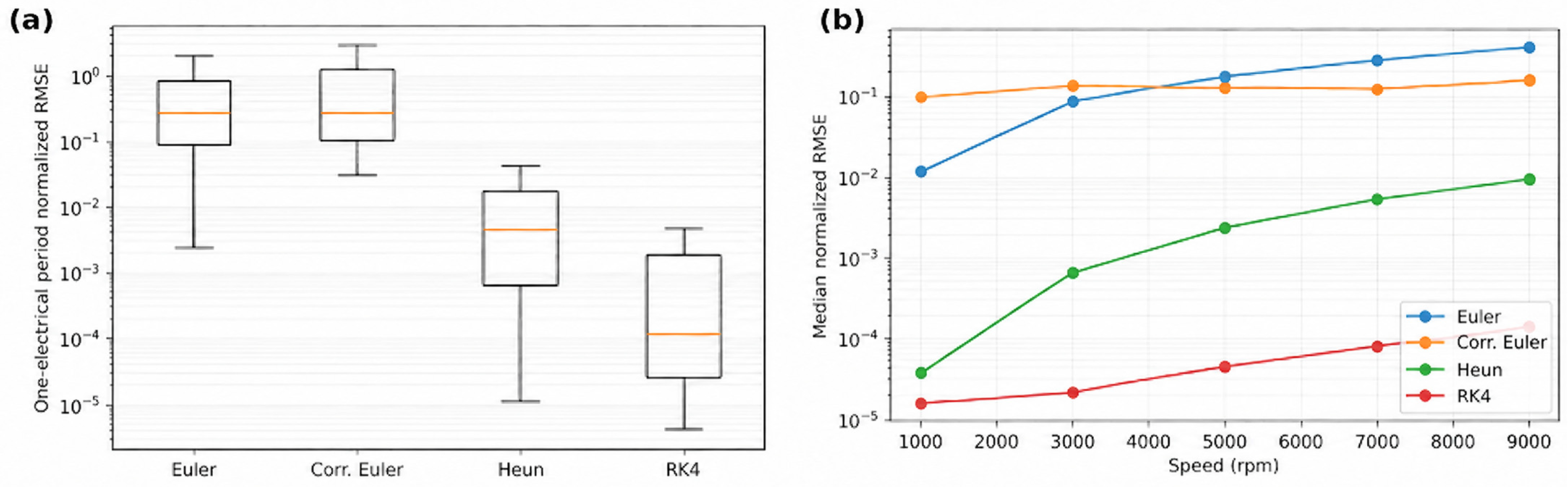
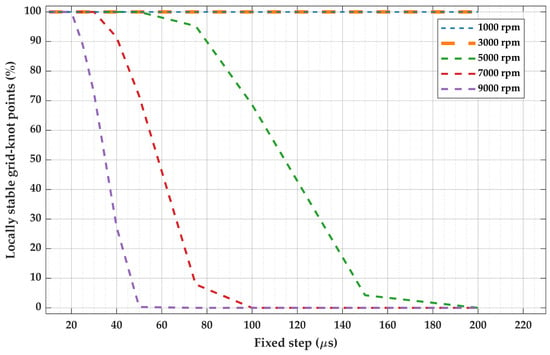
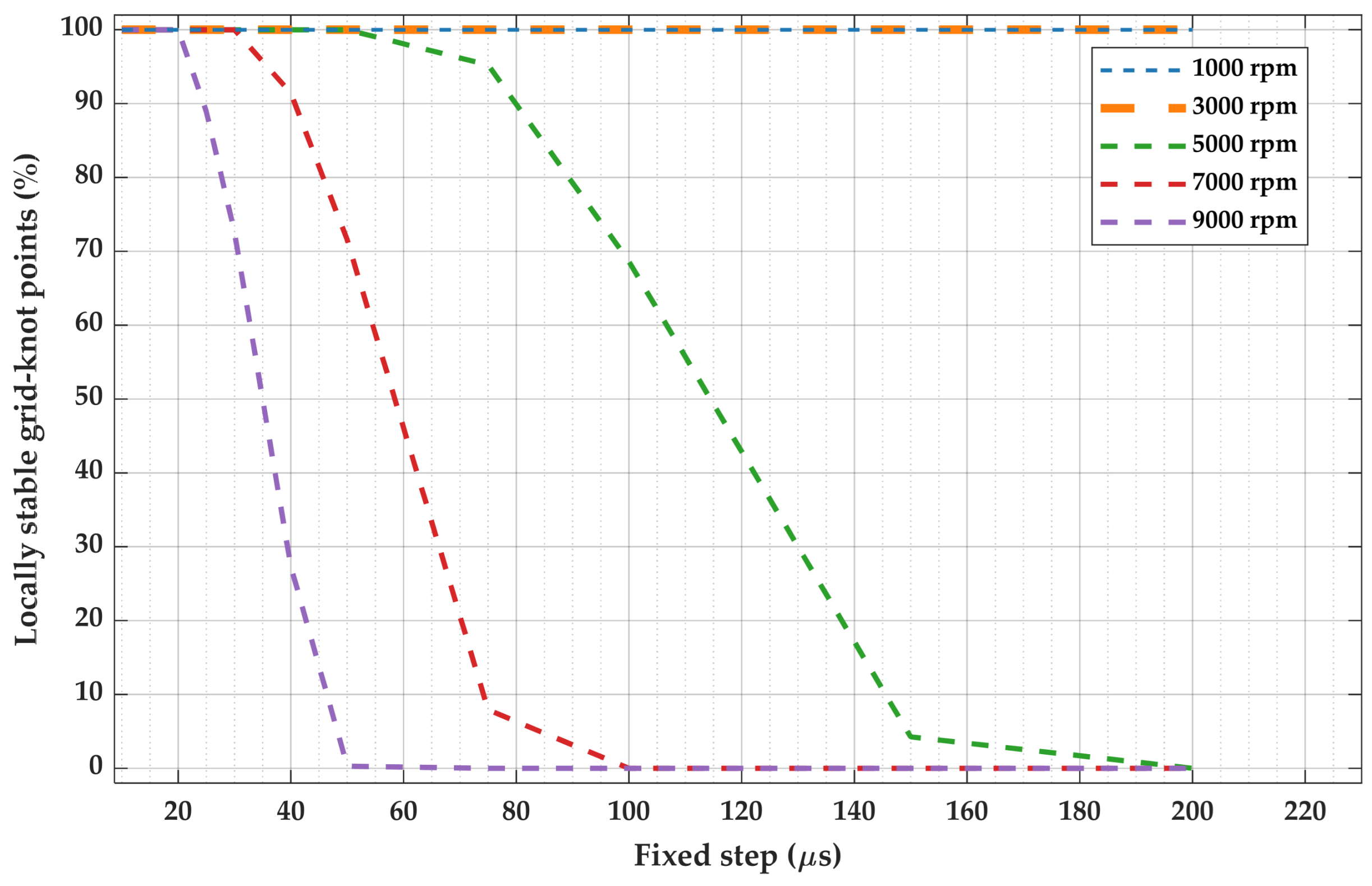

Disclaimer/Publisher’s Note: The statements, opinions and data contained in all publications are solely those of the individual author(s) and contributor(s) and not of MDPI and/or the editor(s). MDPI and/or the editor(s) disclaim responsibility for any injury to people or property resulting from any ideas, methods, instructions or products referred to in the content. |
© 2026 by the author. Licensee MDPI, Basel, Switzerland. This article is an open access article distributed under the terms and conditions of the Creative Commons Attribution (CC BY) license.