ViL-UNet: Multi-Scale Global–Local Feature Fusion for High-Resolution Remote-Sensing Segmentation

Abstract

Efficiently extracting and integrating multi-scale global and local information remains a main challenge in remote-sensing semantic-segmentation tasks. Current convolutional neural networks (CNNs) can only capture fine-grained details but cannot model long-range dependencies. In contrast, sequence models, such as Transformer-based and Mamba-based models, have the ability to capture broad context. However, they have limitations in preserving local details. Recent hybrid architectures combine both to balance these strengths, but it is still difficult to fuse multi-scale global and local features in a unified and efficient manner. In this work, we propose ViL-UNet, a dual-branch encoder–decoder network, which addresses this challenge by combining a Vision-LSTM (ViL) global encoder with a CNN-based local encoder. The global encoder captures long-range dependencies across multiple scales. Furthermore, the local encoder preserves fine spatial details. We also design a novel Multi-Scale Fusing Module to integrate these complementary representations by resizing the global and local features to a common spatial grid, concatenating them, and generating a unified feature representation that captures broad contextual cues and fine-grained local information. The decoder applies Efficient Global–Local Attention and Squeeze-and-Excitation. In addition, the skip connections bring the fused multi-scale features back to higher resolutions. To demonstrate ViL-UNet’s effectiveness, we compared it against state-of-the-art methods on the ISPRS Vaihingen and LoveDA Urban benchmarks. Across both datasets, ViL-UNet consistently delivers more accurate semantic segmentation by efficiently capturing multi-scale global and local context in large-scale remote-sensing scenes.

1. Introduction

Recently, some advances in high-resolution remote sensing have led to several new usages like object detection [1], autonomous driving [2], and environmental monitoring [3]. These usages are based on the thorough understanding of each pixel in extensive areas. The semantic segmentation of remote-sensing images, i.e., assigning a semantic label to each pixel, is important for investigating objects and land cover over wide regions. The success of such segmentation hinges on capturing rich context at multiple scales.

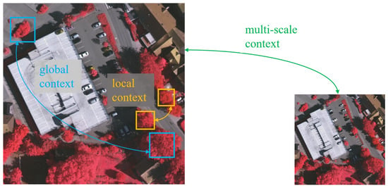
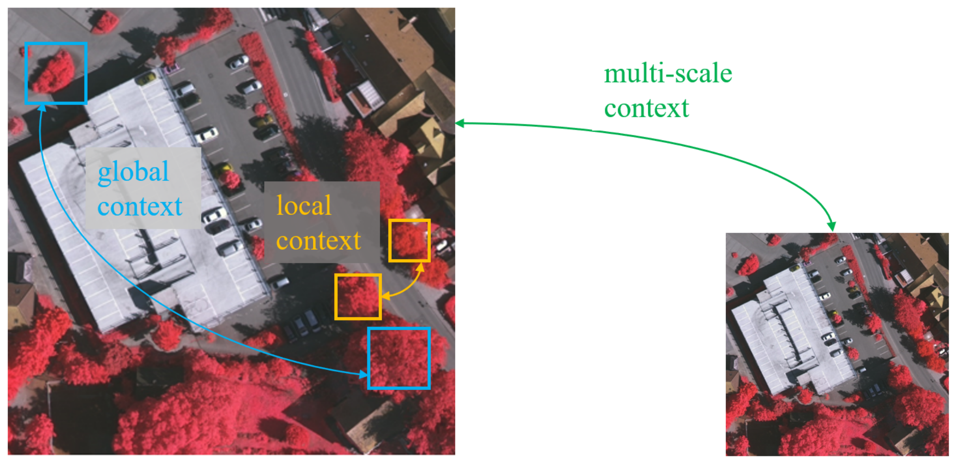
In large-scale remote-sensing images, objects vary dramatically in size and distribution, so the performance of segmentation is strongly tied to the ability to capture multi-scale global and local contexts in large-scale scenes [4,5]. The multi-scale global and local contexts are illustrated in Figure 1. Classic CNN-based methods address this via multi-scale feature extraction. For instance, the Pyramid Scene Parsing Network (PSPNet) [6] and the DeepLab family [5] use spatial pyramid pooling or atrous spatial pyramid pooling to obtain context at different scales. Although these methods enlarge the receptive field, they may lose some detailed information and cannot distinguish between different categories. The encoder–decoder structures like U-Net [7] and SegNet [8] employ hierarchical convolution and skip connections to restore the original features. Nevertheless, most CNNs generally have small receptive fields, which are not appropriate for dealing with long-range dependencies. Some attention mechanisms based on CNNs have been introduced to solve this problem; for example, Coordinate Attention [9] integrates the spatial coordinates into the channel attention, assisting the network in recognizing objects more accurately.

Figure 1. Illustration of Multi-Scale Global and Local Contexts in Remote-Sensing Images.

Recently, sequence-modeling techniques in NLP have been applied to vision to improve global context modeling. The Vision Transformer (ViT) [10] has global self-attention for long-range dependencies, and its windowed versions like the Swin Transformer [11] use a hierarchical and shifted-window approach to reduce the computational cost. They can obtain global semantics, but they have some difficulties in preserving the local details in segmentation tasks. Hybrid models attempt to combine the advantages of CNNs and Transformers. For instance, TransUNet [12] and UNetFormer [4] incorporate transformer modules into the U-Net structure to acquire local and global information at the same time. Nevertheless, the combination of multi-scale features from different parts is still a challenging problem and an important research area.

Currently, such sequence models are also being explored for visual tasks. The xLSTM [13] enhances traditional LSTMs with exponential gating and matrixized memory. They can improve the model’s parallelism and capacity. Alkin et al. [14] extend this idea to images in Vision-LSTM (ViL), arranging xLSTM blocks in alternating raster-scan directions (i.e., one block processes each row left-to-right, the next right-to-left). This bidirectional alternation allows ViL to aggregate context both horizontally and vertically with linear complexity. In practice, ViL has been shown to outperform ViT [10] and the Mamba state-space model [15] in capturing global context efficiently. These properties show that ViL is suitable to be the backbone for high-resolution remote-sensing segmentation, and understanding the entire scene is crucial.

In this paper, we propose ViL-UNet, a dual-branch encoder–decoder network for remote-sensing semantic-segmentation tasks. The global encoder branch uses Vision-LSTM modules to capture long-range context, and the local encoder branch extracts fine-grained spatial details via convolutional layers. Furthermore, we also introduce a novel Multi-Scale Fusing Module (MSFM) to efficiently integrate the multi-scale features from both branches at each resolution. Finally, our decoder is designed by integrating Efficient Global–Local Attention (EGLA) and a Squeeze-and-Excitation (SE) module [16]. Both can adaptively combine skip-connected features and restore high-fidelity segmentation maps. Our main contributions are:

• We propose ViL-UNet, a dual-branch encoder that integrates Vision-LSTM for multi-scale global context modeling with a CNN-based local branch for fine-grained spatial representation in remote-sensing segmentation.
• We design a Multi-Scale Fusing Module (MSFM) to combine global and local features at each scale. Channel Attention and Spatial Attention are used to reweight the fused features, allowing the model to better handle different spatial contexts and object sizes.
• We incorporate Efficient Global–Local Attention (EGLA) and Squeeze-and-Excitation (SE) in our decoder to adaptively merge skip-connected features and produce high-fidelity segmentation outputs.

2. Related Works

Remote-Sensing Semantic segmentation has developed rapidly with the advances of deep learning. Early methods always used convolutional networks to extract local texture and shape features. More recent studies have explored sequence models to capture global context. Hybrid architectures combine these two approaches. In the following, we review representative methods in three categories and discuss their strengths and limitations, which provides the motivation for our ViL-UNet design.

2.1. CNN-Based Segmentation Methods

Most of the early semantic-segmentation models for remote-sensing images were built on convolutional architectures. Fully Convolutional Networks (FCNs) [17] were the first to enable end-to-end dense prediction by replacing the final classification layers with $1\times 1$ convolutions. FCN variants (FCN-32s, FCN-16s, FCN-8s) fuse coarse, high-level features with finer, low-level feature maps with skip connections. This fusion improves spatial detail, but outputs still have blurred boundaries and always miss long-range context. To sharpen edges, SegNet introduced an encoder–decoder design that reuses max-pooling indices during upsampling [8]. Furthermore, DeepLabv1 built on FCN, using atrous convolutions to enlarge receptive fields. It also applies a fully connected CRF to refine segmentation maps. Subsequent DeepLab variants introduced more context aggregation: DeepLabv2’s Atrous Spatial Pyramid Pooling (ASPP) [18], DeepLabv3 added image-level pooling plus batch normalization [19], and DeepLabv3+ further incorporates a lightweight decoder to recover spatial details, notably improving boundary delineation for narrow objects [5].

The U-Net family has played an important role in remote sensing. ResUNet-a combines the traditional U-Net with residual connections for further training, atrous convolutions, and a Pyramid Scene Parsing module to obtain multi-scale context. It uses several supervisory signals such as edges and distance maps [20,21]. Furthermore, UNet++ incorporates nested dense skip connections to improve the features at various scales, thus enhancing the segmentation of small objects [22]. Moreover, Attention U-Net introduces spatial and channel attention mechanisms into U-Net, which can adjust the weights of the feature maps adaptively. This feature helps in identifying sparse classes such as cars and lampposts [23]. However, these modified U-Net models are good at depicting local details but depend on fixed convolution kernels and local receptive fields, which restrict their ability to handle the global context in large homogeneous areas.

Although some improvement has been achieved, the pure CNN-based methods are still locally sensitive. This has been shown in recent research, where a fixed-size convolution kernel leads to a small effective receptive field, which is insufficient for detecting long-range dependencies and comprehending the whole scene. Therefore, researchers have introduced modules like dilated convolutions, pyramid pooling, and self-attention to improve the contextual information, such as in ASPP of DeepLab [19] and SPP of PSPNet [6], or to enhance the details [5,24,25]. In summary, the CNN-based approaches are good at modeling local features and maintaining clear edges, but they generally cannot deal with global features properly.

2.2. Sequence-Modeling Methods (Transformers and Mamba)

Transformer-based models and related sequence approaches aim to capture global context. UNetFormer embeds a transformer-style global–local attention into a U-Net decoder, using a CNN encoder (e.g., ResNet18) for multi-scale features and a dual-branch decoder: a global-attention branch that partitions high-resolution maps into windowed multi-head self-attention (akin to Swin Transformer) to model long-range relationships, and a local branch of CNN layers to recover edges and textures [4]. TransUNet treats image patches as tokens fed to a Vision Transformer (ViT) encoder, capturing long-range coherence across large objects but at high computational cost [12], with TransUNet++ adding multi-scale skip connections and cross-attention to reinforce small-object details [26]. Other variants—PVT [27], UPerNet [28], SegFormer [29], Swin-Unet [30], and HRNet [31]—each explore multi-scale fusion strategies.

Mamba-based modules (state-space models) achieve linear-time global context modeling. Rs-Mamba replaces the ViT backbone with a “Mamba” module, extracting multi-scale feature maps, splitting them into patch sequences, and using an Omnidirectional Selective Scanning Module (OSSM) to scan patches along multiple orientations before applying state-space layers [32]. Inspired by Hyena’s implicit filters [33], S4’s structured state-space layers [34], and AxialAttention’s factorization [35], Rs-Mamba achieves competitive accuracy with reduced inference time and memory.

Recently, several studies have also explored Vision-LSTM (ViL) for visual representation and remote-sensing segmentation. Seg-LSTM [36] mainly uses Vision-LSTM for feature representation without an explicit parallel CNN branch for local feature extraction, whereas MMDNet [37] employs dual global–local branches but does not use the same U-Net-style hierarchical encoder–decoder with explicit multi-scale fusion. ViL-UNet combines hierarchical global and local encoders with MSFM and hierarchical decoding.

In general, sequence models excel at global context: Vision Transformers model segmentation as a sequence to sequence task, effectively extracting features with long range dependencies [10]. However, they often do so at high computational cost and can under-emphasize local details. The emergence of hybrid designs (see next) reflects a desire to obtain the best of both: CNN inductive biases for local structure, plus transformer/mamba style global context.

2.3. Dual-Branch Hybrid CNN–Sequence Architectures

Dual-branch hybrids explicitly combine CNN and sequence pathways. SSNet [38] is one example: it runs a CNN branch and a Transformer branch in parallel, exchanging information between them. SSNet’s Feature Fusion Module (FFM) includes several sub-modules with attention and pooling to merge various types of features, and its Feature Injection Module (FIM) uses strip convolutions and Squeeze-and-Excitation blocks to inject global information into the CNN during downsampling, improving the ability to recognize narrow structures. A CNN-like decoder with ASPP and skip connections is then applied to improve the combined representations. This architecture achieves good results in complex urban scenes by effectively integrating local and global information. Other methods such as SETR [39], K-Net [40], Mask2Former [41] and MaxViT [42] also present different fusion techniques to integrate detailed and broad context features.

State-space dual-branch models have been studied as well: for example, RS³Mamba [43] uses a ResNet-18 CNN branch for local details and a multi-directional Mamba branch based on VMamba [15] for global context with linear-time complexity. Its Collaborative Context Module integrates the two branches by element-wise addition, which ensures the efficiency of inference but fixes the fusion weights, thus not being able to adjust the emphasis between local and global features at different object scales. Similarly, other related structures such as TransFuse [44], GLU [45], CoAtNet [46], BiSeNet [47], and FastFCN [48] emphasize the necessity of maintaining both local and global information, yet none can completely solve the problem of adaptive and scale-sensitive feature fusion.

2.4. Summary and Motivation

In conclusion, CNN-based techniques are good at modeling local features and preserving edges but have difficulty in considering the whole scene. The Transformer and Mamba models are effective in handling long-range dependencies; however, they may ignore some detailed information and consume much computing power. Hybrid architectures can solve this problem, but usually use fixed or simple methods for combination. It is necessary to develop a unified and efficient way to combine multi-scale global and local features. Thus, we propose ViL-UNet with its Multi-Scale Fusing Module (MSFM), which combines the global context of Vision-LSTM with the local features of CNN and uses Channel Attention and Spatial Attention for adjustable weighting. In the following section, the architecture and main components of ViL-UNet will be introduced.

3. Methodology

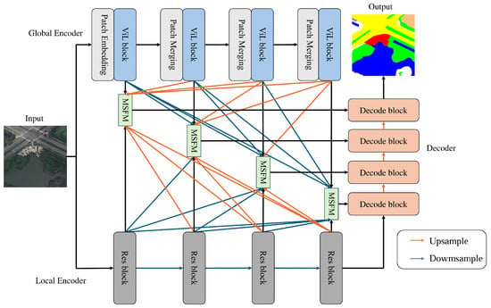
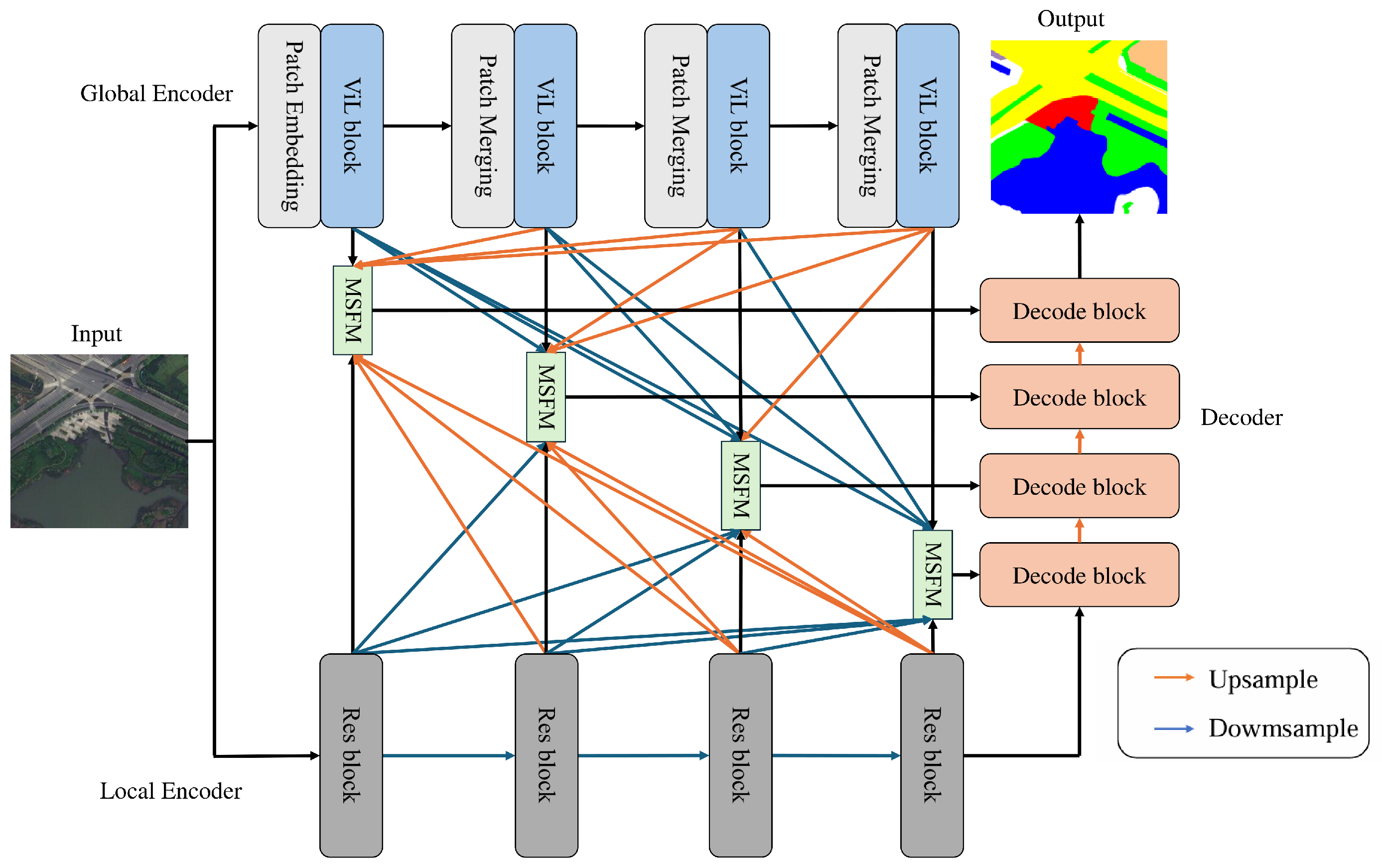
The overall architecture of ViL-UNet comprises four key parts: a global encoder, a local encoder, a Multi-Scale Fusing Module (MSFM), and a decoder, as shown in Figure 2. The dual-branch encoder obtains both global and local features at four different hierarchical levels from RS images. Specifically, the global encoder utilizes Vision-LSTM (ViL) [14] modules to recognize long-range dependencies and summarize coarse, scene-level context, whereas the local encoder is based on a pretrained ResNet18 backbone to extract fine details. After that, the multi-scale features, including both global and local contexts, are sent to MSFM, which effectively combines features at different scales and simultaneously integrates global and local spatial semantic contexts. Unlike ASPP [19], which depends on fixed dilation rates, MSFM performs parallel convolutions with variable kernels before adaptive channel and spatial attention, thus covering a wider range of receptive fields. Unlike FPN [49], which merges features by means of simple top-down pathways, MSFM synthesizes all scales into a unified representation and refines it through Channel Attention and Spatial Attention, integrating multi-scale convolutions with lightweight windowed self-attention to achieve a balance between efficiency and expressiveness. The decoder uses Efficient Global–Local Attention (EGLA) and a Squeeze-and-Excitation (SE) module [16], and then applies skip connections to obtain the fused multi-scale global–local features from MSFM for the final prediction map reconstruction.

Figure 2. Framework of ViL-UNet. Black arrows indicate standard feature transmission, orange arrows indicate upsampling, and blue arrows indicate downsampling.

3.1. Global Encoder

The Global Encoder in ViL-UNet includes four hierarchical stages, in which the spatial resolution is reduced while capturing wider contexts progressively. In the first stage, the input image $X\in {\mathbb{R}}^{H\times W\times C}$ is divided into non-overlapping patches of size $P\times P$. Each patch is then linearly mapped to a token embedding, forming a sequence of $\left(\frac{H}{P}\times \frac{W}{P}\right)$ tokens, each of dimension C. In each following stage, adjacent tokens are combined so that the spatial dimensions are decreased to half, and the channel depth is increased to twice, guaranteeing that the later stages process fewer but more semantically rich tokens.

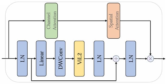
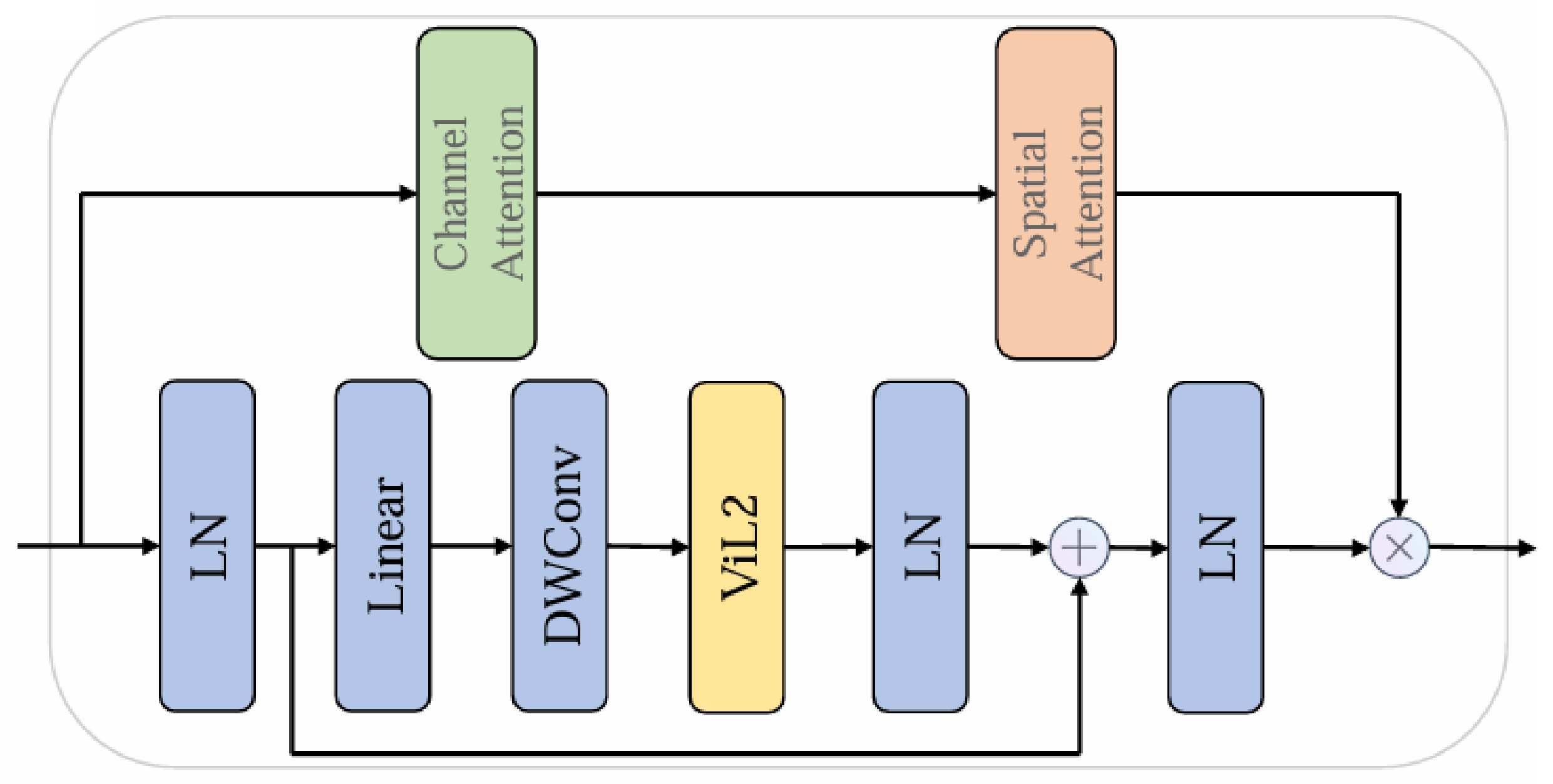
At each scale, we employ a Vision-LSTM block (Figure 3) that splits its input $\widehat{X}$ into two parallel branches. The first branch applies Channel Attention followed by Spatial Attention to adaptively emphasize informative channels and spatial regions, thereby sharpening features [50]. The second branch is the core Vision-LSTM2 (ViL2) component [13,14], which captures global context with linear complexity. Letting

$$\widehat{X}=[x_1,x_2,\dots ,x_N],N={\displaystyle \frac{H}{P}}\times {\displaystyle \frac{W}{P}},$$

(1)

the j-th mLSTM block reorders its input tokens according to

$${\widehat{X}}^{\left(j\right)}=\left[x_{{\sigma }_j\left(1\right)},x_{{\sigma }_j\left(2\right)},\dots ,x_{{\sigma }_j\left(N\right)}\right],$$

(2)

$${\sigma }_j\left(i\right)=\left\{\begin{array}{cc}i,\hfill & j\mathrm{odd}\left(\mathrm{left}\text{-}\mathrm{to}\text{-}\mathrm{right}\right),\hfill \\ N+1-i,\hfill & j\mathrm{even}\left(\mathrm{right}\text{-}\mathrm{to}\text{-}\mathrm{left}\right).\hfill \end{array}\right.$$

(3)

Each reordered sequence ${\widehat{X}}^{\left(j\right)}$ is then processed by an mLSTM cell, whose operations—input, forget, output gates, and state updates—operate sequentially in one direction. By alternating left-to-right and right-to-left raster scans across layers, ViL2 enables bidirectional contextual aggregation over the 2D feature grid. Although no explicit column-wise scan is used, the recurrent state propagates across rows along the raster sequence, allowing information to flow in both horizontal and vertical directions while retaining $O\left(N{d}^2\right)$ complexity rather than the $O\left(N^2\right)$ complexity of traditional self-attention, where d is the token embedding dimension.

Figure 3. The ViL block architecture in the global encoder, using Vision-LSTM as its core to capture global context.

The outputs from the two branches are fused via element-wise addition and a final linear projection to form the global feature map $F_G^i$ at stage i. This hybrid design combines Channel and Spatial attention’s capacity to highlight salient channels and spatial regions with Vision-LSTM’s efficient bidirectional context modeling, enabling ViL-UNet to capture comprehensive global semantics in high-resolution remote-sensing images.

3.2. Vision-LSTM2 (ViL2) Structure

The ViL2 module is composed of multiple block-pairs, each containing two mLSTM layers that traverse the token sequence in opposite directions to achieve bidirectional context aggregation with linear complexity. We first map the input image $X\in {\mathbb{R}}^{H\times W\times C}$ into a sequence of N tokens of dimension d via a patch embedding layer and add 2D positional embeddings, yielding

$${\mathbf{z}}_0\in {\mathbb{R}}^{B\times N\times d},N={\displaystyle \frac{H}{P}}\times {\displaystyle \frac{W}{P}},$$

(4)

where B is the batch size, P is the patch size, and d is the embedding dimension.

Each mLSTM layer updates its hidden and cell states using linear gating and an attention-like mechanism. Let ${\mathbf{x}}_t\in {\mathbb{R}}^d$ be the t-th token in the sequence. Then at step t, the mLSTM computes:

$$\begin{array}{cc}\hfill q_t& =W_q{\mathbf{x}}_t+{\mathbf{b}}_q,\hfill \end{array}$$

(5)

$$\begin{array}{cc}\hfill k_t& ={\displaystyle \frac{1}{\sqrt{d}}}{W}_k{\mathbf{x}}_t+{\mathbf{b}}_k,\hfill \end{array}$$

(6)

$$\begin{array}{cc}\hfill v_t& =W_v{\mathbf{x}}_t+{\mathbf{b}}_v,\hfill \end{array}$$

(7)

where $W_q,W_k,W_v\in {\mathbb{R}}^{d\times d}$ and ${\mathbf{b}}_q,{\mathbf{b}}_k,{\mathbf{b}}_v\in {\mathbb{R}}^d$ are learned projection weights and biases for queries, keys, and values, respectively. The input gate $i_t$, forget gate $f_t$, and output gate $o_t$ are computed as

$$\begin{array}{cc}\hfill {\tilde{i}}_t& ={\mathbf{w}}_i^{\top }{\mathbf{x}}_t+b_i,i_t=\exp \left({\tilde{i}}_t\right),\hfill \end{array}$$

(8)

$$\begin{array}{cc}\hfill {\tilde{f}}_t& ={\mathbf{w}}_f^{\top }{\mathbf{x}}_t+b_f,f_t=\exp \left({\tilde{f}}_t\right),\hfill \end{array}$$

(9)

$$\begin{array}{cc}\hfill {\tilde{o}}_t& =W_o{\mathbf{x}}_t+{\mathbf{b}}_o,o_t=\sigma \left({\tilde{o}}_t\right),\hfill \end{array}$$

(10)

where ${\mathbf{w}}_i,{\mathbf{w}}_f\in {\mathbb{R}}^d$, $b_i,b_f\in \mathbb{R}$, and $W_o\in {\mathbb{R}}^{d\times d}$, ${\mathbf{b}}_o\in {\mathbb{R}}^d$. Please note that $i_t$ uses an exponential to ensure positivity, while $f_t$ uses an exponential for stability.

The cell state ${\mathbf{C}}_t$ and an auxiliary “normalizer” state ${\mathbf{n}}_t$ are updated as

$$\begin{array}{cc}\hfill {\mathbf{C}}_t& =f_t{\mathbf{C}}_{t-1}+i_t{v}_t{k}_t^{\top },\hfill \end{array}$$

(11)

$$\begin{array}{cc}\hfill {\mathbf{n}}_t& =f_t{\mathbf{n}}_{t-1}+i_t{k}_t,\hfill \end{array}$$

(12)

where ${\mathbf{C}}_{t-1}\in {\mathbb{R}}^{d\times d}$ and ${\mathbf{n}}_{t-1}\in {\mathbb{R}}^d$. The product $v_t{k}_t^{\top }$ is a rank-1 outer product that updates the memory matrix, while ${\mathbf{n}}_t$ accumulates the key vectors for numerical normalization.

The hidden state ${\mathbf{h}}_t\in {\mathbb{R}}^d$ is obtained by first computing a gated candidate ${\tilde{\mathbf{h}}}_t$ and then applying the output gate:

$$\begin{array}{cc}\hfill {\tilde{\mathbf{h}}}_t& ={\displaystyle \frac{{\mathbf{C}}_t{q}_t}{\max \left\{{\mathbf{n}}_t^{\top }{q}_t,1\right\}}},\hfill \end{array}$$

(13)

$$\begin{array}{cc}\hfill {\mathbf{h}}_t& =o_t\odot {\tilde{\mathbf{h}}}_t,\hfill \end{array}$$

(14)

where ⊙ denotes element-wise multiplication. The denominator $\max \{{\mathbf{n}}_t^{\top }{q}_t,1\}$ prevents division by small values, providing numerical stability.

By alternating between left-to-right (odd) and right-to-left (even) scans, each block-pair updates its hidden representations according to

$${\mathbf{z}}_{\ell }={\mathrm{mLSTM}}_{\mathrm{even}}\left({\mathrm{mLSTM}}_{\mathrm{odd}}\left({\mathbf{z}}_{\ell -1}\right)\right),\ell =1,\dots ,L,$$

(15)

where ${\mathrm{mLSTM}}_{\mathrm{odd}}$ and ${\mathrm{mLSTM}}_{\mathrm{even}}$ use the same formulas above (Equations (5)–(14)) but scan token indices in opposite directions. This bidirectional alternation enables each token to aggregate information from its entire sequence with $\mathcal{O}\left(N{d}^2\right)$ complexity, significantly more efficient than standard self-attention’s $\mathcal{O}\left(N^{2}d\right)$.

To improve generalization, stochastic depth (drop-path) with a rate of 0.05 is applied to the output of each block-pair. Finally, a LayerNorm produces the normalized output:

$${\mathbf{z}}_L^{\mathrm{norm}}=\mathrm{LayerNorm}\left({\mathbf{z}}_L\right).$$

(16)

In conclusion, the mLSTM equations (Equations (5)–(14)) describe how the cell and hidden states of each token are updated through gated outer-product memory and normalized query–key interactions, which allow efficient and bidirectional context modeling appropriate for high-resolution remote sensing.

3.3. Multi-Scale Fusing Module (MSFM)

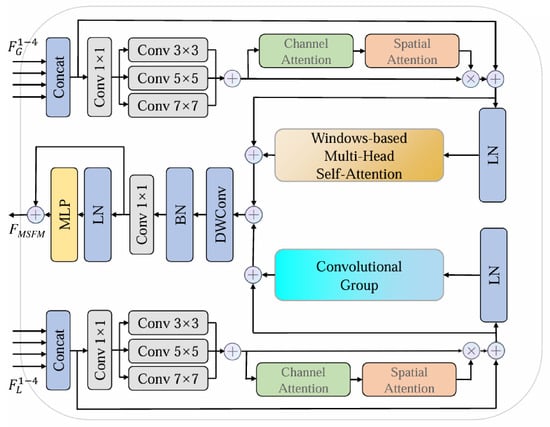
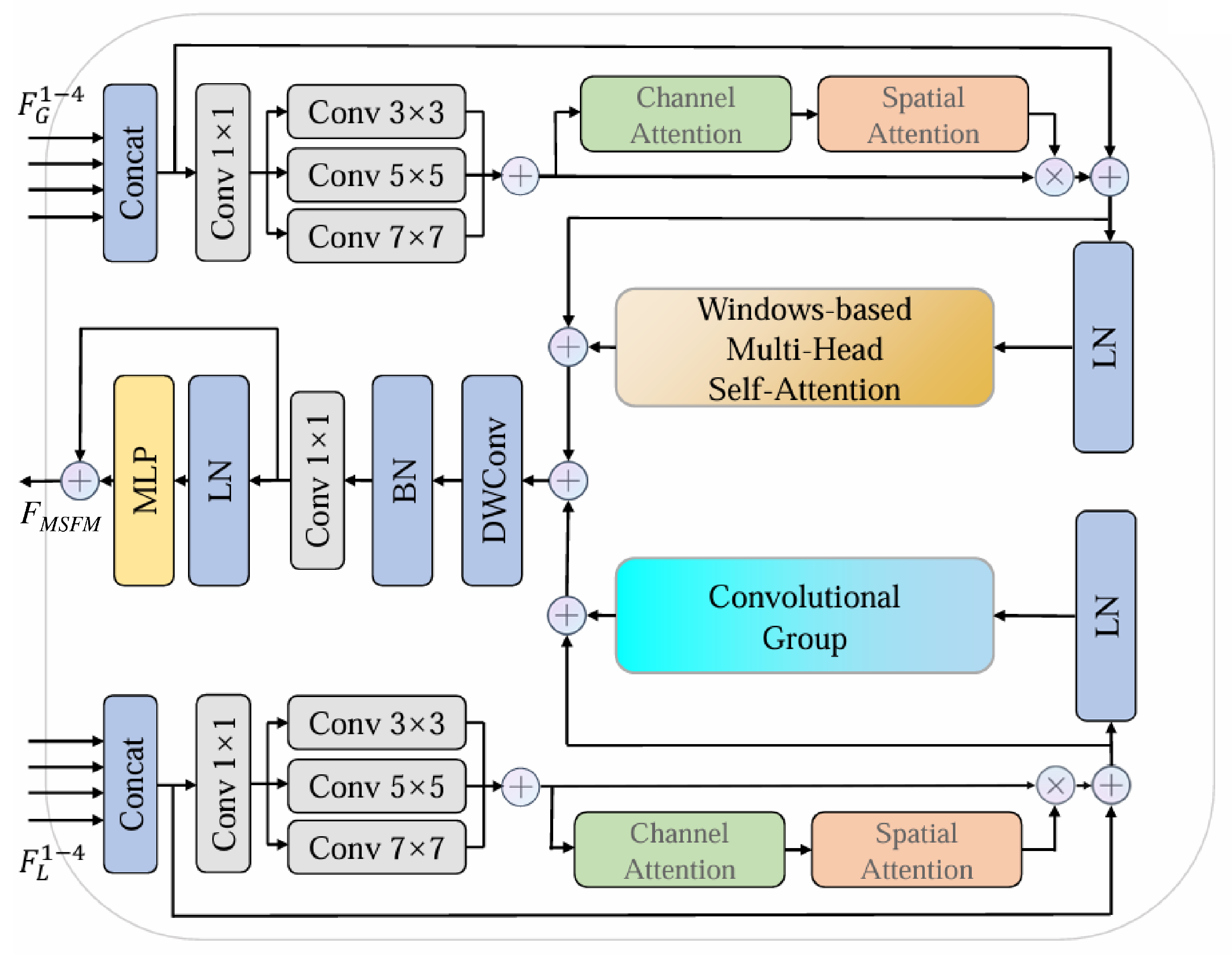
Figure 4 illustrates the Multi-Scale Fusing Module (MSFM), which is intended to combine hierarchically obtained features from both the global and local encoders into a unified and high-capacity representation. First, we resize each of the four output feature maps from the global encoder ${\left\{F_G^i\right\}}_{i=1}^4$ and the local encoder ${\left\{F_L^i\right\}}_{i=1}^4$ to the same spatial resolution, by using trainable upsampling for the low-resolution maps and strided convolution for the high-resolution maps. After all eight tensors have the same height $H^{\prime }$ and width $W^{\prime }$, we join the four maps of each branch along the channel direction:

$${\widehat{F}}_G=\left[F_G^1,F_G^2,F_G^3,F_G^4\right],{\widehat{F}}_L=\left[F_L^1,F_L^2,F_L^3,F_L^4\right].$$

(17)

This combination gathers data from various encoder layers and enlarges the channel dimension.

Figure 4. The MSFM architecture, which fuses multi-scale features from both encoder branches.

To obtain the same dimensionality, each tensor after concatenation is processed into C channels by a lightweight $1\times 1$ convolution. Then, ${\tilde{F}}_G$ and ${\tilde{F}}_L$ are, respectively, introduced into three parallel convolutional sequences with kernel sizes of $3\times 3$, $5\times 5$ and $7\times 7$. These parallel branches are used to extract different spatial features with different receptive fields—the small kernels focus on edges and fine textures, while the large kernels take into account the whole context. At last, the outputs of these parallel sequences are summed up to obtain a complete multi-scale response.

$$F_{\mathrm{ms}}={\mathrm{Conv}}_{3\times 3}\left(\tilde{F}\right)+{\mathrm{Conv}}_{5\times 5}\left(\tilde{F}\right)+{\mathrm{Conv}}_{7\times 7}\left(\tilde{F}\right),$$

(18)

where $\tilde{F}$ represents the projected features of either branch. Batch normalization and a nonlinear activation (GELU) are applied after each convolution to stabilize the training process and enhance the representation.

We use a two-stage attention scheme for each $F_{\mathrm{ms}}$. The Channel Attention modifies the feature channels according to their overall significance, whereas the Spatial Attention highlights the important spatial positions and reduces the less significant responses [50]. Such procedures improve the refined multi-scale feature representation.

Finally, the attended global and local feature maps are combined in a hybrid fusion block which considers both long-distance and local interactions. One branch uses window-based multi-head self-attention, dividing the feature map into non-overlapping windows of size $M\times M$ and calculating:

$$\mathrm{Attention}(Q,K,V)=\mathrm{softmax}\left({\displaystyle \frac{Q{K}^{\top }}{\sqrt{d_k}}}\right)V,$$

(19)

Efficiently, a global context model is established in each window. The parallel branch divides the channels into several groups using grouped convolution for separate processing, to enhance local coherence and preserve fine details. Then, the two obtained results are summed up and fed into layer normalization to obtain the final fused representation $F_{\mathrm{MSFM}}$.

By employing multi-scale convolutions, adaptive Channel and Spatial attention, and efficient windowed self-attention with grouped convolutions, MSFM generates a fine and context-related feature representation. The decoder then uses $F_{\mathrm{MSFM}}$ through skip connections to obtain accurate segmentation maps, thus obtaining a good balance between global semantic consistency and local edge sharpness.

3.4. Decode Block

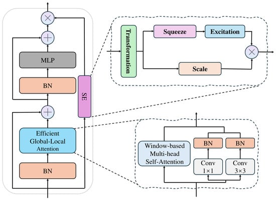
Figure 5 illustrates the Decode Block, which reconstructs the resolution and improves the feature representations through three parallel branches: the main Efficient Global–Local Attention (EGLA) [4] branch, the Squeeze–Excitation (SE) [16] branch, and a residual skip branch. After upsampling and concatenation with the corresponding encoder feature, the EGLA branch first conducts a $1\times 1$ convolution and a $3\times 3$ convolution, each followed by BatchNorm, to obtain local patterns with different receptive fields. Then, these two feature maps are added together and transformed into query, key, and value tensors for a window-based multi-head self-attention (W-MHSA) operation.

Figure 5. Structure of the decode block.

Within each non-overlapping $M\times M$ region, the W-MHSA, based on Equation (19), obtains the local contextual relations. No shifted-window technique is used. Instead, the cross-window contextual information is combined through horizontal and vertical pooling procedures, which assists the model in recognizing larger spatial relationships without increasing the computing cost. Then, the attention output is converted back to the original spatial scale and introduced into a BatchNorm to obtain the final result of the branch. This approach allows the EGLA to combine the detailed edge features extracted by the convolutional layers with the global context relations represented by the attention mechanism.

In the SE branch, the fused feature map $\mathbf{Y}\in {\mathbb{R}}^{H\times W\times C}$ is firstly “squeezed” by global average pooling into a channel descriptor

$$\begin{array}{cc}\hfill z_c& ={\displaystyle \frac{1}{HW}}{\displaystyle \sum _{i=1}^H}{\displaystyle \sum _{j=1}^W}{Y}_c(i,j),\hfill \end{array}$$

(20)

where $Y_c(i,j)$ indicates the activation at the spatial position $(i,j)$ of channel c, and $H,W$ represent the height and width. This step integrates the spatial information into a single scalar $z_c$, which reflects the importance of channel c in the whole feature map.

Next, the “excitation” step passes the vector $\mathbf{z}={[z_1,\dots ,z_C]}^{\top }$ through a two-layer bottleneck MLP:

$$\begin{array}{cc}\hfill \mathbf{s}& =\sigma \left({\mathbf{W}}_2\delta \left({\mathbf{W}}_1\mathbf{z}\right)\right),\hfill \end{array}$$

(21)

where ${\mathbf{W}}_1\in {\mathbb{R}}^{\frac{C}{r}\times C}$ and ${\mathbf{W}}_2\in {\mathbb{R}}^{C\times \frac{C}{r}}$ are the learned weight matrices (with reduction ratio r), $\delta (·)$ is the ReLU activation function to ensure nonlinearity, and $\sigma (·)$ is the sigmoid function which limits each element $s_c\in (0,1)$. This transformation allows the network to handle inter-channel dependencies and calculate adaptive gating coefficients $\mathbf{s}$ which indicate the relative importance of each channel.

Finally, the original feature map is “scaled” channel-wise by these gates:

$$\begin{array}{cc}\hfill Y_c^{\prime }(i,j)& =s_c{Y}_c(i,j),\hfill \end{array}$$

(22)

so that channels with larger $s_c$ (i.e., more relevant for the current segmentation task) are enhanced, while less significant channels are reduced. Consequently, these three procedures enable the SE branch to adjust the responses of the channels adaptively, improving the network’s emphasis on discriminative features and resulting in clearer and more precise segmentation.

The third branch transmits the concatenated input through an identity (residual) connection. The final output of the block is obtained by summing the element-wise outputs of the three streams. By integrating the efficient global–local fusion of EGLA with the channel-wise recalibration of SE and a direct skip connection, the Decode Block generates high-fidelity segmentation maps with both clear boundaries and consistent global structure.

3.5. Loss Function

To train ViL-UNet, we use a joint loss function that integrates the pixel-wise Cross-Entropy (CE) loss and the Dice loss. The CE loss offers stable supervision for each pixel and promotes convergence by punishing incorrect classifications; however, it is susceptible to class imbalance and may not perform well on small or sparse classes [17]. In contrast, the Dice loss optimizes the overlap between the prediction and the true values, which is beneficial for segmenting minority classes and small objects, but may encounter gradient instability when the predictions are close to zero [51].

$$\begin{array}{cc}\hfill L_{\mathrm{CE}}& =-{\displaystyle \frac{1}{N}}{\displaystyle \sum _{i=1}^N}{\displaystyle \sum _{c=1}^C}{y}_{i,c}\log p_{i,c},\hfill \end{array}$$

(23)

$$\begin{array}{cc}\hfill L_{\mathrm{Dice}}& =1-{\displaystyle \frac{1}{C}}{\displaystyle \sum _{c=1}^C}{\displaystyle \frac{2{\sum }_{i=1}^N{p}_{i,c}{y}_{i,c}+\epsilon }{{\sum }_{i=1}^N{p}_{i,c}+{\sum }_{i=1}^N{y}_{i,c}+\epsilon }},\hfill \end{array}$$

(24)

$$\begin{array}{cc}\hfill L& =\alpha L_{\mathrm{CE}}+(1-\alpha )L_{\mathrm{Dice}}.\hfill \end{array}$$

(25)

When N stands for the pixel number, C indicates the number of categories, $y_{i,c}\in \{0,1\}$ represents the true one-hot value and $p_{i,c}\in [0,1]$ is the predicted probability for the c-th category, the Dice coefficient is computed separately for each category and then averaged over all C categories, including the background category. A small constant $\epsilon$ is utilized to prevent division by zero, and $\alpha =0.5$ is selected to assign equal weight to the two loss functions.

4. Experiments

4.1. Dataset

To evaluate our model’s performance, we conduct experiments on two challenging benchmarks:

4.1.1. ISPRS Vaihingen

The ISPRS Vaihingen dataset, released by the International Society for Photogrammetry and Remote Sensing (ISPRS), is often employed as a benchmark for remote-sensing semantic segmentation and object detection. It includes the Vaihingen area in Germany and consists of 33 aerial images of different sizes, each with three channels (IR, R, G). Each pixel is labelled into five categories: Building, Tree, Low Vegetation, Car, and Impervious Surface. The ground sampling distance is about 9 cm. In our experiments, tiles 1, 3, 23, 26, 7, 11, 13, 28, 17, 32, 34 and 37 are used for training, while tiles 5, 21, 15 and 30 are used for testing. No separate validation set is used for hyperparameter tuning.

4.1.2. LoveDA Urban

The LoveDA dataset [52] includes various rural and urban scenes for domain adaptation research. We select the urban part, which consists of 1833 RGB images with a dimension of $1024\times 1024$ pixels and a ground sampling distance of 30 cm. The corresponding masks are single-channel grayscale images, showing seven types of land cover: Background, Building, Road, Water, Barren, Forest, and Agriculture. The dataset is divided into 1156 training images and 677 testing images. In our experiments, 578 images are used for training and 338 for testing from the LoveDA database. Half of the urban part is selected at alternating positions in the published ordering from the original training or testing sets due to the large quantity of images in the dataset.

These two sets of data include detailed, multi-scale land-cover information, suitable for evaluating the ViL-UNet’s ability to recognize and combine both global contexts and local fine features.

4.2. Evaluation Metrics

To evaluate the segmentation performance precisely, we apply both class-wise and mean metrics like the F1 score and Intersection over Union (IoU), which are usually used in remote-sensing and semantic-segmentation tests due to their capability to deal with class imbalance and to be interpreted at the pixel level.

For a certain class c, let $T{P}_c$, $F{P}_c$ and $F{N}_c$ denote the numbers of true positives, false positives and false negatives, respectively. The F1 score for class c is the harmonic mean of precision and recall:

$$\mathrm{F}{1}_c={\displaystyle \frac{2T{P}_c}{2T{P}_c+F{P}_c+F{N}_c}}.$$

(26)

The IoU for class c, which is also called the Jaccard index, evaluates the overlap between the predicted and true regions:

$${\mathrm{IoU}}_c={\displaystyle \frac{T{P}_c}{T{P}_c+F{P}_c+F{N}_c}}.$$

(27)

To summarize performance across all C classes, we report the mean F1 score (mF1) and mean IoU (mIoU) as:

$$\mathrm{mF}1={\displaystyle \frac{1}{C}}{\displaystyle \sum _{c=1}^C}\mathrm{F}{1}_c,\hspace{1em}\mathrm{mIoU}={\displaystyle \frac{1}{C}}{\displaystyle \sum _{c=1}^C}{\mathrm{IoU}}_c.$$

(28)

These metrics offer extra details: IoU focuses on the spatial overlap, whereas F1 considers both detection sensitivity and precision. The use of class-wise and mean metrics is beneficial for assessing different approaches, especially in the remote-sensing field with various class distributions.

4.3. Experimental Setup

Our experiments are carried out in PyTorch 2.2.1 and performed on a single NVIDIA GeForce RTX 3090 GPU with 24 GB of VRAM. The models are trained for 100 epochs with AdamW using an initial learning rate of $5\times {10}^{-5}$, a batch size of 10, a linear warm-up during the first 10% of the training steps, and cosine annealing. The ResNet-18 local encoder is initialized with ImageNet-pretrained weights, while the ViL-T global encoder is trained from scratch. UNetFormer uses a pretrained ResNet-18, TransUNet uses a pretrained ResNet-50/ViT-B, and SSNet and Rs-mamba are trained from scratch. Each experiment is independently repeated five times without fixing a random seed, and the reported results are averaged over the five runs. All competing methods are retrained using the same dataset splits, preprocessing, data augmentation, training protocol, and inference settings as our proposed method. Detailed training, inference, augmentation, TTA, and model hyperparameters are provided in Appendix A.

5. Results and Discussion

5.1. Effect of Global and Local Encoder

Comparing “Global only” and “Local only” in Table 1, the Local-only configuration attains mF1 of 89.74% and mIoU of 81.65% on ISPRS Vaihingen, outperforming the Global-only result of 88.97% mF1 and 80.26% mIoU. This advantage is due to the fact that the Local encoder emphasizes the fine-grained spatial details such as edges, textures, and small objects, which are important in high-resolution aerial images. Conversely, the Global encoder alone summarizes the overall scene context at the cost of not distinguishing clear boundaries, resulting in lower scores. On LoveDA Urban, the model that uses only the Local encoder obtains an mF1 value of 63.22% and an mIoU value of 47.03%, whereas the one using only the Global encoder has an mF1 value of 62.10% and an mIoU value of 45.75%. It can be seen that accurately separating the complex urban scenes depends mainly on the local texture and shape cues, which are maintained by the Local decoder through the use of high-resolution feature maps and skip connections.

Table 1. Ablation study on key components of ViL-UNet. “Global” and “Local” indicate single-branch configurations, while “Both” uses both encoder branches. Checkmarks (✔) denote enabled SE, MSFM, and EGLA modules. Metrics are reported on ISPRS Vaihingen and LoveDA Urban. The best results are in bold.

Configuration	SE	MSFM	EGLA	ISPRS Vaihingen (%)		LoveDA Urban (%)
				mF1	mIoU	mF1	mIoU
Global only			✔	88.97	80.26	62.10	45.75
Local only			✔	89.74	81.65	63.22	47.03
Both			✔	90.07	81.74	64.05	48.21
Both (w/o EGLA)				90.02	81.75	64.05	47.98
Both + SE	✔		✔	90.13	81.91	64.42	48.93
Both + SE + MSFM (w/o EGLA)	✔	✔		90.20	81.93	64.77	49.35
Both + SE + MSFM	✔	✔	✔	90.44	82.19	65.44	50.19

After combining both encoders (“Both”), their concatenated outputs are first transformed back to the target channel dimension using a $1\times 1$ convolution and then entered into the decoder. The dual-branch structure achieves an mF1 of 90.07% and an mIoU of 81.74% on Vaihingen, and an mF1 of 64.05% and an mIoU of 48.21% on LoveDA. The joint model makes use of the coarse and long-range context provided by the Global encoder to capture large homogeneous areas such as rooftops or roads, while the Local encoder provides detailed information for accurate boundary recovery. As shown in Table 1, combining the global and local branches improves mF1 over either single-branch configuration, while the subsequent MSFM further enhances the dual-branch representation. This indicates that the benefit of the global branch is more effectively realized through global–local fusion rather than by simply adding the global branch to the local pathway.

5.2. Effect of SE and MSFM Modules

The internal operations of MSFM are designed as a combined fusion module; deleting each individual operation would require rearranging the intermediate channel dimensions and the fusion process. Hence, MSFM is assessed at the module level.

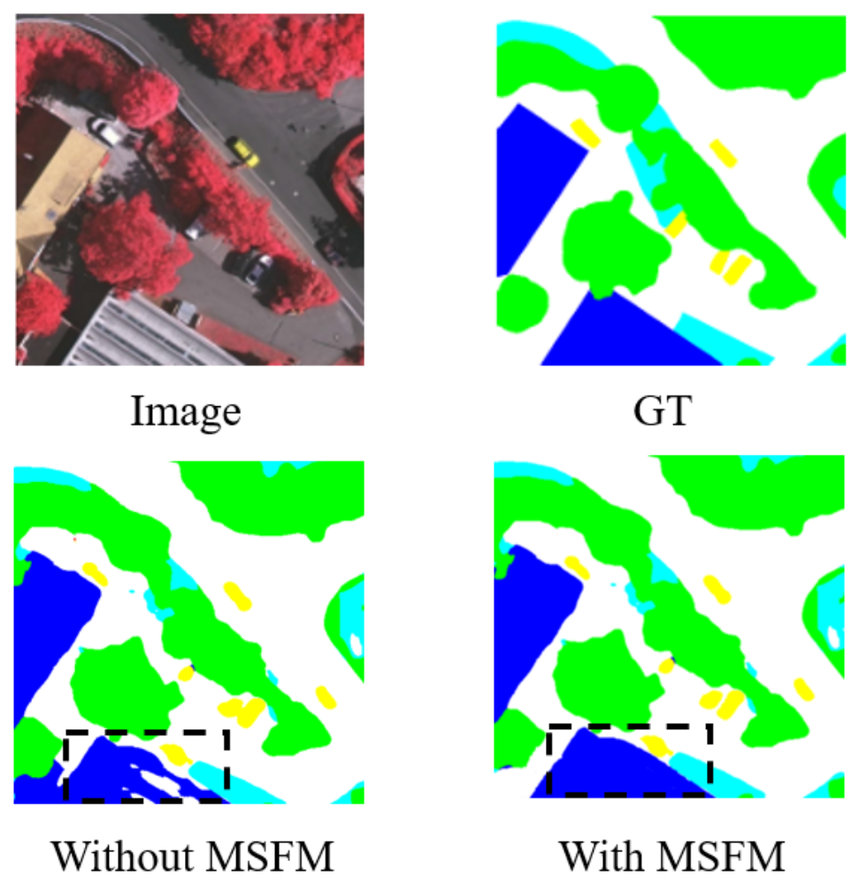
As described in Table 1, the addition of SE to the dual-branch baseline increases the mF1/mIoU from 90.07%/81.74% to 90.13%/81.91% on ISPRS Vaihingen and from 64.05%/48.21% to 64.42%/48.93% on LoveDA Urban. These improvements are due to the channel-wise calibration of SE, which strengthens the useful responses and reduces the irrelevant features. Furthermore, incorporating MSFM leads to an increase in mF1/mIoU to 90.20%/81.93% on Vaihingen and to 64.77%/49.35% on LoveDA Urban. When EGLA is also activated, the final results reach 90.44%/82.19% and 65.44%/50.19%, respectively. This enhancement is because of the hierarchical integration of multi-scale global and local features by MSFM, which offers more contextual and detailed representations. Figure 6 also indicates that the use of MSFM improves the boundary restoration and decreases the number of isolated misclassifications.

Figure 6. Qualitative comparison of segmentation results on the ISPRS Vaihingen dataset. From (top-left) to (bottom-right): original infrared image, ground truth (GT), prediction without the Multi-Scale Fusing Module (MSFM), and prediction with MSFM. The dashed boxes highlight regions where MSFM improves boundary accuracy and reduces misclassification.

5.3. Effect of EGLA Module

Table 1 further evaluates the effect of the Efficient Global–Local Attention (EGLA) module. When applied to the dual-branch baseline, EGLA produces only marginal changes: on ISPRS Vaihingen, mF1 changes from 90.02% to 90.07% and mIoU from 81.75% to 81.74%, while on LoveDA Urban, mF1 remains at 64.05% and mIoU increases from 47.98% to 48.21%. When SE and MSFM are further enabled, EGLA provides more noticeable gains, increasing mF1/mIoU from 90.20%/81.93% to 90.44%/82.19% on ISPRS Vaihingen and from 64.77%/49.35% to 65.44%/50.19% on LoveDA Urban. These findings indicate that EGLA works better on the enhanced and fused features generated by SE and MSFM, thereby improving the feature representation during the decoding process.

5.4. Effect of Different Global Encoder Backbones

Table 2 compares three lightweight global encoders—ViT-T, ViM-T and ViL-T—when used with the same local encoder and decoder on the ISPRS Vaihingen dataset. Although they have a similar number of parameters (approximately 51–57 M), ViL-T obtains the highest segmentation accuracy with an mF1 of 90.44% and mIoU of 82.19%. On the contrary, ViT-T achieves an mF1 of 90.13% and mIoU of 82.05%, while ViM-T has an mF1 of 90.21% and mIoU of 81.97%. It is noteworthy that ViL-T needs the least FLOPs (30.71 G), which is slightly less than ViT-T’s 30.89 G and ViM-T’s 32.24 G. This shows that ViL-T not only provides the highest precision but also performs the most efficiently in terms of computation, thus being the most suitable backbone for capturing the global context in high-resolution remote-sensing segmentation.

Table 2. Comparison of different global encoder backbones on the ISPRS Vaihingen dataset. All models share the same local encoder and decoder. The best results are in bold.

Global Encoder	Params (M)	FLOPs (G)	mF1 (%)	mIoU (%)
ViT-T [10]	51.64	30.89	90.13	82.05
ViM-T [53]	57.12	32.24	90.21	81.97
ViL-T [14]	51.73	30.71	90.44	82.19

5.5. Comparison with Other Methods

To show the effectiveness of ViL-UNet, we use UNetFormer [4], TransUNet [12], SSNet [38], and Rs-mamba [32] as main baselines, in which the first three are based on transformer architectures and the fourth is similar to a Mamba structure.

5.5.1. Results on the ISPRS Vaihingen Dataset

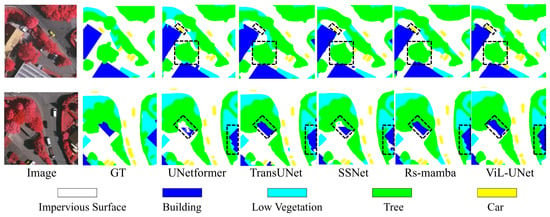
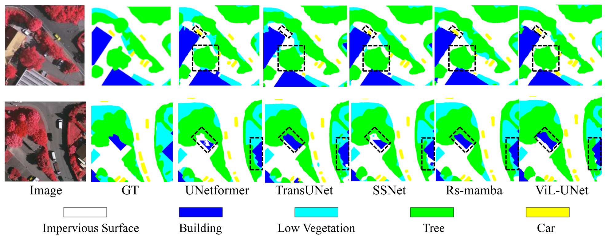
Table 3 presents per-class and overall F1 scores on the ISPRS Vaihingen benchmark. ViL-UNet achieves the highest mF1 of 90.44%, outperforming UNetFormer’s 89.70% by 0.74 percentage points, TransUNet’s 87.50%, SSNet’s 89.84%, and Rs-mamba’s 90.35%. It attains F1 scores of 93.41% on Impervious Surface, 97.54% on Building, and 91.93% on Tree, outperforming the corresponding baseline results. Table 4 reports the corresponding IoU values, with ViL-UNet achieving the highest mIoU of 82.19%, 0.44 points above UNetFormer’s 81.75%, and 86.65%, 94.05%, and 84.12% on Impervious Surface, Building, and Tree, respectively. Its relatively small standard deviation also indicates more stable performance across independent runs. Figure 7 shows representative examples, where ViL-UNet produces smoother and more coherent segmentation maps across object classes.

Table 3. F1 scores (%) on the ISPRS Vaihingen dataset. The best results are in bold.

Method	Backbone	Impervious Surface	Building	Low Vegetation	Tree	Car	mF1
UNetFormer [4]	ResNet-18	92.20	96.27	80.33	90.82	88.90	89.70 ± 0.05
TransUNet [12]	ResNet-50&ViT-B	90.71	94.25	79.03	90.49	83.01	87.50 ± 0.12
SSNet [38]	ViT-B	91.87	96.97	80.51	91.11	88.75	89.84 ± 0.08
Rs-mamba [32]	Mamba	91.74	97.46	80.73	91.77	90.03	90.35 ± 0.20
ViL-UNet	ResNet-18&ViL-T	93.41	97.54	80.68	91.93	88.59	90.44 ± 0.07

Table 4. mIoU scores (%) on the ISPRS Vaihingen dataset. The best results are in bold.

Method	Backbone	Impervious Surface	Building	Low Vegetation	Tree	Car	mIoU
UNetFormer [4]	ResNet-18	85.77	92.83	67.06	83.22	79.85	81.75 ± 0.08
TransUNet [12]	ResNet-50&ViT-B	82.91	89.03	65.38	82.63	70.97	78.18 ± 0.12
SSNet [38]	ViT-B	86.02	93.87	67.33	83.73	79.11	82.01 ± 0.12
Rs-mamba [32]	Mamba	84.12	94.03	67.61	84.02	80.66	82.09 ± 0.14
ViL-UNet	ResNet-18&ViL-T	86.65	94.05	67.41	84.12	78.71	82.19 ± 0.03

Figure 7. Qualitativecomparison of semantic-segmentation results on the ISPRS Vaihingen dataset. From (left) to (right): input image, ground truth (GT), and predictions from UNetFormer, TransUNet, SSNet, Rs-mamba, and ViL-UNet. Dashed boxes highlight regions of interest for visual comparison.

5.5.2. Results on the LoveDA Urban Dataset

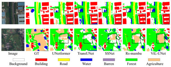
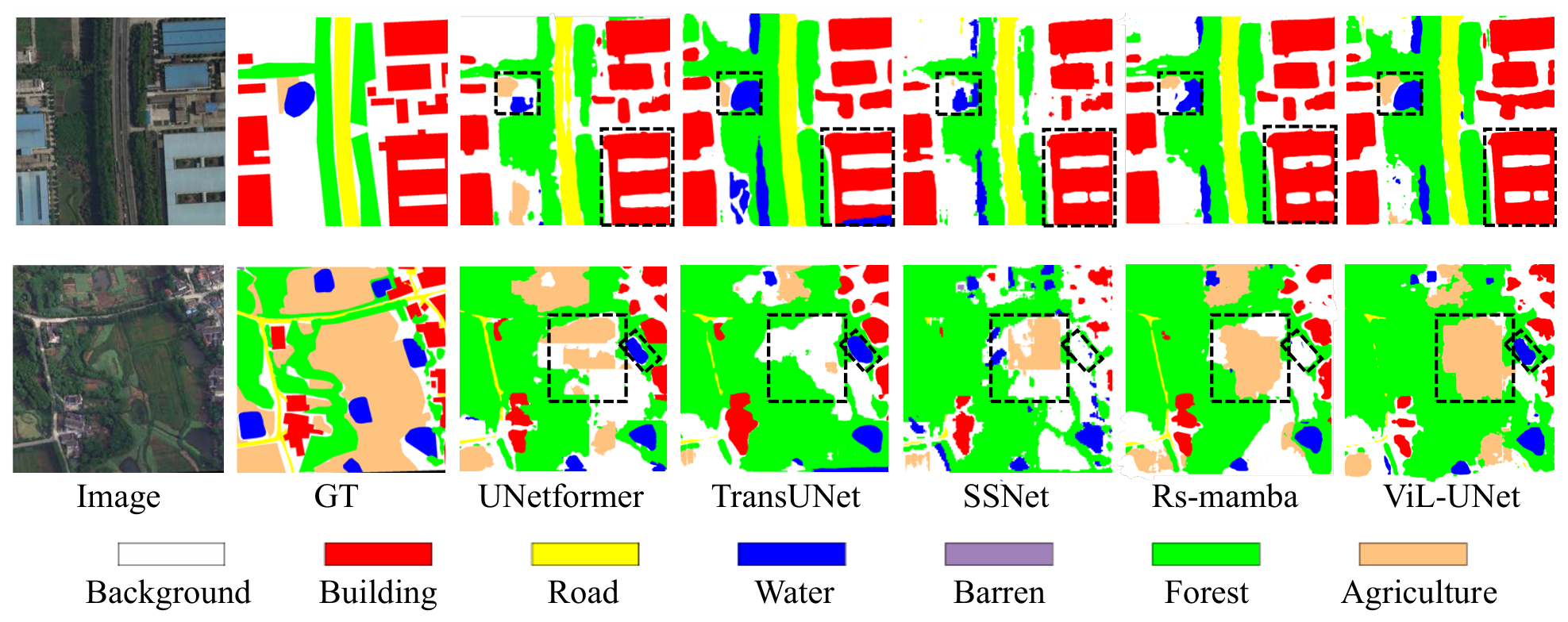
From Table 5 and Table 6, on the LoveDA Urban benchmark, the ViL-UNet obtains an mF1 of $65.44\%$ and an mIoU of $50.19\%$, which is better than that of UNetFormer by 1.30 and 1.28 percentage points, respectively. The improvements are more significant on difficult categories, with an F1 increase of 8.31 and 17.82 percentage points for Forest and Agriculture, respectively. ViL-UNet has less variation than Rs-mamba, suggesting a more stable performance in different trials. As depicted in Figure 8, the ViL-UNet segments small buildings, narrow roads, and dense vegetation more harmoniously, which indicates the effectiveness of the dual-branch structure and MSFM fusion.

Table 5. F1 scores (%) on the LoveDA Urban dataset. Each entry reports per-class F1 and overall mF1, with the best results in bold.

Method	Backbone	Background	Building	Road	Water	Barren	Forest	Agriculture	mF1
UNetFormer [4]	ResNet-18	60.52	76.09	75.16	85.20	63.46	56.47	32.06	64.14 ± 0.54
TransUNet [12]	ResNet-50&ViT-B	56.84	78.58	76.98	85.97	47.57	59.58	42.67	64.03 ± 2.28
SSNet [38]	ViT-B	61.18	79.44	75.27	80.82	49.83	56.13	47.32	64.28 ± 1.30
Rs-mamba [32]	Mamba	62.13	78.34	77.92	82.13	45.33	60.77	47.56	64.88 ± 3.42
ViL-UNet	ResNet-18&ViL-T	62.52	77.25	78.97	82.45	42.21	64.78	49.88	65.44 ± 1.77

Table 6. mIoU scores (%) on the LoveDA Urban dataset. Each entry reports per-class mIoU and overall mIoU, with the best results in bold.

Method	Backbone	Background	Building	Road	Water	Barren	Forest	Agriculture	mIoU
UNetFormer [4]	ResNet-18	42.60	59.92	58.56	71.96	46.24	39.51	23.58	48.91 ± 0.88
TransUNet [12]	ResNet-50&ViT-B	40.56	66.41	63.84	74.64	32.60	40.44	26.74	49.32 ± 1.90
SSNet [38]	ViT-B	44.54	69.33	60.12	66.01	36.50	39.08	32.13	49.67 ± 1.76
Rs-mamba [32]	Mamba	44.51	65.28	62.80	66.47	32.08	46.24	32.17	49.94 ± 3.54
ViL-UNet	ResNet-18&ViL-T	44.96	62.95	64.60	67.21	29.63	48.63	33.34	50.19 ± 1.82

Figure 8. Qualitative comparison of semantic-segmentation results on the LoveDA Urban dataset. From (left) to (right): input image, ground truth (GT), and predictions from UNetFormer, TransUNet, SSNet, Rs-mamba, and ViL-UNet. Dashed boxes highlight regions of interest for visual comparison.

5.5.3. Results for FLOPs, Params, MF1, and MIoU on ISPRS Vaihingen Dataset

As shown in Table 7, ViL-UNet has 51.73 M parameters and 44.32 G FLOPs, placing it within a moderate range of model complexity. Compared with Rs-mamba, ViL-UNet achieves higher mF1 (90.44% vs. 90.35%) and mIoU (82.19% vs. 82.09%), while requiring substantially fewer FLOPs (44.32 G vs. 87.77 G), achieving a higher inference speed (33.89 FPS vs. 26.54 FPS), and using less GPU memory (424.32 MB vs. 483.07 MB). Compared with the lighter UNetFormer and SSNet, ViL-UNet incurs higher computational cost but achieves better segmentation accuracy. These results indicate that ViL-UNet provides a favorable balance between segmentation accuracy and computational efficiency.

Table 7. Comparison of model complexity and segmentation performance on the ISPRS Vaihingen dataset. Metrics reported: number of parameters (in millions), FLOPs (in giga-FLOPs), inference speed (FPS), peak GPU memory (in MB), mean F1 (mF1) and mean IoU (mIoU) as percentages. The best results for each metric are in bold.

Method	Params (M)	FLOPs (G)	FPS	GPU Memory (MB)	mF1 (%)	mIoU (%)
UNetFormer [4]	48.37	22.93	40.48	290.14	89.70	81.75
TransUNet [12]	66.24	38.11	37.76	356.82	87.50	78.18
SSNet [38]	53.56	24.38	48.50	352.56	89.84	82.01
Rs-mamba [32]	52.37	87.77	26.54	483.07	90.35	82.09
ViL-UNet (ours)	51.73	44.32	33.89	424.32	90.44	82.19

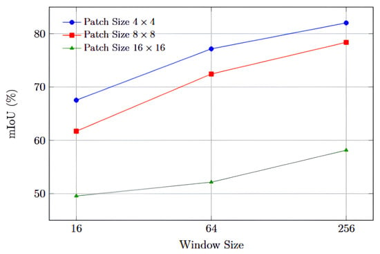
5.6. Sensitivity Analysis of Patch Size and Sliding-Window Size on mIoU

Figure 9 shows the sensitivity analysis of the overall ViL-UNet architecture with regard to the patch size and sliding-window size, evaluated by mIoU (%). According to our empirical results, larger sliding-window sizes can give a wider spatial context, whereas smaller patch sizes can maintain more detailed spatial information; we chose the commonly used 256 × 256 sliding-window size and, considering the hardware limitations, set the smallest feasible patch size to be 4 × 4 for the main experiments. The horizontal axis denotes the sliding-window sizes of 16, 64, and 256 pixels. When the patch size is 4 × 4, the mIoU increases from about 67.53% when the window size is 16 to 77.16% when the window size is 64 and reaches 82.03% when the window size is 256. When the patch size is $8\times 8$, mIoU starts at 61.71% for a window size of 16, increases to 72.44% at a window size of 64, and reaches 78.38% at a window size of 256. With the largest patch size of $16\times 16$, performance is lower across all window settings, beginning at 49.56% for a window size of 16, climbing to 52.16% at a window size of 64, and ending near 58.15% at a window size of 256. In all cases, larger sliding-window sizes yield higher mIoU, and the finest patch grid ($4\times 4$) benefits most from increasing the sliding-window size, suggesting that smaller patches combined with larger sliding windows capture long-range dependencies and fine-grained details more effectively and boost segmentation performance. These sensitivity experiments were not used for test-set-based hyperparameter selection, and the final configuration was fixed consistently across all main experiments.

Figure 9. Sensitivity analysis of mIoU (%) with respect to sliding-window size for three different patch sizes ($4\times 4$, $8\times 8$, and $16\times 16$) on the ISPRS Vaihingen dataset.

6. Conclusions

In this paper, we present ViL-UNet, a dual-branch encoder–decoder system for high-resolution remote-sensing semantic segmentation. The model integrates a Vision-LSTM-based global encoder to capture long-range dependencies at various scales with a CNN-based local encoder to maintain the detailed spatial information. The Multi-Scale Fusing Module (MSFM) merges these global and local characteristics into a unified representation. Then the decoder enhances the fused features using Efficient Global–Local Attention and Squeeze-and-Excitation methods, which results in precise segmentation maps. The experimental outcomes indicate that ViL-UNet achieves state-of-the-art accuracy while maintaining moderate model complexity. It is capable of acquiring both broad context and local accuracy, thus obtaining outstanding results on large uniform regions as well as fine structures. However, the use of Vision-LSTM and multi-branch fusion increases the memory consumption. Due to the current limited hardware resources, we have not evaluated ViL-UNet on larger data sets or carried out further studies in real-time segmentation situations. In our subsequent work, we intend to design lightweight strategies to achieve efficient real-time inference in high-precision remote-sensing applications.

References

- Li, K.; Wan, G.; Cheng, G.; Meng, L.; Han, J. Object detection in optical remote sensing images: A survey and a new benchmark. ISPRS J. Photogramm. Remote Sens. 2020, 159, 296–307. [Google Scholar] [CrossRef] [Scilit]
- Liu, Y.; Fan, B.; Wang, L.; Bai, J.; Xiang, S.; Pan, C. Semantic labeling in very high resolution images via a self-cascaded convolutional neural network. ISPRS J. Photogramm. Remote Sens. 2018, 145, 78–95. [Google Scholar] [CrossRef] [Scilit]
- Anand, T.; Sinha, S.; Mandal, M.; Chamola, V.; Yu, F.R. AgriSegNet: Deep aerial semantic segmentation framework for IoT-assisted precision agriculture. IEEE Sens. J. 2021, 21, 17581–17590. [Google Scholar] [CrossRef] [Scilit]
- Wang, L.; Li, R.; Zhang, C.; Fang, S.; Duan, C.; Meng, X.; Atkinson, P.M. UNetFormer: A UNet-like transformer for efficient semantic segmentation of remote sensing urban scene imagery. ISPRS J. Photogramm. Remote Sens. 2022, 190, 196–214. [Google Scholar] [CrossRef] [Scilit]
- Chen, L.C.; Zhu, Y.; Papandreou, G.; Schroff, F.; Adam, H. Encoder-decoder with atrous separable convolution for semantic image segmentation. In Proceedings of the European Conference on Computer Vision (ECCV); Springer: Cham, Switzerland, 2018; pp. 801–818. [Google Scholar]
- Zhao, H.; Shi, J.; Qi, X.; Wang, X.; Jia, J. Pyramid scene parsing network. In Proceedings of the IEEE Conference on Computer Vision and Pattern Recognition; IEEE: Piscataway, NJ, USA, 2017; pp. 2881–2890. [Google Scholar]
- Ronneberger, O.; Fischer, P.; Brox, T. U-net: Convolutional networks for biomedical image segmentation. In Proceedings of the Medical Image Computing and Computer-Assisted Intervention–MICCAI 2015: 18th International Conference, Munich, Germany, 5–9 October 2015; Proceedings, Part III 18; Springer: Cham, Switzerland, 2015; pp. 234–241. [Google Scholar]
- Badrinarayanan, V.; Kendall, A.; Cipolla, R. Segnet: A deep convolutional encoder-decoder architecture for image segmentation. IEEE Trans. Pattern Anal. Mach. Intell. 2017, 39, 2481–2495. [Google Scholar] [CrossRef] [Scilit]
- Hou, Q.; Zhou, D.; Feng, J. Coordinate attention for efficient mobile network design. In Proceedings of the IEEE/CVF Conference on Computer Vision and Pattern Recognition; IEEE: Piscataway, NJ, USA, 2021; pp. 13713–13722. [Google Scholar]
- Dosovitskiy, A.; Beyer, L.; Kolesnikov, A.; Weissenborn, D.; Zhai, X.; Unterthiner, T.; Dehghani, M.; Minderer, M.; Heigold, G.; Gelly, S.; et al. An image is worth 16x16 words: Transformers for image recognition at scale. arXiv 2020, arXiv:2010.11929. [Google Scholar]
- Liu, Z.; Lin, Y.; Cao, Y.; Hu, H.; Wei, Y.; Zhang, Z.; Lin, S.; Guo, B. Swin transformer: Hierarchical vision transformer using shifted windows. In Proceedings of the IEEE/CVF International Conference on Computer Vision; IEEE: Piscataway, NJ, USA, 2021; pp. 10012–10022. [Google Scholar]
- Chen, J.; Lu, Y.; Yu, Q.; Luo, X.; Adeli, E.; Wang, Y.; Lu, L.; Yuille, A.L.; Zhou, Y. Transunet: Transformers make strong encoders for medical image segmentation. arXiv 2021, arXiv:2102.04306. [Google Scholar]
- Beck, M.; Pöppel, K.; Spanring, M.; Auer, A.; Prudnikova, O.; Kopp, M.; Klambauer, G.; Brandstetter, J.; Hochreiter, S. xlstm: Extended long short-term memory. arXiv 2024, arXiv:2405.04517. [Google Scholar]
- Alkin, B.; Beck, M.; Pöppel, K.; Hochreiter, S.; Brandstetter, J. Vision-lstm: Xlstm as generic vision backbone. arXiv 2024, arXiv:2406.04303. [Google Scholar]
- Liu, Y.; Tian, Y.; Zhao, Y.; Yu, H.; Xie, L.; Wang, Y.; Ye, Q.; Jiao, J.; Liu, Y. Vmamba: Visual state space model. Adv. Neural Inf. Process. Syst. 2024, 37, 103031–103063. [Google Scholar] [CrossRef] [Scilit]
- Hu, J.; Shen, L.; Sun, G. Squeeze-and-excitation networks. In Proceedings of the IEEE Conference on Computer Vision and Pattern Recognition; IEEE: Piscataway, NJ, USA, 2018; pp. 7132–7141. [Google Scholar]
- Long, J.; Shelhamer, E.; Darrell, T. Fully convolutional networks for semantic segmentation. In Proceedings of the IEEE Conference on Computer Vision and Pattern Recognition; IEEE: Piscataway, NJ, USA, 2015; pp. 3431–3440. [Google Scholar]
- Chen, L.C.; Papandreou, G.; Kokkinos, I.; Murphy, K.; Yuille, A.L. Deeplab: Semantic image segmentation with deep convolutional nets, atrous convolution, and fully connected crfs. IEEE Trans. Pattern Anal. Mach. Intell. 2017, 40, 834–848. [Google Scholar] [CrossRef] [Scilit]
- Chen, L.C.; Papandreou, G.; Schroff, F.; Adam, H. Rethinking atrous convolution for semantic image segmentation. arXiv 2017, arXiv:1706.05587. [Google Scholar]
- Diakogiannis, F.I.; Waldner, F.; Caccetta, P.; Wu, C. ResUNet-a: A deep learning framework for semantic segmentation of remotely sensed data. ISPRS J. Photogramm. Remote Sens. 2020, 162, 94–114. [Google Scholar] [CrossRef] [Scilit]
- He, K.; Zhang, X.; Ren, S.; Sun, J. Deep residual learning for image recognition. In Proceedings of the IEEE Conference on Computer Vision and Pattern Recognition; IEEE: Piscataway, NJ, USA, 2016; pp. 770–778. [Google Scholar]
- Zhou, Z.; Rahman Siddiquee, M.M.; Tajbakhsh, N.; Liang, J. Unet++: A nested u-net architecture for medical image segmentation. In Proceedings of the Deep Learning in Medical Image Analysis and Multimodal Learning for Clinical Decision Support: 4th International Workshop, DLMIA 2018, and 8th International Workshop, ML-CDS 2018, Held in Conjunction with MICCAI 2018, Granada, Spain, 20 September 2018; Proceedings 4; Springer: Cham, Switzerland, 2018; pp. 3–11. [Google Scholar]
- Oktay, O.; Schlemper, J.; Folgoc, L.L.; Lee, M.; Heinrich, M.; Misawa, K.; Mori, K.; McDonagh, S.; Hammerla, N.Y.; Kainz, B.; et al. Attention u-net: Learning where to look for the pancreas. arXiv 2018, arXiv:1804.03999. [Google Scholar]
- Zhang, H.; Dana, K.; Shi, J.; Zhang, Z.; Wang, X.; Tyagi, A.; Agrawal, A. Context encoding for semantic segmentation. In Proceedings of the IEEE Conference on Computer Vision and Pattern Recognition; IEEE: Piscataway, NJ, USA, 2018; pp. 7151–7160. [Google Scholar]
- Fu, J.; Liu, J.; Tian, H.; Li, Y.; Bao, Y.; Fang, Z.; Lu, H. Dual attention network for scene segmentation. In Proceedings of the IEEE/CVF Conference on Computer Vision and Pattern Recognition; IEEE: Piscataway, NJ, USA, 2019; pp. 3146–3154. [Google Scholar]
- Du, Y.; Zhong, R.; Li, Q.; Zhang, F. TransUNet++ SAR: Change detection with deep learning about architectural ensemble in SAR images. Remote Sens. 2022, 15, 6. [Google Scholar] [CrossRef] [Scilit]
- Wang, W.; Xie, E.; Li, X.; Fan, D.P.; Song, K.; Liang, D.; Lu, T.; Luo, P.; Shao, L. Pyramid vision transformer: A versatile backbone for dense prediction without convolutions. In Proceedings of the IEEE/CVF International Conference on Computer Vision; IEEE: Piscataway, NJ, USA, 2021; pp. 568–578. [Google Scholar]
- Xiao, T.; Liu, Y.; Zhou, B.; Jiang, Y.; Sun, J. Unified perceptual parsing for scene understanding. In Proceedings of the European Conference on Computer Vision (ECCV); Springer: Cham, Switzerland, 2018; pp. 418–434. [Google Scholar]
- Xie, E.; Wang, W.; Yu, Z.; Anandkumar, A.; Alvarez, J.M.; Luo, P. SegFormer: Simple and efficient design for semantic segmentation with transformers. Adv. Neural Inf. Process. Syst. 2021, 34, 12077–12090. [Google Scholar]
- Cao, H.; Wang, Y.; Chen, J.; Jiang, D.; Zhang, X.; Tian, Q.; Wang, M. Swin-unet: Unet-like pure transformer for medical image segmentation. In Proceedings of the European Conference on Computer Vision; Springer: Cham, Switzerland, 2022; pp. 205–218. [Google Scholar]
- Sun, K.; Zhao, Y.; Jiang, B.; Cheng, T.; Xiao, B.; Liu, D.; Mu, Y.; Wang, X.; Liu, W.; Wang, J. High-resolution representations for labeling pixels and regions. arXiv 2019, arXiv:1904.04514. [Google Scholar]
- Zhao, S.; Chen, H.; Zhang, X.; Xiao, P.; Bai, L.; Ouyang, W. Rs-mamba for large remote sensing image dense prediction. IEEE Trans. Geosci. Remote Sens. 2024, 62, 5633314. [Google Scholar] [CrossRef] [Scilit]
- Nguyen, E.; Poli, M.; Faizi, M.; Thomas, A.; Wornow, M.; Birch-Sykes, C.; Massaroli, S.; Patel, A.; Rabideau, C.; Bengio, Y.; et al. Hyenadna: Long-range genomic sequence modeling at single nucleotide resolution. Adv. Neural Inf. Process. Syst. 2023, 36, 43177–43201. [Google Scholar] [CrossRef] [Scilit]
- Gu, A.; Goel, K.; Ré, C. Efficiently modeling long sequences with structured state spaces. arXiv 2021, arXiv:2111.00396. [Google Scholar]
- Wang, H.; Zhu, Y.; Green, B.; Adam, H.; Yuille, A.; Chen, L.C. Axial-deeplab: Stand-alone axial-attention for panoptic segmentation. In Proceedings of the European Conference on Computer Vision; Springer: Cham, Switzerland, 2020; pp. 108–126. [Google Scholar]
- Zhu, Q.; Cai, Y.; Fan, L. Seg-LSTM: Performance of xLSTM for semantic segmentation of remotely sensed images. arXiv 2024, arXiv:2406.14086. [Google Scholar]
- Ye, H.; Chang, J.; Wang, K.; Jia, Z.; Sun, W.; Li, Z. A lightweight multilevel multiscale dual-path fusion network for remote sensing semantic segmentation. Pattern Recognit. 2025, 172, 112483. [Google Scholar] [CrossRef] [Scilit]
- Yao, M.; Zhang, Y.; Liu, G.; Pang, D. SSNet: A novel transformer and CNN hybrid network for remote sensing semantic segmentation. IEEE J. Sel. Top. Appl. Earth Obs. Remote Sens. 2024, 17, 3023–3037. [Google Scholar] [CrossRef] [Scilit]
- Zheng, S.; Lu, J.; Zhao, H.; Zhu, X.; Luo, Z.; Wang, Y.; Fu, Y.; Feng, J.; Xiang, T.; Torr, P.H.; et al. Rethinking semantic segmentation from a sequence-to-sequence perspective with transformers. In Proceedings of the IEEE/CVF Conference on Computer Vision and Pattern Recognition; IEEE: Piscataway, NJ, USA, 2021; pp. 6881–6890. [Google Scholar]
- Zhang, W.; Pang, J.; Chen, K.; Loy, C.C. K-net: Towards unified image segmentation. Adv. Neural Inf. Process. Syst. 2021, 34, 10326–10338. [Google Scholar]
- Cheng, B.; Misra, I.; Schwing, A.G.; Kirillov, A.; Girdhar, R. Masked-attention mask transformer for universal image segmentation. In Proceedings of the IEEE/CVF Conference on Computer Vision and Pattern Recognition; IEEE: Piscataway, NJ, USA, 2022; pp. 1290–1299. [Google Scholar]
- Tu, Z.; Talebi, H.; Zhang, H.; Yang, F.; Milanfar, P.; Bovik, A.; Li, Y. Maxvit: Multi-axis vision transformer. In Proceedings of the European Conference on Computer Vision; Springer: Cham, Switzerland, 2022; pp. 459–479. [Google Scholar]
- Ma, X.; Zhang, X.; Pun, M.O. Rs 3 mamba: Visual state space model for remote sensing image semantic segmentation. IEEE Geosci. Remote Sens. Lett. 2024, 21, 6011405. [Google Scholar] [CrossRef] [Scilit]
- Zhang, Y.; Liu, H.; Hu, Q. Transfuse: Fusing transformers and cnns for medical image segmentation. In Proceedings of the Medical Image Computing and Computer Assisted Intervention–MICCAI 2021: 24th International Conference, Strasbourg, France, 27 September–1 October 2021; Proceedings, Part I 24; Springer: Cham, Switzerland, 2021; pp. 14–24. [Google Scholar]
- Truong, P.; Danelljan, M.; Timofte, R. GLU-Net: Global-local universal network for dense flow and correspondences. In Proceedings of the IEEE/CVF Conference on Computer Vision and Pattern Recognition; IEEE: Piscataway, NJ, USA, 2020; pp. 6258–6268. [Google Scholar]
- Dai, Z.; Liu, H.; Le, Q.V.; Tan, M. Coatnet: Marrying convolution and attention for all data sizes. Adv. Neural Inf. Process. Syst. 2021, 34, 3965–3977. [Google Scholar]
- Yu, C.; Wang, J.; Peng, C.; Gao, C.; Yu, G.; Sang, N. Bisenet: Bilateral segmentation network for real-time semantic segmentation. In Proceedings of the European Conference on Computer Vision (ECCV); Springer: Cham, Switzerland, 2018; pp. 325–341. [Google Scholar]
- Wu, H.; Zhang, J.; Huang, K.; Liang, K.; Yu, Y. Fastfcn: Rethinking dilated convolution in the backbone for semantic segmentation. arXiv 2019, arXiv:1903.11816. [Google Scholar]
- Lin, T.Y.; Dollár, P.; Girshick, R.; He, K.; Hariharan, B.; Belongie, S. Feature pyramid networks for object detection. In Proceedings of the IEEE Conference on Computer Vision and Pattern Recognition; IEEE: Piscataway, NJ, USA, 2017; pp. 2117–2125. [Google Scholar]
- Woo, S.; Park, J.; Lee, J.Y.; Kweon, I.S. Cbam: Convolutional block attention module. In Proceedings of the European Conference on Computer Vision (ECCV); Springer: Cham, Switzerland, 2018; pp. 3–19. [Google Scholar]
- Sudre, C.H.; Li, W.; Vercauteren, T.; Ourselin, S.; Jorge Cardoso, M. Generalised dice overlap as a deep learning loss function for highly unbalanced segmentations. In Proceedings of the Deep Learning in Medical Image Analysis and Multimodal Learning for Clinical Decision Support: Third International Workshop, DLMIA 2017, and 7th International Workshop, ML-CDS 2017, Held in Conjunction with MICCAI 2017, Québec City, QC, Canada, 14 September 2017; Proceedings 3; Springer: Cham, Switzerland, 2017; pp. 240–248. [Google Scholar]
- Wang, J.; Zheng, Z.; Ma, A.; Lu, X.; Zhong, Y. LoveDA: A remote sensing land-cover dataset for domain adaptive semantic segmentation. arXiv 2021, arXiv:2110.08733. [Google Scholar]
- Zhu, L.; Liao, B.; Zhang, Q.; Wang, X.; Liu, W.; Wang, X. Vision Mamba: Efficient Visual Representation Learning with Bidirectional State Space Model. arXiv 2024, arXiv:2401.09417v3. [Google Scholar]
Disclaimer/Publisher’s Note: The statements, opinions and data contained in all publications are solely those of the individual author(s) and contributor(s) and not of MDPI and/or the editor(s). MDPI and/or the editor(s) disclaim responsibility for any injury to people or property resulting from any ideas, methods, instructions or products referred to in the content. |
© 2026 by the authors. Licensee MDPI, Basel, Switzerland. This article is an open access article distributed under the terms and conditions of the Creative Commons Attribution (CC BY) license.