On the Frequencies of Scattering on Traps with Micro-Inhomogeneous Structures—Helmholtz Resonators

Abstract

This paper studies the vibration of a body with a hole (trap), which is caused by a plane acoustic wave. We assume that the body contains a periodic microstructure of small inclusions, which can partially reflect acoustic waves, and consider the scattering problem for the acoustic waves, which is modeled by an appropriate boundary value problem for the Helmholtz equation. Our goal is to describe the asymptotic behavior of the spectrum of this boundary value problem as the period of the microstructure and the diameter of the hole tend to zero. The scattering frequencies are characterized by the poles of the analytic continuation of the resolvent of the corresponding boundary value problem.

1. Introduction

This paper deals with a model boundary value problem for the Helmholtz equation in a domain that consists of two parts: the first one is bounded and filled with periodically situated small obstacles; while the second one is unbounded and homogeneous, it does not contain obstacles. These two parts are separated by a smooth surface with a small hole. At the boundary of the obstacles, the third boundary condition is imposed; we assume that the coefficients of this boundary condition are such that their mean value over the boundary of each obstacle vanishes as the microstructure period tends to zero. Assuming also that, at the interface that separates the two parts of the domain, the homogeneous Dirichlet condition is stated, we investigate the asymptotic behavior of the spectrum of this problem as the microstructure period and the diameter of the hole tend to zero.

There is extensive mathematical literature devoted to the asymptotic analysis of problems in perforated and trap-type domains.

Various classical results on homogenization in perforated domains can be found, for example, in the monographs [1,2,3,4,5,6]; see also the bibliographies therein. Problems with the Neumann condition on the boundary of the cavities were investigated in [7,8,9] and other works, while the case of the third boundary condition (the Fourier condition) on the perforation boundary was addressed in [10]. In [11], the homogenization problem in a perforated domain with an oblique derivative on the surface of cavities is investigated. Interesting homogenization results for boundary value problems in perforated domains with a dissipative Fourier boundary condition at the perforation surface were obtained in [9,12,13].

At present, there are several homogenization approaches that apply to problems in perforated domains. Among them are the compensated compactness method, as presented in [14]; the two-scale convergence method, as presented in [15,16,17], where the two-scale convergence technique was adapted to the case of perforated domains with a third boundary condition; and the asymptotic expansion method, as shown in [18].

For simplicity, we assume that the perforation has a purely periodic structure, although the technique developed in this paper allows one to obtain similar results in the locally periodic case.

In the present work, we assume that the coefficient of the boundary operator is periodic and can be represented as the sum of two periodic functions, one of which is small and the other has zero average over the boundary of inclusions. The presence of each of these functions leads to the appearance of a constant potential in the effective equation. However, the potential generated by the former function is its average over the boundary of inclusions, while the contribution of the latter function is determined in terms of an appropriate auxiliary cell problem; see [19] for further details. This makes the question of the coercivity of the studied family of problems non-elementary. As was shown in [10], the question of coercivity of the original problem is reduced to the question of coercivity of the formally homogenized operator.

The geometry of the domain where the studied homogenization problem is considered suggests that the asymptotic behavior of this problem can be described in terms of the Helmholtz resonator, in which the Laplacian in the perforated part of the domain is replaced with the homogenized operator in the domain without perforation. Our goal is to provide a rigorous justification of this intuition. In particular, we are going to prove that, just as for the classical Helmholtz resonator, the analytic continuation of the resolvent of the original problem has poles in the lower complex half-plane that converge to the eigenfrequencies (the roots of the eigenvalues) of the limiting internal problems.

The investigation of resonance during the diffraction of a plane wave by a bounded domain with an aperture (the Helmholtz acoustic resonator) has a long history, as shown in [20], and continues to this day, as shown in, for example, [21] and the bibliography therein, as well as in [22]. Rigorous mathematical results for resonators with non-zero wall thickness can be found in [23,24]. There are a number of papers where the method of matching asymptotic expansions applies to mathematical models of Helmholtz resonators; see [25].

Some mathematical results on Helmholtz resonators that are close in focus to the results of this work can be found in [26,27].

2. Setting of the Problem and Formulation of the Main Results

Let $\mathrm{\Omega }$ be a smooth bounded domain in ${\mathbb{R}}^d,d⩾2$, and denote ${\mathrm{\Gamma }}_0=\partial \mathrm{\Omega }$. We assume that there exists $r_0>0$ such that $\mathrm{\Omega }\cap \{x\in {\mathbb{R}}^d:\left|x\right|<r_0\}=\{x\in {\mathbb{R}}^d:\left|x\right|<r_0,x_d>0\}$. Further, let $\omega$ be a bounded domain in ${\mathbb{R}}^{d-1}$ with $C^{\infty }$-boundary $\gamma$.

$${\omega }_{\delta }=\{x\in {\mathbb{R}}^d:(x_1,\dots ,x_{d-1})\in \delta \omega ,x_d=0\},{\mathrm{\Gamma }}_{\delta }={\mathrm{\Gamma }}_0\setminus \overline{{\omega }_{\delta }}.$$

In what follows, we identify the set ${\omega }_{\delta }$ with the domain $\delta \omega$. Denote

$$J^{\epsilon }=\{\mathbf{j}\in {\mathbb{Z}}^d\cap {\epsilon }^{-1}\mathrm{\Omega }:\mathrm{dist}(\epsilon \mathbf{j},\partial \mathrm{\Omega })⩾\epsilon \sqrt{d}\},\square \equiv \left\{\xi \right|-\frac{1}{2}<{\xi }_i<\frac{1}{2},i=1,\dots ,d\}.$$

For a given domain $\stackrel{\circ }{Q}$ with smooth boundary S, denote its closure by Q. Assuming that $Q\subset \square$, we set

$$Q_{\mathbf{j}}^{\epsilon }=\{x\in \epsilon \left(Q+\mathbf{j}\right):\mathbf{j}\in J^{\epsilon }\}.$$

Everywhere below, it is assumed that $0<\epsilon \ll 1$, $\delta \left(\epsilon \right)\underset{\epsilon \to 0}{\to }0$. We then introduce a perforated trap as follows:

$${\mathrm{\Omega }}_{+}^{\epsilon }={\mathbb{R}}^d\setminus \left(\overline{{\mathrm{\Gamma }}_{\delta \left(\epsilon \right)}}\bigcup _{\mathbf{j}\in J^{\epsilon }}{Q}_{\mathbf{j}}^{\epsilon }\right).$$

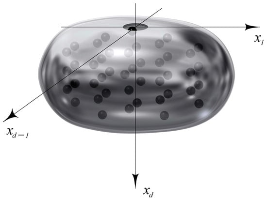
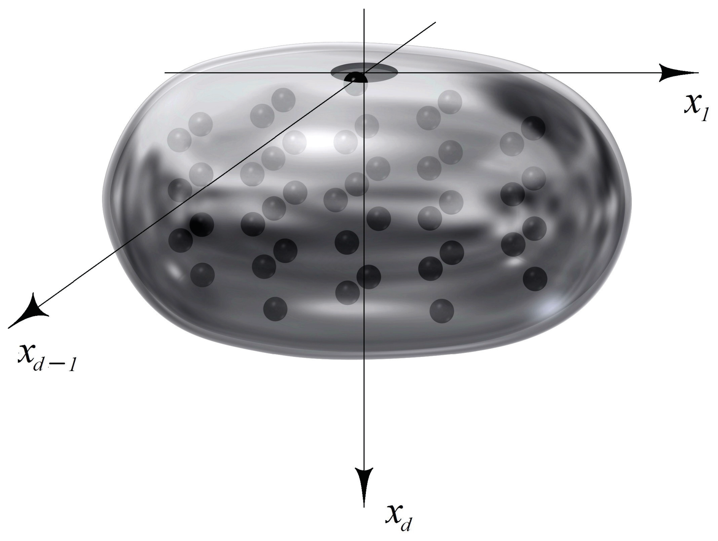
Here, and in what follows, we do not explicitly indicate the dependence on $\delta$, unless it leads to an ambiguity. In essence, we have a perforation “in a bag with a small hole”. According to the above construction, the boundary $\partial {\mathrm{\Omega }}_{+}^{\epsilon }$ consists of ${\mathrm{\Gamma }}_{\delta \left(\epsilon \right)}$ and the boundary of the inclusions $S_{\epsilon }\subset \mathrm{\Omega }$, $S_{\epsilon }=\left(\partial {\mathrm{\Omega }}_{+}^{\epsilon }\right)\cap \mathrm{\Omega }$ (see Figure 1).

Figure 1. Helmholtz resonator with micro-inhomogeneous structure.

We also use the notation

$${\mathrm{\Omega }}^{\epsilon }=\mathrm{\Omega }\setminus \left(\bigcup _{\mathbf{j}\in J^{\epsilon }}{Q}_{\mathbf{j}}^{\epsilon }\right).$$

Let us consider the following boundary value problem in an unbounded domain ${\mathrm{\Omega }}_{+}^{\epsilon }$:

$$\left\{\begin{array}{c}-\Delta u_{\epsilon }=k^2{u}_{\epsilon }+F\left(x\right)\mathrm{in}{\mathrm{\Omega }}_{+}^{\epsilon },\hfill \\ {\displaystyle \frac{\partial u_{\epsilon }}{\partial \nu }}+p\left({\displaystyle \frac{x}{\epsilon }}\right)u_{\epsilon }+\epsilon q\left({\displaystyle \frac{x}{\epsilon }}\right)u_{\epsilon }=0\mathrm{on}{S}_{\epsilon },\hfill \\ u_{\epsilon }=0\mathrm{on}{\mathrm{\Gamma }}_{\delta \left(\epsilon \right)},\hfill \end{array}\right.$$

(1)

$$u_{\epsilon }=O\left(r^{\frac{1-d}{2}}\right),{\displaystyle \frac{\partial u_{\epsilon }}{\partial r}}-\mathrm{i}k{u}_{\epsilon }=o\left(r^{\frac{1-d}{2}}\right)\mathrm{as}r\to \infty ,$$

(2)

where $\nu$ is the unit outward normal vector to the boundary of the inclusions, $r=\left|x\right|$, $k>0$, and F is a compactly supported function from $L_2\left({\mathbb{R}}^d\right)$. In what follows, we assume that the functions $p\left(\xi \right)$ and $q\left(\xi \right)$ are 1-periodic in $\xi \in {\mathbb{R}}^d$, $p(·),q(·)\in L_{\infty }\left(S\right)$, and

$${\displaystyle {⟨p(·)⟩\phantom{(}}_S=0,\mathrm{where}{⟨·⟩\phantom{(}}_S:=\underset{S}{\int }·d\sigma .}$$

(3)

Let $M\left(\xi \right)$ and $N_i\left(\xi \right)$, $i=1,\dots ,d$, be the ${[0,1)}^d$-periodic solutions of the boundary value problems

$$\left\{\begin{array}{c}{\Delta }_{\xi \xi }M\left(\xi \right)=0,\xi \in \square \setminus Q,\hfill \\ {\displaystyle \frac{\partial M\left(\xi \right)}{\partial {\nu }_{\xi }}}=-p\left(\xi \right),\xi \in S,\hfill \end{array}\right.$$

(4)

$$\left\{\begin{array}{c}{\Delta }_{\xi \xi }{N}_i\left(\xi \right)=0,\xi \in \square \setminus Q,\hfill \\ {\displaystyle \frac{\partial N_i\left(\xi \right)}{\partial {\nu }_{\xi }}}=-{\nu }_i,\xi \in S,\hfill \end{array}\right.$$

(5)

where, as before, $\nu$ is the unit outer normal vector to S. Since ${⟨{\nu }_j(·)⟩}_S=0$, $j=1,\dots ,d$, and due to (3), the compatibility condition for problems (4) and (5) is satisfied. Note that the functions $M\left(\xi \right)$ and $N_i\left(\xi \right)$ are defined up to an additive constant. To fix the choice of these constants, we impose the normalization conditions

$${⟨M⟩\phantom{(}}_{\square \setminus Q}={⟨N_i⟩\phantom{(}}_{\square \setminus Q}=0\forall i=1,\dots ,d,$$

and assume in the rest of the paper that these conditions are fulfilled.

Let us denote

$$\mathcal{L}u:=-{\displaystyle \frac{1}{|\square \setminus Q|}}\left({\widehat{a}}_{kj}{\displaystyle \frac{{\partial }^{2}u\left(x\right)}{\partial x_k\partial x_j}}-{⟨q⟩\phantom{(}}_{S}u\left(x\right)+mu\left(x\right)\right),$$

where

$${\widehat{a}}_{ik}:=\underset{\square \setminus Q}{\int }\left({\displaystyle \frac{\partial N_k\left(\xi \right)}{\partial {\xi }_i}}+{\delta }_{ik}\right)d\xi ,m:=-{⟨pM⟩\phantom{(}}_S.$$

(6)

From now on, we assume summation over repeating indices. It is known that the matrix $\widehat{a}$ is positive definite; see, for instance, [2].

According to [25], under the above assumptions on the geometry of the domain ${\mathrm{\Omega }}^{\epsilon }$, there exists an extension operator ${\mathcal{Z}}^{\epsilon }:H^1\left({\mathrm{\Omega }}^{\epsilon }\right)\mapsto H^1\left(\mathrm{\Omega }\right)$ such that for any $u\in H^1\left({\mathrm{\Omega }}^{\epsilon }\right)$

$$\parallel {\mathcal{Z}}^{\epsilon }{u\parallel }_{L_2\left(\mathrm{\Omega }\right)}⩽{C\parallel u\parallel }_{L_2\left({\mathrm{\Omega }}^{\epsilon }\right)},\parallel \nabla \left({\mathcal{Z}}^{\epsilon }u\right){\parallel }_{L_2\left(\mathrm{\Omega }\right)}⩽C{\parallel \nabla u\parallel }_{L_2\left({\mathrm{\Omega }}^{\epsilon }\right)},$$

with a constant C that does not depend on $\epsilon$. For the sake of brevity, we denote the extended function by the same symbol.

Our first goal is to prove the following statement.

Theorem 1.

Let f and $\tilde{f}$ be the restrictions of F to Ω and ${\mathbb{R}}^d\setminus \mathrm{\Omega }$, respectively, and assume that $\lambda =k^2$ is not an eigenvalue of the Dirichlet problem for $\mathcal{L}$ in Ω. Then, as $\epsilon \to 0$, the solution of the boundary value problem (1), (2) converges strongly in $L_{2,\mathrm{loc}}\left({\mathbb{R}}^d\right)$ to the function

$$\begin{array}{c}\hfill u\left(x\right)=\left\{\begin{array}{c}{u}_0\left(x\right),x\in \mathrm{\Omega },\hfill \\ {\tilde{u}}_0\left(x\right),x\in {\mathbb{R}}^d\setminus \overline{\mathrm{\Omega }},\hfill \end{array}\right.\end{array}$$

where $u_0\left(x\right)$ is the solution to the boundary value problem

$$\begin{array}{cc}& \left\{\begin{array}{c}\mathcal{L}{u}_0=k^2{u}_0+f,x\in \mathrm{\Omega },\hfill \\ u_0=0,x\in {\mathrm{\Gamma }}_0,\hfill \end{array}\right.\hfill \end{array}$$

(7)

and ${\tilde{u}}_0\left(x\right)$ is a solution of the boundary value problem

$$\begin{array}{c}\hfill \left\{\begin{array}{c}-\Delta {\tilde{u}}_0=k^2{\tilde{u}}_0+\tilde{f},x\in {\mathbb{R}}^d\setminus \overline{\mathrm{\Omega }},\hfill \\ {\tilde{u}}_0=0,x\in {\mathrm{\Gamma }}_0\hfill \end{array}\right.\end{array}$$

(8)

with the radiation conditions

$${\tilde{u}}_0=O\left(r^{\frac{1-d}{2}}\right),{\displaystyle \frac{\partial {\tilde{u}}_0}{\partial r}}-\mathrm{i}k{\tilde{u}}_0=o\left(r^{\frac{1-d}{2}}\right)\mathrm{as}r\to \infty .$$

(9)

If $\lambda =k_0^2$ is an eigenvalue of the Dirichlet problem for the operator $\mathcal{L}$ in Ω, then there exists a pole ${\tau }_{\epsilon }$ of the analytic continuation of a solution of the boundary value problem (1), (2), which lies in the half-plane $\mathrm{Im}k<0$ and converges to $k_0$ as $\epsilon \to 0$.

The concept of analytic continuation in Helmholtz-type problems is well known. For the reader’s convenience, all necessary definitions are given below.

The proof of Theorem 1 relies on the results on homogenization of an auxiliary problem in a bounded domain. These results are of independent interest.

Let $\tilde{\mathrm{\Omega }}$ be a smooth bounded domain in ${\mathbb{R}}^d$ such that $\overline{\mathrm{\Omega }}\subset \tilde{\mathrm{\Omega }}$. We denote $\tilde{\mathrm{\Gamma }}=\partial \tilde{\mathrm{\Omega }}$, ${\tilde{\mathrm{\Omega }}}^{\epsilon }=\tilde{\mathrm{\Omega }}\cap {\mathrm{\Omega }}_{+}^{\epsilon }$, ${\tilde{\mathrm{\Gamma }}}_{\epsilon }=\tilde{\mathrm{\Gamma }}\cup {\mathrm{\Gamma }}_{\delta \left(\epsilon \right)}$ and, for an arbitrary function $F\in L_2\left(\tilde{\mathrm{\Omega }}\right)$, use the notation f and $\tilde{f}$ for the restrictions of F to $\mathrm{\Omega }$ and $\tilde{\mathrm{\Omega }}\setminus \overline{\mathrm{\Omega }}$, respectively.

Consider the auxiliary problem

$$\left\{\begin{array}{c}-\Delta u_{\epsilon }=F\left(x\right)\mathrm{in}{\tilde{\mathrm{\Omega }}}^{\epsilon },\hfill \\ {\displaystyle \frac{\partial u_{\epsilon }}{\partial \nu }}+p\left({\displaystyle \frac{x}{\epsilon }}\right)u_{\epsilon }+\epsilon q\left({\displaystyle \frac{x}{\epsilon }}\right)u_{\epsilon }=0\mathrm{on}{S}_{\epsilon },\hfill \\ u_{\epsilon }=0\mathrm{on}{\tilde{\mathrm{\Gamma }}}_{\epsilon }.\hfill \end{array}\right.$$

(10)

Assuming that the homogeneous problem with $F=0$ has only a zero solution, we define ${\mathcal{L}}_{\epsilon }^{-1}$ as the bounded operator that associates $F\in L_2({\tilde{\mathrm{\Omega }}}^{\epsilon })$ with the solution of the boundary value problem (10) defined in $L_2({\tilde{\mathrm{\Omega }}}^{\epsilon })$. Then, assuming also that the homogenized problem

$$\begin{array}{cc}& \left\{\begin{array}{c}\mathcal{L}u=f,x\in \mathrm{\Omega },\hfill \\ u=0,x\in {\mathrm{\Gamma }}_0,\hfill \end{array}\right.\hfill \end{array}$$

(11)

is well posed, we denote its solution by $u_0\left(x\right)$. Letting ${\tilde{u}}_0\left(x\right)$ be the solution of the boundary value problem

$$\begin{array}{c}\hfill \left\{\begin{array}{c}-\Delta u=\tilde{f},x\in \tilde{\mathrm{\Omega }}\setminus \overline{\mathrm{\Omega }},\hfill \\ u=0,x\in {\mathrm{\Gamma }}_0\cup \tilde{\mathrm{\Gamma }};\hfill \end{array}\right.,\end{array}$$

(12)

we define the function

$$\begin{array}{c}\hfill u\left(x\right)=\left\{\begin{array}{c}{u}_0\left(x\right),x\in \mathrm{\Omega },\hfill \\ {\tilde{u}}_0\left(x\right),x\in \tilde{\mathrm{\Omega }}\setminus \overline{\mathrm{\Omega }},\hfill \end{array}\right.\end{array}$$

(13)

and denote by ${\mathcal{L}}_0^{-1}$ the operator that maps $F\in L_2\left(\tilde{\mathrm{\Omega }}\right)$ to the function introduced in (13); recall that f and $\tilde{f}$ are the restrictions of F to $\mathrm{\Omega }$ and $\tilde{\mathrm{\Omega }}\setminus \overline{\mathrm{\Omega }}$, respectively.

By ${\mathcal{L}}_{0,\epsilon }^{-1}$, we denote the operator that maps the function $F\in L_2(\widetilde{{\mathrm{\Omega }}^{\epsilon }})$ to the function $u_{0,\epsilon }:={\mathbf{1}}_{{\tilde{\mathrm{\Omega }}}^{\epsilon }}{\mathcal{L}}_0^{-1}\left({\mathbf{1}}_{{\tilde{\mathrm{\Omega }}}^{\epsilon }}F\right)$. Note that ${\mathcal{L}}_{0,\epsilon }^{-1}$ and ${\mathcal{L}}_{\epsilon }^{-1}$ are operators in $L_2({\tilde{\mathrm{\Omega }}}^{\epsilon })$.

Theorem 2.

Let $\lambda =0$ not be an eigenvalue of the Dirichlet problem for the operator $\mathcal{L}$ in Ω. Then for all sufficiently small $\epsilon >0$:

(a) 

The problems (10)–(12) are uniquely solvable;

(b) 

The following estimate uniform in ε holds:

$${∥u_{\epsilon }∥}_{H^1\left({\tilde{\mathrm{\Omega }}}^{\epsilon }\right)}⩽C{∥F∥}_{L_2\left({\tilde{\mathrm{\Omega }}}^{\epsilon }\right)};$$

(14)

(c) 

For any $F\in L_2({\tilde{\mathrm{\Omega }}}^{\epsilon })$, the solution $u^{\epsilon }$ of problem (10) converges to the function $u(·)$ defined in (13). Moreover, the convergence in the operator norm holds:

$$\parallel {\mathcal{L}}_{0,\epsilon }^{-1}-{\mathcal{L}}_{\epsilon }^{-1}{\parallel }_{\mathcal{B}\left(L_2\left({\tilde{\mathrm{\Omega }}}^{\epsilon }\right)\right)}⟶0,\mathrm{as}\epsilon \to 0;$$

(15)

Here, $\mathcal{B}(L_2({\tilde{\mathrm{\Omega }}}^{\epsilon }))$ is the Banach space of linear bounded operators in $L_2({\tilde{\mathrm{\Omega }}}^{\epsilon })$.

(d) 

For any region ${\mathrm{\Omega }}^{\prime }\subset \tilde{\mathrm{\Omega }}\setminus \overline{\mathrm{\Omega }}$ separated from ${\mathrm{\Gamma }}_0$, there is a strong convergence of $u_{\epsilon }\to {\tilde{u}}_0$ in $H^2\left({\mathrm{\Omega }}^{\prime }\right)$.

The proof of this Theorem is given below in Section 7.

Concerning operator estimates, see also [27,28,29].

3. Construction of Analytical Continuation

The construction of analytic continuation of solutions of boundary value problems (1), (2) and (8), (9) given in this section is fairly standard (see, for example, [24,27]). Let $X\left(D\right)$ be a Banach space of functions $u:D\mapsto \mathbb{R}$ defined on some set $D\subset {\mathbb{R}}^d$ (for example, $X\left(D\right)=L_2\left(D\right)$). Then $X_{\mathrm{loc}}\left(D\right)\stackrel{\mathrm{def}}{=}\{u:u\in X(D\cap S\left(R\right))\forall R\}$, where $S\left(R\right)$ is an open d-dimensional ball of radius R centered at the origin. The notation $\mathcal{B}(X,Y)$ stands for the Banach space of bounded linear operators from a Banach space X to a Banach space Y, $\mathcal{B}\left(X\right)\stackrel{\mathrm{def}}{=}\mathcal{B}(X,X)$, and $\mathcal{B}(Y,X_{\mathrm{loc}}\left(D\right))$ is the space of linear operators $\mathcal{A}:Y\to X_{\mathrm{loc}}\left(D\right)$ such that $\mathcal{A}\in \mathcal{B}(Y,X(D\cap S\left(R\right)\left)\right)$ for any $R>0$. By ${\mathcal{B}}^h(X,Y)$ (or ${\mathcal{B}}^m(X,Y)$), we denote the set of holomorphic (meromorphic) operator-valued functions with values in $\mathcal{B}(X,Y)$; that is, ${\mathcal{B}}^h(X,Y)=\{\mathcal{A}(·):\mathbb{C}\mapsto \mathcal{B}(X,Y):\mathcal{A}(·)\mathrm{is}\mathrm{holomorphic}\}$. Then, we set ${\mathcal{B}}^h(X,X)\stackrel{\mathrm{def}}{=}{\mathcal{B}}^h\left(X\right)$ ${\mathcal{B}}^h(X,Y_{\mathrm{loc}}\left(D\right))\stackrel{\mathrm{def}}{=}\{\mathcal{A}:\mathcal{A}\in {\mathcal{B}}^h(X,Y(D\cap S\left(R\right)))\forall R>0\}$.

Let L be a positive number such that $\overline{\mathrm{\Omega }}\subset S(L/3)$. With this choice of L, we can set $\tilde{\mathrm{\Omega }}=S\left(L\right)$; this value of L is fixed in what follows. Consider a family of boundary value problems in bounded domains ${\tilde{\mathrm{\Omega }}}^{\epsilon }$:

$$\left\{\begin{array}{c}\Delta u_{\epsilon }=\Delta w\mathrm{in}{\tilde{\mathrm{\Omega }}}^{\epsilon },\hfill \\ {\displaystyle \frac{\partial u_{\epsilon }}{\partial \nu }}+p\left({\displaystyle \frac{x}{\epsilon }}\right)u_{\epsilon }+\epsilon q\left({\displaystyle \frac{x}{\epsilon }}\right)u_{\epsilon }=0\mathrm{on}{S}_{\epsilon },\hfill \\ u_{\epsilon }=0\mathrm{on}{\mathrm{\Gamma }}_{\delta \left(\epsilon \right)},u_{\epsilon }=w\mathrm{on}\tilde{\mathrm{\Gamma }},\hfill \end{array}\right.$$

(16)

where $w\in H^2(\tilde{\mathrm{\Omega }})$. Denote by ${\sigma }_{\epsilon }$ the operator that maps $w\in H^2(\tilde{\mathrm{\Omega }})$ to the solution $u_{\epsilon }\in H^1({\tilde{\mathrm{\Omega }}}^{\epsilon })$ of problem (16). Similarly, ${\sigma }_0$ stands for the operator that maps $w\in H^2(\tilde{\mathrm{\Omega }})$ to the pair of solutions $u_0\in H^2(\mathrm{\Omega })$ and ${\tilde{u}}_0\in H^2(\tilde{\mathrm{\Omega }}\setminus \overline{\mathrm{\Omega }})$ of the following boundary value problems:

$$\begin{array}{c}\hfill \left\{\begin{array}{c}\mathcal{L}{u}_0=\mathcal{L}w,x\in \mathrm{\Omega },\hfill \\ u_0=0,x\in \mathrm{\Gamma },\hfill \end{array}\right.\end{array}$$

(17)

and

$$\begin{array}{c}\hfill \left\{\begin{array}{c}\Delta {\tilde{u}}_0=\Delta w,x\in \tilde{\mathrm{\Omega }}\setminus \overline{\mathrm{\Omega }},\hfill \\ {\tilde{u}}_0=0,x\in \mathrm{\Gamma },{\tilde{u}}_0=w,x\in \tilde{\mathrm{\Gamma }}.\hfill \end{array}\right.\end{array}$$

(18)

Suppose that $g\in L_2(\tilde{\mathrm{\Omega }})$. Define

$${(\Delta +k^2)}^{-1}g\stackrel{\mathrm{def}}{=}\underset{\tilde{\mathrm{\Omega }}}{\int }G(|x-y|;k)g(y)dy,x\in {\mathbb{R}}^d,$$

Here, G is the fundamental solution of the Helmholtz equation in ${\mathbb{R}}^d$ for $k^2<0$ and its analytic continuation for other $k\in \tilde{\mathbb{C}}$, where the symbol $\tilde{\mathbb{C}}$ stands for the complex plane for odd d and for the complex plane with a cut along the non-positive real half-axis for even d. In what follows, we use the same notation for a function from $L_2(\tilde{\mathrm{\Omega }})$ ($L_2({\tilde{\mathrm{\Omega }}}^{\epsilon })$) and its continuation by zero outside $\tilde{\mathrm{\Omega }}$ (outside ${\tilde{\mathrm{\Omega }}}^{\epsilon }$); notice that the extended function is an element of $L_2({\mathbb{R}}^d)$. Also, for consistency of formulations, we introduce the notation

$${\tilde{\mathrm{\Omega }}}^0:=\tilde{\mathrm{\Omega }},{\mathrm{\Omega }}_{+}^0:={\mathbb{R}}^d,$$

and use the index $\mathbf{s}$, which takes the value either 0 or $\epsilon$. As a consequence of the definition of ${(\Delta +k^2)}^{-1}$ we have:

Lemma 1.

For $k\in \tilde{\mathbb{C}}$, the operator ${(\Delta +k^2)}^{-1}$ belongs to the space ${\mathcal{B}}^h(L_2({\tilde{\mathrm{\Omega }}}^{\mathbf{s}}),H_{\mathrm{loc}}^2({\mathbb{R}}^d))$, and if $g\in L_2(\tilde{\mathrm{\Omega }})$, then the function $U={(\Delta +k^2)}^{-1}g$ is a solution of the equation $(\Delta +k^2)U=g$ in ${\mathbb{R}}^d$, satisfying, for $k>0$, the radiation condition of the form

$$U=O\left(r^{\frac{1-d}{2}}\right),{\displaystyle \frac{\partial U}{\partial r}}-\mathrm{i}kU=o\left(r^{\frac{1-d}{2}}\right),r\to \infty .$$

Next, let $p_L$ be the restriction operator to $S(L)$ (recall that $S(L)=\tilde{\mathrm{\Omega }}$) and $\chi (t)$ be a smooth cuttoff function equal to one for $t<1/3$ and zero for $t>2/3$,

$$\begin{array}{cc}\hfill A_{\mathbf{s}}(k)\stackrel{\mathrm{def}}{=}& \left(1+\chi \left({\displaystyle \frac{r}{L}}\right)\left({\sigma }_{\mathbf{s}}{p}_L-1\right)\right){(\Delta +k^2)}^{-1},\hfill \\ \hfill T_{\mathbf{s}}(k)g\stackrel{\mathrm{def}}{=}& (\left(\Delta +k^2\right)\left(\chi \left({\displaystyle \frac{r}{L}}\right)\right)\left(\left(1-{\sigma }_{\mathbf{s}}{p}_L\right){\left(\Delta +k^2\right)}^{-1}\right)\hfill \\ \hfill & +2{\displaystyle \sum _{i=1}^d}{\displaystyle \frac{\partial }{\partial x_i}}\left(\chi \left({\displaystyle \frac{r}{L}}\right)\right){\displaystyle \frac{\partial }{\partial x_i}}\left(\left(1-{\sigma }_{\mathbf{s}}{p}_L\right){\left(\Delta +k^2\right)}^{-1}\right))g.\hfill \end{array}$$

From the definition of $T_{\mathbf{s}}(k)$, it follows that for $g\in L_2({\tilde{\mathrm{\Omega }}}^{\mathbf{s}})$, we have $T_{\mathbf{s}}(k)g\in L_2({\mathbb{R}}^d)$ and $\mathrm{supp}{T}_{\mathbf{s}}(k)g\subset \overline{{\tilde{\mathrm{\Omega }}}^{\mathbf{s}}}$. Therefore, the mappings $T_{\mathbf{s}}(k)$ and $B_{\mathbf{s}}(k)=I-T_{\mathbf{s}}(k)$, where I is the identity operator, can be regarded as operators in $\mathcal{B}(L_2({\tilde{\mathrm{\Omega }}}^{\mathbf{s}}))$. In this interpretation, the following assertion follows from the definition of the operators $T_{\mathbf{s}}$ and $A_{\mathbf{s}}$, items (a) and (b) of Theorem 2 and Lemma 1, according to [26].

Lemma 2.

For any fixed $\mathbf{s}⩾0$, we have:

(a) 

$A_{\mathbf{s}}(k)\in {\mathcal{B}}^h\left(L_2({\tilde{\mathrm{\Omega }}}^{\mathbf{s}}),H_{\mathrm{loc}}^1({\mathrm{\Omega }}_{+}^{\mathbf{s}})\right)$, $T_{\mathbf{s}}(k)\in {\mathcal{B}}^h\left(L_2({\tilde{\mathrm{\Omega }}}^{\mathbf{s}})\right)$ at $k\in \tilde{\mathbb{C}}$;

(b) 

$T_{\mathbf{s}}(k)$ is a compact operator in $L_2({\tilde{\mathrm{\Omega }}}^{\mathbf{s}})$;

(c) 

If $g_{\epsilon }\in L_2({\tilde{\mathrm{\Omega }}}^{\epsilon })$, then the function $u_{\epsilon }=A_{\epsilon }(k)g_{\epsilon }$ satisfies (1) for $F=-(I-T_{\epsilon }(k))g_{\epsilon }$; for $g_0\in L_2({\tilde{\mathrm{\Omega }}}^0)$, the restriction $u_0$ of $A_0(k)g_0$ to Ω satisfies (7), where f is the restriction of $-(I-T_0(k))g_0$ to Ω. The restriction ${\tilde{u}}_0$ of $A_0(k)g_0$ on ${\mathbb{R}}^d\setminus \overline{\mathrm{\Omega }}$ satisfies (8), where $\tilde{f}$ is the restriction of the function $-(I-T_0(k))g_0$ on $\tilde{\mathrm{\Omega }}\setminus \overline{\mathrm{\Omega }}$;

(d) 

i=if $k>0$, then the functions $A_{\epsilon }(k)g_{\epsilon }$ and $A_0(k)g_0$ satisfy the radiation conditions (2) and (9), respectively.

The square root of an eigenvalue of the Dirichlet problem for the operator $\mathcal{L}$ in $\mathrm{\Omega }$ is called an eigenfrequency of the Dirichlet problem; the set of such eigenfrequencies is denoted by $\mathrm{\Sigma }$.

Lemma 3.

If $\mathrm{Im}k>0$ or $k>0$, then a solution of the boundary value problem (1), (2) and (8), (9) is unique in $H_{\mathrm{loc}}^1({\mathrm{\Omega }}_{+}^{\epsilon })$ and in $H_{\mathrm{loc}}^1({\mathbb{R}}^d\setminus \overline{\mathrm{\Omega }})$, respectively. If $k\notin \mathrm{\Sigma }$, then a solution of the boundary value problem (7) exists and is unique in $H^1(\mathrm{\Omega })$.

The validity of this statement was substantiated, for example, in the works [26,27].

Lemma 4.

If $g\ne 0$ and $g\in L_2({\tilde{\mathrm{\Omega }}}^{\mathbf{s}})$, then $A_{\mathbf{s}}(k)g\ne 0$.

The proof of this statement is completely identical to the proof of Lemma 2.2 in [27] and Lemma 3.3 in [26].

Lemmata 3 and 4 and the compactness of the operator $T_{\mathbf{s}}(k)$ yield

Lemma 5.

If $\mathrm{Im}k>0$ or $k>0$ and $k\notin \mathrm{\Sigma }$, then ${\left(B_{\mathbf{s}}\right)}^{-1}(k)\in \mathcal{B}({\tilde{\mathrm{\Omega }}}^{\mathbf{s}})$.

The next Lemma is proved in [24].

Lemma 6.

Let D be a connected domain in the complex plane, $T(k)$ ($k\in D$) be a holomorphic family of compact operators in a Banach space $\mathcal{X}$, and there exists $k_{*}\in D$ such that ${(I-T(k_{*}))}^{-1}\in \mathcal{B}(\mathcal{X})$. Then ${(I-T(k))}^{-1}$ is a meromorphic function in D with values in $\mathcal{B}(\mathcal{X})$.

As a consequence of Lemmata 5 and 6 we obtain

Lemma 7.

${\left(B_{\mathbf{s}}\right)}^{-1}(k)\in {\mathcal{B}}^m(L_2({\tilde{\mathrm{\Omega }}}^{\mathbf{s}}))$ in $\tilde{\mathbb{C}}$.

Denote

$${\mathcal{A}}_{\mathbf{s}}(k)\stackrel{\mathrm{def}}{=}{A}_{\mathbf{s}}(k){\left(B_{\mathbf{s}}\right)}^{-1}(k).$$

Theorem 3.

For $k\in \tilde{\mathbb{C}}$,

(a) 

${\mathcal{A}}_{\mathbf{s}}(k)\in {\mathcal{B}}^m\left(L_2({\tilde{\mathrm{\Omega }}}^{\mathbf{s}}),H_{\mathrm{loc}}^1({\mathrm{\Omega }}^{\mathbf{s}})\right)$;

(b) 

The function $u_{\epsilon }=-{\mathcal{A}}_{\epsilon }(k)F$ satisfies (1); the restriction $u_0$$({\tilde{u}}_0)$ of the function $-{\mathcal{A}}_0(k)F$ to Ω (to ${\mathbb{R}}^d\setminus \overline{\mathrm{\Omega }}$) satisfies (7) and (8), where f ($\tilde{f}$) is the restriction of F to Ω (to $\tilde{\mathrm{\Omega }}\setminus \overline{\mathrm{\Omega }}$); and for $\mathrm{Im}k>0$ or $k>0$ the functions $u_{\epsilon }$ and ${\tilde{u}}_0$ satisfy the radiation conditions (2) and (9);

(c) 

The sets of poles of the operators ${\mathcal{A}}_{\mathbf{s}}(k)$ and ${\left(B_{\mathbf{s}}(k)\right)}^{-1}$ coincide;

(d) 

If $\tilde{\mathrm{\Omega }}=S(L)$ and $\mathrm{supp}F\subset S(T)$, then the function ${\mathcal{A}}_{\mathbf{s}}(k)F$, $\mathbf{s}=\epsilon ,0$, does not depend on $L⩾T$;

(e) 

The set of poles of the operator ${\mathcal{A}}_{\epsilon }(k)$ does not depend on L.

Proof. 

Assertions (a) and (b) follow from Lemmata 2 and 7. Assertion (c) follows from Lemma 4 and the definition of the operator ${\mathcal{A}}_{\epsilon }(k)$. Assertion (d) follows from Lemma 3 and the uniqueness of the analytic continuation. Let us show that assertion (d) holds true for $\epsilon >0$. Denote by ${\mathcal{A}}_{\epsilon ,t}$ the operator ${\mathcal{A}}_{\epsilon }$ defined for $L=t$. Let $a>b$. Obviously, the set of poles of ${\mathcal{A}}_{\epsilon ,b}$ is a subset of the poles of ${\mathcal{A}}_{\epsilon ,a}$. Let us justify the inverse inclusion. Assume that $\mathrm{supp}F\subset S(a)$ and denote

$$W=-(1-\chi (r{b}^{-1})){(\Delta +k^2)}^{-1}F.$$

Since $\mathrm{supp}(F-(\Delta +k^2)W)\subset \overline{S(b)}$, by (b), the solution of the perturbed problem (1) and (2) and its analytic continuation can be represented in any of the following forms:

$$u_{\epsilon }=-{\mathcal{A}}_{\epsilon ,a}(k)F,u_{\epsilon }=-{\mathcal{A}}_{\epsilon ,a}(k)(F-(\Delta +k^2)W)+W.$$

Since the function W is holomorphic, the set of poles of ${\mathcal{A}}_{\epsilon ,a}$ is a subset of the poles of ${\mathcal{A}}_{\epsilon ,b}$. The case $\mathbf{s}=0$ is considered similarly. The theorem is proved. □

4. Proof of Theorem 1

Just as in the case of the operator ${\mathcal{L}}_{\epsilon }^{-1}$, we assume that the operators ${\sigma }_{\epsilon }$, $T_{\epsilon }(k)$, $A_{\epsilon }(k)$, and ${\mathcal{A}}_{\epsilon }(k)$ are extended by zero into $\tilde{\mathrm{\Omega }}\setminus \overline{{\tilde{\mathrm{\Omega }}}^{\epsilon }}$. Moreover, we define the domain of definition for $T_{\epsilon }(k)$ as $L_2(\tilde{\mathrm{\Omega }})$, narrowing the function from $L_2(\tilde{\mathrm{\Omega }})$ to ${\tilde{\mathrm{\Omega }}}^{\epsilon }$ before acting on it with the operator $T_{\epsilon }(k)$. Then, by virtue of the definition of the operators $A_{\epsilon }(k)$ and ${\mathcal{A}}_{\epsilon }(k)$, their domain of definition is also $L_2(\tilde{\mathrm{\Omega }})$.

From the definition of the operators ${\sigma }_{\mathbf{s}}$ and $T_{\mathbf{s}}(k)$ and assertions (a)–(c) of Theorem 2, it follows

Lemma 8.

$\parallel T_{\epsilon }(k)-T_0{(k)\parallel }_{\mathcal{B}(L_2(\tilde{\mathrm{\Omega }}))}\underset{\epsilon \to 0}{\to }0$.

In [24], the following statement is proved.

Lemma 9.

Let D be a connected domain in the complex plane and $T(k,\mu )$ be a family of compact operators in a Banach space $\mathcal{X}$ defined for $k\in D$ and $\mu \in [0,{\mu }_0]$ such that it is holomorphic in k for any μ and continuous in $D\times [0,{\mu }_0]$ with respect to the norm of $\mathcal{B}(\mathcal{X})$. Further, suppose that there exists $k_0\in D$ such that ${(I-T(k_0,\mu ))}^{-1}\in \mathcal{B}(\mathcal{X})$ for any $\mu \in (0,{\mu }_0)$. Then:

(a) 

${(I-T(k,\mu ))}^{-1}$ (for any μ) is a meromorphic function in D with values in $\mathcal{B}(\mathcal{X})$;

(b) 

If $k_{*}$ is not a pole of ${(I-T(k,{\mu }_{*}))}^{-1}$, the operator-valued function ${(I-T(k,\mu ))}^{-1}$ is norm-continuous in a neighborhood of $(k_{*},{\mu }_{*})$;

(c) 

The poles of ${(I-T(k,\mu ))}^{-1}$ depend on μ continuously.

We denote by ${\mathrm{\Sigma }}_{\mathbf{s}}$ the set of poles of the operator ${\mathcal{A}}_{\mathbf{s}}$. By virtue of Lemmata 2, 7 and 8, the family $T_{\mathbf{s}}(k)$ satisfies the conditions of Lemma 9. Therefore, taking into account assertion (c) of Theorem 3, we arrive at the following Lemma.

Lemma 10.

If K is an arbitrary compact set in $\tilde{\mathbb{C}}$ such that $K\cap {\mathrm{\Sigma }}_0=\varnothing$, then ${\left(B_{\epsilon }(k)\right)}^{-1}\underset{\epsilon \to 0}{\to }{\left(B_0(k)\right)}^{-1}$ in the norm of $\mathcal{B}(L_2(\tilde{\mathrm{\Omega }}))$ uniformly in $k\in K$. If ${\tau }_0\in {\mathrm{\Sigma }}_0$, then there exists a pole ${\tau }_{\epsilon }\in {\mathrm{\Sigma }}_{\epsilon }$ converging to ${\tau }_0$ as $\epsilon \to 0$.

From the definition of the operators ${\sigma }_{\mathbf{s}}$ and ${\mathcal{A}}_{\mathbf{s}}(k)$ and statements (a)–(d) of Theorem 2 and Lemma 10, we obtain the following statement:

Theorem 4.

If K is an arbitrary compact set in $\tilde{\mathbb{C}}$ such that $K\cap {\mathrm{\Sigma }}_0=\varnothing$, then ${\mathcal{A}}_{\epsilon }(k)\underset{\epsilon \to 0}{⟶}{\mathcal{A}}_0(k)$ in the norm of $\mathcal{B}(L_2(\tilde{\mathrm{\Omega }}),L_{2,\mathrm{loc}}({\mathbb{R}}^d))$ uniformly in $k\in K$. If ${\tau }_0\in {\mathrm{\Sigma }}_0$, then there exists a pole ${\tau }_{\epsilon }\in {\mathrm{\Sigma }}_{\epsilon }$ converging to ${\tau }_0$ as $\epsilon \to 0$.

Theorem 1 is a direct consequence of Theorems 3 and 4. The existence of poles with small imaginary parts follows from the fact that $\mathrm{\Sigma }\subset {\mathrm{\Sigma }}_0$.

5. A Priori Estimates and the Homogenized Operator

Let us consider a model problem in the area ${\mathrm{\Omega }}^{\epsilon }=\mathrm{\Omega }\setminus \left(\bigcup _{\mathbf{j}\in J^{\epsilon }}{Q}_{\mathbf{j}}^{\epsilon }\right)$ of the form

$$\left\{\begin{array}{c}-\Delta u_{\epsilon }=f(x)\mathrm{in}{\mathrm{\Omega }}^{\epsilon },\hfill \\ {\displaystyle \frac{\partial u_{\epsilon }}{\partial \nu }}+p({\displaystyle \frac{x}{\epsilon }})u_{\epsilon }+\epsilon q({\displaystyle \frac{x}{\epsilon }})u_{\epsilon }=0\mathrm{on}{S}_{\epsilon },\hfill \\ u_{\epsilon }=0\mathrm{on}{\mathrm{\Gamma }}_0\hfill \end{array}\right.$$

(19)

Let us begin with the proof of the a priori estimate, which we obtain for a more general problem of the form

$$\left\{\begin{array}{c}-\Delta u_{\epsilon }=f(x)\mathrm{in}{\mathrm{\Omega }}^{\epsilon },\hfill \\ {\displaystyle \frac{\partial u_{\epsilon }}{\partial \nu }}+p({\displaystyle \frac{x}{\epsilon }})u_{\epsilon }+\epsilon q({\displaystyle \frac{x}{\epsilon }})u_{\epsilon }=g(x)\mathrm{on}{S}_{\epsilon },\hfill \\ u_{\epsilon }=0\mathrm{on}{\mathrm{\Gamma }}_0,\hfill \end{array}\right.$$

(20)

in which $f\in L_2(\mathrm{\Omega })$ and $g\in L_2(S_{\epsilon })$.

Lemma 11.

Let $\lambda =0$ not be an eigenvalue of the operator of problem (11); i.e., problem (11) has no non-zero solutions. Then there exists a constant $C>0$ such that for all sufficiently small $\epsilon >0$ and for all $f\in L_2(\mathrm{\Omega })$ and $g\in L_2(S_{\epsilon })$, the solution of problem (20) satisfies the estimate

$$\parallel u_{\epsilon }{\parallel }_{H^1({\mathrm{\Omega }}^{\epsilon })}⩽C({\parallel f\parallel }_{L_2({\mathrm{\Omega }}^{\epsilon })}+{\epsilon }^{-\frac{1}{2}}{\parallel g\parallel }_{L_2(S_{\epsilon })}),$$

(21)

with a constant C that does not depend on ε.

Proof. 

Suppose that the statement of the above lemma is not satisfied. Then there exists a sequence ${\epsilon }_k$ tending to zero as $k\to \infty$, and sequences of functions $f^{{\epsilon }_k}$ and $g^{{\epsilon }_k}$ such that

$$\underset{k\to \infty }{\lim }\parallel f^{{\epsilon }_k}{\parallel }_{L_2({\mathrm{\Omega }}^{{\epsilon }_k})}=0,\underset{k\to \infty }{\lim }{\epsilon }^{-{\displaystyle \frac{1}{2}}}\parallel g^{{\epsilon }_k}{\parallel }_{L_2(S_{\epsilon })}=0,\mathrm{and}{\parallel u_{{\epsilon }_k}\parallel }_{H^1({\mathrm{\Omega }}^{{\epsilon }_k})}=1.$$

In what follows, for convenience of notation, we omit the index k and write $\epsilon$ instead of ${\epsilon }_k$. Using the standard extension operator (see [25]), we can assume that $u_{\epsilon }$ is defined in the entire domain $\mathrm{\Omega }$, and $\parallel u_{\epsilon }{\parallel }_{H^1(\mathrm{\Omega })}⩽C_0$. Therefore, with respect to a subsequence, $u_{\epsilon }$ converges to some function $u_0\in H_0^1(\mathrm{\Omega })$ weakly in $H^1(\mathrm{\Omega })$ and in the norm of $L_2(\mathrm{\Omega })$. Choosing, if necessary, a subsequence, we can assume that $\parallel \nabla u_{\epsilon }{\parallel }_{L_2({\mathrm{\Omega }}^{\epsilon })}$ converges as $\epsilon \to 0$ to some constant $\kappa$. Since the Friedrichs inequality $\parallel u_{\epsilon }{\parallel }_{L_2({\mathrm{\Omega }}^{\epsilon })}⩽C{\parallel \nabla u_{\epsilon }\parallel }_{L_2({\mathrm{\Omega }}^{\epsilon })}$ holds uniformly in $\epsilon >0$, we conclude that $\kappa >0$. Multiplying the equation in (20) by ${\overline{u}}_{\epsilon }$ and integrating the resulting equality over the set ${\mathrm{\Omega }}^{\epsilon }$, after integrating by parts, we find:

$$\underset{{\mathrm{\Omega }}^{\epsilon }}{\int }|\nabla u_{\epsilon }{|}^{2}dx+\underset{S_{\epsilon }}{\int }p\left(\frac{x}{\epsilon }\right)|u_{\epsilon }{|}^{2}d\sigma +\epsilon \underset{S_{\epsilon }}{\int }q\left(\frac{x}{\epsilon }\right){|u_{\epsilon }|}^{2}d\sigma =\underset{{\mathrm{\Omega }}^{\epsilon }}{\int }{f}^{\epsilon }{\overline{u}}_{\epsilon }dx+\underset{S_{\epsilon }}{\int }{g}^{\epsilon }{\overline{u}}_{\epsilon }d\sigma .$$

If we assume that $u_0=0$, then passing here to the limit as $\epsilon \to 0$ and applying Lemma 18, we obtain the equality ${\kappa }^2=0$, which contradicts the inequality $\kappa >0$.

Now we choose an arbitrary test function $v\in C_0^{\infty }(\mathrm{\Omega })$, and define

$$v^{\epsilon }(x)=v(x)+\epsilon M\left({\displaystyle \frac{x}{\epsilon }}\right)v(x)+\epsilon N\left({\displaystyle \frac{x}{\epsilon }}\right)·\nabla v(x).$$

(22)

Multiplying the equation in (19) by ${\overline{v}}^{\epsilon }$ and integrating the resulting equality over ${\mathrm{\Omega }}^{\epsilon }$, after integrating by parts and passing to the limit as $\epsilon \to 0$, we conclude that $u_0$ is a solution to the problem $\mathcal{L}{u}_0=0$ in $\mathrm{\Omega }$, $u_0=0$ on $\partial \mathrm{\Omega }$. This equation is derived in exactly the same way as in the proof of Lemma 13 given below in this section, so we omit this proof here. Since the limit problem has only the trivial solution $u_0=0$, we obtain a contradiction. □

Lemma 12.

The functions $M(\xi )$ and $N_k(\xi )$ are connected by the following integral formula

$$\underset{\square \setminus Q}{\int }{\displaystyle \frac{\partial M}{\partial {\xi }_k}}d\xi -\underset{S}{\int }p{N}_{k}d\sigma =0.$$

Proof. 

The proof of this Lemma is given in [19]. □

Lemma 13.

Let $\lambda =0$ not be an eigenvalue of the operator of problem (11). Then for all $f\in L_2(\mathrm{\Omega })$, the solution $u_{\epsilon }$ of problem (19) converges as $\epsilon \to 0$ to the solution $u_0$ of the homogenized problem (11) in the space $L_2({\mathrm{\Omega }}^{\epsilon })$, i.e.,

$$\underset{\epsilon \to 0}{\lim }{\parallel u_{\epsilon }-u_0\parallel }_{L_2({\mathrm{\Omega }}^{\epsilon })}=0.$$

Proof. 

According to Lemma 11, the family of solutions $\left\{u_{\epsilon }\right\}$ is bounded in $H^1({\mathrm{\Omega }}^{\epsilon })$. Applying the extension operator to the functions $u_{\epsilon }$, as shown in [25], we can assume that $u_{\epsilon }$ is a bounded family in $H_0^1(\mathrm{\Omega })$. Therefore, by subsequence, the family $u_{\epsilon }$ converges as $\epsilon \to 0$ to some function $u_0\in H_0^1(\mathrm{\Omega })$. In the integral identity of problem (19), we choose the test function defined in (22), and after simple transformations, we obtain

$$\underset{{\mathrm{\Omega }}^{\epsilon }}{\int }\nabla u_{\epsilon }·\left[\nabla \overline{v}+\nabla N\left(\frac{x}{\epsilon }\right)\nabla \overline{v}+\nabla M\left(\frac{x}{\epsilon }\right)\overline{v}\right]dx-\underset{S_{\epsilon }}{\int }{u}_{\epsilon }p\left(\frac{x}{\epsilon }\right)[\overline{v}+\epsilon N\left(\frac{x}{\epsilon }\right)·\nabla \overline{v}+\epsilon M\left(\frac{x}{\epsilon }\right)\overline{v}]d\sigma$$

$$-\epsilon \underset{S_{\epsilon }}{\int }{u}_{\epsilon }q\left(\frac{x}{\epsilon }\right)\overline{v}d\sigma =\underset{{\mathrm{\Omega }}^{\epsilon }}{\int }f\overline{v}dx+o(1),$$

where $o(1)$ tends to zero as $\epsilon \to 0$. Integrating by parts one more time in the first term of this equality yields

$$-\underset{{\mathrm{\Omega }}^{\epsilon }}{\int }{u}_{\epsilon }\left[\Delta \overline{v}+\nabla N\left(\frac{x}{\epsilon }\right)·\nabla \nabla \overline{v}+\nabla M\left(\frac{x}{\epsilon }\right)\nabla \overline{v}\right]dx$$

$$-\underset{S_{\epsilon }}{\int }{u}_{\epsilon }p\left(\frac{x}{\epsilon }\right)[\epsilon N\left(\frac{x}{\epsilon }\right)·\nabla \overline{v}+\epsilon M\left(\frac{x}{\epsilon }\right)\overline{v}]d\sigma -\epsilon \underset{S_{\epsilon }}{\int }{u}_{\epsilon }q\left(\frac{x}{\epsilon }\right)\overline{v}d\sigma =\underset{{\mathrm{\Omega }}^{\epsilon }}{\int }f\overline{v}dx+o(1),$$

Here, it was also taken into account that the functions $N(·)$ and $M(·)$ are solutions to problems (4) and (5), respectively. Passing to the limit in this relation as $\epsilon \to 0$ and using Lemmata 12 and 15, we obtain

$$\underset{\mathrm{\Omega }}{\int }{u}_0\left(-\widehat{a}\nabla \nabla \overline{v}-{⟨q⟩}_S\overline{v}+m\overline{v}\right)dx=\underset{\mathrm{\Omega }}{\int }f\overline{v}dx.$$

Therefore $u_0$ is a solution to the limit problem (11). From here, due to the uniqueness of the solution to problem (11), the convergence of the entire family $u_{\epsilon }$ follows. □

Remark 1.

It should be noted that the constant m appearing in the limit operator (11) is always positive. This was shown in [19]. Notice that problem (11) becomes coercive when the inequality $m-{⟨q⟩\phantom{(}}_S<{\lambda }_0$ holds, where ${\lambda }_0$ is the first eigenvalue of the operator ${\displaystyle -{\widehat{a}}_{ij}\frac{\partial }{\partial x_i}\frac{\partial }{\partial x_j}}$ in the space $H_0^1(\mathrm{\Omega })$.

Let us discuss in more detail the potential that appears in the homogenized equation.

Consider the following auxiliary Steklov-type spectral problem:

$$\left\{\begin{array}{c}{\displaystyle \Delta \theta =0\mathrm{in}\square \setminus Q,}\hfill \\ {\displaystyle \frac{\partial \theta }{\partial \nu }=\mathrm{{\rm Y}}\theta \mathrm{on}S,}\hfill \\ {⟨\theta ⟩\phantom{(}}_S=0,\hfill \end{array}\right.$$

(23)

defined in the space of 1-periodic in $\xi$ functions. Its first eigenvalue ${\mathrm{{\rm Y}}}_1$ satisfies the relation

$${\mathrm{{\rm Y}}}_1=\underset{\psi \in H_{\mathrm{per}}^1(\square )\setminus \left\{0\right\},{⟨\psi ⟩\phantom{(}}_S=0}{\inf }{\displaystyle \frac{{⟨{|\nabla \psi |}^2⟩\phantom{(}}_{\square \setminus Q}}{{⟨{\psi }^2⟩\phantom{(}}_S}},$$

where ${\displaystyle {⟨\nabla u\nabla v⟩\phantom{(}}_{\square \setminus Q}:=\underset{\square \setminus Q}{\int }\nabla u\nabla vd\xi .}$

The following statement holds:

Lemma 14.

The constant m defined in (6) is positive. Moreover,

$${⟨p^2⟩\phantom{(}}_S{\displaystyle \frac{{⟨p^2⟩\phantom{(}}_S}{{⟨{|\nabla p|}^2⟩\phantom{(}}_{\square \setminus Q}}}⩽m⩽{\displaystyle \frac{{⟨p^2⟩\phantom{(}}_S}{{\mathrm{{\rm Y}}}_1}}.$$

(24)

The function p inside the domain is the harmonic extension of the function p defined on the boundary (see problem (1)).

Remark 2.

Note that equality in the expression (24) is achieved on the functions $p(\xi )$ belonging to the eigenspace of the problem (23) corresponding to the first eigenvalue ${\mathrm{{\rm Y}}}_1$.

The proof of this Lemma is given in [19].

To summarize, we have described the limit behavior of the function $u_{\epsilon }$ inside the domain $\mathrm{\Omega }$.

6. Auxiliary Statements

In this section, we provide a number of technical statements. Since the proof of the first two Lemmata can be found in [19], only the formulations of these statements are presented here.

Lemma 15.

Let the function $\zeta (x,\xi )$ be ${[0,1)}^d$-periodic in the variable ξ, and assume that at least one of the following conditions is satisfied: either $\zeta \in C^1(\overline{\mathrm{\Omega }};C(\overline{\square }))$ or $\zeta (x,\xi )={\zeta }_0(x){\zeta }_1(\xi )$, and in the latter case, ${\zeta }_0\in C^1(\overline{\mathrm{\Omega }})$, ${\zeta }_1\in L_{\infty }(S)$. Then the function $Z(x)$ defined by

$$Z(x)\equiv \underset{S}{\int }\zeta (x,\xi )d\sigma (\xi ).$$

(25)

satisfies the following estimate:

$$\left|{\displaystyle \frac{1}{|\square \setminus Q|}}\underset{{\mathrm{\Omega }}^{\epsilon }}{\int }Z(x)u(x)\overline{v}(x)dx-\epsilon \underset{S_{\epsilon }}{\int }\zeta (x,{\displaystyle \frac{x}{\epsilon }})u(x)\overline{v}(x)d\sigma \right|⩽$$

(26)

$$⩽C_2{\epsilon \parallel u\parallel }_{H^1({\mathrm{\Omega }}^{\epsilon })}{\parallel v\parallel }_{H^1({\mathrm{\Omega }}^{\epsilon })}$$

for any $u(x),v(x)\in H^1({\mathrm{\Omega }}^{\epsilon })$; the constant $C_2$ does not depend on ε.

Remark 3.

Some estimates of this type have also been obtained in the works [10,11].

The statement given below is, in essence, a modification of the previous Lemma.

Lemma 16.

Let the function $\zeta (x,\xi )$ be ${[0,1)}^d$-periodic in the variable ξ, and assume that at least one of the following conditions holds: either $\zeta \in C^1(\overline{\mathrm{\Omega }};C(\overline{\square }))$, or $\zeta (x,\xi )={\zeta }_0(x){\zeta }_1(\xi )$, where ${\zeta }_0\in C^1(\overline{\mathrm{\Omega }})$, ${\zeta }_1\in L_{\infty }(\square )$. Assume moreover that

$$\underset{\square \setminus Q}{\int }\zeta (x,\xi )d\xi \equiv 0.$$

(27)

Then the following estimate holds:

$$\left|{\displaystyle \frac{1}{|\square \setminus Q|}}\underset{{\mathrm{\Omega }}^{\epsilon }}{\int }\zeta (x,{\displaystyle \frac{x}{\epsilon }})u(x)\overline{v}(x)dx\right|⩽C_3{\epsilon \parallel u\parallel }_{H^1({\mathrm{\Omega }}^{\epsilon })}{\parallel v\parallel }_{H^1({\mathrm{\Omega }}^{\epsilon })}$$

for any $u(x),v(x)\in H^1({\mathrm{\Omega }}^{\epsilon })$; the constant $C_3$ does not depend on ε.

It is assumed in Theorem 20 that $\lambda =0$ is not an eigenvalue of the Dirichlet problem for the operator $\mathcal{L}$ in $\mathrm{\Omega }$. Since this assumption is fulfilled if the said Dirichlet problem is coercive, we provide below sufficient conditions for the coercivity of problem (11).

Let ${\lambda }_0$ be defined as in Remark 1. Then we have

Lemma 17.

If $m<{\lambda }_0+{⟨q⟩\phantom{(}}_S$, then Problem (11) is coercive.

The next statement is, in fact, a modified version of Lemma 15.

Lemma 18.

If $p\in L_{\infty }(S)$, and ${⟨p⟩\phantom{(}}_S=0$, then the following inequality holds true

$$\left|\underset{S}{\int }p(\xi )u(\xi )\overline{v}(\xi )d\sigma \right|⩽C_5\left({\parallel \nabla u\parallel }_{L_2(\square )}{\parallel v\parallel }_{L_2(\square )}+{\parallel u\parallel }_{L_2(\square )}{\parallel \nabla v\parallel }_{L_2(\square )}\right)$$

(28)

for any $u(\xi ),v(\xi )\in H^1(\square )$.

The uniform coercivity in $\epsilon$ of the bilinear form corresponding to problem (19) is the subject of Lemma 19 below.

Lemma 19.

The coercivity of the homogenized problem (11) implies the coercivity of the original problem (19) for all sufficiently small $\epsilon >0$.

Remark 4.

Closely related results are also presented in [10].

7. Proof of Theorem 2

We begin this section by proving the following result.

Lemma 20.

Let, as above, f and $\tilde{f}$ be the restrictions of F to Ω and $\tilde{\mathrm{\Omega }}\setminus \mathrm{\Omega }$, respectively, and assume that $\lambda =0$ is not an eigenvalue of the Dirichlet problem for $\mathcal{L}$ in Ω; assume furthermore that $\delta (\epsilon )\to 0$ as $\epsilon \to 0$. Then the following limit relation holds:

$$\underset{\epsilon \to 0}{\lim }\left\{\parallel u_{\epsilon }-u_0{\parallel }_{L_2({\mathrm{\Omega }}^{\epsilon })}+{\parallel u_{\epsilon }-{\tilde{u}}_0\parallel }_{L_2(\tilde{\mathrm{\Omega }}\setminus \mathrm{\Omega })}\right\}=0,$$

(29)

where $u_{\epsilon }$, $u_0$, and ${\tilde{u}}_0$ are solutions of (10), (11), and (12), respectively.

Proof of Lemma 20.

The proof relies on the estimate

$$\parallel u_{\epsilon }{\parallel }_{H^1({\tilde{\mathrm{\Omega }}}^{\epsilon })}⩽C{\parallel F\parallel }_{L_2(\tilde{\mathrm{\Omega }})}$$

with a constant C independent of $\epsilon$. This estimate can be justified in exactly the same way as estimate (21) in Lemma 11. We leave the details to the reader.

The function $u_{\epsilon }$ can be extended inside the perforation in the domain $\mathrm{\Omega }$ so that

$$\parallel u_{\epsilon }{\parallel }_{H^1(\tilde{\mathrm{\Omega }})}⩽C_1{\parallel F\parallel }_{L_2(\tilde{\mathrm{\Omega }})};$$

we retain the same notation $u_{\epsilon }$ for the extended function. Extracting from the family $\left\{u_{\epsilon }\right\}$ a subsequence that converges as $\epsilon \to 0$ weakly in $H^1(\tilde{\mathrm{\Omega }})$ and in the norm of $L_2(\tilde{\mathrm{\Omega }})$, we denote by $u_0$ the restriction of the limit function to $\mathrm{\Omega }$, and by ${\tilde{u}}_0$ its restriction to $\tilde{\mathrm{\Omega }}\setminus \mathrm{\Omega }$. Since $\delta (\epsilon )\to 0$ as $\epsilon \to 0$, we have $u_0\in H_0^1(\mathrm{\Omega })$, and ${\tilde{u}}_0\in H_0^1(\tilde{\mathrm{\Omega }}\setminus \overline{\mathrm{\Omega }})$. Choosing in the integral identity of problem (10) a test function with the support in $\tilde{\mathrm{\Omega }}\setminus \overline{\mathrm{\Omega }}$ and passing to the limit $\epsilon \to 0$, it is straightforward to conclude that ${\tilde{u}}_0$ satisfies in $\tilde{\mathrm{\Omega }}\setminus \overline{\mathrm{\Omega }}$ the equation $-\Delta {\tilde{u}}_0=\tilde{f}$.

To identify the function $u_0$, we choose a test function of the form (22) in the integral identity of problem (10), where $v\in C_0^{\infty }(\mathrm{\Omega })$, and following the line of the proof of Lemma 13, we show that the limit relation is the integral identity of problem (11). Since the solutions of Problems (11) and (12) are unique, the required convergence follows. □

Proof of Theorem 2.

Lemma 20 immediately implies the validity of items (a) and (b) of Theorem 2, as well as the validity of the first part of item (c) on strong convergence. To justify item (d), it suffices to use the smoothness of the functions $u_{\epsilon }$ and ${\tilde{u}}_0$ inside the annular domain $\tilde{\mathrm{\Omega }}\setminus \mathrm{\Omega }$ and the standard Schauder estimates.

We proceed to the proof of the second part of item (c) on operator convergence. Assume that relation (15) does not hold. Then there exist ${\varkappa }_0>0$, a sequence ${\epsilon }_k$ that tends to zero as $k\to \infty$, and a sequence $F_{{\epsilon }_k}\in L_2({\tilde{\mathrm{\Omega }}}^{{\epsilon }_k})$, $\parallel F_{{\epsilon }_k}{\parallel }_{L_2({\tilde{\mathrm{\Omega }}}^{{\epsilon }_k})}=1$, such that

$$\parallel {\mathcal{L}}_{0,{\epsilon }_k}^{-1}{F}_{{\epsilon }_k}-{\mathcal{L}}_{{\epsilon }_k}^{-1}{F}_{{\epsilon }_k}{\parallel }_{L_2({\tilde{\mathrm{\Omega }}}^{{\epsilon }_k})}=\parallel u_{0,{\epsilon }_k}-u_{{\epsilon }_k}{\parallel }_{L_2({\tilde{\mathrm{\Omega }}}^{{\epsilon }_k})}⩾{\varkappa }_0.$$

(30)

where $u_{\epsilon }$ is a solution to problem (10).

According to Theorem 2, we have $\parallel u_{{\epsilon }_k}{\parallel }_{H^1({\tilde{\mathrm{\Omega }}}^{{\epsilon }_k})}⩽C$. Using the extension theorem, see [25], we can assume that $u_{{\epsilon }_k}$ are defined in $\tilde{\mathrm{\Omega }}$, and $\parallel u_{{\epsilon }_k}{\parallel }_{H^1(\tilde{\mathrm{\Omega }})}⩽C$.

As a consequence, for a subsequence, which we still call ${\epsilon }_k$, $u_{{\epsilon }_k}$ converges strongly in $L_2(\tilde{\mathrm{\Omega }})$ and weakly in $H^1(\tilde{\mathrm{\Omega }})$ to some function $\widehat{u}\in H_0^1(\tilde{\mathrm{\Omega }})$. Moreover, $\widehat{u}$ has zero trace on $\partial \tilde{\mathrm{\Omega }}$. The sequence ${\left\{{\mathbf{1}}_{{\tilde{\mathrm{\Omega }}}^{\epsilon }}{F}_{{\epsilon }_k}\right\}}_{k=1}^{\infty }$ also converges weakly in $L_2(\tilde{\mathrm{\Omega }})$ to some function $F\in L_2(\tilde{\mathrm{\Omega }})$.

It is easy to verify that the function $\widehat{u}$ is a solution of problem (12) in the domain $\tilde{\mathrm{\Omega }}\setminus \overline{\mathrm{\Omega }}$. In order to identify the function $\widehat{u}$ in the domain $\mathrm{\Omega }$, we choose in the integral identity of problem (10) a test function ${\phi }_{\epsilon }$ of the form

$${\phi }_{\epsilon }(x)=\phi (x)+\epsilon N_j\left({\displaystyle \frac{x}{\epsilon }}\right){\displaystyle \frac{\partial \phi }{\partial x_j}}(x)+\epsilon M\left({\displaystyle \frac{x}{\epsilon }}\right)\phi (x),$$

(31)

where $\phi \in C_0^{\infty }(\mathrm{\Omega })$, and the functions $N(·)=(N_1(·),\dots ,N_d(·))$ and $M(·)$ are defined in (5) and (4), respectively. Let ${\displaystyle N\left(\frac{x}{\epsilon }\right)·\nabla \phi (x)}$ denote the sum ${\displaystyle N_j\left(\frac{x}{\epsilon }\right)\frac{\partial \phi }{\partial x_j}(x)}$. Note that for the chosen function ${\phi }_{\epsilon }$, the integral identity of problem (10) takes the form

$$\underset{{\mathrm{\Omega }}^{\epsilon }}{\int }\nabla u^{\epsilon }·\nabla {\overline{\phi }}_{\epsilon }dx+\underset{S^{\epsilon }}{\int }p\left({\displaystyle \frac{x}{\epsilon }}\right)u^{\epsilon }{\overline{\phi }}_{\epsilon }d\sigma +\underset{S^{\epsilon }}{\int }\epsilon q\left({\displaystyle \frac{x}{\epsilon }}\right)u^{\epsilon }{\overline{\phi }}_{\epsilon }d\sigma =\underset{{\mathrm{\Omega }}^{\epsilon }}{\int }{F}_{\epsilon }{\overline{\phi }}_{\epsilon }dx.$$

(32)

The functions $M_{\epsilon }(x)=M\left(\frac{x}{\epsilon }\right)$ and $N_{\epsilon }(x)=N\left(\frac{x}{\epsilon }\right)$ are bounded in $L_2({\mathrm{\Omega }}^{\epsilon })$ uniformly in $\epsilon >0$. Therefore, the integral on the right-hand side (32) converges as $\epsilon \to 0$ to

$$\underset{\mathrm{\Omega }}{\int }f\overline{\phi }dx,f=F{|}_{\mathrm{\Omega }}$$

In order to pass to the limit on the left-hand side of this relation, we integrate the first integral by parts:

$$\underset{{\mathrm{\Omega }}^{\epsilon }}{\int }\nabla u^{\epsilon }·\nabla {\overline{\phi }}_{\epsilon }dx=\underset{S^{\epsilon }}{\int }{u}^{\epsilon }\nabla {\overline{\phi }}_{\epsilon }·{\nu }^{\epsilon }d\sigma -\underset{{\mathrm{\Omega }}^{\epsilon }}{\int }{u}^{\epsilon }\Delta {\overline{\phi }}_{\epsilon }dx.$$

Substituting (31) into the last relation on the left side of (32), after simple transformationsm, we arrive at the integral identity

$$\begin{array}{c}\hfill \underset{S^{\epsilon }}{\int }{u}^{\epsilon }\left(\nabla \overline{\phi }·{\nu }^{\epsilon }+\nabla \overline{\phi }(\nabla N(\frac{x}{\epsilon })){\nu }^{\epsilon }+\overline{\phi }\nabla M(\frac{x}{\epsilon })·{\nu }^{\epsilon }+\epsilon N_{\epsilon }(\nabla \nabla \overline{\phi }){\nu }^{\epsilon }+\epsilon M_{\epsilon }\nabla \overline{\phi }·{\nu }^{\epsilon }\right)d\sigma -\\ \hfill -\underset{{\mathrm{\Omega }}^{\epsilon }}{\int }{u}^{\epsilon }\left(\Delta \overline{\phi }+2\nabla N(\frac{x}{\epsilon })·\nabla \nabla \overline{\phi }+2\nabla M(\frac{x}{\epsilon })·\nabla \overline{\phi }+\epsilon N_{\epsilon }·\nabla \Delta \overline{\phi }+\epsilon M_{\epsilon }\Delta \overline{\phi }\right)dx+\\ \hfill +\underset{S^{\epsilon }}{\int }{u}^{\epsilon }\left(p(\frac{x}{\epsilon })\overline{\phi }+\epsilon p(\frac{x}{\epsilon })N_{\epsilon }·\nabla \overline{\phi }+\epsilon p(\frac{x}{\epsilon })M_{\epsilon }\overline{\phi }+\epsilon q(\frac{x}{\epsilon })\overline{\phi }+{\epsilon }^{2}q(\frac{x}{\epsilon })N_{\epsilon }·\nabla \overline{\phi }+{\epsilon }^{2}q(\frac{x}{\epsilon })M_{\epsilon }\overline{\phi }\right)d\sigma =\\ \hfill {\displaystyle =\underset{{\mathrm{\Omega }}^{\epsilon }}{\int }{F}_{\epsilon }{\overline{\phi }}_{\epsilon }dx;}\end{array}$$

Here, we have used the relations $\Delta N(\xi )=0$ and $\Delta M(\xi )=0$. Recalling the boundary conditions in problems (4) and (5) and taking into account the simple relation

$$-\underset{{\mathrm{\Omega }}^{\epsilon }}{\int }{u}^{\epsilon }\left[\epsilon N_{\epsilon }·\nabla \Delta \overline{\phi }+\epsilon M_{\epsilon }\Delta \overline{\phi }\right]dx+\underset{S^{\epsilon }}{\int }{u}^{\epsilon }\left[{\epsilon }^{2}q(\frac{x}{\epsilon })N_{\epsilon }·\nabla \overline{\phi }+{\epsilon }^{2}q(\frac{x}{\epsilon })M_{\epsilon }\overline{\phi }\right]d\sigma \to 0$$

as $\epsilon \to 0$, we get

$$\underset{S^{\epsilon }}{\int }{u}^{\epsilon }\left[\epsilon N_{\epsilon }(\nabla \nabla \overline{\phi }){\nu }^{\epsilon }+\epsilon M_{\epsilon }\nabla \overline{\phi }·{\nu }^{\epsilon }\right]d\sigma -\underset{{\mathrm{\Omega }}^{\epsilon }}{\int }{u}^{\epsilon }\left[\Delta \overline{\phi }+2\nabla N(\frac{x}{\epsilon })·\nabla \nabla \overline{\phi }+2\nabla M(\frac{x}{\epsilon })·\nabla \overline{\phi }\right]dx+$$

$${\displaystyle +\underset{S^{\epsilon }}{\int }{u}^{\epsilon }\left[\epsilon p(\frac{x}{\epsilon })N_{\epsilon }·\nabla \overline{\phi }+\epsilon p(\frac{x}{\epsilon })M_{\epsilon }\overline{\phi }+\epsilon q(\frac{x}{\epsilon })\overline{\phi }\right]d\sigma =\underset{{\mathrm{\Omega }}^{\epsilon }}{\int }{F}_{\epsilon }{\overline{\phi }}_{\epsilon }dx+o(1),}$$

where $o(1)$ tends to zero as $\epsilon \to 0$.

Integration by parts yields

$$\underset{S^{\epsilon }}{\int }\epsilon u^{\epsilon }{N}_{\epsilon }(\nabla \nabla \overline{\phi }){\nu }^{\epsilon }d\sigma -\underset{{\mathrm{\Omega }}^{\epsilon }}{\int }{u}^{\epsilon }\nabla N(\frac{x}{\epsilon })·\nabla \nabla \overline{\phi }dx\to 0,$$

$$\underset{S^{\epsilon }}{\int }{u}^{\epsilon }\epsilon M_{\epsilon }\nabla \overline{\phi }·{\nu }^{\epsilon }d\sigma -\underset{{\mathrm{\Omega }}^{\epsilon }}{\int }{u}^{\epsilon }\nabla M(\frac{x}{\epsilon })·\nabla \overline{\phi }dx\to 0,$$

as $\epsilon \to 0$.

Taking into account the boundary conditions in Problems (4) and (5) and Lemma 12, we conclude that

$$\underset{{\mathrm{\Omega }}^{\epsilon }}{\int }{u}^{\epsilon }\nabla M(\frac{x}{\epsilon })·\nabla \overline{\phi }dx-\underset{S^{\epsilon }}{\int }\epsilon u^{\epsilon }p(\frac{x}{\epsilon })N_{\epsilon }·\nabla \overline{\phi }d\sigma \to 0\mathrm{as}\epsilon \to 0.$$

Passing to the limit as ${\epsilon }_k\to 0$ in the above integral identity and recalling the definition of the quantities $\widehat{a}$ and m, and of the operator $\mathcal{L}$, we conclude that the function $\widehat{u}$ is a solution to the problem

$$\mathcal{L}\widehat{u}=f,u{|}_{\partial \mathrm{\Omega }}=0.$$

(33)

Next, choosing a subsequence once again, we check in the standard way that the sequence $\left\{u_{0,{\epsilon }_k}\right\}$ converges to the solution of the same problem (33). Due to the uniqueness of the solution, we conclude that the sequences $\left\{u_{0,{\epsilon }_k}\right\}$ and $\left\{u_{{\epsilon }_k}\right\}$ have the same limit as $k\to \infty$, which contradicts the inequality (30). □

8. Conclusions

This paper studies the behavior of a body with a hole (trap) caused by a plane acoustic wave. We assume that the body contains a periodic microstructure of small inclusions, which can partially reflect acoustic waves, and consider the scattering problem for the acoustic waves, which is modeled by an appropriate boundary value problem for the Helmholtz equation. Our goal is to describe the asymptotic behavior of the spectrum of this boundary value problem as the period of the microstructure and the diameter of the hole tend to zero. The scattering frequencies are characterized by the poles of the analytic continuation of the resolvent of the corresponding boundary value problem.

Moreover, we construct the homogenized (limit) problem for a linear elliptic equation with homogenized coefficients and an additional potential term (see (6)) and prove the convergence of solutions as well as the convergence of the poles of the analytic continuation of the resolvent of the corresponding boundary value problem to the spectrum of the homogenized problem (see Theorem 1).

Oscillations in a Helmholtz resonator are well described in terms of acoustic self-sustained or forced oscillations within the vessel’s neck. Upon perturbation, the gas in the resonator’s opening oscillates both under the influence of the gas within the internal volume and external pressure, forming a classic oscillatory circuit. Our study examines a resonator with a complex internal periodic microstructure; the presence of the internal microstructure results in changes in the oscillation eigenfrequencies. We show that these eigenfrequencies can be described in terms of a resonator with an effective homogeneous internal structure.

References

- Hornung, U. (Ed.) Homogenization and Porous Media; IAM; Springer: Berlin/Heidelberg, Germany; New York, NY, USA; Tokyo, Japan, 1997; Volume 6. [Google Scholar]
- Jikov, V.V.; Kozlov, S.M.; Oleinik, O.A. Homogenization of Differential Operators and Integral Functionals; Springer: Berlin/Heidelberg, Germany; New York, NY, USA; Tokyo, Japan, 1994. [Google Scholar]
- Marchenko, V.A.; Khruslov, E.Y. Homogenization of Partial Differential Equations; Birkhäuser Publisher: Basel, Switzerland; Boston, MA, USA; Berlin, Germany, 2006. [Google Scholar]
- Oleinik, O.A.; Shamaev, A.S.; Yosifian, G.A. Mathematical Problems in Elasticity and Homogenization; North Holland: Amsterdam, The Netherlands; London, UK; New York, NY, USA; Tokyo, Japan, 1992. [Google Scholar]
- Sanchez-Palencia, É. Homogenization Techniques for Composite Media; Springer: Berlin/Heidelberg, Germany; New York, NY, USA; Tokyo, Japan, 1987. [Google Scholar]
- Saint Jean Paulin, J.; Cioranescu, D. Homogenization of Reticulated Structures. In Applied Mathematical Sciences; Springer: Berlin/Heidelberg, Germany; New York, NY, USA; Tokyo, Japan, 1999; Volume 136. [Google Scholar]
- Sukretnyi, V.I. The averaging of boundary-value problems for elliptic equations in perforated domains. Russ. Math. Surv. 1983, 38, 133–134. [Google Scholar] [CrossRef] [Scilit]
- Pastukhova, S.E. On the nature of the temperature distribution in a perforated body with given values on the external boundary under conditions of heat transfer by Newton’s law on the boundary of the cavities. Sb. Math. 1996, 187, 869–880. [Google Scholar] [CrossRef] [Scilit]
- Cioranescu, D.; Donato, P. Homogénésation du problème de Neumann non homogène dans des ouverts perforés. Asymptot. Anal. 1988, 1, 115–138. [Google Scholar] [CrossRef] [Scilit]
- Pastukhova, S.E. Tartar’s method of compensated compactness in averaging the spectrum of a mixed problem for an elliptic equation in a perforated domain with third boundary condition. Sb. Math. 1995, 186, 753–770. [Google Scholar] [CrossRef] [Scilit]
- Cioranescu, D.; Donato, P. On a Robin Problem in Perforated Domains. In Homogenization and Applications to Material Sciences; GAKUTO International Series: Mathematical Sciences and Applications; Cioranescu, D., Damlamian, A., Donato, P., Eds.; Gakkōtosho: Tokyo, Japan, 1997; Volume 9, pp. 123–135. [Google Scholar]
- Murat, F.; Tartar, L. Calcul des Variations et Homogénéisation; R 84012; Université Pierre et Marie Curie, Centre National de la Recherche Scientifique, Laboratoire d’analyse numérique: Paris, France, 1984. [Google Scholar]
- Nguetseng, G. A General Convergence Result for a Functional Related to the Theory of Homogenization. SIAM J. Math. Anal. 1989, 20, 608–623. [Google Scholar] [CrossRef] [Scilit]
- Allaire, G. Homogenization and Two-Scale Convergence. SIAM J. Math. Anal. 1992, 23, 1482–1518. [Google Scholar] [CrossRef] [Scilit]
- Neuss-Radu, M. Some extensions of two-scale convergence. C. R. Acad. Sci. Paris Ser. I Math. 1996, 322, 899–904. [Google Scholar]
- Bakhvalov, N.S.; Panasenko, G.P. Homogenisation: Averaging Processes in Periodic Media; Kluwer Academic Publishers: Dordrecht, The Netherlands; Boston, MA, USA; London, UK, 1989. [Google Scholar]
- Belyaev, A.G.; Piatnitski, A.L.; Chechkin, G.A. Averaging in a perforated domain with an oscillating third boundary condition. Sb. Math. 2001, 192, 933–949. [Google Scholar] [CrossRef] [Scilit]
- Rayleigh, O.M. The theory of Helmholtz resonator. Proc. Roy. Soc. Lond. A 1916, 92, 265–275. [Google Scholar] [CrossRef] [Scilit]
- Shestopalov, V.P. Summation Equations in Modern Diffraction Theory; Naukova Dumka: Kiev, Ukraine, 1983. (In Russian) [Google Scholar]
- Gotlib, V.Y. Scattering on a circular resonator with a narrow slit as a perturbation theory problem. Dokl. Math. 1986, 287, 1109–1113. [Google Scholar]
- Arseniev, A.A. On the Peculiarities of Analytic Continuation and Resonance Properties of the Solution of the Scattering Problem for the Helmholtz Equation. J. Comp. Math. Math. Phys. 1972, 12, 112–138. [Google Scholar] [CrossRef] [Scilit]
- Sanchez-Palencia, É. Non-Homogeneous Media and Vibration Theory; Lecture Notes in Physics; Springer: Berlin/Heidelberg, Germany; New York, NY, USA; Tokyo, Japan, 1980; Volume 127. [Google Scholar]
- Gadyl’shin, R.R. Splitting of the poles of a Helmholtz resonator. Russ. Acad. Sci. Izv. Math. 1994, 43, 233–260. [Google Scholar] [CrossRef] [Scilit]
- Gadyl’shin, R.R. Resonator systems. Izv. Math. 2000, 64, 487–529. [Google Scholar] [CrossRef] [Scilit]
- Acerbi, E.; Chiado Piat, V.; Dal Maso, G.; Percivale, D. An Extension Theorem from Connected Sets, and Homogenization in General Periodic Domains. Nonlinear Anal. Theory Methods Appl. 1992, 18, 481–496. [Google Scholar] [CrossRef] [Scilit]
- Gadyl’shin, R.R. Existence and asymptotics of poles with small imaginary part for the Helmholtz resonator. Russ. Math. Surv. 1997, 52, 1–72. [Google Scholar] [CrossRef] [Scilit]
- Zhikov, V.V. Spectral method in homogenization theory. Proc. Steklov Inst. Math. 2005, 250, 85–94. [Google Scholar]
- Birman, M.S.; Suslina, T.A. Periodic differential operators of second order. Threshold properties and averagings. St. Petersburg Math. J. 2004, 15, 639–714. [Google Scholar]
- Zhikov, V.V.; Pastukhova, S.E. Operator estimates in homogenization theory. Russ. Math. Surv. 2016, 71, 417–511. [Google Scholar] [CrossRef] [Scilit]
Disclaimer/Publisher’s Note: The statements, opinions and data contained in all publications are solely those of the individual author(s) and contributor(s) and not of MDPI and/or the editor(s). MDPI and/or the editor(s) disclaim responsibility for any injury to people or property resulting from any ideas, methods, instructions or products referred to in the content. |
© 2026 by the authors. Licensee MDPI, Basel, Switzerland. This article is an open access article distributed under the terms and conditions of the Creative Commons Attribution (CC BY) license.