


Abstract
Single-cell differential expression analysis combines a gene-level statistic with a false discovery rate (FDR) procedure. We examine how these two choices affect error control and power by pairing four statistics with BH, e-BH, data-splitting mirror, and target–decoy procedures. The benchmark uses zero-inflated negative-binomial simulations and a donor-level model fitted to Kang18 control data, with known signal genes in both designs. We vary dropout, signal type, gene number, and cross-gene dependence. Higher dropout reduces power across all 16 combinations in the mean-shift experiment, whereas null FDR depends on the statistic and its tail calibration. Distribution-sensitive statistics detect equal-mean dispersion changes that mean-based statistics largely miss. The apparent power gain of data splitting and target–decoy at a larger gene count is not reproduced when the number of signals is held fixed. The working e-value is sensitive to null-score calibration, and donor dependence affects some procedures without a common monotone pattern. These results show why benchmark comparisons should separate the signal being tested, the calibration of the input evidence, and the multiple-testing rule.
Keywords:
false discovery rate; single-cell RNA sequencing; differential expression; data splitting; e-values; target–decoy competition MSC:
62J15; 62P10
1. Introduction
Single-cell RNA sequencing (scRNA-seq) measures gene expression in heterogeneous cell populations, enabling cell-type-specific comparisons [1]. Differential expression (DE) analysis has two statistical stages: A gene-level test produces a score or p-value, and a multiple-testing rule then selects discoveries. The final false discovery rate (FDR) depends on both stages. A valid threshold cannot generally correct anti-conservative input evidence, and a well-calibrated mean test may still have little sensitivity to changes in dispersion or expression frequency.
Sparsity, overdispersion, normalization, and limited biological replication all complicate this analysis [2,3]. A high proportion of zero counts does not by itself demonstrate an additional zero-generating mechanism [4]. Nevertheless, a zero-inflated negative-binomial (ZINB) model is useful for a controlled benchmark because dropout, mean, and dispersion can each be varied independently. We use this model to vary these features under controlled conditions; its fit to droplet-based data is not assumed.
Previous benchmarks have shown that scRNA-seq DE methods can differ substantially in calibration and power [5,6,7]. Many studies compare complete software workflows, so the effects of normalization, test construction, dispersion estimation, and multiplicity correction change together. Distribution-sensitive methods also target a broader alternative than a pure mean comparison [8,9]. As a result, it is difficult to tell whether an observed difference stems from the gene-level statistic or from the FDR procedure.
The Benjamini–Hochberg (BH) procedure controls FDR for valid null p-values under independence or suitable positive dependence [10,11]. Other procedures require different forms of evidence. The e-BH procedure acts on nonnegative e-values whose null expectation is at most one [12]. Mirror statistics use agreement between data splits [13]. Target–decoy or contrast-based procedures estimate false discoveries from competing reference scores [14,15,16]. These assumptions are not interchangeable. Applying a threshold formula does not establish control unless its input evidence has the required calibration or symmetry.
This study compares four gene-level statistics paired with BH, e-BH, data splitting (DS), and target–decoy competition (TD). We vary dropout, signal type, and the number of tested genes, then examine evidence calibration and donor-induced cross-gene dependence. For the dependence analysis, we built a known-truth simulation from the control donors in the Kang18 dataset [17]. The observed data provide donor-level expression templates, while group labels and DE genes are assigned by simulation. This design adds an empirical donor structure without treating an uncontrolled real-data comparison as known truth.
2. Statistical Framework and Methods
2.1. Null Hypotheses and Performance Measures
For gene j and group , the simulation generates
Here, i indexes a cell in the ZINB experiments, is its latent NB count for gene j, and indicates whether that count is retained. A value sets the observed count X to zero; is the probability of this additional zero-generating event. The variables Z and Y are independent. The NB distribution has mean and size , with variance . Thus,
The observed zero proportion also includes zeros generated by the NB count distribution, so it generally exceeds .
The null hypothesis for this benchmarking study is equality of the two generating distributions, . Genes with a mean or dispersion perturbation form the alternative set . This shared truth definition lets us compare all methods, but it does not turn every statistic into an omnibus test. In particular, a mean-based statistic is not designed to detect an equal-mean dispersion change.
For a discovery set, , let , , , and , the number of truly differential genes. We report the false discovery proportion (FDP), its expectation (FDR), and power:
Power is evaluated only when . Empirical FDR is the mean of replicate FDP values. Under the global null, , so empirical FDR is the fraction of replicates with at least one rejection. It estimates .
2.2. Gene-Level Statistics
The primary benchmark uses four deliberately simple statistics computed on raw counts. Their purpose is to isolate the effect of the statistic from the thresholding rule. The negative-binomial (NB) and two-part scores are not implementations of DESeq2 (version 1.50.2) or MAST (version 1.36.0) [18,19].
2.2.1. Welch Statistic
For group means, , variances, , and sample sizes, ,
Two-sided p-values use the Welch–Satterthwaite degrees of freedom [20].
2.2.2. Wilcoxon Statistic
The rank-sum statistic is standardized with the usual tie correction and a normal approximation without continuity correction [21,22]. The tie correction matters here because sparse counts produce many repeated zeros.
2.2.3. Negative-Binomial Score
Set , , and
This is a moment-based Wald score. It does not include gene-wise generalized linear models or dispersion shrinkage [18,23].
2.2.4. Two-Part Score
A signed square root of the Pearson statistic compares the proportions of positive observations; call it . A Welch-type statistic compares among positive observations; call it . We use
If either group has fewer than two positive observations, is set to zero. The denominator treats and as unit-variance components with zero null covariance; because both use the same observations, this is not automatic. The reference for is therefore a working approximation, not an exact null law. We check component variances, their null covariance, and small-p tails in simulated null datasets and compare the normal-reference p-values with label-permutation calibration.
2.3. FDR Procedures and Their Assumptions
All procedures use nominal level . BH applies its step-up rule to the gene-wise p-values from each of the four statistics [10]. Its usual FDR bound requires super-uniform null p-values and independence or an appropriate positive dependence condition [11]. The independence of simulated genes alone does not ensure that an approximate p-value is calibrated. For e-BH, a signed score is converted to normal-reference working evidence
We use the same fixed for all four scores, without statistic-specific tuning. Its optimality and performance outside these settings are not assessed. The construction has null expectation one when is exactly standard normal. Its behavior under a more general normal score has a closed form.
Proposition 1
(Expectation of the working normal-mixture evidence). If and , then
Proof.
Since , the normal moment-generating function gives
which simplifies to Equation (9). □
Under a centered normal null, any makes the expectation exceed one. Finite-sample scores need not be exactly normal, so Equation (8) is a working e-value rather than a universally valid construction. The e-BH FDR guarantee applies only when the input e-values have null expectations at most one [12]. This condition has not been established for all four approximate scores.
For DS, each group is randomly split once into two equal halves. The same cell or synthetic-donor split is applied to all genes within a method run, so it preserves the dependence among genes within each half. If and are the two signed scores, the mirror statistic is
Agreement in sign produces positive evidence; disagreement provides a negative reference. We use the plus-one threshold defined below and therefore refer to this implementation as a plus-one DS mirror rule rather than an exact reproduction of every variant in [13].
For TD, is the absolute score from the observed labels. A separate pooled-label permutation is drawn for each gene, preserving both group sizes, to give a decoy score, , computed with the same scoring function as the target. Labels are permuted across cells in ZINB experiments and across synthetic donors in the donor experiment. Define
where when , when , and ties are broken by an independent fair random sign. DS and TD both use the plus-one estimate
and choose the smallest positive observed threshold with . At , this rule requires at least 20 positive scores even when no negative scores are present. This discrete requirement matters when only 20 genes are non-null. The joint symmetry or exchangeability conditions required by general DS or TD guarantees are not assumed to hold in every simulated setting.
The independent-gene ZINB settings and the gene-independent donor setting serve as reference designs for DS and TD. Under a true null, balanced groups have the same distribution, the signed statistics reverse sign when the groups are exchanged, and the two DS halves use independent observations. Gene-wise independence also supports the joint null-sign conditions; for TD, null-label exchangeability and independent gene-wise randomization support target–decoy exchangeability. These are the settings in which control by the corresponding plus-one rules is expected. Shared donor templates and the dependence gradient are stress tests of that joint structure. For BH, all count-data settings also assess finite-sample calibration of approximate p-values. For e-BH, exact standard-normal null scores provide the valid-evidence reference; normal scores with inflated variance deliberately violate the expectation condition. The count-data e-BH comparisons use working evidence whose validity is not assumed. Supplementary Section S1 explains these distinctions.
3. Experimental Design
3.1. ZINB Simulations
Gene parameters are independently drawn in each replicate as
This heterogeneous simulation design is inspired by probabilistic scRNA-seq simulators [24]; it is not a direct fit to any single dataset.
The base experiment has genes, of which are non-null in the mean-shift and dispersion-shift settings. The global-null and mean-shift settings use 200 observations per group. Mean-shift genes have their NB mean doubled in group A. The dispersion setting uses 400 observations per group and replaces by in group A while keeping the same expected count. Global-null results use 1000 Monte Carlo replicates; the two alternative settings use 300. Dropout takes values 0, , , and for the null and mean-shift experiments, spanning no added zeros through severe additional zero inflation. The primary dispersion experiment uses the intermediate value . These values define stress-test settings rather than estimates of dropout in the Kang18 data.
To study gene count, we compare , a tractable mechanism-check setting, with , a larger testing universe. The fixed-proportion scale comparison holds the non-null proportion at 0.1, so it also changes from 20 to 200; it cannot isolate the effect of m alone. We also consider , for the mean-shift settings at and . The fixed-proportion scale experiment includes the global null at , mean shifts at and , and dispersion changes at . It uses 1000 null replicates and 200 alternative replicates for each gene count; the fixed-signal setting uses 200 alternative replicates. The number of cells and effect sizes are unchanged. These settings were selected to examine a tenfold change in the testing burden and the DS/TD discrete threshold, not because either gene count is a fitted transcriptome size. The simulation designs are summarized in Table 1.
Table 1.
Simulation components used in the benchmark. All four statistics are crossed with BH, e-BH, DS, and TD unless otherwise stated.
3.2. Simulations Based on the Kang18 Dataset
The Kang18 data contain peripheral blood mononuclear cells from eight lupus patients measured before and after interferon- stimulation [17]. We use only the 2932 control CD14+ monocytes from these eight donors to fit the reference model. Stimulated cells are not used for parameter fitting, gene filtering, signal selection, or group labels. Raw UMI counts are aggregated by donor and normalized to the median donor library size of 653,147. After filtering, 3802 genes are eligible, from which 2000 are selected with a fixed seed.
For gene j, let and be the mean and variance across the eight normalized donor pseudobulks. A small between-donor template amplitude is estimated from the excess variance, with shrinkage and a lower variance floor to stabilize the eight-donor estimates. This yields nonnegative donor templates, , and an NB size of , chosen so that the mixture approximately matches the reference mean and overdispersion. Conditional on template index ,
In the shared mode, one template index is sampled for all genes of a synthetic donor. In the independent mode, a separate template index is sampled for every donor–gene pair. The two modes have the same marginal distribution for each gene but different cross-gene dependence, thereby isolating a dependence effect without changing the single-gene model.
We simulate two independent groups with 8 or 24 donors per group. Eight matches the number of observed control-donor templates; 24 tests the effect of a larger simulated sample while drawing those templates repeatedly. The alternative contains 200 fixed signal genes: 100 template means are multiplied by 1.5 in group A and 100 by . The remaining 1800 genes have identical generating distributions. The comparison includes three configurations: 8 donors with shared templates, 24 donors with shared templates, and 24 donors with independent templates. Each uses 1000 null and 300 alternative replicates. These are independent Monte Carlo datasets conditional on a reference model fitted from eight observed control donors. The 24 simulated donors are not additional observed patients. They do not add biological template diversity or reproduce the paired stimulation design.
3.3. e-Value Calibration and Gene Dependence
To isolate the sensitivity described in Proposition 1, we generate 200 independent null scores from in each of 2000 replicates, with . The working e-values use , and e-BH is applied at level 0.05. This is a mechanism check for the evidence transformation, not a single-cell data simulation.
For a limited sensitivity check of the fixed transformation parameter, we also apply to the same 300 mean-shift ZINB replicates at and . This changes the evidence transformation but not the underlying scores. It assesses how dependent the numerical e-BH results are on c; it does not make an invalid null score into a valid e-value.
The main donor comparison uses the two endpoints of template dependence. We also introduce a sharing probability : for every donor–gene pair, the template index is shared across genes with probability and is otherwise sampled independently. Thus, is the gene-independent mode and is the fully shared mode. Under the fixed fitted null model, distinct genes, , have a covariance of ; conditional NB sampling adds no cross-gene covariance. The gradient uses 24 donors per group, 2000 genes, 200 signals, and 200 replicates at each of five values of . We summarize the corresponding pairwise correlations in the Supplementary Materials because itself is not a correlation coefficient.
3.4. Uncertainty Estimates and Validation
Global-null FDR estimates are accompanied by pointwise Wilson 95% intervals. With 1000 null replicates, the binomial standard error is about 0.007 when the rejection probability is 0.05. Alternative-setting intervals use the replicate mean ± 1.96 Monte Carlo standard errors; 200 or 300 replicates distinguish large differences but do not resolve every small difference between methods. When all recorded values are zero, a binomial zero-event upper bound is used for the probability of any rejection. The intervals are not adjusted for simultaneous coverage across methods. For the base experiments, B denotes the number of Monte Carlo replicates and the replicate standard deviation is . Its standard error is , equivalent to the usual sample standard deviation divided by .
A separate paired-donor DESeq2/MAST simulation evaluates the package workflows under the configuration described in the Supplementary Materials. Generative AI assistance was used for English-language editing, manuscript restructuring, and debugging and standardization of selected code. The authors reviewed the outputs and checked the numerical results.
For a targeted permutation check, we draw 40 global-null ZINB datasets at each of and . Within each dataset, 999 random permutations of the pooled cell labels are applied jointly across genes while retaining the group sizes. We compare the original normal-reference p-values for Wilcoxon and the two-part score with gene-wise permutation p-values at thresholds 0.01 and 0.005. We also pool the permuted scores to estimate the normal-reference tail at the first BH cutoff . An individual 999-permutation p-value has minimum 0.001 and cannot itself resolve that cutoff; Monte Carlo uncertainty for the pooled diagnostic is assessed across datasets.
To assess whether the initial high-dropout findings recur, we also generate 5000 independent global-null datasets at each of and , using a new seed family. The validation uses the same 200-gene design, 200 cells per group, and Wilcoxon and two-part scores. This validation estimates BH FDR and the first-step tail fraction. At FDR 0.05, 5000 replicates give a binomial standard error of about 0.0031. The primary and validation runs are reported separately.
4. Results
4.1. Null p-Values and False Discoveries
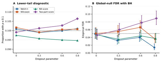
The pooled proportion of null p-values below 0.1 stays close to 0.1 for the Welch, Wilcoxon, and two-part statistics, while the NB score is mildly conservative by this coarse measure (Figure 1). Tail behavior after BH is less uniform. Welch–BH empirical FDR drops from 0.049 at to 0.014 at ; NB–BH ranges from 0.035 to 0.047. Wilcoxon–BH reaches 0.066 at , with a Wilson interval of . The two-part score reaches 0.078 and 0.089 at and , with lower interval bounds above 0.05. These estimates show no common upward FDR trend with dropout. The independent validation below assesses whether the high-dropout excess recurs.
Figure 1.
Base ZINB global-null calibration over 1000 replicates. (A) Fraction of pooled null p-values below 0.1. (B) Empirical FDR for BH with pointwise Wilson 95% intervals. Dashed lines denote the nominal values 0.1 and 0.05.
The full null simulation also permits a BH-scale tail check (Supplementary Section S7). At , the fraction of Wilcoxon null p-values below is 0.000310, while the two-part fraction is 0.000375. The two-part fraction rises to 0.000465 at . Each fraction pools 200,000 gene scores, with Monte Carlo variability across the 1000 datasets; these are tail diagnostics rather than separate FDR estimates. For the two-part score, is at and 0.0103 at , while is 1.012 and 1.037. Thus, the covariance is small in these settings, but the unit-variance normal reference is imperfect.
The permutation check offers a second diagnostic. At , 0.0101 of two-part normal-reference p-values are at most 0.01, compared with 0.0076 of their permutation-calibrated counterparts; their paired difference is 0.0025 with Monte Carlo standard error 0.00082 across 40 datasets. The corresponding Wilcoxon fractions are 0.0088 and 0.0084. Among the permuted two-part scores, the fraction whose normal-reference p-value is below 0.00025 is 0.000345 at and 0.000527 at , compared with the nominal 0.00025. Thus, a reference-distribution mismatch contributes to the two-part extreme-tail excess in these settings. The analogous Wilcoxon permutation fractions are 0.000225 and 0.000200, so this limited check does not explain its observed 0.066 global-null FDR at .
In the independent validation, Wilcoxon–BH FDR is 0.0432 at and 0.0368 at (Supplementary Table S15). The original 0.066 estimate is therefore not reproduced in this larger run and should not be taken as evidence of persistent Wilcoxon inflation. By contrast, two-part-score–BH FDR is 0.0642 and 0.1036 , respectively. Its extreme-tail excess also persists. Table 2 reports the primary experiment, and Supplementary Table S15 reports the independent validation.
Table 2.
Empirical global-null FDR for BH with pointwise Wilson 95% intervals in brackets. Each entry is based on 1000 replicates.
4.2. Null-Score Variance and e-BH
The stress test agrees with Equation (9). At , the theoretical mean working e-value is 1.228 and the Monte Carlo mean is 1.222, yet e-BH makes no rejection in 2000 replicates. At , the theoretical mean is 61.868 and the empirical global-null FDR is 0.312, with a Wilson interval of (Supplementary Figure S1). Exceeding the null expectation bound does not necessarily lead to observed rejections in a finite simulation. This shows why empirical conservatism in a particular simulation cannot replace the verification of the e-value condition.
The ZINB null-score audit gives mean working evidence of 1.057 for the two-part score at and 1.276 at for (Supplementary Section S7). These finite Monte Carlo estimates do not certify the exact expectation. The sensitivity check also shows that c affects power: at , Welch–e-BH power is 0.001, 0.575, and 0.762 for , respectively. The higher power at does not establish validity. The null e-value condition must still be assessed for that transformation.
4.3. Mean Shifts: FDR and Power Across Dropout Levels
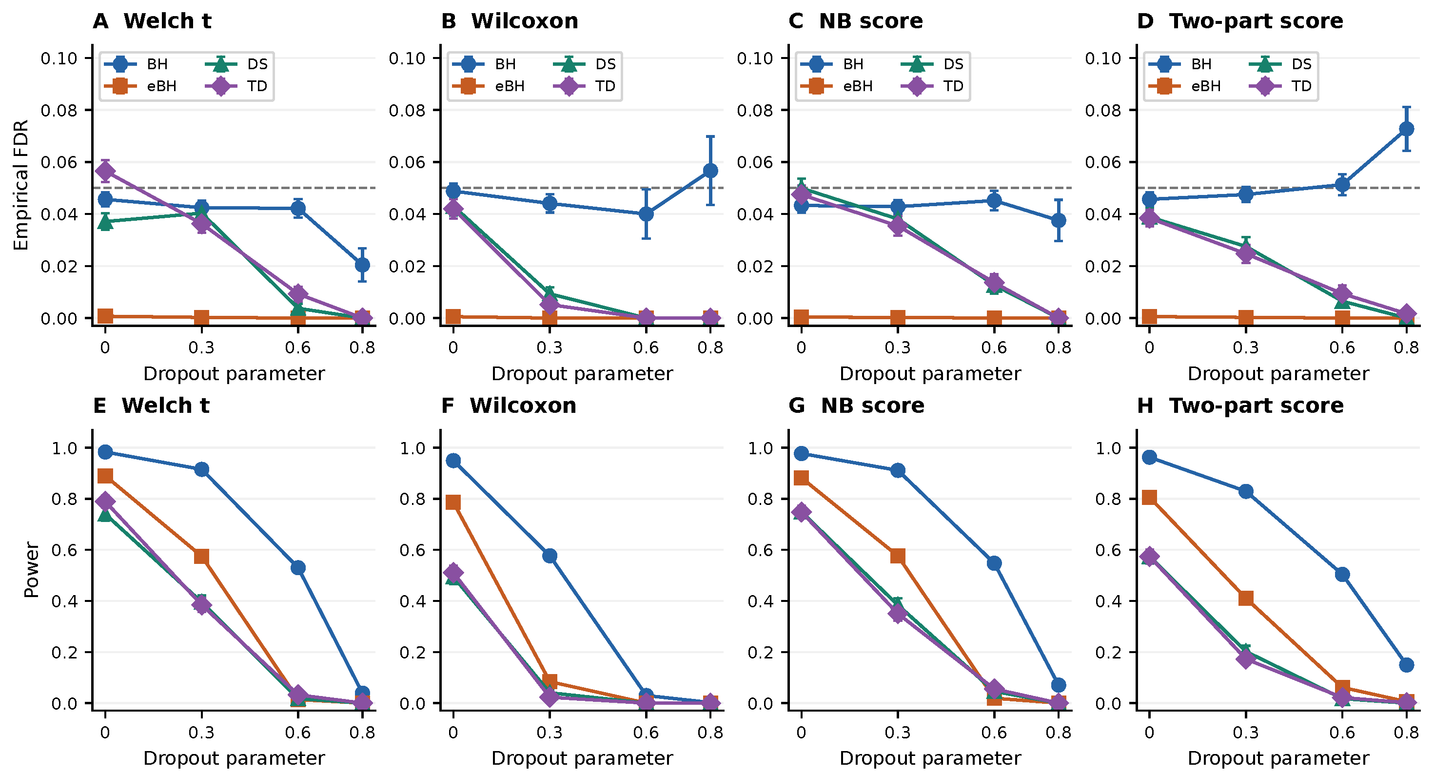
At , Welch–BH has an empirical FDR of 0.042 and a power of 0.915 in the 300-replicate base experiment. Welch–DS and Welch–TD are more conservative, with empirical FDR 0.040 and 0.036, but their powers are 0.395 and 0.384. The loss comes partly from halving the data for DS and partly from the plus-one threshold shared by DS and TD. With only 20 signals, these procedures operate near their minimum number of positive scores.
Power is non-increasing across dropout settings for all 16 statistic–rule combinations in the 300-replicate mean-shift experiment (Figure 2). For Wilcoxon paired with e-BH, DS, or TD, power is zero at both and ; the other 13 combinations decrease at each successive setting. This pattern is clearer than any common FDR trend. e-BH makes few or no discoveries in several high-dropout settings because the fixed normal-mixture evidence rarely reaches the e-BH threshold. These observations concern the chosen construction and do not imply that every valid e-value construction is uninformative.
Figure 2.
Mean-shift results in the base ZINB experiment over 300 replicates. (A) Empirical FDR for the Welch t-statistic; (B) empirical FDR for the Wilcoxon statistic; (C) empirical FDR for the NB score; (D) empirical FDR for the two-part score; (E) power for the Welch t-statistic; (F) power for the Wilcoxon statistic; (G) power for the NB score; (H) power for the two-part score. Each panel compares BH, e-BH, DS, and TD across dropout levels. Error bars represent one Monte Carlo standard error. Dashed lines in panels (A–D) mark the nominal FDR level of 0.05.
4.4. FDR and Power at Different Gene and Signal Counts
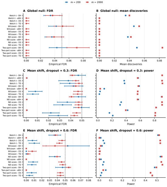
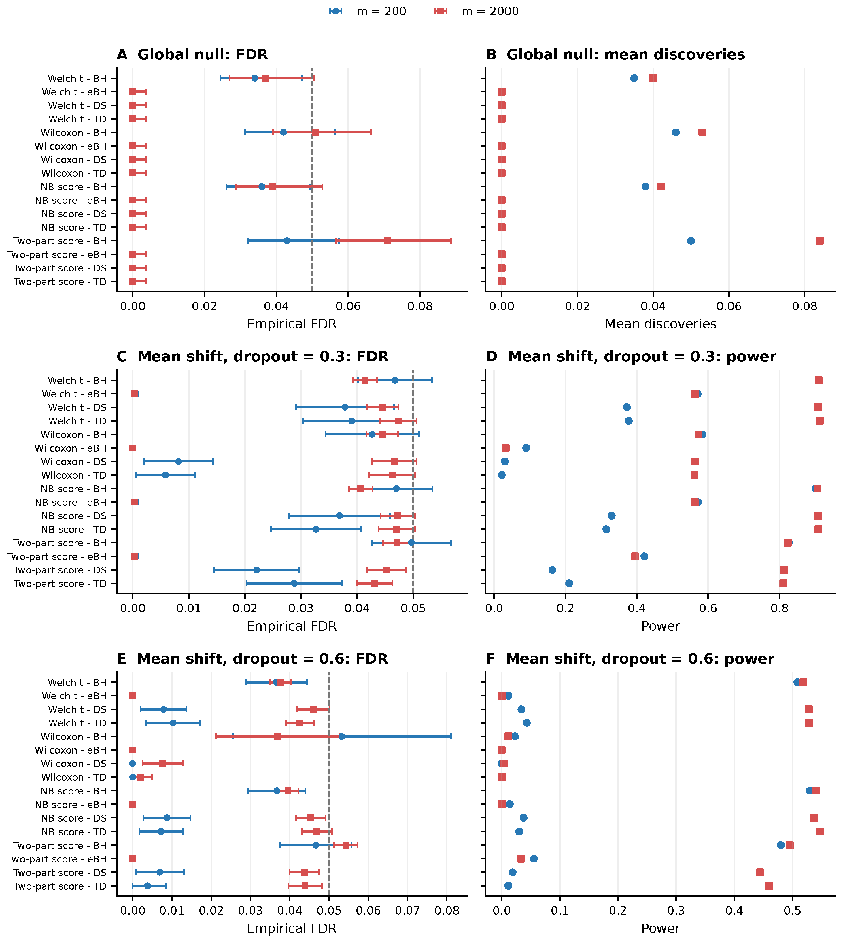
The experiment places DS and TD near their minimum positive-score requirement. At , Welch–DS and Welch–TD have powers of 0.373 and 0.378 with 200 genes. With 2000 genes and the same 10% signal proportion, the corresponding powers rise to 0.909 and 0.913 (Figure 3). This fixed-proportion comparison changes the number of true signals from 20 to 200 as well as the testing burden. The two-part DS and TD powers similarly rise from 0.164 and 0.210 to 0.813 and 0.811.
Figure 3.
Gene-scale comparison with a fixed non-null proportion in the mean-shift settings. (A) Global-null empirical FDR; (B) global-null mean discoveries; (C) mean-shift empirical FDR at ; (D) mean-shift power at ; (E) mean-shift empirical FDR at ; (F) mean-shift power at . Blue circles represent , and red squares represent . The non-null proportion is 0.1 in the mean-shift settings; all genes are null in the global-null settings. The fixed-signal comparison is reported separately in the Supplementary Materials. Global-null summaries use 1000 replicates, and mean-shift summaries use 200 replicates. Horizontal error bars in panels (A,C,E) show pointwise 95% intervals; dashed lines mark the nominal FDR level of 0.05.
The fixed-signal comparison separates these changes (Supplementary Section S7). With but only 20 signals at , Welch–DS and Welch–TD power is 0.135 and 0.131, with pointwise 95% Monte Carlo intervals of and . Welch–BH power also falls from 0.910 at to 0.771 at . Thus, increasing m while keeping fixed does not reproduce the fixed-proportion DS/TD power gain; the gain in the fixed-proportion comparison depends substantially on having more signals. The same qualitative contrast appears at .
The larger gene universe also makes tail calibration more visible. Under the global null, two-part-score–BH has empirical FDR 0.071 with a Wilson interval of . For all four statistics, DS, TD, and e-BH make no discoveries in the 1000 recorded null replicates, so their empirical FDR and mean discoveries are both zero. Under the global null, FDR equals ; a zero estimate here mainly describes no observed rejections, with Wilson upper bound 0.0038, and does not establish validity or power. The 200-gene setting is useful for mechanism checks, while the larger setting tests a more stringent multiplicity threshold.
4.5. Detecting Dispersion Changes at Equal Means
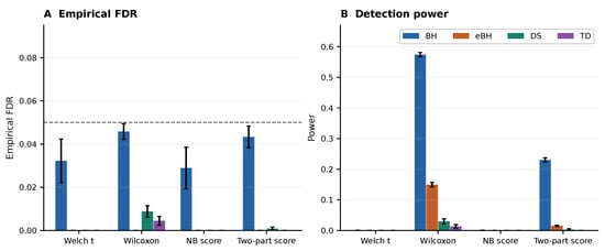
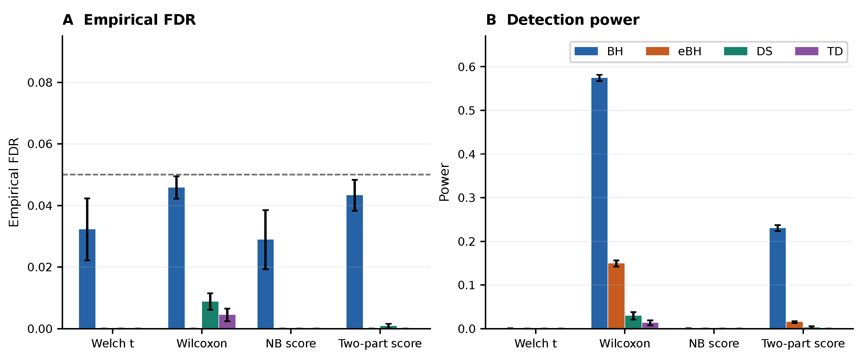
When only dispersion changes, Welch–BH and NB-score–BH both have a power of 0.0005. In contrast, Wilcoxon–BH reaches a power of 0.574 and two-part-score–BH reaches 0.230 (Figure 4). Their empirical FDR values are 0.046 and 0.043. The Wilcoxon statistic responds to distributional rank changes, while the two-part statistic responds to the altered zero probability and positive-count distribution. These results do not show that one statistic is uniformly better; they show that a mean test and a distribution-sensitive test answer different questions.
Figure 4.
Equal-mean dispersion-change results at over 300 replicates. (A) Empirical FDR, calculated as the mean replicate FDP; (B) detection power, calculated as the mean replicate true-positive proportion. Both panels compare the four statistics paired with BH, e-BH, DS, and TD. Blue, orange, green, and purple bars represent BH, e-BH, DS, and TD, respectively, in both panels. Black error bars represent one Monte Carlo standard error. The dashed line in panel (A) marks the nominal FDR level of 0.05.
4.6. Effects of Donor Number and Gene Dependence
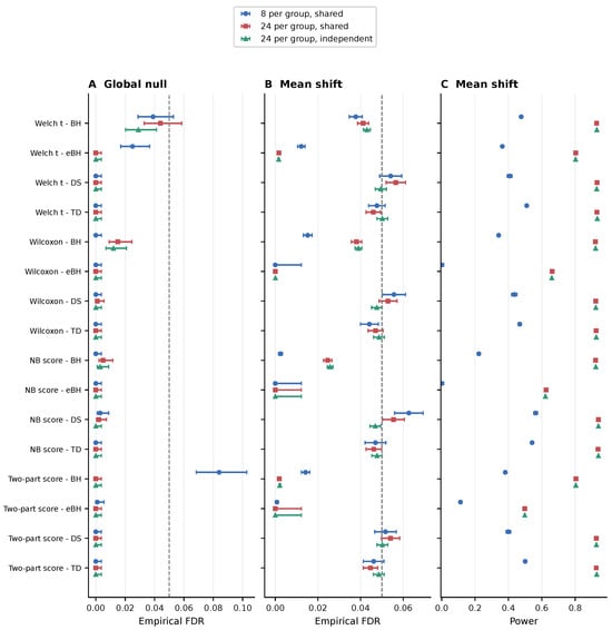
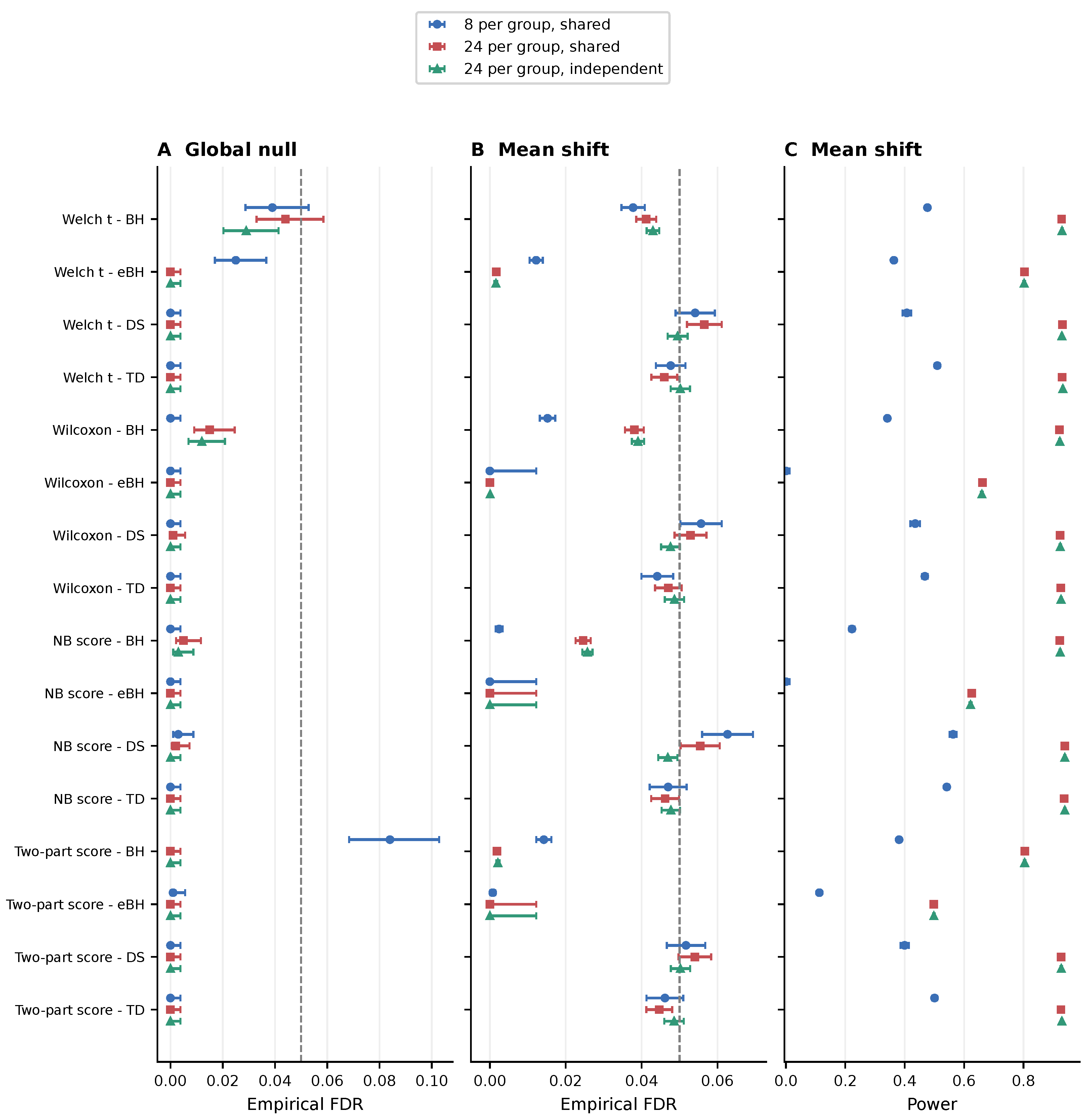
The Kang18-derived experiment directly evaluates the same 16 statistic–rule combinations as the ZINB benchmark (Figure 5). Under the shared-template global null with 8 donors per group, two-part-score–BH has empirical FDR 0.084 with a Wilson interval of . This result is consistent with the extreme-tail diagnostic: Although only 0.0145 of its null p-values are below 0.05, approximately are below , compared with the nominal . A coarse central-tail diagnostic can therefore look conservative while the BH-relevant extreme tail is anti-conservative.
Figure 5.
Performance in the Kang18-derived known-truth experiment. The three configurations use 8 donors per group with shared templates, 24 donors with shared templates, and 24 donors with gene-independent templates. (A) Global-null FDR. (B) Mean-shift FDR. (C) Mean-shift power. Intervals are pointwise 95% intervals.
With 24 donors and a mean shift, Welch–DS has an average FDP of 0.0565 under shared templates and 0.0495 under gene-independent templates. The respective Monte Carlo standard errors are 0.00234 and 0.00134. Their difference is 0.0070, with an approximate independent-run Monte Carlo interval of . Because the marginal single-gene distributions are identical between these two modes, this contrast is consistent with an effect of the changed joint structure in this fitted model. It is not a general theorem about dependent genes.
Sample size has a larger effect on power. Welch–BH power rises from 0.477 with 8 shared-template donors to 0.928 with 24. Welch–TD rises from 0.510 to 0.930. With 24 shared-template donors, all four TD combinations have an average FDP between 0.0447 and 0.0471 and a power between 0.925 and 0.937. With only 8 donors, however, NB-score–DS has an average FDP of 0.0627 and a power of 0.563. No statistic–rule pair dominates across donor counts and evidence conditions.
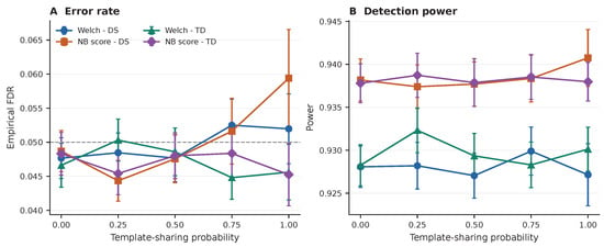
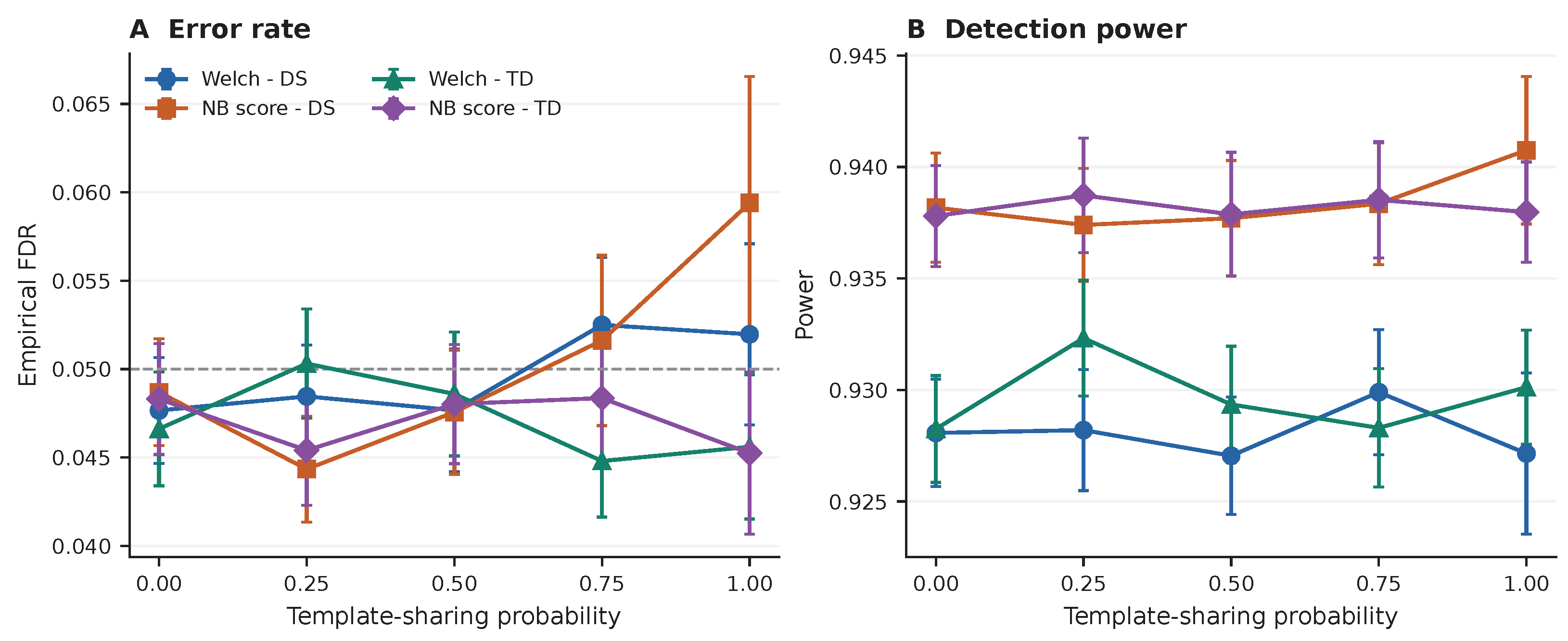
The dependence gradient gives a more detailed view than the two endpoint modes (Figure 6). NB-score–DS has empirical FDR 0.0487, 0.0443, 0.0476, 0.0516, and 0.0594 as increases from 0 to 1. Welch–DS has corresponding values 0.0477, 0.0485, 0.0477, 0.0525, and 0.0520. The changes are not monotone, but some DS estimates are higher at the most strongly shared settings. The displayed TD estimates remain near 0.045–0.050. Power changes little across for these four combinations because the marginal gene distributions and effect sizes are fixed. In the fitted null generator, median absolute pairwise gene correlation rises from zero at to 0.036 at ; its 90th percentile reaches 0.153 (Supplementary Section S7). These values quantify the dependence generated by the chosen templates, not dependence in all single-cell datasets.
Figure 6.
Dependence-gradient results with 24 donors per group, 2000 genes, and 200 Monte Carlo replicates per setting. (A) Empirical FDR; (B) detection power. Both panels compare the Welch t-statistic and NB score paired with DS and TD. The template-sharing probability ranges from gene-independent templates () to a shared donor template (). Error bars show pointwise 95% Monte Carlo intervals. The dashed line in panel (A) marks the nominal FDR level of 0.05.
5. Discussion
The benchmark does not support a single ranking of FDR procedures. In the base simulation, dropout mostly reduces power, while global-null FDR changes in different directions across statistics. The two-part score detects part of the dispersion alternative but has anti-conservative extreme-tail behavior in several sparse null settings. This excess persists in the independent validation, whereas the initial Wilcoxon–BH excess does not. Signal sensitivity and null calibration therefore need separate evaluation.
The working e-value experiment distinguishes empirical FDR from validity of the input evidence. Equation (9) shows that a centered normal score with variance only slightly above one already violates the null first-moment condition. The simulation at produced no rejections even though the expected evidence exceeded one. An apparently conservative empirical FDR can therefore coexist with invalid input evidence. The e-BH results in this paper describe the fixed construction and should not be generalized to other valid e-value constructions.
The gene-scale experiment changes the practical comparison of DS and TD. A 200-gene benchmark with 20 signals places both procedures near the discrete boundary imposed by the plus-one numerator. The fixed-proportion comparison gives them more signals when the tested universe grows; the fixed-signal comparison shows lower power with 2000 tests. Both the number of tests and the number of signals therefore matter. The 2000-gene null setting also probes smaller p-value thresholds and reveals calibration problems that a smaller experiment can miss.
A descriptive decomposition summarizes variation across the 64 mean-shift grid cells (Supplementary Figure S4). Across the selected cell means, the FDR-procedure factor accounts for 56.0% of the sum of squares in empirical FDR, dropout for 16.2%, and their interaction for 16.5%; the statistic factor accounts for 0.8%. For power, dropout accounts for 70.8%, followed by the FDR procedure at 14.9% and the statistic at 4.2%. These are arithmetic shares across fixed simulation settings. The calculation has no sampling model for factor levels or within-cell error term, and no significance test is performed. The shares describe this grid and should not be interpreted as population or causal effects.
The Kang18-derived analysis uses observed control donors only to build an empirical reference distribution. Simulated labels and signal genes provide known truth for comparing procedures. The dependence gradient shows that increasing template sharing does not create a common monotone FDR response, although DS estimates tend to be higher at the strongest sharing levels. Because each gene has the same marginal distribution across , the observed changes arise from the joint structure and Monte Carlo variation rather than from a change in the single-gene model.
The donor-derived design remains conditional on eight fitted control donors. It uses a common library scale, does not reconstruct cell-level zeros, and does not reproduce the paired interferon response. Its shared-template mechanism is simpler than a full biological latent-factor model. Pseudobulk and mixed-model analyses remain appropriate when observed biological replicates define the sampling unit [25,26]. The separate paired-donor software check in Supplementary Table S7 gives, at , global-null FDR estimates of 0.150 for DESeq2 and 0.040 for MAST over 100 replicates, and mean-shift powers of 0.847 and 0.713 over 30 replicates. These configuration-specific values are reported to distinguish the official workflows from our simplified scores, not to rank the two packages.
Other limits concern the procedures themselves. A single split is used for DS, while repeated or aggregated splitting could reduce variability. The plus-one DS rule is one mirror implementation rather than a reproduction of all variants in the original framework. TD uses one gene-wise permutation, and a general guarantee would require stronger joint exchangeability conditions than marginal target–decoy similarity. The study also does not compare adaptive methods based on an estimated null proportion or informative covariates [27,28]. Across the settings studied here, signal type changes which statistics detect alternatives, high-dropout null tails affect some BH results, and the balance between tested genes and true signals affects DS/TD power. The donor-template results are conditional on one fitted dependence model.
6. Conclusions
Single-cell DE performance depends jointly on the gene-level statistic and the FDR procedure. In these experiments, the statistic affects sensitivity to the simulated alternative and null-tail calibration. The number of tested genes and the number of signals jointly affect DS/TD power. The fitted donor dependence changes some FDR estimates without changing marginal gene distributions. The working e-value calculation shows why its null expectation must be checked before interpreting e-BH results. These conclusions are conditional on the simulated signal and dependence models and on the particular working evidence used here.
Supplementary Materials
The following supporting information can be downloaded at https://www.mdpi.com/article/10.3390/math14203786/s1, Supporting information includes implementation details, the working e-value sensitivity experiment, full numerical tables, donor-model and null-tail diagnostics, a fixed-signal gene-scale comparison, permutation calibration checks, independent null validation, the descriptive factor decomposition, the paired-donor software check, and code and seed documentation.
Author Contributions
Conceptualization, B.D. and P.H.; methodology, B.D. and Q.Z.; software, B.D.; formal analysis, B.D. and Q.Z.; writing—original draft preparation, B.D.; writing—review and editing, Q.Z. and P.H.; supervision, P.H. All authors have read and agreed to the published version of the manuscript.
Funding
This research is part of a joint doctoral program between Yunnan University and the Chinese Academy of Sciences, funded by the Academy of Mathematics and Systems Science, Chinese Academy of Sciences. It was also supported by the National Key R&D Program of China (Project No. 2022YFA1003701).
Institutional Review Board Statement
This study uses simulated data and secondary analysis of a publicly available, de-identified single-cell dataset; no new participant recruitment or intervention was performed.
Data Availability Statement
The simulation datasets were generated according to the models and settings described in this article; the numerical summaries supporting the findings are reported in the article and Supplementary Materials. The publicly available Kang18 single-cell data used to fit the donor reference model can be obtained from GEO under accession GSE96583 [17]. Method implementations are available at https://github.com/bwduan2021/single-cell-fdr-benchmark (accessed on 14 October 2026); data provenance, software versions, and random-seed specifications are provided in Supplementary Section S8.
Acknowledgments
The authors used Codex (GPT-5.6 Sol) (OpenAI; accessed September–October 2026) for English-language editing, manuscript restructuring, and debugging and standardization of selected code. The authors reviewed the outputs and take responsibility for the article.
Conflicts of Interest
The authors declare no conflicts of interest.
Abbreviations
The following abbreviations are used in this manuscript:
| BH | Benjamini–Hochberg |
| DS | data splitting |
| FDP | false discovery proportion |
| FDR | false discovery rate |
| MCSE | Monte Carlo standard error |
| NB | negative binomial |
| TD | target–decoy competition |
| ZINB | zero-inflated negative binomial |
References
- Zheng, G.X.Y.; Terry, J.M.; Belgrader, P.; Ryvkin, P.; Bent, Z.W.; Wilson, R.; Ziraldo, S.B.; Wheeler, T.D.; McDermott, G.P.; Zhu, J.; et al. Massively parallel digital transcriptional profiling of single cells. Nat. Commun. 2017, 8, 14049. [Google Scholar] [CrossRef] [Scilit]
- Kharchenko, P.V.; Silberstein, L.; Scadden, D.T. Bayesian approach to single-cell differential expression analysis. Nat. Methods 2014, 11, 740–742. [Google Scholar] [CrossRef] [Scilit]
- Lun, A.T.L.; Bach, K.; Marioni, J.C. Pooling across cells to normalize single-cell RNA sequencing data with many zero counts. Genome Biol. 2016, 17, 75. [Google Scholar] [CrossRef] [Scilit]
- Svensson, V. Droplet scRNA-seq is not zero-inflated. Nat. Biotechnol. 2020, 38, 147–150. [Google Scholar] [CrossRef] [Scilit]
- Jaakkola, M.K.; Seyednasrollah, F.; Mehmood, A.; Elo, L.L. Comparison of methods to detect differentially expressed genes between single-cell populations. Brief. Bioinform. 2017, 18, 735–743. [Google Scholar] [CrossRef] [Scilit]
- Soneson, C.; Robinson, M.D. Bias, robustness and scalability in single-cell differential expression analysis. Nat. Methods 2018, 15, 255–261. [Google Scholar] [CrossRef] [Scilit]
- Squair, J.W.; Gautier, M.; Kathe, C.; Anderson, M.A.; James, N.D.; Hutson, T.H.; Hudelle, R.; Qaiser, T.; Matson, K.J.E.; Barraud, Q.; et al. Confronting false discoveries in single-cell differential expression. Nat. Commun. 2021, 12, 5692. [Google Scholar] [CrossRef] [Scilit]
- Korthauer, K.D.; Chu, L.F.; Newton, M.A.; Li, Y.; Thomson, J.; Stewart, R.; Kendziorski, C. A statistical approach for identifying differential distributions in single-cell RNA-seq experiments. Genome Biol. 2016, 17, 222. [Google Scholar] [CrossRef] [Scilit]
- Delmans, M.; Hemberg, M. Discrete distributional differential expression (D3E)—A tool for gene expression analysis of single-cell RNA-seq data. BMC Bioinform. 2016, 17, 110. [Google Scholar] [CrossRef] [Scilit]
- Benjamini, Y.; Hochberg, Y. Controlling the false discovery rate: A practical and powerful approach to multiple testing. J. R. Stat. Soc. Ser. B 1995, 57, 289–300. [Google Scholar] [CrossRef] [Scilit]
- Benjamini, Y.; Yekutieli, D. The control of the false discovery rate in multiple testing under dependency. Ann. Stat. 2001, 29, 1165–1188. [Google Scholar] [CrossRef] [Scilit]
- Wang, R.; Ramdas, A. False discovery rate control with e-values. J. R. Stat. Soc. Ser. B 2022, 84, 822–852. [Google Scholar] [CrossRef] [Scilit]
- Dai, C.; Lin, B.; Xing, X.; Liu, J.S. False discovery rate control via data splitting. J. Am. Stat. Assoc. 2023, 118, 2503–2520. [Google Scholar] [CrossRef] [Scilit]
- Elias, J.E.; Gygi, S.P. Target-decoy search strategy for increased confidence in large-scale protein identifications by mass spectrometry. Nat. Methods 2007, 4, 207–214. [Google Scholar] [CrossRef] [Scilit]
- He, K.; Li, M.J.; Fu, Y.; Gong, F.Z.; Sun, X.M. Null-free false discovery rate control using decoy permutations. Acta Math. Appl. Sin. Engl. Ser. 2022, 38, 235–253. [Google Scholar] [CrossRef] [Scilit]
- Ge, X.; Chen, Y.E.; Song, D.; McDermott, M.; Woyshner, K.; Manousopoulou, A.; Wang, N.; Li, W.; Wang, L.D.; Li, J.J. Clipper: p-value-free FDR control on high-throughput data from two conditions. Genome Biol. 2021, 22, 288. [Google Scholar] [CrossRef] [Scilit]
- Kang, H.M.; Subramaniam, M.; Targ, S.; Nguyen, M.; Maliskova, L.; McCarthy, E.; Wan, E.; Wong, S.; Byrnes, L.; Lanata, C.M.; et al. Multiplexed droplet single-cell RNA-sequencing using natural genetic variation. Nat. Biotechnol. 2018, 36, 89–94. [Google Scholar] [CrossRef] [Scilit]
- Love, M.I.; Huber, W.; Anders, S. Moderated estimation of fold change and dispersion for RNA-seq data with DESeq2. Genome Biol. 2014, 15, 550. [Google Scholar] [CrossRef] [Scilit]
- Finak, G.; McDavid, A.; Yajima, M.; Deng, J.; Gersuk, V.; Shalek, A.K.; Slichter, C.K.; Miller, H.W.; McElrath, M.J.; Prlic, M.; et al. MAST: A flexible statistical framework for assessing transcriptional changes and characterizing heterogeneity in single-cell RNA sequencing data. Genome Biol. 2015, 16, 278. [Google Scholar] [CrossRef] [Scilit]
- Welch, B.L. The generalization of “Student’s” problem when several different population variances are involved. Biometrika 1947, 34, 28–35. [Google Scholar] [CrossRef] [Scilit]
- Wilcoxon, F. Individual comparisons by ranking methods. Biom. Bull. 1945, 1, 80–83. [Google Scholar] [CrossRef] [Scilit]
- Mann, H.B.; Whitney, D.R. On a test of whether one of two random variables is stochastically larger than the other. Ann. Math. Stat. 1947, 18, 50–60. [Google Scholar] [CrossRef] [Scilit]
- Robinson, M.D.; Smyth, G.K. Small-sample estimation of negative binomial dispersion, with applications to SAGE data. Biostatistics 2008, 9, 321–332. [Google Scholar] [CrossRef] [Scilit]
- Zappia, L.; Phipson, B.; Oshlack, A. Splatter: Simulation of single-cell RNA sequencing data. Genome Biol. 2017, 18, 174. [Google Scholar] [CrossRef] [Scilit]
- Crowell, H.L.; Soneson, C.; Germain, P.L.; Calini, D.; Collin, L.; Raposo, C.; Malhotra, D.; Robinson, M.D. muscat detects subpopulation-specific state transitions from multi-sample multi-condition single-cell transcriptomics data. Nat. Commun. 2020, 11, 6077. [Google Scholar] [CrossRef] [Scilit]
- Zimmerman, K.D.; Espeland, M.A.; Langefeld, C.D. A practical solution to pseudoreplication bias in single-cell studies. Nat. Commun. 2021, 12, 738. [Google Scholar] [CrossRef] [Scilit]
- Storey, J.D. A direct approach to false discovery rates. J. R. Stat. Soc. Ser. B 2002, 64, 479–498. [Google Scholar] [CrossRef] [Scilit]
- Ignatiadis, N.; Klaus, B.; Zaugg, J.B.; Huber, W. Data-driven hypothesis weighting increases detection power in genome-scale multiple testing. Nat. Methods 2016, 13, 577–580. [Google Scholar] [CrossRef] [Scilit]

Disclaimer/Publisher’s Note: The statements, opinions and data contained in all publications are solely those of the individual author(s) and contributor(s) and not of MDPI and/or the editor(s). MDPI and/or the editor(s) disclaim responsibility for any injury to people or property resulting from any ideas, methods, instructions or products referred to in the content. |
© 2026 by the authors. Licensee MDPI, Basel, Switzerland. This article is an open access article distributed under the terms and conditions of the Creative Commons Attribution (CC BY) license.