


Abstract
Conjunction assessment needs risk screening that is early, scalable and interpretable. We ask whether projected quantum feature maps add predictive value to this task when compared with strong classical learners under strict leakage control. From 149,044 real SOCRATES conjunction events (119,568 object pairs), split pair-disjointly, we predict the base-ten logarithm of the maximum collision probability. We prove that the pair-disjoint held-out loss is unbiased for the risk on unseen pairs, that the logarithmic target preserves risk ranking, that the local six-qubit feature map is exactly a classical additive model, and when a validation-fitted ensemble assigns a member zero weight. In the configuration fixed a priori (encoding bandwidth , linear outer kernel), the projected models trail gradient boosting ( and against ), and the local map is no better than a linear ridge on the raw inputs. Matched experiments on identical training sets show that this shortfall comes from two design choices rather than from the representation: the bandwidth folds the dominant descriptors, and the linear outer kernel discards nonlinear structure. With a validated bandwidth and a Gaussian outer kernel, the local projected model outperforms a tuned classical Gaussian kernel on 1200-event subsets in all five draws () and has the lowest point estimate at full scale (), where it is statistically tied with that kernel. It takes the largest weight in an ensemble that lowers from to . This is not a quantum advantage: the local model is classically computable in closed form, and the interaction pattern of the entangled variant never improves accuracy. In 200 randomly seeded configurations at and , it reduces it, and at the validated bandwidth the difference is not significant at full scale.
Keywords:
quantum machine learning; projected quantum kernels; conjunction assessment; space situational awareness; satellite collision risk; SOCRATES; kernel methods; ridge regression; ensemble learning; leakage control MSC:
81P68; 68T05; 62J07; 70M20
1. Introduction
Space near the Earth used to be a fairly quiet place for a small number of large spacecraft. That is no longer true. Large constellations, active payloads, spent rocket bodies, and countless fragments now share the same shells of low Earth orbit [1]. The practical result is simple to state and hard to handle: the number of possible close approaches grows faster than any human team can review by hand. Modern space traffic coordination therefore leans on automated screening, risk ranking, and tools that turn a huge catalogue into a short list of cases that a person actually needs to look at [2,3].
Conjunction assessment (CA) sits at the centre of this process. A typical CA pipeline starts from object states, propagates the orbits, finds close approaches, estimates miss distance and relative velocity, and finally assigns a probability-related risk number. Operational systems often report a maximum collision probability rather than a single miss distance, because one distance value cannot capture the uncertainty in the encounter [4]. CelesTrak’s SOCRATES service is a useful public example. It screens active payloads against the public catalogue using SGP4 propagation and reports the time of closest approach, minimum range, relative speed, maximum probability, and a dilution threshold [5,6]. These properties make SOCRATES a convenient testbed for method development, and they also make leakage control essential, because some reported fields are mathematically tied to the target.
The scale of the problem drives the need for speed and reliability at the same time. Recent work has explored deep learning for all-vs-all screening, machine learning for orbit prediction, and data-driven collision-risk estimation [2,3,7,8,9]. However, operational studies keep returning to the same warnings. Data scarcity, uncertainty growth, and the demand for explainability remain real barriers to fully automated, AI-based risk assessment.
Quantum machine learning (QML) offers a different angle. Instead of replacing the orbital-mechanics pipeline with a large network, a quantum feature map can turn a short, physically meaningful descriptor vector into a nonlinear representation, and a classical kernel learner can then use that representation. This route is attractive for engineering problems because the circuit is small, explicit, and open to mathematical study [10,11]. However, the QML literature is now very clear that quantum kernels do not beat strong classical models by default. Projected quantum kernels were proposed partly to dodge the concentration behaviour of global fidelity kernels in exponentially large Hilbert spaces [12]. Later analyses showed that this concentration can be severe and that performance depends heavily on the data encoding, the circuit design, and the kernel normalisation [13,14,15]. Large benchmarking efforts warn against reading a quantum advantage off a small gain or a favourable training loss [16,17,18].
This paper therefore asks a narrow but important question: can a projected quantum-kernel representation carry useful information for real satellite conjunction-risk prediction, once it is measured against strong classical learners under strict leakage controls?
The central object of study is the vector of encounter descriptors:
where and are the days-since-epoch descriptors of the two objects, is their difference, is the relative speed, is the minimum range at the time of closest approach, is the dilution threshold, the uncertainty descriptor, and collects the calendar timing terms. The learning target is the transformed maximum probability
which compresses a very wide dynamic range while keeping the ordering of risk scores intact.
1.1. Problem Statement
There is little evidence about how projected quantum kernels behave on real, operational conjunction data under a protocol that blocks pair-level and temporal leakage. Most quantum-kernel studies use generic benchmark datasets, and most space-AI studies use only classical models. A fair comparison needs careful data splitting, target-leakage control, uncertainty-aware evaluation, calibration, and a test of generalisation over time. A careless random split can make a quantum model look strong simply because the same object pair, or a near-identical temporal pattern, appears in both training and test.
1.2. Contributions
We make five contributions:
- A leakage-controlled, real-data benchmark with two primary settings: We build a clean benchmark from 149,044 real SOCRATES events and 119,568 unique object pairs, with a strict pair-disjoint split and a separate chronological hold-out. We separate two distinct leakage channels—split leakage and target-proxy leakage—and evaluate two primary configurations—a full-feature setting and a dilution-free setting—so that the reader can see which conclusions survive removal of the most likely label proxy.
- Formal estimator guarantees: We prove that pair-disjoint splitting makes the held-out loss an unbiased estimator of the risk over unseen object pairs under a grouped-exchangeability assumption (Proposition 1), and that the logarithmic target preserves risk ranking while turning multiplicative probability error into level-independent additive error (Proposition 2). These tie the two central design choices to provable properties rather than convention. We further show that the local feature map is exactly a classical additive model (Proposition 3) and characterise exactly when a validation-fitted ensemble assigns a member zero weight (Proposition 4).
- A competition-fair evaluation protocol: A validation-only non-negative ensemble lets the quantum and classical models compete on equal terms. Thresholds and weights are chosen on validation data only, and the test set is evaluated once, frozen.
- A diagnostic framework that separates geometry from accuracy: We report kernel–target alignment alongside predictive error, and we add dilution ablation, quantum training-size scaling, temporal generalisation, noise robustness, bootstrap confidence intervals, calibration, and computational cost. Matched comparisons on identical training sets at two budgets, raw-input and tuned-kernel classical controls, an encoding-bandwidth analysis, and a sweep over 200 circuit configurations then locate the source of each difference between the projected and classical models.
- An attribution of the original shortfall, and a design principle: The shortfall of the projected models in the configuration fixed a priori is traced to the encoding bandwidth and the linear outer kernel; once both are corrected, the local projected model matches a tuned classical Gaussian kernel at full scale and outperforms it on 1200-event subsets, but it is classically computable and entanglement adds nothing. From the diagnostics, we distil a concrete, physics-structured embedding principle: a future feature map should encode normalised pairwise physical interactions and covariance geometry rather than a generic nearest-neighbour ring. We state this as a testable methodological direction, not as a result that we have already validated.
1.3. Research Questions
This work is guided by six questions:
- RQ1
- Does a projected quantum-kernel representation predict competitively with strong classical tabular learners on real SOCRATES data?
- RQ2
- Does adding a fixed nearest-neighbour interaction pattern improve the learned representation relative to the local six-qubit map, which by Proposition 3 is exactly a classical additive model?
- RQ3
- Does the quantum component add complementary information to a classical ensemble?
- RQ4
- How strongly does the dilution threshold affect performance, and does this effect differ between classical and quantum representations?
- RQ5
- How does quantum performance change as the number of quantum training events grows?
- RQ6
- How robust is the quantum representation to temporal shift and input perturbation?
1.4. Paper Structure
Section 2 reviews conjunction assessment, machine learning for space situational awareness, and quantum-kernel methods. Section 3 states the prediction problem and the leakage controls. Section 4 gives the full QKODE-CE methodology, including the circuit, the projected kernel, and the ridge model, with the mathematics written to match the released code. Section 5 describes the data and the evaluation protocol. Section 6 presents the results. Section 7 discusses what they mean. Section 8 lists the limitations, and Section 9 concludes the paper. Appendix A, Appendix B and Appendix C present the algorithm, extended derivations, and full tables.
2. Related Work
2.1. Conjunction Assessment and Operational Space Safety
Operational CA blends orbital propagation, screening filters, uncertainty modelling, and human decision support. The hard part is not just computing a distance between two trajectories—the real question is whether an uncertainty-aware encounter justifies extra observations, a manoeuvre, or continued monitoring [3,9]. This matters for machine learning, because the target is usually a derived risk quantity rather than a directly observed measurement.
CelesTrak SOCRATES is a good public benchmark because the calculation is repeatable, the fields are documented, and the service refreshes on a fixed schedule. It screens active payloads against the public catalogue, uses SGP4 propagation, and searches for encounters within a set threshold over a seven-day window [5,6]. Each record carries two object identifiers, days since epoch, the time of closest approach, minimum range, relative speed, maximum probability, and a dilution threshold. The maximum probability is a conservative construction, and the dilution threshold marks a region where the link between the reported maximum and a true probability is less direct [4]. These properties make SOCRATES valuable, but they also create a leakage risk if a model quietly uses variables that are mathematically entangled with the target. QKODE-CE handles this by treating strictly as a target and by measuring the effect of dilution on its own.
The growing population drives the need for efficient screening. Stevenson et al. benchmarked deep learning for all-vs-all screening on a dataset of 170 million object pairs, showing both the promise and the computational weight of learning-based screening at operational scale [2]. The ESA collision-avoidance challenge turned a public set of conjunction data messages into a shared machine-learning task and drew a large field of competitors [3]. Our study complements these efforts by focusing on a public, real-data risk-regression target rather than a simulated all-vs-all classification task.
2.2. Machine Learning for Space Situational Awareness
Higher-fidelity numerical propagators exist and are more accurate than SGP4, but they require force models, drag and solar-radiation-pressure coefficients, and covariance information that are not published for the bulk of the catalogue. SGP4 operates directly on the public two-line element sets and is therefore the only propagator that can be applied uniformly to the entire catalogue by any group without privileged data access. Its use in public conjunction benchmarks is a reproducibility choice rather than an accuracy claim: it fixes a common, auditable baseline [5,6]. The accuracy ceiling that this imposes is shared identically by every model that we compare, so it does not favour either the classical or the quantum branch.
Realised collisions are vanishingly rare, so a model trained on raw orbital states would have to learn encounter geometry from scratch with almost no positive examples. Pairing a compact vector of physically meaningful descriptors—such as relative range, relative speed, and uncertainty scale—with a statistical model shifts the learning burden: the physics supplies the structure, and the model only has to learn a residual mapping onto the risk scale. This lowers the effective sample complexity and is why feature-based approaches remain competitive in this domain.
A conjunction score is consumed by human analysts who must decide whether to expend propellant and disrupt a mission. If the score is not calibrated, a stated risk level does not correspond to the frequency with which such events actually occur in the model’s own terms, and analysts cannot set a consistent action threshold. Miscalibration in either direction is costly: systematic overstatement drives unnecessary manoeuvres and alert fatigue, while understatement erodes the margin that the screening layer exists to protect. This is why we report Brier score and expected calibration error alongside discrimination metrics in Section 6.
Unannounced or non-cooperative manoeuvres break the ballistic assumption on which propagation rests, and they are not labelled in public catalogues. Self-supervised sequence models are a natural fit because they can be trained on unlabelled element-set histories to predict the next state, after which a manoeuvre appears as a sustained residual between prediction and observation rather than as a pre-annotated class. This is complementary to the present work, which conditions on a screening output that already assumes ballistic propagation.
Machine learning shows up across space situational awareness for orbit prediction, association, tracking, and risk assessment. Support vector regression has been used to learn orbit-prediction errors from public data [8]. Self-supervised sequence models such as ORBERT learn representations from large amounts of unlabelled orbit data and reuse them for downstream screening tasks [7]. Open toolkits like Kessler package machine-learning models and generative simulators for conjunction data messages [9]. A recurring design lesson runs through all of this: the strongest systems combine physics-based descriptors with statistical learning rather than throwing away the physical model. QKODE-CE follows that lesson. The quantum circuit does not propagate any orbits. It receives interpretable encounter descriptors and builds a nonlinear representation from them.
2.3. Quantum Machine Learning and Kernel Methods
In a standard quantum kernel workflow, each input is encoded into a state by a data-dependent circuit, and the kernel entry is the fidelity . This is read out either by the compute–uncompute construction, in which is applied to and the probability of measuring the all-zero string is estimated from repeated shots, or by a swap test on two registers. Either way, the similarity is a sampled quantity, so each Gram entry carries shot noise of order . A projected kernel instead measures a small set of local observables once per input and computes similarity classically from those vectors, which is the construction used here, and which removes the quadratic number of circuit pairs.
A q-qubit state lives in a space of dimension , whereas the encoded input carries at most d independent directions. When , the encoded states populate a low-dimensional manifold inside a very large Hilbert space, and global fidelities between distinct inputs decay towards a common small value, so off-diagonal Gram entries become nearly indistinguishable and the kernel approaches the identity. The estimation problem then becomes ill posed, because resolving genuine similarity differences requires a shot budget that grows with the concentration scale [13]. Projecting onto few-body observables restricts the representation to a space whose dimension grows linearly rather than exponentially in q, which is precisely why projected kernels were introduced [12].
Applying a linear outer kernel to the projected vector, as in Equation (35), yields a reproducing-kernel Hilbert space of exactly the same finite dimension as the projected vector (here, eighteen). The resulting hypothesis class is the set of linear functions of the measured observables, so the model is a finite-dimensional linear model in a quantum-derived coordinate system, and its capacity is bounded by that dimension irrespective of the sample size. A Gaussian outer kernel on the same projected vector induces an infinite-dimensional RKHS and can represent arbitrary smooth functions of the observables, at the cost of an extra bandwidth parameter and a Gram matrix that must be formed or approximated. The practical consequence is that the linear variant used here cannot represent nonlinear interactions among the projected observables, even though each observable is itself a nonlinear function of the input.
Quantum kernel learning has a simple shape. A quantum feature map embeds a classical vector into a quantum state,
and a similarity is read out from either state fidelity or a projected observable representation. A classical learner such as kernel ridge regression or a support vector machine then operates on that implicit feature space [11,19,20].
Huang et al. tied the power of a quantum model to the data distribution and introduced projected quantum kernels to soften concentration effects [12]. The term covers a family of constructions that share the same first step—mapping a quantum state to a vector of projected observables—but differ in the outer kernel applied to that vector. Huang et al.’s original construction and much follow-up work use a Gaussian outer kernel on the projected vector, while QKODE-CE uses a linear outer kernel and states this choice explicitly wherever the model is described, since the two give different function classes and different concentration behaviour. Thanasilp et al. analysed exponential concentration in quantum kernels and showed that global kernels can drift toward the identity matrix as the circuit dimension grows [13]. This is directly relevant here, because our input dimension is modest while the underlying state dimension is exponential in the qubit count. The data encoding matters too. Schuld et al. showed that the encoding gates set the accessible frequency spectrum and, therefore, the expressive power of the model [21]. Pérez-Salinas et al. showed that repeated data re-uploading can make shallow circuits surprisingly expressive [22]. Jerbi et al. unified many circuit models as linear models in quantum feature space, clarifying what a projected map can and cannot buy [23]. None of these results imply that a more expressive circuit is automatically better on a fixed finite dataset.
Recent benchmarking makes that point sharply. Schnabel and Roth evaluated fidelity and projected quantum kernels across five dataset families, 64 datasets, and more than twenty thousand models, and they found strong sensitivity to encoding, kernel, and hyperparameter choices with no universal advantage [16]. Bandwidth tuning can even push a quantum kernel to behave like a classical one [15,24]. Numerical studies find little advantage from fidelity kernels on classical data [18], and careful benchmarking guides warn about common pitfalls in QML evaluation [17,25].
2.4. Research Gap
Beyond Kernel Methods: Uncertainty-Aware Quantum Machine Intelligence
Quantum machine learning is broader than the kernel paradigm evaluated here, and a negative kernel result should be read against that wider landscape. One strand that is particularly relevant to conjunction assessment couples quantum computation with evidential reasoning based on belief functions. The transferable belief model of Smets and Kennes represents graded belief at a credal level using set-valued masses over a frame of discernment, and it converts belief to a decision-ready probability only at the pignistic level when an action is required [26,27]. Unlike a single probability, this formalism separates genuine evidential support from ignorance, which matches the situation in conjunction screening, where a low computed probability may reflect either a benign geometry or an essentially unknown covariance.
The classical obstacle is cost: belief operations range over the power set and, thus, scale exponentially in the size of the frame. Recent work formulates transferable belief model reasoning directly on quantum circuits, encoding mass functions as quantum states and implementing credal-level fusion, correction, and the generalised Bayesian theorem with gate counts that grow linearly rather than exponentially in the number of frame elements [28]. Belief functions also have an established track record in aerospace tracking and target classification, including within the transferable belief model itself [29,30], which makes this a natural bridge to space situational awareness.
This direction differs from ours in an important way: A projected quantum kernel seeks a better similarity geometry for point prediction, and our results indicate that a generic entangled map does not supply one for this dataset. An evidential quantum formulation instead targets the representation of uncertainty itself, which is arguably the binding constraint in conjunction assessment given that dilution, the dominant feature in Section 6, is precisely an uncertainty descriptor. We therefore regard uncertainty-aware quantum machine intelligence as a more promising avenue than further tuning of fidelity-based kernels, and we return to it in Section 7.7.
Three gaps motivate this work: First, there is little evidence for quantum-kernel learning on real operational conjunction data. Second, quantum-kernel papers tend to use generic benchmarks, while the orbital-risk domain offers a structured physical setting where feature design can be tied to the geometry of encounters. Third, a fair QML comparison on this domain needs pair-disjoint splitting, target-leakage control, uncertainty-aware evaluation, calibration, and a temporal test, all at once. QKODE-CE closes these gaps without claiming that a six-qubit simulator can replace an operational CA system. The contribution is methodological and empirical: build a clean real-data benchmark, insert a physically motivated projected quantum kernel, and measure the incremental value of the quantum representation under several kinds of generalisation.
3. Problem Formulation
Consider a set of conjunction events
where is the observable feature vector from Equation (1), is the transformed maximum probability from Equation (2), is the unordered object-pair identifier, and is the timestamp of the closest approach.
The primary regression problem is to find
where ℓ is the squared loss for the kernel-ridge and ensemble components. The held-out metrics are mean absolute error (MAE), root-mean-square error, the coefficient of determination, and the Spearman rank correlation. The root-mean-square error is
and the coefficient of determination is
Spearman correlation is computed from the ranks of y and . It is useful because CA prioritisation often cares more about correct ordering than about a perfectly calibrated continuous score.
For high-risk screening, we define an event label from the validation distribution only. Let be the 90th percentile of the validation targets. Then,
No test label is used to set . For a prediction score , the operating threshold is chosen on validation data by maximising the score. The test set is then scored once with the frozen threshold.
The second key requirement is group independence. Let , , and be the sets of pair identifiers in each split. We require
This is stronger than an ordinary random split, because many events can belong to the same pair at different times. If one event from a pair lands in training and another lands in test, a flexible learner can quietly memorise pair-specific geometry and report an optimistic score.
For temporal evaluation, events are ordered by the time of closest approach. The chronological experiment uses the earliest 70% for training, the next 15% for validation, and the latest 15% for testing. This answers a different question from Equation (9): whether the model generalises to future time periods even when object-pair overlap is allowed by the chronology.
3.1. Two Notions of Information Leakage
Pair-disjoint splitting has a cost and a consequence. Grouping by object pair does not discard events, so the nominal training count is comparable to a random split, but it does reduce the effective sample size. Events sharing a pair are strongly correlated, so a pair contributes far less independent information than its event count suggests; the effective size is closer to the number of distinct pairs (here, 95,654) than to the number of events. Learning curves are therefore shifted relative to a random split, and the apparent accuracy of a randomly split benchmark is partly an artefact of counting correlated events as independent.
The operational consequence is concrete. A model validated under a random split can memorise geometry specific to pairs that it has already seen. When a new constellation is launched, every conjunction involving those objects is a genuinely unseen pair, so the memorised component transfers nothing, and accuracy degrades sharply at exactly the moment when screening matters most. A pair-disjoint estimate is the quantity that predicts this regime, which is why Proposition 1 is stated over unseen pairs rather than unseen events.
The evaluation controls two different leakage channels, and we keep them separate throughout this paper because they call for different remedies: The first is split leakage. It arises when the same object pair appears in more than one split, so that a flexible learner memorises pair-specific geometry rather than learning a transferable relationship. Split leakage is a property of the partition, and Equation (9) removes it by construction. The second is target-proxy leakage. It arises when an input feature is produced by the same upstream process that generates the label, so that the feature carries a compressed image of the target rather than independent physical evidence. The dilution field is the natural suspect here, because CelesTrak derives it inside the same covariance and probability computation that produces the maximum probability that we are trying to predict. Split leakage and target-proxy leakage are logically independent: a pair-disjoint split does nothing to remove a target proxy, and dropping a proxy feature does nothing to fix an overlapping split. For this reason, we treat the dilution-free configuration in Section 6.6 as a second primary setting rather than as a sensitivity check, and we report both settings side by side.
3.2. Estimator Properties
Two properties of the design admit short proofs. They are elementary, but stating them precisely is what separates a controlled benchmark from an ad hoc one, and they justify the two central design choices, namely, pair-disjoint splitting and the logarithmic target.
We first formalise why pair-disjoint splitting yields an unbiased generalisation estimate. Let be a population of object pairs with sampling distribution , and for a pair g let be the conditional law of an event associated with that pair. For a fixed predictor f, define the per-pair risk and the target generalisation risk over unseen pairs as
Proposition 1
(Unbiasedness under grouped exchangeability). Let the learned predictor be a function of the training events only, whose pair identifiers lie in . Suppose that the test pairs are drawn exchangeably from π and are disjoint from in the sense of Equation (9), and that for each test pair one event is scored. Then, the held-out mean loss
is an unbiased estimator of the generalisation risk, that is, .
Proof.
Condition on . By Equation (9), the test pairs are disjoint from the training pairs, so is independent of . For a single test event with pair ,
by the definition in Equation (10). Taking the expectation over and using the tower property,
Every summand in Equation (11) has the same conditional expectation by exchangeability, so linearity gives . □
Remark 1.
The independence step is exactly where an ordinary random split fails. If a pair contributes events to both and , then depends on pair-specific geometry shared with the test event, the conditioning above no longer factorises, and becomes optimistically biased. Proposition 1 therefore states precisely what Equation (9) buys: it restores the independence that makes the held-out loss an unbiased estimate. When several events per pair are averaged instead of one, the estimator remains unbiased, although within-pair correlation increases its variance.
Proposition 1 also makes precise why the two leakage channels of Section 3.1 differ in cause and in remedy, and why neither remedy substitutes for the other.
Remark 2
(Split leakage is an estimation bias; target-proxy leakage is not). The only step in the proof of Proposition 1 that can fail is the independence of from the test events, and that independence is a property of the partition. It does not involve the feature set at all. Two consequences follow: First, removing a feature, however strongly it is tied to the label, leaves the partition—and, hence, the dependence between and any test pair that also appears in training—unchanged. If the remaining descriptors still carry pair-specific information, as the days-since-epoch, range, and speed of a recurring pair do, the optimistic bias of Remark 1 persists. Dropping a target proxy therefore cannot remove split leakage. Second, the proposition holds for any feature map, including one that uses a target proxy: on a pair-disjoint split, the held-out loss of a model that uses dilution is an unbiased estimate of that model’s risk on unseen pairs. Target-proxy leakage is therefore not an estimation bias. The estimate is correct; what changes is the estimand, which becomes the risk of a predictor that has access to a byproduct of the label-generating computation. Whether that estimand is operationally meaningful is a question about the deployment setting, not about the split, and it is answered by comparing Setting A and Setting B (Section 6.6), not by changing the partition.
The chronological evaluation of Section 6 tests a third hypothesis, and the same argument shows that it is not a stricter version of the pair-disjoint test but a different one. Let and denote the event distributions before and after the chronological cut .
Corollary 1
(What the chronological split estimates). If is fitted on events with and scored on events with , then, conditional on , the held-out loss is an unbiased estimate of
provided the test events are independent of the training events given . The shift term vanishes when the two periods share one distribution and is otherwise the quantity to which a deployed model is actually exposed.
Proof.
Conditioning on and taking expectations over gives the first equality by linearity, exactly as in the proof of Proposition 1; adding and subtracting gives the decomposition. □
The two splits therefore estimate different quantities. The pair-disjoint split holds the time period fixed and varies the object pairs, so it estimates generalisation to new pairs under the training distribution, of Equation (10). The chronological split varies the time period and does not enforce pair-disjointness, since many pairs recur across . Its estimate therefore combines two effects of opposite sign: recurring pairs bias it optimistically through the mechanism of Remark 1, while drift adds . A model can pass the pair-disjoint test and still have a large , which is the pattern that we observe for RFF-Ridge in Section 6. Table 1 summarises the three channels.
Table 1.
The three generalisation threats controlled in this study: cause, effect on the reported error, remedy, and what does not remedy it.
We next formalise the two properties of the logarithmic target that are stated informally in Appendix B. Write for the map in Equation (2).
Proposition 2
(Rank preservation and multiplicative error equivalence). The target map ϕ has the following two properties:
- (i)
- ϕ is non-decreasing on and strictly increasing on . Hence, for any two events with , , so ϕ preserves the risk ordering, and any rank-based screening decision is invariant under the transform.
- (ii)
- If a prediction perturbs the probability multiplicatively, with and , then the error on the log scale is additive and level-independent:so the squared log-scale error equals regardless of the absolute magnitude of p. Consequently, minimising the mean squared error on is equivalent to minimising a relative-error criterion on the probability scale.
Proof.
For (i), on , the derivative is , so is strictly increasing there and constant on ; the stated equivalence follows immediately for . For (ii), , which does not depend on p; squaring gives , and writing yields the small-error form . Since the discrepancy depends only on the multiplicative factor and not on the level p, the squared loss on y measures relative error on p uniformly across the many orders of magnitude spanned by the probability field. □
Proposition 2 explains why the log target is more than a numerical convenience. Property (i) means that the transform never reorders risk, so the ranking metrics that we report on y transfer directly to the probability scale. Property (ii) means that the regression objective penalises being wrong by a factor, not by an absolute amount, which is the sensible criterion when true probabilities range across many decades.
4. The QKODE-CE Methodology
4.1. Overview
QKODE-CE does not replace any part of conventional astrodynamics. Orbital state estimation, SGP4 propagation, covariance construction, and the maximum-probability computation are performed upstream by the operational CelesTrak pipeline and are treated here as given. The quantum circuit enters only at the representation stage: it consumes an already computed vector of physical encounter descriptors and returns a nonlinear feature vector, which is then consumed by a classical ridge model. No orbital mechanics is delegated to the circuit, no quantum propagation is attempted, and the target remains a classical quantity produced by classical physics. This placement is deliberate, because it isolates the only claim that the experiment can support, namely, whether a quantum-derived representation of classical descriptors improves prediction.
Fairness is enforced by four shared constraints rather than by intention: all models consume the same target defined in Equation (2); all are trained and validated within the same pair-disjoint partition of Equation (9); all model selection, including the ridge penalty, the ensemble weights, and the classification threshold, is performed on validation data only; and all are scored once on a single frozen test set that is never consulted during development. The one dimension along which the main comparison is not matched is training-set size, and Section 6.12 removes it by training every model on identical training sets at two budgets.
A miss distance is a single deterministic scalar derived from two uncertain states, and it carries no information about how uncertain those states are. Two encounters with an identical predicted miss distance can carry very different risk if their covariances differ by orders of magnitude. Operational systems therefore report a maximum collision probability, which maximises the probability over the scaling of the combined covariance and, thus, yields a conservative bound that remains meaningful when the covariance itself is poorly known [4,5]. The consequence for machine learning is that the learning target is a derived risk quantity rather than a directly observed physical measurement, because collisions are, fortunately, almost never observed. No supervised dataset of realised conjunction outcomes at this scale exists, so the only available label at the population scale is the screening quantity that operational systems already publish. We return to the interpretive limits of this choice in Section 8.
Figure 1 shows the full pipeline. The design keeps four ideas apart that QML papers often blur together: data integrity, physical representation, quantum embedding, and decision-level combination. Splitting them in this way makes every stage testable on its own. The data and the target stay classical throughout. Quantum computing enters only as a nonlinear projected feature representation, and it is judged against strong classical baselines under one shared, frozen test protocol.
Figure 1.
The QKODE-CE pipeline. The data and target remain classical. The quantum circuit is inserted only as a projected nonlinear feature representation and is compared against strong classical baselines under the same held-out protocol.
4.2. Data Acquisition and Integrity
The raw SOCRATES Plus CSV is pulled through the official CelesTrak route. We reject the interactive table that is capped at one thousand rows, because a table sorted by maximum probability is a selected sample rather than the population needed for an unbiased regression benchmark [5]. After normalisation, the dataset holds 149,044 valid events and 119,568 unique unordered object pairs. Each event gets an identifier built as
which stops duplicate records that come from object ordering or repeated ingestion. The target follows Equation (2). The transformation does not change the risk ordering; it only makes extremely small probabilities numerically manageable, and the inverse recovers a probability scale when needed.
4.3. Physics-Informed Feature Engineering
The feature vector reflects the physical structure of an encounter. The days-since-epoch values and turn into several relative descriptors:
Range and relative speed are compressed with a log transform,
which reduces skew while keeping order. The dilution threshold gets the same treatment:
Dilution deserves special care. CelesTrak defines it as the standard deviation that produces the reported maximum probability, and it warns that a very large or very small standard deviation changes how a true probability should be read [4,5]. Thus, dilution is not a generic nuisance covariate. It stays in the main benchmark and is removed in a dedicated ablation. Time of day and day of week are encoded with a minimal cyclic map:
We keep the calendar features minimal on purpose, because the main hypothesis is about encounter physics rather than seasonality.
4.4. Classical Baselines
Three classical baselines anchor the comparison. Histogram gradient boosting (HGBR) is a strong tree-based nonlinear learner [31]. ExtraTrees is an ensemble of extremely randomised trees [32]. The third baseline approximates a radial-basis-function (RBF) kernel model. The exact Gaussian kernel is
An exact Gram matrix over 119,411 training events would hold more than fourteen billion entries and need in the order of a hundred gigabytes of dense memory even at single precision. We therefore use a finite random feature map [33],
where the rows of W are drawn from the spectral density of Equation (24), b is uniform on , and in the final experiment. A ridge model is then fit in this feature space:
Random Fourier features cut the memory cost from to and give a fair, scalable RBF baseline instead of an exact kernel restricted to a tiny subset.
4.5. Projected Quantum Feature Map
The permutation importance study in Section 6 ranks the ten engineered features that the classical models consume, namely, , , , , , , , , , and . The quantum branch encodes a strict six-element subset of these, one per qubit:
The selection rule is stated before any test evaluation and is structural rather than performance-driven. Two of the ten features, and , are the raw per-object epoch ages, and they are excluded because the four derived quantities , , , and DSE are deterministic functions of that same pair; encoding both the raw values and their aggregates would spend scarce qubits on redundant information. The two remaining features, and , are cyclic calendar encodings rather than encounter physics, and the hypothesis under test concerns whether a quantum map exploits encounter geometry, so they are excluded as well. What remains is exactly the set of six encounter-physics descriptors in Equation (27), matching the six-qubit register with one descriptor per wire. We emphasise that this choice was not tuned against test performance.
Removing leaves five descriptors, and the register is deliberately not resized. The encoding loop assigns a data angle to wire q only when q is less than the number of supplied descriptors; the remaining wire receives , so it stays in |0⟩ at encoding time while still participating in the fixed layers and, in the entangled variant, in the CNOT ring and the couplings through the modular index. The feature-map architecture, circuit depth, gate count, parameter set, and the eighteen-dimensional projected readout are therefore identical between the full and dilution-free runs. This is what makes Setting B in Section 6.6 an ablation of the feature rather than a comparison between two different circuits.
The quantum branch takes six normalised inputs. Let and S be the mean and scale estimated on the quantum training subset only. Standardised inputs are mapped to a stable angle range by
which keeps the rotation angles bounded while staying smooth and monotone in the original descriptor.
The circuit is defined as follows: The data are encoded once, by a single-qubit block on each wire,
and are then followed by identical layers,
where the entangling block of the entangled variant is the ordered product
with indices modulo six, the rightmost factor acting first, so that each layer applies the six ring CNOTs in sequence and then the six couplings on the same ring pairs. The local variant sets . Each layer therefore contains no data-dependent single-qubit rotation: in the local variant, the data enter only through Equation (29), which is the hypothesis of Proposition 3; in the entangled variant, they enter through Equation (29) and, in addition, through the angles of both layers. Per circuit evaluation, this amounts to 24 single-qubit gates (12 encoding, 12 fixed rotations) and, for the entangled variant, 24 two-qubit gates (6 CNOT and 6 per layer). Each fixed rotation has three Euler angles that are fixed once, drawn from a seeded normal distribution . These parameters are not trained; there is no gradient optimisation of the circuit. We therefore describe the map as a fixed parameterised feature map with seeded circuit parameters, and we use kernel–target alignment only as a diagnostic, never as a training objective. This distinction is maintained consistently and is discussed again in Section 7.
Each coupling in Equation (31) is the feature-dependent rotation
with the index taken modulo six so that the last qubit couples back to the first. The local variant drops both the CNOT ring and the block while keeping the same six qubits and two layers, which isolates the effect of connectivity rather than model size. Figure 2 shows the entangled circuit exactly as defined by Equations (29)–(31), with the entangling block drawn in both layers.
Figure 2.
The entangled QKODE-CE circuit as defined in Equations (29)–(31). Data angles are encoded once, through the and gates. Each of the two layers then applies a fixed, seeded rotation on every qubit, the six ring CNOTs in sequence (the last, , closes the ring), and the feature-dependent couplings of Equation (32) on the same six pairs. The projected readout collects one-qubit Pauli-X, -Y, and -Z expectations. The local variant removes the CNOT and rings from both layers, leaving the product-state model of Proposition 3.
4.6. Projected Observables and the Linear Projected Kernel
Let be the output state. Instead of a single global fidelity, QKODE-CE forms a projected vector of one-qubit observables:
This follows the projected-kernel principle, in which a quantum state is represented through a small, tractable set of observables before similarity is computed [12,13,16].
To be precise about the model: the projected features are standardised, and a ridge model is trained directly on them:
where stacks the standardised projected vectors . This is exactly kernel ridge regression with a linear outer kernel on the projected quantum space,
so the same Gram matrix that we use for the alignment diagnostic in Section 4.9 is the kernel that drives the predictor. The regularisation strength is picked from a small grid on validation data only, which avoids any tuning against the test set. The Gaussian outer kernel on the same eighteen features is evaluated in Section 6.12, with and the ridge penalty selected on validation data.
The final quantum experiment uses a fixed 1200-event quantum training subset, while the classical models use all 119,411 training events. This choice was originally motivated by simulator cost. We now state plainly that this motivation does not survive scrutiny. Because the projected construction of Equation (33) is an explicit feature map, it requires exactly one circuit evaluation per event, so its cost is linear in n; this is unlike a fidelity kernel, which requires an Gram matrix and, therefore, evaluations. With a batched simulator, generating features for all 119,411 training events takes about five seconds per variant (Section 6.11), and the downstream learner is an eighteen-dimensional ridge regression whose fitting cost is negligible. The 1200-event restriction was therefore not a necessity imposed by the method, and Section 6.12 reports both variants trained on the full training set. The training-size scaling study in Section 6 bounds this asymmetry.
4.7. Exact Classical Form of the Local Model
The local variant admits a closed form, and stating it changes how the local-versus-entangled comparison should be read. Because the local circuit contains no two-qubit gates, the state that it prepares is a product state, and each qubit’s reduced state depends only on its own encoded descriptor.
Proposition 3
(The local model is a classical additive model). Let the local variant encode descriptor on qubit q by acting on |0⟩, followed by any number of fixed single-qubit rotations and no entangling gates. Then, the one-qubit Bloch vector of qubit q is
where is a fixed rotation determined by the seeded parameters and independent of the data. Consequently, the ridge predictor built on Equation (33) has the form
that is, a classical additive model with three fixed basis functions per descriptor. No interaction between distinct descriptors is representable.
Proof.
With no entangling gates, the circuit factorises as with fixed, so the state is a product state and the reduced state of qubit q depends on alone. Writing and evaluating the three Pauli expectations gives as stated. A fixed single-qubit unitary acts on the Bloch vector as a fixed element of , and a composition of fixed rotations is again a fixed rotation, which yields Equation (36). Each of the eighteen features is therefore a fixed linear combination of evaluated at a single descriptor, and a linear model on those features is exactly Equation (37). □
Two consequences follow: First, the local variant requires no quantum simulation at all. Its features are available in closed form, and it is a generalised additive model with a fixed, non-adaptive trigonometric basis. Using product-to-sum identities, and , so the accessible frequency spectrum in each coordinate is , which is precisely the encoding-determined spectrum described by Schuld et al. [21]. Second, and more importantly for interpretation, the contrast that we report between the local and entangled variants is not a measurement of entanglement as a computational resource. It is a comparison between an additive model and one particular fixed choice of pairwise interaction pattern, which is how research question RQ2 is phrased and how the comparison is interpreted in Section 7.
4.8. Encoding Bandwidth and Monotonicity
Proposition 3 also exposes a property of the angle map in Equation (28). Of the three basis functions, and are even, and only is odd, so the entire capacity of the local representation to express a monotone trend in a descriptor rests on . Differentiating gives at , so attains its maximum at and decreases thereafter. Under the bandwidth used here, , this turning point corresponds to standard deviations, beyond which a larger descriptor value produces a smaller odd response: falls to of its peak at two standard deviations and at three. For a standard normal marginal, roughly of the mass lies beyond .
The practical cost is straightforward to quantify. Regressing the simplest monotone target on by least squares, the best attainable is for a Gaussian marginal and for a heavy-tailed one (Student t, five degrees of freedom), against and , respectively, when the bandwidth is halved to . For strongly skewed one-sided marginals, the penalty largely disappears, because the even components can then carry the trend. Since the target is to first order a monotone function of log-range and log-dilution, this bandwidth effect is a plausible contributor to the quantum shortfall, and it is exactly the kind of bandwidth sensitivity documented in the quantum-kernel literature [14,15,24]. We note that the argument is exact only for the local variant and qualitative for the entangled one, and we identify the encoding bandwidth as a hyperparameter that should have been validated rather than fixed. Section 6.13 measures the effect on the actual circuit inputs: at , the best attainable for a monotone signal ranges from to across the six descriptors and is for dilution, and selecting the bandwidth on validation lowers the error of both projected models.
4.9. Kernel–Target Alignment
Kernel–target alignment (KTA) checks whether the similarity matrix is related to the target geometry [34,35]. For the linear projected Gram matrix and the target Gram matrix , the centred alignment is
where H is the centring matrix. We report both KTA and downstream RMSE, and we never read one off the other, since a favourable geometry does not guarantee a low predictive error [16].
4.10. Validation-Only Ensemble
Let be the set of candidate predictors and their validation predictions. The ensemble weights solve
The same weights are frozen and applied to the test predictions. This is deliberately conservative. It does not put a positive floor on the quantum weight. If the quantum model adds no validation information, its optimal weight can be zero, and we keep that outcome.
A zero weight is therefore an outcome of the optimisation with a precise meaning, not a failure of it, and the meaning can be stated exactly. Write for the validation predictions of member m, for the optimal ensemble, and for its residual, and define
Proposition 4
(Zero ensemble weight). Let solve Equation (39). Then, implies , and implies . Conversely, any feasible satisfying these two conditions is optimal. In particular, member m receives zero weight exactly when moving weight from the current ensemble towards cannot reduce the validation error to first order.
Proof.
The objective is convex, and the constraints are affine, so the KKT conditions are necessary and sufficient. With multipliers for and for , stationarity reads for every m, with . For an active member, , so . Summing over members with weights gives ; hence, . For an inactive member, gives ; that is, . The directional derivative of the objective along is , which gives the interpretation. □
The quantity is the covariance-type statistic between what member m adds to the ensemble and what the ensemble still gets wrong. A zero weight with means the quantum predictions differ from the classical ensemble only in directions that are uncorrelated with, or opposed to, its remaining error: no convex reweighting towards the quantum predictions reduces that error, so within the function class that the ensemble can form, the quantum representation adds nothing that the classical members have not already captured. That is a substantive finding about the representation, which Section 6 reports with the computed for every member. It would be a failure of the method only if the optimiser had not converged, and the KKT conditions are exactly the check that it has.
4.11. High-Risk Classification and Calibration
The mapping is explicit and uses no test information at any stage. First, a risk threshold is fixed as the ninetieth percentile of the validation targets, which defines the binary event of Equation (8). Second, each regressor emits a continuous score on the log-probability scale; this score is used directly as the ranking statistic, so no refitting of a separate classifier occurs. Third, the operating threshold is chosen on validation predictions by maximising . Fourth, a monotone logistic map fitted on validation scores converts into a value in for the calibration metrics only; because the map is monotone, it leaves ROC-AUC and the ranking unchanged. Finally, the frozen threshold and the frozen calibration map are applied once to the test set.
The Brier score and expected calibration error reported in Section 6 measure agreement between the predicted score and the observed frequency of the derived label z, which is itself defined from the SOCRATES maximum-probability field. They are therefore statements about internal consistency with a published screening quantity. They are not validation against physically observed collision frequencies, and no such validation is possible at this scale because realised collisions are almost never observed. We use the phrase calibration with respect to the derived risk label throughout, and we avoid any wording that would suggest correspondence with an empirical collision rate.
For high-risk screening, the predicted continuous target is turned into a monotone risk score, and the operating threshold is chosen on validation data only. We report ROC-AUC and PR-AUC as threshold-free ranking metrics, plus , precision, and recall as threshold-dependent metrics. Calibration is measured with the Brier score and the expected calibration error (ECE). For B bins,
Because the predicted quantity comes from a maximum conjunction probability rather than a directly observed Bernoulli outcome, we read this as calibration of the high-risk decision score, not as a claim that the score is a physically exact collision probability. This distinction matters in safety-critical settings.
4.12. Statistical Confidence and Robustness
Bootstrap resampling gives 95% confidence intervals for paired differences in MAE and RMSE. With B bootstrap samples, the 2.5th and 97.5th percentiles form the interval. We also use a chronological hold-out to probe distribution shift and controlled input perturbations to test the stability of the quantum branch. Conformal methods offer a model-agnostic route to prediction intervals and are a natural extension for future operational use [36].
5. Experimental Design
5.1. Dataset
The final benchmark holds 149,044 conjunction events after schema validation, numerical cleaning, duplicate removal, and the exclusion of impossible self-pairs. The 119,568 unique unordered object pairs form the grouping variable for the primary split. The dataset covers the rolling one-week SOCRATES prediction window. Every record carries two NORAD catalogue identifiers, two days-since-epoch fields, the time of closest approach, minimum range, relative speed, maximum probability, and dilution threshold.
Table 2 summarises the benchmark. The size of the pair-disjoint test partition is the important part: 14,777 events are held out, and they belong to 11,957 object pairs that never appear in training or validation. That is a much stronger test of generalisation than a random event split.
Table 2.
Dataset and experimental split.
5.2. Experimental Models
The experimental matrix is compact on purpose. HGBR is expected to be strong on mixed nonlinear tabular relationships. ExtraTrees provides a randomised tree ensemble. RFF-Ridge gives a classical kernel approximation whose memory footprint fits the full 119k training events. The two quantum models share the same six-qubit size, so the local-versus-entangled comparison isolates circuit connectivity rather than model capacity. All hyperparameters are fixed before test evaluation. Missing values are imputed with training-set medians, continuous features are standardised with training-set statistics, and quantum angles come from the bounded map in Equation (28).
5.3. Training-Subset Construction and Hyperparameter Provenance
Two details of the protocol matter for a fair reading of the quantum comparison, and we state them explicitly: First, the 1200-event quantum subset is drawn from the pair-disjoint training partition at the event level, by uniform sampling without replacement, controlled by the primary seed. The draw therefore inherits the pair-disjointness of the training split, so no test or validation pair leaks into it, but within the training partition the 1200 events are a simple random sample rather than a stratified one. The same fixed subset is reused across the scaling and ablation experiments so that differences reflect the model rather than a fresh random draw. Because the quantum results can depend on this small subset, Section 6.12 repeats the comparison over five independent draws.
Second, the models are tuned asymmetrically, and the asymmetry favours the projected models over the tree and random-Fourier baselines. The classical hyperparameters have a fixed configuration and are not searched against validation data. Histogram gradient boosting uses a learning rate of 0.05, 350 boosting iterations, at most 31 leaves, a minimum of 30 samples per leaf, and regularisation of 1.0. ExtraTrees uses 350 trees, a minimum of five samples per leaf, and a feature subsample of 0.8. The random-Fourier baseline sets its bandwidth by the standard unsupervised median-distance heuristic, uses 1024 random features, and fixes the ridge penalty at 1.0. These settings were chosen for the full training set and were kept unchanged in every experiment, including the 1200-event comparisons, where they were poorly matched to the sample size: with 1200 training events, HGBR is less accurate than a linear ridge on the raw inputs (Section 6.12).
In the configuration fixed a priori, the projected models select only their ridge penalty on validation data, over the grid . In the matched experiments of Section 6.12, they also select the encoding bandwidth and, with the Gaussian outer kernel, the kernel width and penalty. The two classical controls added in that section—the linear ridge, and the Gaussian kernel ridge regression on the six raw inputs—are tuned with the same grids and the same validation protocol, so the comparison with them is symmetric. The comparison with the tree and random-Fourier baselines is not, and it favours the projected models. Our claims about the corrected projected models therefore rest on the comparison with the tuned classical Gaussian kernel, and comparisons with the trees are reported only as secondary evidence.
5.4. Evaluation Protocol
The primary test metrics are RMSE, MAE, , and Spearman correlation. Classification uses ROC-AUC, PR-AUC, , precision, and recall. Calibration uses the Brier score and ECE. Statistical uncertainty comes from bootstrap resampling, and temporal generalisation comes from the chronological partition. The quantum training-size study evaluates 200, 400, 600, 800, and 1200 events with three independent subset draws at each size. The noise study uses additive normalised input perturbations of 0, , , , and . The dilution ablation removes only the transformed dilution feature while keeping the same classical or six-qubit architecture.
6. Results
The first ten subsections below report the study in the configuration fixed before any data were seen: encoding bandwidth , a linear outer kernel, and the quantum models trained on 1200 events. The matched experiments of Section 6.12, Section 6.13, Section 6.14, Section 6.15, Section 6.16 and Section 6.17 then train all models on identical training sets, add the classical controls, and validate the bandwidth and the outer kernel. Where they change a conclusion of the earlier subsections, the earlier subsection points forward to them.
6.1. Primary Pair-Disjoint Regression Benchmark
Table 3 shows the final test results, and Figure 3 plots the ranking. HGBR is the strongest single learner, with an RMSE of and . ExtraTrees is close behind, and RFF-Ridge is a little weaker but still competitive, which shows that a scalable approximate kernel can learn a useful nonlinear relationship without ever building a Gram matrix.
Table 3.
Primary pair-disjoint regression results on the frozen test set. Best value in each column is in bold.
Figure 3.
Held-out pair-disjoint RMSE comparison. The classical models clearly beat the two quantum feature-map variants. The ensemble gains only a little over HGBR, which shows that the value of QKODE-CE is a rigorous comparison and diagnostic insight rather than a forced quantum-advantage claim.
The local projected quantum model is weaker than all three classical baselines, and the entangled model is the weakest of the six. This is a meaningful result, because the entangled circuit carries explicit second-order interactions and, therefore, a richer hypothesis class than the local map. Extra circuit expressivity, on its own, is not enough for useful prediction on this dataset. Section 6.2 attaches bootstrap confidence intervals to the local-versus-entangled gap and to the ensemble’s gain over HGBR and ExtraTrees, so the point estimates in Table 3 below and Figure 3 can be read alongside their statistical uncertainty rather than as bare numbers.
The non-negative ensemble improves slightly on HGBR. Its RMSE of is a gain, and its Spearman correlation rises from to . Table 4 and Figure 4 show that this small gain is nonetheless statistically significant on RMSE. The ensemble is a robustness mechanism, not a breakthrough.
Table 4.
Paired bootstrap confidence intervals for error differences on the test set, 1000 resamples. A positive value means that the second model has the higher error. Intervals that exclude zero indicate a significant difference.
Figure 4.
Bootstrap confidence intervals for the three RMSE differences in Table 4. The vertical dashed line marks zero difference; an interval that does not cross it indicates a significant difference. The local-versus-entangled gap is wide and entirely positive, confirming that the entangled variant is less accurate than the local one in this configuration (, linear outer kernel). The ensemble intervals are narrow and lie entirely below zero, confirming a small but real RMSE improvement over both HGBR and ExtraTrees despite the modest point-estimate size of the gain.
6.2. Bootstrap Confidence Intervals for the Key Differences
Point estimates alone do not establish that the differences are real, so we attach statistical uncertainty to the comparisons that carry the paper’s conclusions. We use a paired bootstrap over the test events with 1000 resamples. For a pair of models, we resample test indices with replacement, recompute each metric on the same resample for both models, and record the paired difference; the reported interval is the th to th percentile of the bootstrap distribution, and the two-sided p-value is the usual sign-based bootstrap value. A positive difference means that the second model has the larger error.
Table 4 gives the result. The entangled model is worse than the local model by a wide and clearly significant margin, with an RMSE gap of whose interval is far from zero. This confirms that the entanglement penalty is a genuine effect rather than sampling noise. The ensemble is significantly better than both HGBR and ExtraTrees on RMSE, with intervals that exclude zero, although the ensemble-versus-HGBR gain on MAE is not significant (). Taken together, the ensemble delivers a small but real RMSE improvement, while its MAE is statistically indistinguishable from that of HGBR, which matches the modest size of the gain.
The matched experiments of Section 6.12 add the direct comparisons with every model trained on the full training set. HGBR is more accurate than the local linear-kernel model at by (interval ), and the local model is more accurate than the entangled one by (interval ). Table A2 in Appendix C lists all fifteen full-budget intervals.
6.3. High-Risk Classification
The continuous target also defines a high-risk event class from the validation distribution. Table 5 reports the test ranking metrics, and Figure 5 plots them. The ensemble reaches ROC-AUC and . HGBR has the highest PR-AUC at , and RFF-Ridge has the highest at among the individual models. The local quantum model performs moderately well but remains below the classical models. The entangled model is substantially weaker, with ROC-AUC and PR-AUC .
Table 5.
High-risk classification on the test set. Thresholds are selected from validation predictions only.
Figure 5.
High-risk classification on the frozen pair-disjoint test set. The ensemble and HGBR keep strong ranking performance, while the entangled quantum model is much weaker, especially on PR-AUC.
These numbers echo the regression story. The current quantum representation is not a better risk-ranking mechanism, although the local model remains well above random, and its degradation relative to the classical models is far smaller than the entangled model’s degradation. This indicates a low-order representation that retains some useful information, while the specific entangled geometry degrades performance on this task.
6.4. Calibration
A risk score is only useful when its meaning is stable. Table 6 reports the calibration metrics. The ensemble has the lowest ECE, at , and HGBR has the lowest Brier score, at . The entangled quantum model has a Brier score of and an ECE of , which signals weaker risk-score calibration. Because the model predicts a transformed maximum probability, and the high-risk classifier is a derived decision layer, the calibration numbers measure the consistency of the decision score with the observed label definition, not a physically exact collision probability.
Table 6.
High-risk score calibration metrics.
6.5. Feature Importance and the Role of Dilution
The permutation-importance experiment produces a clear hierarchy, as shown in Figure 6 and Table 7. The transformed dilution feature dominates, with an importance of . Log-range and log-relative-speed follow at and , respectively. Everything else is much smaller.
Figure 6.
Permutation feature importance of the full SOCRATES feature set. Dilution is the dominant predictor, followed by minimum range and relative speed. This pattern motivates the dilution ablation and guards against overclaiming the role of the quantum representation.
Table 7.
Permutation feature importance (mean and standard deviation).
The dominance of dilution is physically plausible but methodologically delicate. CelesTrak derives dilution as the standard deviation that produces the maximum probability, so it is computed inside the same procedure that generates the label [4,5]. In the language of Section 3.1, it is therefore a candidate for target-proxy leakage: a legitimate operational descriptor, but one whose predictive weight may partly reflect its closeness to the label-generating process rather than independent geometry. We define a second primary configuration—the dilution-free setting of Section 6.6—and report it alongside the full-feature benchmark so that the reader can see how much of the classical advantage survives when the proxy is removed.
6.6. The Dilution-Free Setting (Setting B)
This section reports the second primary configuration motivated in Section 3.1. We rebuild every model with the transformed dilution descriptor removed, keeping the same pair-disjoint protocol and frozen test set. The question is not whether dilution matters—it clearly does—but whether the central conclusion of the paper, that strong classical learners outperform the current projected quantum representation, still holds once the most likely target proxy is taken out.
The classical answer is that it does. Removing dilution raises the RMSE for every classical model but does not change their ordering or their dominance (Figure 7, Table 8). HGBR rises from RMSE to , a degradation. ExtraTrees moves from to , and RFF-Ridge from to . Even in the harder dilution-free setting, the best classical RMSE of remains far below the best quantum RMSE, so the main finding is robust to target-proxy removal rather than an artefact of one convenient feature.
Figure 7.
Classical dilution ablation. Removing the transformed dilution descriptor increases held-out RMSE for HGBR, ExtraTrees, and RFF-Ridge.
Table 8.
Dilution ablation for the classical models.
The quantum result runs the other way, which is the more interesting half of this setting. The entangled model improves RMSE from with all six features to without dilution, and its rises from to . The centred KTA also increases from to (Table 9). This is not evidence that dilution is irrelevant to conjunction risk. It shows that the current entangled representation does not absorb this dominant uncertainty descriptor in the way that the classical trees do, so removing it actually reduces a source of noise for the quantum map. The two settings together give a cleaner reading than either alone: the classical advantage is not a dilution artefact, and the quantum shortfall is not fixed by removing dilution.
Table 9.
Quantum dilution ablation (entangled PQK).
Section 6.14 revisits the quantum half of this result. The improvement of the entangled model without dilution occurs only at the original bandwidth , where the dilution input is severely folded; at and , removing dilution raises its error, as it does for every classical model.
6.7. Quantum Training-Size Scaling
The scaling study asks whether the gap is simply an artefact of the small 1200-event quantum subset (Figure 8, Table 10). The local model improves steadily with more quantum training data. Averaged over three subset draws, its RMSE falls from about 0.708 at 200 events to about 0.668 at 1200. The entangled model also improves, but it stays near 0.76 at the largest size.
Figure 8.
Quantum training-size scaling on the pair-disjoint held-out test set. The local model improves steadily as more quantum training events become available, while the entangled representation stays less competitive. Error bars show the variation across three subset draws.
Table 10.
Quantum training-size scaling. Mean test RMSE over three subset repetitions.
The scaling result is useful for two reasons: First, it shows that the local quantum representation has not saturated at a tiny sample size. Second, it indicates that simply adding more quantum training data is unlikely to close the full gap for the current entangled architecture. The remaining gap is therefore more plausibly tied to the feature map, the projected observables, and the learning geometry than to the 1200-event limit alone.
6.8. Noise Robustness
The input-noise experiment perturbs the normalised quantum inputs and recomputes the entangled projected representation. The RMSE stays remarkably flat across the tested noise levels: at zero noise, at , at , at , and at (Figure 9, Table 11). The small variation suggests the projected observables are not very sensitive to the tested perturbation scale. At the same time, the absolute RMSE stays well above the classical baselines, so robustness and accuracy should not be conflated. This is a simulator-level stability test, not a claim about hardware fault tolerance.
Figure 9.
Prediction stability of the entangled model under controlled perturbations of the normalised input vector. The reported experiment is a simulator-level robustness test and should not be read as evidence of hardware fault tolerance.
Table 11.
Simulator noise robustness (entangled PQK). Evaluated on a fixed random subsample of 300 test events, held constant across noise levels; these values are therefore not directly comparable with the full-test-set results of Table 3.
This experiment is deliberately run on a fixed random subsample of 300 test events rather than on the full 14,777-event test partition, because each noise level requires a separate pass of circuit evaluations. The subsample is drawn once, with a dedicated seed, and then held fixed across all five noise levels, so that the comparison across noise levels is paired and internally valid. The consequence is that the zero-noise row of Table 11 is not numerically comparable with the full-test-set entry for the same model in Table 3: the model, the scaler, and the selected penalty are identical, and only the evaluation sample differs. The gap is visible in the implied target variance, which is for Table 11 but for Table 3 and Table 9, reflecting a 300-event draw whose target spread is slightly narrower than that of the full test set. Table 11 should therefore be read only as a within-experiment sensitivity curve, and never as a restatement of the headline test performance. We flag this explicitly because the difference, in RMSE, is larger than several of the effects interpreted elsewhere in this section, and a reader comparing the two tables directly would otherwise be misled.
6.9. Temporal Generalisation
The chronological experiment is a stronger test of operational deployment (Figure 10, Table 12). HGBR reaches RMSE on the latest temporal segment, and ExtraTrees reaches . RFF-Ridge degrades to , and the entangled quantum model reaches .
Figure 10.
Chronological hold-out performance. The latest temporal segment is harder than the pair-disjoint split, especially for RFF-Ridge and the entangled model.
Table 12.
Temporal generalisation on the latest chronological segment.
The pair-disjoint benchmark and the temporal benchmark answer two different generalisation questions, and the distinction matters for deployment. The pair-disjoint split in Section 6 tests interpolation: the object pairs in the test set are new, but they are drawn from the same one-week operational window as training, so the underlying orbital population and epoch are shared. The temporal split tests extrapolation: training uses only the earliest 70% of events by time of closest approach, and the model is then scored on the latest 15%—a period that it has never seen in any form, including pairs that recur across the boundary. A model can pass the first test by learning stable geometric relationships and still fail the second if those relationships drift with orbital regime, catalogue updates, or seasonal debris patterns. This is precisely the failure mode that an operational system cannot ignore, because a conjunction-screening tool is used exclusively on future events relative to its training data.
Measured against each model’s own pair-disjoint RMSE, the degradation under temporal extrapolation is uneven. HGBR degrades by and ExtraTrees by , both comparatively mild. The entangled quantum model degrades by , worse than the tree ensembles but far from catastrophic. RFF-Ridge is the outlier: its RMSE degrades by , nearly doubling. This reweights the temporal story. It is not simply that quantum representations are less robust to time; the classical random-Fourier baseline is the model that fails most sharply under extrapolation, plausibly because its fixed random frequencies and bandwidth, chosen once on the training distribution, do not adapt to a shift in feature geometry in the way that a tree partition or a refit projected map implicitly can. The practical reading is that any of these models could be deployed for interpolative triage within a stable operational window, but only HGBR and ExtraTrees show degradation small enough to be used without near-term retraining once the population shifts meaningfully in time, and periodic retraining or drift monitoring should be treated as a deployment requirement rather than an optional refinement, for the quantum branch as much as for RFF-Ridge.
6.10. Ensemble Contribution
The validation-optimised ensemble leans on HGBR and ExtraTrees. The final blend is close to HGBR and ExtraTrees, and the quantum contribution is essentially zero at the validation optimum (Table 13). This holds for both the local and the entangled candidates. Section 6.16 shows that these zero weights are exact solutions of the constrained problem, and that the result reverses in the corrected configuration.
Table 13.
Ensemble ablation and learned non-negative validation weights.
The quantum model does not earn weight just for being quantum. It must supply complementary predictive information, and in this experiment it does not.
6.11. Computational Cost
The original run measured 2318 s for the quantum feature stage of both variants together on PennyLane default.qubit. We measured each variant directly. On a two-core x86-64 machine with PennyLane 0.45.1, the local circuit takes ms per event and the entangled circuit 7.7 ms—a ratio of 1.4. A weighting by the gate counts of Section 4 would imply a ratio of about three, so gate counts overstate the cost of the entangling layers; applied to the original combined measurement, the measured ratio gives about 970 s for the local and 1350 s for the entangled variant.
Because the projected construction is an explicit feature map, its cost is linear in the number of events, and none of the experiments below is expensive. A batched NumPy 2.3.5 replica of the same circuit, verified against the PennyLane features on all 32,033 cached circuits of the main study to a maximum absolute deviation of (the precision of the stored single-precision features), evaluates the local and entangled circuits in 42 and 62 s per event, so a complete pass over the 119,411 training events takes 5.2 and 6.1 s. All of the experiments of Section 6.12, Section 6.13, Section 6.14, Section 6.15, Section 6.16 and Section 6.17, including two full-budget comparisons and a sweep over 280 circuit configurations, ran on the reference machine (Table 14).
Table 14.
Measured computational cost. Per-event times are averages over 1000 evaluations on a two-core x86-64 machine.
The wider point is why the quantum branch is treated as a research representation rather than a production replacement. Its value here is in characterising the representation under a fair protocol, not in claiming a speed advantage on a simulator that a real conjunction pipeline would never use.
6.12. Matched-Budget Comparisons
Every model in this section is trained on an identical training set, at two budgets: the full pair-disjoint training partition of 119,411 events, and the same 1200 events for every model, repeated over five independent draws. Draw 0 is the subset used for the quantum results of Table 3, and with the original penalty grid it reproduces those results exactly ( and ). The classical models are refitted on the six circuit inputs of Equation (27) with their hyperparameters unchanged, so that training budget and input set are both matched; the ten-input versions are kept as a reference. Two classical controls are added: The first is a linear ridge regression on the six raw standardised inputs, which asks whether the projected map improves on using no feature map at all. The second is a Gaussian kernel ridge regression on the same inputs whose kernel width and penalty are selected on validation data, exactly (at ) or with a 1500-landmark Nyström approximation (at full scale). It is the classical counterpart of a Gaussian outer kernel, and it is also a tuned version of the RFF-Ridge baseline, whose width and penalty were fixed by heuristic. The projected models are reported with the linear outer kernel of Equation (35) and with a Gaussian outer kernel tuned in the same way, each at the original bandwidth and at a bandwidth selected on validation data from . All selection uses validation data, every model is scored once on the frozen test set, full-budget differences carry paired bootstrap intervals (1000 resamples), and differences on the small subsets are reported per draw. The tree and random-Fourier baselines keep their fixed hyperparameters (Section 5.3), whereas the projected models, the linear ridge and the classical Gaussian kernel, are tuned on validation data; the tuned classical Gaussian kernel is therefore the reference against which the projected models are judged.
Table 15.
Matched-budget comparison on the frozen test set. All models in a column share one training set: the full training partition, or the same 1200 events (mean ± standard deviation over five draws). Classical models use the six circuit inputs unless stated. : Bandwidth selected on validation data. Best value per column in bold.
Figure 11.
Test RMSE of every model on the full training set (squares) and on the same 1200 events (circles, mean ± standard deviation over five draws). (B* in the figure): encoding bandwidth selected on validation data. The projected models move from the weakest group to the lowest point estimates once the bandwidth is selected and the outer kernel is Gaussian; at full scale the best of them is statistically tied with the tuned classical Gaussian kernel.
First, in the configuration fixed a priori, the projected map adds nothing. With the linear outer kernel and , the local model is no better than a linear ridge on the raw inputs: at full scale, the difference is in RMSE (interval ), and on the small subsets the local model is worse in all five draws (). The entangled model is worse still.
Second, the six circuit inputs carry the classical models’ accuracy. Each classical model is at least as accurate on six inputs as on ten: at full scale, HGBR reaches against , and on the small subsets every six-input model beats its ten-input version in all five draws. The classical lead is therefore not a consequence of the four extra descriptors.
Third, a tuned Gaussian kernel is the strongest classical single model, at at full scale and on the small subsets, where it beats ExtraTrees (whose hyperparameters are not tuned) in all five draws. The fixed heuristic width and penalty of the RFF-Ridge baseline had understated what kernel methods achieve on these descriptors.
Fourth, the Gaussian outer kernel changes the standing of the projected models. With , the local projected model has the lowest point estimate at both budgets: at full scale and on the small subsets. Against the equally tuned classical Gaussian kernel, the two budgets give different answers. On the small subsets, the local projected model is more accurate in all five draws, by ; at full scale, the two are statistically tied (, interval , ). The local projected model is also more accurate than ExtraTrees on the small subsets, by , and its full-scale lead over the trees is borderline before post-processing (against HGBR , interval ); both tree comparisons are affected by the tuning asymmetry described above.
Fifth, the width of the full-scale intervals has a specific cause. Both Gaussian-kernel models extrapolate on a handful of test events, producing predictions far below the range of the training targets: the tuned classical kernel makes ten such predictions and the local projected model eight, with maximum absolute errors of and against at most for the trees, which cannot extrapolate. Clipping predictions to the range of the training targets—a rule that uses no test information—reduces the two kernel models to and . Both are then significantly more accurate than every tree model (local projected Gaussian against ExtraTrees , interval ), and they are indistinguishable from each other (, interval ). Because the clipping rule was chosen after the tails had been seen, these clipped comparisons are not used to rank the models. The unclipped values remain the primary results, and Table A3 in Appendix C gives the tail statistics.
6.13. Encoding Bandwidth and the Ridge Penalty
Figure 12 and Table 16 show that the six inputs differ sharply in how much the bandwidth damages them. For each input, the table reports the best with which the monotone target can be represented on for that input’s actual distribution—the quantity that Section 4.8 computed for synthetic distributions. The dilution descriptor is the worst affected. Its distribution is close to symmetric (skewness ), of events lie beyond the turning point , and its best attainable is at against at . and are also strongly affected. The range descriptor is not: although of its events lie beyond , its distribution is strongly left-skewed, and the mass above sits just past the turning point, so its best remains . The input that the classical models rank as most important is therefore the one that the original encoding represents worst.
Figure 12.
Distributions of the six standardised circuit inputs on the training set. Dashed lines mark the turning points beyond which the only odd basis function of the local model decreases at (Section 4.8). Panel titles give the share of training events with and the skewness of each input.
Table 16.
Circuit inputs: skewness, share of training events beyond the turning point, and the best for the monotone target on for each input’s distribution.
Table 17 gives the test error of the linear-kernel projected models at each bandwidth. is the worst value for both variants at both budgets. The local model improves from to at full scale, and the entangled model from to ; the entangled model gains most because its coupling angles inherit the folding of both inputs.
Table 17.
Test RMSE of the linear-kernel projected models by encoding bandwidth (mean over five draws at 1200). Last column: bandwidth selected on validation data.
Validation selects for the entangled model—an interior point. For the local model, it selects , the smallest value on the grid, so we extended the grid to and computed each fit in the unregularised limit. The curve has flattened: at full scale, the test error is , , , and at , , , and (Table 18). This is expected, because as the standardised local features converge to a fixed limit, so the edge selection does not conceal a better optimum. For the ridge penalty, the extended grid reaches and validation selects its lower edge for the models, but the selected value is immaterial. The test error is identical to four decimals under the original and extended grids (Table 19). For the Gaussian outer kernel, the selected kernel width and penalty are interior for the models on which our conclusions rest; the remaining edge selections, all towards the smooth limit of a very wide kernel, occur only for the local model and for the entangled model in two of the five draws.
Table 18.
Grid-edge check: test RMSE of the linear-kernel projected models in the unregularised limit, for bandwidths below the original grid (full budget and draw 0 at 1200).
Table 19.
Ridge penalty at : values selected on validation data under the original grid and the extended grid , with the resulting test RMSE (mean over draws at 1200). †: selected value on a grid edge in at least one draw.
6.14. The Dilution Asymmetry
Section 6.6 reported that removing dilution degrades every classical model but improves the entangled quantum model. Table 20 tests that reading by repeating Setting B at three bandwidths, with the same five-input circuits. At , the asymmetry is reproduced: removing dilution lowers the entangled model’s error by on the original subset and by at full scale, and the dilution-free result matches Table 9 to within —the difference between the stored single-precision features and the double-precision replica. At and , the sign reverses. Removing dilution then raises the entangled model’s error by to , the same direction as for every classical model (Table 8), and the local model loses accuracy at every bandwidth. The asymmetry is therefore an artefact of the encoding bandwidth, not evidence that a quantum feature map treats dilution differently: at , the dilution input is folded so severely (Table 16) that the map cannot use it, and removing it removes mostly noise.
Table 20.
Setting B by encoding bandwidth: test RMSE of the linear-kernel projected models with and without the dilution input (draw 0 at 1200, and full budget). A negative change means that removing dilution helps.
6.15. Circuit-Configuration Sweep
All quantum results so far use one seeded set of circuit parameters. To test whether the local-versus-entangled contrast depends on that realisation, we drew ten independent parameter sets from the same distribution, , and evaluated each at depths of one, two, and four layers and, for the entangled variant, coupling strengths of , , and . Each configuration was run on the original 1200-event subset at and at , and the ten seeds were also run at full scale with two layers and . Table 21 reports, for each setting, the difference in test error between the entangled and local circuits that share a parameter seed.
Table 21.
Entangled minus local test RMSE for circuits sharing a parameter seed (mean and standard deviation over ten seeds; linear outer kernel). Last column: seeds in which the entangled circuit is less accurate.
At the two bandwidths swept, the sign of the contrast does not depend on the realisation. The entangled circuit is less accurate than the local one for every one of the 200 seed, depth, and coupling combinations, at both bandwidths and both budgets. Its size, however, is mostly a matter of bandwidth: the penalty is to at and to at , and stronger coupling makes it slightly larger. The sweep does not cover the validated bandwidths, so at those bandwidths we rely on the main parameter seed, which lies at the favourable end of the swept distribution. With it, the entangled model is equal to or slightly better than the local one with the linear outer kernel (Table 17); at full scale, the difference is (interval ). With the Gaussian outer kernel, its point estimate is slightly higher, but at full scale the difference is not significant (, interval , ). The interaction pattern therefore never improves accuracy: at and , it reduces it, and at the validated bandwidth the difference is not significant at full scale. Restricting the readout to fewer observables always costs accuracy, and Z-only readout costs most (Table A4 in Appendix C).
6.16. The Ensemble and Zero Weights
Proposition 4 gives a direct check on the original ensemble. Its two active members, HGBR and ExtraTrees, have , as the proposition requires, while RFF-Ridge () and the entangled projected model () have strictly negative statistics, and so would the local projected model had it been a candidate (). The zero weights in Table 13 are therefore optimal, not a failure to converge.
Refitting the ensemble on validation data over fourteen full-budget candidates (Table 22) assigns the largest single weight, 0.310, to the local projected model with a Gaussian outer kernel at , and a further 0.112 to the same model at , alongside the tuned classical Gaussian kernel (0.280), ExtraTrees on six inputs (0.209), and HGBR (0.089). Every linear-kernel and every entangled candidate receives zero weight with a strictly negative g. The ensemble reaches a test RMSE of 0.5792 ( = 0.516, Spearman 0.746) against 0.5992 for the original ensemble, a reduction of 3.3%. The local projected representation therefore adds information that the classical members lack. According to Proposition 3, however, that representation is a classical additive embedding, so what it contributes is a different classical nonlinear basis, not a quantum effect.
Table 22.
Validation-fitted ensemble over the full-budget candidates: weights and the statistic of Equation (40). Proposition 4 requires for active members and for members with zero weight. : encoding bandwidth selected on validation data.
6.17. Empirical Check of the Leading-Order Structure
Section 7.3 derives that, to leading order, the target is affine in with slope . On the 119,411 training events with positive miss distance, the least-squares slope of on is , with . The intercept, , corresponds through Equation (42) to a geometric-mean combined hard-body radius of about 10 m, a physically plausible value. The logarithms of miss distance and of the dilution threshold are correlated at , consistent with the proportionality of the isotropic model, and together they explain of the target variance. The leading term is therefore as predicted; the remaining variance reflects the anisotropic and object-size structure that the other descriptors and the nonlinear models must capture.
7. Discussion
7.1. What the Benchmark Tells Us
In the configuration fixed a priori, with encoding bandwidth and a linear outer kernel, strong tabular learners hold a clear margin over both projected models across regression, ranking, and calibration (Section 6). The matched experiments of Section 6.12, Section 6.13, Section 6.14 and Section 6.15 show that this margin is not a property of the projected representation. It comes from two choices made before any data were seen: a bandwidth that folds the dominant descriptors, and an outer kernel that can only form linear combinations of eighteen fixed features. With both corrected, the local projected model has the lowest point estimate at both budgets. It outperforms a tuned Gaussian kernel on the raw inputs in all five 1200-event draws, and at full scale it is statistically tied with that kernel. This is consistent with the modern QML literature, which treats quantum kernels as models whose value depends on data geometry and on the surrounding classical choices rather than as universal replacements for classical learners [12,13,16,17]. The contrast between the local and entangled variants is the more informative signal. The interaction pattern never improves accuracy: at and , it reduces it in all 200 randomly seeded configurations of the sweep, and at the validated bandwidth the difference is not significant at full scale. The rest of this section explains why.
7.2. Why Entanglement Did Not Help
Proposition 3 shows that the local variant is not a quantum model in any operative sense: it is a classical additive model with three fixed trigonometric basis functions per descriptor, computable in closed form without simulation, and structurally incapable of representing any interaction between descriptors. This sharpens the comparison rather than weakening it. The contrast that we measure is between an additive model and that same additive model augmented by one fixed pairwise interaction pattern, and the finding is that the augmentation does not improve accuracy. It is not a measurement of entanglement as a computational resource, and we no longer describe it as one. The result also places our model squarely in the territory mapped by the classical-surrogate literature: Schreiber, Eisert, and Meyer show that broad families of quantum learning models admit efficient classical surrogates once the model is an explicit feature map [37], and Landman et al. show that random Fourier features can approximate variational quantum models of this kind [38]. Our own RFF-Ridge baseline is, in that light, a classical surrogate in the same family, and the fact that it outperforms both quantum variants is consistent with those results rather than incidental to them. Kübler, Buchholz, and Schölkopf make the complementary point that a quantum kernel helps only when its inductive bias matches the target [39], which is precisely the alignment that our diagnostics find missing.
The asymmetry of Section 6.6, in which removing dilution helps the entangled model but degrades every classical model, could be read as evidence that the feature map is structurally inadequate. Section 6.14 shows that this reading is wrong. The asymmetry appears only at , where the dilution input is folded more severely than any other: the best attainable for a monotone signal in that input is (Table 16). At and , removing dilution degrades the projected models just as it degrades the classical ones. The defect that it exposed is real, but it is a defect of the encoding bandwidth, not evidence that the circuit treats an uncertainty descriptor differently from a classical learner.
The projected readout retains only one-body Pauli expectations, so correlations created by the couplings are visible only through their marginal effect on single-qubit observables, and the linear outer kernel then restricts the predictor to linear combinations of those eighteen numbers. Tree ensembles, by contrast, construct data-adaptive axis-aligned partitions and represent high-order feature interactions directly. On tabular encounter descriptors with strong monotone structure and heterogeneous scales, this is a substantial advantage over a linear combination of eighteen fixed features. The matched experiments measure both ceilings. Selecting the bandwidth on validation lowers the full-budget error of the local linear-kernel model from to , and replacing the linear outer kernel with a Gaussian one lowers it to , at which point the projected model matches the strongest classical models. Trees keep two practical advantages: they are invariant to the monotone transform chosen for each descriptor, and they cannot extrapolate beyond the training targets, which is why their worst-case errors are far smaller (Table A3).
The circuit parameters are drawn from a fixed seed and are not trained. Section 6.15 therefore repeats the comparison over ten independent parameter seeds, three depths, and three coupling strengths at two bandwidths, and the entangled circuit is less accurate in all 200 configurations at those bandwidths. At the validated bandwidth, which the sweep does not cover, the difference for the main parameter seed is not significant at full scale. The size of the penalty depends mainly on the bandwidth, from about in RMSE at to about at , because the coupling angles inherit the folding of both inputs. The conclusion concerns this circuit family, with untrained parameters and a one-body readout. It is not a statement about entanglement as a computational resource.
The entangled circuit has CNOT and operations and, therefore, a richer interaction structure than the local circuit. Richer interaction does not imply better statistical alignment, and there are several plausible reasons here. First, the interactions that it adds are not the ones that the target needs (Section 7.3). Training-set size is not the explanation, because the penalty persists when both variants are trained on all 119,411 events (Table 21). Second, the projected observable vector may drop task-relevant information. Projected kernels are designed to dodge the concentration of global fidelity kernels, but the projection itself introduces a bottleneck [12,13]. Third, the encoding is shallow by design; more layers could expand the reachable feature space but can also make generalisation harder, since depth, gate structure, and objective geometry are coupled [21,40,41]. Fourth, the physical feature space is already strongly structured, so a tree model can carve useful partitions of range, speed, and dilution with almost no overhead.
7.3. Leading-Order Structure of the Target
Two of the questions that this study raises—why tree ensembles are so effective on these descriptors, and why a physically motivated embedding should be preferred to a generic one—have a common answer in the structure of the target itself. The maximum-probability construction rests on the short-term encounter model. For an isotropic Gaussian position uncertainty of standard deviation in the encounter plane, miss distance d, and combined hard-body radius , the collision probability is approximately . Maximising over gives and the maximum-probability relation of Alfano [4],
To leading order, therefore, the target is an affine function of the logarithm of the miss distance with slope , shifted by an object-size term that is not among the descriptors, and the dilution threshold is itself proportional to d.
This structure explains the strength of the tree ensembles. The dominant relationship is monotone in a single descriptor, the corrections are thresholded and interact with that descriptor, and the unobserved size term acts as heteroscedastic noise. Axis-aligned partitions represent exactly this kind of piecewise-monotone function with interactions, they are invariant to the monotone transform used for each descriptor, and they need no prior specification of which descriptors interact. This also explains why a linear model on the raw descriptors is the natural first control, since it captures the leading term of Equation (42) directly. It is reported in Section 6.12, and Section 6.17 confirms the leading term on the data, with a fitted slope of .
The same structure states concretely what a physically motivated embedding must preserve, and where the generic circuit departs from it. First, the encoding must remain monotone in the miss-distance and uncertainty descriptors over their whole support. With the bandwidth , Section 4.8 shows that the only odd basis function of the local model turns over at . For the range descriptor, the measured damage is limited, because its mass beyond the turning point lies just past it, but the dilution descriptor, which carries the uncertainty scale, loses most of its monotone signal (Table 16). Second, the physically meaningful interaction is between miss distance and the uncertainty scale, since the probability depends on them through —that is, through the difference . In the circuit, the descriptors sit on the wires in the order of Equation (27), so the miss-distance descriptor occupies wire 2 and the dilution descriptor wire 4. The nearest-neighbour ring couples to and , and to and , but never to , and the coupling that it applies is a product rather than a difference. The entangled map therefore applies six couplings, none of which is the one interaction that the physics singles out. A physically motivated embedding would place and on coupled wires, encode their difference rather than their product, and keep both encodings monotone; Section 7.7 develops this design. This is the sense in which such an embedding is preferable: it is not more expressive, but it spends its expressivity on the structure that the target actually has.
7.4. Why Dilution Is Dominant
Dilution is an uncertainty descriptor from the SOCRATES maximum-probability construction, so its high importance is not surprising [4,5]. Section 6.17 makes the link concrete: the logarithms of miss distance and of the dilution threshold are correlated at , as the proportionality predicts, and the two together explain of the target variance. The asymmetry reported in Section 6.6, where removing dilution helped the entangled model, is an artefact of the bandwidth (Section 6.14). At a validated bandwidth, the projected models depend on dilution in the same direction as the classical ones, so the asymmetry does not show that the quantum map is a different decision function. The case for a physically motivated embedding rests instead on the coupling structure discussed in Section 7.3, and Section 7.7 develops it.
Two further points concern deployment. First, noise robustness does not imply deployment readiness. The perturbation study in Section 6 shows that the projected representation degrades gracefully under input noise. This is a statement about the local stability of a map around the data that it was given, and it is neither necessary nor sufficient for operational readiness. A constant predictor is perfectly stable and entirely useless, so stability must be read jointly with accuracy, which in that configuration remains below the classical baselines. Deployment readiness additionally requires accuracy under temporal extrapolation, calibrated scores at the operating threshold, resilience to distribution shift from new constellations, and a cost profile compatible with screening the full catalogue. The original configuration meets the stability requirement and fails the accuracy requirement. The corrected configuration of Section 6.12 meets the accuracy requirement on the pair-disjoint test set, but it has not yet been tested for stability, temporal extrapolation, or calibration.
Second, consider what changes if the paradigm shifts to hard subsets. Our recommendation is to stop asking whether a quantum model can replace a classical learner on the full population and to ask instead whether a physically structured quantum representation helps on a subset where classical models are weakest, such as very-low-relative-velocity encounters or events with extreme dilution. This reframes the success criterion. Average RMSE over all events is no longer the target; conditional performance on an identified hard stratum is, and a method can be useful while losing on the aggregate. It also changes the design objective from generic expressivity to faithfulness of the encoding to the underlying orbital geometry, which is the principle developed in Section 7.7.
7.5. The Ensemble Result
The ensemble improves RMSE by only over HGBR, which indicates that HGBR and ExtraTrees make slightly different errors rather than reflecting a large jump in capacity, and the projected candidates receive zero weight. Proposition 4 makes that observation precise: their statistics are strictly negative (Section 6.16), so in that configuration they carry no information about what the ensemble still gets wrong. We did not constrain the optimiser to assign a positive quantum weight, which would have predetermined the outcome. With the corrected configuration, the result reverses: the local projected model with a Gaussian outer kernel takes the largest weight, and the ensemble error falls by , to . This answers RQ3 positively for the projected representation, with two qualifications: according to Proposition 3, what it contributes is a classical trigonometric basis, and every entangled candidate still receives zero weight.
7.6. Operational Architecture
The results support a layered operational architecture rather than a quantum-first one. A practical deployment would keep the conventional CA and SGP4 propagation layer, use a classical model for large-scale triage, and reserve more expensive uncertainty-aware computation for a small set of high-priority events. A future quantum component could enter that second-stage triage if it showed a clear edge on a hard subset—for example, low-relative-velocity cases, dilution-region cases, or highly uncertain encounters. This is compatible with current CA practice, which still emphasises data quality, conservative risk interpretation, and human oversight [2,3]. The temporal result in Section 6 adds a concrete constraint to this architecture: HGBR and ExtraTrees are the only models whose extrapolation degradation is small enough to run for an extended period without retraining, so a triage layer built on them should still schedule periodic drift checks against a rolling temporal hold-out, and any future quantum or random-Fourier component should be evaluated on the same chronological protocol before it is trusted for forward-looking screening.
7.7. A Physics-Structured Embedding as the Defensible Contribution
The generic ring in Equation (32) is not the novelty of this paper, and we do not present it as such. The novelty is the leakage-controlled, real-data benchmark and the diagnostic framework that isolates where and why a projected quantum representation fails. From those diagnostics, we can state a falsifiable design principle for the next generation of feature maps.
Rather than a generic nearest-neighbour product , a physics-structured map should couple qubits through normalised physical pair interactions, for example,
and use these quantities in the rotation angles. The interaction topology would then follow the empirical covariance or mutual-information structure of the descriptors, rather than an arbitrary ring, and Section 7.3 indicates that the miss-distance and dilution descriptors should be coupled through their difference rather than their product. The Gaussian outer kernel has now been evaluated (Section 6.12) and accounts for most of the improvement. The remaining step is to select the circuit parameters by maximising the kernel–target alignment,
turning the current fixed, seeded map into a genuinely trained one. Equations (43)–(46) are stated as a research direction. We have not evaluated them, and we flag them clearly so that the present negative result is not confused with a claim about these future designs.
An uncertainty-aware alternative offers a second direction, orthogonal to redesigning the embedding: to change what the quantum layer represents. Rather than encoding descriptors and reading out a similarity, an evidential formulation would represent belief mass over risk hypotheses and reserve the conversion to a decision score until an action is required, following the transferable belief model and its recent quantum-circuit formulations [26,28]. This is attractive here for a specific reason: the dominant feature in our importance analysis is an uncertainty descriptor, and the failure mode that we document is an encoding that treats that descriptor as one more angle. A formalism whose primitive object is graded belief, including explicit ignorance, addresses that mismatch at the level of representation rather than by adding circuit expressivity. Belief-function methods already have a track record in aerospace tracking and classification [29,30], which makes the transfer to conjunction screening concrete rather than speculative.
8. Limitations
What the matched experiments establish, and what they do not, is discussed in this section.
First, the best projected model is not a quantum advantage. The local model is a classical additive model (Proposition 3), so its accuracy says that a particular trigonometric basis suits these descriptors, not that a quantum computation is useful. At full scale, it cannot be distinguished from a tuned Gaussian kernel on the raw inputs; its lead over that kernel holds only on the 1200-event subsets, and its lead over the tree ensembles is significant only after predictions are clipped to the range of the training targets. The comparison with the trees is also asymmetric: the projected models and the two classical kernel controls are tuned on validation data, whereas the trees keep fixed hyperparameters chosen for the full training set (Section 5.3).
Second, the two Gaussian-kernel models extrapolate on a few test events, producing predictions far outside the training range (Table A3). Clipping is a fixed rule that uses no test information, but we chose to report it after seeing the tails, so the unclipped values remain the primary results. An operational system would need a principled guard against extrapolation—for example, a domain-of-applicability check, rather than a clip.
Third, some hyperparameter selections lie on the edge of their grids: the bandwidth of the local linear-kernel model at , the ridge penalty of the models at , and the kernel width or penalty of the Gaussian outer kernel in five of thirty fits, none of them for the local model at or for the classical Gaussian kernel. For the bandwidth and the ridge penalty, we extended the grids, and the error is flat beyond the edge (Table 18 and Table 19), so these selections do not conceal a better optimum. The Gaussian edge selections are listed in the released results files.
Fourth, the secondary analyses (classification, temporal generalisation, training-size scaling, input-noise robustness, and calibration) were run in the original configuration, , with a linear outer kernel on 1200 events. They describe that configuration and have not been repeated with the corrected one.
The circuit parameters are drawn from a fixed distribution and are never trained, and the readout uses one-body Pauli expectations. The sweep of Section 6.15 covers ten parameter seeds, three depths, three coupling strengths, and three subsets of the one-body observables, but not two-body correlators such as , trained circuits, or a physics-structured coupling topology. The local-versus-entangled conclusion applies to this family. We also did not run a capacity-matched classical model with eighteen random features; the tuned Gaussian kernel on the six raw inputs is a stronger classical control, and it is the one that we report.
The quantum experiments run on a classical state-vector simulator. We make no claim of hardware speed-up, fault tolerance, or quantum computational advantage. The six-qubit model is a tool for method development, not a stand-in for a future large-scale machine. The per-variant timings in Table 14 were measured on a different machine from the original combined timing, so the per-variant split of that combined figure is an extrapolation from the measured ratio.
The SOCRATES target is a maximum probability produced by the source pipeline. It is not a direct collision observation, so the model predicts a published risk metric rather than an independently measured physical collision frequency. Dilution is tied to the maximum-probability construction; the no-dilution ablation reduces this concern but does not turn the target into a fully independent physical measurement. Future work could add raw state covariance, conjunction-data-message sequences, relative-position covariance, and observation-quality indicators when they are available.
All of our results come from a single seven-day SOCRATES snapshot, and the temporal test uses the same SOCRATES source family rather than an independent operational provider. A stronger external test would use a future SOCRATES snapshot taken after the study period, or a different conjunction-data source.
9. Conclusions
QKODE-CE is a physics-informed benchmark and quantum–classical framework for satellite conjunction-risk prediction on real SOCRATES data. This study is deliberately careful about quantum claims. The main contribution is not a claim that quantum learning already beats classical machine learning. It is a clean experimental setting where that claim can be tested without synthetic data, object-pair leakage, arbitrary test-set threshold tuning, or an unfair kernel baseline.
The benchmark holds 149,044 real conjunction events and 119,568 unique object pairs. In the configuration fixed a priori, HGBR is the strongest single model at RMSE , the validation-selected ensemble improves this to , and the local and entangled projected models are less accurate, at and ; the local one is no better than a linear ridge on the raw inputs. Matched experiments on identical training sets attribute this shortfall to two design choices: the encoding bandwidth, and the linear outer kernel. With a validated bandwidth and a Gaussian outer kernel, the local projected model outperforms a tuned classical Gaussian kernel on 1200-event subsets in all five draws (), and at full scale it has the lowest point estimate (), statistically tied with that kernel. It also takes the largest weight in an ensemble that lowers RMSE to . This is not a quantum advantage. The local map is classically computable in closed form, and the interaction pattern of the entangled variant never improves accuracy: at and , it reduces it in all 200 configurations that we tested, and at the validated bandwidth the difference is not significant at full scale.
Several secondary findings still carry weight. Dilution is the dominant classical predictor, and removing it degrades the classical models substantially. The opposite response of the entangled model in the original configuration is an artefact of the encoding bandwidth and disappears once the bandwidth is validated. The target follows the leading-order maximum-probability relation, with a fitted slope of in log miss distance against the predicted . The projected representation is stable under the tested input perturbations, although stability is not accuracy, and temporal generalisation is harder than pair-disjoint interpolation. These secondary analyses were run in the original configuration.
Taken together, the results point to a specific research direction. Quantum kernels should be developed as physics-informed representations, with their bandwidth and outer kernel validated like any other hyperparameter, and not as generic replacements for classical tabular learners. Future work should train the circuit parameters, couple the miss-distance and uncertainty descriptors through their difference, guard against extrapolation, and repeat the temporal and calibration analyses with the corrected configuration on externally validated future snapshots. Until a model whose accuracy cannot be reproduced classically shows consistent gains under this protocol, classical models—including a tuned Gaussian kernel—should remain the operational baseline.
Author Contributions
Conceptualisation, M.W.A. and S.R.H.; methodology, M.W.A.; validation, M.W.A., D.Q.L. and S.R.H.; formal analysis, M.W.A. and S.R.H.; writing—original draft preparation, M.W.A.; writing—review and editing, S.R.H. and D.Q.L.; supervision, D.Q.L. All authors have read and agreed to the published version of the manuscript.
Funding
This research received no external funding.
Institutional Review Board Statement
Not applicable.
Informed Consent Statement
Not applicable.
Data Availability Statement
The study uses public SOCRATES conjunction data from CelesTrak. The raw data are not redistributed and should be obtained directly from CelesTrak under its service terms. The derived result tables, figures, and code are available at https://github.com/mwarshadlab (accessed on 17 April 2026).
Conflicts of Interest
The authors declare no conflicts of interest.
Appendix A. Algorithmic Description of QKODE-CE
Algorithm A1 lists the primary training and evaluation procedure. In plain terms, the steps are as follows: clean the real data and build the target; engineer physical features; split by object pair so that no pair is shared across sets; train the classical models on all data and the quantum models on a small fixed subset; read out the projected observables; fit a ridge model per representation with a validation-chosen penalty; blend the models with non-negative weights learned on validation only; freeze everything and score the test set once; and finally, run the diagnostic experiments.
| Algorithm A1 Primary QKODE-CE training and evaluation procedure |
| Require: Real SOCRATES events , seed s, quantum subset size Ensure: Test predictions and diagnostic tables
|
Appendix B. Extended Mathematical Notes
Appendix B.1. Kernel Concentration and Projection
For a global fidelity kernel,
the number of accessible dimensions can grow large enough that off-diagonal similarities concentrate, and the Gram matrix drifts toward the identity [13]. Projecting through a finite observable map shrinks the effective representation dimension and yields a more classical geometry,
which is the central mathematical reason that QKODE-CE uses projected observables instead of a single global fidelity score [12].
Appendix B.2. Second-Order Interaction Term
The entangled circuit inserts, for the single-qubit rotations,
and for the interaction,
The pairwise product creates a second-order term in the effective feature map. In an orbital context, it reads as a generic nonlinear interaction between normalised physical descriptors, although it is not itself a mechanistic orbital equation.
Appendix B.3. Error Decomposition of the Ensemble
For the ensemble with weights and per-model errors ,
A weak base learner can improve the ensemble only when its errors are sufficiently different from the others. The near-zero quantum weights therefore have a direct reading: the present projected models are both less accurate and not different enough in their errors to help the two strong classical learners.
Appendix B.4. Monotonicity of the Target Transform
The two properties of the log target are proven formally as Proposition 2 in Section 3.2. The rank preservation part rests on the elementary derivative computation, valid for :
so the transform is strictly increasing and preserves risk ordering. The error-equivalence part, Equation (13), turns multiplicative errors on the probability scale into additive, level-independent errors on the log scale, which is helpful because the SOCRATES probability field spans several orders of magnitude.
Appendix C. Extended Results Tables
Table A1 records the settings used for the reported experiments.
Table A1.
Final model and experiment settings.
Table A2.
Paired bootstrap intervals for full-budget differences in test RMSE (1000 resamples, unclipped predictions). A positive difference means that the second model has the higher error; “lin.” and “Gauss.”: linear and Gaussian outer kernels; : encoding bandwidth selected on validation data.
Table A3.
Error tails at full budget. Clipped: Predictions limited to the range of the training targets. “Outside”: Test predictions outside that range.
Table A4.
Test RMSE by readout observable set (linear outer kernel, main parameter seed; draw 0 at 1200).
References
- Kessler, D.J.; Cour-Palais, B.G. Collision frequency of artificial satellites: The creation of a debris belt. J. Geophys. Res. 1978, 83, 2637–2646. [Google Scholar] [CrossRef] [Scilit]
- Stevenson, E.; Rodríguez-Fernández, V.; Urrutxua, H.; Camacho, D. Benchmarking deep learning approaches for all-vs-all conjunction screening. Adv. Space Res. 2023, 72, 2660–2675. [Google Scholar] [CrossRef] [Scilit]
- Uriot, T.; Izzo, D.; Simões, L.F.; Abay, R.; Einecke, N.; Rebhan, S.; Martinez-Heras, J.; Letizia, F.; Siminski, J.; Merz, K. Spacecraft collision avoidance challenge: Design and results of a machine learning competition. Astrodynamics 2022, 6, 121–140. [Google Scholar] [CrossRef] [Scilit]
- Alfano, S. A numerical implementation of spherical object collision probability. J. Astronaut. Sci. 2005, 53, 103–109. [Google Scholar] [CrossRef] [Scilit]
- Kelso, T.S. SOCRATES: Satellite Orbital Conjunction Reports Assessing Threatening Encounters in Space. CelesTrak. 2024. Available online: https://celestrak.org/SOCRATES/ (accessed on 16 August 2026).
- Vallado, D.A.; Crawford, P.; Hujsak, R.; Kelso, T.S. Revisiting spacetrack report #3. In Proceedings of the AIAA/AAS Astrodynamics Specialist Conference and Exhibit, Keystone, CO, USA, 21–24 August 2006. [Google Scholar] [CrossRef] [Scilit]
- Stevenson, E.; Rodríguez-Fernández, V.; Urrutxua, H.; Camacho, D. Self-supervised machine learning based approach to orbit modelling applied to space traffic management. arXiv 2023, arXiv:2312.06854. [Google Scholar]
- Peng, H.; Bai, X. Improving orbit prediction accuracy through supervised machine learning. Adv. Space Res. 2018, 61, 2628–2646. [Google Scholar] [CrossRef] [Scilit]
- Acciarini, G.; Pinto, F.; Metz, S.; Boufelja, S.; Kaczmarek, S.; Merz, K.; Martinez-Heras, J.A.; Letizia, F.; Bridges, C.; Baydin, A.G. Kessler: A machine learning library for spacecraft collision avoidance. In Proceedings of the 8th European Conference on Space Debris, Darmstadt, Germany, 20–23 April 2021. [Google Scholar]
- Biamonte, J.; Wittek, P.; Pancotti, N.; Rebentrost, P.; Wiebe, N.; Lloyd, S. Quantum machine learning. Nature 2017, 549, 195–202. [Google Scholar] [CrossRef] [Scilit] [PubMed]
- Schuld, M.; Killoran, N. Quantum machine learning in feature Hilbert spaces. Phys. Rev. Lett. 2019, 122, 040504. [Google Scholar] [CrossRef] [Scilit] [PubMed]
- Huang, H.Y.; Broughton, M.; Mohseni, M.; Babbush, R.; Boixo, S.; Neven, H.; McClean, J.R. Power of data in quantum machine learning. Nat. Commun. 2021, 12, 2631. [Google Scholar] [CrossRef] [Scilit] [PubMed]
- Thanasilp, S.; Wang, S.; Cerezo, M.; Holmes, Z. Exponential concentration in quantum kernel methods. Nat. Commun. 2024, 15, 5200. [Google Scholar] [CrossRef] [Scilit] [PubMed]
- Shaydulin, R.; Wild, S.M. Importance of kernel bandwidth in quantum machine learning. Phys. Rev. A 2022, 106, 042407. [Google Scholar] [CrossRef] [Scilit]
- Canatar, A.; Peters, E.; Pehlevan, C.; Wild, S.M.; Shaydulin, R. Bandwidth enables generalization in quantum kernel models. arXiv 2023, arXiv:2206.06686. [Google Scholar]
- Schnabel, J.; Roth, M. Quantum kernel methods under scrutiny: A benchmarking study. Quantum Mach. Intell. 2025, 7, 58. [Google Scholar] [CrossRef] [Scilit]
- Bowles, J.; Ahmed, S.; Schuld, M. Better than classical? The subtle art of benchmarking quantum machine learning models. arXiv 2024, arXiv:2403.07059. [Google Scholar]
- Slattery, L.; Shaydulin, R.; Chakrabarti, S.; Pistoia, M.; Khairy, S.; Wild, S.M. Numerical evidence against advantage with quantum fidelity kernels on classical data. Phys. Rev. A 2023, 107, 062417. [Google Scholar] [CrossRef] [Scilit]
- Havlíček, V.; Córcoles, A.D.; Temme, K.; Harrow, A.W.; Kandala, A.; Chow, J.M.; Gambetta, J.M. Supervised learning with quantum-enhanced feature spaces. Nature 2019, 567, 209–212. [Google Scholar] [CrossRef] [Scilit] [PubMed]
- Rebentrost, P.; Mohseni, M.; Lloyd, S. Quantum support vector machine for big data classification. Phys. Rev. Lett. 2014, 113, 130503. [Google Scholar] [CrossRef] [Scilit] [PubMed]
- Schuld, M.; Sweke, R.; Meyer, J.J. Effect of data encoding on the expressive power of variational quantum-machine-learning models. Phys. Rev. A 2021, 103, 032430. [Google Scholar] [CrossRef] [Scilit]
- Pérez-Salinas, A.; Cervera-Lierta, A.; Gil-Fuster, E.; Latorre, J.I. Data re-uploading for a universal quantum classifier. Quantum 2020, 4, 226. [Google Scholar] [CrossRef] [Scilit]
- Jerbi, S.; Fiderer, L.J.; Poulsen Nautrup, H.; Kübler, J.M.; Briegel, H.J.; Dunjko, V. Quantum machine learning beyond kernel methods. Nat. Commun. 2023, 14, 517. [Google Scholar] [CrossRef] [Scilit] [PubMed]
- Flórez-Ablan, R.; Roth, M.; Schnabel, J. On the similarity of bandwidth-tuned quantum kernels and classical kernels. Quantum Sci. Technol. 2025, 10, 035051. [Google Scholar] [CrossRef] [Scilit]
- Gil-Fuster, E.; Eisert, J.; Bravo-Prieto, C. Understanding quantum machine learning also requires rethinking generalization. Nat. Commun. 2024, 15, 2277. [Google Scholar] [CrossRef] [Scilit] [PubMed]
- Smets, P.; Kennes, R. The transferable belief model. Artif. Intell. 1994, 66, 191–234. [Google Scholar] [CrossRef] [Scilit]
- Smets, P. Decision making in the TBM: The necessity of the pignistic transformation. Int. J. Approx. Reason. 2005, 38, 133–147. [Google Scholar] [CrossRef] [Scilit]
- Zhou, Q.; Luo, H.; Pan, L.; Deng, Y.; Bossé, É. Quantum Information Fusion and Correction under the Transferable Belief Model. arXiv 2026, arXiv:2410.08949. [Google Scholar] [CrossRef] [Scilit]
- Ristic, B.; Smets, P. Target classification approach based on the belief function theory. IEEE Trans. Aerosp. Electron. Syst. 2005, 41, 574–583. [Google Scholar] [CrossRef] [Scilit]
- Smets, P.; Ristic, B. Kalman filter and joint tracking and classification based on belief functions in the TBM framework. Inf. Fusion 2007, 8, 16–27. [Google Scholar] [CrossRef] [Scilit]
- Friedman, J.H. Greedy function approximation: A gradient boosting machine. Ann. Stat. 2001, 29, 1189–1232. [Google Scholar] [CrossRef] [Scilit]
- Geurts, P.; Ernst, D.; Wehenkel, L. Extremely randomized trees. Mach. Learn. 2006, 63, 3–42. [Google Scholar] [CrossRef] [Scilit]
- Rahimi, A.; Recht, B. Random features for large-scale kernel machines. In Proceedings of the Advances in Neural Information Processing Systems 20 (NIPS 2007), Vancouver, BC, Canada, 3–6 December 2007; Volume 20. [Google Scholar]
- Cristianini, N.; Shawe-Taylor, J.; Elisseeff, A.; Kandola, J.S. On kernel-target alignment. In Proceedings of the Advances in Neural Information Processing Systems (NeurIPS), Vancouver, BC, Canada, 3–8 December 2001; Volume 14. [Google Scholar]
- Cortes, C.; Mohri, M.; Rostamizadeh, A. Algorithms for learning kernels based on centered alignment. J. Mach. Learn. Res. 2012, 13, 795–828. [Google Scholar]
- Angelopoulos, A.N.; Bates, S. Conformal prediction: A gentle introduction. Found. Trends Mach. Learn. 2023, 16, 494–591. [Google Scholar] [CrossRef] [Scilit]
- Schreiber, F.J.; Eisert, J.; Meyer, J.J. Classical Surrogates for Quantum Learning Models. Phys. Rev. Lett. 2023, 131, 100803. [Google Scholar] [CrossRef] [Scilit] [PubMed]
- Landman, J.; Thabet, S.; Dalyac, C.; Mhiri, H.; Kashefi, E. Classically Approximating Variational Quantum Machine Learning with Random Fourier Features. In Proceedings of the International Conference on Learning Representations (ICLR), Kigali, Rwanda, 1–5 May 2023. [Google Scholar]
- Kübler, J.M.; Buchholz, S.; Schölkopf, B. The inductive bias of quantum kernels. In Proceedings of the Advances in Neural Information Processing Systems (NeurIPS), Online, 6–14 December 2021; Volume 34, pp. 12661–12673. [Google Scholar]
- McClean, J.R.; Boixo, S.; Smelyanskiy, V.N.; Babbush, R.; Neven, H. Barren plateaus in quantum neural network training landscapes. Nat. Commun. 2018, 9, 4812. [Google Scholar] [CrossRef] [Scilit] [PubMed]
- Cerezo, M.; Arrasmith, A.; Babbush, R.; Benjamin, S.C.; Endo, S.; Fujii, K.; McClean, J.R.; Mitarai, K.; Yuan, X.; Cincio, L.; et al. Variational quantum algorithms. Nat. Rev. Phys. 2021, 3, 625–644. [Google Scholar] [CrossRef] [Scilit]
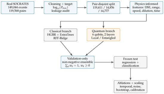
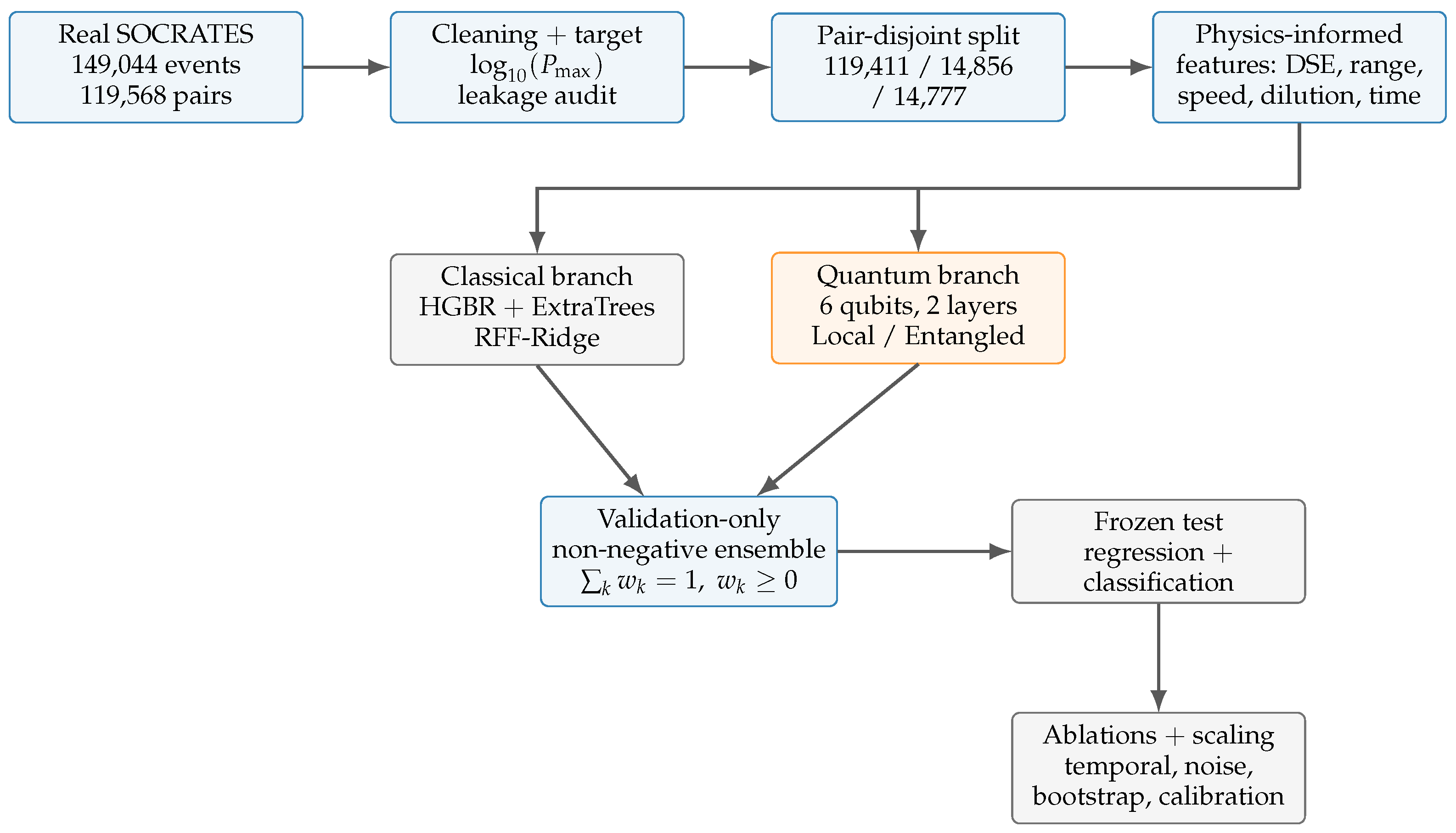
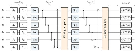
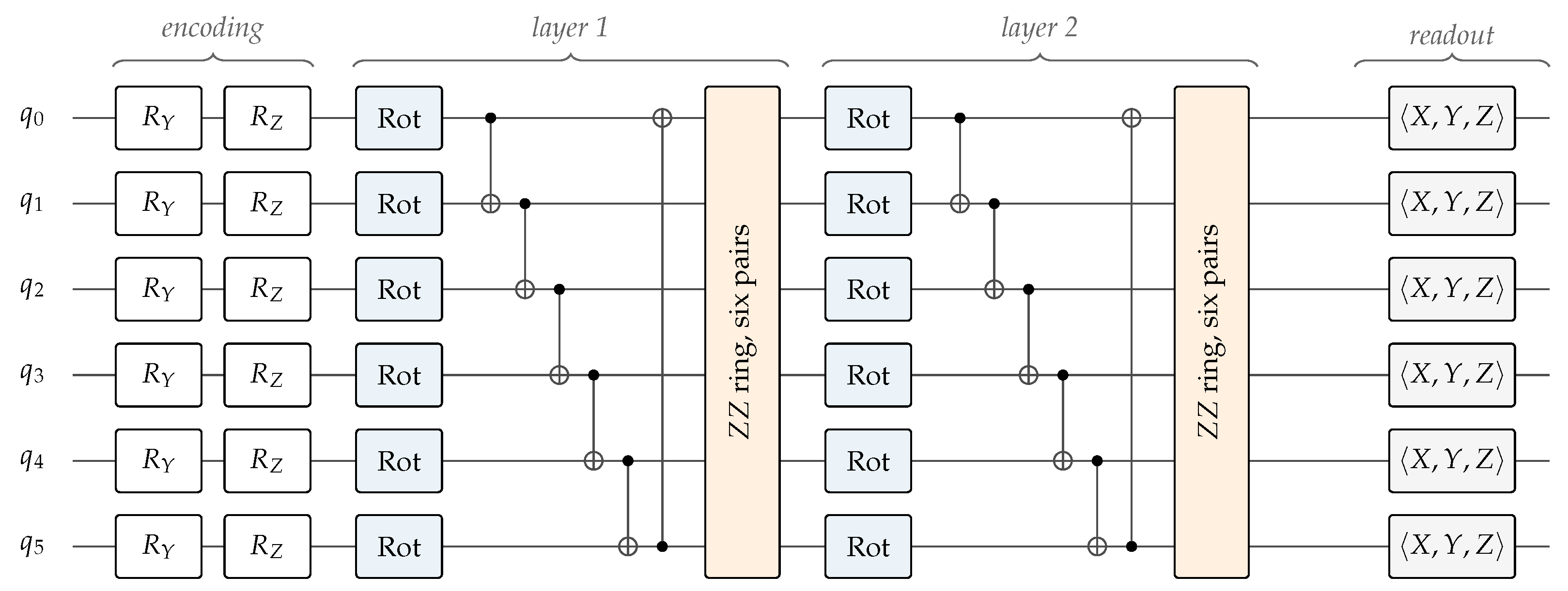
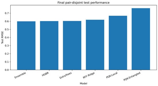
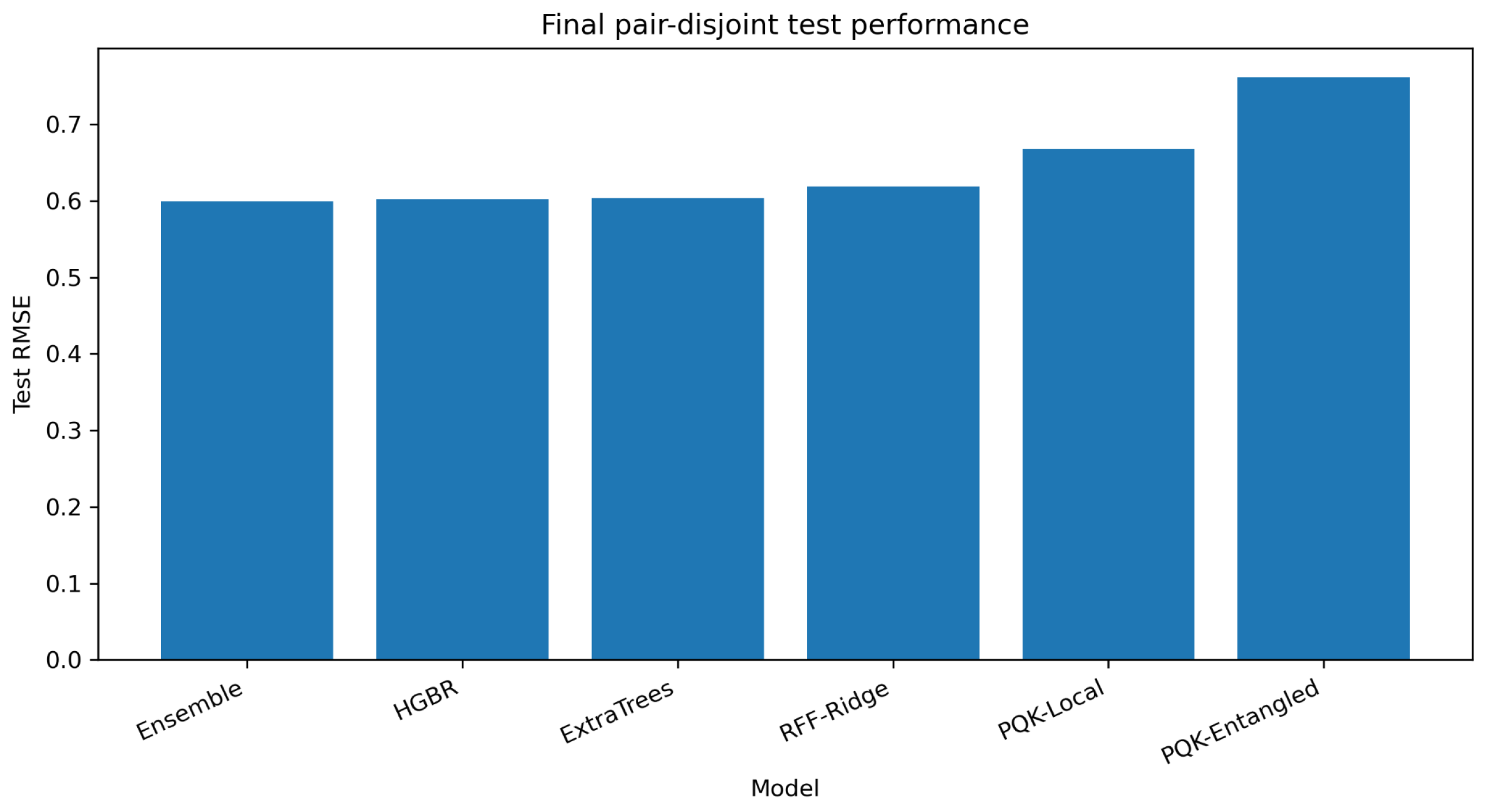
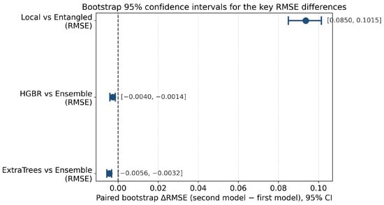
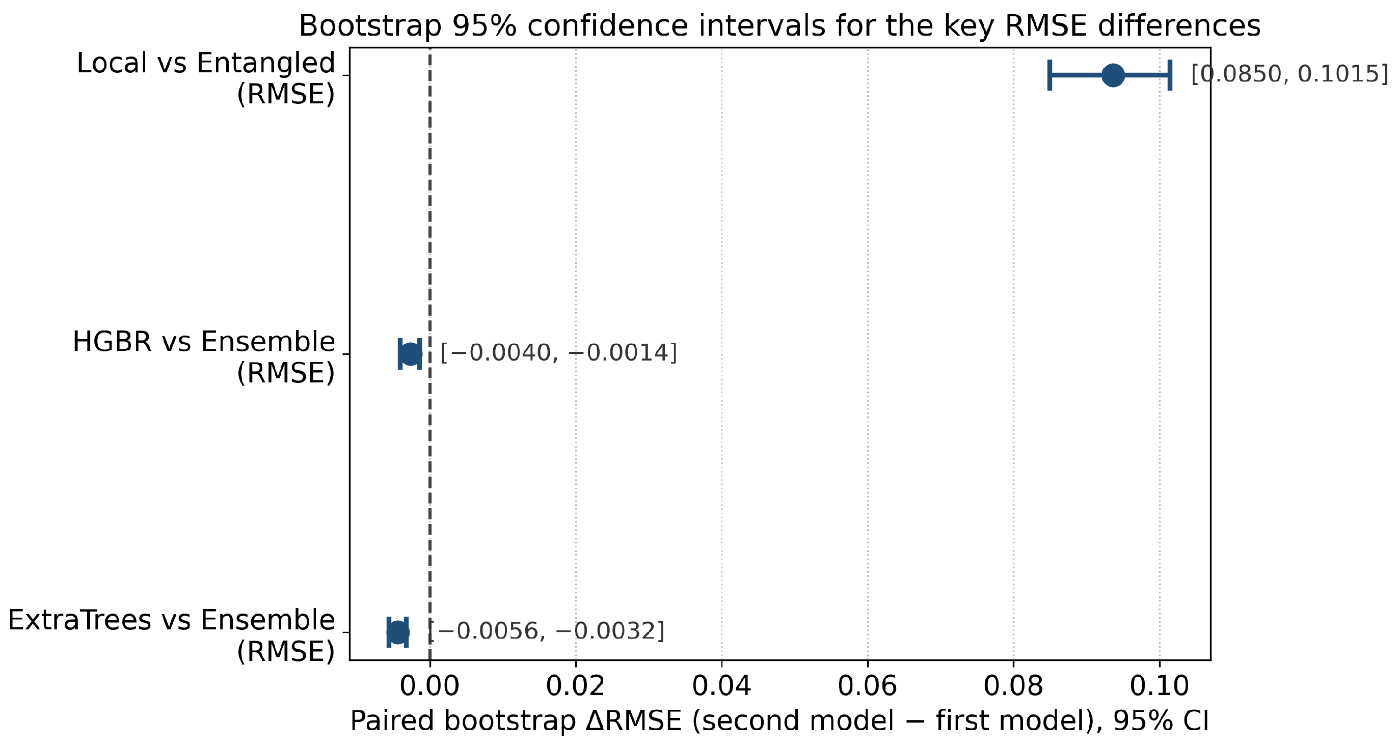
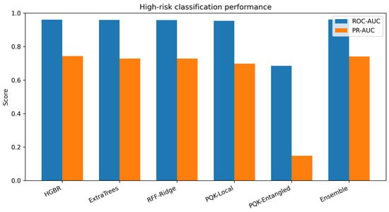
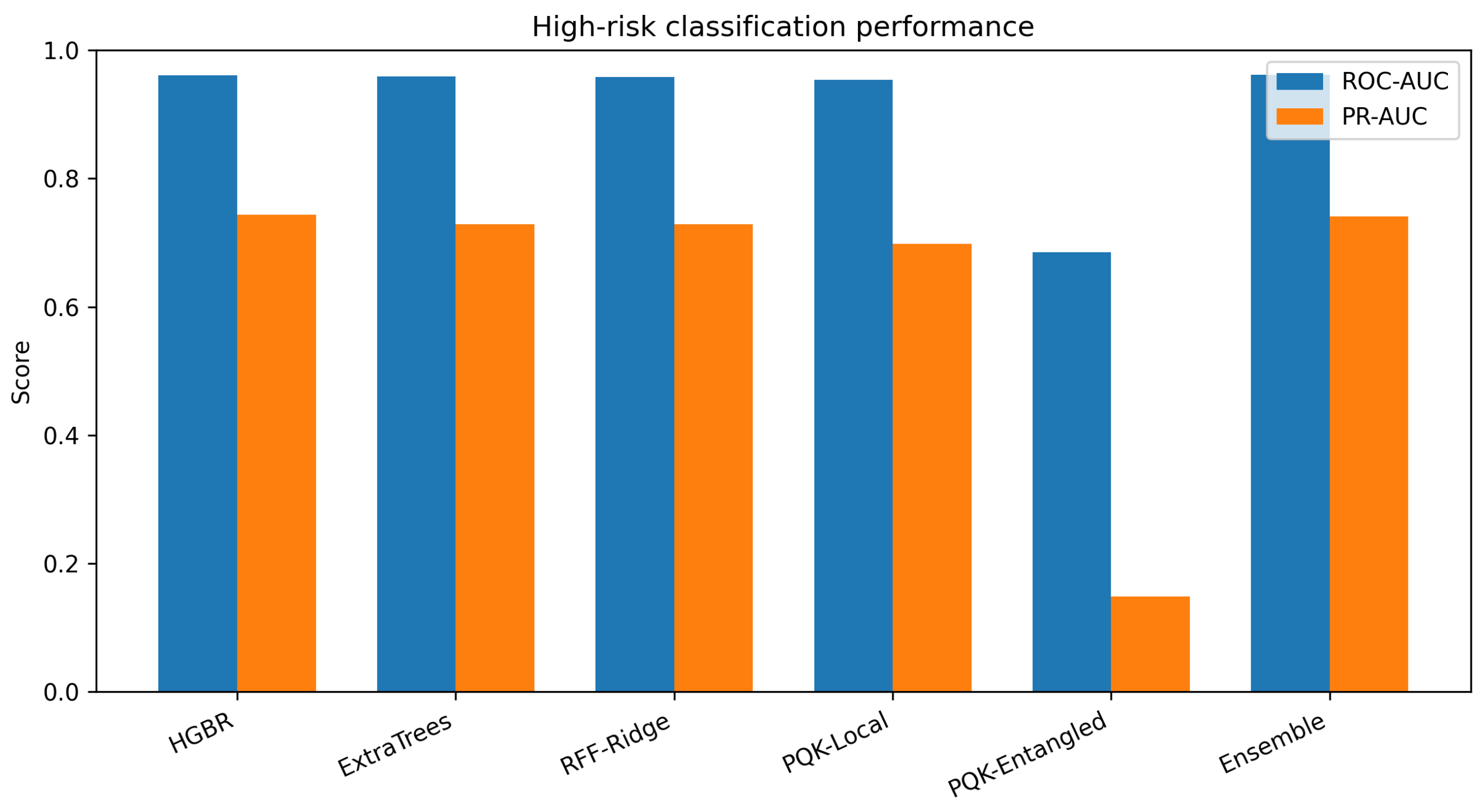
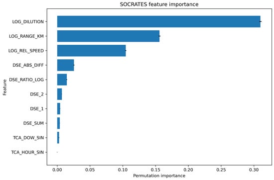
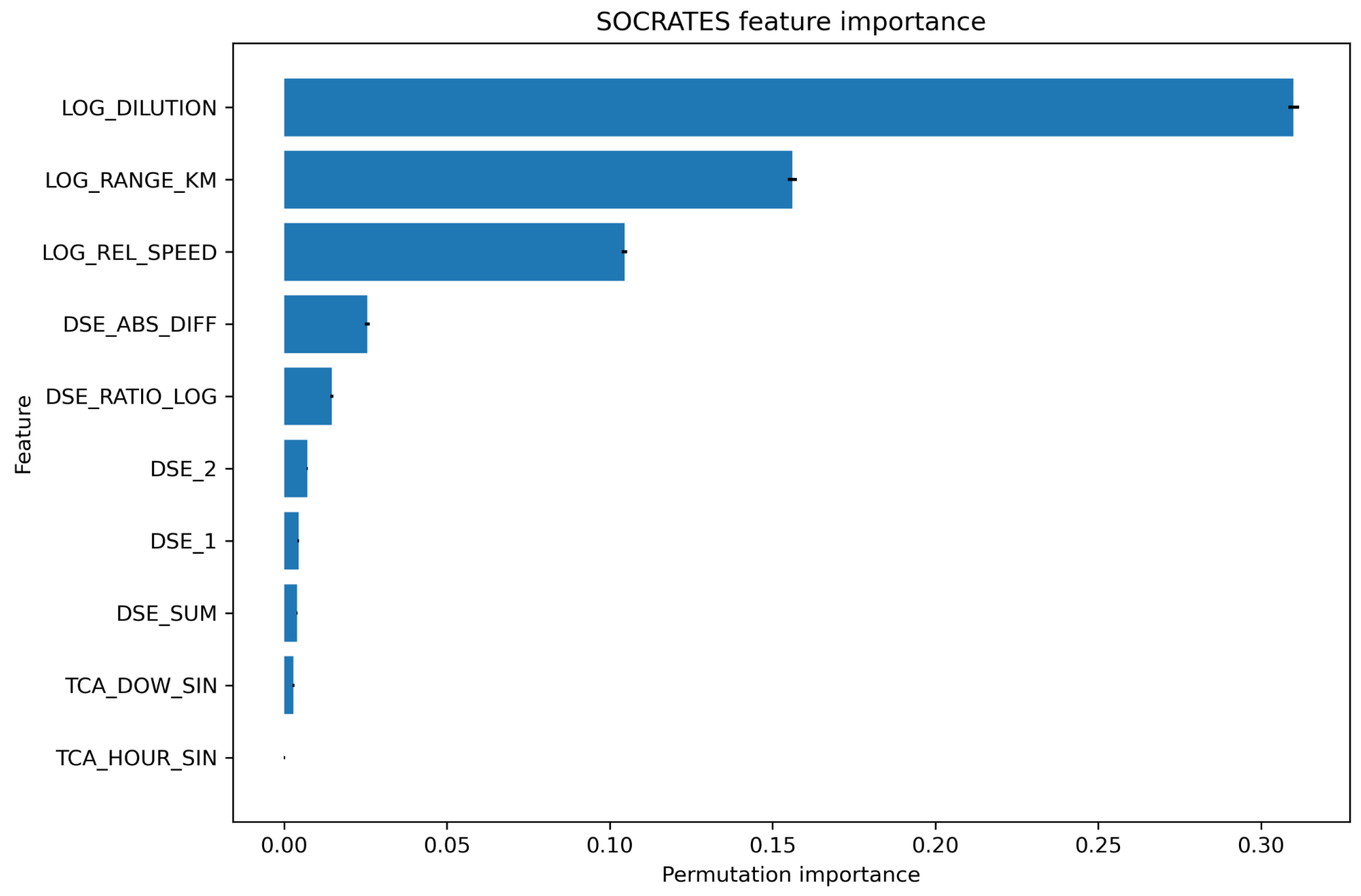
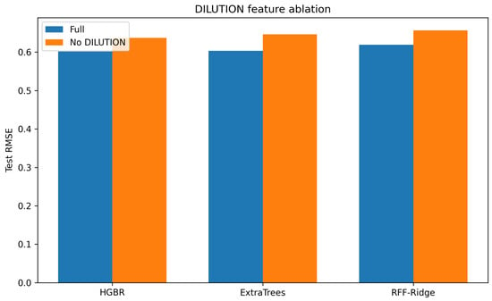
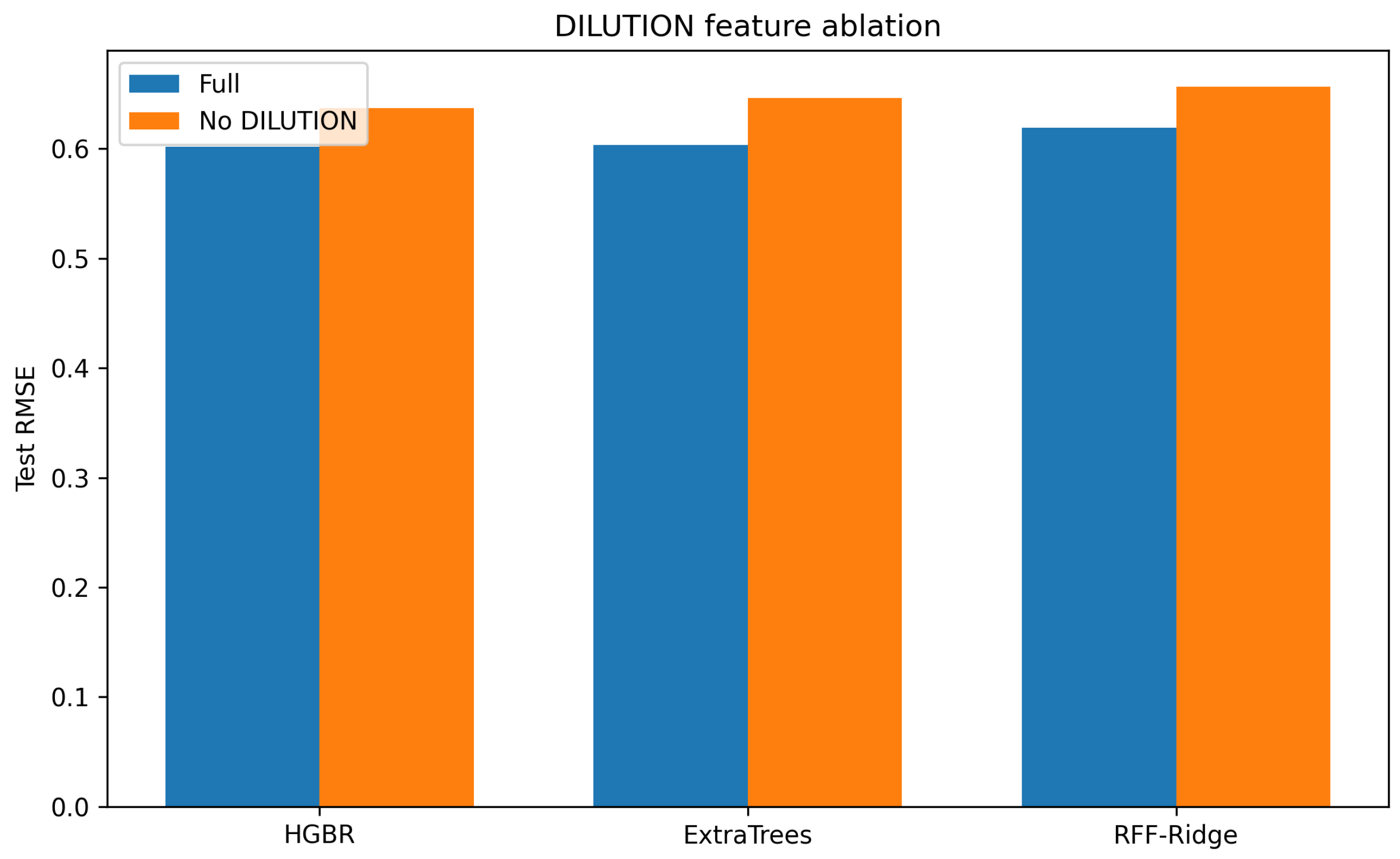
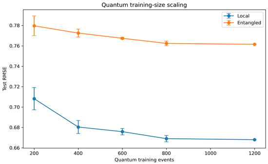
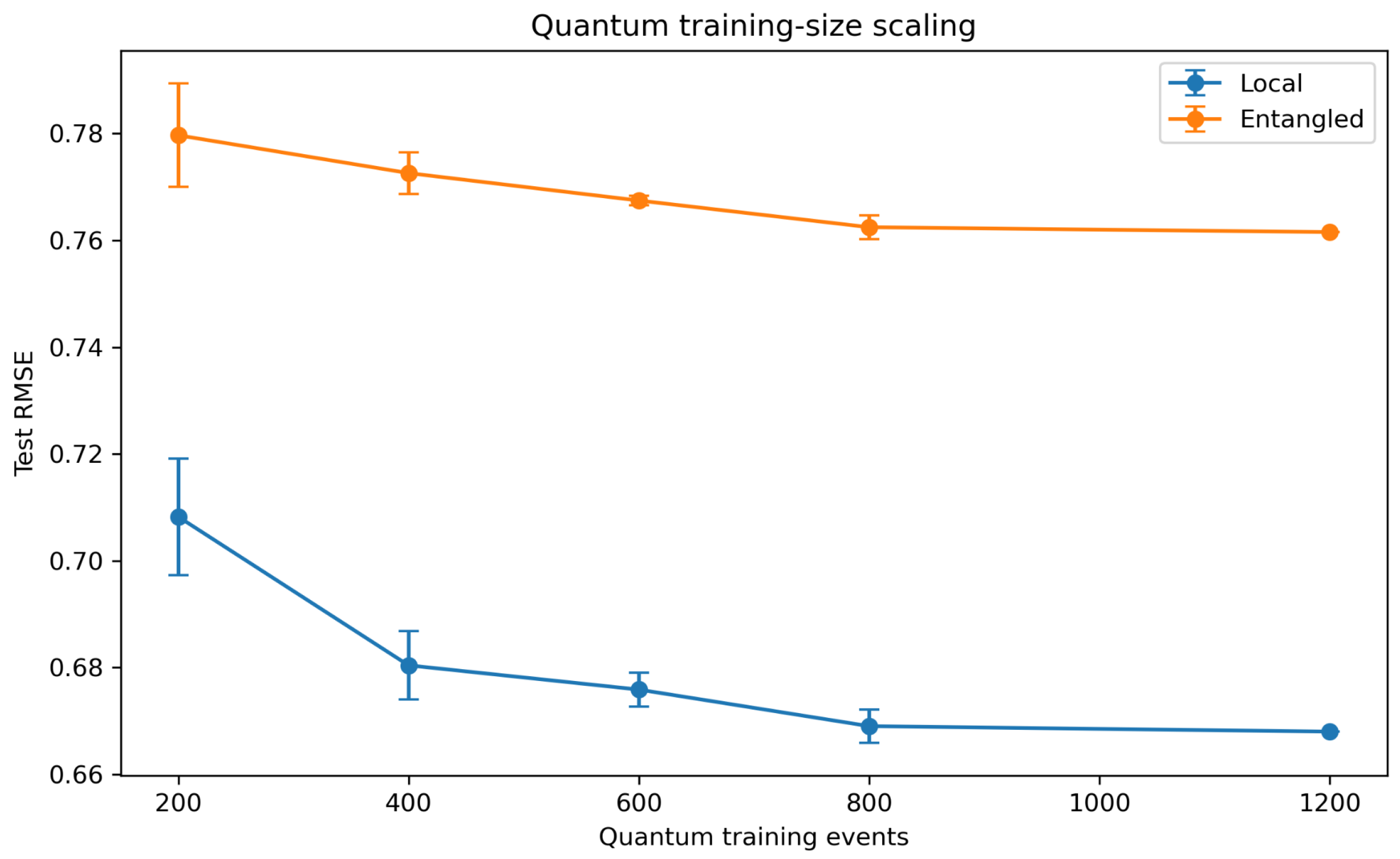
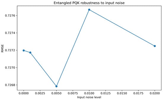
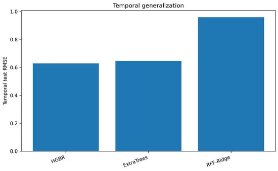
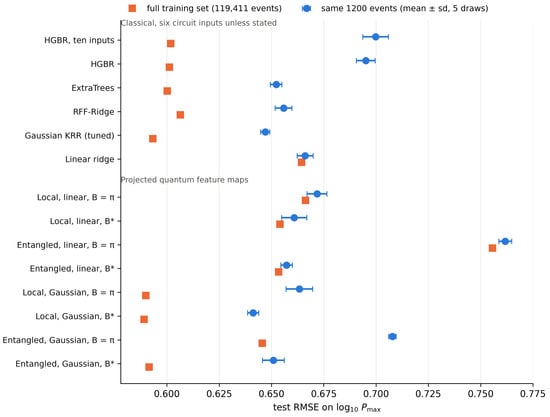
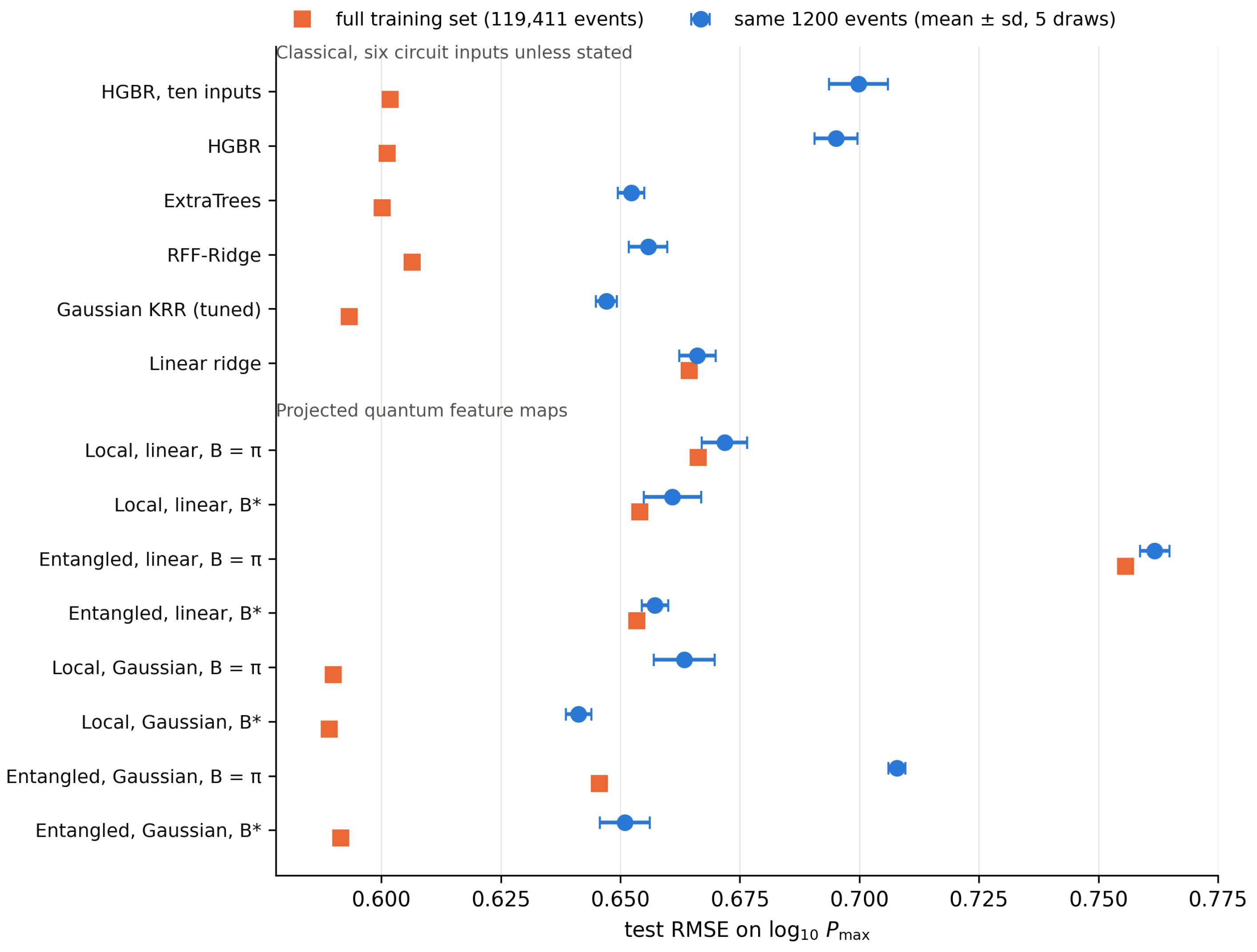
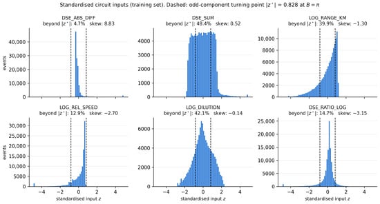
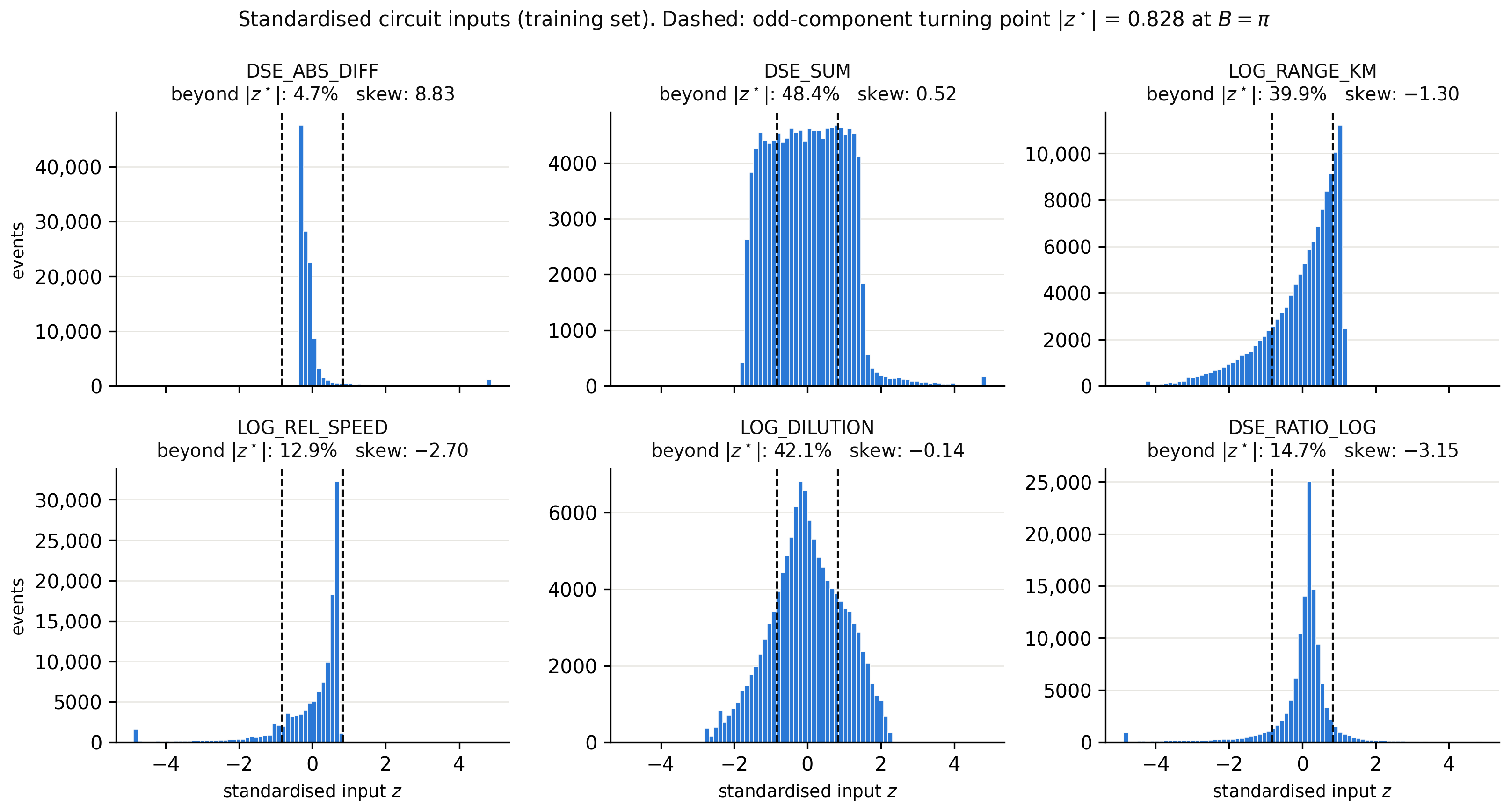

Disclaimer/Publisher’s Note: The statements, opinions and data contained in all publications are solely those of the individual author(s) and contributor(s) and not of MDPI and/or the editor(s). MDPI and/or the editor(s) disclaim responsibility for any injury to people or property resulting from any ideas, methods, instructions or products referred to in the content. |
© 2026 by the authors. Licensee MDPI, Basel, Switzerland. This article is an open access article distributed under the terms and conditions of the Creative Commons Attribution (CC BY) license.