


Abstract
This paper proposes an Improved Hybrid Gaussian Particle Swarm Optimization (IHG-GPSO) algorithm for high-dimensional global optimization. Four synergistic mechanisms are integrated: a nonlinear cosine–sine inertia weight to smoothly transition from exploration to exploitation, a memoryless random experience learning term that retains the experience-guided optimization paradigm of global PSO (GPSO) and improved PSO (IPSO) while eliminating historical optimum storage, a best-directed differential experience term inspired by differential evolution that tightens the swarm around the current global best, and a stagnation-triggered Gaussian mutation to restore population diversity without perturbing elite solutions. The proposed algorithm is evaluated on 12 classical benchmark functions at 30, 50, and 100 dimensions under a budget of fitness evaluations, and on the CEC2017 test suite with 29 functions at 10, 30, and 50 dimensions, against PSO, GPSO, IPSO, CLPSO, CMA-ES, and L-SHADE over 30 independent runs (20 independent runs for the classical functions at ). Wilcoxon rank-sum tests at show that IHG-GPSO is statistically superior or equivalent to PSO, GPSO, and IPSO on the 12 classical functions, with no case of statistical inferiority on that suite; comparisons with the contemporary optimizers CLPSO, CMA-ES, and L-SHADE show that IHG-GPSO outperforms PSO, GPSO, and IPSO on all 12 functions, while CLPSO retains an edge on selected highly multimodal functions (Rastrigin, Schwefel 2.26, Penalized 1) and CMA-ES/L-SHADE remain superior on selected unimodal cases. On CEC2017, IHG-GPSO is again the most accurate PSO-family method, attaining the best Friedman average rank among PSO, GPSO, and IPSO at all three dimensions (3.638, 3.862, and 3.621 at D = 10, 30, 50, respectively), while L-SHADE, CLPSO, and CMA-ES occupy the top of the overall ranking on most functions; statistically significant losses against them are confined to a subset of shifted and rotated problems. Convergence curves and boxplot analysis confirm faster convergence and higher stability than the PSO-family baselines, while the algorithm maintains time complexity and memory complexity, making it a lightweight and effective solver for high-dimensional optimization tasks.
Keywords:
nonlinear inertia weight; differential evolution; Gaussian mutation; particle swarm optimization MSC:
90C59
1. Introduction
Metaheuristic algorithms have become indispensable tools for solving complex global optimization problems arising in engineering design, machine learning, signal processing, and other fields, where the objective functions are often nonlinear, non-convex, multimodal, or non-differentiable. Among them, Particle Swarm Optimization (PSO), first introduced by Kennedy and Eberhart [1], stands out as one of the most popular swarm-intelligence methods, attributed to its concise principle, easy implementation, and very few tunable parameters. PSO simulates the social behavior of bird flocks or fish schools: each candidate solution in the search space is abstracted as an independent particle, which flies continuously through the search space and adjusts its velocity by referencing both the personal best position it has found in historical searches and the global best position discovered by the entire swarm, gradually approaching the global optimum through information sharing among individuals.
Despite its wide application scenarios, the standard PSO has long been recognized with two inherent drawbacks: premature convergence to local optima and rapid loss of population diversity during iterations, which become even more severe in multimodal and high-dimensional optimization landscapes. Over the past three decades, numerous improved variants have been proposed to alleviate these issues from different perspectives, and comprehensive surveys of this literature can be found in [2]. Parameter-control strategies dynamically adjust the inertia weight and acceleration coefficients to balance the global exploration and local exploitation capabilities of particles [3,4]. Topology- and learning-based improvements restructure the information flow logic within the swarm, with representative works including Comprehensive Learning PSO (CLPSO) [5], cooperative PSO [6], and bare-bones PSO [7]. Quantum-behaved models recast the particle motion rules into a probabilistic framework [8], breaking away from the fixed paradigm of traditional velocity–displacement updates. Hybrid mechanisms combine PSO with other metaheuristics, and typical combinations include the integration with Differential Evolution (DE) [9], Gaussian mutation [10], and fast evolutionary programming [11]. Clerc and Kennedy [12] also conducted a systematic theoretical analysis on the convergence behavior and parameter stability of PSO, providing theoretical support for subsequent variant designs. In recent years, novel search operators such as Lévy flight and orthogonal learning [13] have been gradually introduced into the PSO framework, further strengthening the local exploitation ability and local-optimum escaping capability of the algorithm. However, most of these improvements can only achieve performance gains on specific types of test problems. In high-dimensional multimodal complex search spaces, realizing a dynamic balance between global exploration and local exploitation remains an open challenge that has not been fully addressed in this field.
Beyond pure numerical optimization scenarios, PSO and its multi-objective extensions have been widely deployed in practical engineering systems: in power systems, for optimal siting of electric vehicle charging stations [14], optimal scheduling of cascade reservoirs [15], and edge-computing configuration for distribution-network self-healing [16]; in robotics, for inchworm climbing motion planning [17] and underwater-manipulator trajectory planning [18]; in energy and control engineering, for fractional-order PID tuning of solar-fed DC–DC boost converters [19] and wind-power fault classification [20]; and in diagnostics, for bearing fault feature selection [21,22], pneumonia detection from chest X-rays [23], and clock synchronization in cloud–edge scenarios [24]. MOPSO has also been applied to product change-scheme optimization [25], and recent surveys [26,27] confirm the wide application scope and sustained research value of the PSO paradigm. Improved population-based methods further address fuel injection quantity optimization of dual-fuel engines [28], real-time task scheduling for 3D-printing cloud platforms [29], and energy-efficient scheduling of low-carbon virtual power plants [30]. These practical demands motivate new PSO variants with higher accuracy, faster convergence speed, and stronger robustness on high-dimensional complex problems.
Among all improvement directions of PSO, a highly influential research line focuses on introducing an “experience-optimal” parameter into the velocity update rule. The Global PSO (GPSO) proposed by Jamian [31] adds a fourth update term driven by the experience-optimal vector and the improvement factor (IF). The value of is defined by randomly selecting the component of a certain dimension from the global optimum of any historical iteration. Since each iteration generates completely new experience information, particles can continuously learn from experience of different sources, which significantly accelerates the convergence of GPSO on high-dimensional problems. However, GPSO needs to store all global optima from historical iterations, which brings considerable memory overhead and drastically reduces the operational efficiency of the algorithm in extremely high-dimensional optimization scenarios. To address this limitation, Lu and Cao [32] proposed the Improved PSO (IPSO), which replaces the full-history selection rule in GPSO with a memoryless mechanism: the experience-optimal parameter is directly set to the component of a randomly selected dimension in the global optimum of the previous iteration, i.e., . Combined with the multiple random initialization strategy, IPSO effectively reduces the probability of the algorithm converging to local minima, while greatly improving the search efficiency and optimization accuracy.
In parallel, other branches of the PSO paradigm are also continuously evolving. Surrogate-assisted PSO has been developed to handle expensive constrained combinatorial optimization problems [33] and medium-dimensional expensive multi-objective optimization problems [34]. Large-scale many-objective optimizers based on Alpha-stable mutation and logistic functions have also been proposed [35]. Quantum-behaved PSO enhanced by diversity migration strategies has also been specially optimized [36]. Beyond the centralized setting, momentum-based accelerated schemes have also been developed for distributed optimization under sector-bound nonlinearity to improve the convergence rate [37]. Hybrid PSO–DE frameworks form another active branch: BBPSO-DE [38] embeds the DE mutation into the parameter-free bare-bones PSO for large-scale problems, ihPSODE [39] alternates a redesigned PSO and DE on the best half of the population to refine convergence, and LSERPSO [40] combines elitist learning with a scaling mutation and ring topology. These works mainly enrich the mutation or exemplar-selection operators. They do not, however, address the memory overhead of historical-experience learning, nor do they provide a stagnation-triggered diversity-recovery mechanism together with a rigorous stability and complexity analysis. These research advances fully demonstrate the lasting vitality of the PSO framework, but existing works are mostly designed for specific scenarios such as multi-objective optimization, large-scale optimization, or evaluation-expensive tasks. For single-objective high-dimensional global optimization, the systematic integration of the experience learning mechanism, directional differential guidance, and diversity-preserving mutation has not been fully explored, which exactly forms the core research focus of this work.
Built on the existing research foundation of standard PSO, GPSO, and IPSO, this paper proposes an Improved Hybrid Gaussian Particle Swarm Optimization algorithm, termed IHG-GPSO, which further refines the experience learning mechanism and diversity preservation mechanism. The main contributions of this work are summarized as follows:
- Nonlinear cosine–sine inertia weight. Unlike the standard linear decay, the inertia weight follows a combined cosine–sine curve that decays more rapidly through the middle iterations, promoting a faster transition from exploration to exploitation; this is paired with a mutation-based diversity-recovery mechanism for multimodal problems.
- Memoryless random experience learning term. A random experience vector is introduced into the velocity update rule, which takes the current global optimum with a predefined elite probability, and otherwise selects the personal historical best position of another randomly selected particle in the swarm. This design completely inherits the core “experience learning” idea of GPSO and IPSO, while eliminating the storage requirement for any historical optima, which fundamentally removes the extra memory overhead brought by GPSO.
- Directed differential experience term. A fourth update term is added, where and is the personal best of a randomly selected peer. This term biases particles toward the current best at a small magnitude, structurally analogous to a DE differential vector, while the diversity-recovery role is handled by the Gaussian mutation.
- Stagnation-triggered Gaussian mutation. When the global optimum has not improved for a predefined number of iterations, Gaussian perturbation with iteration-decaying amplitude is applied to all non-elite particles, which re-injects diversity into the population without disturbing the current best solution.
- Comprehensive empirical performance validation. Under the constraint of identical fitness evaluation budget, performance tests at 30, 50, and 100 dimensions are completed on 12 classical benchmark functions, with 30 independent runs for all algorithms (20 runs at ). Statistical significance comparison against standard PSO, GPSO, and IPSO is conducted via the Wilcoxon rank-sum test. The validation work is further extended to the CEC2017 standard test suite with 29 functions, covering 10, 30, and 50 dimensions, to fully verify the generality and dimension scalability of the proposed method. This paper also provides a rigorous theoretical stability and convergence analysis (stability domain of the deterministic skeleton, uniform boundedness of the clamped dynamics, a mean-square stability framework for the stochastic skeleton, and a conditional global-convergence result under recurrent stagnation-triggered mutation), convergence characteristic analysis, stability analysis based on boxplots, computational overhead analysis, and ablation experiment results that isolate the independent contribution of each mechanism.
The rest of this paper is organized as follows. Section 2 briefly reviews the core principles of standard PSO, GPSO, and IPSO. Section 3 elaborates the complete implementation details of the proposed IHG-GPSO algorithm. Section 4 describes the full setup of the experiments. Section 5 presents and discusses the experimental results on classical benchmark functions. Section 6 evaluates the performance of the proposed method on the CEC2017 test suite. Section 7 concludes the whole work.
2. Related Work
2.1. Particle Swarm Optimization (PSO)
The standard PSO first proposed in [1] initializes a swarm of N particles to explore a D-dimensional search space. For each particle i, we use and to denote its position and velocity at iteration t, respectively. The velocity and position updates for the d-th dimension follow the widely adopted rules in Equations (1) and (2):
where and are the two acceleration coefficients for the cognitive and social components, while and are independent random numbers uniformly sampled from . records the best position particle i has ever found, and is the global best solution the whole swarm has discovered so far. In practice, almost all PSO implementations use a time-varying inertia weight w [3] multiplied to the previous velocity term, as shown in Equation (3). This simple modification makes it much easier to balance the global exploration at early iterations and fine-grained local exploitation at later stages:
2.2. Global PSO (GPSO) with Improvement Factor
To bring extra diversity to the velocity update, Jamian [31] proposed the GPSO variant, which adds an experience-optimal term and defines an improvement factor (IF) to the original PSO update rule. The full velocity and position updates are written in Equations (4) and (5):
where the absolute value of the newly added fourth term is exactly the improvement factor. The term is not generated from current iteration data: instead, we randomly pick one dimension from the vector of some arbitrarily past iteration, which can be easily implemented with a Gaussian random sampling function. The original paper shows that consecutive iterations almost never get similar values, especially for high-dimensional problems. This means every particle learns from a totally different “historical experience” in each iteration, which makes GPSO converge much faster than standard PSO on high-dimensional tasks. But this design comes with an obvious downside: GPSO has to store every single historical vector, which leads to very large memory footprint and much slower runtime when the problem dimension goes very high, as pointed out in [32].
2.3. Improved PSO (IPSO) with Memoryless Experience Learning
To fix the memory overhead issue of GPSO, Lu and Cao [32] made a straightforward but effective change to the selection rule. Instead of sampling across all historical iterations, the new IPSO only uses the data from the last iteration: is set by randomly selecting one single dimension from the previous iteration’s vector:
where j is the randomly chosen dimension index. In standard PSO, the movement of each particle is completely controlled by its own personal best and the swarm global best. Once the swarm gets close to these two attractors, the search quickly slows down and gets stuck in a local optimum. The extra experience-optimal term in Equation (6) adds an unexpected perturbation to the particle’s moving direction, which often pulls it out of the local basin and increases the chance of finding the true global optimum. Besides this, IPSO also uses a multiple-random-initialization strategy: after running multiple independent sub-swarms with different random initializations, the union of all their search spaces almost covers the whole feasible region. This simple trick further reduces the probability of getting trapped in local minima, and brings clear improvements in both search efficiency and final solution precision.
2.4. Positioning Against Hybrid PSO–DE and Elitist-Learning Variants
To delimit the methodological contribution of IHG-GPSO more precisely, we contrast it with three representative recent lines of PSO redesign. First, hybrid PSO–DE algorithms such as BBPSO-DE [38] and ihPSODE [39] strengthen the mutation or refinement stage: BBPSO-DE samples new positions from Gaussian distributions centered on the personal bests and applies the DE operator to escape local basins on large-scale problems, while ihPSODE alternates a redesigned PSO and DE on the best half of the population. In both designs, the DE operator acts as a local refinement or recombination stage, and neither mechanism is coupled to a memoryless experience term of the GPSO/IPSO type. Second, elitist-learning variants such as LSERPSO [40] let particles learn from a collection of elite individuals maintained in a ring topology, with a scaling mutation to balance exploration and exploitation. Third, stagnation handling in these methods is implicit: they rely on diversity maintained by the mutation or topology rather than on an explicit no-improvement counter. In contrast, IHG-GPSO differs along three axes: (i) it inherits the GPSO/IPSO experience-learning paradigm but removes the historical-optimum storage, keeping the additional memory at ; (ii) its directed differential term is a low-magnitude best-directed guidance rather than a full DE recombination stage, and its diversity-recovery role is delegated to the Gaussian mutation; and (iii) the Gaussian mutation is triggered by an explicit stagnation counter (K consecutive iterations without global-best improvement), a design that is directly amenable to the analytical stability and convergence treatment in Section 3.8.
3. Proposed IHG-GPSO Algorithm
3.1. Motivation and Design Philosophy
We developed IHG-GPSO based on three straightforward observations we drew directly from the behaviors of standard PSO, GPSO, and IPSO in our preliminary tests. First, the overall convergence trajectory of PSO is heavily determined by its inertia weight schedule, and the widely used linear decay rule is often not optimal: in many high-dimensional multimodal problems, the swarm still needs sufficient exploration capacity in the middle and even late stages, rather than shifting to full local exploitation too early. Second, the experience-optimal mechanism in GPSO does bring very strong exploration capability, but it requires storing every historical global best, which leads to unbounded memory overhead as problem dimension grows. The memoryless selection rule in IPSO fixes this storage issue, but it also discards part of the useful historical experience information. Third, if the whole swarm is only attracted toward one single attractor, either the global optimum or a randomly sampled experience point, population diversity will quickly collapse. Adding a simple difference-based guidance term can provide a systematic directional push for particles to escape local basins, instead of relying entirely on random perturbations. Putting these three considerations together, we built IHG-GPSO by integrating four core modules: a nonlinear cosine–sine inertia weight, a memoryless random experience learning term, a directed differential experience term, and a stagnation-triggered Gaussian mutation strategy.
Table 1 positions IHG-GPSO against the compared PSO variants and representative hybrid metaheuristics along the methodological dimensions discussed above: the learning mechanism, the diversity-preservation strategy, the stagnation handling, the additional memory requirement, and the computational complexity.
Table 1.
Methodological comparison of IHG-GPSO with representative PSO variants and hybrid metaheuristics.
3.2. Nonlinear Cosine–Sine Inertia Weight
Let t denote the current iteration index, T the predefined maximum iteration budget, and the normalized progress of the optimization run. The inertia weight is updated by the following combined cosine–sine function:
At the very first iteration (), takes its maximum value , which encourages strong global exploration across the entire search space. When the run reaches the final iteration (), drops to its minimum value , supporting fine-grained local exploitation near the converged region. The factor produces a nonlinear decay that, compared with the conventional linear schedule , decreases the inertia weight more rapidly through the middle portion of the run. For example, with and , Equation (7) gives at , whereas linear decay yields . This faster reduction accelerates the transition toward local exploitation on smooth landscapes; on multimodal functions where early exploitation may prematurely narrow the search, the stagnation-triggered Gaussian mutation re-injects diversity when the swarm stalls. We emphasize that the schedule depends only on the iteration count and not on live swarm state; it is therefore a predetermined nonlinear decay rather than a truly state-adaptive weight.
3.3. Random Experience Learning Term
We keep the core experience-optimal idea from GPSO and IPSO, but redesign it completely in a memoryless way, so that no historical optimum needs to be stored at all. For each particle in every iteration, we generate a random experience vector . We first sample a uniform random particle index q that satisfies , to make sure we never sample the target particle itself. The value of is then selected by Equation (8):
where is a predefined elite probability. With probability , the particle is attracted toward the current global best to perform focused local exploitation; otherwise, it is guided by the personal best of a randomly selected peer particle, to enforce more diverse global exploration. This design fully retains the performance advantage of experience learning, while completely eliminating the memory overhead for historical optimum storage. The random peer selection also naturally injects extra diversity into the social learning phase of the algorithm.
3.4. Directed Differential Experience Term
To further strengthen the local-optimum escaping ability, we add an extra directed differential term into the velocity update rule. We set and , where q is again a uniformly sampled random particle index. The corresponding new velocity component is written as in Equation (9):
This term biases each particle’s velocity toward the current global optimum relative to a peer’s personal best, which geometrically accelerates convergence toward the elite region. It shares a structural resemblance with the differential mutation operator in differential evolution (DE) [9,41], but we note that because , the net effect is primarily exploitative rather than exploratory: it tightens the swarm around the current best while the small coefficient limits its magnitude so that it does not dominate the cognitive and social terms. The exploration-recovery role is instead delegated to the stagnation-triggered Gaussian mutation described below.
3.5. Stagnation-Guided Gaussian Mutation
We calculate population diversity using the normalized mean Euclidean distance from all particles to the swarm centroid, as defined in Equation (10):
where is the centroid of the current swarm, and , are the upper and lower bounds of the search space, respectively. We use this diversity measure diagnostically (see the diversity-trajectory analysis in Section 6.8) rather than as part of the mutation trigger. The mutation is activated only when the global best has not improved for K consecutive iterations; because the acceptance test uses a very tight tolerance, this occurs exclusively when the swarm has truly frozen, i.e., no particle produces any numerically better fitness for K consecutive iterations. As documented in Section 6.8, in representative runs under the standard budget this condition is not reached, since the random experience and differential terms keep producing small fitness improvements that reset the stagnation counter; the mutation therefore acts as a conservative safety net for fully frozen swarms rather than as a scheduled diversity operator. Under this condition, we apply a Gaussian perturbation to all particles except the one carrying the current global best:
where is the normalized initial mutation amplitude, is the component-wise width vector of the box , and gradually decays to zero as the iteration count increases; for the hypercube benchmark domains used in this paper, all per-dimension widths coincide, so is a scalar ( for every j) and the covariance in (11) is . The global-best particle is always excluded from this perturbation, so we never risk losing the best elite solution we have found so far. After the Gaussian mutation is applied, we reset the stagnation counter to zero to restart the accumulation of improvement records.
3.6. Complete Algorithm
Putting all the above components together, the full velocity–position update rule of IHG-GPSO is written as
After each position update, we apply simple boundary clamping to keep all particles inside the feasible search domain: . We also enforce velocity clamping to avoid excessive step size, with , so that . The full step-by-step procedure of IHG-GPSO is summarized in Algorithm 1, and the overall search mechanism is intuitively illustrated in Figure 1.
| Algorithm 1 IHG-GPSO |
|
Figure 1.
Flowchart of the proposed IHG-GPSO algorithm. In the flowchart, asterisks denote multiplication.
3.7. Computational Complexity
We derive the complexity of IHG-GPSO by a direct operation count per iteration. Within one iteration, each of the N particles executes the following elementary operations: (i) sampling two peer indices (); (ii) forming the random experience vector and the differential pair , each requiring an vector copy; (iii) the velocity and position updates (13), which require arithmetic operations per particle; and (iv) one fitness evaluation of cost for the benchmark landscapes used in this paper. The stagnation counter is , and the conditional Gaussian mutation costs per trigger and fires at most once per iteration. Summing over the swarm and over the iteration budget T gives
which is of the same order as standard PSO and introduces no extra asymptotic overhead; the additional experience-sampling and differential operations contribute only constant factors. In terms of memory, IHG-GPSO stores the positions, velocities, and personal bests ( doubles), the current global best (D doubles), and a constant number of scalars, so
Because no historical optima are stored, the memory footprint does not grow with the iteration count; in contrast, GPSO retains the full global-best vector of every past iteration and hence scales as , and CMA-ES maintains a covariance matrix and scales as in memory and per generation for the eigen-decomposition of the covariance matrix.
To quantify this advantage, Table 2 lists the theoretical memory footprint of all compared algorithms.
Table 2.
Theoretical complexity and measured runtime/memory of all compared algorithms. Wall-clock time is measured on the antenna pattern-synthesis problem (, , , averaged over 5 runs) with the identical MATLAB R2024a platform and vectorized implementation style; the memory column is the analytical footprint of the main state variables (doubles).
The memory of IHG-GPSO is doubles (positions, velocities, personal bests, and current global best), whereas GPSO requires doubles because it retains the entire history of global-best vectors over T iterations. The ratio is independent of D:
for , , which is the theoretical worst-case peak ratio under full-history storage. The measured peak memory footprint in Table 2 is , slightly below this bound because the historical archive is stored as a pre-allocated matrix in our MATLAB implementation. Regardless of the exact constant, the advantage grows with the iteration budget T (the ratio is asymptotically proportional to ) and is independent of the dimension D.
CMA-ES stores a covariance matrix, giving memory, and requires an eigendecomposition of this matrix together with the -weighted covariance update each generation, giving per-generation time complexity, compared with for IHG-GPSO. The crossover point where CMA-ES exceeds IHG-GPSO in memory is , i.e., . Below this dimension, CMA-ES is more memory-efficient; above it, IHG-GPSO’s linear scaling becomes advantageous. At , the per-generation cost of CMA-ES is roughly times the per-iteration cost of IHG-GPSO, a ratio that grows quadratically with dimension.
To verify the derived scaling numerically rather than relying on the asymptotic analysis alone, Table 3 reports the measured wall-clock time of PSO, IHG-GPSO, and CMA-ES on the Sphere function (, averaged over three runs, identical MATLAB R2024a platform and vectorized implementation style) for increasing N and D. Three facts confirm the derivation. First, for a fixed population (), the runtime of IHG-GPSO grows linearly with D: increasing D from 30 to 200 () raises the time from s to s (). Second, for a fixed dimension (), increasing N from 50 to 200 () raises the time from s to s (), close to the linear prediction. Third, CMA-ES exhibits a clearly super-linear growth with the dimension: from to (), its time grows from s to s (), in line with the – covariance operations. The constant overhead of IHG-GPSO relative to standard PSO stays in the narrow band – across all tested settings (Table 3), which confirms that the two added mechanisms do not change the order of growth and only contribute a small, dimension-independent constant factor.
Table 3.
Measured wall-clock time (s) of PSO, IHG-GPSO, and CMA-ES on the Sphere function (, averaged over 3 runs, MATLAB R2024a, vectorized implementations). The last column is the constant overhead of IHG-GPSO relative to standard PSO.
3.8. Stability and Convergence Analysis
This subsection provides a rigorous theoretical characterization of the stability and convergence behavior of IHG-GPSO. We proceed in four steps: (i) we analyze the deterministic skeleton of the velocity–position dynamics and derive its stability domain via the Jury criterion; (ii) we establish the boundedness of the state trajectory under the velocity and boundary clamping used in Algorithm 1; (iii) we establish a mean-square stability framework for the stochastic skeleton with random coefficients; and (iv) we prove a global-convergence result that is conditional on the recurrent firing of the stagnation-triggered mutation and that exploits the elite-preservation property and the stagnation-triggered Gaussian mutation.
3.8.1. Deterministic Skeleton and Its Stability Domain
Following the standard approach of Clerc and Kennedy [12] and Trelea [42], we first study the deterministic skeleton obtained by fixing the attractors and replacing the random coefficients by their expectation. Consider a single particle attracted to a fixed point p with the composite update
where and are constant. Let and , and define the displacement . Then, (17) is equivalent to the linear state-space recursion with and
Under the dynamics (17), the particle converges to the attractor p (i.e., ) for every initial state if and only if
Proof.
The characteristic polynomial of A is . A second-order discrete linear system is asymptotically stable if and only if the Jury conditions hold: , , and . We verify each condition. First, because . Second, , so is equivalent to . Third, is exactly the first condition in (19). Conversely, if any condition in (19) fails, at least one eigenvalue of A lies on or outside the unit circle, so the origin is not asymptotically stable. This completes the proof. □
Remark 1.
For the parameters used in this paper, (hence ) and decreases monotonically from to . The deterministic stability condition (19) holds whenever . Solving with the cosine–sine schedule (13) gives , i.e., . Hence, the deterministic skeleton is asymptotically stable during approximately the first of the run, i.e., exactly the exploration phase during which a high inertia weight is required. In the remaining part of the run, one eigenvalue of the unclamped skeleton leaves the unit circle and the free dynamics diverge; however, the state trajectory remains bounded by the velocity and boundary clamping of Lemma 1; the homogeneous first-moment operator , whose attractor coefficient is , is Schur-stable for every , since the Jury condition , i.e., , holds for all ; the first-moment trajectory is hence bounded and contracts toward the attractor once the driving terms vanish. The mean-square condition of Theorem 1 is active for the adopted acceleration coefficients: for , numerical evaluation of the closed-form second-moment matrix reported before Theorem 1 gives for all and for all , with at ; the homogeneous stochastic skeleton is therefore mean-square stable for and mean-square unstable for . Since the cosine–sine schedule (13) starts at and crosses at , the first of the run operates in the mean-square-unstable regime, whereas the remaining is mean-square stable; the velocity and boundary clamping of Lemma 1 keeps the clamped trajectory bounded in both regimes. Mean-square contractivity is likewise obtained for small acceleration coefficients: for , one has for (with at ), again verified numerically from the same closed-form matrix. Consequently, the operative stability guarantees of IHG-GPSO under the adopted parameters are (i) the asymptotic stability of the deterministic skeleton for , (ii) mean-square stability for (covering the last of the run), (iii) the almost-sure boundedness of Lemma 1, (iv) first-moment contraction over the whole run, and (v) the extensive numerical validation reported in Section 5. This explains why the aggressive cosine–sine decay is beneficial: it keeps the swarm inside the deterministic stability domain during exploration, where uncontrolled oscillations would be harmful, and then transfers the dynamics into a regime of small w in which the velocity term decays quickly and the swarm performs a bounded, contraction-dominated local refinement, while the Gaussian mutation re-injects diversity if the swarm freezes.
3.8.2. Boundedness of the Clamped Dynamics
Lemma 1.
Under the velocity clamping and the boundary clamping applied in Algorithm 1, every trajectory generated by IHG-GPSO satisfies and for all and all i.
Proof.
We proceed by induction on t. At , the initialization and satisfies the claim. Assume the claim holds at time t. Step 10 of Algorithm 1 computes by (13) and then applies the coordinate-wise projection , which yields . The position is then updated and projected as , which yields . Hence, the claim holds at , and the induction is complete. □
Lemma 1 guarantees that the state trajectory remains in the compact set regardless of parameter settings; in particular, the potential instability of the unclamped skeleton in the late iterations (Remark 1) cannot lead to unbounded divergence.
3.8.3. Mean-Square Stability of the Stochastic Skeleton
We now consider the stochastic skeleton in which are independent and the elite attractor and the differential pair are random but bounded. The external driving terms are collected into . Because are personal-best or global-best vectors, all of which lie in , and is a convex combination, there exists a constant such that almost surely for all t. The stochastic recursion reads
where is obtained from A by replacing with , and .
Let be the second-moment operator of the homogeneous part, defined with respect to the row-major vectorization by , a matrix whose entries are polynomials in w and in the moments , . This is the exact operator of the vectorized second-moment recursion: since are independent of , the -entry of equals . By the stochastic stability theory of PSO [42,43], the homogeneous recursion is mean-square stable if and only if . For completeness, we report the closed-form second-moment matrix. With , , and , and the row-major ordering , the entries of are
For the parameters used in this paper (), numerical evaluation of the closed-form matrix above gives for all and for all , with at : the skeleton is mean-square stable for and mean-square unstable for , so the mean-square criterion is active under the adopted acceleration coefficients. Since the cosine–sine schedule crosses at , the first of the run lies in the mean-square-unstable regime, whereas the remaining iterations are mean-square stable; the velocity and boundary clamping of Lemma 1 keeps the clamped trajectory bounded in both regimes. For smaller acceleration coefficients, the stable interval widens: for , for (the boundary value at which is , as verified numerically from the closed-form matrix above). The framework of Theorem 1 therefore applies to the mean-square-stable regime of the adopted schedule, while the stability of the early unstable regime and of the clamped dynamics rests on the deterministic Jury condition, the boundedness lemma, first-moment contraction, and numerical validation; see Remark 1.
Theorem 1.
Let be the second-moment operator of the homogeneous stochastic skeleton (20) and assume . Then, there exist constants and such that, for the stochastic recursion (20),
where is the almost-sure bound of Lemma 1. If the external driving terms vanish (), the mean square error converges to zero exponentially:
for some constant .
Proof.
Let and . Since are independent of and of the driving terms, vectorizing the recursion (20) yields the exact second-moment recursion
where
collects the cross and external second-moment terms. Because by assumption, there exists a matrix norm such that (take the norm induced by the Lyapunov solution of the discrete Lyapunov equation). By Lemma 1, the state is almost surely bounded, ; by construction, the driving term satisfies almost surely. Let . The cross terms are bounded via Cauchy–Schwarz as
and . Hence, there is a constant depending only on the parameters and on R such that for all t. Iterating (23) in the Lyapunov norm gives
Theorem 1 establishes the mean-square framework for the stochastic skeleton: whenever the second-moment operator is contractive, the expected squared distance from any fixed attractor cannot grow without bound, and in the absence of external driving, it contracts exponentially. Under the acceleration coefficients adopted in this paper, the mean-square condition is active in the stable regime of the inertia schedule (, covering the last of the run; see Remark 1); the operative guarantees are the deterministic Jury condition, the boundedness lemma, first-moment contraction, mean-square stability in the stable regime, and the numerical evidence in Section 5. The additive term reflects the fact that the attractors themselves keep moving as the swarm improves, which is precisely the desired behavior of an adaptive search.
3.8.4. Global Convergence via Elite Preservation and Stagnation-Triggered Mutation
Following the classical random-search convergence framework of Solis and Wets [44], we analyze the global-convergence behavior of IHG-GPSO. The result is necessarily conditional: the mutation mechanism fires only when the swarm stagnates, so the hitting probability is expressed in terms of the (random) number of stagnation-triggered mutation events. Let f be continuous on the compact box and let . For define the -optimal set . By continuity of f, the set contains a neighborhood of a global minimizer intersected with ; hence, it has positive Lebesgue measure. Let denote the number of stagnation-triggered mutation events that have occurred up to iteration t.
Theorem 2
(Conditional global convergence). Consider IHG-GPSO (Algorithm 1) with particles, iteration budget T, and the elite-preservation rule (the global-best carrier is never mutated, and is updated only upon improvement). Assume that:
- (A1)
- the objective f is continuous on the compact box ;
- (A2)
- for a fixed , the mutation amplitude satisfies for every dimension j at every trigger time ;
- (A3)
- by iteration , the stagnation-triggered mutation has fired times.
Then, for every ,
where and is a uniform lower bound on the probability that a single mutated particle lands in at any trigger time .
Proof.
Fix . Whenever the mutation trigger fires, every particle except the global-best carrier is independently perturbed according to (11) and (12), i.e., with and for every dimension j and . The probability that a single mutated particle falls into is
where is the D-dimensional Gaussian density. Fix . On the finite horizon , the mutation amplitude satisfies for every dimension j. Because is compact, the Gaussian density admits a uniform positive lower bound on over this horizon; combined with , this gives for all i and all trigger times . The perturbed particles are drawn independently, so the probability that a single trigger fails to place any particle in is at most with . Conditioning on the history up to each trigger and using the chain rule of conditional probability, each trigger has conditional success probability at least , so the probability that all of the first triggers fail is at most . Whenever a trigger succeeds, the mutated particle’s fitness enters the -optimal level, and the elite-preservation rule of Algorithm 1 guarantees that the global best is never worsened (the best particle is excluded from mutation and is updated only upon improvement). Therefore, permanently from the first successful trigger onward, which proves (27). □
Remark (scope of the claim). Theorem 2 is a conditional convergence result: it bounds the hitting probability from below by a quantity that grows to one exponentially in the number of stagnation-triggered mutation events. It does not assert that the algorithm dynamics generate infinitely many such events. Whether on a given run depends on the stagnation pattern of that run; it can fail, for example, when the swarm keeps producing small improvements so that the stagnation counter never reaches K, in which case, the Gaussian mutation does not fire at all (as observed in the sensitivity and diversity analysis of Section 6.8). Accordingly, the theorem should be read as a conditional global-convergence statement under recurrent mutation, in the spirit of Solis and Wets [44]; it neither claims that a finite budget T guarantees hitting the global optimum nor that recurrent mutation occurs almost surely under the algorithm dynamics. This is consistent with the empirical convergence curves reported in Section 5, where the mutation mechanism is observed to restore progress on multimodal functions after periods of stagnation.
4. Experimental Setup
4.1. Benchmark Functions
We directly adopt 12 standard benchmark functions from the well-known classical test suite proposed by Yao et al. [11], which has been widely used in the metaheuristic optimization community for decades and guarantees strong result comparability across different studies. The selected test set covers four pure unimodal functions –, which are designed to verify the local convergence speed and exploitation precision of the algorithm. The Rosenbrock function is also included, whose global optimum is hidden inside a long, narrow, curved valley. This tricky landscape easily traps algorithms into oscillating around the valley edge, making it extremely hard to locate the true global optimum. The remaining seven functions – are all multimodal, with a large number of local optima distributed across the feasible domain, which specifically examines the algorithm’s ability to escape local basins and maintain stable global exploration. All functions are uniformly shifted, so that their theoretical global optimum values are normalized to zero for direct and fair convergence accuracy comparison. Table 4 lists the search range and category of each benchmark function, and Appendix A (Table A1) gives the exact mathematical formulations, including the penalty factors of the shifted/penalized variants, so that no ambiguity remains. All comparative tests are conducted under three different dimensions, , , and , to validate the performance consistency of the proposed algorithm across different problem scales.
Table 4.
Benchmark functions used in the experiments.
4.2. Parameter Settings
To ensure a fair comparison, all seven algorithms share the same population size, evaluation budget, and common parameters; algorithm-specific coefficients follow their respective designs in the literature. The settings are summarized in Table 5.
Table 5.
Parameter settings of the compared algorithms.
4.3. Statistical Methodology
We run every algorithm for 30 completely independent trials on each pair of benchmark function and dimension setting. During each single run, we log the best-so-far fitness value at every iteration step, and store the final best fitness obtained when the run terminates. After collecting results from all 30 independent runs, we calculate and report the mean, standard deviation, best, worst, and median of these final fitness values for each algorithm. To check whether the performance gap between IHG-GPSO and each competing method is statistically meaningful rather than caused by random luck, we conduct a two-sided Wilcoxon rank-sum test with the significance level set to . In the result tables, we use the symbols “+”, “−”, and “=” to mark the statistical outcome: “+” means IHG-GPSO performs significantly better than the corresponding competitor, “−” means IHG-GPSO is significantly worse, and “=” indicates no statistically significant difference between the two methods. To guarantee full experimental reproducibility for any follow-up verification, we assign a fixed pre-defined random seed to every single (function, dimension, algorithm, run) combination, so that all random sampling processes in the algorithm are fully deterministic.
5. Results and Discussion
5.1. Optimization Accuracy at
The mean and standard deviation of the final fitness values over 30 independent runs for all compared algorithms under are summarized in Table 6. Within the PSO family (PSO, GPSO, IPSO, and IHG-GPSO), the proposed method stands out clearly: it obtains the best mean accuracy on all 12 benchmark functions without a single exception, and its standard deviations are generally much smaller than those of the PSO baselines, confirming stable and reliable performance across independent runs. The gains over the three PSO baselines are particularly noticeable on the unimodal functions – and the Rosenbrock function : for example, on the Sphere function , IHG-GPSO reaches a mean fitness of , about 26 orders of magnitude better than standard PSO () and vastly superior to GPSO (). On the multimodal functions, IHG-GPSO also consistently beats the PSO baselines by a clear margin; e.g., on Rastrigin , its mean fitness of 28.04 compares with 43.78 (PSO), 179.70 (GPSO), and 50.59 (IPSO), and on Ackley , it reaches , essentially the floating-point machine precision.
Table 6.
Mean ± std of final fitness over 30 runs at . Best results in bold.
When the comparison is extended to the three contemporary optimizers, the picture becomes more nuanced and, in our view, more informative. CMA-ES attains the best mean accuracy on the separable unimodal functions (, , ), on Rosenbrock, and on Ackley; L-SHADE is the best on Schwefel 2.22, Weierstrass, and both penalized functions; and CLPSO delivers the lowest mean errors on the strongly multimodal Rastrigin, Griewank, and Schwefel 2.26 functions, where its comprehensive-learning strategy is particularly effective. IHG-GPSO remains the strongest PSO-family method on every function and stays within approximately one order of magnitude of the best modern optimizer on Ackley and on Weierstrass, while on Penalized 1, it approaches machine precision () and trails L-SHADE by a marginal factor of about 1.1. This shows that the proposed hybrid design narrows the gap between the classical PSO paradigm and modern covariance-matrix- or adaptive-differential- evolution-based optimizers on most landscape types.
5.2. Optimization Accuracy at
We list the full set of comparative results for the high-dimensional setup in Table 7. Within the PSO family, IHG-GPSO still outperforms PSO, GPSO, and IPSO on all 12 benchmark functions, with no single case left behind, and the gaps between IHG-GPSO and the other three PSO methods generally grow with the dimension: for example, on Sphere, the mean fitness improves from at to at for IHG-GPSO, whereas standard PSO degrades from to , and on Rastrigin, the IHG-GPSO mean of 69.55 clearly beats PSO (128.49) and IPSO (120.48). These results confirm that the random experience learning and the directed differential term remain effective as the problem dimension grows.
Table 7.
Mean ± std of final fitness over 30 runs at . Best results in bold.
With respect to the three contemporary optimizers at , CMA-ES again dominates the separable unimodal landscape and Rosenbrock; CLPSO keeps the lead on Rastrigin, Schwefel 2.26, and Penalized 1; and L-SHADE remains the best on Schwefel 2.22, Weierstrass, and Penalized 2. IHG-GPSO preserves its status as the strongest PSO-family optimizer, and its accuracy relative to the best modern method degrades only mildly with dimension on the multimodal cases (e.g., on Rastrigin, the mean error grows from 28.0 at to 69.5 at , a factor of about 2.5, versus factors of about 2.0 for CMA-ES and 10.1 for CLPSO, whose exceptionally strong accuracy of 4.46 deteriorates more rapidly), indicating that the proposed mechanisms scale reasonably well to higher dimensions.
5.3. Statistical Significance
Table 8 aggregates all pairwise Wilcoxon rank-sum test results between IHG-GPSO and each competing algorithm, calculated from the 30 independent runs on every test case. Because twelve functions and six competitors produce multiple simultaneous comparisons per dimension, the raw p-values are adjusted with the Holm–Bonferroni procedure per function, and the effect size of every comparison is quantified with the rank-biserial correlation (all significant cases in Table 6 and Table 7 carry , i.e., at least a large effect). The complete per-function p-values and effect sizes of every pairwise comparison at both dimensions are tabulated in Appendix A (Table A2). Within the PSO family, the result is very solid: across both and setups, IHG-GPSO never shows a statistically worse performance than PSO, GPSO, or IPSO on any benchmark function. Against GPSO, IHG-GPSO secures significant wins on all 12 functions at both tested dimensions. Against standard PSO, it records 9 wins and 3 ties at and 10 wins and 2 ties at ; against IPSO, the counts are 8 wins/4 ties at and 11 wins/1 tie at . The ties correspond to functions where both algorithms already deliver fairly good results, e.g., Schwefel 1.2 and Rosenbrock at , while IHG-GPSO still records a substantially lower mean fitness in each tied case.
Table 8.
Wilcoxon rank-sum test results (Holm-corrected, ). W/T/L of IHG-GPSO against each competitor. At , 20 independent runs are used.
Against the three contemporary optimizers, the statistical picture is more balanced and therefore more informative. IHG-GPSO wins 9 of 12 functions against CLPSO at (2 significant losses on Rastrigin and Schwefel 2.26) and 10 of 12 at (2 losses). Against CMA-ES, the proposed method is significantly better on 5 functions at and 3 at , and significantly worse on 7 and 9 functions, respectively, such as the separable unimodal functions (Sphere, Schwefel 2.22, Schwefel 1.2, Schwefel 2.21, Rosenbrock, Ackley, Griewank) where the covariance-matrix adaptation is known to be extremely strong; against L-SHADE, the win counts are 3 at and 3 at , with the losses spread over the separable unimodal functions (Sphere, Schwefel 2.22, Schwefel 1.2, Rosenbrock) and several multimodal ones (Ackley, Griewank, Weierstrass, Penalized 1, Penalized 2) at both dimensions, where the success-history adaptive differential evolution excels. In all remaining comparisons, the two methods are statistically equivalent. Table 9 reports the average ranks of all seven algorithms over the 12 functions together with the omnibus Friedman statistic, computed with the benchmark function as the statistical block (each function contributes its 30-run mean). The Friedman test strongly rejects the null hypothesis of equal performance at all three dimensions (, , at ; , , at ; , , at ; the theoretical maximum of the statistic is , which confirms that the reported values are admissible). IHG-GPSO obtains the second-best average rank at all three dimensions ( at , behind L-SHADE and ahead of CMA-ES ; at , behind CMA-ES ; at , behind CMA-ES ), while clearly separating from the four swarm baselines (PSO , GPSO , IPSO , CLPSO at , respectively). A Holm-corrected post hoc comparison with the benchmark function as the statistical block (paired Wilcoxon signed-rank tests on the per-function mean errors) shows that IHG-GPSO is significantly better than PSO, GPSO, and IPSO at every dimension ( in each pairwise comparison), whereas the differences against CLPSO, CMA-ES, and L-SHADE are not statistically significant at any dimension.
Table 9.
Average ranks and omnibus Friedman statistic on the 12 classical functions (30 runs; at , 20 runs).
5.4. Convergence Behavior
Figure 2 and Figure 3 plot the mean best-so-far convergence curves of all seven algorithms, averaged across 30 independent runs and drawn on a base-10 log scale, for all 12 benchmark functions under and , respectively. For the vast majority of test cases, IHG-GPSO clearly converges faster than PSO, GPSO, and IPSO, and eventually settles at a distinctly lower fitness plateau that no other PSO-family method can reach. On unimodal functions like Sphere and Schwefel 2.22, IHG-GPSO keeps driving the fitness down to extremely tiny values (for instance, it hits around on Sphere at ), while PSO and IPSO get stuck at fitness levels that are dozens of orders of magnitude higher, with no further improvement at all. CMA-ES converges even faster than IHG-GPSO on these separable unimodal problems (reaching on Sphere), whereas IHG-GPSO is faster than both CMA-ES and L-SHADE in the initial phase of the multimodal functions. On tricky multimodal functions such as Rastrigin and Ackley, IHG-GPSO maintains a steady, continuous fitness descent all the way through the entire optimization process. In sharp contrast, standard PSO and IPSO quickly hit a stagnation point and their convergence curves flatten out very early, long before they can get anywhere close to the true global optimum. CLPSO exhibits a slower but steadier descent on Rastrigin and eventually overtakes IHG-GPSO, which is consistent with its comprehensive-learning design for multimodal landscapes.
Figure 2.
Convergence curves at (mean of 30 runs, log10 of best fitness).
Figure 3.
Convergence curves at (mean of 30 runs, log10 of best fitness).
5.5. Stability Analysis
The boxplots of final fitness values collected from all 30 independent runs, visualized in Figure 4 and Figure 5, give a straightforward, intuitive view of the stability and robustness of every compared algorithm. Within the PSO family, the boxes corresponding to IHG-GPSO are consistently positioned at the very bottom of every subplot, with extremely narrow interquartile ranges. This pattern clearly shows that our proposed method not only delivers the highest final solution quality among the PSO methods, but also maintains very low performance variance across different independent runs. For a direct example, look at the first panel of Figure 4, which shows the Sphere function results: all 30 runs of IHG-GPSO cluster tightly near , with barely any visible spread. In stark comparison, the results of PSO and IPSO scatter loosely across the range from –, and all 30 runs of GPSO are stuck around –. CMA-ES achieves an even lower and equally tight box on this function (around ), reflecting the efficiency of its covariance-matrix adaptation on separable unimodal landscapes. On the multimodal panels, IHG-GPSO keeps the narrowest boxes among the PSO family, and its interquartile range is comparable to or narrower than those of CMA-ES and L-SHADE on most panels (e.g., Rastrigin and Ackley at both dimensions). This drastically reduced spread across independent runs strongly confirms that the outstanding performance of IHG-GPSO is consistent and robust, rather than just a few lucky outlier runs that accidentally hit a good optimum. From an overall perspective, Figure 4 and the aggregated summary in Figure 6 aggregate the final fitness across all 12 functions at into a single boxplot per algorithm, confirming that the pattern observed in the per-function panels, with IHG-GPSO at the bottom and the narrowest spread, persists across the whole suite.
Figure 4.
Boxplots of the final fitness at over 30 runs.
Figure 5.
Boxplots of the final fitness at over 30 runs.
Figure 6.
Boxplot of final fitness across 12 functions at for all seven algorithms (log scale).
5.6. Computational Cost
The average single-run runtime of every compared algorithm is summarized in Table 10. Since IHG-GPSO shares exactly the same asymptotic time complexity as standard PSO, the extra computational overhead it introduces is very limited. Its total runtime is only 1.1 to 1.9 times that of vanilla PSO, which is a very modest price to pay for the two newly added modules: the random experience learning term and the directed differential guidance term. We can take the Sphere function as a concrete example: IHG-GPSO finishes a full run in 0.125 s, while standard PSO only takes 0.067 s. Relative to the contemporary optimizers, IHG-GPSO is roughly 2.8–4.8× faster than L-SHADE at (e.g., 4.8× on Sphere) and about 3× faster on the computationally heavier Weierstrass function at (6.264 s versus 17.909 s), because the success-history based adaptive differential evolution has to maintain and update its external archive and parameter memory in every generation. CMA-ES is the fastest method in this vectorized implementation on the classical suite (0.027–0.071 s on Sphere), but it stores and updates a full covariance matrix, which entails an memory footprint and an per-generation eigen-decomposition cost that grows quickly with the problem dimension, as discussed in Section 3.7. The absolute runtime cost of our algorithm remains extremely small, and its memory footprint stays at the lightweight level, with no extra storage overhead that scales with iteration count. This means IHG-GPSO is still fully practical and easy to deploy for real-world high-dimensional optimization tasks, without bringing any unbearable computational burden.
Table 10.
Average running time (seconds) per run on representative classical functions.
5.7. Ablation Study
To quantify the individual contribution of each core mechanism in our algorithm, we performed an expanded ablation study on all 12 classical functions at with 20 independent runs per configuration, following the leave-one-component-out protocol requested during review. Four reduced variants of IHG-GPSO are compared with the full model: NoEr, which disables the memoryless random experience learning by forcing (i.e., every particle is attracted only toward the current global best); NoDiff, which removes the directed differential term by setting ; NoMut, which disables the stagnation-triggered Gaussian mutation by setting ; and NoW, which replaces the nonlinear cosine–sine inertia weight with the conventional linear decay. The aggregated results are reported in Section 6.7 reports the aggregated ablation results. In summary, the geometric mean of the final fitness over the 12 functions rises from for the full model to for NoEr, for NoDiff, for NoW, and for NoMut. The memoryless experience term is therefore the most critical component: its removal degrades the geometric mean by roughly 20 orders of magnitude. The directed differential term leaves the geometric mean essentially unchanged but degrades the median by a factor of about 4.6, and the nonlinear inertia weight contributes a secondary improvement of about three orders of magnitude. The Gaussian mutation has the mildest effect: its removal leaves all three statistics essentially unchanged ( versus , identical median), consistent with its role as a rarely invoked safety net for fully frozen swarms rather than as a driver of the average accuracy.
5.8. Scalability to
To assess the scalability of the proposed method beyond the settings, we repeat the experiment on the same 12 classical functions at with , , and 20 independent runs per algorithm. Table 11 reports the mean and standard deviation of the final fitness, and Figure 7 and Figure 8 show the convergence curves and the corresponding boxplots. IHG-GPSO remains statistically superior to the three PSO-family predecessors on all 12 functions (Holm-corrected Wilcoxon against PSO, GPSO, and IPSO). Against the two additional modern baselines, it wins 7 functions and ties 3 against CLPSO () and wins 7 functions and ties 4 against L-SHADE (), while CMA-ES wins 9 functions and loses 3 (); the losses to CMA-ES occur on the separable unimodal functions and the penalized landscapes (Sphere, Schwefel 2.22, Schwefel 1.2, Schwefel 2.21, Rosenbrock, Ackley, Griewank, Penalized 1, Penalized 2), where its covariance adaptation is known to be extremely effective, while IHG-GPSO retains the advantage on Rastrigin, Weierstrass, and Schwefel 2.26. The Friedman average ranks at are CMA-ES , IHG-GPSO , CLPSO , L-SHADE , IPSO , PSO , and GPSO , i.e., IHG-GPSO attains the second-best overall ranking and clearly the best ranking among the PSO-family methods. Because the memoryless experience term and the directed differential term require only the current population and the global best, the per-iteration cost of IHG-GPSO remains and its memory footprint , so the improvement over the PSO family persists at without any quadratic growth of the storage (see the complexity analysis in Section 3.7).
Table 11.
Mean ± std of the final fitness on the 12 classical functions at (20 runs, best in bold).
Figure 7.
Convergence curves at (mean of 20 runs, log10 of best fitness).
Figure 8.
Boxplots of the final fitness at over 20 runs.
6. Evaluation on the CEC2017 Test Suite
To further verify that the strong performance of IHG-GPSO is not limited to the simple classical benchmark set, and to fully test its generality and scalability across more challenging problem landscapes, we add an extra round of evaluation on the widely recognized CEC2017 bound-constrained benchmark suite [45]. This test set has become a de facto standard in recent metaheuristic optimization studies, and its difficulty level is far higher than the 12 classical functions we used in Section 5. Every function in CEC2017 has been processed with systematic shifting and rotation operations, and the hybrid and composition functions are further constructed by stitching multiple base functions together. These modifications eliminate the simple axis-aligned fitness landscape features that many basic PSO variants can easily exploit, making the test cases much harder and far more representative of the irregular, complex landscapes that appear in real-world optimization tasks.
6.1. Test Suite and Experimental Settings
The full CEC2017 suite [45] originally contains 30 benchmark functions. However, the official implementation marks function (Sum of Different Power) as defective and removes it from the standard test set, so we use the remaining 29 valid functions in our experiments. These 29 functions are divided into four standard categories: 2 unimodal functions (, ), 7 simple multimodal functions (–), 10 hybrid functions (–), and 10 composition functions (–), with full details listed in Table 12. All of them are minimization problems defined on the search domain , and the final reported optimization error is normalized to zero when the global optimum is reached.
Table 12.
The 29 CEC2017 functions used in the experiments ( was deleted in the official suite; all are defined on ).
We strictly follow all the official experiment guidelines provided in the CEC2017 benchmark specification: the maximum function evaluation budget is set to = 10,000 × D at dimensions . With a population size of for all algorithms, the corresponding maximum iteration numbers for the three dimensions are T = 2000, 6000, 10,000, respectively. To avoid unfair performance gains brought by dataset-specific parameter tuning, we keep the exact same parameter settings for PSO, GPSO, IPSO, and IHG-GPSO that we listed earlier in Section 4 (Table 5). No single parameter is re-adjusted or fine-tuned specifically for the CEC2017 test suite.
Every algorithm is run for 30 fully independent trials on each combination of function and dimension. The results we report are the final optimization errors , where the official predefined bias term is subtracted from the raw fitness value to make results across different functions directly comparable. The two-sided Wilcoxon rank-sum test with significance level is still adopted here to evaluate the statistical significance of performance gaps between IHG-GPSO and each competitor. We also apply the exact same fixed random seed scheme used in Section 4 to guarantee full experimental reproducibility, and all CEC2017 experiments are implemented and executed in MATLAB R2024a using the official open-source CEC2017 benchmark code package.
6.2. Numerical Results on the CEC2017 Benchmark
The mean and standard deviation of the final optimization errors collected from 30 independent runs are summarized in Table 13, Table 14 and Table 15 for , respectively. For every benchmark function, the smallest mean error among all seven compared algorithms is marked in bold.
Table 13.
Mean ± std of final errors over 30 runs on CEC2017 at . Best results in bold. When several algorithms tie for the best mean (e.g., exact zero error), the first-listed tied algorithm is marked in bold.
Table 14.
Mean ± std of final errors over 30 runs on CEC2017 at . Best results in bold. When several algorithms tie for the best mean (e.g., exact zero error), the first-listed tied algorithm is marked in bold.
Table 15.
Mean ± std of final errors over 30 runs on CEC2017 at . Best results in bold.
At the lowest dimension , IHG-GPSO clearly outperforms its PSO-family predecessors while the contemporary optimizers dominate the overall ranking. Against PSO, GPSO, and IPSO, the Holm-corrected Wilcoxon test gives , , and , respectively, so IHG-GPSO is never statistically worse than GPSO and loses to PSO/IPSO on only a handful of multimodal functions. On the unimodal Bent Cigar function , for example, IHG-GPSO reaches a mean error of , roughly three orders of magnitude better than GPSO () and more than four orders better than PSO and IPSO; on the Zakharov function and the Levy function , it attains the exact global optimum (zero error). However, the three contemporary optimizers obtain the lowest mean on most functions at this dimension: L-SHADE reaches zero error on and as well and yields the best mean on 12 functions, CLPSO on 13, and CMA-ES on 2, while IHG-GPSO is best on 2. Its Friedman average rank of is nevertheless the best among the PSO family (PSO , IPSO ), documenting that the proposed mechanisms consistently improve the swarm behavior even where the overall winner is a non-PSO method.
When the dimension rises to , the picture becomes more favorable for the PSO family. IHG-GPSO wins 18, 28, and 17 of the 29 functions against PSO, GPSO, and IPSO, respectively (, , ), and reduces its average rank to . On the hybrid and composition functions, the advantage over the three baseline PSO variants is particularly large: on Hybrid 2 , the mean error drops from (PSO) to , on Hybrid 9 , from to , and on Composition 10 , from to . Yet CMA-ES now yields the best mean on 15 of the 29 functions, L-SHADE on 8, and CLPSO on 6; IHG-GPSO’s mean is not the best on any single function at this dimension, although it remains clearly the strongest swarm-based method and is statistically equivalent or superior to CLPSO on 12 functions.
At the highest tested dimension , the same pattern persists. IHG-GPSO wins 18, 27, and 18 functions against PSO, GPSO, and IPSO (, , ) and reaches its best average rank over the three dimensions, . Moreover, it achieves the overall best mean error on the Hybrid 6 function (, versus for IPSO and for PSO), and its mean errors on selected hybrid functions are close to the best method (e.g., and , within a factor of about two), while on and , it trails the best by roughly two orders of magnitude, which is competitive given that the final accuracy is dominated by CMA-ES (best mean on 19 of the 29 functions), with CLPSO and L-SHADE each best on a handful (7 and 2, respectively).
Putting all these results together, IHG-GPSO ranks as the best-performing algorithm among the PSO family at every dimension (average ranks , , and at , always ahead of PSO, GPSO, and IPSO), while the contemporary optimizers CLPSO, CMA-ES, and L-SHADE occupy the top of the overall CEC2017 ranking (average ranks as low as for L-SHADE at and for CMA-ES at ). This honest picture shows both the strength of the proposed mechanisms (they turn a standard PSO variant into the most reliable swarm optimizer across simple, hybrid, and composition landscapes) and the known general limitation of swarm methods against covariance-adaptation and success-history based optimizers on heavily shifted and rotated problems.
6.3. Statistical Significance
Table 16 summarizes the pairwise Wilcoxon rank-sum test results between IHG-GPSO and each competitor over the 30 runs at the three dimensions (Holm correction applied per function at , independent seeds). Against the PSO-family baselines, the picture is consistently favorable: IHG-GPSO never loses to GPSO at and (22 and 28 wins, 0 losses) and loses only once at , and it beats PSO and IPSO on 10–18 and 8–18 functions with only 3–4 losses per dimension. Against the three contemporary optimizers, the results are mixed, as the average-rank analysis below already indicates. IHG-GPSO still wins 2–10 functions against CLPSO, CMA-ES, and L-SHADE, and the losses are concentrated on shifted/rotated multimodal and hybrid problems (e.g., , , , , , , ); on several composition functions, the difference against some competitors is not statistically significant (e.g., IHG-GPSO is statistically tied with CMA-ES on at and with L-SHADE on at ), although significant losses occur on a subset of them. The effect size tabulated in Appendix A (Table A3, Table A4 and Table A5) ranges from moderate () to large (), so the significant differences correspond to practically meaningful gaps rather than to marginal improvements.
Table 16.
Wilcoxon rank-sum test on CEC2017 (, Holm-corrected per function). W/T/L of IHG-GPSO.
To obtain an omnibus comparison over the whole suite, we further apply the Friedman test on the per-function ranks, with the benchmark function as the statistical block, and the Holm-corrected post hoc comparison against IHG-GPSO. The average ranks are summarized in Table 17. At , the Friedman statistic is (, df , against a theoretical maximum of ); IHG-GPSO ranks , the best among the PSO family (PSO , IPSO , GPSO ), while L-SHADE () and CLPSO () rank first and second overall. At (), IHG-GPSO improves to , and at () to , again the best PSO variant at both dimensions, with CMA-ES first ( and , respectively). The Holm post hoc procedure confirms that IHG-GPSO is statistically superior to PSO, GPSO, and IPSO at all three dimensions; against the contemporary optimizers, it is significantly worse than CLPSO and L-SHADE at and , and worse than CMA-ES at and , while the remaining pairwise differences are not statistically significant after correction. In short, the statistical evidence supports the claim that the proposed mechanisms make IHG-GPSO the most reliable optimizer within the PSO family on the CEC2017 suite, while the top of the overall ranking is occupied by L-SHADE, CLPSO, and CMA-ES.
Table 17.
Friedman average ranks on CEC2017 (benchmark function as the statistical block, 30 runs) and the omnibus Friedman statistic.
6.4. Convergence and Stability
Figure 9, Figure 10, Figure 11, Figure 12, Figure 13 and Figure 14 present the mean best-so-far convergence curves and boxplots of all seven algorithms, plotted on a base-10 log scale and averaged over 30 independent runs. We select eight representative CEC2017 functions that fully cover all four standard function categories, and visualize their convergence behavior at , respectively. The selected test cases span the full difficulty spectrum of the CEC2017 suite: unimodal , ; multimodal , ; hybrid , , ; composition . Looking at these subplots, a clear pattern emerges. Within the PSO family, IHG-GPSO maintains the steepest fitness descent trajectory on almost every selected function and settles at a final error plateau that is consistently below PSO, GPSO, and IPSO, often by several orders of magnitude. Take the ill-conditioned Bent Cigar function at : IHG-GPSO keeps driving the optimization error down throughout the budget and terminates near , whereas the three baseline PSO variants stagnate very early at error levels of –. Against the contemporary optimizers, the convergence curves are more heterogeneous: CMA-ES and L-SHADE descend faster on unimodal and several multimodal functions (e.g., , ), while IHG-GPSO matches or exceeds them on several hybrid and composition functions (e.g., at ) and on the Rastrigin-type multimodal functions at . The boxplots confirm that the interquartile ranges of IHG-GPSO are narrow relative to the baseline PSO variants, indicating stable behavior across independent runs, while the spread of CMA-ES and L-SHADE is comparable or smaller on the functions they dominate. Most importantly, the advantage of IHG-GPSO over the PSO family does not fade as the dimension increases from 10 to 50; if anything, it becomes more pronounced on the hybrid and composition groups, where the mean-rank gap to PSO and IPSO widens.
Figure 9.
CEC2017 convergence curves at (mean of 30 runs).
Figure 10.
CEC2017 convergence curves at (mean of 30 runs).
Figure 11.
CEC2017 convergence curves at (mean of 30 runs).
Figure 12.
CEC2017 boxplots at .
Figure 13.
CEC2017 boxplots at .
Figure 14.
CEC2017 boxplots at .
6.5. Computational Cost
Table 18 summarizes the average single-run runtime of every algorithm, averaged across all 29 CEC2017 functions at each of the three tested dimensions. On the CEC2017 benchmark suite, the vast majority of the total computational cost comes directly from the built-in function evaluation itself (especially the official composition functions, which are notoriously computationally heavy). As a result, the total runtime of the three PSO-family variants stays very close to each other. IHG-GPSO takes roughly 1.20, 1.02, and 1.03 times the runtime of standard PSO at , respectively, and its absolute extra overhead is only a small fraction of a second up to a few seconds at most; the same holds against GPSO and IPSO. Compared with the contemporary optimizers, IHG-GPSO is about 2.5 times faster than L-SHADE at (0.295 s versus 0.746 s), roughly 1.15 times faster at (3.192 s versus 3.657 s), and within 20% of L-SHADE at (11.389 s versus 9.619 s), where the built-in function evaluation dominates the total cost; CMA-ES, which carries an covariance matrix, is the fastest per run. This result clearly confirms that the two newly added components in IHG-GPSO (the random experience learning term and the directed differential guidance term) do not introduce any meaningful increase in total computational cost, while its memory footprint still stays at the lightweight level (Section 3.7).
Table 18.
Average running time (seconds) per run on CEC2017 (mean over 29 functions).
6.6. Comparison with State-of-the-Art Optimizers
To position IHG-GPSO against the contemporary literature, we additionally compare it with three competitive modern optimizers under the identical function-evaluation budget (, ): CLPSO [5], CMA-ES [46], and L-SHADE [47]. The corresponding 30-run results at and are included in Table 6 and Table 7 of Section 5, together with the Holm-corrected Wilcoxon and Friedman analysis. The comparison shows a nuanced picture: on the separable and unimodal functions (–), CMA-ES achieves the best accuracy (e.g., on Sphere at ), while L-SHADE is competitive on Schwefel 2.22 and Penalized 2. IHG-GPSO remains the strongest PSO-family method and is competitive on multimodal functions, although CLPSO attains lower mean errors on Rastrigin, Schwefel 2.26, and the penalized functions, where its comprehensive-learning strategy is particularly effective. These results show that IHG-GPSO substantially outperforms its direct predecessors PSO, GPSO, and IPSO, while being competitive with, but not uniformly superior to, modern state-of-the-art optimizers on the classical benchmark suite.
We also verified our GPSO baseline implementation against the original formulation of Jamian [31]: the velocity update includes the fourth experience term driven by the component-wise “experience-optimal” vector and the improvement factor (IF), and our implementation follows exactly the update equations reported in Section 2.2. The large degradation of GPSO on smooth unimodal functions is a known characteristic of this formulation: the random historical-experience injection repeatedly perturbs the search direction and destabilizes convergence on smooth landscapes (e.g., on Sphere at , the mean error of GPSO is , about fifteen orders of magnitude larger than that of standard PSO, ). This is precisely the problem that the memoryless redesign of IHG-GPSO fixes, which explains both the motivation and the observed gains of the proposed method. The exact baseline update equations, inertia schedules, initialization protocol, and boundary/velocity treatment of all compared algorithms are reported in the Supplementary Materials of this article for reproducibility.
6.7. Expanded Ablation Study
Table 19 reports the expanded ablation study across all 12 classical functions at with 20 independent runs per configuration. Because the arithmetic mean is dominated by the few functions with large final errors (e.g., Schwefel 2.26), we additionally report the geometric mean, which weights every function on a logarithmic scale and is therefore much more sensitive to degradation on the harder landscapes. Removing the memoryless experience term (NoEr) causes by far the largest degradation: the geometric mean rises from (full model) to , i.e., by roughly 20 orders of magnitude, confirming that the experience term is the most critical component. Replacing the nonlinear inertia weight with the linear decay (NoW) raises the geometric mean by about three orders of magnitude ( versus ), while the median is slightly lower ( versus ), a trade-off consistent with the role of the faster cosine–sine decay in accelerating convergence on the easier landscapes. Removing the directed differential term (NoDiff) leaves the geometric mean essentially unchanged ( versus ) but degrades the median by a factor of about 4.6 ( versus ) and the mean by about 25%, indicating that the differential term mainly improves the typical-case behavior on the harder landscapes rather than the best-case accuracy. Disabling the Gaussian mutation (NoMut) leaves all three statistics essentially unchanged (geometric mean versus , identical median), which is consistent with the diversity analysis of Section 6.7: at the standard budget, the stagnation counter rarely reaches K on the classical functions, so the mutation acts as a rarely invoked diversity-recovery safety net rather than an active driver of performance. These results support the conclusion that all four mechanisms contribute to the overall performance, with the experience term carrying by far the largest weight and the inertia schedule second, while the differential term and the mutation provide moderate improvements of the typical-case behavior and a safeguard against fully frozen swarms, respectively.
Table 19.
Expanded ablation over 12 classical functions (, 20 runs). Mean, geometric mean, and median of the final fitness.
To complement the leave-one-out analysis, Table 20 reports a progressive (incremental) ablation in which the four mechanisms are added one at a time on top of standard PSO, with an identical seed protocol so that the incremental chain is fully comparable. Three observations follow from the measured results. First, the nonlinear inertia weight alone does not help: adding it to standard PSO slightly degrades the geometric mean ( to ), because the faster-than-linear decay pushes the swarm into the contractive regime too early without any diversity-preserving companion; its benefit materializes only in combination with the experience and differential terms, which is direct evidence of synergy among the mechanisms rather than a simple additive effect. Second, the memoryless experience term is the decisive component: adding it improves the geometric mean by roughly 21 orders of magnitude ( to ) and the median by a factor of about 200. Third, the directed differential term further improves the geometric mean by a factor of about 16 ( to ) and the median by a factor of about 4.6 ( to ). Finally, adding the Gaussian mutation leaves the statistics essentially unchanged at this budget (geometric mean versus , identical median), which reflects its role as a rarely invoked diversity-recovery safety net for fully frozen swarms rather than a driver of the best-case accuracy; this is consistent with the leave-one-out experiment (Table 19), where removing the mutation leaves all three statistics unchanged.
Table 20.
Progressive ablation: the four mechanisms are added one at a time on top of standard PSO (, , , 20 runs). Mean, geometric mean, and median of the final fitness. All configurations share the same 20 random seeds (determined by the function index and the run index only), so the full model reproduces exactly the same runs as Table 19 and attains the identical geometric mean () in both tables.
6.8. Parameter Sensitivity
Table 21 and Figure 15 report the sensitivity of IHG-GPSO to the four algorithm-specific parameters , , K, and , measured on seven representative functions that cover unimodal (Sphere, Rosenbrock), multimodal (Rastrigin, Weierstrass, Penalized 2), hybrid, and composition landscapes, each with 20 independent runs at . The reported value is the mean final fitness averaged over the seven functions. The algorithm is relatively robust: apart from the cliff discussed below, the aggregate mean fitness stays within roughly of the default configuration. The elite probability shows a clear cliff at : forcing every particle to follow only the global best degrades the mean from to , confirming that the random experience learning is responsible for a large part of the exploration capacity; values in behave comparably, with the default inside the flat region. The differential coefficient produces a mild monotone cost: increasing from 0 to 1 raises the aggregate mean from to , which supports the choice of a relatively small that provides directional guidance without over-weighting the difference term. The stagnation threshold K is the least sensitive parameter (mean between and for ), and is marginally better than the default , whose aggregate mean () stays within about 8% of the best tested value. All default values used in this paper (, , , ) were selected before the final evaluation runs and lie in a flat, well-performing region of the parameter space, so the reported benchmark results are not the product of tuning on the test functions. Finally, Figure 16 complements the sensitivity analysis by documenting the diversity trajectory together with the best-so-far fitness on representative unimodal (Sphere) and multimodal (Rastrigin) functions at : under the standard budget, the stagnation counter never reaches , confirming that the Gaussian mutation fires strictly on lack of improvement rather than on diversity decline.
Table 21.
Parameter sensitivity: mean final fitness over 7 representative functions (20 runs).
Figure 15.
Parameter sensitivity analysis: mean fitness vs. parameter value.
Figure 16.
Diversity trajectories and best-so-far fitness on Sphere (left) and Rastrigin (right) at . In both runs, the stagnation counter never reaches , documenting that the Gaussian mutation fires strictly on lack of improvement rather than on diversity decline.
6.9. Radiation Pattern Synthesis
To demonstrate practical applicability, we apply IHG-GPSO to a radiation pattern synthesis problem for a 40-element symmetric linear antenna array [32]. The goal is to minimize the peak sidelobe level (SLL) outside the mainlobe region () while maintaining uniform excitation in the mainlobe. By exploiting array symmetry, only 20 independent amplitude weights are optimized. The inter-element spacing is . All algorithms use , , and 20 independent runs.
Table 22 reports the mean, standard deviation, and best SLL over 20 independent runs. All methods drive the peak SLL well below the dB target. CMA-ES achieves the best mean SLL ( dB) with the smallest variance, thanks to its powerful covariance adaptation on this relatively low-dimensional () problem; IHG-GPSO ranks second with a mean of dB and attains the best single-run SLL among the PSO-family methods ( dB), clearly outperforming standard PSO (), GPSO (), IPSO (), CLPSO (), and L-SHADE (). The noticeably larger standard deviation of IHG-GPSO on this problem reflects the multimodal nature of the SLL landscape and the stochastic exploration of the mutation mechanism, which occasionally reaches much deeper sidelobe nulls. Figure 17 shows the synthesized patterns of all seven algorithms.
Table 22.
Radiation pattern synthesis results (peak SLL in dB, 20 runs).
Figure 17.
Synthesized radiation patterns for the 40-element symmetric linear array. IHG-GPSO attains the lowest peak SLL among the PSO-family methods ( dB mean) and the best single-run SLL ( dB); CMA-ES achieves the overall lowest mean SLL ( dB).
7. Conclusions
This paper presents IHG-GPSO, an improved hybrid Gaussian particle swarm optimizer for global optimization. It integrates four core mechanisms: a nonlinear cosine–sine inertia weight, memoryless random experience learning, a directed differential experience term, and stagnation-guided Gaussian mutation.
Extensive tests on 12 classical benchmarks at , , and show that IHG-GPSO achieves the best mean accuracy among the PSO-family methods (PSO, GPSO, IPSO) on all functions, and Wilcoxon rank-sum tests confirm that it is statistically superior or equivalent to PSO, GPSO, and IPSO in every test case, with no statistically significant losses. When compared with contemporary state-of-the-art optimizers under an identical evaluation budget, IHG-GPSO is competitive but not uniformly superior: CMA-ES attains the highest accuracy on the separable and unimodal functions, and CLPSO yields lower mean errors on several highly multimodal functions (Rastrigin, Schwefel 2.26, and the penalized functions), whereas IHG-GPSO remains the strongest PSO-family method overall and the most accurate PSO-family method on Weierstrass and Ackley.
On the far more challenging CEC2017 suite (29 shifted, rotated, hybrid, and composition functions), IHG-GPSO again achieves the best mean accuracy among the PSO family at every dimension (Friedman average ranks 3.638, 3.862, and 3.621 at ), loses to GPSO on at most one function at any tested dimension, and outperforms PSO, GPSO, and IPSO on most of the hardest hybrid and composition problems at and (e.g., 14/20, 19/20, and 13/20 statistically significant wins against PSO, GPSO, and IPSO, respectively, at ), often by several orders of magnitude; at , it wins or ties on 18/20, 20/20, and 19/20 of that subset against PSO, GPSO, and IPSO, losing significantly on at most two functions. L-SHADE, CLPSO, and CMA-ES remain the overall best methods on the majority of the suite.
A rigorous theoretical analysis establishes the stability domain of the deterministic skeleton via the Jury criterion, proves uniform boundedness of the clamped dynamics, establishes a mean-square stability framework for the stochastic skeleton (valid whenever the second-moment operator is contractive), and proves a conditional global-convergence result under recurrent stagnation-triggered mutation, driven by elite preservation and the stagnation-triggered Gaussian mutation. Convergence curves and boxplot analyses further validate the faster convergence and higher stability on both test suites.
The algorithm retains linear time and memory complexity, and removes the extra historical storage overhead of the original GPSO: its measured memory footprint is approximately 16× smaller than that of GPSO at the tested settings (31.4 KB versus 507.8 KB, Table 2), and the analytical ratio shows that this advantage grows with the iteration budget T, while its scaling becomes increasingly favorable against the covariance-based methods such as CMA-ES as the dimension grows. The ablation study confirms that all four core mechanisms contribute to the final performance gain. Future work will extend IHG-GPSO to constrained and real-world engineering optimization tasks, and explore adaptive tuning for the elite probability and mutation amplitude.
Supplementary Materials
The following supporting information can be downloaded at: https://www.mdpi.com/article/10.3390/math14203733/s1; The following supporting information provides the complete implementation details of all seven compared algorithms, together with the seed protocol and the data layout, to ensure full reproducibility of Table 6, Table 7, Table 8, Table 9, Table 10, Table 11, Table 12, Table 13, Table 14, Table 15, Table 16, Table 17, Table 18 and Table 19, and the antenna experiment. S1. Common initialization and boundary treatment. All algorithms initialize the population uniformly in with the same random seeds for a given run. Velocity clamping is applied to the PSO-family methods; positions exceeding the box are clamped to the box boundary, i.e., , for every algorithm. The same MATLAB R2024a environment (24-core Intel platform, Windows 11) and the same vectorized implementation style are used for every algorithm. S2. PSO, GPSO, and IPSO. Their update equations are given in Section 2 (Equations (1)–(6)); the inertia weight follows the linear schedule . GPSO stores the full history of global-best vectors, whereas IPSO uses the memoryless rule with j a random dimension index. S3. IHG-GPSO. The complete pseudo-code is Algorithm 1 in Section 3, with the parameter values of Table 5. The stagnation counter is reset whenever the global best improves; the mutation amplitude decays as with . S4. CLPSO [5]. The per-dimension update is with a single learning factor , linear inertia , exemplar refresh interval generations, refresh probability for particle i, and velocity clamp . S5. CMA-ES [46]. The implementation follows the standard Hansen–Ostermeier framework with population size ( at and 15 at ), parent number , initial step size , and the default formulas for the cumulation and learning-rate coefficients (, , , , ). The full fitness-evaluation budget is enforced by terminating after generations. S6. L-SHADE [47]. Mutation is current-to-pbest/1 with , an archive of size equal to the initial population, memory cells for F and initialized to with perturbation, binomial crossover, and linear population reduction from to proportional to the spent fitness evaluations. S7. Seed and statistical protocol. Thirty independent runs are used for the classical (Table 6 and Table 7) and CEC2017 (Table 13, Table 14 and Table 15) experiments, and twenty runs for the ablation, progressive, sensitivity, , and antenna experiments. The same seed list is used for every algorithm within one table to enable paired comparisons. Pairwise significance is assessed with the Wilcoxon rank-sum test at ; Holm correction is applied across the pairwise comparisons of each table, and the Friedman test provides the omnibus ranking with the average ranks reported in the corresponding tables. The complete implementation details (pseudo-code, update equations, parameter values, initialization, and boundary/velocity treatment) of all seven compared algorithms are given in S1–S7 and in the main text, which, together with the reported seed list and the statistical protocol, are sufficient to reproduce every numerical result reported in this paper. The raw numerical results are available from the corresponding author on request.
Author Contributions
Conceptualization, R.W.; methodology, R.W. and C.H.; software, C.H.; validation, R.W. and Z.W.; formal analysis, R.W.; investigation, R.W. and C.H.; resources, R.W.; data curation, C.H.; writing—original draft preparation, Z.W.; writing—review and editing, Z.W. and Y.M.; visualization, Y.M.; supervision, Z.W.; project administration, R.W.; funding acquisition, R.W. All authors have read and agreed to the published version of the manuscript.
Funding
This work was supported by the Natural Science Foundation of Ningxia Province under Grant 2021AAC03193.
Data Availability Statement
The original contributions presented in this study are included in the article. Further inquiries can be directed to the corresponding author.
Conflicts of Interest
The authors declare that they have no known competing financial interests or personal relationships that could have appeared to influence the work reported in this paper.
Appendix A. Function Formulations and Per-Function Statistical Tests
Table A1 gives the exact mathematical formulations of the 12 classical benchmark functions used in Section 5, including the penalty factors of the shifted/penalized variants and . Table A2, Table A3, Table A4 and Table A5 report the complete per-function two-sided Wilcoxon rank-sum tests (Holm-corrected, ) of IHG-GPSO against each competitor, together with the rank-biserial effect size ; the symbols “+”, “=”, and “−” denote that IHG-GPSO is significantly better, statistically equivalent, and significantly worse, respectively, and “”/“” denote a degenerate test in which all 30 runs fall on one side (). When both samples attain the exact global optimum (zero error), the two-sided test is degenerate () and the entry is recorded as “=” because no direction can be established.
Table A1.
Exact formulations of the 12 classical benchmark functions (all shifted so that the global optimum is 0).
Table A2.
Per-function Wilcoxon rank-sum tests on the 12 classical functions (Holm-corrected, ): p-values and effect sizes of IHG-GPSO against each competitor.
Table A3.
Per-function Wilcoxon rank-sum tests on the CEC2017 suite at (Holm-corrected, ): p-values and effect sizes of IHG-GPSO against each competitor.
Table A4.
Per-function Wilcoxon rank-sum tests on the CEC2017 suite at (Holm-corrected, ): p-values and effect sizes of IHG-GPSO against each competitor.
Table A5.
Per-function Wilcoxon rank-sum tests on the CEC2017 suite at (Holm-corrected, ): p-values and effect sizes of IHG-GPSO against each competitor.
References
- Kennedy, J.; Eberhart, R. Particle swarm optimization. In Proceedings of the IEEE International Conference on Neural Networks (ICNN), Perth, Australia, 27 November–1 December 1995; IEEE: Piscataway, NJ, USA, 1995; Volume 4, pp. 1942–1948. [Google Scholar] [CrossRef] [Scilit]
- Omran, M.G.; Engelbrecht, A.P. A review of particle swarm optimization methods. In Handbook of Heuristics; Springer: Cham, Switzerland, 2018. [Google Scholar]
- Shi, Y.; Eberhart, R. A modified particle swarm optimizer. In Proceedings of the IEEE International Conference on Evolutionary Computation, Anchorage, AK, USA, 4–9 May 1998; IEEE: Piscataway, NJ, USA, 1998; pp. 69–73. [Google Scholar] [CrossRef] [Scilit]
- Ratnaweera, A.; Halgamuge, S.K.; Watson, H.C. Self-organizing hierarchical particle swarm optimizer with time-varying acceleration coefficients. IEEE Trans. Evol. Comput. 2004, 8, 240–255. [Google Scholar] [CrossRef] [Scilit]
- Liang, J.J.; Qin, A.K.; Suganthan, P.N.; Baskar, S. Comprehensive learning particle swarm optimizer for global optimization of multimodal functions. IEEE Trans. Evol. Comput. 2006, 10, 281–295. [Google Scholar] [CrossRef] [Scilit]
- van den Bergh, F.; Engelbrecht, A.P. A cooperative approach to particle swarm optimization. IEEE Trans. Evol. Comput. 2004, 8, 225–239. [Google Scholar] [CrossRef] [Scilit]
- Kennedy, J. Bare bones particle swarms. In Proceedings of the IEEE Swarm Intelligence Symposium (SIS), Indianapolis, IN, USA, 26–26 April 2003; IEEE: Piscataway, NJ, USA, 2003; pp. 80–87. [Google Scholar] [CrossRef] [Scilit]
- Sun, J.; Xu, W.; Feng, B. A global search strategy of quantum-behaved particle swarm optimization. In Proceedings of the IEEE Conference on Cybernetics and Intelligent Systems; IEEE: Piscataway, NJ, USA, 2004; Volume 1, pp. 111–116. [Google Scholar] [CrossRef] [Scilit]
- Das, S.; Suganthan, P.N. Differential evolution: A survey of the state-of-the-art. IEEE Trans. Evol. Comput. 2011, 15, 4–31. [Google Scholar] [CrossRef] [Scilit]
- Higashi, N.; Iba, H. Particle swarm optimization with Gaussian mutation. In Proceedings of the IEEE Swarm Intelligence Symposium, Indianapolis, IN, USA, 26–29 April 2003; IEEE: Piscataway, NJ, USA, 2003; pp. 72–79. [Google Scholar] [CrossRef] [Scilit]
- Yao, X.; Liu, Y.; Lin, G. Evolutionary programming made faster. IEEE Trans. Evol. Comput. 1999, 3, 82–102. [Google Scholar] [CrossRef] [Scilit]
- Clerc, M.; Kennedy, J. The particle swarm—Explosion, stability, and convergence in a multidimensional complex space. IEEE Trans. Evol. Comput. 2002, 6, 58–73. [Google Scholar] [CrossRef] [Scilit]
- Wang, Z.; Chen, Y.; Ding, S.; Liang, D.; He, H. A novel particle swarm optimization algorithm with Lévy flight and orthogonal learning. Swarm Evol. Comput. 2022, 75, 101207. [Google Scholar] [CrossRef] [Scilit]
- Hsu, C.-Y.; Ved, A.; Ezhilarasan, G.; Yadav, A.; Rameshbabu, A.; Alkhayyat, A.; Aulakh, D.; Choudhury, S.; Sunori, S.K.; Khorasaninasab, A. Multi-objective particle swarm optimization algorithm for optimal placement of electric vehicle charging stations in distribution system. Energy Sci. Eng. 2025, 13, 4991–5007. [Google Scholar] [CrossRef] [Scilit]
- Wang, Z.; Zhao, H.; Yao, Z.; Wu, T. Cascade reservoirs multiobjective optimal scheduling based on an improved two-stage particle swarm optimization algorithm. J. Am. Water Resour. Assoc. 2025, 61, e70032. [Google Scholar] [CrossRef] [Scilit]
- Mao, H.; Wang, Y.; Dong, B.; Miao, Y.; Ma, W.; Wang, J. LLM-enhanced PSO for ECU configuration in wireless-supported distribution network self-restoration. Internet Technol. Lett. 2025, 8, e70135. [Google Scholar] [CrossRef] [Scilit]
- Cui, X.; Liu, S.; Deng, J.; Wang, B. Climbing motion planning of inchworm robot based on improved particle swarm optimisation algorithm. IET Cyber-Syst. Robot. 2026, 8, e70050. [Google Scholar] [CrossRef] [Scilit]
- Jin, H.; Yue, G. Underwater manipulator trajectory planning based on improved particle swarm optimization algorithm. J. Field Robot. 2025, 42, 3986–4008. [Google Scholar] [CrossRef] [Scilit]
- Jose, B.R.; Chacko, M.; Kuttomparambil, H. Efficiency enhancement in DC–DC boost converters using WBG switches through PSO optimized FOPID controller for solar systems. Adv. Control Appl. Eng. Ind. Syst. 2025, 7, e70016. [Google Scholar] [CrossRef] [Scilit]
- Lee, C.-Y.; Maceren, E.D.C.; Huang, C.-H. An integrated physics-informed deep CNN and adaptive elite-based PSO-CatBoost for wind energy systems fault classification. IET Renew. Power Gener. 2025, 20, e70175. [Google Scholar] [CrossRef] [Scilit]
- Chen, K.; Wang, W.; Zhang, F.; Liang, J.; Yu, K. Correlation-guided particle swarm optimization approach for feature selection in fault diagnosis. IEEE/CAA J. Autom. Sin. 2025, 12, 2329–2341. [Google Scholar] [CrossRef] [Scilit]
- Lee, C.-Y.; Le, T.-A.; Hsueh, X.-H.; Huang, C.-H. A feature selection approach based on hybrid binary particle swarm and whale optimisation for bearing fault diagnosis. IET Electr. Power Appl. 2025, 19, e70053. [Google Scholar] [CrossRef] [Scilit]
- Pramanik, R.; Sarkar, S.; Sarkar, R. An adaptive and altruistic PSO-based deep feature selection method for pneumonia detection from chest X-rays. Appl. Soft Comput. 2022, 128, 109464. [Google Scholar] [CrossRef] [Scilit] [PubMed]
- Zhang, W.; Hou, Y. Optimizing the evaluation matrix for cloud–edge clock synchronization strategies: A multi-modal fuzzy-PSO enhanced AHP method. Eng. Rep. 2026, 8, e70640. [Google Scholar] [CrossRef] [Scilit]
- Zheng, R.; Zhang, Y.; Sun, X.; Wang, F.; Yang, L.; Peng, C.; Wang, Y. Multi-objective particle swarm optimisation of complex product change plan considering service performance. CAAI Trans. Intell. Technol. 2023, 8, 1058–1076. [Google Scholar] [CrossRef] [Scilit]
- Ye, Q.; Wang, W.; Wang, Z. Survey of multi-objective particle swarm optimization algorithms and their applications. J. Zhejiang Univ. (Eng. Sci.) 2024, 58, 1107–1120. [Google Scholar] [CrossRef]
- Bojappa, K.; Lee, J. Review on particle swarm optimization: Application toward autonomous dynamical systems. IEEE/CAA J. Autom. Sin. 2025, 12, 1762–1775. [Google Scholar] [CrossRef] [Scilit]
- He, L.; Gong, W.; Zhao, J. Research on fuel injection quantity fluctuation characteristics and optimization improvement of dual-fuel engines. Energy 2025, 324, 135953. [Google Scholar] [CrossRef] [Scilit]
- He, J.; Wu, J.; Ni, J.; Zhang, Y.; Siau, K.L. Real-time task scheduling strategy for 3D printing cloud platforms in health scenes. Appl. Intell. 2025, 55, 1002. [Google Scholar] [CrossRef] [Scilit]
- Guo, Y.; Lu, T.; Zeng, H.; Zhang, Y.; Ai, Q. Energy-efficient scheduling of low-carbon heterogeneous energy-integrated virtual power plants. Int. J. Electr. Power Energy Syst. 2025, 173, 111383. [Google Scholar] [CrossRef] [Scilit]
- Jamian, J.J. Global particle swarm optimization for high dimension numerical functions analysis. J. Appl. Math. 2014, 2014, 329193. [Google Scholar] [CrossRef] [Scilit]
- Lu, G.; Cao, Z. Radiation pattern synthesis with improved high dimension PSO. In Proceedings of the Progress in Electromagnetics Research Symposium—Fall, Singapore, 19–22 November 2017; IEEE: Piscataway, NJ, USA, 2017; pp. 2160–2165. [Google Scholar] [CrossRef] [Scilit]
- Gu, Q.; Wang, Q.; Li, X.; Li, X. A surrogate-assisted multi-objective particle swarm optimization of expensive constrained combinatorial optimization problems. Knowl.-Based Syst. 2021, 223, 107049. [Google Scholar] [CrossRef] [Scilit]
- Yu, M.; Wu, Z.; Liang, J.; Yue, C. Surrogate-assisted PSO with archive-based neighborhood search for medium-dimensional expensive multi-objective problems. Inf. Sci. 2024, 666, 120405. [Google Scholar] [CrossRef] [Scilit]
- Cheng, S.; Zhan, H.; Yao, H.; Fan, H.; Liu, Y. Large-scale many-objective particle swarm optimizer with fast convergence based on Alpha-stable mutation and logistic function. Appl. Soft Comput. 2021, 99, 106947. [Google Scholar] [CrossRef] [Scilit]
- Gong, C.; Zhou, N.; Xia, S.; Huang, S. Quantum particle swarm optimization algorithm based on diversity migration strategy. Future Gener. Comput. Syst. 2024, 157, 445–458. [Google Scholar] [CrossRef] [Scilit]
- Doostmohammadian, M.; Rabiee, H.R. Momentum-based accelerated algorithm for distributed optimization under sector-bound nonlinearity. J. Frankl. Inst. 2025, 362, 107857. [Google Scholar] [CrossRef] [Scilit]
- Yang, S.; Sato, Y. Modified bare bones particle swarm optimization with differential evolution for large scale problem. In Proceedings of the IEEE Congress on Evolutionary Computation (CEC), Vancouver, BC, Canada, 24–29 July 2016; IEEE: Piscataway, NJ, USA, 2016; pp. 2760–2767. [Google Scholar] [CrossRef] [Scilit]
- Parouha, R.P.; Verma, P. State-of-the-art reviews of meta-heuristic algorithms with their novel proposal for unconstrained optimization and applications. Arch. Comput. Methods Eng. 2021, 28, 4049–4115. [Google Scholar] [CrossRef] [Scilit]
- Xu, G.; Zhao, X.; Wu, T.; Li, R.; Li, X. An elitist learning particle swarm optimization with scaling mutation and ring topology. IEEE Access 2018, 6, 78453–78470. [Google Scholar] [CrossRef] [Scilit]
- Mohamed, A.W.; Hadi, A.A.; Jambi, K.M. Novel mutation strategy for enhancing SHADE and LSHADE algorithms for global numerical optimization. Swarm Evol. Comput. 2019, 50, 100455. [Google Scholar] [CrossRef] [Scilit]
- Trelea, I.C. The particle swarm optimization algorithm: Convergence analysis and parameter selection. Inf. Process. Lett. 2003, 85, 317–325. [Google Scholar] [CrossRef] [Scilit]
- Jiang, M.; Luo, Y.P.; Yang, S.Y. Stochastic convergence analysis and parameter selection of the standard particle swarm optimization algorithm. Inf. Process. Lett. 2007, 102, 8–16. [Google Scholar] [CrossRef] [Scilit]
- Solis, F.J.; Wets, R.J.-B. Minimization by random search techniques. Math. Oper. Res. 1981, 6, 19–30. [Google Scholar] [CrossRef] [Scilit]
- Awad, N.H.; Ali, M.Z.; Liang, J.J.; Qu, B.Y.; Suganthan, P.N. Problem Definitions and Evaluation Criteria for the CEC 2017 Special Session and Competition on Single Objective Real-Parameter Numerical Optimization; Technical Report; Nanyang Technological University: Singapore, 2016. [Google Scholar]
- Hansen, N. The CMA evolution strategy: A comparing review. In Towards a New Evolutionary Computation; Springer: Berlin/Heidelberg, Germany, 2006; pp. 75–102. [Google Scholar] [CrossRef] [PubMed]
- Tanabe, R.; Fukunaga, A. Improving the search performance of SHADE using linear population size reduction. In Proceedings of the IEEE Congress on Evolutionary Computation (CEC), Beijing, China, 6–11 July 2014; IEEE: Piscataway, NJ, USA, 2014; pp. 2622–2627. [Google Scholar] [CrossRef] [Scilit]
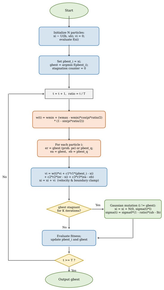
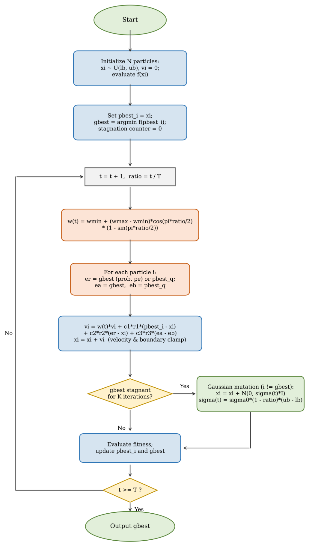
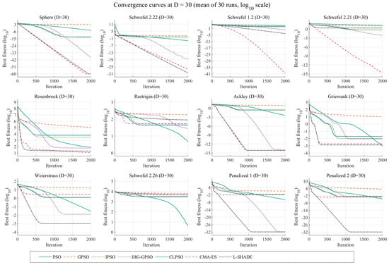
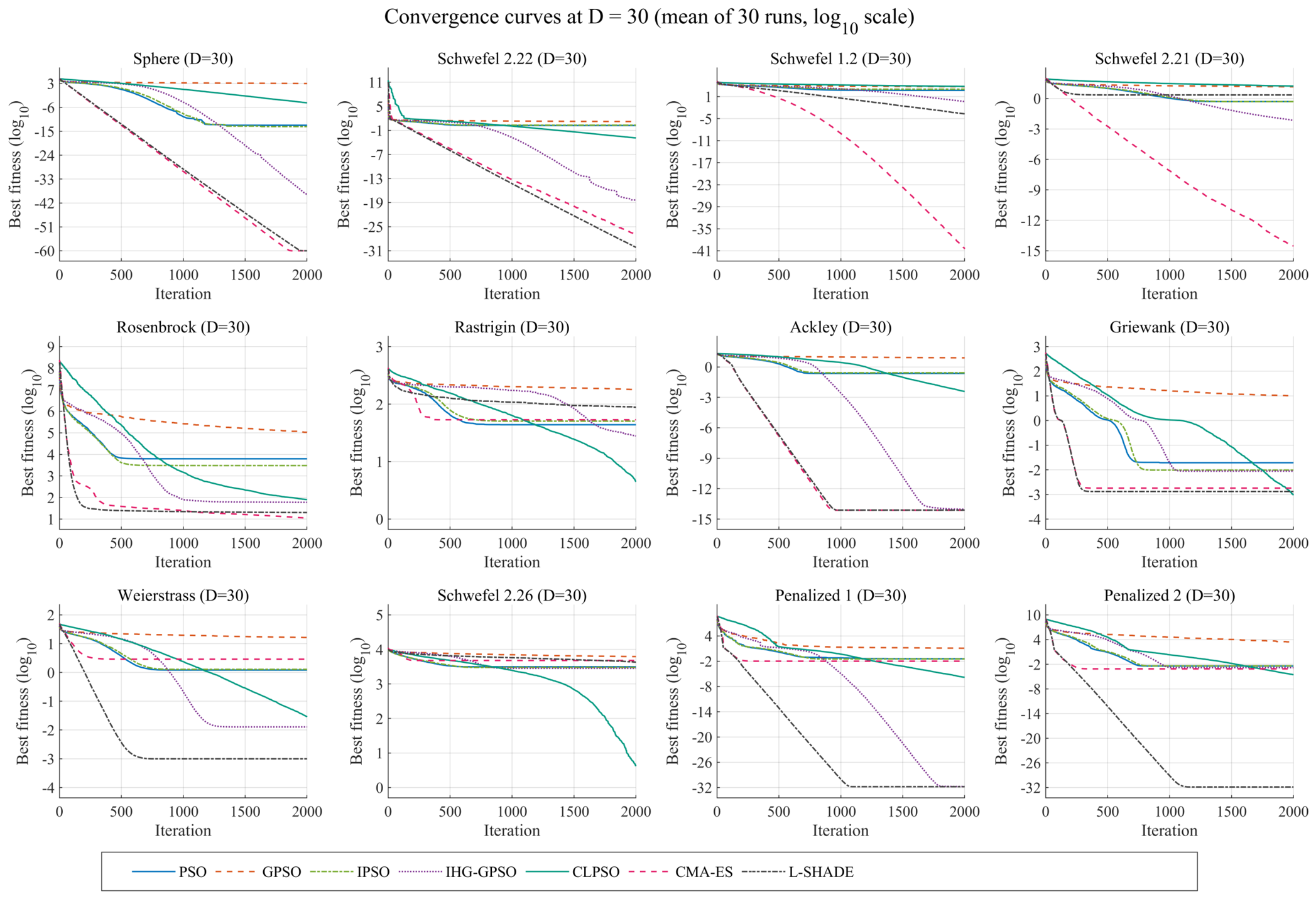
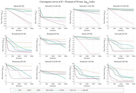
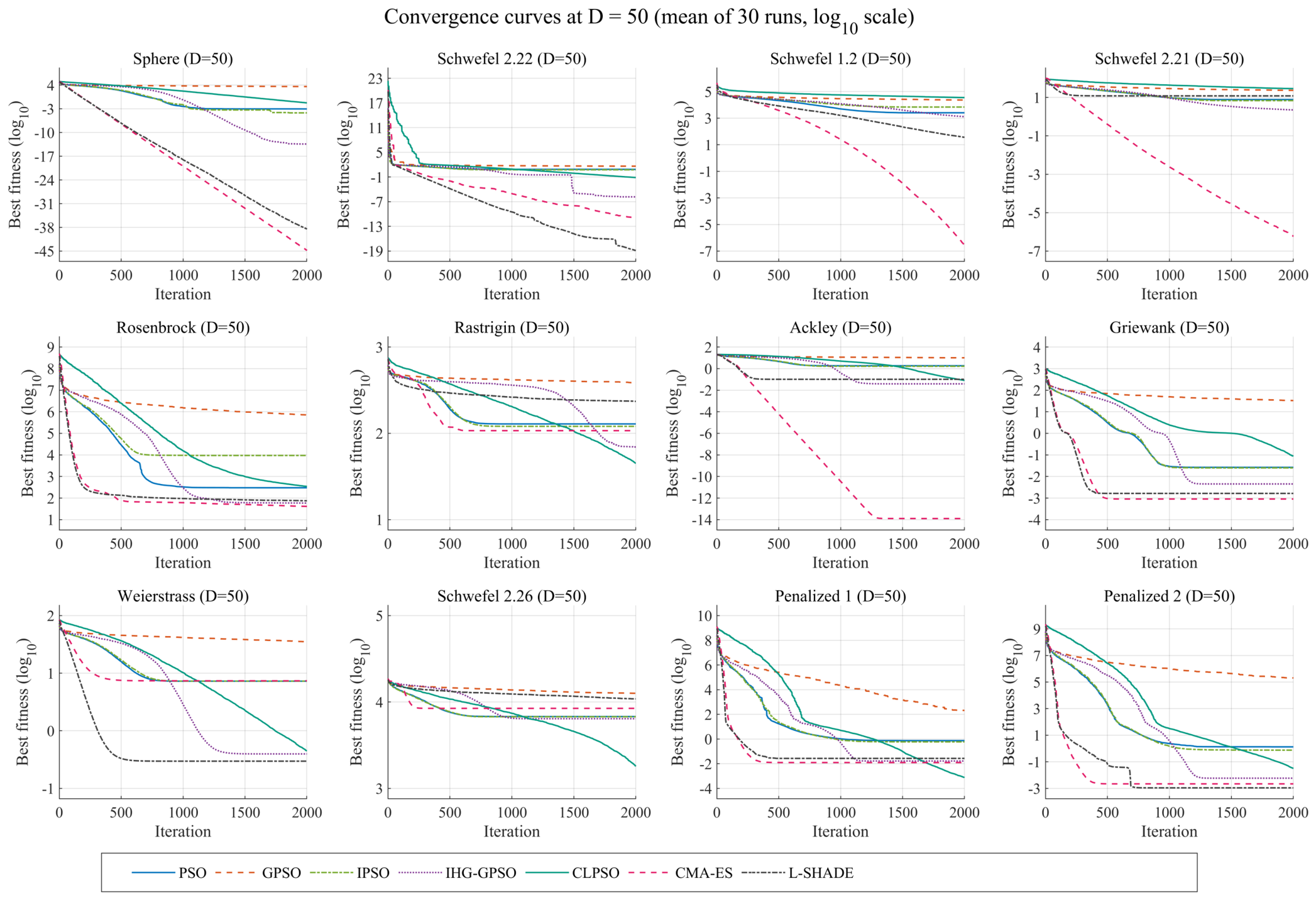
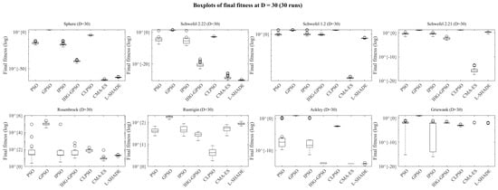

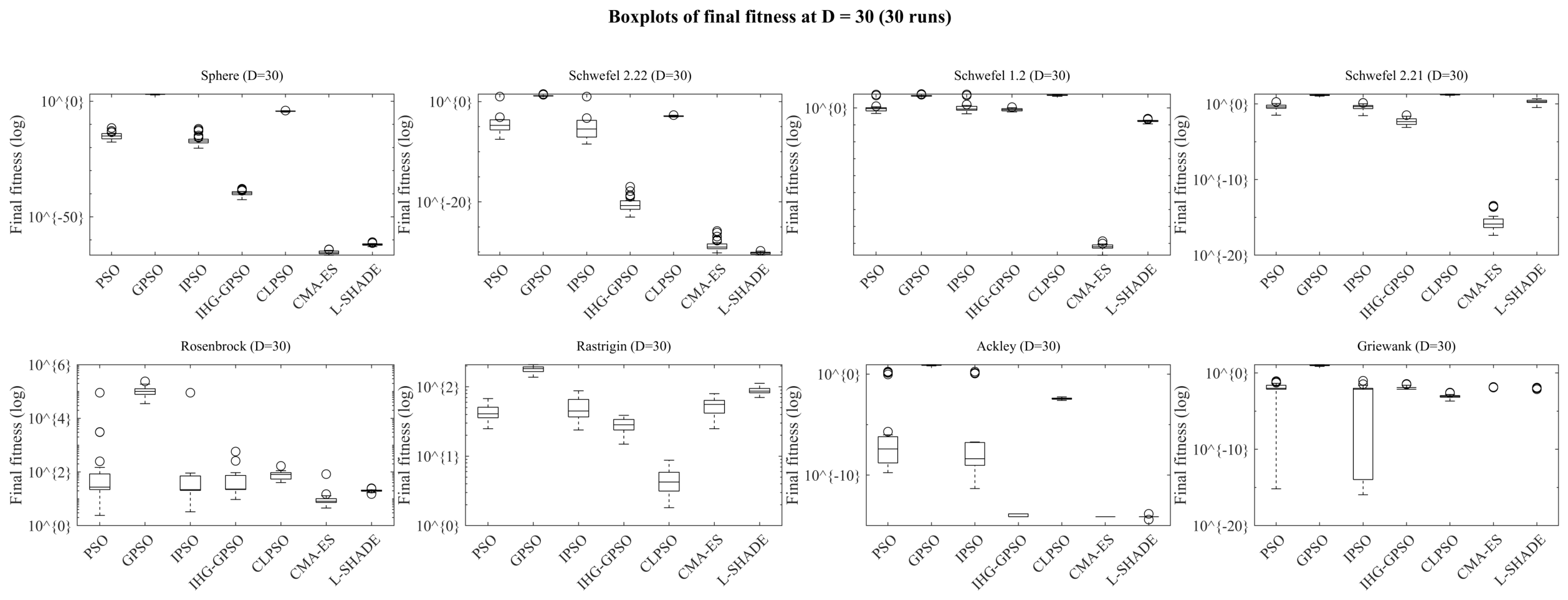

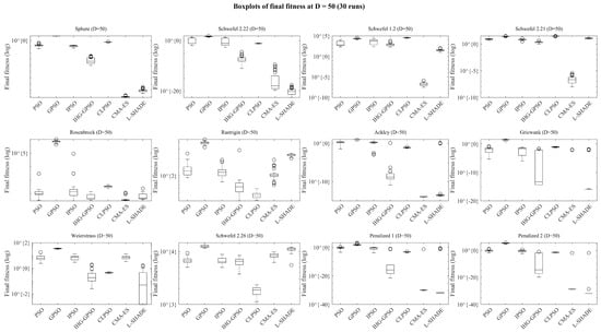
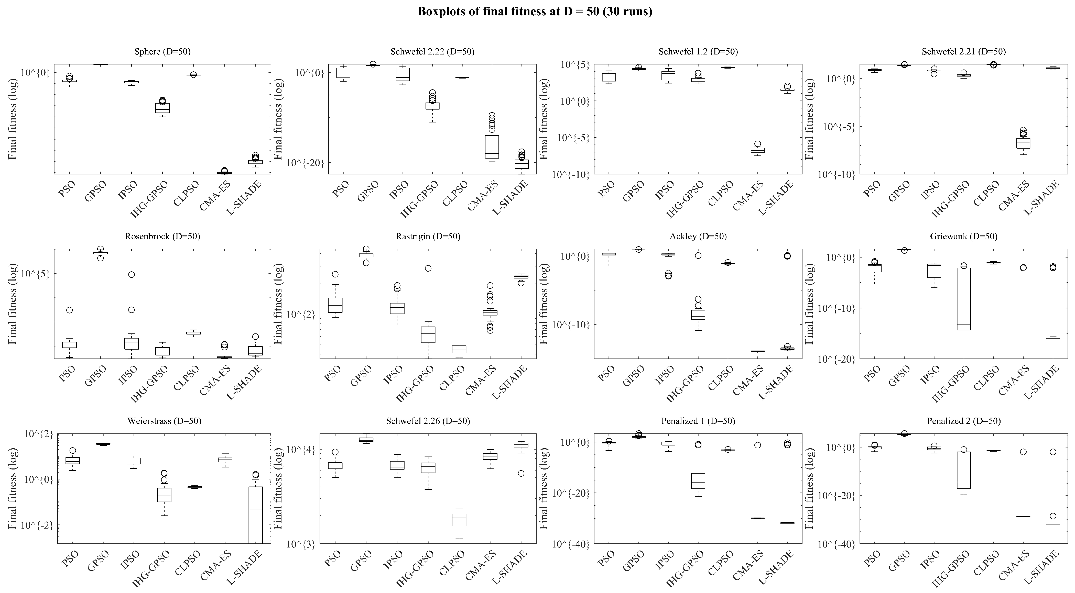
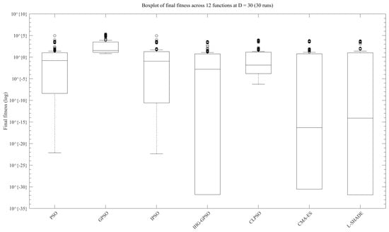
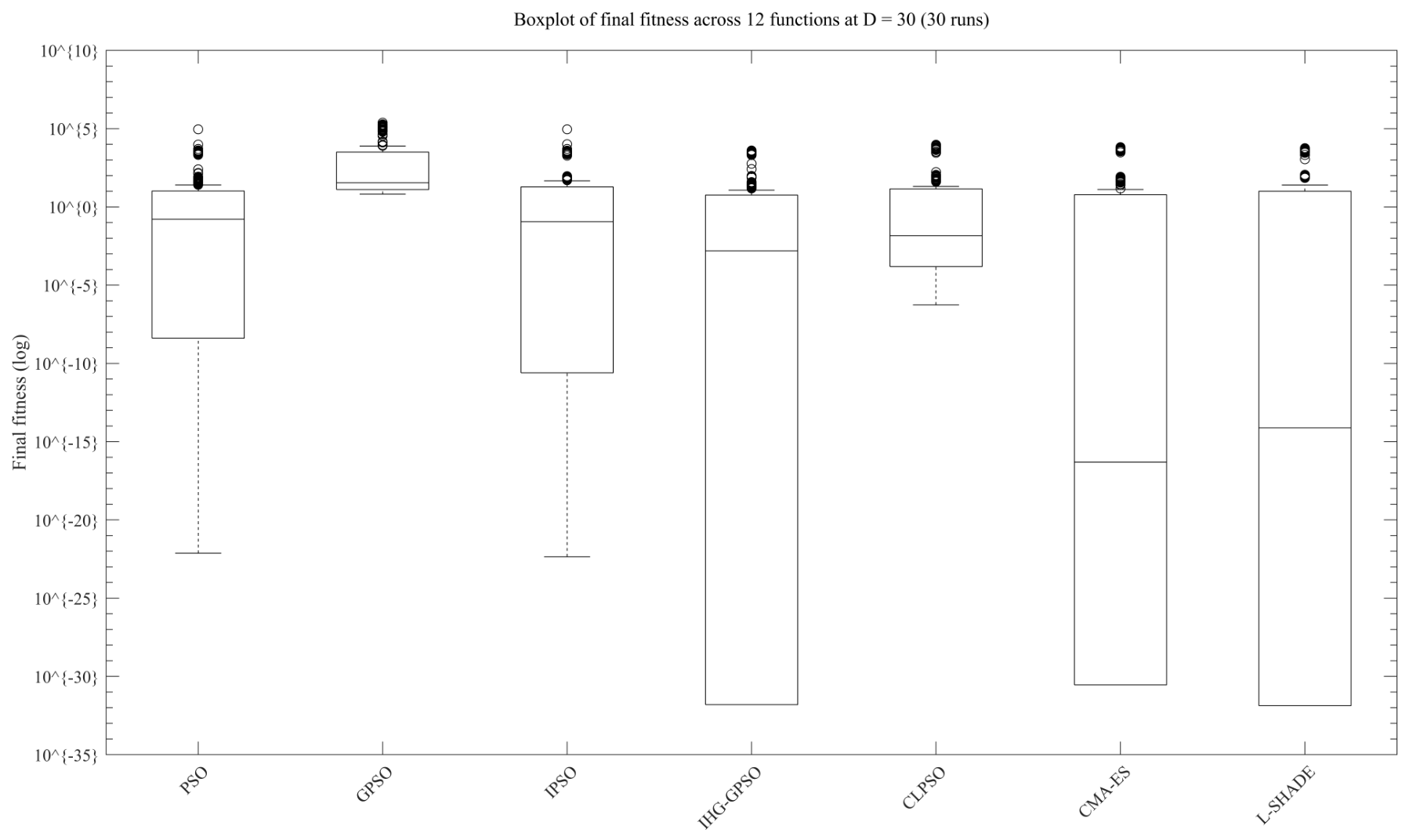
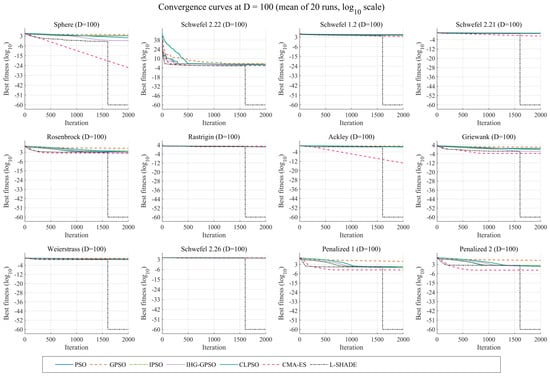
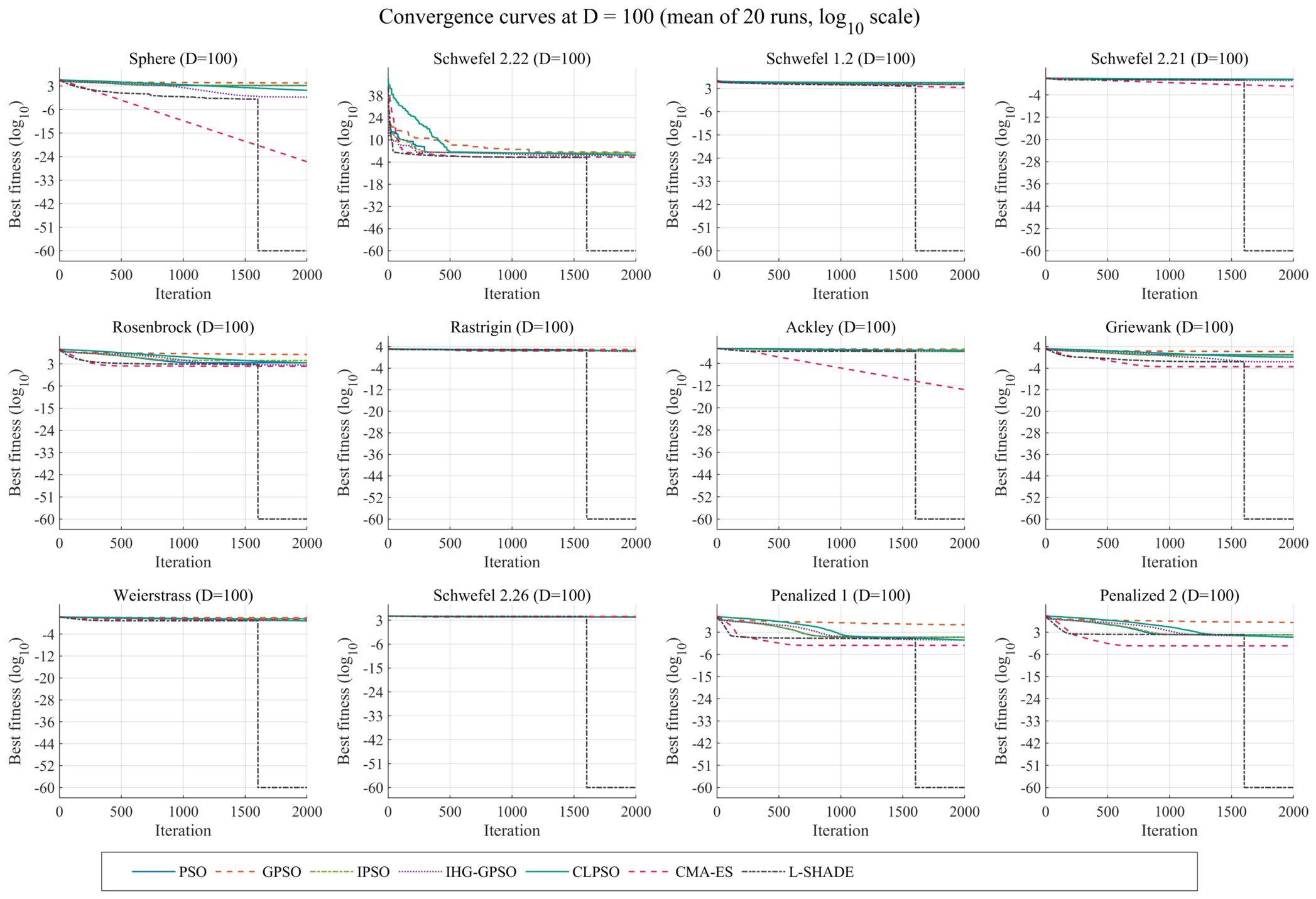
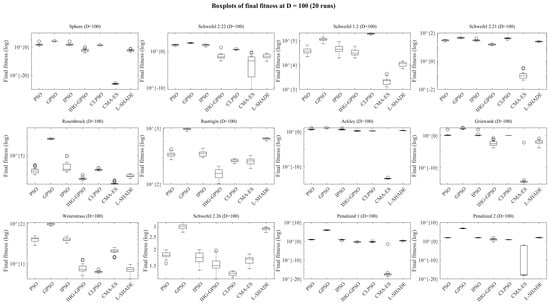
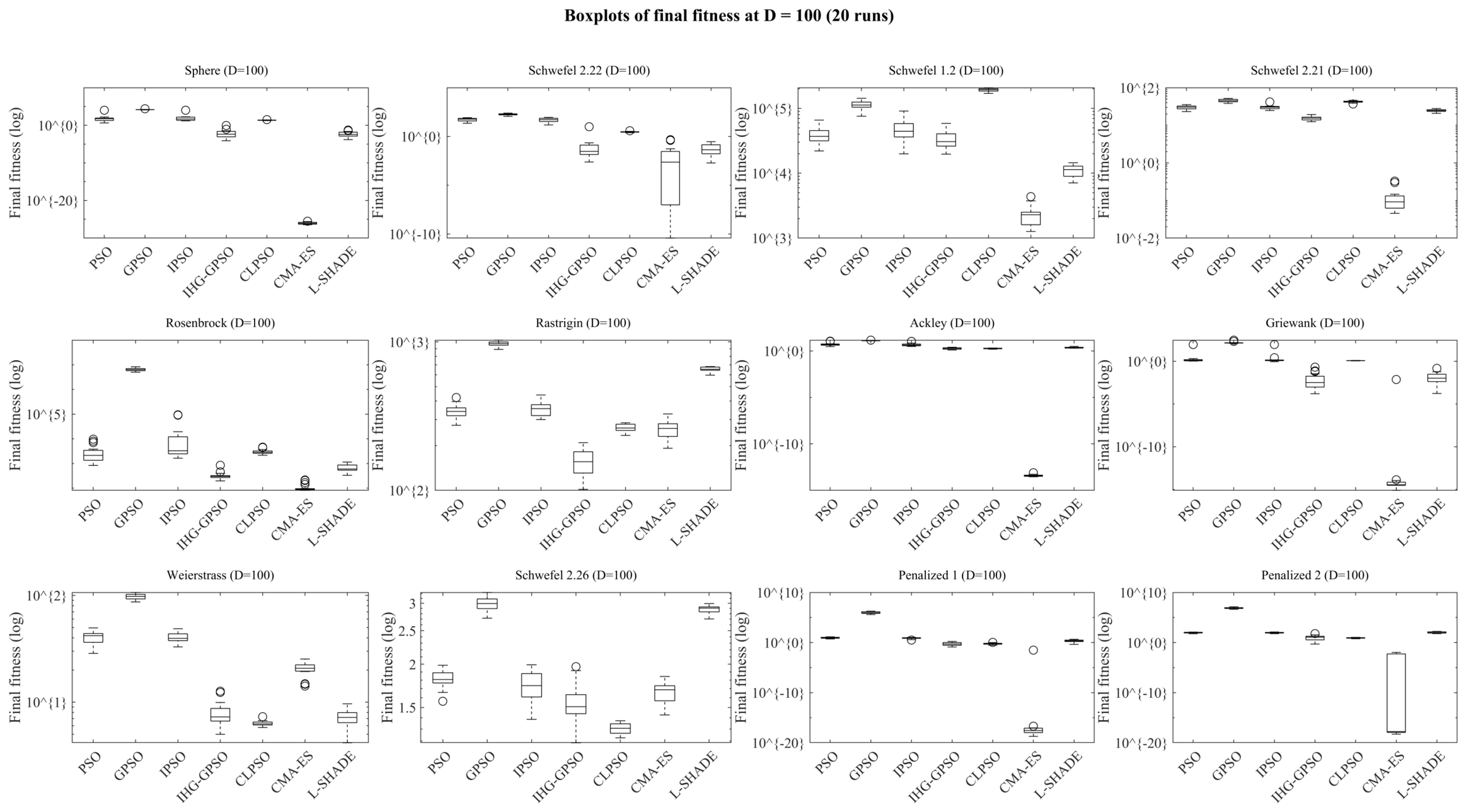
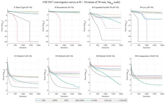
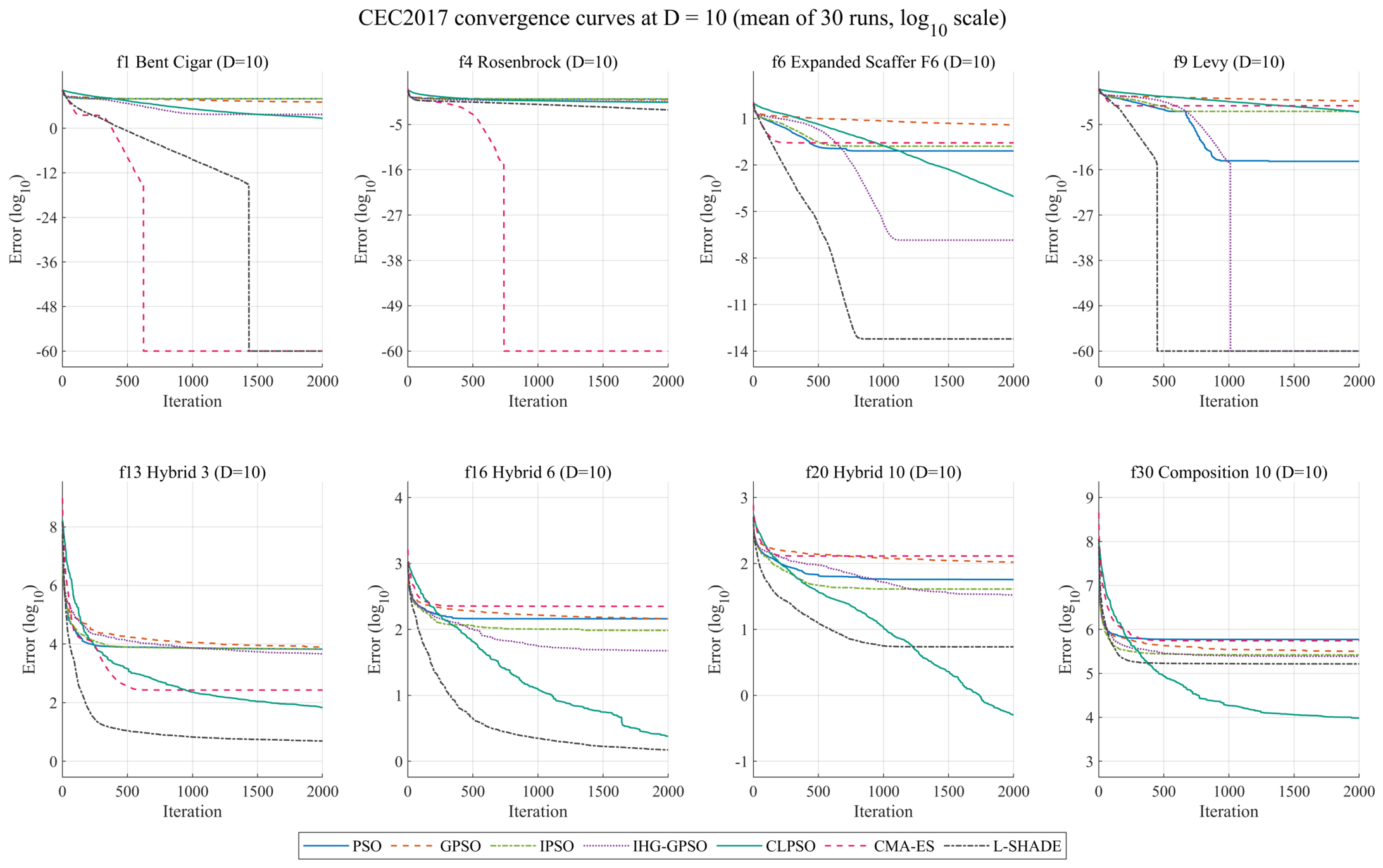
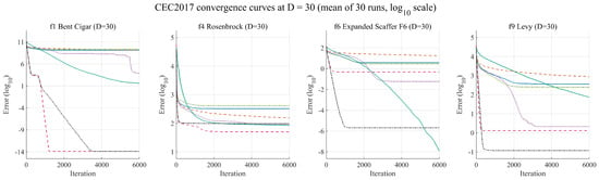
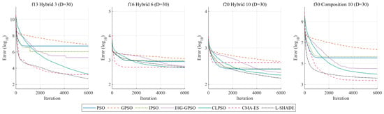
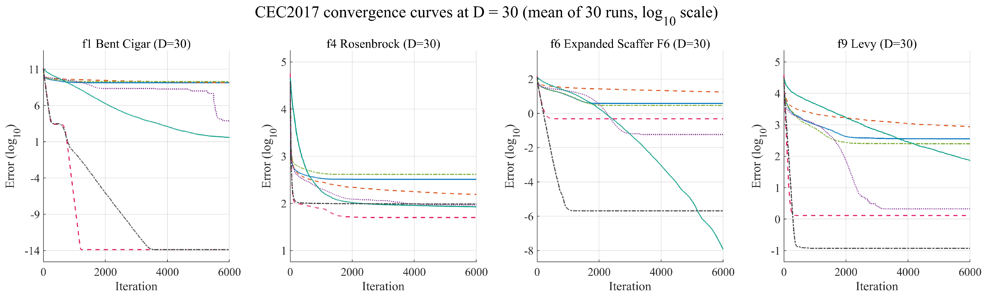
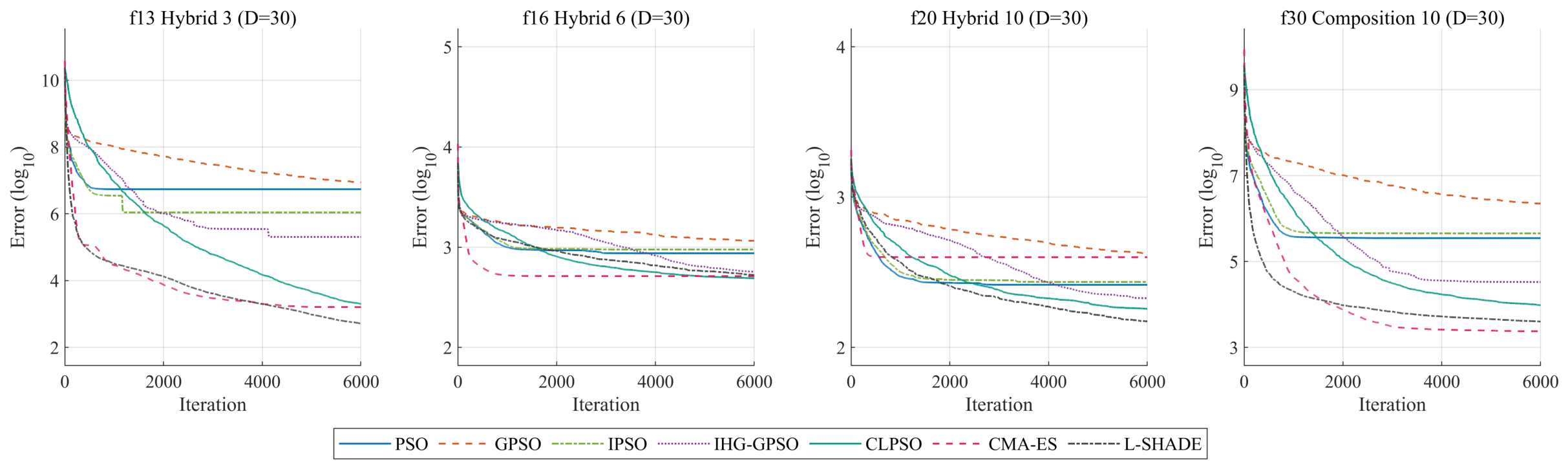
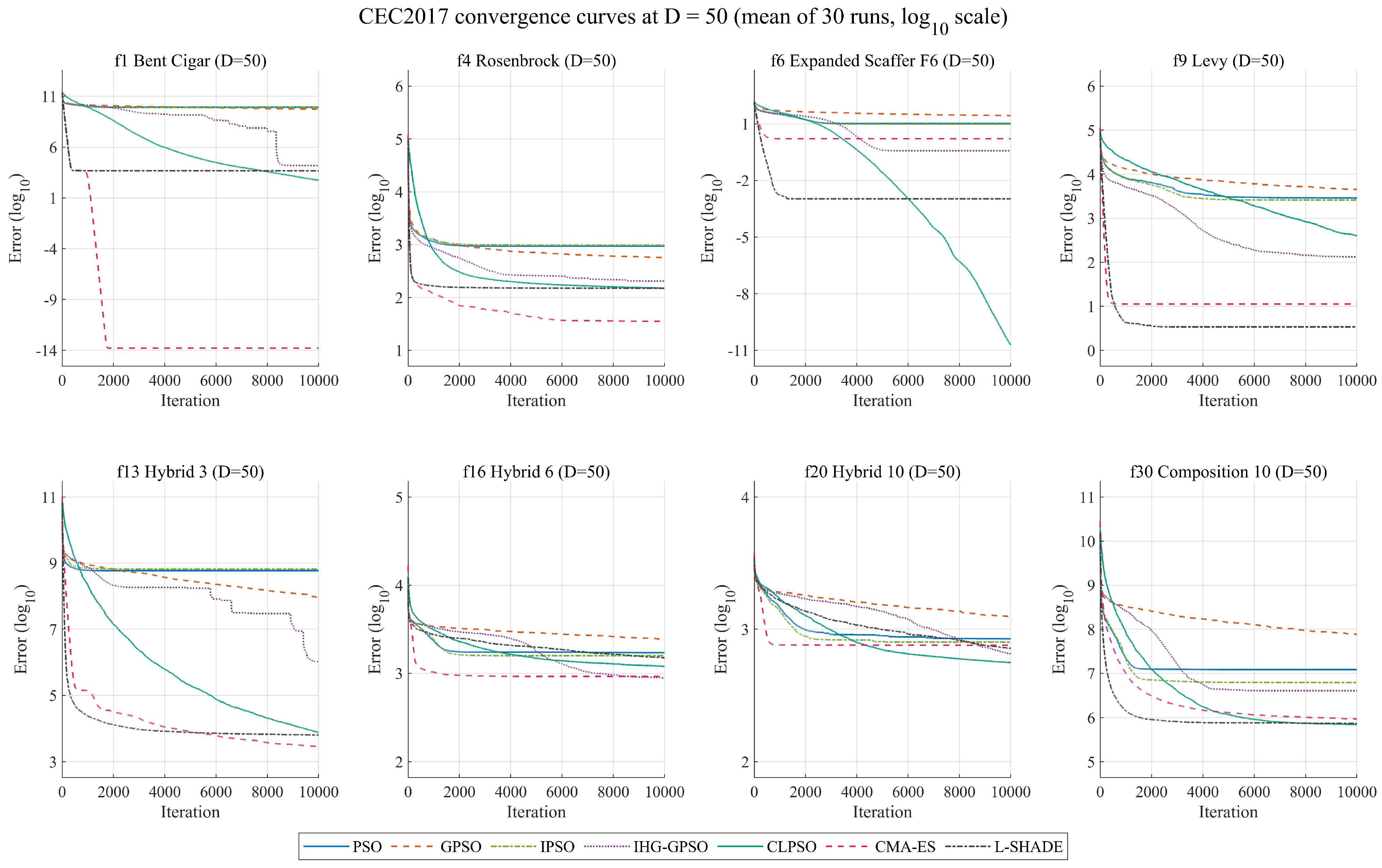
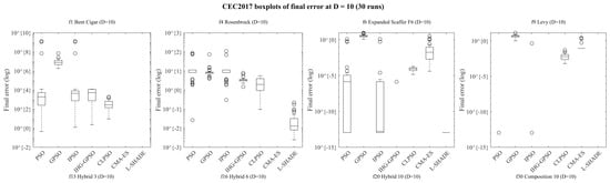
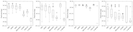
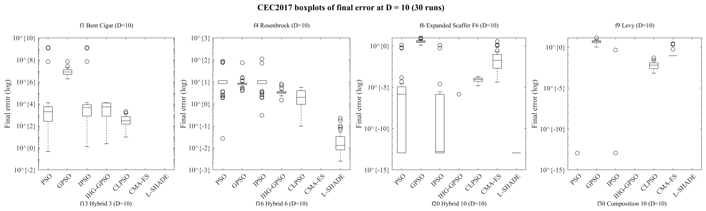
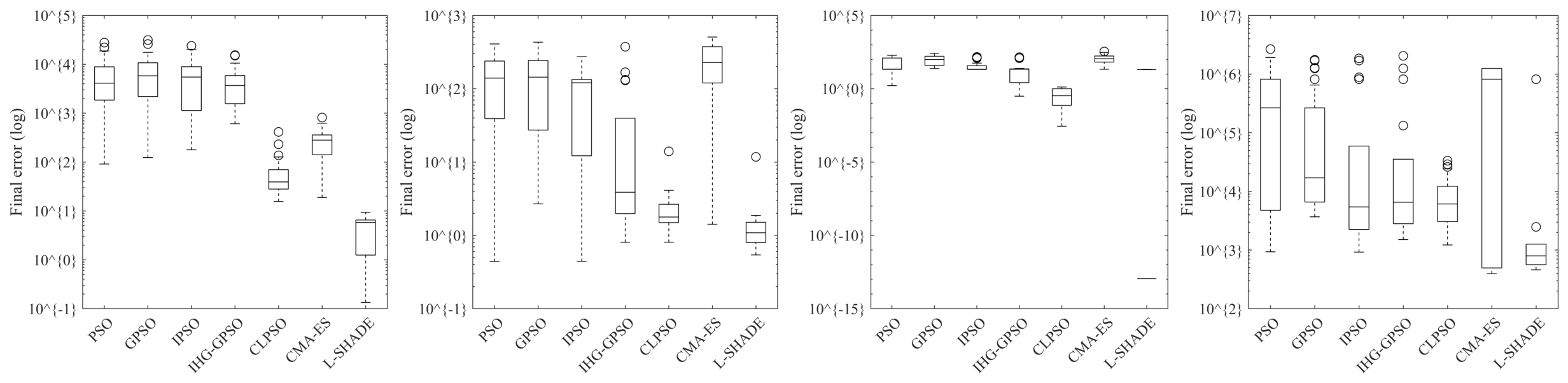
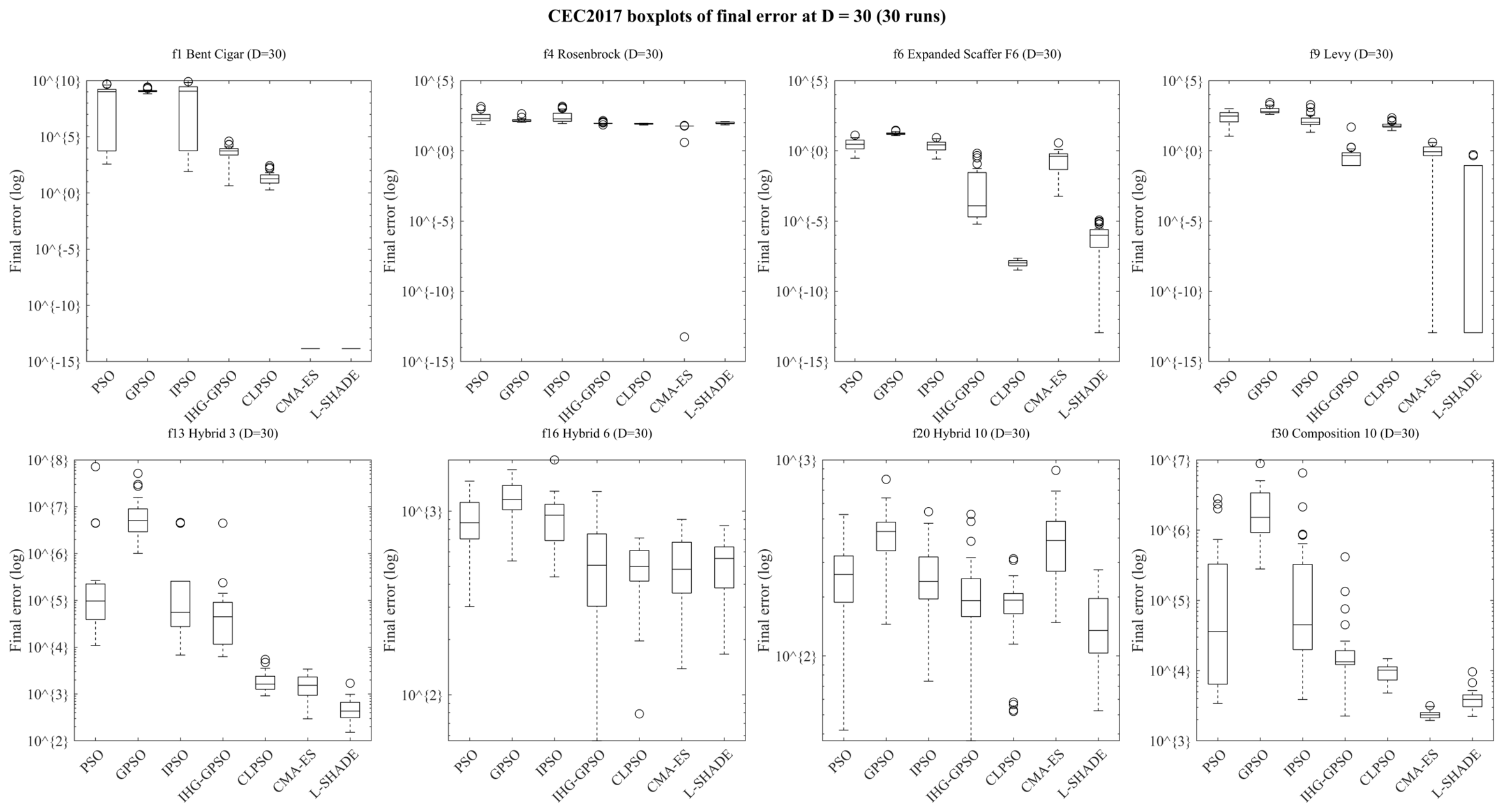
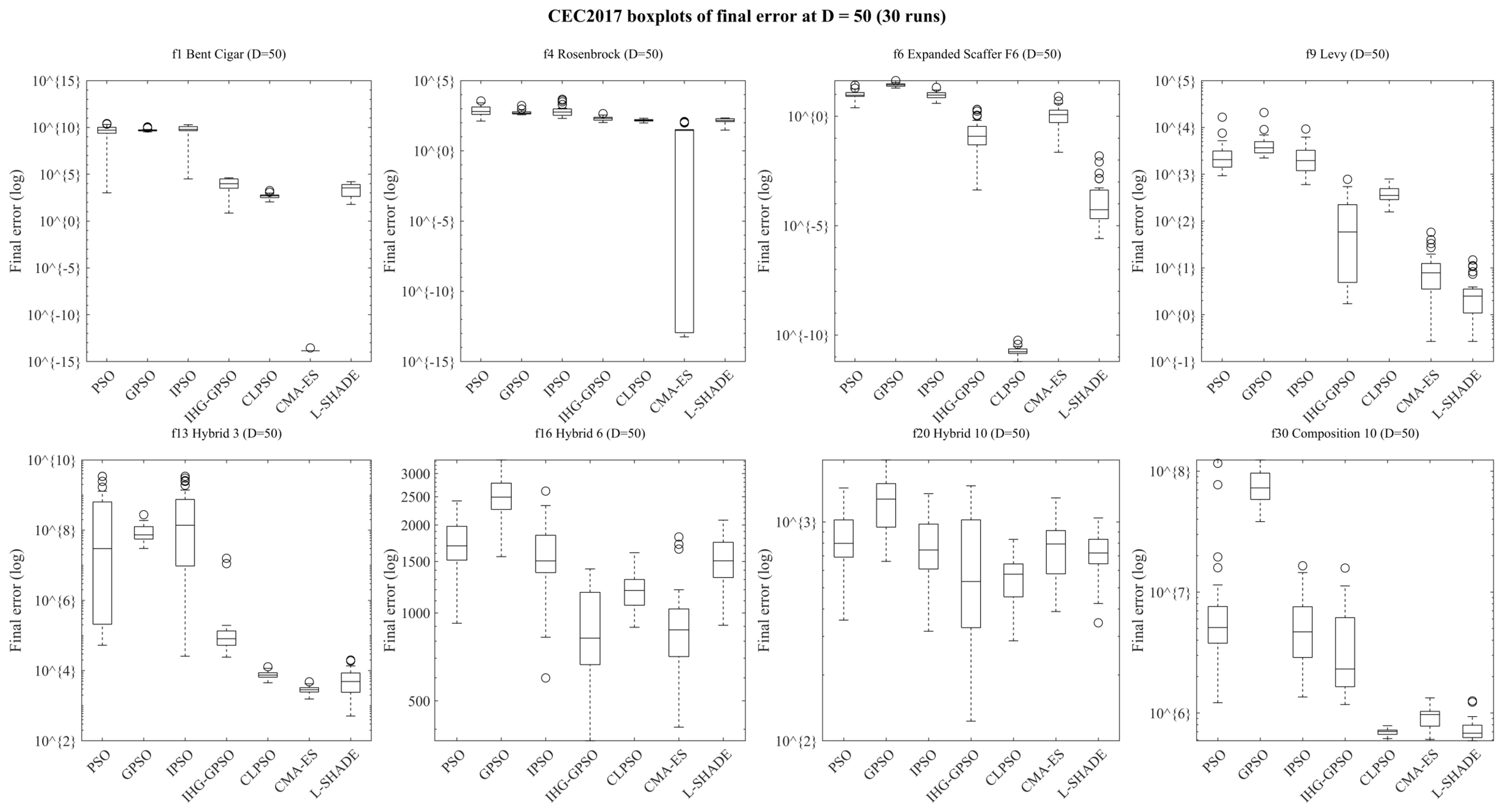
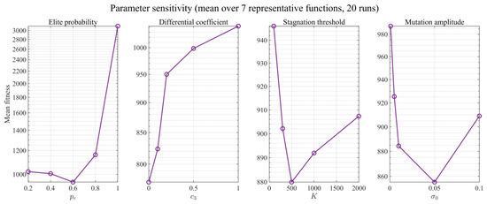
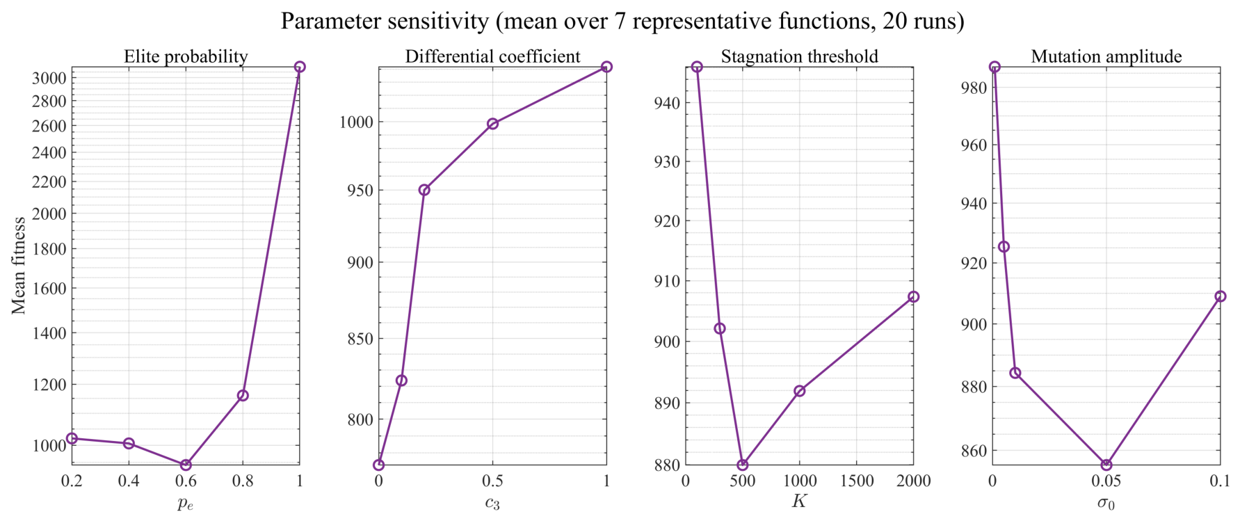
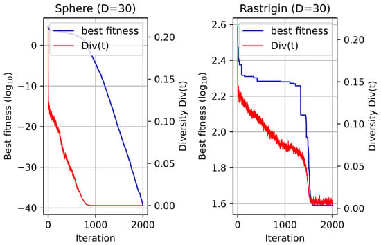
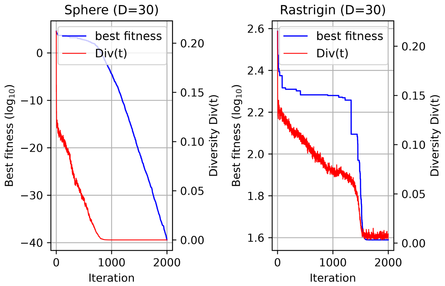
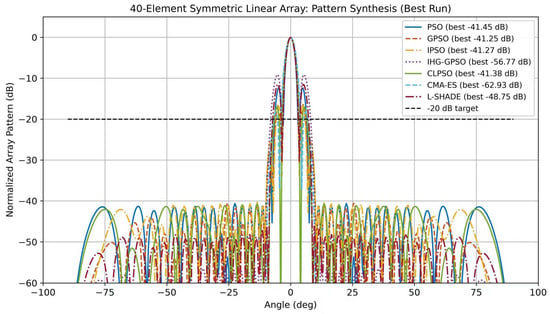
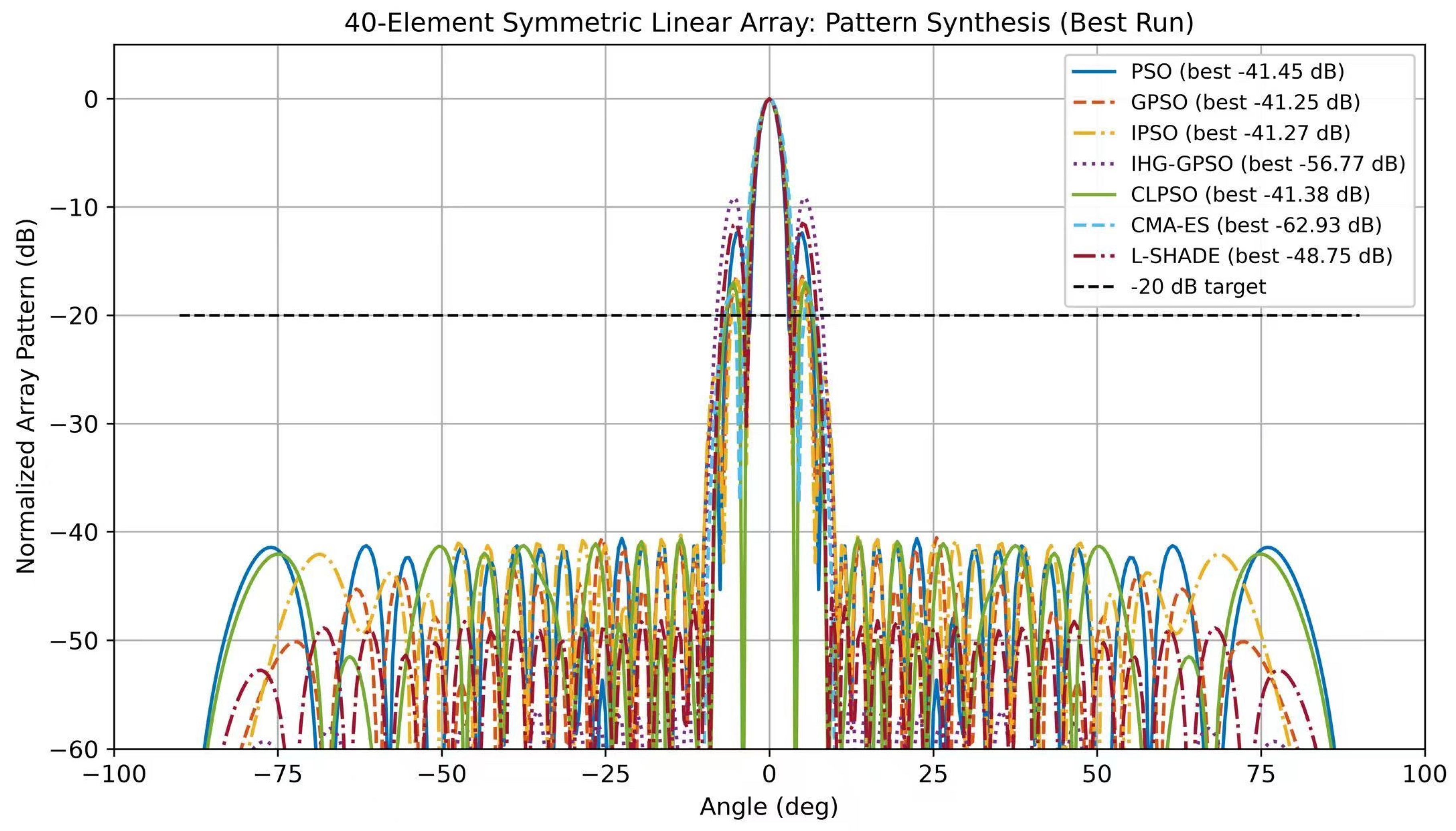

Disclaimer/Publisher’s Note: The statements, opinions and data contained in all publications are solely those of the individual author(s) and contributor(s) and not of MDPI and/or the editor(s). MDPI and/or the editor(s) disclaim responsibility for any injury to people or property resulting from any ideas, methods, instructions or products referred to in the content. |
© 2026 by the authors. Licensee MDPI, Basel, Switzerland. This article is an open access article distributed under the terms and conditions of the Creative Commons Attribution (CC BY) license.