


Abstract
Scarce medical images often prompt data augmentation. We ask when it earns its opportunity cost under a complete information budget. Across four collections, classical and GAN candidates are compared with real-only training, full-pool exposure, score adjustment and direct label use. Transformations reduce within-patient variation; source mismatch and between-patient uncertainty remain. Fixed 50-model ResNet50 ensembles with ranked classical candidates and probability averaging outperform equally adjusted real-only and full-pool ensembles at five sizes. We evaluate procedures in 50 paired draws at 50, 100, 150, 200 and 250 image-training patients. The design counts 200 regularization patients plus disjoint 100-patient selection and adjustment sets. Evaluation includes 38,743 CheXpert patients. At 250 patients, guidance reduces maximum group cross-entropy by 0.0442 versus real-only training (simultaneous 95% interval, 0.0048–0.0836). Adding the 100 selection patients to each original training cohort outperforms using their labels only to guide augmentation at 50–200 patients. Thus, use independent labels first when cohorts are smallest; consider selected augmentation once patient evidence, strong representation and aggregation are available. The 250-patient result marks the upper tested setting, not a universal threshold. AUROC remains stable while sensitivity and specificity shift, requiring operating-point review.
Keywords:
data augmentation; gradient alignment; synthetic data; worst-group loss; medical imaging; data selection; distribution shift MSC:
90C47; 62G35; 68T07; 68U10
1. Introduction
Many practical imaging projects begin with tens or hundreds of image-training patients, and an underrepresented label/projection cell may contain only a handful. The immediate development decision is where the next unit of effort should go: direct use of existing labels, representation learning from unlabeled images and reports, targeted annotation, cross-site collaboration, or transformed views of the same patients [1,2,3,4]. Transformations can encode useful invariances [5,6,7,8], but their value depends on what they improve and what the same resources could achieve. We therefore define augmentation value by an endpoint, a comparator, a complete label budget and an uncertainty target.
We study chest-radiograph opacity classification across RSNA/NIH controlled source experiments, BIMCV [9] external evaluation, CheXpert new-site transfer and a Kermany [10] target-shift screen. Maximum group cross-entropy across the four opacity-label/anteroposterior (AP) or posteroanterior (PA) cells is the primary endpoint. It directly measures the worst predictive loss among the declared cells. Fixed-predictor risk and the expected performance of a newly fitted procedure are evaluated separately. In the five-size experiment, 50–250 patients enter each image-training fit; the complete resource design also counts 200 regularization, 100 selection and 100 score-adjustment patients. Comparator-specific use of these auxiliary labels is reported throughout.
The gradient-guided rule ranks candidates by alignment with the current worst-group gradient and selects their weight using an all-group smoothness bound that includes zero. The bound governs one update; external comparisons evaluate the complete 100-update continuation. A matched-summary example and two variance calculations show why transformations can improve the use of observed patients while source discrepancy and between-patient uncertainty remain.
Successive controls isolate coverage, candidate source, ranking, weighting, output correction, probability aggregation and total label availability. They identify one supported configuration: a strong ResNet50 representation, moderate coverage, ranked classical candidates and probability aggregation. Fixed ensembles in this configuration improve on equally adjusted real-only and full-pool ensembles at every tested size. In the locked new-fit analysis, adding the 100 selection patients to each original training cohort and refitting is superior at 50–200 patients; at 250 patients, that contrast becomes unresolved and guidance improves on real-only training, while the full-pool contrast remains unresolved. The resulting allocation rule is staged: add independent patient information first when cohorts are smallest, then consider selected augmentation to improve the use of a larger fixed cohort.
Score adjustment keeps the image representation and logistic head fixed while changing output logits using guidance patients. The original procedure adds a projection-specific offset; the later search also rescales logits (Section 3.6). Both minimize maximum guidance-group cross-entropy. In the final experiment, candidate selection uses one balanced 100-patient set and adjustment uses a disjoint balanced 100-patient set. The procedure controls for output correction; probability calibration at clinical prevalence is a different objective.
Table 1 maps each dataset and follow-up to its evidence role.
Table 1.
Study sequence and evidence status. RSNA regularization, guidance and check partitions are patient-disjoint from current training cohorts. “Frozen” denotes a documented local decision freeze.
Each successive control in Table 1 resolves a specific alternative explanation. The final size design was informed by the earlier CheXpert results; its protocol, source choices and 18-contrast primary family were then frozen before applying 10,500 heads to CheXpert. The sections that follow connect distributional evidence [11,12,13,14], the tested intervention and the resulting practical decision rule.
2. Theoretical Foundation and Motivation
Candidate-level similarity is insufficient to establish training value. An augmentation source may reproduce opacity-label and AP/PA frequencies while changing the image–label relation needed to recognize opacity. The distinction can be made explicit in a small example. Let denote the binary label and a simplified nuisance feature, such as an acquisition-related attribute. Both are balanced and independent. Let X be the feature used for diagnosis. In the target population, : positive and negative feature values identify the corresponding labels. Candidate source A preserves this relation, whereas source B reverses it, . Table 2 lists every possible label–nuisance pair.
Table 2.
Constructed example: each row has probability in both candidate sources and the target. Label and nuisance summaries agree, while diagnostic information differs. This is an illustration, not an empirical image result.
Both sources have the same four group probabilities and nuisance–label moment . A criterion using only these quantities cannot distinguish them. Their induced prediction directions nevertheless differ. For illustration, consider symmetric logistic rules with magnitude : fitting to A favors , whereas fitting to B favors , where is the logistic function. On the same target population, their mean cross-entropies are
At , these are approximately 0.127 and 2.127. At threshold 0.5, the first rule classifies every target example correctly and the second reverses every label. Identical group summaries can therefore coexist with opposite learning value; richer measures of the joint image–label distribution may distinguish the sources.
Accordingly, the experiments evaluate candidates through their effect on the classifier. The scalar mixture criterion in Supplementary Methods S6 determines how much a source moves a declared moment toward its target; the downstream controls determine whether that source also improves prediction. Related robust reweighting and group-shift work motivates this formulation [15,16,17,18].
2.1. Generated Views Can Improve Use of Existing Information Rather than Patient Information
Let denote the real training patients and let be m generated or transformed images, where G is fixed and the random seed U is independent of the random unknown target-population quantity T in a statistical model and . Conditional on , these images contain no additional information about T:
Here, I denotes mutual information; the statement applies whenever the quantities are well defined. It follows directly because the conditional distribution of depends on and independent randomization, not on T. Thus, increasing m cannot turn the same n patients into additional independent observations of the target population. A generator with external training data or an externally supplied prior is outside this conditional argument: that information must be counted separately. The frozen ImageNet-pretrained representations in our experiments are such shared external resources and are held fixed across arms. They can improve feature quality and reduce task-specific fitting but do not add independent target-patient observations; uncertainty therefore remains when only a few patients populate a label/projection cell.
Candidate generation and guidance selection require different resource accounting. Our selected pool also depends on labels of 200 separate guidance patients; its information is not exhausted by . For that pool, the conditioning set must include all real training, guidance and regularization data and the fixed external representation. Independent randomization adds no information conditional on this complete resource set, but guidance selection can use real information absent from alone. The nominal 144/180-patient image-training budget per member therefore differs from its total 544/580-patient real-label availability. Section 4.7.2 tests controls that use those guidance patients directly for training. This accounting prevents attributing additional real-label information to synthetic images.
Augmentation can still improve a fitted classifier by encoding invariances, changing regularization, or reweighing the empirical objective. It changes how a learner uses observed information rather than the number of independent patients observed. With few patients in a group, candidate quantity and matched group frequencies therefore require a downstream test of learning direction.
2.2. Candidate Quantity Cannot Remove Between-Patient Uncertainty
Candidate quantity and patient count affect different sources of error. A two-level model makes this distinction explicit. At a fixed parameter and with a fixed patientwise transformation rule, let be independent patients from one group and the gradient from their jth independently randomized transformation. Put , , and . With finite second moments,
The three terms are source discrepancy, between-patient variation and within-patient transformation variation. Increasing transformations per patient reduces only the last term. An accurately estimated but unsuitable candidate direction therefore remains unsuitable as , while an undercovered group remains limited by its own patient count. Exact duplicates have and add no variance reduction. Classical transformations assume local label preservation; generated candidates can additionally inherit source mismatch. Our controlled comparisons test both sources by their downstream effect across coverage deficits. Supplementary Methods S2.3 proves the fixed-parameter, fixed-rule decomposition. Data-fitted heads and generators introduce further dependence, for which training-set stability analysis provides a complementary framework [19].
The decomposition also yields a patient-count floor for a declared gradient-error tolerance . Write , and . Even infinitely many transformations leave error . When , a finite transformation count can attain error at most only if and
When this condition holds, the model requires . If , the boundary case can attain the tolerance, but further transformations have no effect. Thus, candidate quantity cannot cross the independent-patient floor of this fixed-rule model. The five-size experiment determines where empirical utility appears rather than imposing a numerical threshold.
3. Materials and Methods
We use one gradient-guided intervention as a worked case for the evidence questions developed above. Its definition makes candidate selection and weight explicit, so matched controls can test their contributions. The rule answers one local question: if augmented images influence the next update, do they move the model toward lower group loss? The initial implementation uses a frozen ImageNet-pretrained ResNet50 representation and a regularized logistic head shared across candidate sources and controls. AP/PA projection and the binary opacity label define four evaluation groups. We report maximum group cross-entropy, the largest mean prediction loss among these groups; lower values are better. The empirical comparisons then ask whether the resulting continuation still adds value against matched exposure, equally adjusted real-only training and training-randomization uncertainty. The mathematics below separates these claims before the results are considered. Table 3 summarizes the five experimental stages.
3.1. Local Admissibility of an Augmentation Step
Let be the mean cross-entropy on guidance patients in group g. Suppose a real-data step has produced parameters and consider an additional displacement induced by augmentation. For a smooth group loss,
The sign determines the local effect. If , the augmentation direction is locally favorable for group g; if it is negative, the first-order change increases that loss. Candidate utility is therefore tied to the training direction, not to the number or visual plausibility of candidate images.
A first-order calculation is not enough to choose an arbitrarily large augmentation weight. If has -Lipschitz gradient, smoothness gives
The linear term favors a beneficial direction; the quadratic term limits the size of the intervention. For the maximum group objective, this yields
For fixed d, is the maximum of convex quadratics and is convex on . We evaluate the grid ; including zero permits no augmentation. This property of weight selection does not establish optimality of candidate ranking. There is nevertheless an exact empirical safeguard: if minimizes the valid bound over a grid containing zero, then
This guarantee compares one augmented step with its matched real step on the guidance loss. It does not extend automatically to the fixed 100-update continuation or to a new population.
3.2. Conditions for Strict Local Improvement
Let , and . For a nonzero candidate displacement d and positive , Equation (5) certifies a strict reduction relative to the matched real step whenever, for every group,
For each currently worst group, : its alignment must be positive and the step small enough that the linear improvement exceeds the curvature term. Groups with smaller initial loss have positive slack; they can tolerate a limited increase without becoming the new worst group. Requiring positive alignment for only one group is therefore insufficient, especially at a tie.
More exactly, for the active set , the directional derivative of the finite maximum is
It is strictly negative precisely when every active group has . For the convex logistic group losses used here, if any active group has , convexity gives for all . No positive step along that fixed direction can then strictly improve the empirical maximum. If , the augmented and real one-step updates coincide exactly. These are mathematical explanations of how candidates can fail to add value even when their number is large. Failure of the sufficient smoothness certificate alone, however, is not proof of failure: the bound can be conservative.
The conditions concern observed guidance losses, a fixed representation and one update. They do not guarantee population benefit, certify preservation of diagnostic structures, or prove improvement after 100 updates. Scarce training coverage and uncertainty in guidance gradients remain constraints. The experiments test whether the complete continuation realizes a benefit and whether that benefit exceeds simpler interventions.
3.3. From a Fixed-Predictor Comparison to a Population Certificate
Local admissibility and external utility are different claims. For a finite family of predictors frozen independently of new evaluation patients, simultaneous confidence bounds can compare population maximum group risks while allowing the maximizing group to change. Let bound each predictor’s group risk, and let bound the paired group loss difference. A valid upper bound on , where , is
A negative right-hand side certifies a population gain under the sampling assumptions; a nonnegative bound establishes neither benefit nor absence. The result follows because for every baseline group h. Supplementary Methods S2.4 constructs simultaneous empirical-Bernstein bounds [20] from analytic loss ranges, with one overall error probability. Unlike a bootstrap approximation, these bounds provide a finite-sample guarantee for independent within-group patients from the selected label-defined population.
The uncertainty is governed by the number of independent patients in each evaluation cell, rather than the number of synthetic training images. Supplementary Methods S2.4 also gives a simple sample-size condition showing this dependence. We report the conservative certificate separately from the primary paired-bootstrap analysis. In particular, an empirical local guarantee, a patient-conditional ensemble contrast and a guarantee for a newly randomized training procedure must not be treated as interchangeable.
3.4. From Individual Candidates to the Evaluated Direction
For image features x and binary label y, let be the logistic prediction and . Let be the fitted reference parameters, the balanced real-data loss gradient at and the corresponding gradient of a retained augmentation pool. With learning rate and quadratic-penalty coefficient , the real and mixed updates are
where . The shared quadratic penalty cancels from the augmentation-versus-real displacement; the endpoint remains unpenalized cross-entropy.
Candidate ranking uses the group that currently has the largest guidance loss. Let and let be the data-loss gradient of candidate i. We score
A larger score indicates that, relative to the real-data gradient, the candidate points more strongly toward a local reduction in the current worst-group loss. We retain the declared top fraction within each label/projection cell, recompute the balanced pool gradient , and then choose by minimizing Equation (5) across all groups. Ranking therefore focuses the pool on the current deficit, while weight selection evaluates the maximum across all groups.
Real and candidate gradients are evaluated at ; guidance gradients are evaluated at . The bound applies to the resulting fixed displacement from . Ranking retains a heuristic top fraction and, at ties, uses one declared maximizing group; the bound evaluates all groups. We then hold the selected pool and weight fixed for 100 updates. Supplementary Methods S2 gives the derivation; local training influence has established precedents and limitations [21,22].
3.4.1. Worked Example
Take one group with , , and . Equation (4) gives changes of at and at . Positive alignment favors augmentation, while curvature limits the admissible weight. If the alignment is , both bounds are positive and zero is preferred. These numbers illustrate the decision rule rather than report fitted measurements.
3.4.2. Operational Workflow
Table 4 states the complete procedure. If no retained pool improves the local maximum-group bound, the decision is to keep the real update rather than force augmentation.
Table 4.
The tested group-loss-guided intervention. All selection quantities are computed before the final continuation is evaluated; its local decision and independently evaluated utility are separate claims.
3.5. Patient Roles and Controls in the Development Design
The original paired regimes compare balanced coverage with a shortage in one label/projection cell, but their total counts also differ. Section 4.6 adds a comparison at fixed total count. The classical and GAN arms test two ways of forming candidates from the same training patients; the additional-real arm tests an intervention that actually increases the patient-information budget. Matching heads and continuation updates limits optimization differences, while the later pool controls address exposure and selection.
Three balanced cohorts contain 180 patients each, with 45 per label/projection cell. Reducing opacity/AP coverage to nine gives a deficient cohort of 144 patients. Its three generative adversarial network (GAN) generators [23,24,25] and six auditors are retrained on the reduced cohorts; the balanced condition uses its matching generators. The previously used RSNA patient bank [26,27] supplies patient-disjoint partitions for regularization (, 200), guidance (, 200) and checking fixed development choices (, 400), all separate from current training and additional-real reserves. Table 1 distinguishes these roles from later external validation and exploratory reuse.
Each initial head receives 400 full-batch updates; regularization is selected from on . Continuations receive 100 updates. A documented pre-fit amendment set the step to , replacing a draft to satisfy a conservative smoothness condition. GAN pools retain 80 images per cell by random, auditor-gated or gradient-guided selection. Classical pools contain four seeded transformations per real image: reflection-padded translations up to 10 pixels, intensity multipliers in and Gaussian noise with standard deviation on the normalized scale, followed by clipping. Guidance retains 25% per cell, approximately one candidate per source image in aggregate. Each cell contributes one quarter of the training gradient.
Fixed classical, random-GAN and gated-GAN comparators use . Ordinary validation also considers random/gated GAN weights and real-only continuation. An information control adds 180 real training patients per replicate; it has a larger patient budget. Equal update counts do not equalize image exposure or total compute. The initial study fits 84 logistic heads. Patient unions across the three cohorts are 512 (balanced) and 409 (deficient), or 989 and 886 with additional real patients. Sensitivity to retention and optimization choices is examined in Section 4.5.
Primary check risk is maximum group cross-entropy. Formal secondary metric definitions are provided in Supplementary Methods S2.6. A paired, group-stratified patient bootstrap with 5000 resamples and seed 20260926 covers 12 declared contrasts jointly and approximately, conditional on fitted models. Cross-entropy is the endpoint of this training protocol; the earlier prediction-mixture protocol retains its Brier endpoint. For the original comparisons, all model weights, input selections and fractions are frozen before their check predictions; later controls have the post-check status specified in Table 1.
3.6. Post Hoc Score Adjustment
Score adjustment changes predictions after training, without changing the image representation or logistic-head parameters. Write for the original logit of replicate j, for projection and . The original offset-only control predicts
A global control shares one offset across projections; the projection-specific control fits one for AP and one for PA. For each fixed real head, the offsets target
The four groups combine label and projection, but the prediction transformation uses only projection, which is available at inference. It never uses the unknown test label to select an offset. The three adjusted replicate probabilities are averaged for ensemble evaluation. For the deficient heads carried into the original external comparison, the stored PA/AP offset pairs are (0.2944, 0.2440), (0.1605, 0.1246) and (0.2466, 0.0125), respectively (rounded here; full precision is retained in the Supplementary Parameter File). Applying these fixed offsets and averaging the resulting probabilities reproduces the specified comparator. The control was added after the initial development check was known; offsets were fitted on guidance patients and then frozen before the additional BIMCV evaluation. No offsets were fitted on BIMCV patients.
An offset changes the model’s confidence and threshold decisions. For example, an illustrative logit gives ; adding gives . At probability threshold 0.5, the adjusted decision is positive when . A positive offset thus lowers the original-logit threshold. Within one projection, it preserves score ordering; different projection offsets can change ordering across projections. The intervention can consequently improve group loss without supplying new patient information.
The later exploratory search extends Equation (9) to , including identity, a shared global pair and separate projection pairs. Slopes lie in and offsets in . Fitting adds a quadratic penalty toward to the maximum guidance-group loss. Two group-stratified guidance folds select the form and penalty from using pooled held-out group loss, followed by refitting on all guidance patients. Both real and guided arms receive the same folds and search budget. Supplementary Methods S7 specifies the optimizer and failure handling. This broader search is distinct from the original offset-only comparator: its results do not replace the originally frozen external comparison. In both procedures, the objective is group-risk balancing; population probability calibration is not evaluated.
3.7. Locked Small-Data Scaling Design
The locked size experiment focuses on classical transformations, which received stronger empirical support than the tested GAN candidates in the preceding analyses. It examines the selected intervention across patient counts rather than comparing augmentation sources again. The final follow-up directly varies the number of image-training patients per newly fitted model: . Fifty paired randomized draws use independently seeded shuffled patient lists within each group, and each smaller cohort is a prefix of its larger counterpart. Draws may overlap because they sample from the same finite source bank. Within every draw and size, balanced, moderate and severe compositions allocate approximately , and of patients to the deficient opacity/AP cell. For example, that cell contains 12–13, 6 and 3 patients at , and 62–63, 31 and 13 at , respectively. Both frozen representations and all declared outcomes are retained.
The 200 guidance patients are split deterministically within group into 100 selection patients and 100 adjustment patients. Candidate ranking and weight selection use only the first half; every reported score adjustment uses only the second. This removes the in-sample adjustment weakness of the earlier information-budget audit. Seven paired arms comprise real continuation, the full fixed-weight transformation pool, a random count-matched quarter-pool, a ranked fixed-weight quarter-pool, the ranked bound-weighted pool and two real-label controls. The direct-guidance control uses the 100 selection patients as the continuation pool with weight 0.2. The stronger add-to-training refit combines the original n-patient cohort with those same 100 patients, reselects regularization on the separate 200-patient partition and refits from zero. This last arm is the equal-label comparator: guidance uses the 100 labels only to rank candidates and select their weight, whereas the comparator uses the same labels to fit the classifier.
The primary estimand is the expected maximum-group CheXpert cross-entropy of an individual newly trained procedure, distinct from the risk of an averaged probability ensemble. The 18-contrast primary family uses adjusted ResNet50 models under moderate coverage: at every size, ranked bound selection is compared with real continuation, the full pool and the add-to-training refit; three additional contrasts compare the mean effects at 50/100 patients with those at 200/250. Five thousand paired two-way bootstrap samples resample both the 50 training draws and CheXpert patients within group. A single maximum-centered-deviation critical value covers the family. The design and code were frozen before all size-curve predictions.
4. Results
The experiments answer three nested resource questions. First, can selected augmentation improve a fixed predictor after equal score adjustment and candidate exposure? Second, does the gain persist when the complete procedure is fitted to a new cohort? Third, if additional patient labels are already available, should they guide augmentation or enter training directly? Table 5 gives the answer before the detailed evidence sequence. Complete secondary results and implementation details appear in the Supplementary Methods and Results.
Table 5.
Resource-allocation summary. CE denotes maximum group cross-entropy; intervals are simultaneous within their declared families.
Figure 1 provides a descriptive view of the candidate sources produced by the declared pipelines. Hash-based example selection did not use classifier predictions or apparent diagnostic severity. The panel therefore documents source output; predictive value is determined by the patient-separated comparisons that follow.
Figure 1.
Representative candidate sources across the four opacity-label/projection cells. Each column shows a held-out real radiograph, a replay of one declared classical transformation on that image and an independently selected accepted GAN sample for the same condition. Examples were selected by SHA256 ordering after model evaluation. The display is descriptive and does not constitute radiological adjudication of anatomical or diagnostic fidelity.
4.1. Initial Gains and Comparator Strength
In the deficient condition, guided classical augmentation selected in all three replicates. Ensemble maximum group cross-entropy fell from 0.7182 for the real reference and 0.7044 for fixed classical augmentation to 0.6628. The corresponding simultaneous differences were with interval and with interval . All three individual guided-classical heads also improved on their matched real references. Maximum group classification error decreased from 0.49 to 0.42; area under the receiver operating characteristic curve (AUROC) changed from 0.7135 to 0.7110. The improvement is concentrated in group-loss balance; ranking discrimination remains similar. Some initially better groups lose performance, as permitted by the maximum-group-loss objective. No declared guided-GAN contrast had a simultaneous interval excluding zero. The balanced condition also showed no established advantage in this original family. Additional real patients improved the deficient ensemble numerically, but their interval included zero. Every stored empirical guidance Taylor bound held numerically. Section 4.5 reports the separated-scoring diagnostics across continuation horizons.
4.1.1. Separating Selection from Augmentation Weight
The fixed classical comparator used a different fraction, so the initial positive contrast did not isolate selection. After seeing the check results, we added 36 further head fits for explicitly post-check controls: the full classical pool at the frozen guided fraction, a random quarter-pool at that fraction and ordinary validation among real/full/random classical alternatives. In the deficit condition, guided classical augmentation retained lower maximum group cross-entropy by 0.0313, 0.0320 and 0.0296, respectively; separate six-contrast simultaneous intervals were , and . These development diagnostics motivated carrying all three comparator heads unchanged into the later locked external-source evaluation.
4.1.2. Score Adjustment Sets the Stronger Reference
The offset-only control in Section 3.6 was added after the initial check analysis and fitted on guidance patients. Projection-specific offsets achieved check risks 0.6492 (balanced) and 0.6420 (deficient), versus 0.7035 and 0.6628 for guided classical selection. Guided minus projection-offset real was in the deficient condition and in the balanced condition. Score adjustment is therefore the stronger development comparator. The projection-offset comparator and the expanded eight-contrast family were carried forward, and all heads, offsets and selections were frozen before BIMCV evaluation.
4.2. Retrospective External Validation Against Score-Adjusted Real Models
We froze the three deficient-condition heads per arm, including the added matched-pool controls and fitted AP/PA offsets, before selecting and retrieving 400 additional adult BIMCV patients. Each cell contains 100 patients; all are disjoint from the previous 800 BIMCV patients. The local protocol specified six simultaneous comparisons: guided classical augmentation against five controls, and offset-adjusted real against unadjusted real. Technical quality control (QC) preceded inference and used deterministic replacements without model outcomes. Eleven images were replaced; an overlap audit against 4202 references found no exact normalized duplicates. The 20 nearest pairs showed no obvious duplicate on technical inspection. Supplementary Methods S3 records exclusions and the scope of this review.
Guided classical augmentation achieved maximum group cross-entropy 0.7244 versus 0.7458 for the frozen projection-offset real comparator: difference , simultaneous 95% interval . Their numerical ordering reverses the development check. This comparison establishes a gain over the specified frozen adjustment on the additional cohort. Its scope is comparator-specific; Section 4.7 tests its transfer to a new clinic source. The unadjusted real reference achieved 0.8643. Guided augmentation improved on it by (), while offsets alone improved it by (). Much of the reduction relative to that reference was therefore also achievable without augmentation. Against matched-full, matched-random and validation-classical controls, guided differences were , and , with intervals , and .
Intervals use a common maximum-centered-deviation critical value from 5000 patient-paired, four-cell-stratified bootstrap draws (seed 20260927), conditional on the frozen fitted ensembles. The calculation is specified in Supplementary Methods S2.6. Features, all 7200 replica/arm predictions and the six contrasts were reconstructed or recomputed from stored features and heads. Subsequent analyses that reuse these patients are identified by their separate control questions and evidence roles.
Evidence Status of the Subsequent Controls
The follow-up separates selection from weight, applies the same score-adjustment search to both arms and repeats the complete procedure across new cohort draws. Its computational plan was frozen after the original RSNA and BIMCV results, giving it the exploratory status recorded in Table 1; Supplementary Methods S7 gives the grids and interval families.
4.3. Do Selection and Weight Add Value Beyond Equal Score Adjustment?
For each of the six original starting heads, random versus gradient-ranked selection was crossed with fixed versus bound-selected weight. Retained pool counts and continuation updates were matched. In the deficient classical condition, ranking reduced ensemble maximum group cross-entropy by 0.0346 at fixed weight, with 20-contrast simultaneous interval ; both policies selected 0.2. All factorial intervals include zero. The equal-count follow-up in Section 4.6 supplies the later ranking evidence.
An extended adjustment search compared identity, global logit slope plus offset and projection-specific slope plus offset. Both arms received the same regularization options and two-fold, group-stratified guidance selection, with no fitting or option selection on check or BIMCV patients. On the original deficient check, adjusted guided minus adjusted real had difference , with eight-contrast simultaneous interval .
On revisited BIMCV patients, adjusted guided and adjusted real reached 0.6763 and 0.7483: difference , four-contrast interval . Guided augmentation without the additional adjustment differed from adjusted real by . The favorable comparison therefore belongs to the combined augmentation-and-adjustment procedure.
4.4. Does the Apparent Gain Recur Across Training Draws?
The fixed-ensemble results do not show how the procedure behaves after training on a new cohort. To estimate that behavior, twenty seeded cohort draws supplied nested opacity/AP counts of 45, 23 and 9, with 45 patients in each other cell. For each draw, we regenerated classical candidates and repeated regularization selection, ranking, weight choice, fitting and score adjustment, using both ResNet50 and ResNet18 representations. The 120 cohort–deficit–representation combinations required 960 initial-selection or continuation fits. The draws share a finite patient bank and common check patients; their overlap is documented in Supplementary Methods S7.
At the severe deficit, all 20 procedures improved on their unadjusted real controls for each representation. Mean individual differences were (between-procedure standard deviation 0.0339) for ResNet50 and (0.0216) for ResNet18. With balanced cohorts, 8 of 20 improved for each representation, and zero weight was selected in four ResNet50 and three ResNet18 procedures. All severe-deficit procedures chose 0.2, matching the fixed-weight comparator.
After score adjustment, severe-deficit guided-minus-real ensemble differences were 0.0038 for ResNet50 and 0.0022 for ResNet18 in the 36-contrast repetition family. Both intervals include beneficial and adverse values. Supplementary Figure S1 displays the corresponding individual-procedure variation.
4.5. Do Local Predictions Explain Continuation and Group Trade-Offs?
These diagnostics examine the reach of the local account across continuation horizons. A split diagnostic ranked and weighted pools on one guidance half and evaluated effects on the other. Within-job Spearman correlations between predicted and observed group changes ranged from 0.970 to 1.000 after one update and 0.934 to 0.996 after 100. A second diagnostic used regularization patients for evaluation; one job’s direction agreement fell from 1.00 at one update to 0.833 at 200. These descriptive associations show how local agreement can change during continuation.
The planned grid crossed three retention fractions, three step sizes and three weight-grid limits. At 100 updates, all 27 ranked settings improved the deficient-condition ensemble over their matched unadjusted real continuations, with differences from to ; 22 of 27 improved the balanced ensemble. The complete grid is reported without selecting a new policy from check outcomes. This sensitivity result concerns the unadjusted comparator.
On revisited BIMCV patients, adjusted guided versus adjusted real reduced cross-entropy in both opacity groups and increased it in both no-opacity groups. At threshold 0.5, sensitivity rose from 0.425 to 0.620 while specificity fell from 0.795 to 0.715. The lower maximum group loss therefore coexists with losses in other groups. These standardized cohort estimates describe the trade-off at the declared threshold; their clinical interpretation is discussed below.
4.6. Does Coverage Composition Matter at Fixed Patient Count?
The original deficit comparison changed both coverage and total count. We therefore froze an additional exploratory protocol before new computations and drew 20 fresh cohorts from the eligible RSNA bank, excluding the regularization, guidance and check partitions. Each draw samples 56 patients per cell and supplies cohorts with constant total counts. At , balanced, moderate and severe compositions are , and ; the extra moderate nondeficit patient rotates across the first three cells. At , compositions are , and . Deficient opacity/AP coverage is thus offset by larger counts in other cells. These comparisons isolate composition from total count, not the effect of removing opacity/AP patients while holding every other count fixed.
For each draw, budget and coverage composition, both frozen representations repeat penalty selection and candidate generation. Six 100-update arms compare real continuation, a full classical pool at weight 0.2 and equal-count random/ranked quarter-pools at fixed 0.2 or bound-selected weight. Every arm receives the same guidance-only score-adjustment search. The nominal training budgets exclude 200 regularization and 200 guidance patients; the method requires this additional labeled development information. The design comprises 240 cohort–budget–coverage–representation configurations, 720 initial penalty fits and 1440 continuation fits. The 400 check patients are shared with earlier analyses; training draws overlap.
Supplementary Table S6 reports ensemble effects relative to real continuation. With ResNet50, severe-deficit effects are and at the two budgets, with intervals excluding zero; individual improvements occur in 17/20 and 15/20 procedures. ResNet18 has 18/20 improvements at each budget, with ensemble intervals spanning zero. In the declared 16-contrast coverage family, severe-minus-balanced ResNet50 effects are at and at . Severe undercoverage therefore produces the larger unadjusted ResNet50 benefit at fixed total count. Moderate and ResNet18 coverage intervals span zero, as do all equal-adjustment effectiveness intervals.
The 96-contrast component family identifies one ranking advantage: at with severe deficit and ResNet18, ranked versus random equal-count pools at fixed weight 0.2 differ by . The adjusted and remaining component intervals span zero. At this stage, the evidence supports ranking in one unadjusted setting, while adaptive weighting and superiority over the full-pool policy remain open.
Mechanism diagnostics rank and select weights on guidance half A and evaluate on half B. Among nonzero interventions, mean four-group sign agreement between half-A linear predictions and half-B changes at 1, 10 and 100 updates is 1.000, 0.993 and 0.981 for ResNet50, and 1.000, 0.999 and 0.969 for ResNet18. Nonzero counts are 174/240 and 167/240. In the six archived source jobs, GAN agreement falls from 1.000 at one update to 0.750 at 100 updates (nine nonzero cases), versus 1.000 at both horizons for classical candidates (ten cases). These descriptive results support the local account and show that the archived GAN directions are less stable over continuation.
The package-relative directory current_revision/constant_count/ contains all contrasts. The three declared patient-bootstrap families contain 48 effectiveness, 96 component and 16 coverage contrasts, with 5000 paired group-stratified draws and seed 2026100301. Twenty-two cross-validation score-adjustment fits failed, and their options were excluded; two final refits used the specified identity fallback. A separate implementation passed 4258 checks at tolerance , with maximum discrepancy . Section 4.7 next evaluates the frozen comparisons at a new clinic.
4.7. Which Gains Transfer to a New Clinic, and for Which Estimand?
The source and BIMCV results leave open whether the same comparisons hold at a new clinic. We therefore acquired CheXpert [28] from Stanford and froze a new inference protocol before computing any CheXpert model predictions. Heads, augmentation decisions, ImageNet checkpoints and guidance-only score adjustments were hashed and carried unchanged; neither training nor score fitting used CheXpert patients.
The main cohort contains every eligible adult from the provider’s original training split, with frontal AP/PA projection and an explicit report-derived Lung Opacity label 0/1. We take the lexicographically first eligible image per patient and exclude missing/uncertain labels. Counts are 1067 no-opacity/PA, 2180 no-opacity/AP, 5261 opacity/PA and 30,235 opacity/AP: 38,743 unique patients. This defines the evaluated report-label population. CheXpert Lung Opacity and RSNA possible-pneumonia opacity are related but different targets, providing a meaningful target-transfer test. The provider-rendered small JPG version is percentile-normalized and resized using the original pipeline. Both feature extractors preserve their exact source preprocessing. Exact normalized hashes show no overlap with 3362 available RSNA/BIMCV reference images and no internal duplicates.
The separately evaluated expert split contains 200 patients (24, 60, 7, and 109 across the four previously defined cells) and is reported as a descriptive reference; expert and report-derived labels are kept separate. The 20-draw models produce 144 frozen probability ensembles; six original three-model ensembles separately test the earlier positive BIMCV comparisons. Every contrast is retained. Four separately specified primary patient-bootstrap families contain 48 effectiveness, 96 component, 16 coverage and 4 original-transfer contrasts, with 5000 paired group-stratified multinomial draws and seed 2026100307. Maximum group loss is recomputed for every draw. Intervals condition on the fitted ensembles.
Supplementary Table S7 gives the full coverage/representation pattern. For ResNet50, moderate-undercoverage ensembles at both budgets improve on equally adjusted real and full-pool controls. At , maximum losses for adjusted real, adjusted full-pool and adjusted guided models are 0.7246, 0.7035 and 0.6873; at , they are 0.7063, 0.6891 and 0.6676. The fixed-weight, equal-count ranked-minus-random comparisons also favor ranking after adjustment: and in the separate component family. This supports selection of useful classical candidates beyond candidate volume and the identical output-correction search for these fixed ensembles. Adaptive weighting adds no established benefit.
The severe ResNet50 unadjusted effects transfer, whereas at the equally adjusted full pool is better by 0.0241 . ResNet18 severe-deficit guidance worsens both raw and adjusted comparisons at both budgets. Moderate-minus-balanced ResNet50 effects against adjusted real are and . The externally useful adjusted composition is therefore moderate and representation-specific.
The original three-model guided ensemble improves on raw real and original full-pool fixed-weight policies by and . Against the original projection-offset real comparator, the difference is . Applying the later identical adjustment to guided and real heads yields . The moderate ResNet50 comparisons have compatible signs in the expert set, which is used descriptively.
4.7.1. Fixed-Ensemble and New-Fit Estimands
Only 9/20 and 12/20 moderate ResNet50 individual procedures improve on adjusted real at ; 11/20 and 9/20 improve on adjusted full pools. The mean individual differences versus full pools are and , although both ensemble differences are negative. The Jensen-gap identity in Supplementary Methods S2.4 explains why these quantities need not agree: probability averaging can change the maximum-group comparison. We therefore report fixed-ensemble value and expected new-fit value as distinct estimands.
An additional sensitivity uses 2000 paired resamples of training draws and group-stratified target patients (seed 2026100313). Each resample rebuilds probability ensembles before evaluating loss. Across the same 48 effectiveness contrasts, the common simultaneous half-width increases from 0.0124 to 0.0854, and every interval includes zero. For the four favorable moderate adjusted comparisons, the joint intervals are , , and (real/full pool at 144, then 180). Draw-only intervals are almost as wide, identifying training randomization as the main uncertainty for the new-fit estimand while retaining the measured risk differences of the fixed predictors.
4.7.2. Does the Gain Survive Direct Use of the Same Real Labels?
The resource audit uses two real-only controls. Direct guidance continues each real base head for 100 updates with weight 0.8 on its original balanced real gradient and 0.2 on the balanced gradient of the 200 guidance patients. All-real refitting concatenates those patients with the nominal training cohort (344/380 image-training patients), selects the original three penalties on the same separate 200 regularization patients after 400 updates and continues for 100 updates. Both controls have the same 544/580 real-label availability per draw as the augmentation arms. Across the 20 overlapping draws, the moderate ensembles use 1611/1780 distinct image-training patients and the shared 200 guidance and 200 regularization patients: 2011/2180 unique real patients in total. The 144/180 budgets describe individual fits, not total ensemble patient counts. Every comparator uses the same patient sets. The existing score-adjustment search uses the same guidance labels for these resource controls; the final scaling design subsequently separates selection and adjustment samples. No CheXpert label enters fitting or selection.
A separate 48-contrast family uses 5000 paired patient bootstraps (seed 2026100317), with simultaneous half-width 0.0253. In the moderate ResNet50 regime, adjusted guided minus direct guidance is at 144 and at 180. Against adjusted all-real refitting, the differences are and . These intervals span zero. The audit supports value for the constrained fixed ensemble while motivating the final equal-label size experiment for the new-fit allocation question.
4.7.3. Which Population Gains Can Be Certified?
The separate empirical-Bernstein construction uses all 150 frozen predictors, the 52 effectiveness/original comparisons, 4 groups and joint error probability 0.05. It certifies two unadjusted ResNet50 ensemble gains versus real at : balanced, , and moderate, . No adjusted gain is certified by these conservative finite-sample bounds. Their interpretation uses independent within-group patients from the selected report-label population and the analytic feature/loss bounds. This separates the exact local safeguard, approximate patient-bootstrap evidence, conservative population certificates and training-randomization uncertainty.
At with moderate composition, adjusted guidance raises projection-standardized sensitivity from 0.5170 to 0.6033 and lowers specificity from 0.7810 to 0.7154. At , the corresponding changes are 0.5585 to 0.6402 and 0.7570 to 0.6924. Standardized AUROC changes only from 0.7220 to 0.7222 and 0.7244 to 0.7252. The primary gain is therefore improved group-loss balance with a quantified threshold trade-off. The full companion preserves all predictions, heads, choices, hashes and adverse results. An independent reproduction passed 4366 checks across all 150 predictors and every selected patient, with maximum discrepancy . A further independent audit passed 3431 checks covering all member probabilities, added resampling intervals and finite-sample certificates. The information-budget audit passed 266 independent checks of all added ensembles and members, all 48 contrast intervals and selected bootstrap rows. Additional mathematical tests cover analytic ranges, switching worst groups and clustered-patient variance.
4.8. What Happens from 50 to 250 Image-Training Patients?
The locked size follow-up changes the central uncertainty target. Instead of treating a realized probability ensemble as the experimental unit, it estimates the mean maximum-group loss of an individual procedure fitted to a new randomized cohort. All fifty draws, five sizes, three coverage compositions, seven arms, two representations and raw/adjusted outcomes were retained. The primary family has common simultaneous half-width 0.03938 after jointly resampling training draws and CheXpert patients.
Supplementary Table S10 gives the complete primary family by size. Figure 2 places those new-fit results below the corresponding fixed-ensemble results so that the two estimands cannot be conflated. Procedure-level value emerges against real-only continuation at : guided training improves it by . The comparison with full-pool augmentation remains unresolved. Comparisons with the add-to-training refit favor adding the 100 selection patients at 50, 100, 150 and 200 patients and are unresolved at 250. Together, these results distinguish resource choices across the tested range: independent labels dominate the four smaller settings, whereas selected augmentation can add value at the upper setting once those labels no longer show a resolved advantage.
Figure 2.
Two estimands, two answers under moderate coverage with ResNet50. The top row shows fixed 50-model ensembles with simultaneous patient-bootstrap intervals conditional on the fitted members. The bottom row shows a newly fitted procedure with simultaneous intervals from the protocol-locked 18-contrast family and joint resampling of training draws and target patients. Panels (a–c) show the fixed-ensemble contrasts against real-only continuation, full-pool augmentation and add-to-training refitting, respectively; panels (d–f) show the corresponding new-fit contrasts. The refit combines each n-patient cohort with the same 100 selection patients. Points are guided-minus-comparator differences in CheXpert maximum group cross-entropy; negative values favor guidance, and filled markers indicate intervals excluding zero. Interval widths are not compared across rows because the estimands and simultaneous families differ.
Against real-only continuation, the point estimates become progressively more favorable to guidance, from at 50 patients to at 250. The protocol-locked interactions compare average effects at 50/100 with those at 200/250. The interactions against real and full-pool training are and . Because both intervals span zero, the monotone point pattern is compatible with, but does not prove, a size-dependent augmentation effect. Against all-real refitting, the interaction is : the relative cost of withholding available labels from direct training is greatest at 50–100 patients. The tested sizes define the empirical range; they do not impose a universal threshold.
The secondary fixed-ensemble endpoint gives a different answer. Patient-conditional 50-model ResNet50 ensembles under moderate coverage favor guidance over real and full-pool training at every size. They also favor guidance over all-real refitting at 150, 200 and 250, are unresolved at 100 and favor all-real refitting at 50. At , the adjusted effects are , and versus real, full-pool and all-real training; at , they are , and . All six corresponding 180-family intervals exclude zero. Probability averaging changes the estimand: the individual guided procedure beats all-real refitting in 2/50 draws at and 22/50 at .
Matched fixed-weight ensemble comparisons support candidate ranking over random selection at all five moderate ResNet50 sizes, whereas adaptive weight selection remains unresolved at each size. Representation dependence also persists: moderate adjusted ResNet18 ensembles are worse than real training at 150, 200 and 250 patients and worse than all-real refitting at every size. The 200-patient expert-label subset has compatible point ordering for the ResNet50 ensemble comparison and is reported descriptively. These results locate the observed ensemble value in a strong representation, moderate coverage, candidate ranking and probability aggregation; Supplementary Table S10 separately quantifies the new-fit estimand.
The computational companion retains every member prediction and bootstrap draw. An independent implementation passed 22,645 hash and numerical checks, including all patient allocations, 10,500 stored heads, sampled direct head-to-target prediction reconstruction and every primary point estimate and simultaneous interval. Its largest numerical discrepancy was , below the declared tolerance.
5. Discussion
5.1. A Conditional Small-Data Benefit
The experiments support a configuration-specific augmentation benefit. On 38,743 CheXpert patients, fixed 50-model ResNet50 ensembles with ranked classical transformations improve over equally adjusted real-only and full-pool ensembles at all five training sizes. The same pattern is supported by source and BIMCV controls under their specified comparisons. Added value therefore arises in a defined configuration: candidate ranking, a strong representation, moderate coverage and probability aggregation. For CheXpert, every arm receives the same predeclared slope-plus-offset search on a disjoint 100-patient adjustment set. With heads and representations fixed, the search uses projection to minimize maximum adjustment-group cross-entropy. CheXpert data and test labels remain outside this procedure; the resulting correction targets group loss.
The locked new-fit curve gives the practical allocation result. Adding the 100 selection patients to each original training cohort and refitting is superior at 50–200 patients, with its largest relative advantage at 50–100. At 250, that contrast is unresolved, while guided ResNet50 training improves on real-only training; the full-pool contrast remains unresolved. The upper tested size therefore resolves the apparent tension between limited value in the smallest cohorts and a positive augmentation result. Procedure-level value becomes visible once the experiment contains more independent image-training patients, whereas direct labels dominate the four smaller settings. The positive fixed-ensemble result still does not imply a reliable advantage for every new model fit.
The mathematical result is an impossibility boundary, not a fitted size threshold. Equation (1) shows that infinitely many transformations leave gradient error in the fixed-rule model. When and , Equation (2) therefore excludes every finite transformation count if . This establishes why repeated views cannot substitute for independent patients. It does not predict a monotone augmentation effect or identify 250. That value comes from the locked experiment: the guided-versus-real point estimates become steadily more favorable through 250 patients, but the predeclared size interaction spans zero.
Probability aggregation explains why the fixed-predictor result is stronger. The guided ensemble improves on all-real refitting from 150 patients onward, although the mean individual procedure does not. Aggregation is therefore part of the successful configuration rather than a presentation detail. The ensemble is computationally practical in this design: each image passes once through the shared frozen ResNet50 representation and then through 50 inexpensive logistic heads whose probabilities are averaged.
Representation remains decisive. Moderate adjusted ResNet18 ensembles are worse than real-only training at 150–250 patients and worse than all-real refitting throughout. Because both encoders are ImageNet pretrained, their contrast concerns the choice of representation. Even with a frozen pretrained encoder, the fitted head remains dependent on the few target patients in each group; pretraining does not replace target-patient coverage. Coverage deficits create room for reweighting only when the representation and candidate directions transfer favorably.
5.2. Why Augmentation Should Not Be the Default Under Label Scarcity
Clinical teams should distinguish image volume from independent patient evidence. Thousands of transformed or generated images may still derive from only a few patients. Classical views increase exposure to assumed invariances, while generated images reflect variation learned by the generator. Conditional on the patient data and external resources used to create them, neither supplies a new independent patient observation; external generator-training data must be counted separately. Reporting the resulting image count as if it were cohort growth therefore overstates the information added by augmentation.
The allocation curve gives this distinction practical force. Independent labels remain the first investment while their direct-training advantage is resolved; selected augmentation becomes reasonable at the upper tested setting when paired with a strong representation and probability aggregation. The adverse ResNet18 comparisons show why candidate volume alone is a poor target for scarce development resources.
For clinical model development, these results argue against an augmentation-first reflex. A defensible sequence is to place available patient labels directly into fitting and regularization, improve the representation with unlabeled local images or paired reports and spend expert time on informative or undercovered cases or use cross-institutional learning when data cannot be centralized. Selected classical augmentation becomes attractive when the patient cohort is fixed, the representation is strong and predictions can be aggregated. Table 6 maps each available resource to that decision.
Table 6.
Resource options when collecting another labeled cohort is infeasible. Direct label use and fixed-cohort augmentation are evaluated in this study; the remaining strategies are literature-supported alternatives for future comparison.
This hierarchy gives augmentation a precise clinical-development role: improve the use of a fixed cohort after the available sources of patient information have been addressed. Direct use of existing labels, stronger domain representations, targeted annotation and cross-site learning target between-patient information more directly. Selected augmentation can then exploit within-patient invariances. Because the observed cross-entropy gain shifts sensitivity and specificity while leaving AUROC nearly unchanged, the deployment site must still select an operating point for its prevalence, error costs and review capacity.
The same distinction should guide reporting. Small-data studies should state the number of independent patients in each clinically relevant group, external data used for representation learning or generation, labels consumed by selection and adjustment and new-fit uncertainty alongside the number of augmented images. These quantities reveal whether a method has added patient information, redistributed existing information or only increased repeated exposure. For clinicians and model-development teams, that distinction prevents synthetic image volume from being mistaken for clinical evidence and directs limited annotation and computing resources toward the intervention most likely to reduce the relevant uncertainty.
5.3. What Candidate Selection Contributes
Once the patient-information limit is separated, useful candidates must still change the learning direction favorably for all active worst groups while respecting curvature and the slack of other groups. Minimizing the one-step bound with zero weight available gives an exact safeguard on guidance loss for that update. The 100-update continuation is evaluated empirically; independent empirical-Bernstein bounds additionally certify two unadjusted fixed-ensemble CheXpert gains. This hierarchy connects the local rule to fixed-predictor and new-fit evidence without conflating their uncertainty targets.
Matched controls support candidate ranking in the unadjusted source setting and the moderate adjusted ResNet50 external setting. Adaptive weights and the tested GAN policies add no demonstrated benefit. The supported intervention is therefore narrower and simpler: rank classical candidates, use a strong representation and aggregate predictions.
Influence functions and TracIn relate observations to fitted losses [21,30]; GLISTER and GRAD-MATCH use validation or gradient information for subset selection [31,32]. Automated augmentation methods choose transformations using downstream performance [33,34,35]. Our evaluation combines a worst-group local rule with matched-exposure, score-adjustment, information-budget, representation and procedure-uncertainty controls. These controls show which effects persist without requiring a head-to-head ranking of selection algorithms. An unhelpful candidate direction can motivate retaining the real update, changing the candidate source, or acquiring real patients, followed by independent evaluation.
5.4. Interpretation of the Improved Endpoint
Maximum group cross-entropy directly matches the declared objective across the four label/projection cells. In the moderate adjusted CheXpert comparisons, its reduction is accompanied by a sensitivity increase of about 0.082–0.086, a specificity decrease of about 0.065–0.066 and a standardized AUROC change below 0.001. The measured benefit is improved worst-cell group-loss balance with an explicit operating-threshold trade-off, while ranking discrimination remains stable. Clinically, this exposes the decision that augmentation leaves to the deployment site: whether the sensitivity gain justifies the specificity cost at the local prevalence and error costs. Reporting these quantities together prevents a group-loss improvement from being mistaken for improved discrimination and supports explicit threshold review [36].
5.5. Study Scope
This study tests opacity classification across four clinical image collections, two frozen ImageNet representations, classical and GAN candidates, balanced and deficient coverage, 20- and 50-draw repetitions and five patient counts. CheXpert supplies 38,743 previously unused report-labeled patients for a deliberate institutional and target-definition transfer test. Its separate 200-patient expert set provides a descriptive reference, and normalized-image checks against 3362 source references support source separation.
The original BIMCV comparison uses 400 additional patient-disjoint cases; later controls reuse that evaluation bank. In the final design, “50 patients” means 50 patients entering the image-training fit, while the complete resource design also counts 200 regularization, 100 selection and 100 adjustment patients. The all-real comparator places the 100 selection patients directly into training; other arms use or withhold them as specified in Section 3.7. Joint resampling over 50 randomized source cohorts and CheXpert patients estimates new-fit uncertainty; fixed-ensemble analyses answer the separate conditional-predictor question. The same control structure can evaluate other representations, diseases and candidate generators [7,8,37].
6. Conclusions
The main result is a staged resource-allocation signal. At 50–200 image-training patients, directly fitting the same available labels is superior to using them to select transformed views: augmentation cannot compensate for the independent patient information that is still missing. At 250 patients, the direct-label contrast is unresolved and guidance improves maximum group cross-entropy by 0.0442 relative to real-only training. This upper-size result completes the allocation pattern within the tested range: augmentation can add value after the independent patient base has grown.
The broader positive result remains conditional. Fixed 50-model ResNet50 ensembles with moderate coverage, ranked classical candidates and probability aggregation improve over equally adjusted real-only and full-pool ensembles at every tested size. The full-pool new-fit contrast at 250 remains unresolved, and the adverse ResNet18 results confirm that representation quality is part of the intervention.
For clinical model development, the ordering is practical. Use existing patient labels directly, improve the representation with unlabeled images or reports, target expert annotation to informative cases and seek cross-site learning when feasible. Use selected augmentation when the patient cohort is fixed and a strong aggregated predictor is available. Its measured benefit is better worst-group predictive loss with an explicit sensitivity–specificity trade-off, which must be resolved at the local operating point.
Supplementary Materials
The following supporting information can be downloaded at: https://www.mdpi.com/article/10.3390/math14203732/s1.
Funding
This research was supported by the Swiss National Science Foundation under grant number 211751.
Institutional Review Board Statement
This study was a secondary computational analysis of existing, de-identified medical imaging datasets (RSNA/NIH, BIMCV-COVID19+, CheXpert, and Kermany). No participants were recruited, no new patient data were collected and no clinical interventions were performed. Accordingly, no additional ethics committee approval was required for the present study.
Informed Consent Statement
This study exclusively used existing, de-identified medical imaging datasets made available for research under their respective data-use conditions. No participants were contacted and no new patient data were collected. Additional informed consent was therefore not required for this secondary analysis.
Data Availability Statement
The datasets used in this study—RSNA/NIH, BIMCV-COVID19+, CheXpert, and Kermany—are available from their respective providers, subject to the applicable access and data-use conditions. The RSNA and NIH datasets are documented in references [26,27], respectively. The Supplementary Materials provide methodological details and computational artifacts supporting the reported analyses. Raw source radiographs are not redistributed as part of this publication. Further inquiries can be directed to the corresponding author.
Conflicts of Interest
The author declares no conflicts of interest.
References
- Tiu, E.; Talius, E.; Patel, P.; Langlotz, C.P.; Ng, A.Y.; Rajpurkar, P. Expert-level detection of pathologies from unannotated chest X-ray images via self-supervised learning. Nat. Biomed. Eng. 2022, 6, 1399–1406. [Google Scholar] [CrossRef] [Scilit] [PubMed]
- Azizi, S.; Culp, L.; Freyberg, J.; Mustafa, B.; Baur, S.; Kornblith, S.; Chen, T.; Tomasev, N.; Mitrović, J.; Strachan, P.; et al. Robust and data-efficient generalization of self-supervised machine learning for diagnostic imaging. Nat. Biomed. Eng. 2023, 7, 756–779. [Google Scholar] [CrossRef] [Scilit] [PubMed]
- Nguyen, C.; Huynh, M.T.; Tran, M.Q.; Nguyen, N.H.; Jain, M.; Ngo, V.D.; Vo, T.D.; Bui, T.; Truong, S.Q.H. GOAL: Gist-set online active learning for efficient chest X-ray image annotation. Proc. Mach. Learn. Res. 2021, 143, 545–553. Available online: https://proceedings.mlr.press/v143/nguyen21a.html (accessed on 1 October 2026).
- Sheller, M.J.; Edwards, B.; Reina, G.A.; Martin, J.; Pati, S.; Kotrotsou, A.; Milchenko, M.; Xu, W.; Marcus, D.; Colen, R.R.; et al. Federated learning in medicine: Facilitating multi-institutional collaborations without sharing patient data. Sci. Rep. 2020, 10, 12598. [Google Scholar] [CrossRef] [Scilit] [PubMed]
- Goceri, E. Medical image data augmentation: Techniques, comparisons and interpretations. Artif. Intell. Rev. 2023, 56, 12561–12605. [Google Scholar] [CrossRef] [Scilit] [PubMed]
- Koetzier, L.R.; Wu, J.; Mastrodicasa, D.; Lutz, A.; Chung, M.; Koszek, W.A.; Pratap, J.; Chaudhari, A.S.; Rajpurkar, P.; Lungren, M.P.; et al. Generating synthetic data for medical imaging. Radiology 2024, 312, e232471. [Google Scholar] [CrossRef] [Scilit] [PubMed]
- Frid-Adar, M.; Klang, E.; Amitai, M.; Goldberger, J.; Greenspan, H. Synthetic data augmentation using GAN for improved liver lesion classification. In Proceedings of the 15th International Symposium on Biomedical Imaging; IEEE: Washington, DC, USA, 2018; pp. 289–293. [Google Scholar] [CrossRef] [Scilit]
- Sagers, L.W.; Diao, J.A.; Melas-Kyriazi, L.; Groh, M.; Rajpurkar, P.; Adamson, A.S.; Rotemberg, V.; Daneshjou, R.; Manrai, A.K. Augmenting medical image classifiers with synthetic data from latent diffusion models. arXiv 2023, arXiv:2308.12453. [Google Scholar]
- de la Iglesia Vayá, M.; Saborit, J.M.; Montell, J.A.; Pertusa, A.; Bustos, A.; Cazorla, M.; Galant, J.; Barber, X.; Orozco-Beltrán, D.; García-García, F.; et al. BIMCV COVID-19+: A large annotated dataset of RX and CT images from COVID-19 patients. arXiv 2020, arXiv:2006.01174. [Google Scholar]
- Kermany, D.S.; Goldbaum, M.; Cai, W.; Valentim, C.C.S.; Liang, H.; Baxter, S.L.; McKeown, A.; Yang, G.; Wu, X.; Yan, F.; et al. Identifying Medical Diagnoses and Treatable Diseases by Image-Based Deep Learning. Cell 2018, 172, 1122–1131.e9. [Google Scholar] [CrossRef] [Scilit] [PubMed]
- Zamzmi, G.; Subbaswamy, A.; Sizikova, E.; Margerrison, E.; Delfino, J.G.; Badano, A. Scorecard for synthetic medical data evaluation. Commun. Eng. 2025, 4, 130. [Google Scholar] [CrossRef] [Scilit] [PubMed]
- Dutt, R.; Sanchez, P.; Yao, Y.; McDonagh, S.; Tsaftaris, S.A.; Hospedales, T. CheXGenBench: A Unified Benchmark for Fidelity, Privacy and Utility of Synthetic Chest Radiographs. Trans. Mach. Learn. Res. 2026, 1–27. Available online: https://openreview.net/forum?id=wrKmzYQACp (accessed on 1 October 2026).
- de Wilde, D.; Sch"arli, B.; Ackermann, K.; Bottini, M.; Zanier, O.; Da Mutten, R.; Khan, I.; Elmi-Terander, A.; Edstr"om, E.; Sarwin, G.; et al. Evaluation metrics for synthetic medical imaging. Eur. J. Radiol. 2026, 204, 113124. [Google Scholar] [CrossRef] [Scilit] [PubMed]
- DuMont Schütte, A.; Hetzel, J.; Gatidis, S.; Hepp, T.; Dietz, B.; Bauer, S.; Schwab, P. Overcoming barriers to data sharing with medical image generation: A comprehensive evaluation. npj Digit. Med. 2021, 4, 141. [Google Scholar] [CrossRef] [Scilit] [PubMed]
- Słowik, A.; Bottou, L. On distributionally robust optimization and data rebalancing. Proc. Mach. Learn. Res. 2022, 151, 1283–1297. [Google Scholar]
- Sagawa, S.; Koh, P.W.; Hashimoto, T.B.; Liang, P. Distributionally Robust Neural Networks for Group Shifts: On the Importance of Regularization for Worst-Case Generalization. In Proceedings of the International Conference on Learning Representations, Addis Ababa, Ethiopia, 26–30 April 2020. [Google Scholar]
- Srivastava, M.; Hashimoto, T.; Liang, P. Robustness to spurious correlations via human annotations. Proc. Mach. Learn. Res. 2020, 119, 9109–9119. [Google Scholar]
- Thudi, A.; Maddison, C. MixMax: Distributional robustness in function space via optimal data mixtures. In Proceedings of the 13th International Conference on Learning Representations, Singapore, 24–28 April 2025. [Google Scholar]
- Zheng, C.; Wu, G.; Li, C. Toward Understanding Generative Data Augmentation. arXiv 2023, arXiv:2305.17476. [Google Scholar] [CrossRef] [Scilit]
- Maurer, A.; Pontil, M. Empirical Bernstein Bounds and Sample Variance Penalization. In Proceedings of the 22nd Annual Conference on Learning Theory, Montreal, QC, Canada, 18–21 June 2009. [Google Scholar]
- Koh, P.W.; Liang, P. Understanding Black-box Predictions via Influence Functions. Proc. Mach. Learn. Res. 2017, 70, 1885–1894. [Google Scholar]
- Basu, S.; Pope, P.; Feizi, S. Influence Functions in Deep Learning Are Fragile. In Proceedings of the International Conference on Learning Representations, Virtual Event, Austria, 3–7 May 2021. [Google Scholar]
- Goodfellow, I.J.; Pouget-Abadie, J.; Mirza, M.; Xu, B.; Warde-Farley, D.; Ozair, S.; Courville, A.; Bengio, Y. Generative adversarial nets. In Advances in Neural Information Processing Systems; Curran Associates: Red Hook, NY, USA, 2014; Volume 27. [Google Scholar]
- Arjovsky, M.; Chintala, S.; Bottou, L. Wasserstein generative adversarial networks. In Proceedings of the 34th International Conference on Machine Learning, Sydney, Australia, 6–11 August 2017; pp. 214–223. [Google Scholar]
- Gulrajani, I.; Ahmed, F.; Arjovsky, M.; Dumoulin, V.; Courville, A. Improved training of Wasserstein GANs. In Advances in Neural Information Processing Systems; Curran Associates: Red Hook, NY, USA, 2017; Volume 30. [Google Scholar]
- Shih, G.; Wu, C.C.; Halabi, S.S.; Kohli, M.D.; Prevedello, L.M.; Cook, T.S.; Sharma, A.; Amorosa, J.K.; Arteaga, V.; Galperin-Aizenberg, M.; et al. Augmenting the National Institutes of Health chest radiograph dataset with expert annotations of possible pneumonia. Radiol. Artif. Intell. 2019, 1, e180041. [Google Scholar] [CrossRef] [Scilit] [PubMed]
- Wang, X.; Peng, Y.; Lu, L.; Lu, Z.; Bagheri, M.; Summers, R.M. ChestX-ray8: Hospital-scale chest X-ray database and benchmarks on weakly-supervised classification and localization of common thorax diseases. In Proceedings of the IEEE Conference on Computer Vision and Pattern Recognition, Honolulu, HI, USA, 21–26 July 2017; pp. 3462–3471. [Google Scholar] [CrossRef] [Scilit]
- Irvin, J.; Rajpurkar, P.; Ko, M.; Yu, Y.; Ciurea-Ilcus, S.; Chute, C.; Marklund, H.; Haghgoo, B.; Ball, R.; Shpanskaya, K.; et al. CheXpert: A Large Chest Radiograph Dataset with Uncertainty Labels and Expert Comparison. Proc. AAAI Conf. Artif. Intell. 2019, 33, 590–597. [Google Scholar] [CrossRef] [Scilit]
- Liu, J.; Gallego, B.; Barbieri, S. Incorporating uncertainty in learning to defer algorithms for safe computer-aided diagnosis. Sci. Rep. 2022, 12, 1762. [Google Scholar] [CrossRef] [Scilit] [PubMed]
- Pruthi, G.; Liu, F.; Kale, S.; Sundararajan, M. Estimating Training Data Influence by Tracing Gradient Descent. In Advances in Neural Information Processing Systems; Curran Associates Inc.: Red Hook, NY, USA, 2020; Volume 33. [Google Scholar]
- Killamsetty, K.; Sivasubramanian, D.; Ramakrishnan, G.; Iyer, R. GLISTER: Generalization Based Data Subset Selection for Efficient and Robust Learning. Proc. AAAI Conf. Artif. Intell. 2021, 35, 8110–8118. [Google Scholar] [CrossRef] [Scilit]
- Killamsetty, K.; Sivasubramanian, D.; Ramakrishnan, G.; De, A.; Iyer, R. GRAD-MATCH: Gradient Matching Based Data Subset Selection for Efficient Deep Model Training. Proc. Mach. Learn. Res. 2021, 139, 5464–5474. [Google Scholar]
- Cubuk, E.D.; Zoph, B.; Mane, D.; Vasudevan, V.; Le, Q.V. AutoAugment: Learning Augmentation Policies from Data. In Proceedings of the IEEE/CVF Conference on Computer Vision and Pattern Recognition, Long Beach, CA, USA, 15–20 June 2019; pp. 113–123. [Google Scholar]
- Cubuk, E.D.; Zoph, B.; Shlens, J.; Le, Q.V. RandAugment: Practical Automated Data Augmentation with a Reduced Search Space. In Proceedings of the IEEE/CVF Conference on Computer Vision and Pattern Recognition Workshops, Seattle, WA, USA, 14–19 June 2020; pp. 3008–3017. [Google Scholar] [CrossRef] [Scilit]
- Müller, S.G.; Hutter, F. TrivialAugment: Tuning-Free Yet State-of-the-Art Data Augmentation. In Proceedings of the IEEE/CVF International Conference on Computer Vision, Montreal, QC, Canada, 10–17 October 2021; pp. 774–782. [Google Scholar]
- Majkowska, A.; Mittal, S.; Steiner, D.F.; Reicher, J.J.; McKinney, S.M.; Duggan, G.E.; Eswaran, K.; Cameron Chen, P.-H.; Liu, Y.; Kalidindi, S.R.; et al. Chest radiograph interpretation with deep learning models: Assessment with radiologist-adjudicated reference standards and population-adjusted evaluation. Radiology 2020, 294, 421–431. [Google Scholar] [CrossRef] [Scilit] [PubMed]
- Ktena, I.; Wiles, O.; Albuquerque, I.; Rebuffi, S.-A.; Tanno, R.; Roy, A.G.; Azizi, S.; Belgrave, D.; Kohli, P.; Cemgil, T.; et al. Generative models improve fairness of medical classifiers under distribution shifts. Nat. Med. 2024, 30, 1166–1173. [Google Scholar] [CrossRef] [Scilit] [PubMed]
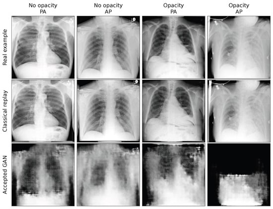
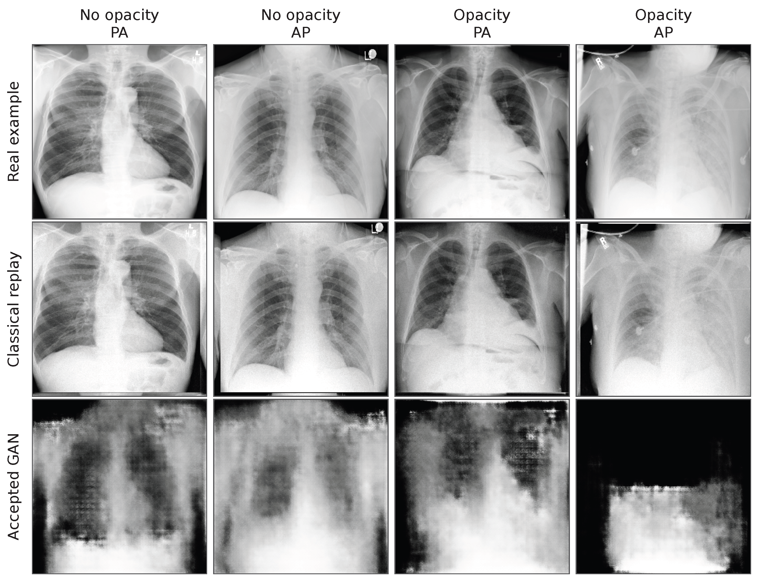
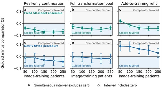
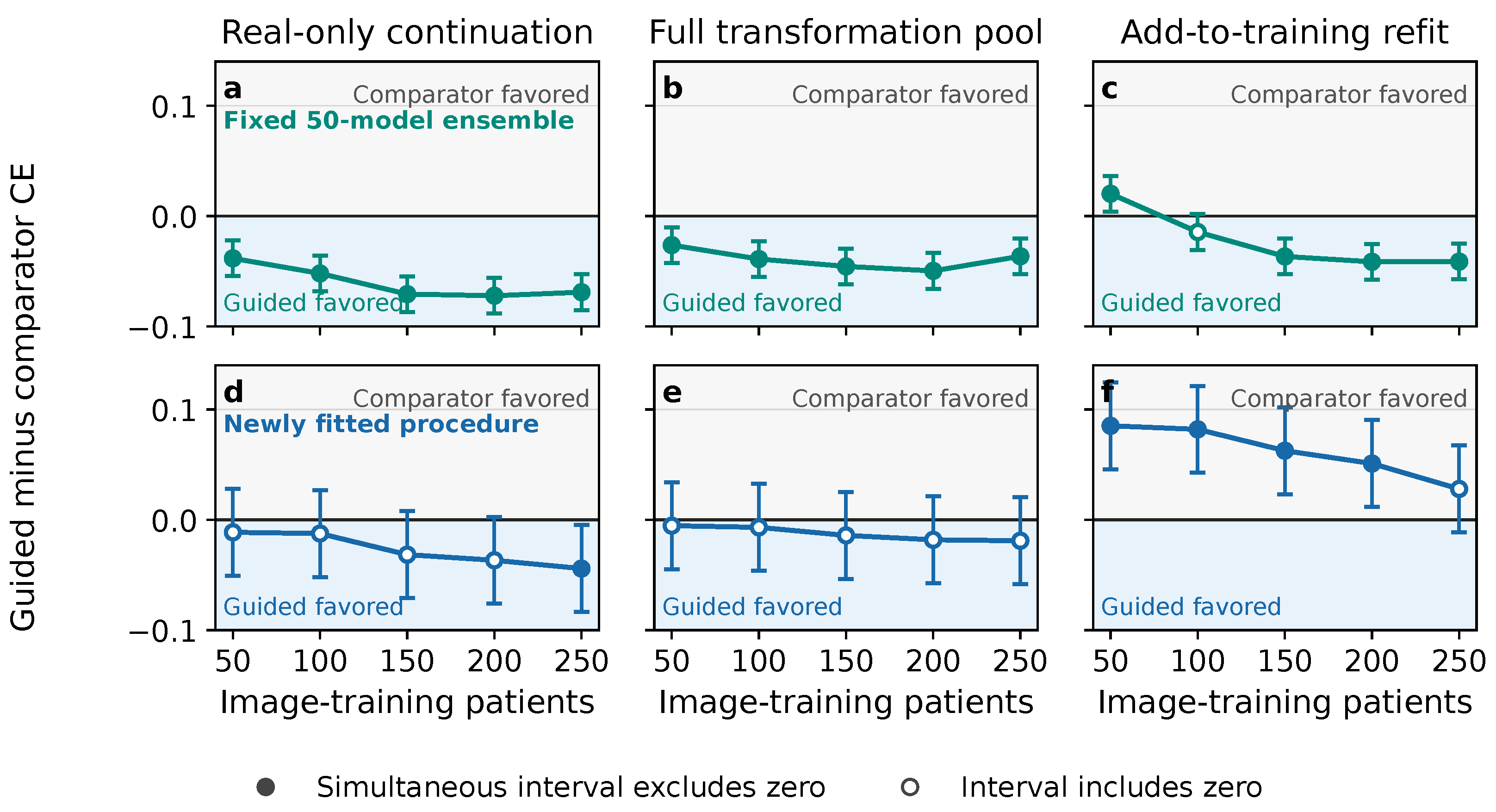

Disclaimer/Publisher’s Note: The statements, opinions and data contained in all publications are solely those of the individual author(s) and contributor(s) and not of MDPI and/or the editor(s). MDPI and/or the editor(s) disclaim responsibility for any injury to people or property resulting from any ideas, methods, instructions or products referred to in the content. |
© 2026 by the author. Licensee MDPI, Basel, Switzerland. This article is an open access article distributed under the terms and conditions of the Creative Commons Attribution (CC BY) license.