Dynamic Partner Retention, Network Dominance, and SME Productivity: A Statistical Modeling Approach

Abstract

Static concentration measures cannot show whether economically important trading relationships persist over time. This study constructs transaction-value-weighted measures of supplier and customer retention and incorporates them into a network-augmented model of firm productivity. Chinese value-added tax invoices and matched firm records from 2019 to 2025 yield an unbalanced panel of 443,506 firm–year observations. Supplier stability is the share of current purchases from suppliers retained from the preceding year, while customer stability is defined analogously using sales. Annual directed, weighted transaction networks are reconstructed from invoice flows, and DomiRank measures firms’ structural dominance. Total factor productivity is estimated using the Levinsohn–Petrin method. Firm and year fixed-effects estimates show negative relationships between both stability dimensions and productivity. Two-stage least-squares estimates using leave-one-out same-industry peer stability as instruments remain negative. Positive interactions with DomiRank indicate that stronger network positions attenuate these relationships. Potential operating-channel analyses associate stable ties with higher gross margins and asset turnover, but also with greater expenses, weaker operating profitability, slower inventory turnover, and longer operating cycles. Results are robust to alternative measures, matching, high-dimensional fixed effects, outlier treatment, lagged specifications, and industry–year stratified permutation tests. The findings show how longitudinal transaction statistics and network position jointly explain productivity heterogeneity among SMEs.

1. Introduction

Supplier and customer concentration indices summarize how transaction value is distributed among counterparties at a given point in time. They do not, however, reveal whether economically important partners remain in a firm’s transaction portfolio from one period to the next. Two firms may have similar concentration values even though one repeatedly trades with the same counterparties and the other reallocates comparable transaction shares to newly observed partners. This distinction creates a measurement problem in mathematical economics: the cross-sectional distribution of transaction value and the longitudinal persistence of exchange relationships are related but non-equivalent features of interfirm organization [1,2,3].

Digitized transaction records make this longitudinal dimension observable. Itemized value-added tax (VAT) invoices identify the counterparties, timing, and monetary value of realized exchanges and can be used to reconstruct interfirm networks [4]. More generally, research on production networks demonstrates the economic importance of observed buyer–supplier links [5,6]. Invoice records are particularly valuable for small and medium-sized enterprises (SMEs), which are rarely covered by major-partner disclosures. SME buyer–supplier relationships also raise questions about bargaining position and cash flow [7]; network connections and operating practices can be relevant to firm productivity [8].

Partner persistence has ambiguous economic implications. Repeated transactions may reduce search, contracting, monitoring, and coordination costs and may facilitate relationship-specific learning [9,10,11,12]. At the same time, continued reliance on incumbent counterparties can increase switching costs, deepen specific commitments, and expose a firm to hold-up or unfavorable trading terms [13,14,15]. These opposing mechanisms are especially relevant to SMEs because limited financial and organizational resources can restrict their ability to replace established partners.

A longitudinal retention statistic alone does not characterize the alternatives available to a firm. The same retention rate may imply severe dependence for a peripheral firm but a less restrictive commitment for a firm with broad access to other nodes. Research on supply networks consequently links structural position to access to information, innovation, resources, and operating performance [16,17,18]. A suitable statistical model should therefore combine local partner persistence with the focal firm’s position in the surrounding transaction network.

This study develops a network-augmented statistical modeling framework for that purpose. Supplier stability is defined as the share of current purchases attributable to suppliers retained from the preceding year, and customer stability is defined analogously using sales. Annual invoice flows are represented as directed, weighted networks, and DomiRank measures each firm’s structural dominance relative to its network neighborhood [19]. The framework then incorporates the two longitudinal retention statistics, DomiRank, and their interactions into a firm-level panel econometric model of total factor productivity (TFP).

The empirical analysis combines Chinese VAT invoices with business-registration and financial records from 2019 to 2025. After screening and matching, the unbalanced panel contains 443,506 firm–year observations. TFP is estimated using the Levinsohn–Petrin method [20]. Firm and year fixed effects account for time-invariant firm heterogeneity and common annual shocks, while firm-clustered standard errors accommodate within-firm dependence. Two-stage least squares using leave-one-out same-industry peer stability as instruments, matched samples, alternative measurements, high-dimensional fixed effects, different outlier treatments, and lagged specifications evaluate identification and model stability.

The fixed-effects estimates show significant negative relationships between supplier and customer stability and SME productivity. The instrumental-variable estimates based on peer stability instruments are also negative. Positive interactions between DomiRank and the two retention measures show that network dominance attenuates these negative relationships. Potential operating-channel analyses further associate persistent ties with higher gross margins and asset turnover but also with greater expenses, weaker operating profitability, slower inventory turnover, and longer operating cycles.

The study makes three contributions. First, it extends longitudinal partner measurement beyond disclosed major counterparties by using transaction-value-weighted retention statistics constructed from the full observed invoice portfolio. These statistics identify the share of current transactions attributable to continuing relationships rather than restricting measurement to a small set of major partners. Second, it integrates those statistics with a competition-based network measure in a conditional panel model, thereby connecting bilateral persistence to the structural alternatives represented by the wider network. Third, it combines large-scale transaction networks with panel econometrics and a comprehensive validation strategy to explain productivity heterogeneity among SMEs. The remainder of this paper develops the economic and statistical framework, describes the data and estimation strategy, reports the results and model-validation exercises, and discusses their implications.

2. Economic and Statistical Framework

2.1. Longitudinal Measurement of Partner Retention

Partner retention concerns whether the identities attached to economically important transaction shares persist between adjacent periods. It is therefore conceptually distinct from concentration, which describes the within-period distribution of transaction value across counterparties. Two firms can have similar concentration levels but very different patterns of partner continuity. Likewise, a diversified transaction portfolio can be either persistent or frequently reconfigured. Our longitudinal measures address this distinction by weighting retained relationships according to their current transaction values rather than assigning equal importance to every continuing counterparty. Section 3.3.2 presents the complete variable definitions, notation, and formulas.

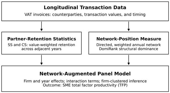
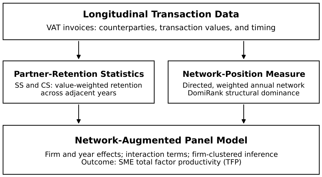
The same invoice records also define the annual weighted transaction network. Figure 1 summarizes how the transaction data are transformed into longitudinal retention statistics and a network-position measure and then incorporated into the panel model.

Figure 1. Network-augmented statistical modeling framework. Longitudinal VAT transaction records are used to construct transaction-value-weighted supplier and customer retention measures and annual directed, weighted interfirm networks. These longitudinal and network statistics are jointly incorporated into panel econometric models of SME total factor productivity.

2.2. Economic Implications of Partner Retention

Supplier and customer stability describe, respectively, the continued use of incumbent suppliers in purchasing and incumbent customers in sales. They are dynamic properties of exchange relationships rather than snapshots of transaction concentration [1,21]. This distinction matters because two firms with equally concentrated transactions may differ sharply in partner turnover: one may repeatedly transact with the same counterparties, while the other reallocates comparable transaction shares to new ones. Stability therefore captures the persistence of relational arrangements through which inputs, products, information, and payments move.

Its productivity implications reflect two countervailing mechanisms. Repeated exchange can save the costs of searching for and evaluating new counterparties, negotiating operating procedures, and monitoring performance [9]. Experience with a partner can also improve forecasting, quality control, scheduling, and the fit between technical interfaces. Over time, shared routines, complementary assets, and relationship-specific knowledge may support more efficient coordination [10,11,22,23]. Studies of listed firms report positive relationships of disclosed major-partner stability with financial performance or TFP [1,21]. Their samples and retention measures differ from the invoice-based SME measures analyzed here.

The same persistence can narrow a firm’s outside options. Because contracts cannot specify every future contingency, investments tailored to a particular counterparty generate quasi-rents after they are sunk [13,14]. A partner may appropriate part of those rents when the focal firm cannot switch without delay or loss. Resource dependence adds a second constraint: unequal access to critical inputs, sales outlets, or cash flows converts dependence into asymmetric influence [15]. Weak exit options may consequently expose a firm to price concessions, restrictive specifications, delayed payment, or inefficient commitments. Research on relationship-specific investment discusses both relational gains and hold-up risks [22]. In SMEs, supplier-specific investments have been associated with financing constraints [24]. Evidence on customer concentration and interfirm market-power disparities further links partner structure and bargaining asymmetry to financial performance, with relationships that need not be uniformly negative [25,26]. Evidence from international buyer–supplier relationships also shows that pandemic-related shocks can intensify conflict and buyer opportunism, illustrating another source of strain in ongoing exchanges [27].

The balance between these mechanisms should differ across firms. Large firms may diversify partners, enforce contractual safeguards, and absorb temporary switching costs. SMEs generally have thinner financial buffers, smaller procurement and sales teams, and fewer immediately available substitutes. Even when repeated exchange lowers routine coordination costs, dependence may impede the reallocation of inputs, capital, labor, and managerial attention. The hypotheses below therefore focus on the two sides of the supply chain separately.

2.2.1. Supplier Stability

Retaining suppliers familiarizes a buyer with input quality, delivery practices, and production interfaces. This knowledge can reduce inspection and adjustment needs and may limit short-term production uncertainty. Yet a high value-weighted retention rate also means that incumbent suppliers continue to account for a large share of current purchases. For an SME, this pattern can make production disproportionately reliant on a restricted set of input channels.

One consequence is weaker comparison and switching capacity. Alternative suppliers may require renewed certification, equipment calibration, trial production, or changes to logistics and inventory routines. Such costs reduce the credibility of the buyer’s threat to move purchases. Related research on supplier concentration discusses both transaction-cost savings and resource-dependence risks when firms rely on a narrower supplier base [28]. Under such dependence, an incumbent’s price increase, delivery delay, or quality deterioration can pass more readily into the focal firm’s production process. Limited substitution also reduces the flexibility with which inputs are reallocated when technologies or market conditions change.

A second consequence arises from supplier-specific investment. Technical interfaces, customized components, dedicated tooling, and process standards can improve the fit of an existing exchange, but their value is often lower outside that relationship [13,14,22]. As these commitments accumulate, the buyer may remain tied to an established input configuration even when more efficient technologies become available. Evidence concerning SME relationship-specific investment points to associated hold-up and financing risks [24], while research on supplier-base concentration discusses how limited knowledge diversity and fewer alternative sources can constrain innovation [29].

Finally, continuity may require buffers and administrative effort. Safety inventories, synchronized delivery plans, relationship maintenance, and adaptation to supplier requirements can preserve production in the short run but absorb working capital and managerial attention. Related evidence links supplier-base concentration to higher precautionary cash holdings, particularly when inventory efficiency is low, and higher cash spending on R&D [30]. Supplier concentration and partner retention describe different features of the transaction portfolio, but this evidence illustrates the liquidity considerations that may accompany reliance on established input channels. We therefore expect the loss of flexibility and the resource burden associated with supplier dependence to outweigh the coordination benefit in the SME sample.

Hypothesis 1. 

Supplier stability reduces total factor productivity among SMEs.

2.2.2. Customer Stability

Continuing customers can reduce marketing and demand-forecasting costs and provide recurring orders. They may also convey product feedback that improves scheduling and quality. Nevertheless, a high value-weighted customer-retention rate indicates that a substantial share of current revenue continues to come from established buyers. When replacement orders are difficult to obtain, these buyers influence not only sales volume but also cash-flow timing and the deployment of productive resources.

First, a weak outside option may lead an SME to accept price concessions, tighter quality tolerances, shorter delivery schedules, or additional services. Relationship-specific investments make termination more costly and can strengthen the customer’s ability to capture value [13,15,31]. Research on customer concentration finds that its association with supplier profitability can be nonlinear [32]; evidence on market-power discrepancies more directly connects asymmetric power with weaker financial performance [26]. The resulting pressure can reduce funds available for productivity-enhancing investment even when order volume remains stable.

Second, investments tailored to a particular customer can be difficult to redeploy when that customer’s specifications or demand change [24]. A persistent customer portfolio may also expose the firm to a narrower range of demand signals and product standards, weakening learning from other markets. This information constraint is distinct from immediate bargaining pressure but can similarly slow product and process adaptation.

Third, payment practices link customer dependence to financing. Powerful buyers can extend settlement periods, shifting working-capital needs to SME suppliers. Evidence on trade credit shows that customer payment behavior affects receivables and financing constraints, while greater transparency can alter the underlying bargaining relationship [33,34]. For firms with limited external finance, cash tied up in established customer relationships may crowd out equipment, research, or training expenditure. Order continuity may thus be accompanied by customization, information, and liquidity costs [25,26].

Hypothesis 2. 

Customer stability reduces total factor productivity among SMEs.

2.3. Network Dominance and Conditional Productivity Relationships

The costs embedded in a stable dyad depend on the opportunities available beyond that dyad. A bilateral retention rate does not indicate whether the focal firm can reach other suppliers or customers, obtain comparable resources elsewhere, or learn about alternative technologies and markets. Network location and supply-base structure have been linked to firms’ access to knowledge, innovation, and productivity [3,35,36,37,38,39]. Firms with similar stability may therefore experience different constraints when their positions in the surrounding transaction system differ.

DomiRank identifies structural dominance through competition among connected nodes [19]. Unlike a simple partner count, it evaluates a node relative to the structure of its neighborhood. A high score is not direct evidence of contractual bargaining power or product-market power; rather, it denotes a structural position that may provide wider access to information, resources, and potential counterparties. This distinction allows the statistical model to test whether network position conditions the productivity implications of local relationship continuity.

Resource dependence theory provides the first rationale for moderation. Dependence on an incumbent is lower when comparable resources can be obtained from other actors [15]. A structurally dominant firm may have more visible or accessible alternatives and may therefore reconfigure purchases or sales with less disruption. In incomplete-contract terms, that credible possibility of rematching lowers the expected return to exploiting sunk relationship-specific investments [13,14]. Network position need not eliminate dependence; it changes the options available when an established relationship becomes restrictive.

On the purchasing side, broader network reach can reveal substitute inputs, technical information, and alternative suppliers. It also improves the firm’s basis for comparing prices and quality. The ability to reorganize sourcing makes unilateral dependence on an incumbent’s standards or delivery system less binding. Network dominance should accordingly reduce the input lock-in associated with supplier continuity.

Hypothesis 3. 

Network dominance mitigates the negative effect of supplier stability on total factor productivity among SMEs.

On the sales side, network reach can broaden demand information and potential market outlets. A firm with credible alternative customers is better placed to resist price reductions, extended payment periods, or costly customization requirements. Related evidence finds that network dominance moderates the productivity relationship of supplier and customer concentration, a distinct measure of partner structure [3]. We therefore expect it to weaken the negative relationship on the customer side as well.

Hypothesis 4. 

Network dominance mitigates the negative effect of customer stability on total factor productivity among SMEs.

3. Data and Statistical Methodology

3.1. Data and Sample Construction

The database combines digitized itemized VAT invoices with business-registration, tax-return, and financial-statement records. Each invoice identifies both parties, the transaction date, and its value, permitting the recovery of partner sets, relationship continuity, and the economic weight of individual links. Unlike major-partner disclosures, these records cover a broad range of transactions and support the reconstruction of firm-level production networks from a common relational source [4]. The invoices improve the researcher’s ability to observe the transaction system; they are not used as a proxy for the digital maturity or technology-adoption decisions of individual firms.

We remove voided invoices, unidentified counterparties, self-transactions, nonpositive values, and other evidently abnormal records, then aggregate valid values by firm, counterparty, and year. Financial and real-estate firms are omitted because their accounting and input structures differ from those of nonfinancial firms. Firm–years lacking the information required for the principal variables or containing logical inconsistencies are also excluded. Continuous variables are winsorized at the 1st and 99th percentiles.

The raw records span 2019–2025; the first year supplies the lagged partner sets needed for the initial retention measures. SMEs are classified with the industry-specific employment, revenue, and asset thresholds in China’s official Provisions on the Classification Standards for Small and Medium-Sized Enterprises (MIIT Joint Enterprise [2011] No. 300). The final unbalanced panel contains 443,506 firm–year observations.

3.2. Directed Weighted Transaction Network

For each year, firms form the nodes of a directed, weighted transaction network [40,41]. If supplier u sells to customer v, $w_{uv,t}$ equals their annual aggregate invoice value. Self-links, unidentified parties, and nonpositive links are removed. The baseline network retains all remaining positive annual firm-pair transactions and therefore imposes no additional minimum transaction-value threshold. To assess whether small-value links materially affect network topology and the resulting DomiRank scores, we reconstruct the annual networks using minimum transaction values of CNY 1000 , CNY 2000, and CNY 5000 in the sensitivity analysis. These thresholds apply only to network construction; supplier and customer stability are calculated from all cleaned valid invoice records.

The network is not restricted to regression-sample SMEs. It includes every valid interfirm transaction available in a given year, and DomiRank is calculated for all observed nodes before scores are matched to the SME panel. This broader boundary avoids mechanically truncating each SME’s network environment.

3.3. Variable Definitions

3.3.1. Dependent Variable: Total Factor Productivity

TFP represents output differences not accounted for by measured capital, labor, and intermediate inputs [42,43]. We begin with the Cobb–Douglas specification

$$\ln \left(Y_{it}\right)=\alpha \ln \left(L_{it}\right)+\beta \ln \left(K_{it}\right)+\gamma \ln \left(M_{it}\right)+{\delta }_t+{\omega }_{it}+{\epsilon }_{it}.$$

(1)

Here, $Y_{it}$ is operating revenue, $L_{it}$ is the number of employees, $K_{it}$ is net fixed assets, and $M_{it}$ is cash paid for goods and services. Year effects are denoted by ${\delta }_t$, latent firm productivity by ${\omega }_{it}$, and the idiosyncratic disturbance by ${\epsilon }_{it}$. Operating revenue is used as the output measure because consistent physical-output quantities are unavailable for the multi-industry SME sample. Employee headcount measures labor quantity, net fixed assets represent the productive capital stock, and cash paid for goods and services captures flexible expenditure on purchased materials and services. Prior productivity research has compared wage bills with employment counts as alternative labor-input measures [44]; we use employee headcount for the labor term. Because a firm’s intermediate-input choices can respond to productivity observed by the firm but not the researcher, we use intermediate inputs as the proxy in the Levinsohn–Petrin estimator and take the recovered ${\omega }_{it}$ as TFP [20].

3.3.2. Core Explanatory Variables: Supplier and Customer Stability

Previous studies have measured relationship persistence using disclosed major suppliers and customers. Some use the overlap of partner identities across years [21,45]. Gu et al. instead construct a transaction-share-weighted index for the top five suppliers and customers, summing the smaller of each continuing partner’s shares in adjacent years [1]. These approaches establish the distinction between stability and within-period concentration, but the disclosure-based measures cover only major counterparties.

Building on this literature, we use VAT invoices to calculate partner-retention rates over all observed valid transactions. Unlike Gu et al.’s minimum-of-two-years share for each continuing top-five partner, our numerator sums current-year transaction values with partners also observed in the preceding year, and our denominator is the firm’s total current purchases or sales across all observed partners. The resulting measures emphasize economically important continuing relationships in the current portfolio while limiting the influence of incidental small-value transactions. Supply chain stability is measured separately from the purchasing and sales sides as supplier stability and customer stability.

Supplier stability (${\mathit{SS}}_{it}$) is the proportion of a firm’s current purchases sourced from suppliers that traded with the firm in both the current and preceding years:

$${\mathit{SS}}_{i,t}={\displaystyle \frac{{\displaystyle \sum _{j\in (S_{i,t}\cap S_{i,t-1})}{\mathit{Purchase}}_{i,j,t}}}{{\displaystyle \sum _{k\in S_{i,t}}{\mathit{Purchase}}_{i,k,t}}}},$$

(2)

where $S_{i,t}$ is the set of firm i’s suppliers in year t, and $S_{i,t}\cap S_{i,t-1}$ is the set of retained suppliers from which the firm made purchases in both years $t-1$ and t. ${\mathit{Purchase}}_{i,j,t}$ denotes the invoice value of purchases made by firm i from supplier j in year t. ${\mathit{SS}}_{i,t}$ ranges from zero to one, with a higher value indicating that retained suppliers account for a larger proportion of the firm’s current purchasing activity.

Customer stability (${\mathit{CS}}_{it}$) is the proportion of a firm’s current sales attributable to customers that traded with the firm in both the current and preceding years:

$${\mathit{CS}}_{i,t}={\displaystyle \frac{{\displaystyle \sum _{m\in (C_{i,t}\cap C_{i,t-1})}{\mathit{Sales}}_{i,m,t}}}{{\displaystyle \sum _{n\in C_{i,t}}{\mathit{Sales}}_{i,n,t}}}},$$

(3)

where $C_{i,t}$ is the set of firm i’s customers in year t, and $C_{i,t}\cap C_{i,t-1}$ is the set of retained customers that purchased from the firm in both years $t-1$ and t. ${\mathit{Sales}}_{i,m,t}$ denotes the invoice value of sales from firm i to customer m in year t. ${\mathit{CS}}_{i,t}$ also ranges from zero to one, with a higher value indicating greater continuity of existing customer relationships in the firm’s current sales activity.

Both measures are calculated from all valid transactions remaining after the cleaning rules described above. The alternative minimum-value thresholds used in the network sensitivity analysis are not imposed on the retention measures. This separation prevents network-preprocessing choices from mechanically determining the longitudinal explanatory variables.

3.3.3. Moderating Variable: Network Dominance

Centrality measures embody different network mechanisms [40,41,46]. PageRank recursively transfers prestige from highly ranked neighbors and is well suited to endorsement or information flows [47,48]. DomiRank instead models competition: the dominance acquired by one node suppresses that of adjacent nodes, making it suitable for locating firms relative to competitors in their transaction neighborhood [19]. It is therefore a competition-oriented alternative, not a direct algebraic extension of PageRank.

Following the formulation in [19], let ${\mathbf{A}}_t\in {\mathbb{R}}^{N_t\times N_t}$ be the directed, weighted adjacency matrix in year t. Taking the delivery of goods or services as the direction of resource flow, a sale from supplier u to customer v is represented by the resource-flow edge $u\to v$ with annual transaction value $w_{uv,t}$. Directed DomiRank is calculated on the reverse of this resource-flow graph; therefore, purchasers occupy rows, sellers occupy columns, and $A_{vu,t}=w_{uv,t}$. This orientation makes a firm’s score depend on the suppliers in its transaction neighborhood, consistent with the competitive resource-acquisition interpretation of DomiRank. The score dynamics are

$${\displaystyle \frac{d{\mathbf{\Gamma }}_t\left(\tau \right)}{d\tau }}=\alpha {\mathbf{A}}_t\left[\theta \mathbf{1}-{\mathbf{\Gamma }}_t\left(\tau \right)\right]-\beta {\mathbf{\Gamma }}_t\left(\tau \right),$$

(4)

where $\alpha >0$ governs the acquisition of dominance from the network neighborhood, $\beta >0$ is the decay rate, and $\theta >0$ is a scale parameter. With $\sigma =\alpha /\beta$, the steady state obeys

$$\left(\sigma {\mathbf{A}}_t+\mathbf{I}\right){\mathbf{\Gamma }}_t=\theta \sigma {\mathbf{A}}_t\mathbf{1},$$

(5)

and hence

$${\mathbf{\Gamma }}_t=\theta \sigma {\left(\sigma {\mathbf{A}}_t+\mathbf{I}\right)}^{-1}{\mathbf{A}}_t\mathbf{1}.$$

(6)

Equation (6) is an analytical representation; the empirical implementation does not form a dense matrix inverse. For each candidate value of $\sigma$, we solve the sparse linear system in Equation (5) using the biconjugate gradient stabilized (BiCGSTAB) algorithm on a compressed sparse row representation of ${\mathbf{A}}_t$, with a relative convergence tolerance of ${10}^{-5}$.

Because ${\mathbf{A}}_t$ is directed and generally asymmetric, its eigenvalues need not be purely real. We retain the directed matrix and define

$${\lambda }_{\min }^{\Re }\left({\mathbf{A}}_t\right)=\underset{\lambda \in \mathrm{spec}\left({\mathbf{A}}_t\right)}{\min }\Re \left(\lambda \right),$$

(7)

that is, the smallest real part among the eigenvalues of ${\mathbf{A}}_t$. The Jacobian of Equation (4) is $-\beta (\mathbf{I}+\sigma {\mathbf{A}}_t)$. Asymptotic stability therefore requires $1+\sigma \Re \left(\lambda \right)>0$ for every $\lambda \in \mathrm{spec}\left({\mathbf{A}}_t\right)$. The computed value of ${\lambda }_{\min }^{\Re }\left({\mathbf{A}}_t\right)$ is negative for each annual network. Setting $\theta =1$, we define ${\sigma }_{\max ,t}=-1/{\lambda }_{\min }^{\Re }\left({\mathbf{A}}_t\right)$ and restrict the search to

$$0<\sigma <{\sigma }_{\max ,t}=-{\displaystyle \frac{1}{{\lambda }_{\min }^{\Re }\left({\mathbf{A}}_t\right)}}.$$

(8)

Equation (8) is the directed-network implementation of the original DomiRank convergence restriction. The adjacency matrix is not symmetrized when the scores are calculated.

For the baseline calculation, we evaluate $Q=100$ equally spaced interior candidate values over $(0,{\sigma }_{\max ,t})$, excluding both endpoints. For each candidate, nodes are removed according to the fixed descending order of their initially computed DomiRank scores; the scores are not recomputed after each removal. Network fragmentation is evaluated by plotting the relative size of the largest weakly connected component against the removed-node share. Equivalently, the component size is calculated on the unweighted, undirected projection solely for this evaluation; ${\mathbf{A}}_t$ remains directed and weighted when DomiRank scores are computed. The candidate that minimizes the area under the fragmentation curve is selected for the corresponding annual network. To assess the sensitivity of this numerical choice, the search is repeated with $Q=50$ and $Q=200$. To improve numerical readability, the annual raw scores are normalized and rescaled as

$${\mathit{DomiRank}}_{it}={10}^5{\displaystyle \frac{{\Gamma }_{it}}{{\displaystyle {\displaystyle \sum _{r=1}^{N_t}}{\Gamma }_{rt}}}}.$$

(9)

For each year, the transformation sets the sum of the reported scores to ${10}^5$. Because it multiplies all annual raw scores by the same positive scalar, it preserves their within-year ordering and changes only the reporting unit; regression coefficients consequently reflect the rescaled unit. ${\mathit{DomiRank}}_{it}$ denotes structural dominance in the observed VAT transaction network rather than contractual bargaining power, product-market share, or conventional market power.

3.3.4. Control Variables

The regressions account for firm resources, financial condition, growth, inputs, and market structure. $\mathit{Size}$ is the log of total assets and captures scale, financing capacity, and organizational complexity [8,43]. $\mathit{Age}$ is the log of one plus years since establishment and represents life-cycle experience and renewal [49]. $\mathit{Lev}$, total liabilities divided by total assets, reflects financing structure and constraints [50]. $\mathit{ROA}$ is net profit divided by total assets and controls for operating performance [25,26]. $\mathit{Growth}$ is the logarithmic growth rate of operating revenue, calculated as $\ln \left({\mathit{OperatingRevenue}}_{it}\right)-\ln \left({\mathit{OperatingRevenue}}_{i,t-1}\right)$, and captures firm expansion or contraction. Corporate taxation is relevant to firms’ investment decisions [51]; here, $\mathit{Tax}$ is measured as taxes paid divided by total assets. Labor cost intensity ($\mathit{LCI}$) is wage expenditure divided by total assets. Research and development intensity ($\mathit{R}\&\mathit{D}$) is R&D expenditure divided by operating revenue [52]. Finally, $\mathit{HHI}$ is the sum of squared firm sales shares within each province–industry–year market and controls for competitive structure [53,54].

3.4. Panel Econometric Models

3.4.1. Baseline Model

To estimate the within-firm relationships between partner retention and SME TFP, we use the following two-way fixed-effects model:

$$\begin{array}{cc}\hfill {\mathit{TFP}}_{ijst}=& {\alpha }_i+{\delta }_t+{\beta }_1{\mathit{SS}}_{ijst}+{\beta }_2{\mathit{CS}}_{ijst}+{\beta }_3{\mathit{Size}}_{ijst}+{\beta }_4{\mathit{Age}}_{ijst}\hfill \\ \hfill & +{\beta }_5{\mathit{Lev}}_{ijst}+{\beta }_6{\mathit{ROA}}_{ijst}+{\beta }_7{\mathit{Growth}}_{ijst}+{\beta }_8{\mathit{Tax}}_{ijst}\hfill \\ \hfill & +{\beta }_9{\mathit{LCI}}_{ijst}+{\beta }_{10}\mathit{R}\&{\mathit{D}}_{ijst}+{\beta }_{11}{\mathit{HHI}}_{jst}+{\epsilon }_{ijst}.\hfill \end{array}$$

(10)

Here, i, j, s, and t denote the firm, industry, province, and year, respectively. ${\alpha }_i$ represents firm fixed effects, which control for time-invariant firm heterogeneity. ${\delta }_t$ represents year fixed effects, which absorb annual macroeconomic shocks common to all firms. ${\epsilon }_{ijst}$ is the error term. Supplier stability and customer stability are included simultaneously to estimate their respective within-firm coefficients from the purchasing and sales sides. Standard errors are clustered at the firm level to accommodate heteroskedasticity and within-firm dependence.

Consistent with Hypotheses 1 and 2, we expect ${\beta }_1<0$ and ${\beta }_2<0$.

3.4.2. Moderation Model

To test the moderating role of network dominance, we augment the baseline specification by including DomiRank and its interactions with supplier stability and customer stability:

$$\begin{array}{cc}\hfill {\mathit{TFP}}_{ijst}=& {\alpha }_i+{\delta }_t+{\beta }_1{\mathit{SS}}_{ijst}+{\beta }_2{\mathit{CS}}_{ijst}+{\beta }_3{\mathit{DomiRank}}_{ijst}\hfill \\ \hfill & +{\beta }_4\left({\mathit{SS}}_{ijst}\times {\mathit{DomiRank}}_{ijst}\right)+{\beta }_5\left({\mathit{CS}}_{ijst}\times {\mathit{DomiRank}}_{ijst}\right)\hfill \\ \hfill & +{\beta }_6{\mathit{Size}}_{ijst}+{\beta }_7{\mathit{Age}}_{ijst}+{\beta }_8{\mathit{Lev}}_{ijst}+{\beta }_9{\mathit{ROA}}_{ijst}\hfill \\ \hfill & +{\beta }_{10}{\mathit{Growth}}_{ijst}+{\beta }_{11}{\mathit{Tax}}_{ijst}+{\beta }_{12}{\mathit{LCI}}_{ijst}\hfill \\ \hfill & +{\beta }_{13}\mathit{R}\&{\mathit{D}}_{ijst}+{\beta }_{14}{\mathit{HHI}}_{jst}+{\epsilon }_{ijst}.\hfill \end{array}$$

(11)

The interaction term ${\mathit{SS}}_{ijst}\times {\mathit{DomiRank}}_{ijst}$ tests whether network dominance moderates the effect of supplier stability on SME TFP, whereas ${\mathit{CS}}_{ijst}\times {\mathit{DomiRank}}_{ijst}$ tests whether network dominance moderates the effect of customer stability on SME TFP. The corresponding marginal effects are

$${\displaystyle \frac{\partial {\mathit{TFP}}_{ijst}}{\partial {\mathit{SS}}_{ijst}}}={\beta }_1+{\beta }_4{\mathit{DomiRank}}_{ijst},$$

(12)

and

$${\displaystyle \frac{\partial {\mathit{TFP}}_{ijst}}{\partial {\mathit{CS}}_{ijst}}}={\beta }_2+{\beta }_5{\mathit{DomiRank}}_{ijst}.$$

(13)

Consistent with Hypotheses 3 and 4, attenuation of the negative conditional relationships requires ${\beta }_4>0$ and ${\beta }_5>0$. Equations (12) and (13) are evaluated at the 10th, 25th, 50th, 75th, and 90th percentiles of DomiRank.

3.5. Identification and Statistical Inference

The fixed-effects transformation removes time-invariant firm characteristics, and year effects absorb shocks common to all firms. To address concerns about reverse causality, time-varying omitted variables, and measurement error, we complement the baseline model with two-stage least squares using leave-one-out same-industry peer stability as instruments, as defined in Section 4.3.1. The peer measures capture industry-level relational conditions while excluding the focal firm’s own value from their construction. Reported first-stage F statistics evaluate instrument relevance, the Kleibergen–Paap rk LM statistic tests underidentification, and the Wu–Hausman statistic evaluates whether the endogenous-regressor specification differs systematically from the corresponding fixed-effects estimator.

Propensity-score matching reduces observable differences between firms with high and low retention. Alternative TFP, retention, and network-position measures assess measurement sensitivity, while different outlier rules, high-dimensional fixed effects, and lagged specifications evaluate specification dependence. All reported regression standard errors are clustered at the firm level.

4. Empirical Results

4.1. Descriptive Statistics

Table 1 summarizes the analysis sample. Mean TFP is 6.5903 (SD 0.8067). Retained partners account, on average, for 61.95% of current purchases and 64.72% of current sales. The dispersion in both retention rates supplies useful identifying variation. DomiRank is right-skewed (mean 0.0707; SD 0.1324), indicating that structural dominance is concentrated among a comparatively small group of firms.

Table 1. Descriptive statistics.

Variable	Mean	SD	Minimum	P25	Median	P75	Maximum
$\mathit{TFP}$	6.5903	0.8067	4.5595	6.0573	6.5781	7.1027	8.8353
$\mathit{SS}$	0.6195	0.2651	0.0102	0.4369	0.6707	0.8380	0.9951
$\mathit{CS}$	0.6472	0.2705	0.0187	0.4567	0.7059	0.8780	0.9980
$\mathit{DomiRank}$	0.0707	0.1324	0.0017	0.0092	0.0241	0.0689	0.8752
$\mathit{Size}$	6.9448	1.5503	2.6858	5.9229	6.9567	7.9648	10.7144
$\mathit{Age}$	2.1591	0.5945	0.6931	1.7918	2.1972	2.6391	3.3673
$\mathit{Lev}$	0.7347	0.3099	0.0071	0.5401	0.7647	0.9461	1.6187
$\mathit{ROA}$	0.0122	0.1108	−0.4815	−0.0092	0.0116	0.0438	0.4573
$\mathit{Growth}$	0.1192	0.2568	−0.6375	−0.0271	0.1182	0.2641	0.9024
$\mathit{Tax}$	0.0366	0.0607	0.0000	0.0064	0.0188	0.0419	0.4528
$\mathit{LCI}$	0.1722	0.3611	0.0000	0.0322	0.0773	0.1665	2.9056
R&D	0.0098	0.0323	0.0000	0.0000	0.0000	0.0000	0.2074
$\mathit{HHI}$	0.0180	0.0362	0.0008	0.0025	0.0063	0.0150	0.2390

Notes: The sample contains $N=\mathrm{443,506}$ firm–year observations. All continuous variables are winsorized at the 1st and 99th percentiles.

4.2. Baseline Panel Estimates

Column (1) of Table 2 reports the control-variable specification with year fixed effects. Column (2) adds supplier and customer stability and absorbs firm fixed effects, while Column (3), the preferred specification, includes both firm and year fixed effects. In Column (3), the coefficients are $-0.0645$ for supplier stability and $-0.0740$ for customer stability; both are significant at the 1% level. A one-standard-deviation increase corresponds to 0.0171 and 0.0200 lower log TFP, respectively. These within-firm estimates support Hypotheses 1 and 2 and indicate that dependence-related constraints outweigh coordination gains in the SME sample. In contrast, Gu et al. report a positive relationship between major-partner stability and financial performance among Chinese listed firms [1]; differences in sample, outcome, and retention measurement are relevant when comparing the findings.

Table 2. Supply chain stability and SME total factor productivity: Baseline results.

	(1)	(2)	(3)
Variable	Controls Only	Firm FE	Two-Way FE
$\mathit{SS}$		$-0.0677$ ***	$-0.0645$ ***
		$(-17.969)$	$(-14.255)$
$\mathit{CS}$		$-0.0750$ ***	$-0.0740$ ***
		$(-19.477)$	$(-16.003)$
$\mathit{Size}$	$0.0305$ ***	$0.0384$ ***	$0.0315$ ***
	$\left(9.738\right)$	$\left(14.804\right)$	$\left(10.027\right)$
$\mathit{Age}$	$0.1659$ ***	$-0.1158$ ***	$0.1931$ ***
	$\left(15.148\right)$	$(-21.898)$	$\left(17.498\right)$
$\mathit{Lev}$	$0.0879$ ***	$0.0827$ ***	$0.0855$ ***
	$\left(10.504\right)$	$\left(11.888\right)$	$\left(10.207\right)$
$\mathit{ROA}$	$0.7295$ ***	$0.7196$ ***	$0.7259$ ***
	$\left(48.747\right)$	$\left(58.103\right)$	$\left(48.560\right)$
$\mathit{Growth}$	$-0.0030$	$-0.0024$	$-0.0029$
	$(-0.981)$	$(-0.933)$	$(-0.923)$
$\mathit{Tax}$	$2.0588$ ***	$2.1070$ ***	$2.0677$ ***
	$\left(46.038\right)$	$\left(56.585\right)$	$\left(46.143\right)$
$\mathit{LCI}$	$-0.0663$ ***	$-0.0720$ ***	$-0.0648$ ***
	$(-7.203)$	$(-9.413)$	$(-7.020)$
R&D	$-0.0775$ **	$0.3605$ ***	$-0.0736$ **
	$(-2.310)$	$\left(13.726\right)$	$(-2.198)$
$\mathit{HHI}$	$-0.3484$ ***	$-0.2626$ ***	$-0.3516$ ***
	$(-5.203)$	$(-4.810)$	$(-5.249)$
Firm fixed effects	NO	YES	YES
Year fixed effects	YES	NO	YES
Observations	443,506	443,506	443,506
Within $R^2$	$0.0468$	$0.0726$	$0.0507$

Notes: The table reports t-statistics in parentheses. Standard errors are clustered at the firm level. ***, **, and * indicate statistical significance at the 1%, 5%, and 10% levels, respectively.

4.3. Instrumental-Variable and Matched-Sample Estimates

4.3.1. Instrumental-Variable Estimation

Reverse causality and time-varying omitted factors may jointly influence partner retention and productivity. We therefore estimate a two-stage least-squares specification using peer stability instruments. Related studies use peer averages of supplier and customer concentration [3], regional peer averages of partner stability [21], or instruments incorporating an industry-level customer-stability measure [55]. These precedents motivate the use of peer information, although none uses exactly the two leave-one-out, same-four-digit-industry–year stability instruments constructed here. The estimation follows the standard instrumental-variable framework [56]. For each firm–year, the peer group comprises all other sample firms in the same four-digit industry and year. The focal firm is excluded from the group mean. Let ${\mathcal{G}}_{g\left(i\right),t}$ denote the set of firms in firm i’s four-digit industry $g\left(i\right)$ in year t, and let $N_{g\left(i\right),t}$ denote the number of firms in that group. The supplier-side instrument is

$${\mathit{PeerSS}}_{it}={\displaystyle \frac{{\displaystyle \sum _{k\in {\mathcal{G}}_{g\left(i\right),t},k\ne i}{\mathit{SS}}_{kt}}}{N_{g\left(i\right),t}-1}},$$

(14)

and the customer-side instrument is

$${\mathit{PeerCS}}_{it}={\displaystyle \frac{{\displaystyle \sum _{k\in {\mathcal{G}}_{g\left(i\right),t},k\ne i}{\mathit{CS}}_{kt}}}{N_{g\left(i\right),t}-1}}.$$

(15)

These contemporaneous leave-one-out means are simple arithmetic averages rather than transaction-value-weighted peer aggregates. Their relevance follows from shared industry-level contracting practices, production technologies, partner availability, and relationship norms, which can generate common patterns of supplier and customer retention. Excluding firm i prevents its own stability value from entering its instrument mechanically. The exclusion restriction requires that, conditional on firm and year fixed effects and the observed controls, peer stability affects the focal firm’s productivity through the focal firm’s own supplier and customer stability rather than through an independent channel.

Table 3 reports both stages. In the supplier-stability first stage, the coefficients of $\mathit{PeerSS}$ and $\mathit{PeerCS}$ are 0.2140 and 0.0402; in the customer-stability first stage, they are 0.0330 and 0.1994. The reported first-stage F statistics are 140.92 and 111.56, and the Kleibergen–Paap rk LM test rejects underidentification ($p<0.001$). In the second stage, supplier and customer stability have coefficients of $-0.2086$ and $-0.2888$, significant at the 10% and 5% levels, respectively. The Wu–Hausman test also rejects exogeneity ($p<0.001$). Subject to the peer-instrument exclusion restriction, the 2SLS estimates support negative relationships between supplier and customer stability and productivity.

Table 3. Instrumental-variable estimates.

	(1)	(2)	(3)
Variable	$\mathit{SS}$	$\mathit{CS}$	$\mathit{TFP}$
$\mathit{SS}$			$-0.2086$ *
			$(-1.66)$
$\mathit{CS}$			$-0.2888$ **
			$(-2.12)$
$\mathit{PeerSS}$	$0.2140$ ***	$0.0330$ **
	$\left(14.79\right)$	$\left(2.41\right)$
$\mathit{PeerCS}$	$0.0402$ ***	$0.1994$ ***
	$\left(2.95\right)$	$\left(13.44\right)$
Control variables	YES	YES	YES
Firm fixed effects	YES	YES	YES
Year fixed effects	YES	YES	YES
Wu–Hausman F statistic			$24.5654$
Wu–Hausman p-value			<0.001
K–P rk LM statistic			14,439.4308
K–P rk LM p-value			<0.001
First-stage F statistic ($\mathit{SS}$ equation)			$140.92$
First-stage F statistic ($\mathit{CS}$ equation)			$111.56$
Observations	443,506	443,506	443,506
Within $R^2$	$0.0326$	$0.0340$	$0.0441$

Notes: Columns (1) and (2) present the first-stage estimates, and Column (3) presents the second-stage estimate. $\mathit{PeerSS}$ and $\mathit{PeerCS}$ are contemporaneous leave-one-out arithmetic means of supplier and customer stability among other firms in the same four-digit industry and year. The table reports t-statistics in parentheses. Standard errors are clustered at the firm level. ***, ** and * indicate statistical significance at the 1%, 5%, and 10% levels, respectively.

The 2SLS coefficients are larger in absolute value than the fixed-effects estimates. This difference does not imply that the IV estimates are mechanically more accurate. Measurement error in the retention variables can attenuate fixed-effects coefficients, while 2SLS uses only the component of firm retention predicted by same-industry peer stability. The resulting 2SLS coefficient draws on variation in retention predicted by the peer instruments and need not equal the average within-firm association for the full sample [56]. Heterogeneous responses can contribute to differences in magnitude, although they do not by themselves establish why the estimates differ. At the same time, any direct effect of unobserved industry–year conditions on focal-firm productivity would also affect the 2SLS estimates. We therefore emphasize the sign consistency across estimators and interpret the IV magnitudes conditional on the exclusion restriction.

4.3.2. Propensity-Score-Matched Sample Analysis

As a complementary robustness test, we match firms above and below the industry–year median of each stability measure. A logit model uses size, age, leverage, ROA, growth, tax burden, labor cost intensity, R&D intensity, HHI, and industry and year indicators. One-to-one nearest-neighbor matching on common support yields 340,904 supplier-stability and 341,312 customer-stability observations. The maximum absolute standardized mean difference falls from 25.03% to 0.47% in the supplier-stability match and from 20.86% to 0.52% in the customer-stability match; every matched covariate is below the conventional 10% threshold. As shown in Table 4, the two-way fixed-effects estimates remain negative and significant in both matched samples, showing that observable sample composition does not explain the main findings.

Table 4. Propensity-score-matched estimates and balance diagnostics.

	(1)	(2)
Variable	$\mathit{TFP}$ ($\mathit{SS}$ Match)	$\mathit{TFP}$ ($\mathit{CS}$ Match)
$\mathit{SS}$	$-0.0606$ ***	$-0.0582$ ***
	$(-9.228)$	$(-9.038)$
$\mathit{CS}$	$-0.0684$ ***	$-0.0635$ ***
	$(-10.187)$	$(-9.409)$
Control variables	YES	YES
Firm fixed effects	YES	YES
Year fixed effects	YES	YES
Observations	340,904	341,312
Within $R^2$	$0.0458$	$0.0521$
Max. $\left|\mathrm{SMD}\right|$ before matching	$25.03\%$	$20.86\%$
Max. $\left|\mathrm{SMD}\right|$ after matching	$0.47\%$	$0.52\%$
All post-match $\left|\mathrm{SMD}\right|<10\%$	YES	YES
Common-support restriction	YES	YES

Notes: Columns (1) and (2) report two-way fixed-effects estimates using PSM samples in which treatment is defined according to whether supplier stability or customer stability exceeds the corresponding industry–year median. Both procedures use 1:1 nearest-neighbor matching within the common support. The propensity-score model includes size, age, leverage, ROA, growth, tax burden, labor cost intensity, R&D intensity, HHI, and industry and year indicators. SMD denotes the standardized mean difference. After matching, the absolute SMD for every covariate is at most 0.52%, well within the conventional 10% threshold. The table reports firm-clustered t-statistics in parentheses. *** indicates statistical significance at the 1% level.

4.4. Network-Augmented Interaction Estimates

Table 5 estimates Equation (11). The interaction coefficients are 0.3120 for $\mathit{DomiRank}\times \mathit{SS}$ and 0.1454 for $\mathit{DomiRank}\times \mathit{CS}$, both significant at 1%, supporting Hypotheses 3 and 4. Table 6 reports the corresponding conditional effects at the 10th, 25th, 50th, 75th, and 90th percentiles of DomiRank. Across these five points, the supplier-stability coefficient becomes progressively less negative, changing from $-0.0693$ at P10 to $-0.0678$, $-0.0632$, $-0.0492$, and $-0.0161$ at P25, P50, P75, and P90, respectively. The customer-stability coefficient follows the same monotonic pattern, changing from $-0.0815$ to $-0.0808$, $-0.0786$, $-0.0721$, and $-0.0567$. All reported confidence intervals exclude zero. Network dominance therefore systematically attenuates the negative conditional relationships across the observed distribution, consistent with wider access to information and alternative partners [19,40].

Table 5. Network-augmented interaction estimates.

	(1)	(2)
Variable	Baseline Model	Interaction Model
$\mathit{SS}$	$-0.0645$ ***	$-0.0707$ ***
	$(-14.255)$	$(-14.344)$
$\mathit{CS}$	$-0.0740$ ***	$-0.0821$ ***
	$(-16.003)$	$(-15.946)$
$\mathit{DomiRank}$		$0.2536$ ***
		$\left(8.409\right)$
$\mathit{DomiRank}\times \mathit{SS}$		$0.3120$ ***
		$\left(8.060\right)$
$\mathit{DomiRank}\times \mathit{CS}$		$0.1454$ ***
		$\left(3.945\right)$
Control variables	YES	YES
Firm fixed effects	YES	YES
Year fixed effects	YES	YES
Observations	443,506	443,506
Within $R^2$	$0.0507$	$0.0700$

Notes: The table reports t-statistics in parentheses. Standard errors are clustered at the firm level. ***, ** and * indicate statistical significance at the 1%, 5%, and 10% levels, respectively.

Table 6. Conditional effects of supplier and customer stability across DomiRank levels.

DomiRank Level	DomiRank Value	$\mathit{SS}$ Effect [95% CI]	$\mathit{CS}$ Effect [95% CI]
P10	0.0045	$-0.0693$ *** $[-0.0788,-0.0598]$	$-0.0815$ *** $[-0.0914,-0.0715]$
P25	0.0092	$-0.0678$ *** $[-0.0772,-0.0584]$	$-0.0808$ *** $[-0.0906,-0.0710]$
P50	0.0241	$-0.0632$ *** $[-0.0723,-0.0541]$	$-0.0786$ *** $[-0.0880,-0.0692]$
P75	0.0689	$-0.0492$ *** $[-0.0582,-0.0402]$	$-0.0721$ *** $[-0.0811,-0.0631]$
P90	0.1750	$-0.0161$ ** $[-0.0290,-0.0032]$	$-0.0567$ *** $[-0.0688,-0.0446]$

Notes: Each cell reports the conditional effect followed by its 95% confidence interval in brackets. Conditional effects are calculated from Equations (12) and (13). Confidence intervals use the covariance matrix from the interaction model with standard errors clustered at the firm level. *** and ** indicate statistical significance at the 1% and 5% levels, respectively.

5. Economic Channels

5.1. Evidence on Potential Operating Channels

Motivated by the distinction between channel-consistent evidence and formal causal mediation [57], we examine whether partner retention is systematically related to operating outcomes implied by the proposed coordination and dependence channels. The baseline and instrumental-variable results have established the relationship between partner retention and TFP. In this section, we replace TFP with seven theoretically relevant operating outcomes—operating profit margin, expense ratio, gross profit margin, total asset turnover, inventory turnover, operating cycle, and cash conversion cycle—while retaining supplier stability, customer stability, the baseline controls, and firm and year fixed effects. These regressions therefore estimate the relationships between partner retention and the seven operating outcomes.

The relevance of these outcomes to productive efficiency is established through theoretical arguments and prior literature. Gross profit margin captures the value retained after direct production costs, whereas operating profit margin and the expense ratio indicate whether gross-margin gains remain after operating and relationship-maintenance expenses. Total asset turnover measures the revenue generated by the firm’s asset base and therefore reflects the efficiency of capital utilization [58]. Inventory turnover and the operating cycle capture the speed with which inventories and other operating resources are converted into sales and cash [59,60]. Higher expense burdens, weaker operating profitability, slower inventory turnover, and longer operating cycles are therefore consistent with less efficient resource utilization, whereas higher gross margins and asset turnover indicate potential coordination gains. The cash conversion cycle additionally incorporates receivable and payable days and the financing role of trade credit, so its relationship with productive efficiency is theoretically less unambiguous. Because these operating outcomes may be jointly determined with productivity and partner-retention decisions, we do not estimate indirect effects or treat them as formal causal mediators. Instead, the estimates assess whether the observed operating patterns are consistent with the proposed economic channels.

$\mathit{OPM}$ is operating profit divided by revenue; $\mathit{ER}$ is selling, administrative, and financial expenses divided by revenue; and $\mathit{GPM}$ is revenue minus operating cost, divided by revenue. $\mathit{TAT}$ is revenue divided by average assets, and $\mathit{ITO}$ is operating cost divided by average inventory. Receivables and payables turnover use revenue or operating cost over the corresponding average balance. The operating and cash conversion cycles are

$${\mathit{OC}}_{it}={\displaystyle \frac{365}{{\mathit{InventoryTurnover}}_{it}}}+{\displaystyle \frac{365}{{\mathit{ReceivablesTurnover}}_{it}}}.$$

(16)

$${\mathit{CCC}}_{it}={\mathit{OC}}_{it}-{\displaystyle \frac{365}{{\mathit{PayablesTurnover}}_{it}}}.$$

(17)

5.1.1. Profitability and Expense Burdens

Stable ties may save coordination costs while also requiring relationship-specific expenditure or concessions [13,14,25,26]. Table 7 shows that both stability measures are negatively associated with OPM and positively associated with ER. Their GPM coefficients are positive, although supplier stability is significant only at 10%. This pattern is consistent with a profit-squeezing channel in which gross-margin gains coexist with additional expenses and weaker operating profitability.

Table 7. Supply chain stability, profitability, and expense burdens.

	(1)	(2)	(3)
Variable	$\mathit{OPM}$	$\mathit{ER}$	$\mathit{GPM}$
$\mathit{SS}$	$-0.0050$ ***	$0.0069$ ***	$0.0024$ *
	$(-5.653)$	$\left(3.688\right)$	$\left(1.719\right)$
$\mathit{CS}$	$-0.0027$ ***	$0.0208$ ***	$0.0069$ ***
	$(-2.890)$	$\left(10.291\right)$	$\left(4.788\right)$
Control variables	YES	YES	YES
Firm fixed effects	YES	YES	YES
Year fixed effects	YES	YES	YES
Observations	346,755	346,765	346,765
Within $R^2$	$0.1103$	$0.0392$	$0.0279$

Notes: All models include firm and year fixed effects and the baseline control variables. The number of observations varies across columns because of differences in the availability of the dependent variables. The table reports t-statistics in parentheses. Standard errors are clustered at the firm level. ***, ** and * indicate statistical significance at the 1%, 5%, and 10% levels, respectively.

5.1.2. Operating Turnover and Working-Capital Outcomes

Partner continuity may improve planning but can also coincide with inventory commitments and changes in working-capital exposure. Prior supply-chain productivity research considers inventory turnover among relevant operating characteristics [8]; research on customer payment practices examines receivables [34]. In Table 8, both stability measures are positively associated with TAT, negatively associated with ITO, and positively associated with the operating cycle. Customer stability is negatively associated with the cash conversion cycle, whereas the supplier coefficient is insignificant. Because the cash conversion cycle combines inventory, receivable, and payable days, its aggregate coefficient reflects the net relationship across these components. Together, the channel estimates are consistent with simultaneous coordination gains and operating burdens.

Table 8. Supply chain stability, operating turnover, and working-capital outcomes.

	(1)	(2)	(3)	(4)
Variable	$\mathit{TAT}$	$\mathit{ITO}$	$\mathit{OC}$	$\mathit{CCC}$
$\mathit{SS}$	$0.3009$ *	$-2.8761$ ***	$31.011$ ***	$-2.3027$
	$\left(1.818\right)$	$(-7.421)$	$\left(8.051\right)$	$(-1.502)$
$\mathit{CS}$	$0.3271$ **	$-0.7264$ *	$26.081$ ***	$-10.388$ ***
	$\left(2.019\right)$	$(-1.943)$	$\left(6.552\right)$	$(-6.784)$
Control variables	YES	YES	YES	YES
Firm fixed effects	YES	YES	YES	YES
Year fixed effects	YES	YES	YES	YES
Observations	418,592	356,507	413,260	389,989
Within $R^2$	$0.0586$	$0.0133$	$-0.0065$	$-0.0249$

Notes: All models include firm and year fixed effects and the complete set of baseline control variables. The number of observations varies across columns because of differences in the availability of the dependent variables. The table reports t-statistics in parentheses. Standard errors are clustered at the firm level. ***, ** and * indicate statistical significance at the 1%, 5%, and 10% levels, respectively.

6. Model Validation and Robustness

6.1. Alternative Productivity, Retention, and Network Measures

Table 9 uses ACF-estimated TFP [61], count-based retention, and PageRank in place of DomiRank [47,48]. The stability coefficients remain negative under the alternative TFP and retention measures. PageRank and its interactions are positive, reproducing the qualitative moderation pattern.

Table 9. Robustness tests using alternative variable measures.

	(1)	(2)	(3)	(4)	(5)
Variable	Baseline	ACF	Count	DomiRank	PageRank
$\mathit{SS}$	$-0.0645$ ***	$-0.0666$ ***	$-0.2260$ ***	$-0.0707$ ***	$-0.0733$ ***
	$(-14.255)$	$(-14.168)$	$(-31.655)$	$(-14.344)$	$(-14.749)$
$\mathit{CS}$	$-0.0740$ ***	$-0.0786$ ***	$-0.1671$ ***	$-0.0821$ ***	$-0.0813$ ***
	$(-16.003)$	$(-16.362)$	$(-25.367)$	$(-15.946)$	$(-15.753)$
Score	—	—	—	$0.2536$ ***	$0.5861$ ***
				$\left(8.409\right)$	$\left(22.476\right)$
Score $\times \mathit{SS}$	—	—	—	$0.3120$ ***	$0.2640$ ***
				$\left(8.060\right)$	$\left(8.404\right)$
Score $\times \mathit{CS}$	—	—	—	$0.1454$ ***	$0.2466$ ***
				$\left(3.945\right)$	$\left(7.482\right)$
Control variables	YES	YES	YES	YES	YES
Firm fixed effects	YES	YES	YES	YES	YES
Year fixed effects	YES	YES	YES	YES	YES
Observations	443,506	443,506	443,504	443,506	443,506
Within $R^2$	$0.0507$	$0.0500$	$0.0598$	$0.0700$	$0.0968$

Notes: Column (1) reports the baseline two-way fixed-effects estimates. Column (2) re-estimates TFP using the ACF method. Column (3) uses count-based supplier and customer retention rates. The network score is DomiRank in Column (4) and PageRank in Column (5). The table reports t-statistics in parentheses. Standard errors are clustered at the firm level. *** indicates statistical significance at the 1% level.

6.2. DomiRank Construction Sensitivity

Table 10 reports the interaction model for the no-additional-threshold baseline and networks reconstructed using minimum annual transaction values of CNY 1000, CNY 2000, and CNY 5000. It also varies the annual parameter-search grid from the baseline 100 candidates to 50 and 200 candidates. The signs and significance levels of the stability, DomiRank, and interaction coefficients are unchanged across specifications.

Table 10. Sensitivity of the interaction estimates to DomiRank construction choices.

	Minimum Transaction Value (CNY)				Parameter Grid
	(1)	(2)	(3)	(4)	(5)	(6)
Variable	None	1000	2000	5000	$\mathit{Q}=\mathbf{50}$	$\mathit{Q}=\mathbf{200}$
$\mathit{SS}$	$-0.0707$ ***	$-0.0707$ ***	$-0.0706$ ***	$-0.0708$ ***	$-0.0699$ ***	$-0.0694$ ***
	$(-14.344)$	$(-14.340)$	$(-14.345)$	$(-14.373)$	$(-14.201)$	$(-14.169)$
$\mathit{CS}$	$-0.0821$ ***	$-0.0820$ ***	$-0.0816$ ***	$-0.0824$ ***	$-0.0816$ ***	$-0.0814$ ***
	$(-15.946)$	$(-15.927)$	$(-15.858)$	$(-15.998)$	$(-15.870)$	$(-15.898)$
$\mathit{DomiRank}$	$0.2536$ ***	$0.2529$ ***	$0.2499$ ***	$0.2345$ ***	$0.2316$ ***	$0.1895$ ***
	$\left(8.409\right)$	$\left(8.383\right)$	$\left(8.314\right)$	$\left(7.791\right)$	$\left(7.844\right)$	$\left(6.553\right)$
$\mathit{DomiRank}\times \mathit{SS}$	$0.3120$ ***	$0.3106$ ***	$0.3070$ ***	$0.3058$ ***	$0.2798$ ***	$0.2471$ ***
	$\left(8.060\right)$	$\left(8.004\right)$	$\left(7.943\right)$	$\left(7.872\right)$	$\left(7.269\right)$	$\left(6.550\right)$
$\mathit{DomiRank}\times \mathit{CS}$	$0.1454$ ***	$0.1431$ ***	$0.1373$ ***	$0.1480$ ***	$0.1338$ ***	$0.1322$ ***
	$\left(3.945\right)$	$\left(3.869\right)$	$\left(3.725\right)$	$\left(4.011\right)$	$\left(3.645\right)$	$\left(3.642\right)$
Control variables	YES	YES	YES	YES	YES	YES
Firm fixed effects	YES	YES	YES	YES	YES	YES
Year fixed effects	YES	YES	YES	YES	YES	YES
Observations	443,506	443,506	443,506	443,506	443,506	443,506
Within $R^2$	0.0700	0.0698	0.0695	0.0693	0.0683	0.0660

Notes: Column (1) uses the baseline network with no additional minimum transaction-value threshold after data cleaning. Columns (2)–(4) impose minimum annual firm-pair transaction values of CNY 1000, CNY 2000, and CNY 5000, respectively. The baseline annual DomiRank search uses 100 candidate parameter values; Columns (5) and (6) replace this grid with 50 and 200 candidates while retaining the no-additional-threshold network. The table reports t-statistics in parentheses. Standard errors are clustered at the firm level. *** indicates statistical significance at the 1% level.

6.3. Outlier Treatment and High-Dimensional Fixed Effects

Table 11 applies 3rd/97th- and 5th/95th-percentile winsorization and successively absorbs industry–year, province–year, and both sets of effects. Every supplier- and customer-stability coefficient remains negative and 1%-significant. The estimates are therefore not attributable to the original outlier rule or to common time-varying shocks at the industry or provincial level.

Table 11. Robustness tests using alternative outlier treatments and high-dimensional fixed effects.

	Winsorization		High-Dimensional Fixed Effects
	(1)	(2)	(3)	(4)	(5)
Variable	3%	5%	IY	PY	IY + PY
$\mathit{SS}$	$-0.0567$ ***	$-0.0543$ ***	$-0.0683$ ***	$-0.0658$ ***	$-0.0685$ ***
	$(-13.582)$	$(-13.587)$	$(-18.551)$	$(-17.653)$	$(-18.659)$
$\mathit{CS}$	$-0.0679$ ***	$-0.0645$ ***	$-0.0768$ ***	$-0.0749$ ***	$-0.0769$ ***
	$(-15.887)$	$(-15.778)$	$(-20.393)$	$(-19.674)$	$(-20.486)$
Control variables	YES	YES	YES	YES	YES
Firm fixed effects	YES	YES	YES	YES	YES
Year fixed effects	YES	YES	—	—	—
Industry–year fixed effects	—	—	YES	—	YES
Province–year fixed effects	—	—	—	YES	YES
Observations	443,506	443,506	443,506	443,506	443,506

Notes: The table reports t-statistics in parentheses. Standard errors are clustered at the firm level. Columns (1) and (2) apply 3rd/97th- and 5th/95th-percentile winsorization, respectively. IY denotes industry–year fixed effects and PY denotes province–year fixed effects. Columns (3)–(5) use high-dimensional fixed-effects specifications. To avoid ambiguity arising from non-comparable goodness-of-fit measures across fixed-effects specifications, the table does not report $R^2$. *** indicates statistical significance at the 1% level.

6.4. Lagged Specifications

Table 12 reports two additional temporal specifications. Column (1) replaces the current transaction-value-weighted retention measures with their one-period lags, addressing the concern that current transaction weights may respond to contemporaneous productivity shocks. Column (2) retains the current stability measures and lags the control variables by one period. The stability coefficients remain negative and significant at the 1% level.

Table 12. Robustness tests using lagged specifications.

	(1)	(2)
Variable	Lagged Stability	Lagged Controls
${\mathit{SS}}_{t-1}$	$-0.0250$ ***
	$(-3.787)$
${\mathit{CS}}_{t-1}$	$-0.0351$ ***
	$(-5.355)$
${\mathit{SS}}_t$		$-0.1275$ ***
		$(-18.208)$
${\mathit{CS}}_t$		$-0.1423$ ***
		$(-19.861)$
Control variables	YES	YES
Firm fixed effects	YES	YES
Year fixed effects	YES	YES
Observations	392,133	392,133
Within $R^2$	$0.0376$	$0.0483$

Notes: Column (1) replaces current supplier and customer stability with their one-period lags. Column (2) uses current stability measures and one-period-lagged control variables. The table reports t-statistics in parentheses. Standard errors are clustered at the firm level. *** indicates statistical significance at the 1% level.

6.5. Industry–Year Stratified Permutation Placebo Test

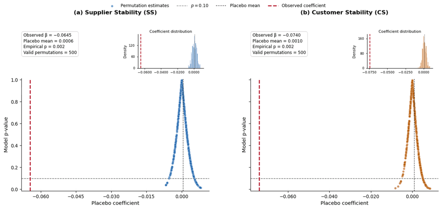
To examine whether the baseline estimates arise from accidental assignment or the industry–year composition of the sample, we conduct an industry–year stratified joint-permutation placebo test. In each iteration, supplier stability and customer stability are jointly permuted across firms within the same industry–year stratum. Joint permutation preserves the contemporaneous dependence between the two stability measures as well as their industry–year distributions, while breaking their firm-specific links with productivity. The remaining variables and panel identifiers are held unchanged. We then re-estimate the baseline two-way fixed-effects model with the full set of controls and firm-clustered standard errors. This procedure is repeated 500 times.

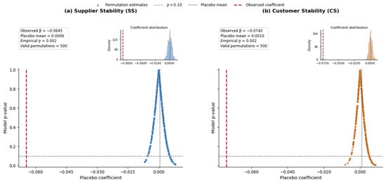
Figure 2 shows that the placebo coefficients are concentrated around zero. Their means are 0.0006 for supplier stability and 0.0010 for customer stability, whereas the corresponding observed coefficients are $-0.0645$ and $-0.0740$. Both observed estimates lie well outside the placebo distributions, and the permutation-based empirical p-values are 0.002. The results indicate that the negative baseline estimates are unlikely to be generated by random reassignment within the observed industry–year structure.

Figure 2. Industry–year stratified joint-permutation placebo test. Supplier stability and customer stability are jointly permuted within industry–year strata in each of 500 iterations. Each iteration re-estimates the baseline two-way fixed-effects model with firm-clustered standard errors. Colored points show permutation estimates, and small histograms above the main panels summarize their distributions. The red vertical lines denote the observed coefficients, the dotted vertical lines denote the means of the placebo distributions, and the horizontal dashed line indicates the 10% significance threshold.

7. Heterogeneity and Boundary Conditions

7.1. Heterogeneity by R&D Investment

Table 13 separates firms with and without positive R&D expenditure. The supplier-stability coefficient is more negative among firms without R&D investment ($-0.0669$) than among firms with positive R&D investment ($-0.0465$), and the SUEST test rejects coefficient equality at the 5% level ($p=0.0239$). The corresponding customer-stability coefficients are $-0.0729$ and $-0.0620$, with a marginally significant cross-group difference ($p=0.0893$). These results identify R&D investment as a boundary condition rather than a reversal of the baseline relationship. The weaker negative coefficients among firms undertaking R&D are consistent with greater absorptive and adaptive capacity, which may help them reconfigure production processes and reduce some of the rigidity associated with persistent partner portfolios. Nevertheless, both stability coefficients remain negative and significant in both groups.

Table 13. Heterogeneity analysis by R&D investment.

	(1)	(2)
Variable	No R&D Investment	Positive R&D Investment
$\mathit{SS}$	$-0.0669$ ***	$-0.0465$ ***
	$(-12.994)$	$(-2.887)$
$\mathit{CS}$	$-0.0729$ ***	$-0.0620$ ***
	$(-13.649)$	$(-3.898)$
Control variables	YES	YES
Firm fixed effects	YES	YES
Year fixed effects	YES	YES
Observations	384,930	58,576
Within $R^2$	$0.0468$	$0.1113$
SUEST p-value	$0.0239$ ** ($\mathit{SS}$)	$0.0893$ * ($\mathit{CS}$)

Notes: The final row reports two-sided p-values from formal SUEST cross-group coefficient-equality tests for supplier stability ($\mathit{SS}$) and customer stability ($\mathit{CS}$). Stars attached to these p-values indicate rejection of coefficient equality at the corresponding level. The table reports t-statistics in parentheses. Standard errors are clustered at the firm level. ***, ** and * indicate statistical significance at the 1%, 5%, and 10% levels, respectively.

7.2. Regional Heterogeneity

The regional results in Table 14 reveal distinct upstream and downstream boundary conditions. The supplier-stability coefficient is more negative in the central–western region ($-0.0719$) than in the eastern region ($-0.0640$), and the SUEST test strongly rejects coefficient equality ($p=0.0003$). This pattern is consistent with thinner supplier markets, higher rematching costs, and more limited alternative sourcing opportunities in central and western regions. By contrast, the customer-stability coefficient is more negative in the eastern region ($-0.0755$) than in the central–western region ($-0.0719$), with a significant cross-group difference ($p=0.0419$). In denser and more competitive eastern markets, retaining an established customer portfolio may impose greater opportunity costs by limiting the reallocation of sales toward emerging customers and market segments. Geography therefore conditions supplier-side and customer-side stability through different market environments, although both coefficients remain negative and significant in each regional subsample.

Table 14. Regional heterogeneity analysis.

	(1)	(2)
Variable	Central–Western Region	Eastern Region
$\mathit{SS}$	$-0.0719$ ***	$-0.0640$ ***
	$(-6.472)$	$(-13.004)$
$\mathit{CS}$	$-0.0719$ ***	$-0.0755$ ***
	$(-6.537)$	$(-14.911)$
Control variables	YES	YES
Firm fixed effects	YES	YES
Year fixed effects	YES	YES
Observations	83,820	359,686
Within $R^2$	$0.0634$	$0.0478$
SUEST p-value	$0.0003$ *** ($\mathit{SS}$)	$0.0419$ ** ($\mathit{CS}$)

Notes: The final row reports two-sided p-values from formal SUEST cross-group coefficient-equality tests for supplier stability ($\mathit{SS}$) and customer stability ($\mathit{CS}$). Stars attached to these p-values indicate rejection of coefficient equality at the corresponding level. The table reports t-statistics in parentheses. Standard errors are clustered at the firm level. ***, ** and * indicate statistical significance at the 1%, 5%, and 10% levels, respectively.

8. Discussion

8.1. Economic Interpretation of the Estimates

The fixed-effects estimates challenge the view that relationship continuity necessarily improves productive efficiency. Supplier and customer stability have significant negative coefficients after controlling for time-invariant firm heterogeneity, common annual shocks, and observed financial characteristics. The 2SLS estimates using leave-one-out same-industry peer stability as instruments remain negative, while the remaining validation exercises reproduce the same pattern. Taken together, the results indicate that dependence and rigidity embedded in persistent partner portfolios can outweigh their coordination benefits for SMEs, subject to the identifying qualifications discussed below.

The estimated magnitudes are also economically meaningful. Based on the preferred fixed-effects specification, a one-standard-deviation increase in supplier stability is associated with a 0.0171-log-point decrease in TFP, equivalent to an approximate 1.70% reduction. The corresponding estimate for customer stability is 0.0200 log points, or approximately 1.98%. These magnitudes indicate that persistent reliance on incumbent suppliers and customers has a nontrivial productivity implication for SMEs.

The channel results show how partner retention is related to different operating dimensions. Stable ties are associated with higher gross margins and total asset turnover, but also with greater expense burdens, lower operating margins, slower inventory turnover, and longer operating cycles. These patterns are consistent with coordination gains and relationship-adjustment burdens coexisting with the lower TFP estimates, although they are not interpreted as a formal decomposition of the total productivity effect.

The DomiRank interactions identify network dominance as an important boundary condition. Their positive coefficients show that the negative conditional coefficients in Equations (12) and (13) become smaller as network dominance increases. A stronger position makes outside options more credible, widens access to information, and reduces the disruption involved in rematching. Network dominance therefore appears to help SMEs retain valuable relationships while limiting the productivity costs associated with dependence.

The subgroup results identify two additional boundary conditions. Positive R&D investment weakens the negative relationships between partner retention and productivity, consistent with greater absorptive and adaptive capacity. Regional conditions operate asymmetrically across the supply chain: supplier retention is more negatively related to productivity in central and western regions, whereas customer retention is more negatively related to productivity in the eastern region. These findings show that the productivity implications of persistent relationships depend on both internal capabilities and the external market environment.

8.2. Measurement and Statistical Modeling Contributions

The first contribution extends the coverage and interpretation of longitudinal partner measurement. Earlier work has distinguished stability from concentration using disclosed major counterparties, including a transaction-share-weighted index among the top five [1]. Our invoice-based statistics instead measure the share of all observed current purchases or sales attributable to partners retained from the preceding year. This representation of interfirm exchange connects portfolio-wide persistence to the economic mechanisms of coordination, dependence, and hold-up [9,13,14,15].

Second, the study introduces a network-augmented statistical specification in which bilateral retention and global structural position enter the same productivity model. The interactions between DomiRank and the two retention measures capture how network position changes the productivity effects of partner persistence. The model thereby separates three objects that are often conflated: within-period partner concentration, between-period partner persistence, and the firm’s position in the full transaction network.

Third, the analysis combines large-scale relational data with panel econometrics. Firm and year fixed effects, firm-clustered inference, instrumental-variable estimation, matching, alternative measurements, high-dimensional fixed effects, and lagged specifications address different sources of uncertainty and provide a replicable modeling strategy for relating longitudinal transaction statistics and network measures to firm outcomes.

8.3. Implications for Mathematical Economics and Empirical Decision Support

From a mathematical-economics perspective, partner retention describes persistence in bilateral exchange, while DomiRank captures the structural alternatives available around the focal node. The interaction results show that the productivity effect of a local relationship statistic depends on the surrounding network. This finding provides empirical support for models in which outside options condition the costs of dependence and relationship-specific investment.

The measures also have a practical interpretation. Firms with sufficiently detailed transaction records can monitor value-weighted retention together with substitute availability, partner-specific assets, payment terms, inventory commitments, and switching costs. A high retention rate is less costly when credible alternatives remain accessible, but the same rate creates vulnerability when the firm occupies a weak network position. The framework therefore supports supplier and customer portfolio evaluation by jointly considering continuity and structural outside options.

SME managers should therefore treat partner retention as a portfolio decision rather than an unconditional objective: long-standing ties should be maintained when their coordination benefits exceed the accompanying dependence and switching costs. Firms occupying weaker network positions should periodically evaluate alternative suppliers and customers, payment terms, partner-specific investments, and inventory commitments, and use dual sourcing, customer diversification, modular operating arrangements, or contingency finance to preserve relational benefits without sacrificing strategic flexibility.

Policy and platform interventions can similarly focus on feasible alternatives rather than continuity alone. Reliable information about counterparties’ credit, quality, fulfillment, and demand conditions can reduce search and verification costs. Contract enforcement and accessible working-capital finance can limit the pressure created by delayed payment or asymmetric dependence. Such interventions can preserve valuable relationships while maintaining firms’ capacity to reorganize their portfolios.

8.4. Limitations and Future Research

The causal interpretation of the 2SLS estimates depends on the exclusion restriction for the peer stability instruments. Although the leave-one-out construction prevents a focal firm’s own stability from mechanically entering its instrument, contemporaneous industry-level conditions may affect both peer retention and firm productivity. Firm and year fixed effects and observed covariates reduce this concern but cannot eliminate every industry-specific time-varying channel. The IV results should therefore be interpreted conditional on the stated exclusion restriction. Future research could exploit policy changes or natural disruptions to obtain additional quasi-experimental variation and examine the operating channels more directly.

The analysis uses digitized transaction records as an observational source; it does not measure firms’ digital capabilities or technology adoption. Future research could link transaction networks to managerial use of transaction analytics or documented organizational changes. Longer panels could also distinguish short-lived adjustments from persistent changes in partner portfolios and permit richer analysis of temporal dependence.

Finally, the database cannot observe transactions outside its coverage, and invoices reveal neither contractual terms nor product quality, informal cooperation, or the value of partner-specific investment. DomiRank measures structural dominance rather than contractual bargaining or product-market power. The estimates generalize most directly to formal-sector Chinese SMEs observed in the VAT-invoice system during 2019–2025, a period that includes the COVID-19 disruption and subsequent recovery. China’s invoicing institutions, supply-chain organization, and SME financing environment may differ from those in other economies. The measurement framework may be informative in settings with broad electronic-invoicing coverage and similarly resource-constrained SMEs, but the estimated coefficient magnitudes should not be presumed universal. Linking invoices with contracts, payment histories, surveys, or product data and replicating the analysis in other periods and economies would clarify the mechanisms and scope of the findings.

9. Conclusions

This study constructs transaction-value-weighted longitudinal measures of supplier and customer retention and embeds them in a network-augmented panel model of SME productivity. Using 443,506 firm–year observations, the fixed-effects estimates show significant negative relationships between both retention measures and TFP. Two-stage least-squares estimates using leave-one-out same-industry peer stability as instruments are also negative under the corresponding identifying assumptions. Positive interactions with DomiRank show that network dominance attenuates these negative relationships.

The operating-channel evidence indicates a trade-off: higher gross margins and asset utilization coexist with greater expenses, lower operating profitability, slower inventory turnover, and longer operating cycles. The findings demonstrate that longitudinal partner statistics and network position describe distinct but complementary dimensions of interfirm organization. Their joint use provides a statistical and econometric basis for explaining productivity heterogeneity and evaluating supplier and customer portfolios among SMEs.

References

- Gu, J.; Shi, X.; Wang, P.; Xu, X. Examining the impact of upstream and downstream relationship stability and concentration on firms’ financial performance. J. Bus. Res. 2022, 141, 229–242. [Google Scholar] [CrossRef] [Scilit]
- Jiang, S.; Yeung, A.C.L.; Han, Z.; Huo, B. The Effect of Customer and Supplier Concentrations on Firm Resilience during the COVID-19 Pandemic: Resource Dependence and Power Balancing. J. Oper. Manag. 2023, 69, 497–518. [Google Scholar] [CrossRef] [Scilit]
- Liang, J. The Effect of Customer and Supplier Concentration on Firm Productivity: The Moderating Role of the Firm’s Dominant Position in the Supply Chain Network. Int. J. Prod. Econ. 2026, 297, 109727. [Google Scholar] [CrossRef] [Scilit]
- Diem, C.; Borsos, A.; Reisch, T.; Kertész, J.; Thurner, S. Quantifying Firm-Level Economic Systemic Risk from Nation-Wide Supply Networks. Sci. Rep. 2022, 12, 7719. [Google Scholar] [CrossRef] [Scilit] [PubMed]
- Bernard, A.B.; Moxnes, A.; Saito, Y.U. Production Networks, Geography, and Firm Performance. J. Political Econ. 2019, 127, 639–688. [Google Scholar] [CrossRef] [Scilit] [PubMed]
- Carvalho, V.M.; Nirei, M.; Saito, Y.U.; Tahbaz-Salehi, A. Supply Chain Disruptions: Evidence from the Great East Japan Earthquake. Q. J. Econ. 2021, 136, 1255–1321. [Google Scholar] [CrossRef] [Scilit]
- Morrissey, W.J.; Pittaway, L. Buyer–Supplier Relationships in Small Firms: The Use of Social Factors to Manage Relationships. Int. Small Bus. J. 2006, 24, 272–298. [Google Scholar] [CrossRef] [Scilit]
- Serpa, J.C.; Krishnan, H. The Impact of Supply Chains on Firm-Level Productivity. Manag. Sci. 2018, 64, 511–532. [Google Scholar] [CrossRef] [Scilit]
- Williamson, O.E. Transaction-Cost Economics: The Governance of Contractual Relations. J. Law Econ. 1979, 22, 233–261. [Google Scholar] [CrossRef] [Scilit]
- Dyer, J.H.; Singh, H. The Relational View: Cooperative Strategy and Sources of Interorganizational Competitive Advantage. Acad. Manag. Rev. 1998, 23, 660–679. [Google Scholar] [CrossRef] [Scilit]
- Krause, D.R.; Handfield, R.B.; Tyler, B.B. The relationships between supplier development, commitment, social capital accumulation and performance improvement. J. Oper. Manag. 2007, 25, 528–545. [Google Scholar] [CrossRef] [Scilit]
- Yang, J.; Wang, J.; Wong, C.W.; Lai, K.H. Relational stability and alliance performance in supply chain. Omega 2008, 36, 600–608. [Google Scholar] [CrossRef] [Scilit]
- Klein, B.; Crawford, R.G.; Alchian, A.A. Vertical Integration, Appropriable Rents, and the Competitive Contracting Process. J. Law Econ. 1978, 21, 297–326. [Google Scholar] [CrossRef] [Scilit]
- Grossman, S.J.; Hart, O.D. The Costs and Benefits of Ownership: A Theory of Vertical and Lateral Integration. J. Political Econ. 1986, 94, 691–719. [Google Scholar] [CrossRef] [Scilit] [PubMed]
- Pfeffer, J.; Salancik, G.R. The External Control of Organizations: A Resource Dependence Perspective; Harper & Row: New York, NY, USA, 1978. [Google Scholar]
- Bellamy, M.A.; Ghosh, S.; Hora, M. The influence of supply network structure on firm innovation. J. Oper. Manag. 2014, 32, 357–373. [Google Scholar] [CrossRef] [Scilit]
- Su, H.C.; Kao, T.W.D.; Linderman, K. Where in the Supply Chain Network Does ISO 9001 Improve Firm Productivity? Eur. J. Oper. Res. 2020, 283, 530–540. [Google Scholar] [CrossRef] [Scilit]
- Arora, S.; Brintrup, A. How Does the Position of Firms in the Supply Chain Affect Their Performance? An Empirical Study. Appl. Netw. Sci. 2021, 6, 19. [Google Scholar] [CrossRef] [Scilit]
- Engsig, M.; Tejedor, A.; Moreno, Y.; Foufoula-Georgiou, E.; Kasmi, C. DomiRank Centrality reveals structural fragility of complex networks via node dominance. Nat. Commun. 2024, 15, 56. [Google Scholar] [CrossRef] [Scilit] [PubMed]
- Levinsohn, J.; Petrin, A. Estimating Production Functions Using Inputs to Control for Unobservables. Rev. Econ. Stud. 2003, 70, 317–341. [Google Scholar] [CrossRef] [Scilit]
- Liu, J.; Wang, G. Supply chain stability and enterprises’ total factor productivity: From the perspective of development sustainability. Sustainability 2024, 16, 10265. [Google Scholar] [CrossRef] [Scilit]
- Delbufalo, E. Asset Specificity and Relationship Performance: A Meta-Analysis over Three Decades. J. Bus. Res. 2021, 134, 105–121. [Google Scholar] [CrossRef] [Scilit]
- Chen, M.; Tang, X.; Liu, H.; Gu, J. The Impact of Supply Chain Concentration on Integration and Business Performance. Int. J. Prod. Econ. 2023, 257, 108781. [Google Scholar] [CrossRef] [Scilit]
- David, T.; Troege, M.; Nguyen, H.M.; Nguyen, H.T. Relationship-Specific Investments for Up- and Downstream Firms and Credit Constraints. J. Corp. Financ. 2024, 84, 102534. [Google Scholar] [CrossRef] [Scilit]
- Han, Z.; Yu, C.; Li, Y. Customer Concentration and Supplier Financial Performance: An Inverted U-Shaped Relationship. Ind. Mark. Manag. 2023, 113, 138–152. [Google Scholar] [CrossRef] [Scilit]
- Gu, J.; Shi, X.; Wang, J.; Xu, X. Examining the Impact of Market Power Discrepancy between Supply Chain Partners on Firm Financial Performance. Int. J. Prod. Econ. 2024, 268, 109100. [Google Scholar] [CrossRef] [Scilit]
- Wang, T.; Deng, X.; Sheng, S.; Jia, Y. Mitigating the Damage of a Global Pandemic on the International Buyer–Supplier Relationship: Evidence from Chinese Suppliers. J. Bus. Res. 2024, 172, 114446. [Google Scholar] [CrossRef] [Scilit]
- Zhang, W.; Tao, Q.; Feng, Q.; Sun, Y. Supplier Concentration and Firm Risk-Taking: Transaction Cost Perspective. Econ. Model. 2024, 133, 106662. [Google Scholar] [CrossRef] [Scilit]
- Sharma, A.; Adhikary, A.; Borah, S.B.; Pathak, S. Supply Base Concentration and Firm Innovation Performance: A Contingency Study of Supply Base Breadth, Depth, Dispersion, and Collaboration. J. Bus. Res. 2024, 174, 114450. [Google Scholar] [CrossRef] [Scilit]
- Di, L.; Jiang, W.; Mao, J.; Zeng, Y. Managing Liquidity along the Supply Chain: Supplier-Base Concentration and Corporate Cash Policy. Eur. Financ. Manag. 2024, 30, 2376–2421. [Google Scholar] [CrossRef] [Scilit]
- Gelderman, C.J.; Semeijn, J.; Verhappen, M. Buyer Opportunism in Strategic Supplier Relationships: Triggers, Manifestations and Consequences. J. Purch. Supply Manag. 2020, 26, 100581. [Google Scholar] [CrossRef] [Scilit]
- Kwak, K.; Kim, N. Concentrate or Disperse? The Relationship between Major Customer Concentration and Supplier Profitability and the Moderating Role of Insider Ownership. J. Bus. Res. 2020, 109, 648–658. [Google Scholar] [CrossRef] [Scilit]
- Fabbri, D.; Klapper, L.F. Bargaining Power and Trade Credit. J. Corp. Financ. 2016, 41, 66–80. [Google Scholar] [CrossRef] [Scilit]
- Grewal, J.; Mohan, A.; Pérez-Cavazos, G. Payment Practices Transparency and Customer-Supplier Dynamics. J. Account. Res. 2024, 62, 635–674. [Google Scholar] [CrossRef] [Scilit]
- Du, C.; Zhang, Q. Supply Network Position, Digital Transformation and Innovation Performance: Evidence from Listed Chinese Manufacturing Firms. PLoS ONE 2022, 17, e0279133. [Google Scholar] [CrossRef] [Scilit] [PubMed]
- Fan, X.; Gao, Y.; Wang, J. Does Supply Chain Network Location Affect Innovation Performance of Manufacturing Enterprises? Evidence from China. Systems 2025, 13, 767. [Google Scholar] [CrossRef] [Scilit]
- Lavassani, K.M.; Movahedi, B. Firm-Level Analysis of Global Supply Chain Network: Role of Centrality on Firm’s Performance. Int. J. Glob. Bus. Compet. 2021, 16, 86–103. [Google Scholar] [CrossRef] [Scilit]
- Nezami, M.; Chisam, N.; Palmatier, R.W. Network Centrality and Firm Performance: A Meta-Analysis. J. Acad. Mark. Sci. 2025, 53, 79–104. [Google Scholar] [CrossRef] [Scilit]
- Dong, Y.; Skowronski, K.; Song, S.; Venkataraman, S.; Zou, F. Supply Base Innovation and Firm Financial Performance. J. Oper. Manag. 2020, 66, 768–796. [Google Scholar] [CrossRef] [Scilit]
- Borgatti, S.P.; Li, X. On Social Network Analysis in a Supply Chain Context. J. Supply Chain. Manag. 2009, 45, 5–22. [Google Scholar] [CrossRef] [Scilit]
- Kim, Y.; Chen, Y.S.; Linderman, K. Supply Network Disruption and Resilience: A Network Structural Perspective. J. Oper. Manag. 2015, 33–34, 43–59. [Google Scholar] [CrossRef] [Scilit]
- Solow, R.M. Technical Change and the Aggregate Production Function. Rev. Econ. Stat. 1957, 39, 312–320. [Google Scholar] [CrossRef] [Scilit]
- Syverson, C. What Determines Productivity? J. Econ. Lit. 2011, 49, 326–365. [Google Scholar] [CrossRef] [Scilit]
- Hsieh, C.T.; Klenow, P.J. Misallocation and Manufacturing TFP in China and India. Q. J. Econ. 2009, 124, 1403–1448. [Google Scholar] [CrossRef] [Scilit]
- Xu, H.; Li, Y.; Lin, W.; Wang, H. ESG and Customer Stability: A Perspective Based on External and Internal Supervision and Reputation Mechanisms. Humanit. Soc. Sci. Commun. 2024, 11, 981. [Google Scholar] [CrossRef] [Scilit]
- Borgatti, S.P. Centrality and Network Flow. Soc. Netw. 2005, 27, 55–71. [Google Scholar] [CrossRef] [Scilit]
- Brin, S.; Page, L. The Anatomy of a Large-Scale Hypertextual Web Search Engine. Comput. Netw. Isdn Syst. 1998, 30, 107–117. [Google Scholar] [CrossRef] [Scilit]
- Gleich, D.F. PageRank Beyond the Web. SIAM Rev. 2015, 57, 321–363. [Google Scholar] [CrossRef] [Scilit]
- Coad, A.; Segarra, A.; Teruel, M. Like Milk or Wine: Does Firm Performance Improve with Age? Struct. Change Econ. Dyn. 2013, 24, 173–189. [Google Scholar] [CrossRef] [Scilit]
- Coricelli, F.; Driffield, N.; Pal, S.; Roland, I. When Does Leverage Hurt Productivity Growth? A Firm-Level Analysis. J. Int. Money Financ. 2012, 31, 1674–1694. [Google Scholar] [CrossRef] [Scilit]
- Djankov, S.; Ganser, T.; McLiesh, C.; Ramalho, R.; Shleifer, A. The Effect of Corporate Taxes on Investment and Entrepreneurship. Am. Econ. J. Macroecon. 2010, 2, 31–64. [Google Scholar] [CrossRef] [Scilit]
- Doraszelski, U.; Jaumandreu, J. R&D and Productivity: Estimating Endogenous Productivity. Rev. Econ. Stud. 2013, 80, 1338–1383. [Google Scholar] [CrossRef] [Scilit]
- Nickell, S.J. Competition and Corporate Performance. J. Political Econ. 1996, 104, 724–746. [Google Scholar] [CrossRef] [Scilit]
- Aghion, P.; Bloom, N.; Blundell, R.; Griffith, R.; Howitt, P. Competition and Innovation: An Inverted-U Relationship. Q. J. Econ. 2005, 120, 701–728. [Google Scholar] [CrossRef] [Scilit]
- Geng, Y.; Wang, Y.; Wu, S. Acquaintance Means Booster? Why Stable Customers Matter for Firm Productivity. China J. Account. Res. 2025, 18, 100435. [Google Scholar] [CrossRef] [Scilit]
- Angrist, J.D.; Krueger, A.B. Instrumental Variables and the Search for Identification: From Supply and Demand to Natural Experiments. J. Econ. Perspect. 2001, 15, 69–85. [Google Scholar] [CrossRef] [Scilit]
- Jiang, T. Mediating and Moderating Effects in Empirical Studies of Causal Inference. China Ind. Econ. 2022, No. 5, 100–120. (In Chinese) [Google Scholar] [CrossRef]
- Baik, B.; Chae, J.; Choi, S.; Farber, D.B. Changes in Operational Efficiency and Firm Performance: A Frontier Analysis Approach. Contemp. Account. Res. 2013, 30, 996–1026. [Google Scholar] [CrossRef] [Scilit]
- Demeter, K.; Matyusz, Z. The Impact of Lean Practices on Inventory Turnover. Int. J. Prod. Econ. 2011, 133, 154–163. [Google Scholar] [CrossRef] [Scilit]
- Wang, Y.; Ji, Y.; Chen, X.; Song, C. Inflation, Operating Cycle, and Cash Holdings. China J. Account. Res. 2014, 7, 263–276. [Google Scholar] [CrossRef] [Scilit]
- Ackerberg, D.A.; Caves, K.; Frazer, G. Identification Properties of Recent Production Function Estimators. Econometrica 2015, 83, 2411–2451. [Google Scholar] [CrossRef] [Scilit]
Disclaimer/Publisher’s Note: The statements, opinions and data contained in all publications are solely those of the individual author(s) and contributor(s) and not of MDPI and/or the editor(s). MDPI and/or the editor(s) disclaim responsibility for any injury to people or property resulting from any ideas, methods, instructions or products referred to in the content. |
© 2026 by the authors. Licensee MDPI, Basel, Switzerland. This article is an open access article distributed under the terms and conditions of the Creative Commons Attribution (CC BY) license.