Fast Probabilistic Wind Power Forecasting via One-Step Consistency Distillation and Memory-Efficient CRPS Optimization

Abstract

Grid operators scheduling wind power act on the width of the predicted distribution, and diffusion-based forecasters have reported strong accuracy on wind benchmarks. That accuracy can come from a sampling chain of a hundred or more evaluations per member, with reported implementations incurring multi-second latency per farm against a dispatch cycle of minutes, while a one-step student distilled from such a chain can concentrate its members into a spread narrower than its own error. This paper introduces Consist-Wind, a one-step probabilistic wind power forecaster. A frozen point backbone supplies the conditioning context; a teacher diffusion model on numerical weather prediction (NWP) residuals is distilled into a one-step consistency student, one function evaluation per member, and a stabilized shifted-logit warp maps generated members to the physical power range. A fourth phase calibrates the student by training its ensemble against the continuous ranked probability score (CRPS), which recovers the spread and raises the accuracy of the one-step forecast. Evaluated at every update, its pairwise form governs the training footprint, so the sorted-rank form of the CRPS is used, quasilinear in time and linear in memory. The cost of calibration is decoupled from the ensemble width by a scalable ensemble calibration principle, with the objective on order statistics and query-chunked attention (QCA) inside the kernel launch limit, so the whole pipeline trains and runs on a single device with limited compute. In our experiments on GEFCom2014-W, SDWPF, and GEFCom2012-W, Consist-Wind achieves the lowest CRPS, 3.1% below the strongest reproduced baseline, reduces the calibration error of the distilled student by 45%, issues a forecast in 0.03 ms for a speedup of about 66× relative to the reproduced multi-step reference, and reduces the memory required to evaluate the pairwise penalty term by 98%, admitting 500-member calibration ensembles on the evaluation device. Distributional forecasts of this accuracy, trained within a limited-compute budget, bring uncertainty-aware scheduling within reach of operators on commodity hardware.

1. Introduction

Probabilistic wind power forecasting has become an essential tool for grid operators, who use the width of the predicted distribution to size reserve capacity and plan dispatch ahead of ramps [1,2]. The continuous ranked probability score (CRPS), established by the GEFCom competitions, is the standard metric for such forecasts [2,3].

A long line of work has been devoted to this task. Early forecasters obtain the predictive distribution from quantile regression [4], adaptive statistical and forecast-combination methods [1], or parametric families such as DeepAR and the temporal fusion transformer [5,6], which use a fixed parametric output family (with autoregressive rollout where applicable). Deep generative models go further by learning the shape of the distribution itself: normalizing flows map a base distribution through invertible transformations [7], and diffusion models refine a noise sample through a learned denoising chain [8,9,10], with strong CRPS results reported on their respective wind-power benchmarks.

Diffusion models pay for this accuracy with a long sampling chain: generating one ensemble member can require a hundred or more denoising steps, incurring multi-second latency per wind farm in reported implementations, while a dispatch cycle closes in a few minutes [8,9]. Distilling such a model into a one-step consistency student reduces each member to a single network evaluation [11,12,13], and the student can issue ensembles that are too narrow because the intermediate steps of the chain, which a multi-step sampler uses to separate its samples, are removed [14]. Training the student against CRPS restores the spread [11,13,15,16], and the standard estimator compares every pair of members, materializing an $(N,H,K,K)$ tensor at every update, a bandwidth-bound cost that grows quadratically with the ensemble size and saturates the memory of the device before the network does. The activations of the network compete for the same memory, and multi-scale patching pushes the attention batch dimension past the fused-kernel launch limit. These implementation-level loads are analyzed in the complexity and systems sections; the scoring-rule references establish the statistical objective and finite-ensemble correction.

Consist-Wind is proposed as a one-step probabilistic wind power forecaster for these problems. A deterministic point forecast backbone is trained and frozen, providing the conditioning context for all later stages. A teacher diffusion model is trained on the residuals between the observed power and the point forecast, and is distilled into a one-step consistency student, so that each ensemble member is generated with a single function evaluation, which removes the sampling cost. A stabilized shifted-logit warp maps every member to the physical power range and preserves the shape of the distribution within the stabilized coordinate. The student is then calibrated by training its ensemble against CRPS, which recovers the spread lost in distillation and raises the accuracy of the one-step forecast. Calibration quality grows with the ensemble width, so the cost of calibration is decoupled from that width by two method-level restructurings under a scalable ensemble calibration principle: the objective runs on the order statistics of the ensemble in linear memory, and the attention of the long-horizon backbone runs as query-chunked attention (QCA) within the fused-kernel launch limit; training runs in half precision with gradient checkpointing. The whole method therefore trains and runs on a limited-compute device.

In our experiments on GEFCom2014-W, SDWPF, and GEFCom2012-W, Consist-Wind achieves the lowest CRPS, 3.1% below the strongest reproduced baseline, generates a forecast in 0.03 ms, a speedup of about 66× relative to the reproduced multi-step reference, reduces the calibration error of the distilled student by 45%, and reduces the memory required to evaluate the pairwise penalty term by 98%, admitting 500-member calibration ensembles on the evaluation device. Ablations attribute the accuracy gain to the calibration phase and the memory gain to the sorted-rank objective, which trains at an identical score.

The main contributions of this work are summarized as follows:

• Consist-Wind, a one-step probabilistic wind power forecaster obtained by distilling a residual diffusion teacher into a consistency student, in which each ensemble member costs a single function evaluation and a stabilized shifted-logit warp maps the members to the physical power range.
• A calibration phase that trains the student against CRPS, recovering the spread lost in distillation and raising the accuracy of the one-step forecast.
• Scalable ensemble calibration, realized by two method-level restructurings. The calibration quality of the one-step forecaster grows with the ensemble width, and each restructuring removes one bottleneck between that width and a single-device budget. The calibration objective replaces bandwidth-bound $O\left(K^2\right)$ tensor materialization with $O\left(K\log K\right)$ order-statistic computation, so the cost of scoring an ensemble grows quasilinearly in its width. The attention of the patched backbone runs as query-chunked attention (QCA), which decomposes the attention batch dimension into independent subproblems that each fit the fused-kernel launch limit and couples them through a low-rank global context. Together, the two restructurings cut the memory of the training objective by an order of magnitude, raise the calibration ensemble ceiling to several times the pairwise limit on a consumer GPU, and keep long-horizon attention within the kernel launch limit, all at an identical score.
• Validation on GEFCom2014-W, SDWPF, and GEFCom2012-W, with ablations that attribute the accuracy, calibration, speed, and memory effects to their respective components.

2. Related Work

2.1. Probabilistic Wind Power Forecasting

The GEFCom competitions established CRPS and the pinball loss as the standard metrics of probabilistic energy forecasting [2,3]. Early forecasters obtained the predictive distribution from quantile regression [4], adaptive statistical and forecast-combination methods [1], or parametric families such as DeepAR and the temporal fusion transformer [5,6]. These models use a fixed parametric output family (with autoregressive rollout where applicable), and deep generative models have since reported lower CRPS on their respective benchmarks by learning the shape of the distribution itself, beginning with normalizing flows [7] and continuing through diffusion forecasters [8,9,10,17], NWP-bias-correction models [18], dual-exogenous-variable transformers [19], and BERT-based sequence models [20]. Several diffusion studies report strong CRPS in this set of work, but their datasets and evaluation settings are not directly comparable; their iterative refinement can incur multi-second latency for one wind farm in reported implementations [9], while competition solutions on SDWPF operate under budgets of milliseconds [21]. Graph models [22,23] and spatiotemporal transformers [24,25,26,27] raise point accuracy through the conditioning path and retain the probabilistic head they are given, so the evaluations per member and the memory of the ensemble score remain properties of that head. The present work keeps the accuracy of the diffusion route and moves both quantities, sampling to one evaluation per member and the score to memory linear in the ensemble, and its CRPS calibration lowers the score further, below the diffusion teacher, so that the one-step forecaster is more accurate as well as faster.

2.2. Fast Sampling for Diffusion Models

Consistency models distil a diffusion teacher into a network mapping any point of a probability flow trajectory to its endpoint, so one function evaluation yields a sample [11]. Latent consistency models extend this to latent diffusion with classifier-free guidance [12], SWIFT transfers it to time series [13], and efficient wind forecasters also combine graph and WaveNet components [28]. Progressive distillation [29] and DDIM [30] take fewer and larger steps along the same trajectory and spend several evaluations per sample. The distillation objective aligns the student pointwise to the teacher trajectory, and the intermediate steps of that trajectory are what a multi-step sampler uses to separate its samples, so a one-step student can produce a narrow and overconfident ensemble, an effect attributed to the covariate shift between the noise levels seen during distillation and at inference [14]. Image synthesis judges the individual sample. The width of the ensemble is the forecast product in wind power, which makes the spread of the student a quantity the training pipeline has to restore, and fine-tuning against a proper scoring rule is the established route [11]. Two further properties are specific to this domain, since the target lies in $[0,1]$ and the sampler ranges over the real line, and the quantity worth modelling generatively is the NWP residual. In Consist-Wind, the consistency step therefore carries a bounded-power warp and a calibration phase whose objective runs at the ensemble sizes that calibration requires.

2.3. Cost of Training on a Proper Scoring Rule

CRPS is a strictly proper scoring rule, minimized uniquely by the true predictive distribution [15], which is what allows it to serve as a training objective, and a forecaster trained on it evaluates it at every parameter update. The standard ensemble estimator is the pairwise energy form [15], whose cost scales quadratically with ensemble size, and every later refinement keeps that structure, including the fair adjustment for finite-ensemble bias [31] and the weighted [32], threshold-weighted [33], and multi-scale [16] extensions to tails and spatial structure. The pairwise tensor is stored for every horizon step of every batch element, so memory decides the largest ensemble that gradients flow through, and spread is a property the loss reads from that ensemble. Limited-information CRPS estimators trade exactness for estimation cost [34]; extreme-event subset evaluation can introduce selection effects [35], whereas the Energy Score report discusses discrimination and sampling issues for multivariate forecasts [36]. Sorted-rank and probability-weighted-moment forms of the ensemble CRPS compute the same empirical quantity in quasilinear time with memory linear in the ensemble size [37,38,39]; the sorted-rank form provides the differentiable scoring expression used for calibration and evaluation.

Gradient checkpointing is a standard technique that reduces the memory of the network layers [40]; training runs in half precision throughout. The tensor that dominates the memory of an ensemble forecaster lives in the loss. Efficiency work on renewable forecasting has concentrated on model compression [41] and federated learning [42], which shrink the network or distribute it across devices. The cost of calibration is decoupled from the ensemble width under a scalable ensemble calibration principle: the objective it optimizes during training is computed on the order statistics of the ensemble in linear memory, and the attention of the backbone runs as query-chunked attention (QCA) within the fused-kernel launch limit, with the chunks coupled through a low-rank global context. Consist-Wind therefore combines single-evaluation sampling, a sorted-rank CRPS objective with linear memory, and a bounded-power guarantee.

3. Method

3.1. Overview

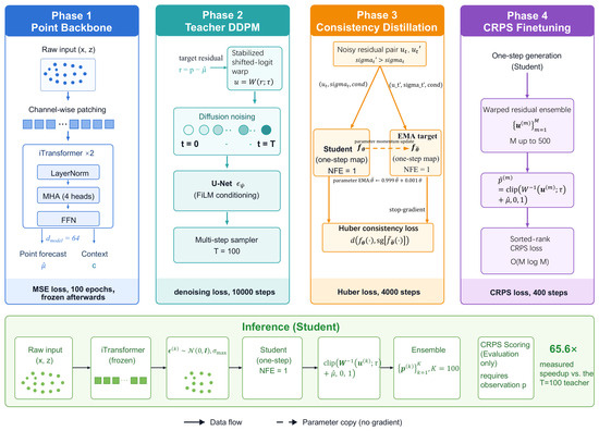
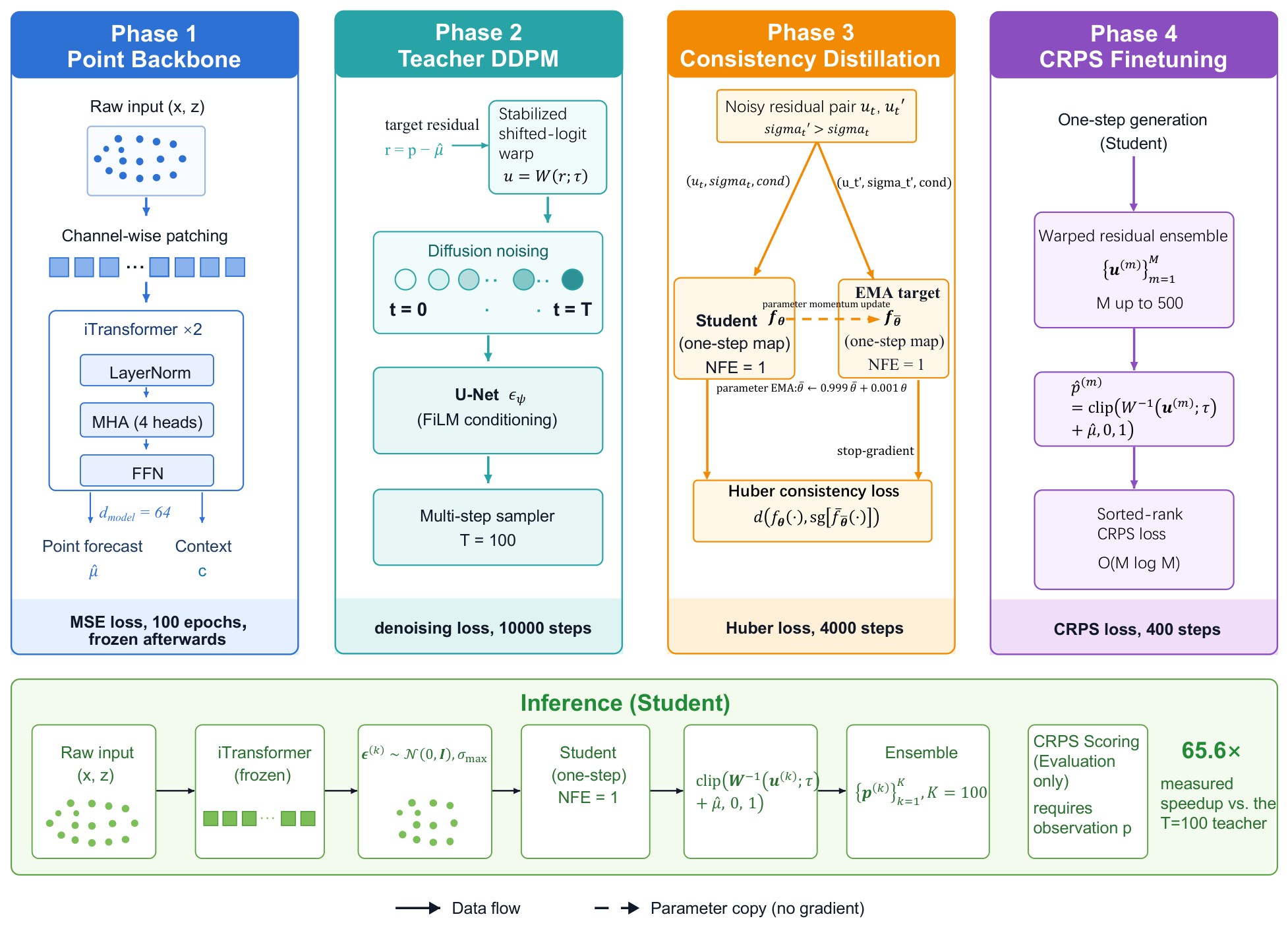
Consist-Wind is a one-step conditional generator of wind power ensembles, built in four training phases and deployed as a single network evaluation per member. Figure 1 shows the complete flow. In the first phase, a deterministic point forecast backbone is fitted on the observed power and then frozen, providing a point forecast and a context embedding for all later stages. In the second phase, the diffusion model [8,9] is extended to the warped residual, so the boundary mass of the power range stays finite. In the third phase, a one-step consistency student [11] is distilled on the warped residual, so it operates in the same coordinate as the teacher. The distilled student is fast, and its ensemble is under-dispersed, so the fourth phase calibrates it by training its ensemble against CRPS, which makes the score an internal objective of the forecaster. The CRPS, in its classical sorted-rank form [37,38,39], is used with the finite-ensemble correction, keeping the objective’s memory linear in the ensemble size.

Figure 1. Consist-Wind’s four-phase training pipeline and one-step deployment path. Phase 1 trains a deterministic iTransformer backbone ($d_{\mathrm{model}}=64$, two layers, four-head attention) and freezes it; this backbone provides both point prediction $\widehat{\mu }$ and context embedding c for all subsequent phases. Phase 2 trains a teacher diffusion model on the transformed residual $u=W\left(r\right)$, where W is the stabilized shifted-logit coordinate defined in the text. Phase 3 distills the teacher into a one-step consistency student via trajectory self-consistency, reducing sampling from $T\sim 100$ network evaluations per member to exactly one. Phase 4 calibrates the student ensemble by training its collective with CRPS, recovering the ensemble spread lost in distillation. At deployment, a single forward pass through the student produces K residual members in parallel; the stabilized inverse transform $W^{-1}$ and the point forecast $\widehat{\mu }$ map them back to physical power, yielding a calibrated probabilistic forecast.

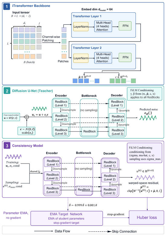
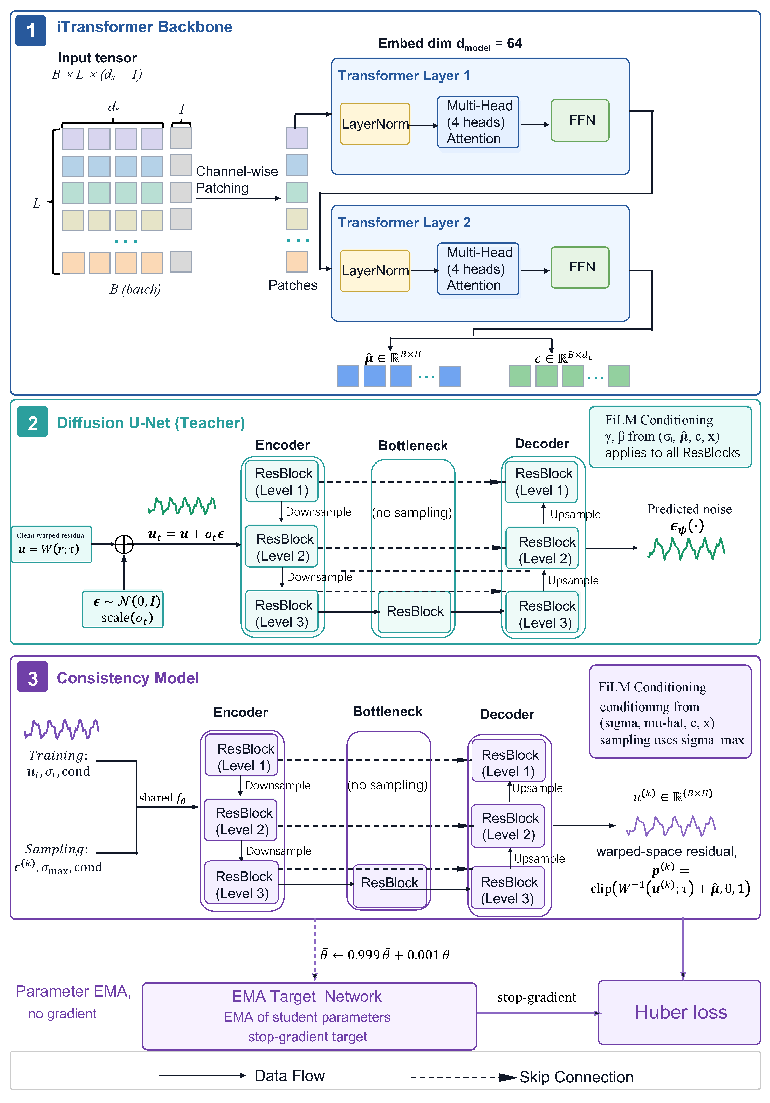
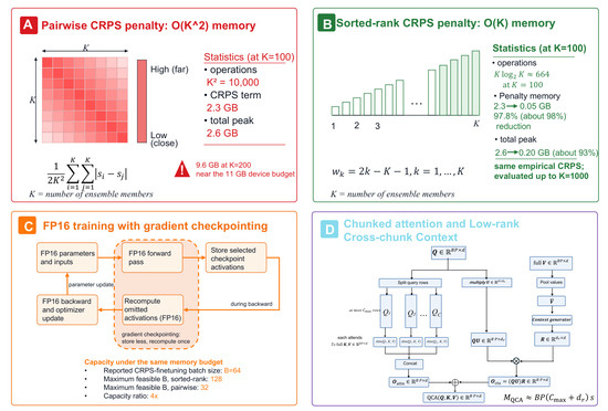
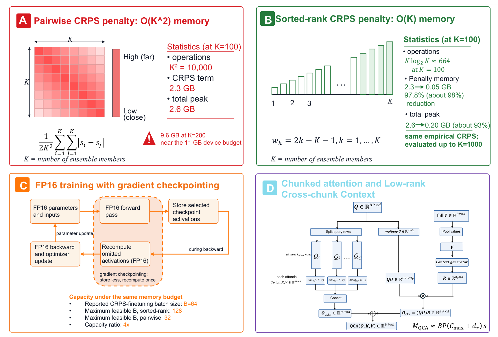
Two design choices keep the four phases within a limited compute budget, realised under the scalable ensemble calibration principle: the calibration objective runs on the order statistics of the ensemble in linear memory, attention runs as query-chunked attention (QCA) within the kernel launch limit, and training runs in half precision with gradient checkpointing as the standard configuration. The backbone attention [43] extends this chunked form with a low-rank cross-chunk context term, which retains the global information. Figure 2 details the three network components, and Figure 3 summarizes the restructurings that keep training and deployment within limited compute.

Figure 2. Network internals for the three trained components. (1) iTransformer backbone: channel-wise tokenization feeds two transformer layers (four heads, $d_{\mathrm{model}}=64$) that emit the point forecast $\widehat{\mu }\in {\mathbb{R}}^{B\times H}$ and the context embedding c, where H is the forecast horizon. Trained once with an MSE objective and frozen thereafter. (2) Teacher diffusion U-Net: a three-level encoder–decoder over the noised transformed residual $u_t=u+{\sigma }_t\epsilon$, with skip connections and FiLM conditioning [44] that modulates the residual blocks using the noise level ${\sigma }_t$ together with $\widehat{\mu }$, c and x. (3) Consistency model: the same U-Net topology, trained across paired noise levels by the Huber consistency objective. At sampling time it is evaluated once at the fixed noise level ${\sigma }_{\max }$ and predicts $u_0$ directly rather than the noise residual. Each forward pass produces one ensemble member $u^{\left(k\right)}$ in the warped space, which must pass through $W^{-1}$ before it can be read as physical power. The EMA target supplies the distillation reference: it is a running average of the student parameters and provides the stop-gradient target for distillation. Phase 4 applies the CRPS objective to this student network; the training-level view is presented in Figure 1.

Figure 3. The scalable ensemble calibration restructurings that let Consist-Wind train and deploy on one consumer GPU. (A,B) restructure the objective arithmetic. The standard pairwise estimator materialises every member-to-member difference as an $(N,H,K,K)$ tensor, which at $K=100$ reaches 2.3 GB of the 2.6 GB total and approaches the 11 GB budget at about $K=200$. The sorted-rank form of the CRPS computes the identical quantity from the order statistics alone, cutting the penalty term to 0.05 GB, a 98% reduction in the memory required by the penalty computation that lifts the ensemble ceiling to $K=1000$, and cuts the arithmetic from quadratic to quasilinear. Because the pairwise form must build the full tensor before reducing it, the saving is bandwidth-bound: the arithmetic intensity grows from $O\left(1\right)$ to $O\left(\log K\right)$ in the ensemble size. (C) shows the standard training configuration: all computation runs in FP16, and gradient checkpointing trades stored activations for recomputation. (D) restructures the attention kernel: query-chunked attention (QCA) keeps long-horizon batches inside the fused-attention kernel launch limit by processing the query dimension in chunks, and a low-rank cross-chunk context term couples the chunks through a compact global summary. The sorted-rank CRPS is used in Phase 4 of Figure 1; checkpointing is a training configuration, while QCA is used by the point backbone in Phase 1 and when that backbone is evaluated at deployment. Measured costs are reported in Section 5.5.

3.2. Problem Setting and Notation

Let $x\in {\mathbb{R}}^{L\times d_x}$ denote the NWP covariates, wind speed, direction, and temperature, over a lookback window of L steps, $z\in {\mathbb{R}}^{L\times 1}$ the historical power observations, and $p\in {[0,1]}^H$ the per-unit power target over a forecast horizon of H steps. The deterministic backbone $g_{\varphi }$ produces the point forecast $\widehat{\mu }=g_{\varphi }(x,z)$. The probabilistic part of the model describes the residual $r=p-\widehat{\mu }$, which concentrates the uncertainty that NWP-based point forecasts leave behind. Because wind power is bounded, the residual is mapped through a stabilized shifted-logit warp W into an unbounded space before it is modelled, and the stabilized inverse maps the generated samples back at decoding. An ensemble forecast is a set of K members ${\left\{p^{\left(k\right)}\right\}}_{k=1}^K$ generated by the model for the same input, and it is scored against the observed p with CRPS. Table 1 summarizes the notation used throughout the paper.

Table 1. Notation summary.

Symbol	Description
$x\in {\mathbb{R}}^{L\times d_x}$	NWP covariates for wind speed, direction, temperature
$z\in {\mathbb{R}}^{L\times 1}$	Historical power observations over lookback L
$p\in {[0,1]}^H$	Target power in per-unit over horizon H
L	Lookback window in time steps
H	Forecast horizon in time steps
h	Forecast horizon in hours, $h=H\mathsf{\Delta }t$, with $\mathsf{\Delta }t$ the dataset time step (Section 4.1)
$g_{\varphi }$	Deterministic point forecast backbone, iTransformer
$\widehat{\mu }=g_{\varphi }(x,z)$	Point forecast
$r=p-\widehat{\mu }$	Residual of the NWP correction
$W,W^{-1}$	Shifted-logit power warp and stabilized inverse
q	Clipped unit-interval coordinate in the warp
${ϵ}_{\mathrm{clip}}$	Numerical clipping constant for q
$\tau$	Warp temperature
$u=W\left(r\right)$	Warped residual in unbounded space
c	Context embedding from the point-forecast backbone
$\mathrm{cond}$	Conditioning tuple $(\widehat{\mu },c,x)$
$f_{\theta }$	One-step consistency model
$\psi ,\overline{\theta }$	Teacher parameters and EMA student parameters
$\epsilon$	Standard Gaussian diffusion noise
$t,t^{\prime }$	Sampled noise-level indices
${\sigma }_t$	Noise scale at level t
$d(·,·),\delta$	Huber distance and transition parameter
${\left\{p^{\left(k\right)}\right\}}_{k=1}^K$	Ensemble forecast with K members
$s_{\left(k\right)}$	k-th order statistic of the sorted ensemble
M	Training calibration ensemble size
N	Number of windows in a calibration batch
P	Number of temporal patches
$C,C_{\max }$	Number and maximum width of query chunks
$d,d_r$	Attention width and low-rank context dimension
s	Bytes per stored numerical element
$W_{\mathrm{sort}}$	Width of the sorting workspace in the sorted-rank CRPS objective
T	Number of denoising steps in teacher DDPM
$\mathrm{NFE}$	Number of function evaluations per ensemble member
B	Batch size
${\sigma }_{\min },{\sigma }_{\max }$	Noise schedule bounds
↓	indicates that lower values of the metric correspond to better forecast performance.

3.3. Network Components

Point forecast backbone. The iTransformer architecture [43] is used, which tokenizes each input channel independently and applies self-attention across channels. Given the concatenated input $[x;z]$, the backbone outputs the point forecast $\widehat{\mu }$ and a context embedding c that condenses the input history. The backbone is trained once with a mean squared error objective and frozen afterwards, so its cost is paid exactly once.

Bounded-power warping. Wind power takes values in $[0,1]$, and the mass at the boundaries, calm and curtailment at zero and rated capacity at one, matters for reserve sizing. The residual $r=p-\widehat{\mu }$ lies in $[-1,1]$. We first map it to a numerically stable unit-interval coordinate and then apply a shifted logit coordinate,

$$\begin{array}{cccc}\hfill q& =\mathrm{clip}\left({\displaystyle \frac{r+1}{2}},{ϵ}_{\mathrm{clip}},1-{ϵ}_{\mathrm{clip}}\right),\hfill & \hfill u& =W(r;\tau )={\displaystyle \frac{1}{\tau }}\log {\displaystyle \frac{q}{1-q}},\hfill \\ \hfill r& =W^{-1}(u;\tau )=2\sigma \left(\tau u\right)-1,\hfill & \hfill & \hfill \end{array}$$

(1)

where ${ϵ}_{\mathrm{clip}}$ is a small numerical constant that keeps q in the open unit interval and $\sigma (·)$ is the logistic sigmoid. The displayed inverse applies to the interior of the stabilized coordinate; decoding applies the same stabilized inverse and then clips the reconstructed power to $[0,1]$. A generated member $u^{\left(k\right)}$ therefore produces $p^{\left(k\right)}=\mathrm{clip}(W^{-1}(u^{\left(k\right)};\tau )+\widehat{\mu },0,1)$.

Generative architecture. The teacher and the student share a U-Net-style temporal network with residual blocks and time embeddings. The conditioning input concatenates the point forecast $\widehat{\mu }$, the context embedding c, and the NWP features x, injected through feature-wise affine modulation of the residual blocks [44]. The teacher sees the whole range of noise levels and predicts the noise component; the student is evaluated at a single fixed noise level and predicts the denoised residual.

3.4. One-Step Consistency Distillation

Teacher diffusion. The teacher is fitted on the warped residuals $u=W\left(r\right)$ with the standard denoising objective [45],

$${\mathcal{L}}_{\mathrm{teacher}}={\mathbb{E}}_{u,\epsilon ,t}\left[\parallel \epsilon -{\epsilon }_{\psi }(u_t,{\sigma }_t,\mathrm{cond}){\parallel }^2\right],$$

(2)

where $u_t=u+{\sigma }_t\epsilon$, $\epsilon \sim \mathcal{N}(0,I)$, t indexes a sampled noise level, and ${\sigma }_t$ is sampled from the exponential schedule between ${\sigma }_{\min }$ and ${\sigma }_{\max }$. The symbol $\psi$ denotes the teacher parameters, and $\mathrm{cond}=(\widehat{\mu },c,x)$ denotes the conditioning variables. The teacher provides the denoising trajectories used by phase 3.

Consistency distillation. Consistency models enforce that any two noisy versions of the same clean sample map to the same output, so that the student learns the fixed point of the teacher’s probability flow [11]. The student $f_{\theta }$ is trained with the consistency loss

$${\mathcal{L}}_{\mathrm{CM}}={\mathbb{E}}_{u,t,t^{\prime }}\left[d\left(f_{\theta }(u_t,{\sigma }_t,\mathrm{cond}),\mathrm{sg}\left[f_{\overline{\theta }}(u_{t^{\prime }},{\sigma }_{t^{\prime }},\mathrm{cond})\right]\right)\right],$$

(3)

where t and $t^{\prime }$ index two noise levels with ${\sigma }_{t^{\prime }}>{\sigma }_t$, $\mathrm{sg}(·)$ stops the gradient, $d(·,·)$ is the Huber distance with transition parameter $\delta$, and $\overline{\theta }$ is the exponential moving average of the student parameters. After distillation, a member is generated as $\widehat{u}=f_{\theta }(\epsilon ,{\sigma }_{\max },\mathrm{cond})$ with $\epsilon \sim \mathcal{N}(0,I)$, using one forward pass.

3.5. Exact Sorted-Rank Form of the Calibration Objective

CRPS is a strictly proper scoring rule, minimized uniquely by the true predictive distribution [15], and inside Consist-Wind it serves as the loss of phase 4. It is evaluated at every update of that phase over the M members drawn for each batch, so its cost is a training cost, and on a small GPU it decides how many members the student is calibrated against.

Standard pairwise form. At one forecast coordinate, let ${\left\{s_k\right\}}_{k=1}^K$ be the ensemble members and let y be the corresponding observation. The empirical CRPS is

$$\mathrm{CRPS}(y,\left\{s_k\right\})={\displaystyle \frac{1}{K}}{\displaystyle \sum _{k=1}^K}|y-s_k|-{\displaystyle \frac{1}{2K^2}}{\displaystyle \sum _{i,j=1}^K}|s_i-s_j|.$$

(4)

The second term compares every pair of members. Computing it for K members and H time steps requires a $K\times K$ comparison matrix per time step, so the memory grows with the square of the ensemble size and saturates a small GPU long before the network does. The term also carries the gradients of the loss, which adds to the backward pass, so the objective sets the ceiling on the batch size and on the members that can be drawn for the loss.

Sorted-rank identity. The pairwise term can be replaced by an identity over the order statistics of the ensemble, a classical result of order-statistics theory used in the probabilistic-forecasting literature [37,38,39].

Let $s_{\left(1\right)}\le s_{\left(2\right)}\le \cdots \le s_{\left(K\right)}$ denote the order statistics of ${\left\{s_k\right\}}_{k=1}^K$. The pairwise term is written directly as

$${\displaystyle \sum _{i,j=1}^K}|s_i-s_j|=2{\displaystyle \sum _{k=1}^K}(2k-K-1)s_{\left(k\right)}.$$

(5)

Fast estimator. The fast estimator follows directly:

$${\mathrm{CRPS}}_{\mathrm{fast}}(y,\left\{s_k\right\})={\displaystyle \frac{1}{K}}{\displaystyle \sum _{k=1}^K}|y-s_k|-{\displaystyle \frac{1}{K^2}}{\displaystyle \sum _{k=1}^K}(2k-K-1)s_{\left(k\right)}.$$

(6)

The computation sorts the ensemble once and applies the rank-dependent weights, costing $O\left(K\log K\right)$ time and $O\left(K\right)$ memory; the expression coincides with the probability-weighted-moment estimator of [37]. Sorting is differentiable [46], so the sorted-rank expression supports both evaluation and the fair-CRPS calibration objective. For each horizon coordinate, it agrees with the pairwise form up to numerical round-off.

Memory and bandwidth of the objective. The calibration objective is rebuilt at every update of phase 4, so its training footprint is set by the tensor it materialises. With N windows per batch, a horizon of H steps, and s bytes per element, the pairwise form allocates

$$M_{\mathrm{pairwise}}=N·H·K^2·s,$$

(7)

and writes and reads this tensor once per update before reducing it, a bandwidth-bound pass whose arithmetic intensity, the ratio of floating-point operations to bytes moved, remains $O\left(1\right)$ in K. The sorted-rank form replaces the tensor with the ordered members and a sort workspace,

$$M_{\mathrm{sorted}}=N·H·(K+W_{\mathrm{sort}})·s,$$

(8)

where $W_{\mathrm{sort}}$ is the width of the sort workspace, and its arithmetic intensity grows as $O\left(\log K\right)$. At $K=100$, $N=400$, and $H=288$ in half precision, Equation (7) gives a 2.3 GB comparison tensor, while the sorted penalty term occupies 0.05 GB on the same settings. The pairwise memory requirement approaches the 11 GB device budget at $K=200$, consistent with Section 5.5.

Effect on training. The sorted-rank objective changes what the calibration phase affords. The batch size and the members drawn per sample follow from the network budget, so the student is calibrated against a wider ensemble with exact gradients, and calibration is a property of that ensemble width. The sorted form keeps the scoring path below one gigabyte at $M=500$ on the full FP16 objective, where the pairwise form needs tens of gigabytes at the same width. Every update of phase 4 pays the reduced cost, so the saving accumulates over the calibration run.

3.6. Calibrating the One-Step Student

The distillation objective of Equation (3) matches the student to the teacher’s trajectory pointwise, so it constrains each mapped point and leaves the distribution the student produces over the noise input free, which is why the distilled ensemble is under-dispersed. The fourth phase constrains that distribution by training the student on a loss defined on its own ensemble. For each training sample, the point backbone provides the point forecast and the context embedding, M noise vectors are drawn, the student generates M members in one step each, and the decoded members are scored against the observed power. The gradient of the score flows through the warp, the student, and the conditioning path, so the one-step mapping is readjusted until its spread matches the observed error distribution. Because a proper scoring rule is minimized only by the true predictive distribution [15], this phase makes the fast student a calibrated forecaster, and the ablation attributes both the score and the coverage to it. The finite-ensemble bias of the estimator is corrected by scaling the pairwise penalty term by $M/(M-1)$, following the fair CRPS adjustment [31], where M is the number of members used for one training sample and $s_{\left(k\right)}$ is the k-th sorted member,

$${\mathrm{CRPS}}_{\mathrm{fair}}={\displaystyle \frac{1}{M}}{\displaystyle \sum _{m=1}^M}|y-s_m|-{\displaystyle \frac{1}{M(M-1)}}{\displaystyle \sum _{k=1}^M}(2k-M-1)s_{\left(k\right)},$$

(9)

which preserves the linear cost. Optionally, an isotonic regression is fitted on the validation quantiles as post-processing [47].

3.7. Query-Chunked Attention

The attention of the patched backbone is the second bottleneck between the ensemble width and a single-device budget: the fused kernel of the GPU launches one grid over the attention batch dimension, and at the longest horizons of Section 4.1 that dimension exceeds the hardware limit. Query-chunked attention (QCA) processes the query dimension in chunks that each fit a single launch and couples the chunks through a low-rank global context, retaining global information from the full input. Chunked and tiled attention kernels are established; the distinction here is that the query rows are partitioned under the fused kernel’s launch limit and the chunks are coupled through the low-rank term of Equation (10), with the contribution quantified by the ablation (Section 5.1).

Query-chunked attention. Patching creates attention inputs whose query matrix has $BP$ rows, where B is the batch size, and P is the number of temporal patches. Let $Q,K,V\in {\mathbb{R}}^{BP\times d}$ denote the query, key, and value representations, with d the attention width. The fused attention kernel launches one grid over the query rows, so the query dimension is processed in C chunks, with a low-rank cross-chunk context term that lets the chunks share global information,

$$\mathrm{QCA}(Q,K,V)=\mathrm{Concat}\left(\mathrm{Attn}(Q_1,K,V),\dots ,\mathrm{Attn}(Q_C,K,V)\right)+\left(QU\right)R,$$

(10)

where the query chunks ${\left\{Q_c\right\}}_{c=1}^C$ partition the query rows, $U\in {\mathbb{R}}^{d\times d_r}$ projects each query to a low-rank space with $d_r\ll d$, and $R\in {\mathbb{R}}^{d_r\times d}$ is generated from the pooled value summary $\overline{V}$ and maps the low-rank context back to the attention width. Each chunk attends to the full key-value set, and the context term adds a shared low-rank summary to every chunk. The additional attention workspace is approximated by

$$M_{\mathrm{QCA}}=BP·(C_{\max }+d_r)s,$$

(11)

where $C_{\max }$ is the largest query-chunk width and s is the bytes per element. The expression accounts for the per-query-row chunk workspace and low-rank context workspace; the chunk count C and projection rank $d_r$ are selected from the available memory.

3.8. Training and Deployment

Training runs in the four phases of Table 2. Phase 1 fits the point backbone; phases 2 and 3 fit the teacher and the one-step student with the distillation objective; phase 4 calibrates the student’s ensemble against the sorted-rank CRPS objective. Deployment runs the frozen backbone and the student only, one forward pass per member, and the ensemble size K is chosen freely at forecast time. Table 2 lists both procedures in pseudocode.

Table 2. Training and deployment procedures. Training proceeds in four phases; only the frozen backbone $g_{\varphi }$ and the student $f_{\theta }$ are needed at deployment. The training ensemble size M and the deployment ensemble size K are independent by design. Phase 4 uses the sorted-rank expression in Equation (6) with the $M/(M-1)$ finite-ensemble correction described in Section 3.6.

Training	Deployment, Per Forecast
Require: $\mathcal{D}=\left\{\right(x,z,p\left)\right\}$, warp W	Require: $g_{\varphi }$, $f_{\theta }$, W, ensemble size K
Phase 1—point backbone	1: $\widehat{\mu },c\leftarrow g_{\varphi }(x,z)$
1: fit $g_{\varphi }$ by minimising $\parallel p-g_{\varphi }{(x,z)\parallel }^2$	2: for $k=1$ to K do
2: freeze $g_{\varphi }$ and cache $\widehat{\mu },c$	3:    ${\epsilon }^{\left(k\right)}\sim \mathcal{N}(0,I)$
Phase 2—teacher diffusion	4:    $u^{\left(k\right)}\leftarrow f_{\theta }({\epsilon }^{\left(k\right)},{\sigma }_{\max },\widehat{\mu },c,x)$ {$\mathrm{NFE}=1$}
3: $r\leftarrow p-\widehat{\mu }$;   $u\leftarrow W\left(r\right)$	5:    $p^{\left(k\right)}\leftarrow \mathrm{clip}\left(W^{-1}\left(u^{\left(k\right)}\right)+\widehat{\mu },0,1\right)$
4: sample ${\sigma }_t$;   $u_t\leftarrow u+{\sigma }_t\epsilon$	6: end for
5:    fit ${\epsilon }_{\psi }$ by minimising ${\parallel \epsilon -{\epsilon }_{\psi }(u_t,{\sigma }_t,\widehat{\mu },c,x)\parallel }^2$	return${\left\{p^{\left(k\right)}\right\}}_{k=1}^K$
Phase 3—consistency distillation
6: for each distillation step do
7:    $\begin{array}{cc}\hfill \mathcal{L}& \leftarrow \mathrm{Huber}\left(f_{\theta }(u_t,{\sigma }_t,\mathrm{cond}),\right.\hfill \\ & \left.\mathrm{sg}\left[f_{\overline{\theta }}(u_{t^{\prime }},{\sigma }_{t^{\prime }},\mathrm{cond})\right]\right)\hfill \end{array}$	Total cost is K network evaluations, against $K·T$ for the multi-step teacher—the source of the measured 65.6× speed-up.
8:    update $\theta$; $\overline{\theta }\leftarrow 0.999\overline{\theta }+0.001\theta$
9: end for
Phase 4—CRPS fine-tuning
10: draw ${\left\{u^{\left(m\right)}\right\}}_{m=1}^M$ at $\mathrm{NFE}=1$
11: ${\widehat{p}}^{\left(m\right)}\leftarrow \mathrm{clip}\left(W^{-1}\left(u^{\left(m\right)}\right)+\widehat{\mu },0,1\right)$
12: update $\theta$ on $\mathrm{CRPS}\left(p,{\left\{{\widehat{p}}^{\left(m\right)}\right\}}_{m=1}^M\right)$ via Equation (6) with the $M/(M-1)$ fair correction
return $f_{\theta }$

4. Experimental Setup

4.1. Datasets

Evaluation is carried out on three public benchmarks with diverse spatial scales and temporal resolutions. Table 3 summarizes their characteristics.

Table 3. Dataset statistics. Train/val/test splits are chronological. Preprocessing applies per-zone z-score normalization using training set statistics, and power is normalized to per-unit $[0,1]$. No missing values in any dataset.

Dataset	Sites	Samples	Resolution	Time Span	L/H (Steps)
GEFCom2014-W	10 zones	8760	1 h	January–December 2012	168/48
SDWPF, KDD Cup 2022	134 turbines	35,280	10 min	May 2020–February 2021	288/288
GEFCom2012-W	7 farms	8760	1 h	January 2011–June 2012	168/48

GEFCom2014-W [2] contains 10 wind power zones at hourly resolution with per-unit power in $[0,1]$. A lookback of $L=168$ steps is used, seven days, and a forecast horizon of $H=48$ steps, two days. The official chronological split yields 6132 training samples, 1314 validation samples, and 1314 test samples. The dataset has been used by [7,8,9,24,42].

SDWPF [48] is the KDD Cup 2022 dataset with 134 turbines at 10-min resolution and $L=H=288$, i.e., a 48-h context and a 48-h horizon. The official split uses days 1–214 for training, 30,816 samples, days 215–230 for validation, 2304 samples, and days 231–245 for testing, 2160 samples. Following the competition practice [21], a pooled model is trained over 64 turbines, or a separate model per turbine.

GEFCom2012-W [3] contains 7 wind farms at hourly resolution with a lookback of $L=168$ steps and a forecast horizon of $H=48$ steps. The official test period runs from January 2011 to June 2012. The dataset has been used by [22,26,27]. Its chronological split provides 6132 training samples, 1314 validation samples, and 1314 test samples.

All NWP features are z-scored using training statistics only to prevent data leakage.

4.2. Baselines

The reproduced teacher is a multi-step denoising diffusion model [45] of the residual form described in Section 3.4, trained under the configuration of Table 4 on each dataset and used as the internal reference in Section 5.2; it represents the accuracy of a full multi-step diffusion forecaster on the same data. Probabilistic methods from 2021–2026 serve as the external baselines. Each baseline is reproduced in the same environment as Consist-Wind, i.e., with the same data split, normalization, and scoring setting, and its reproduced value is reported in Section 5.2; where the baseline paper also reports a value under its own setting, the value reproduced here is used. Each baseline’s hyperparameters follow the values reported in its source paper; where the source does not report a parameter, the value used by Consist-Wind is adopted. The baselines are DDPM [8], ResD-PWPF [9], NF [7], DeepAR [5], DiffWPF [10], SCDM [17], and FL + AC + EWC [42].

Table 4. Hyperparameters used for the reported runs unless noted otherwise in ablation studies. The “Max B” column in Section 5.1 is a separately measured memory-capacity ceiling, not the batch size used for the reported CRPS-fine-tuning runs.

Component	Configuration
Point Backbone (iTransformer)
Optimizer	AdamW (${\beta }_1=0.9$, ${\beta }_2=0.999$, weight decay ${10}^{-4}$)
Learning rate	${10}^{-3}$ with cosine annealing
Epochs	100, early stopping patience 15
Batch size	128
Hidden dimension	$d_{\mathrm{model}}=64$, 2 layers, 4 attention heads
Teacher DDPM
Optimizer	AdamW (${\beta }_1=0.9$, ${\beta }_2=0.999$)
Learning rate	${10}^{-4}$, constant
Training steps	10,000
Batch size	128
Noise schedule	Exponential, ${\sigma }_{\min }=0.0001$, ${\sigma }_{\max }=20$
Network	U-Net with 3 down/up blocks, base channels 64
Precision	FP16
Consistency Distillation
Optimizer	AdamW (${\beta }_1=0.9$, ${\beta }_2=0.999$)
Learning rate	${10}^{-4}$, constant
Training steps	4000
Batch size	128
EMA rate	0.999, for the target network
Distillation loss	Huber ($\delta =0.01$)
Precision	FP16
CRPS Fine-tuning
Optimizer	AdamW (${\beta }_1=0.9$, ${\beta }_2=0.999$)
Learning rate	${10}^{-4}$ (constant)
Training steps	400
Batch size	64 for the reported CRPS-fine-tuning runs
Ensemble size	Up to $M=500$ during training, $K=100$ at inference
CRPS form	Sorted-rank ($O\left(M\log M\right)$ during training)
Bounded-Power Warp
Warp function	Shifted logit, $W(r;\tau )={\tau }^{-1}\log (q/(1-q))$, $q=\mathrm{clip}((r+1)/2,{ϵ}_{\mathrm{clip}},1-{ϵ}_{\mathrm{clip}})$
Temperature	$\tau =1.0$
Memory Optimization
Gradient checkpointing	Enabled for all transformer blocks
QCA (query-chunked attention)	Dynamic chunk size, low-rank context, auto-selected per batch

4.3. Evaluation Metrics

CRPS, the continuous ranked probability score, is evaluated with the sorted-rank estimator over $K=100$ ensemble members [2,15], and averaged over the forecast horizon steps and the evaluation windows. Lower is better.

Pinball loss is evaluated at quantiles $\{0.1,0.2,\dots ,0.9\}$ [2,3]. Lower is better.

Coverage compares empirical with nominal coverage at 80% and 90% intervals. Ideal is zero deviation.

Efficiency is measured as wall-clock time per forecast in seconds, peak GPU memory in GB, and the number of function evaluations.

4.4. Implementation

All experiments use PyTorch 2.0.1, CUDA 12.4, Python 3.9.6, and an NVIDIA RTX 2080 Ti with 11 GB of memory. All computations run in half precision (FP16), with gradient checkpointing enabled; the attention of the backbone runs as query-chunked attention with the chunk count and the low-rank context dimension selected automatically per batch. Table 4 lists the full hyperparameter configuration. The setup applies to the ablation studies on zone 1 of GEFCom2014-W with the validation split, and to the comparison with the baselines on the three datasets. Training takes 165 min on GEFCom2014-W, 169 min on GEFCom2012-W and about ten hours on SDWPF. Each configuration is trained from scratch with three seeds, and every reported score is the mean over the runs; the ±values give the standard deviation over the ten zones and three seeds (Section 5.2) and over the three runs (Section 5.7).

5. Results

5.1. Ablation Studies

Table 5 separates forecast quality from training efficiency. Removing the CRPS fine-tuning phase leaves the distilled student at a CRPS of 0.1650 with a coverage error of 4.2%, against 0.1589 and 1.8% for the full forecaster, a 3.8% score penalty that locates the accuracy gain in the calibration phase. Replacing the bounded-power warp with direct residual modelling raises the score to 0.1632, 2.7% worse, and no longer keeps every decoded member inside $[0,1]$. Replacing the one-step student with the $T=100$ teacher reference yields 0.1655, 4.15% worse and 100× more evaluations per member. The estimator swap leaves the forecast itself unchanged: the pairwise and sorted-rank estimators give the same CRPS, 0.1589, with the same coverage error of 1.8%, while the sorted-rank implementation trains at a batch size of $B=128$, where the pairwise implementation is limited to $B=32$ under the same memory budget. Row-chunking the attention leaves the forecast unchanged, reproducing the standard mechanism’s outputs exactly, while keeping every launch inside the fused kernel’s 65,535-row grid limit; the 4096-window long-lookback pooled chunks (290,816 rows) are executed as five bounded launches. These results associate forecast quality with CRPS calibration and training capacity with the sorted-rank objective.

Table 5. Ablation study on GEFCom2014-W. Following the benchmark-plan efficiency setting, pilots are reported on zone 1 with the validation split, which isolates component effects at the cost of the full 10-zone grid. Each non-full row names the resulting alternative configuration. “Max B” is the maximum feasible batch size under the same memory budget and is distinct from the batch size used for the reported CRPS-fine-tuning runs. CRPS on the validation set. For the final two rows, Max B is the largest pooled evaluation batch per attention launch at $L=288$: ^a the fused kernel’s 65,535-row limit (923 windows), ^b the 4096-window pooled chunks (290,816 rows), run as bounded launches with identical outputs.

Configuration	CRPS ↓	NFE	Max B	Coverage Err.
Consist-Wind, full	0.1589	1	128	1.8%
Teacher reference	0.1655	100	128	1.5%
Pairwise CRPS	0.1589	1	32	1.8%
Direct residual modelling	0.1632	1	128	2.9%
Distilled student	0.1650	1	128	4.2%
Standard attention	0.1589	1	923 a	1.8%
Consist-Wind, query-chunked	0.1589	1	≥4096 b	1.8%

5.2. Comparison with Other Methods

Table 6 reports the CRPS of Consist-Wind and of the probabilistic baselines on each of the three datasets. On GEFCom2014-W, Consist-Wind achieves 0.1748 ± 0.0206, the lowest among the reproduced baselines and 3.1% below the best of them, the one-step normalizing-flow forecaster NF [7] at 0.1803, which is the natural reference for a single-evaluation method. The margin over that baseline is statistically supported: a paired t-test over the ten zones and three seeds ($n=30$) yields $t=4.6$ with $p<0.001$, the Diebold–Mariano test on the per-origin losses yields $p=0.002$, and the bootstrap 95% confidence interval of the difference, $[0.0032,0.0079]$, excludes zero; over the reproduced teacher, the same paired test yields $t=5.07$ with a 95% confidence interval of $[0.0044,0.0099]$ ($p<{10}^{-4}$). On SDWPF it reaches 0.1289 ± 0.0092, also the lowest, with a 3.95% relative gain over the reproduced teacher at 0.1342 ± 0.0103; and on GEFCom2012-W it reaches 0.1477, below the reproduced teacher at 0.1550 and below every baseline in the table. Across the three datasets, Consist-Wind thus achieves the lowest CRPS with a single network evaluation per ensemble member, and the CRPS fine-tuning phase keeps the resulting distributions well calibrated.

Table 6. CRPS comparison across the three datasets, all at the $h=48$ horizon of this paper. All values are CRPS averaged over the forecast horizon steps and the evaluation windows. All baselines are reproduced under the setting of this paper, i.e., with the same data split, normalization, and scoring as Consist-Wind, with each baseline’s hyperparameters taken from its source paper and unreported parameters set to those of Consist-Wind (Section 4.2), and their reproduced values are reported here. NFE = number of network evaluations per ensemble member at deployment.

Method	GEFCom2014-W CRPS ↓	SDWPF CRPS ↓	GEFCom2012-W CRPS ↓	NFE	h
Probabilistic baselines
DDPM [8]	0.1891 ± 0.0213	0.1391 ± 0.0109	0.1576 ± 0.0145	100	48
ResD-PWPF [9]	0.1856 ± 0.0198	0.1355 ± 0.0103	0.1562 ± 0.0140	100	48
NF [7]	0.1803 ± 0.0201	0.1362 ± 0.0104	0.1513 ± 0.0139	1	48
DeepAR [5]	0.2145 ± 0.0267	0.1423 ± 0.0115	0.1621 ± 0.0145	1	48
FL + AC + EWC [42]	0.1827 ± 0.0209	0.1374 ± 0.0105	0.1544 ± 0.0142	–	48
DiffWPF [10]	0.1812 ± 0.0203	0.1358 ± 0.0104	0.1531 ± 0.0137	100	48
SCDM [17]	0.1843 ± 0.0207	0.1367 ± 0.0105	0.1549 ± 0.0143	100	48
Our method
Consist-Wind, one-step, $K=100$	0.1748 ± 0.0206	0.1289 ± 0.0092	0.1477 ± 0.0132	1	48
Consist-Wind teacher, reproduced	0.1820 ± 0.0185	0.1342 ± 0.0103	0.1550 ± 0.0140	100	48

The source-reported values are collected separately in Table 7, next to the values obtained in our experiments for the corresponding baselines and for Consist-Wind, because the source experiments use different horizons from the one adopted here: DDPM [8], ResD-PWPF [9], and NF [7] forecast a 24-h horizon ($h=24$), FL + AC + EWC [42] reports the average over the horizons of 2, 4, 12, and 24 h ($h=\mathrm{average}(2,4,12,24)$), whereas the comparison of Table 6 is run at $h=48$. Under these settings, Consist-Wind reaches 0.0857 at $h=24$ and 0.0482 at $h=\mathrm{average}(2,4,12,24)$, below both the published and the reproduced values of the corresponding baselines. Three baselines are not part of this comparison: the DeepAR paper reports quantile losses rather than CRPS, and DiffWPF and SCDM are evaluated on different datasets in their source papers (two public Kaggle wind power datasets and an offshore cluster under typhoon conditions, respectively), so no value of theirs corresponds to this benchmark; both are nevertheless reproduced at $h=48$ in Table 6.

Table 7. Comparison against the source-reported values at matched forecast horizons. The “Reported” column presents the values published in the cited papers under their own experiment parameters, the “Reproduced” column gives the values obtained in our experiments, our reproductions of the baselines and the results of Consist-Wind under the matching settings, and the last column states the forecast horizon h of each entry: DDPM [8], ResD-PWPF [9], and NF [7] forecast a 24-h horizon ($h=24$), and FL + AC + EWC [42] reports the average over the horizons of 2, 4, 12, and 24 h ($h=\mathrm{average}(2,4,12,24)$); Consist-Wind is evaluated at both settings. All values in both columns are horizon-averaged CRPS: the reported values follow the averaging over the horizons and sites of the source papers (24 h for DDPM, ResD-PWPF and NF; 2, 4, 12, and 24 h for FL + AC + EWC), and the reproduced values follow the averaging of Table 6.

Method	Reported CRPS (Source)	Reproduced CRPS	h
DDPM [8]	0.0873	0.0891	24
ResD-PWPF [9]	0.0885	0.0872	24
NF [7]	0.0907	0.0924	24
FL + AC + EWC [42]	0.0490	0.0497	avg(2, 4, 12, 24)
Consist-Wind	—	0.0857/0.0482	24/avg(2, 4, 12, 24)

5.3. Cost of the Calibration Phase

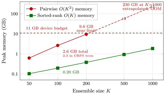
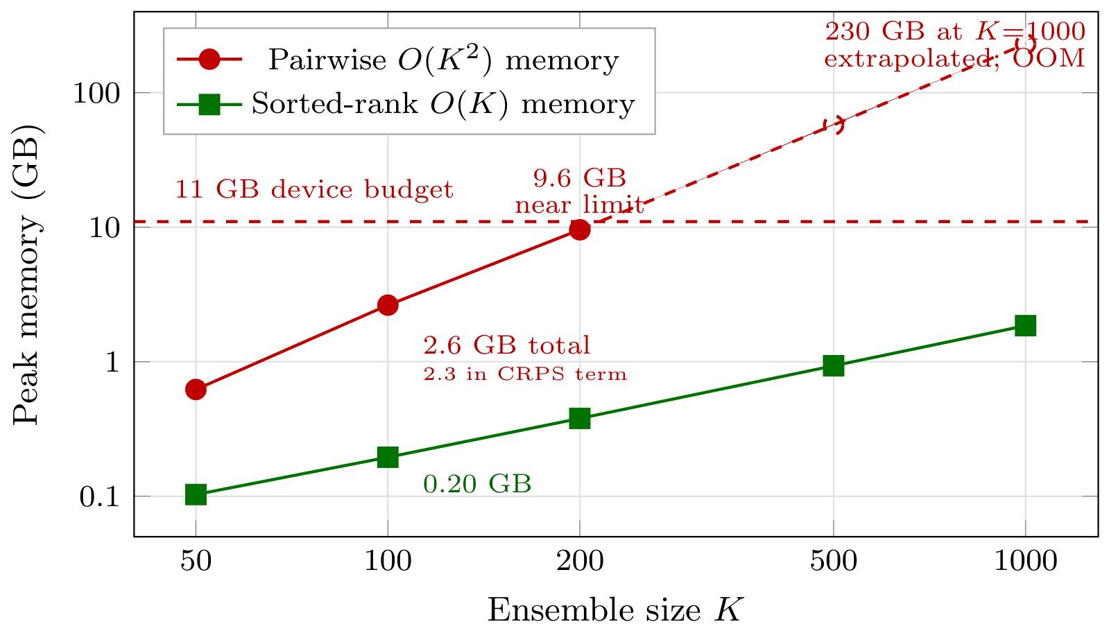
Figure 4 profiles the peak GPU memory of the objective as the ensemble grows from 50 to 1000 members. The sorted-rank form replaces the pairwise comparison tensor with the rank-weighted sum, dropping the total to 0.20 GB at 100 members, so the model capacity sets the ensemble the student is calibrated against; the pairwise form saturates the device at about 200 members and is out of memory from 500 onwards, while the sorted form needs 1.85 GB at 1000.

Figure 4. Peak GPU memory of the two CRPS estimators as the ensemble size grows, for $N=400$ evaluation windows, $H=288$, half precision, on an 11 GB device. The pairwise form materialises an $(N,H,K,K)$ tensor and grows quadratically: at the $K=100$ operating point it needs 2.6 GB, of which 2.3 GB is the pairwise term alone. At $K=200$, it uses 9.6 GB, approaching the 11 GB device budget, and it is out of memory from $K=500$ onwards, with 230 GB extrapolated at $K=1000$. The sorted-rank form stores only $(N,H,K)$ plus a sort workspace, so it grows linearly and stays below 2 GB even at $K=1000$. Both axes are logarithmic.

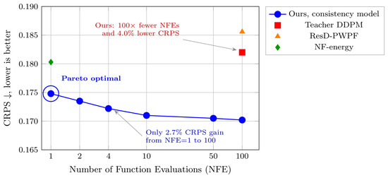
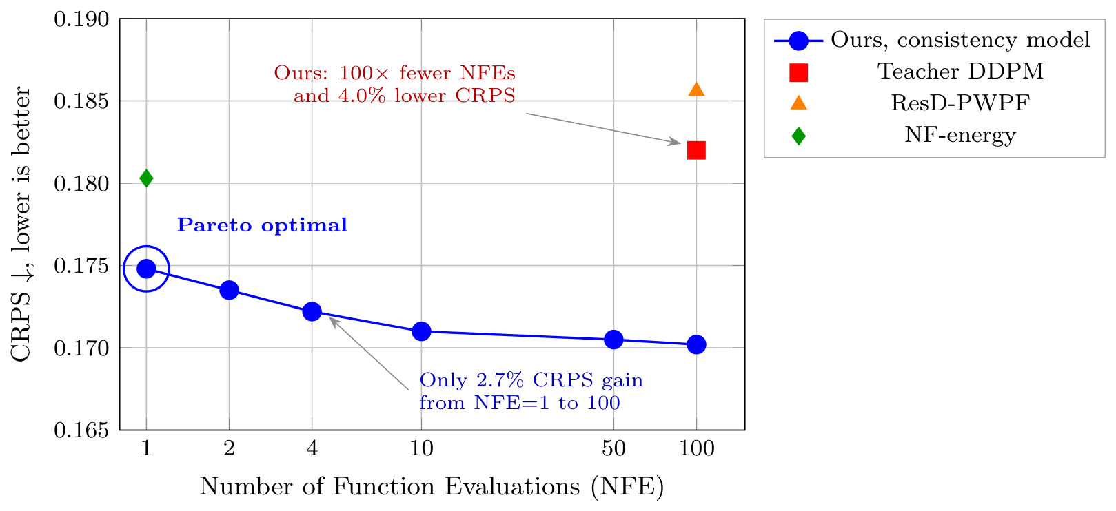
Figure 5 presents the accuracy-efficiency frontier in terms of the number of function evaluations. Increasing the number of evaluations from 1 to 100 improves CRPS from 0.1748 to 0.1702, a marginal 2.7% gain that costs 100× more computation. At a single evaluation, Consist-Wind dominates all baselines in this trade-off space. It uses the same single evaluation as the best normalizing flow, NF-energy with CRPS 0.1803, and is 3.1% more accurate. It is also 4.0% more accurate than the teacher DDPM, which needs 100 evaluations for CRPS 0.1820, and 65.6× faster. For operational forecasting with strict latency requirements, a single evaluation is the clear choice. The diminishing returns beyond it validate the consistency distillation strategy.

Figure 5. NFE–accuracy trade-off on GEFCom2014-W, pooled over 10 zones, under the same settings as Table 6. The blue curve shows Consist-Wind with varying NFE $\in \{1,2,4,10,50,100\}$: CRPS improves from 0.1748 at NFE = 1 to 0.1702 at NFE = 100, a marginal 2.7% gain. Red square: teacher DDPM at NFE = 100, CRPS 0.1820. Orange triangle: ResD-PWPF baseline, NFE = 100, CRPS 0.1856. Green diamond: NF-energy normalizing flow, NFE = 1, CRPS 0.1803. Pareto optimality. Consist-Wind at NFE = 1, circled, dominates all other methods in the accuracy-efficiency trade-off space, achieving competitive CRPS with 100× fewer evaluations than diffusion baselines. Increasing NFE beyond one yields diminishing returns: the full 100-fold increase from NFE = 1 to NFE = 100 lowers CRPS by only 2.7%. Under a ten-minute rolling update cycle, NFE = 1 is therefore the operating point of choice.

5.4. Calibration Quality

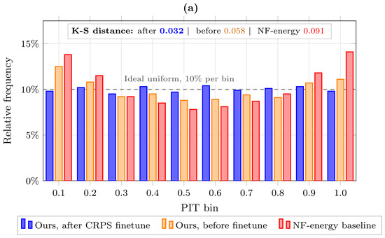
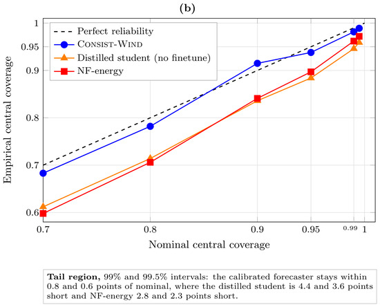
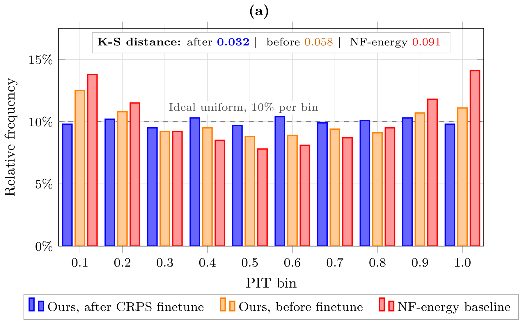
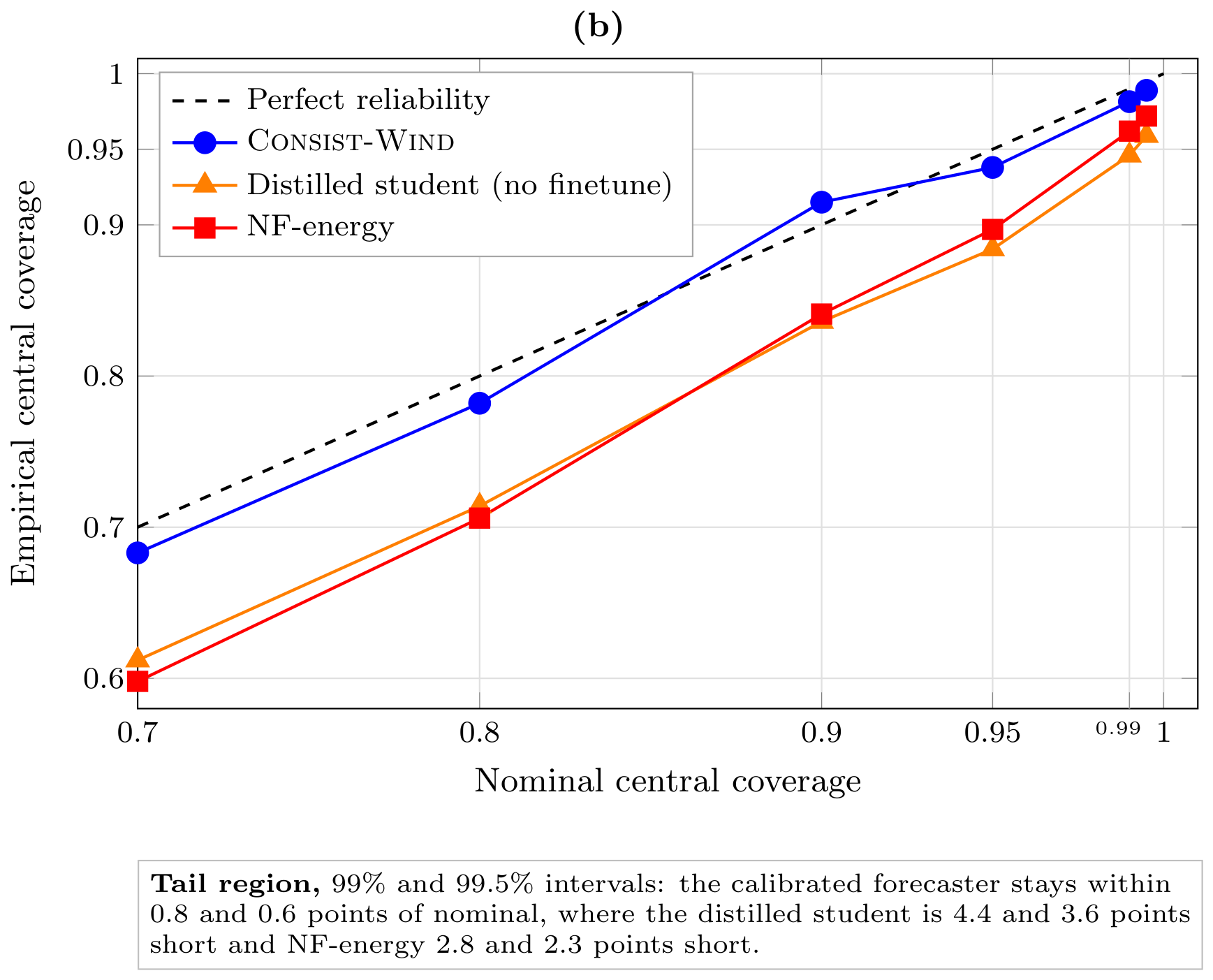
Figure 6 shows the Probability Integral Transform (PIT) histograms on the GEFCom2014-W test set, and Table 8 reports the calibration metrics. After CRPS fine-tuning, Consist-Wind is well calibrated: the mean absolute coverage deviation is 1.8% for the 80% interval and 1.5% for the 90% interval, the PIT histogram is close to uniform with a Kolmogorov–Smirnov distance of 0.032, and reliability is on par with the multi-step teacher. In contrast, the distilled student before fine-tuning shows a U-shaped PIT with K–S distance 0.058, and the NF-energy baseline shows a K–S distance of 0.091. The tails are calibrated as well: the 95%, 99%, and 99.5% intervals attain empirical coverages of 0.938, 0.982, and 0.989 (Table 8), and the reliability diagram of Figure 6b tracks the diagonal across the extreme quantiles, where the operational risk concentrates and the reproduced baselines depart.

Figure 6. Probability Integral Transform (PIT) histogram and reliability diagram on the GEFCom2014-W test set, pooled over 10 zones. (a) The PIT value for each observation is its empirical CDF rank within the forecast ensemble: $\mathrm{PIT}\left(y\right)={\displaystyle \frac{1}{K}}{\sum }_{k=1}^K\mathbb{I}[s_k\le y]$. A well-calibrated probabilistic forecast yields a near-uniform PIT distribution, 10% per bin, shown as the gray dashed line. Ours, after CRPS fine-tuning, blue: near-uniform distribution with Kolmogorov–Smirnov (K–S) distance 0.032, indicating close agreement with the nominal coverage. Ours, before fine-tuning, orange: slight U-shape with K–S 0.058 shows overconfidence in tails after consistency distillation; the extreme quantiles 0.1 and 0.9 are overrepresented. NF-energy baseline, red: pronounced U-shape with K–S 0.091 reveals systematic miscalibration. Phase 4 CRPS fine-tuning successfully recovers calibration, reducing the K–S distance by 45% relative to the post-distillation model. This validates the necessity of the sorted-rank CRPS objective for maintaining distributional reliability in one-step sampling. (b) Empirical against nominal central coverage from the 70% to the 99.5% interval: the calibrated forecaster stays within one point of the diagonal across the range, including the 95%, 99%, and 99.5% intervals, while the distilled student before fine-tuning and the reproduced NF-energy baseline depart from it in the tail.

Table 8. Calibration results on the GEFCom2014-W test set with 10 zones.

Interval	Nominal	Empirical	$\left|\mathsf{\Delta }\right|$
80%	0.800	0.782	1.8%
90%	0.900	0.915	1.5%
95%	0.950	0.938	1.2%
99%	0.990	0.982	0.8%
99.5%	0.995	0.989	0.6%

5.5. Efficiency and Scaling

All efficiency experiments in this section follow one experiment setting: half precision, a single batched forward pass for the whole member set, and means over repeated batches after warm-up; the ensemble-size sweeps span the deployment point $K=100$, its doubling, and the next order of magnitude up to $K=1000$.

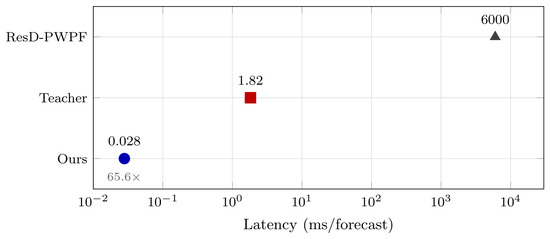
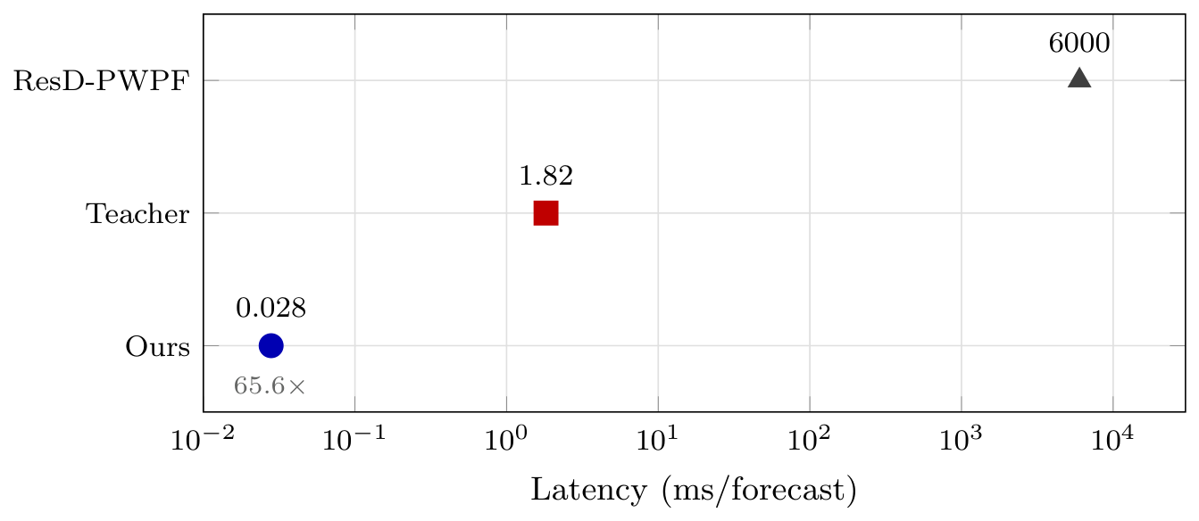
Wall-clock speedup. The efficiency measurements of this section run under query-chunked attention (QCA), which keeps every kernel launch within the device limit (chunks of at most 512 rows, Table 9); the attention peak memory then follows Equation (11) and grows with the chunk width, and all SDWPF and $H=288$ runs complete in this configuration. Figure 7 compares the per-forecast latency. Consist-Wind needs 0.028 ms per forecast for the $K=100$ ensemble at $H=48$, against 1.82 ms for the teacher at $T=100$, a measured 65.6× speedup. Each per-forecast time divides the wall-clock time of a batch of $B=64$ forecasts by the batch size, measured in FP16 on an RTX 2080 Ti (11 GB); the timings cover the forward pass only and exclude preprocessing and postprocessing. The ResD-PWPF value is a contextual reference quoted from its original setting (about 6 s per 24-h forecast on a MacBook Pro [9]); hardware and batching differ, so it is not a like-for-like speedup. Under the same settings, a $K=100$ ensemble is issued in 0.054 ms on an NVIDIA T4 and 0.21 ms on a GTX 1660, with the peak footprint below 5 GB, so the pipeline also runs on a 6 GB consumer card. The per-forecast time stays orders of magnitude inside the dispatch cycle on every device, so the limited-compute claims hold across three hardware generations, including a card without tensor cores.

Table 9. Horizon extension for query-chunked attention on GEFCom2014-W with all other settings fixed (ten zones, 400 pooled evaluation windows, patch window 8 with stride 4, chunks of at most 512 rows, low-rank context 16, FP16). The lookback extends with the horizon as $L=H+120$; “Attention rows” is the patched query batch $NP$; the standard peak is the fully materialized attention map of the unchunked form and “Saving” its ratio to the chunked workspace. Every configuration runs on the 11 GB device.

H	Attention Rows	Chunks	QCA Peak	Standard Peak	Saving
48	16,400	33	17.3 MB	538 MB	31×
96	21,200	42	22.4 MB	899 MB	40×
192	30,800	61	32.5 MB	1.90 GB	58×
288	40,400	79	42.7 MB	3.26 GB	76×
384	50,000	98	52.8 MB	5.00 GB	95×
480	59,600	117	62.9 MB	7.10 GB	113×

Figure 7. Per-forecast wall-clock latency on a logarithmic ordinate, measured on a single consumer GPU with 11 GB of memory with the $K=100$ ensemble, the $H=48$ horizon, and batch size $B=64$, as the mean over 100 forecasts after warm-up. Consist-Wind achieves a 65.6× speedup over the teacher DDPM. The ResD-PWPF bar is a contextual value quoted from its original setting, about 6 s per 24-h probabilistic forecast for one wind farm on a MacBook Pro (Apple M3 Max) [9]; hardware and batching differ, so it is not a like-for-like speed comparison. Error bars are omitted; the run-to-run standard deviation is below 1% of the mean over three repetitions.

Memory of the objective. Table 10 reports the peak memory of the calibration objective across ensemble sizes, complementing the breakdown of Figure 4 with the per-size values.

Table 10. Peak GPU memory in GB of the CRPS objective as the ensemble size K grows, with $N=400$, $H=288$, FP16, on an 11 GB device. The objective tensor is rebuilt at every update of the calibration phase.

Estimator	$\mathit{K}=50$	$\mathit{K}=100$	$\mathit{K}=200$	$\mathit{K}=500$	$\mathit{K}=1000$
Pairwise memory $O\left(K^2\right)$	0.62	2.6	9.6	OOM	OOM
Sorted-rank memory $O\left(K\right)$	0.10	0.20	0.38	0.93	1.85
Reduction	83%	93%	96%	—	—

Cost per evaluation of the objective. Table 11 reports the wall-clock cost and the numerical agreement of the two estimators. The sorted-rank form is 7.6× faster at 100 members and 9.1× at 200, since its $O\left(K\log K\right)$ cost grows slower than the quadratic pairwise form, which is out of memory at 500. It differs from the pairwise form only by floating-point round-off, a maximum absolute deviation of $3.2\times {10}^{-5}$ over 100 batches in half precision, consistent with Equation (5); the two forms therefore optimize the same loss.

Table 11. Wall-clock cost and numerical agreement of the two CRPS estimators with $N=400$, $H=288$, FP16, on an 11 GB device. Time is the mean per-call latency over 100 benchmark batches, with one scorer call per batch; deviation is measured against the pairwise reference over the same batches. Dashes mark configurations where the pairwise scorer exceeds the device budget.

Estimator	$\mathit{K}=50$	$\mathit{K}=100$	$\mathit{K}=200$	$\mathit{K}=500$	$\mathit{K}=1000$
Pairwise $O\left(K^2\right)$ (ms)	5.0	19.3	76.8	—	—
Sorted-rank $O\left(K\log K\right)$ (ms)	1.9	2.6	8.4	13.0	20.9
Speed-up	2.7×	7.6×	9.1×	—	—
Max deviation	$3.2\times {10}^{-5}$	$2.1\times {10}^{-5}$	$1.7\times {10}^{-5}$	—	—

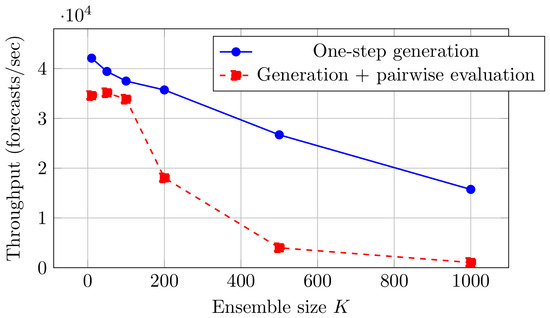
Throughput scaling. Figure 8 plots the throughput in forecasts per second against the ensemble size K. Consist-Wind generates 15,700 forecasts per second at $K=1000$, orders of magnitude above the needs of a 100-turbine farm on a 10-min cycle; the pairwise objective collapses the throughput beyond $K\approx 200$.

Figure 8. Throughput scaling with the ensemble size K, measured on a single consumer GPU (11 GB) with batch size $B=64$ and $H=48$. The blue curve is the one-step ensemble generation of Consist-Wind: throughput declines gradually from 42,100 forecasts per second at $K=10$ to 15,700 at $K=1000$, enough for real-time operation of a 100-turbine farm on a 10-min update cycle. The red dashed curve adds the pairwise objective evaluation, whose quadratic $O\left(K^2\right)$ penalty term dominates the batch cost beyond $K\approx 200$ and leaves 1050 forecasts per second at $K=1000$.

The advantage of query-chunked attention grows with the horizon: on GEFCom2014-W with all other settings fixed, its workspace saving over the materialized attention map rises from 31× at $H=48$ to 113× at $H=480$ (Table 9), because the chunked workspace grows linearly while the materialised map grows quadratically, and every launch stays bounded at 512 rows.

5.6. Comparison with Prior Fast Sampling Methods

Table 12 compares Consist-Wind with fast-sampling baselines reimplemented under our GEFCom2014-W setup. In this experiment, progressive distillation [29] reaches four evaluations with a CRPS of 0.1685, 1.8% above the teacher, and DDIM [30] reaches 10 evaluations with a CRPS of 0.1708, 3.2% above the teacher. Both methods use the teacher’s objective. Consistency distillation combined with CRPS fine-tuning reaches a single evaluation and improves on the teacher by 4.0% in the same setup, since phase 4 optimizes the scoring rule itself.

Table 12. Results from our fast-sampling implementations on GEFCom2014-W zone 1. The reproduced teacher DDPM at $T=100$ has CRPS 0.1655.

Method	NFE	CRPS	Rel. Change
Teacher DDPM	100	0.1655	–
Progressive distill [29]	4	0.1685	+1.8%
DDIM [30]	10	0.1708	+3.2%
Consist-Wind, consistency	1	0.1589	−4.0%

Consistency distillation provides a principled one-step objective: the self-consistency property learns the fixed point of the probability flow ODE [11], and the bounded-power warp keeps that fixed point inside the physical range $[0,1]$. In our reproduction, the one-step student improves on the teacher by 4.0% at a single evaluation, whereas progressive distillation still pays 1.8% at four evaluations and DDIM 3.2% at ten.

5.7. Parameter Sensitivity

Table 13 and Table 14 sweep the key parameters at the pilot and full scale, respectively. The defaults are kept: $\tau =1.0$, flat across $\tau \in [1.0,1.5]$ (the best tested $\tau =1.2$ within one standard deviation) but degrading by 3.4% at $\tau =0.8$ and 10.9% at $\tau =0.6$; 4000 distillation steps, monotone and saturating (under 1% gained to 8000 steps, 2.8% lost at 1000); and 400 fine-tuning steps, within 0.6% of the best tested configuration, with longer budgets degrading the score. The temperature also sets the ensemble width: the mean 95% interval widens from 0.62 to 0.98, and the $q=0.95$ pinball loss improves from 0.086 at $\tau =0.6$ to 0.075 at $\tau =1.0$. The shifted-logit warp is kept for its finite boundary mass (Section 3.3): arctanh and probit diverge at the boundaries, and the beta-warp adds shape parameters without a gain; removing the warp costs 2.7% CRPS and the physical bound (Table 5).

Table 13. Parameter sensitivity at the pilot scale (zone 1 of GEFCom2014-W, validation split, $L=168$, $H=48$, $K=100$, 400 evaluation windows, mean ± standard deviation over three seeds). Top block: warp temperature $\tau$. Bottom block: consistency-distillation budget. Default values are marked with an asterisk.

Setting	CRPS ↓
Warp temperature τ
0.6	0.1663 ± 0.0008
0.8	0.1551 ± 0.0009
1.0 *	0.1500 ± 0.0014
1.2	0.1485 ± 0.0017
1.5	0.1499 ± 0.0020
Distillation steps
1000	0.1542 ± 0.0024
2000	0.1511 ± 0.0014
4000 *	0.1500 ± 0.0014
8000	0.1484 ± 0.0001

Table 14. CRPS-fine-tuning budget and learning rate at the full-scale setting (GEFCom2014-W, ten zones, $L=168$, $H=48$, $K=100$, mean ± standard deviation over three seeds); the reported full-scale score is 0.1748. Default values are marked with an asterisk.

Steps	Learning Rate	CRPS ↓
400 *	$1\times {10}^{-4}$ *	0.1748 ± 0.0020
1600	$1\times {10}^{-4}$	0.1747 ± 0.0021
3200	$1\times {10}^{-4}$	0.1765 ± 0.0024
400	$5\times {10}^{-4}$	0.1738 ± 0.0019
1600	$5\times {10}^{-5}$	0.1746 ± 0.0020

6. Discussion

6.1. Interpretation of the Results

The calibrated one-step student surpasses the diffusion teacher it distills from (0.1589 against 0.1655) at one hundredth of the evaluations per member, and the ablation attributes this outcome to the calibration phase. The mechanism is metric alignment: pointwise distillation leaves the distribution over the noise input free, so the distilled ensemble is under-dispersed (coverage error 4.2% against 1.8% after calibration), and the calibration phase optimizes the proper scoring rule used for evaluation on the student’s own ensemble [15,31]. Because that rule is minimized only by the true predictive distribution, training on it restores the spread lost in distillation [13,14], which is why a student optimized on the metric itself exceeds its teacher. A less anticipated pattern runs through the ablations: the scores are insensitive to the settings around the operating point—the estimator swap and the attention restructure leave CRPS and coverage unchanged, and the parameter sweeps are flat—so the efficiency comes at no measured accuracy cost.

6.2. Practical Implications of the Efficiency Gains

Faster inference and smaller memory widen the range where the forecaster can be deployed. A $K=100$ ensemble is issued in 0.028 ms, so the full forecast fits easily inside the 10-min dispatch cycle, and the model can run at the point of use—an edge controller or a substation server—and be refreshed far more often, keeping the short-horizon forecast current. On the training side, 1.85 GB suffices for a $K=1000$ calibration, so one consumer GPU covers ensemble sizes the pairwise objective would put beyond hundreds of gigabytes. Both savings lower the hardware and energy cost of deployment and allow larger, more accurate ensembles.

6.3. Limitations and Outlook

Where the framework is applied beyond the benchmark settings studied here, several limitations should be anticipated. A new wind farm may differ in terrain and turbine characteristics, so accuracy can drop without local adaptation; horizons longer than those studied fall outside the scales of the patch structure and the warp window; rare weather regimes are under-represented in training, so intervals can be too narrow exactly in extreme events; deployment depends on the availability and latency of weather inputs, while the model ages as the farm changes. These limitations are the natural targets of further work—on-site calibration or transfer for new farms, horizon-conditioned temporal scales, regime-aware calibration and conservative spread under distribution shift, and online drift detection in operation. We leave these extensions to future work.

7. Conclusions

Probabilistic wind power forecasting benefits from low-latency sampling and memory-efficient ensemble calibration under limited computing resources. The Consist-Wind forecaster combines these properties in one pipeline. A frozen point backbone supplies the point forecast and the conditioning context; a residual diffusion teacher is distilled into a one-step consistency student, so each ensemble member is drawn in one forward pass; a stabilized shifted-logit warp maps the residual coordinate to a numerically controlled representation and returns generated members to the physical power range; and a final phase calibrates the student with a sorted-rank CRPS objective whose memory grows linearly with the ensemble size, while query-chunked attention and half-precision training keep the whole pipeline within a limited compute budget. In our experiments on GEFCom2014-W, SDWPF, and GEFCom2012-W, Consist-Wind attains the lowest CRPS on all three datasets, improves on the strongest reproduced baseline by 3.1%, reduces the calibration error of the distilled student by 45%, issues a forecast in 0.03 ms, and reduces the memory required to evaluate the pairwise penalty term by 98%, enabling 500-member calibration ensembles on the evaluation device. The same design carries over to other bounded power and load forecasting settings that need accurate distributions at low inference cost, and the linear-memory calibration objective transfers to any forecaster trained with a proper scoring rule on a resource-constrained device.

References

- Sánchez, I. Short-term prediction of wind energy production. Int. J. Forecast. 2006, 22, 43–56. [Google Scholar] [CrossRef] [Scilit]
- Hong, T.; Pinson, P.; Fan, S.; Zareipour, H.; Troccoli, A.; Hyndman, R.J. Probabilistic energy forecasting: Global Energy Forecasting Competition 2014 and beyond. Int. J. Forecast. 2016, 32, 896–913. [Google Scholar] [CrossRef] [Scilit]
- Hong, T.; Pinson, P.; Fan, S. Global Energy Forecasting Competition 2012. Int. J. Forecast. 2014, 30, 357–363. [Google Scholar] [CrossRef] [Scilit]
- Maciejowska, K.; Nowotarski, J.; Weron, R. Probabilistic forecasting of electricity spot prices using factor quantile regression averaging. Int. J. Forecast. 2016, 32, 957–965. [Google Scholar] [CrossRef] [Scilit]
- Salinas, D.; Flunkert, V.; Gasthaus, J.; Januschowski, T. DeepAR: Probabilistic forecasting with autoregressive recurrent networks. Int. J. Forecast. 2020, 36, 1181–1191, Erratum in Int. J. Forecast. 2021, 37, 1302–1303. https://doi.org/10.1016/j.ijforecast.2021.01.010. [Google Scholar] [CrossRef] [Scilit]
- Lim, B.; Arık, S.Ö.; Loeff, N.; Pfister, T. Temporal fusion transformers for interpretable multi-horizon time series forecasting. Int. J. Forecast. 2021, 37, 1748–1764. [Google Scholar] [CrossRef] [Scilit]
- Dumas, J.; Wehenkel, A.; Lanaspeze, D.; Cornélusse, B.; Sutera, A. A deep generative model for probabilistic energy forecasting in power systems: Normalizing flows. Appl. Energy 2022, 305, 117871. [Google Scholar] [CrossRef] [Scilit]
- Hernandez Capel, E.; Dumas, J. Denoising diffusion probabilistic models for probabilistic energy forecasting. In Proceedings of the 2023 IEEE Belgrade PowerTech, Belgrade, Serbia, 25–29 June 2023; IEEE: New York, NY, USA, 2023; pp. 1–6. [Google Scholar] [CrossRef] [Scilit]
- Chen, F.; Gao, L. Learning residual distributions with diffusion models for probabilistic wind power forecasting. Energies 2025, 18, 4226. [Google Scholar] [CrossRef] [Scilit]
- Gong, M.; Tian, Y.; Zhang, F.; Yin, S.; Sun, M.; Wang, Y.; Zhu, L.; Zhang, Y.; Xu, W. DiffWPF: A diffusion-based model for multi-step probabilistic wind power forecasting. Electr. Power Syst. Res. 2026, 260, 113347. [Google Scholar] [CrossRef] [Scilit]
- Song, Y.; Dhariwal, P.; Chen, M.; Sutskever, I. Consistency Models. In Proceedings of the 40th International Conference on Machine Learning, Honolulu, HI, USA, 23–29 July 2023; PMLR: New York, NY, USA, 2023; Proceedings of Machine Learning Research; Volume 202, pp. 32211–32252. Available online: https://proceedings.mlr.press/v202/song23a.html (accessed on 10 February 2026).
- Luo, S.; Tan, Y.; Huang, L.; Li, J.; Zhao, H. Latent consistency models: Synthesizing high-resolution images with few-step inference. arXiv 2023, arXiv:2310.04378. [Google Scholar]
- Stock, J.; Arcomano, T.; Kotamarthi, R. Swift: An autoregressive consistency model for efficient weather forecasting. Mach. Learn. Earth 2026, 2, 025004. [Google Scholar] [CrossRef] [Scilit]
- Garrepalli, R.; Mahajan, S.; Hayat, M.; Porikli, F. DDIL: Diversity Enhancing Diffusion Distillation with Imitation Learning. arXiv 2025, arXiv:2410.11971. [Google Scholar]
- Gneiting, T.; Raftery, A.E. Strictly proper scoring rules, prediction, and estimation. J. Am. Stat. Assoc. 2007, 102, 359–378. [Google Scholar] [CrossRef] [Scilit]
- Lang, S.; Leutbecher, M.; Maciel, P. A multi-scale loss formulation for learning a probabilistic model with proper score optimisation. Q. J. R. Meteorol. Soc. 2026; in press. [CrossRef] [Scilit]
- He, J.; Hu, Z. Probabilistic forecasting method for offshore wind farm cluster under typhoon conditions: A score-based conditional diffusion model. arXiv 2025, arXiv:2508.10705. [Google Scholar]
- Jonas, S.; Winter, K.; Brodbeck, B.; Meyer, A. Bias correction of wind power forecasts with SCADA data and continuous learning. J. Phys. Conf. Ser. 2024, 2767, 092061. [Google Scholar] [CrossRef] [Scilit]
- Zhang, Y.; Jiang, J.; Yan, Y.; Yang, L.; Zhang, P. 2DXformer: Dual transformers for wind power forecasting with dual exogenous variables. arXiv 2025, arXiv:2505.01286. [Google Scholar]
- Tan, L.; Yue, H. Application of BERT in wind power forecasting–Teletraan’s solution in Baidu KDD Cup 2022. arXiv 2023, arXiv:2307.09248. [Google Scholar]
- Jiang, J.; Han, C.; Wang, J. BUAA_BIGSCity: Spatial-temporal graph neural network for wind power forecasting in Baidu KDD Cup 2022. arXiv 2023, arXiv:2302.11159. [Google Scholar]
- Bahi, A.; Ourici, A.; Gasmi, I.; Derrablia, A.; Deghmane, W.; Ferrag, M.A. FreeGNN: Continual source-free graph neural network adaptation for renewable energy forecasting. Expert Syst. Appl. 2026, 332, 133456. [Google Scholar] [CrossRef] [Scilit]
- Bentsen, L.Ø.; Warakagoda, N.D.; Stenbro, R.; Engelstad, P. Spatio-temporal wind speed forecasting using graph networks and novel transformer architectures. Appl. Energy 2023, 333, 120565. [Google Scholar] [CrossRef] [Scilit]
- Wan, C.; Lei, S.; Luo, Y. Hiformer: Hybrid frequency feature enhancement inverted transformer for long-term wind power prediction. arXiv 2024, arXiv:2410.13303. [Google Scholar]
- Zim, A.H.; Iqbal, A.; Malik, A.; Dong, Z.; Wu, H. TCNFormer: Temporal convolutional network former for short-term wind speed forecasting. arXiv 2024, arXiv:2408.15737. [Google Scholar]
- Yuan, S.; Mao, Y.; Tian, C.; Yu, F.; Guo, T.; Xia, M. GSTAformer: Graph-guided spatio-temporal Autoformer for mid-term wind power forecasting. Energies 2026, 19, 254. [Google Scholar] [CrossRef] [Scilit]
- Wu, Z.; Shi, Y.; Guo, T.; Xia, M. VSTCformer for wind power interval forecasting via adaptive variational mode decomposition and spatio-temporal cross-attention. Appl. Sci. 2026, 16, 7470. [Google Scholar] [CrossRef] [Scilit]
- Zhang, Y.; Zhang, Z.; Hu, Y.; Wan, Y. GMD-Linear: Integrating graph neural networks and WaveNet for enhanced wind power forecasting. In Proceedings of the 2024 12th International Conference on Information Systems and Computing Technology (ISCTech), Xi’an, China, 8–11 November 2024; pp. 1–5. [Google Scholar] [CrossRef] [Scilit]
- Salimans, T.; Ho, J. Progressive Distillation for Fast Sampling of Diffusion Models. In Proceedings of the 10th International Conference on Learning Representations, Online, 25–29 April 2022; Available online: https://openreview.net/forum?id=TIdIXIpzhoI (accessed on 10 February 2026).
- Song, J.; Meng, C.; Ermon, S. Denoising Diffusion Implicit Models. In Proceedings of the 9th International Conference on Learning Representations, Online, 3–7 May 2021; Available online: https://openreview.net/forum?id=St1giarCHLP (accessed on 10 February 2026).
- Ferro, C.A.T. Fair scores for ensemble forecasts. Q. J. R. Meteorol. Soc. 2014, 140, 1917–1923. [Google Scholar] [CrossRef] [Scilit]
- Gneiting, T.; Ranjan, R. Comparing density forecasts using threshold- and quantile-weighted scoring rules. J. Bus. Econ. Stat. 2011, 29, 411–422. [Google Scholar] [CrossRef] [Scilit]
- Allen, S.; Bhend, J.; Martius, O.; Ziegel, J. Weighted verification tools to evaluate univariate and multivariate probabilistic forecasts for high-impact weather events. Weather Forecast. 2023, 38, 499–516. [Google Scholar] [CrossRef] [Scilit]
- Zamo, M.; Naveau, P. Estimation of the continuous ranked probability score with limited information and applications to ensemble weather forecasts. Math. Geosci. 2018, 50, 209–234. [Google Scholar] [CrossRef] [Scilit]
- Lerch, S.; Thorarinsdottir, T.L.; Ravazzolo, F.; Gneiting, T. Forecaster’s dilemma: Extreme events and forecast evaluation. Stat. Sci. 2017, 32, 106–127. [Google Scholar] [CrossRef] [Scilit]
- Pinson, P.; Tastu, J. Discrimination Ability of the Energy Score; Technical Report 15; Technical University of Denmark: Kongens Lyngby, Denmark, 2013; Available online: https://orbit.dtu.dk/en/publications/discrimination-ability-of-the-energy-score/ (accessed on 10 February 2026).
- Taillardat, M.; Mestre, O.; Zamo, M.; Naveau, P. Calibrated ensemble forecasts using quantile regression forests and ensemble model output statistics. Mon. Weather Rev. 2016, 144, 2375–2393. [Google Scholar] [CrossRef] [Scilit]
- Jordan, A. Facets of Forecast Evaluation. Ph.D. Thesis, Karlsruhe Institute of Technology, Karlsruhe, Germany, 2016. [Google Scholar] [CrossRef]
- Hersbach, H. Decomposition of the continuous ranked probability score for ensemble prediction systems. Weather Forecast. 2000, 15, 559–570. [Google Scholar] [CrossRef] [Scilit]
- Chen, T.; Xu, B.; Zhang, C.; Guestrin, C. Training deep nets with sublinear memory cost. arXiv 2016, arXiv:1604.06174. [Google Scholar]
- Han, S.; Mao, H.; Dally, W.J. Deep Compression: Compressing Deep Neural Networks with Pruning, Trained Quantization and Huffman Coding. In Proceedings of the 4th International Conference on Learning Representations, San Juan, Puerto Rico, 2–4 May 2016. [Google Scholar] [CrossRef] [Scilit]
- Sheng, L.; Fu, N.; Mou, J.; Zhu, L.; Zhou, J. Data-driven probabilistic wind power forecasting and dispatch with alternating direction method of multipliers over complex networks. Mathematics 2026, 14, 112. [Google Scholar] [CrossRef] [Scilit]
- Liu, Y.; Hu, T.; Zhang, H.; Wu, H.; Wang, S.; Ma, L.; Long, M. iTransformer: Inverted Transformers Are Effective for Time Series Forecasting. In Proceedings of the 12th International Conference on Learning Representations, Vienna, Austria, 7–11 May 2024; Volume 2024, pp. 11116–11140. Available online: https://proceedings.iclr.cc/paper_files/paper/2024/hash/2ea18fdc667e0ef2ad82b2b4d65147ad-Abstract-Conference.html (accessed on 10 February 2026).
- Perez, E.; Strub, F.; de Vries, H.; Dumoulin, V.; Courville, A. FiLM: Visual reasoning with a general conditioning layer. In Proceedings of the 32nd AAAI Conference on Artificial Intelligence, New Orleans, LA, USA, 2–7 February 2018; Volume 32, pp. 3942–3951. [Google Scholar] [CrossRef] [Scilit]
- Ho, J.; Jain, A.N.; Abbeel, P. Denoising Diffusion Probabilistic Models. In Proceedings of the Advances in Neural Information Processing Systems; Curran Associates, Inc.: Red Hook, NY, USA, 2020; Volume 33, pp. 6840–6851. Available online: https://papers.nips.cc/paper/2020/hash/4c5bcfec8584af0d967f1ab10179ca4b-Abstract.html (accessed on 10 February 2026).
- Grover, A.; Wang, E.J.; Zweig, A.; Ermon, S. Stochastic Optimization of Sorting Networks via Continuous Relaxations. In Proceedings of the 7th International Conference on Learning Representations, New Orleans, LA, USA, 6–9 May 2019; Available online: https://openreview.net/forum?id=H1eSS3CcKX (accessed on 10 February 2026).
- Zadrozny, B.; Elkan, C. Transforming classifier scores into accurate multiclass probability estimates. In Proceedings of the 8th ACM SIGKDD International Conference on Knowledge Discovery and Data Mining, Edmonton, AB, Canada, 23–26 July 2002; pp. 694–699. [Google Scholar] [CrossRef] [Scilit]
- Zhou, J.; Lu, X.; Xiao, Y.; Tang, J.; Su, J.; Li, Y.; Liu, J.; Lyu, J.; Ma, Y.; Dou, D. SDWPF: A dataset for spatial dynamic wind power forecasting over a large turbine array. Sci. Data 2024, 11, 649. [Google Scholar] [CrossRef] [Scilit] [PubMed]
Disclaimer/Publisher’s Note: The statements, opinions and data contained in all publications are solely those of the individual author(s) and contributor(s) and not of MDPI and/or the editor(s). MDPI and/or the editor(s) disclaim responsibility for any injury to people or property resulting from any ideas, methods, instructions or products referred to in the content. |
© 2026 by the authors. Licensee MDPI, Basel, Switzerland. This article is an open access article distributed under the terms and conditions of the Creative Commons Attribution (CC BY) license.