Synchronization in Probability of Reaction–Diffusion Neural Networks Under Stochastic Sampling Governed by Infinite Discrete Distributions

Abstract

This paper generalizes stochastic sampled-data synchronization of reaction–diffusion neural networks (RDNNs) from sampling distributions with finite support to infinite discrete distributions, whose sampling intervals are drawn from a countably infinite set ${\left\{q_i\right\}}_{i=1}^{\infty }$ with probabilities ${\left\{{\alpha }_i\right\}}_{i=1}^{\infty }$. Four regularity conditions are identified—finite interval mean, summability of the weighted absolute decay parameters, strict positivity of the probability-averaged decay rate, and boundedness above of the decay parameters, which makes the Lyapunov–Krasovskii functional (LKF) mode-independent in its delay weight and hence continuous across sampling instants. A mode-dependent LKF is constructed, the weak-law step is replaced by the strong law of large numbers combined with a Cesàro-type argument, and the infinite family of design linear matrix inequalities (LMIs) is handled by a truncation-with-tail-verification procedure, for which a rigorous certificate is given: when the tail decay parameters are non-positive, the tail conditions are affine and are certified by corner-point feasibility checks with shared variables; otherwise, a convergent-tail argument applies. Almost-sure exponential synchronization with an explicit rate is established, which implies synchronization in probability, and controller design conditions are derived in terms of LMIs; three examples (two neural networks and one reaction–diffusion neural network) corroborate the design through computed gains, verified tail conditions, stochastic closed-loop simulations, an N-sensitivity analysis, and a comparison with a fixed-period controller. The proposed framework removes the finite-support restriction on the sampling distribution and yields an almost-sure, rate-explicit synchronization guarantee with a numerically verifiable LMI design.

1. Introduction

Neural networks (NNs) have attracted sustained attention since Hopfield proposed the first collective computational model [1] and Chua and Yang introduced cellular NNs [2]. NNs offer large storage capacity, strong self-learning ability, associative memory, and powerful optimization capability, and they have been applied to model identification, pattern recognition, signal processing, and combinatorial optimization; recent representative studies include exponential synchronization with dynamic coding [3], dissipativity analysis of fractional-order memristive NNs [4], and disturbance-rejection stabilization of delayed memristive NNs [5]. Among the dynamical properties of coupled NNs, synchronization plays a distinguished role because it underpins secure communication, image processing, and the modeling of collective behavior in biological and engineered networks. In hardware and networked implementations, coupling is realized by digital controllers acting at discrete sampling instants, and the intervals between consecutive instants are frequently uncertain. A realistic description of this uncertainty is a stochastic sampling.

Reaction–diffusion NNs (RDNNs) extend NNs by incorporating the spatial diffusion of the neuron state. Turing’s seminal analysis [6] showed that reaction–diffusion mechanisms can destabilize otherwise uniform patterns, so the dynamical analysis of RDNNs is both challenging and practically relevant. A large body of results on RDNNs has appeared, covering impulsive synchronization with mixed delays and an image-encryption application [7], impulsive synchronization of stochastic RDNNs [8], quasi-synchronization under sampled-data control [9], adaptive event-triggered synchronization [10], fuzzy adaptive sampled-data stabilization [11], antisynchronization of multilayer RDNNs [12], global exponential synchronization of memristive RDNNs with multi-switching transmission [13], and synchronization criteria for switched delayed reaction–diffusion systems via impulsive control [14]. Because natural synchronization is difficult to achieve in the presence of diffusion and delay, control-based synchronization of RDNNs has become a central topic; representative sampled-data designs include finite-time synchronization with sampled-data communications [15], asynchronous sampled-data control for switched Markovian systems [16], improved fuzzy sampled-data stabilization [17], $H_{\infty }$ output synchronization [18], fuzzy sampled-data synchronization with additive delays [19], synchronization with spatial sampled-data [20], and quantized sampled-data designs under spatially point sampling [21].

Within the sampled-data literature, stochastic sampling has been studied for a wide range of problems. Gao et al. [22] established robust $H_{\infty }$ sampled-data control under stochastic sampling, Shen et al. [23] derived sampled-data synchronization criteria for dynamical networks with stochastically varying intervals, He et al. [24] treated leader-following consensus of nonlinear multi-agent systems, Du et al. [25] designed an observer-based consensus protocol, Su et al. [26] addressed time-varying formation control with communication delays, and Rakkiyappan et al. [27] analyzed synchronization of NNs with control packet loss and time-varying delay. In these works the random intervals are modeled either by continuous distributions or by discrete distributions with finite support. In particular, the recent switching-system protocol of Zeng et al. [28] established synchronization in probability for RDNNs under a finite discrete distribution $\mathbb{P}\{h_k=q_i\}={\alpha }_i$, $i=1,\dots ,N$, by attaching a switching parameter ${\rho }_{\sigma \left(t\right)}$ to the active subsystem, constructing a mode-dependent Lyapunov–Krasovskii functional (LKF), and invoking the weak law of large numbers.

Very recent developments continue to relax the assumptions on sampling and communication. Thomas et al. [29] analyzed exponential synchronization of nonlinear networked systems under asynchronous, aperiodic sampled-data coupling through a dissipativity-based input–output approach; Zhang et al. [30] proposed an accumulated-state-error-based event-triggered sampling scheme with a looped-functional analysis and co-designed the event-triggered controller for sampled-data systems; Chen et al. [31] studied exponential synchronization of RDNNs over directed networks via an asynchronous sampled-data event-triggered intermittent control scheme; Aili et al. [32] designed event-triggered controllers for synchronization of coupled NNs with reaction–diffusion terms; Zhang et al. [33] established exponential synchronization of coupled NNs with hybrid delays and stochastic distributed delayed impulses; and Liao et al. [34] addressed chaotic NN synchronization via sampled-data control under actuator saturation using a generalized looped functional. These works, however, model the sampling intervals as deterministic, bounded, or finite-support stochastic sequences, and their conclusions are formulated in the usual deterministic or mean-square senses. The present paper differs from all of them in two respects: the sampling intervals obey a countably infinite discrete distribution, and the synchronization conclusion is strengthened to almost-sure exponential decay with an explicit rate, obtained by replacing the weak-law step with the strong law of large numbers.

The finite-support assumption is convenient because the LKF conditions form a finite family of LMIs, but it excludes sampling models whose interval set is countably infinite—for example, geometric or Poisson-type interval laws arising from queues, retransmission counters, and long-tail communication links. In such models the support ${\left\{q_i\right\}}_{i=1}^{\infty }$ is infinite, the associated design conditions become an infinite family of LMIs, and the weak law of large numbers yields convergence in probability only (as $k\to \infty$). This paper removes the finite-support restriction. The main contributions are as follows.

• Infinite discrete sampling model with regularity conditions. We generalize the sampling model to a countably infinite set of intervals ${\left\{q_i\right\}}_{i=1}^{\infty }$ with probabilities ${\left\{{\alpha }_i\right\}}_{i=1}^{\infty }$, ${\sum }_{i=1}^{\infty }{\alpha }_i=1$, and identify four regularity conditions—finite interval mean (C1), summability of the weighted absolute decay parameters (C2), strict positivity of the probability-averaged decay rate (C3), and uniform boundedness of the LKF exponential weights (C4)—under which the synchronization analysis remains valid and is, moreover, strengthened.
• Almost-sure exponential synchronization with explicit rate. The main results (Theorems 1′–3′) show that the error system is exponentially synchronized in probability (as $t\to \infty$); by replacing the weak-law step of [28] with the strong law of large numbers combined with a Cesàro-type uniformity argument (Lemma 3), the conclusion is strengthened to almost-sure exponential decay of the LKF with the explicit rate $\varrho$ given by the probability-averaged switching parameter.
• Truncation with tail verification. Because the design conditions form an infinite family of LMIs, we propose a two-step numerical procedure: solve the LMIs for a truncated index set $\{1,\dots ,N\}$, then certify the remaining tail. When the tail decay parameters are non-positive, the tail conditions are affine in the tail parameters and are certified by corner-point feasibility checks with shared variables (Case A in Section 4.1); otherwise a convergent-tail argument applies (Case B). The procedure is demonstrated on two geometric laws with the closed-form tail masses $2^{-N}$ and ${(2/3)}^N$, and the convergence of the truncated design is examined by an N-sensitivity analysis and a comparison with a fixed-period controller.

Table 1 summarizes the differences between the finite-support framework of [28] and the present infinite-support framework; the numerical consequences are explored in Section 4.

Table 1. Comparison between the finite-support framework of [28] and the present infinite-support framework.

	[28]	This Paper
Sampling assumption	$\mathbb{P}\{h_k=q_i\}={\alpha }_i$, $i=1,\dots ,N$ (finite support)	$\mathbb{P}\{h_k=q_i\}={\alpha }_i$, $i=1,2,\dots$ (countably infinite support), (C1)–(C4)
Probabilistic conclusion	synchronization in probability (as $t\to \infty$), weak law	almost-sure exponential decay with explicit rate $\varrho$ (Definition 2), strong law + Cesàro argument
LKF structure	mode-dependent exponential weight in the delay term	mode-independent weight ${\rho }_0$ (C4); continuous across sampling instants
Design conditions	finite family of N LMIs	countably infinite family of LMIs
Numerical verification	N finite LMI constraints	truncation (S1) + tail certificate (S2), Case A (affine, corner-point checks with shared variables) or Case B (convergent tail)
Controller implementation	finite gains $K_1,\dots ,K_N$, one per sampled mode	gains $K_1,\dots ,K_N$ from (S1), shared tail gain $K_{\mathrm{tail}}=K_N$ for all modes $i>N$; implemented as $K_{{\sigma }_k}\vartheta (t_{k-1},x)$ on $[t_{k-1},t_k)$
Rate	not rate-explicit	$\varrho /2$ in the error estimate (26)

Notation. ${\mathbb{R}}^n$ denotes the n-dimensional Euclidean space; ${\lambda }_{min}(·)$ and ${\lambda }_{max}(·)$ denote the minimum and maximum eigenvalues of a symmetric matrix. For a matrix X, $X>0$ ($X\ge 0$) means X is symmetric positive-definite (semidefinite). $col\{v_1,\dots ,v_k\}$ stacks vectors, and $\parallel ·\parallel$ is the Euclidean norm of a vector or the induced norm of a matrix. For the RDNN case we write ${\parallel \vartheta (t,·)\parallel }_{L^2\left(\mathsf{\Omega }\right)}:={\left({\int }_{\mathsf{\Omega }}{\vartheta }^{\mathrm{T}}(t,x)\vartheta (t,x)dx\right)}^{1/2}$ for the spatial $L^2$ norm and ${\parallel \phi \parallel }_{★}^2:={sup}_{s\in [-\overline{d},0]}{\parallel \phi (s,·)\parallel }_{L^2\left(\mathsf{\Omega }\right)}^2+{\sum }_{l=1}^m{\parallel \partial \phi (0,·)/\partial x_l\parallel }_{L^2\left(\mathsf{\Omega }\right)}^2$ for the initial data $\phi (s,x)$, $s\in [-\overline{d},0]$; in the NN case (no spatial variable), ${\parallel \phi \parallel }_{★}^2:={sup}_{s\in [-\overline{d},0]}{\parallel \phi \left(s\right)\parallel }^2$.

Organization. Section 2 formulates the drive–response RDNNs, the infinite discrete sampling model, and the regularity conditions, and collects the auxiliary lemmas. Section 3 presents the synchronization and design criteria. Section 4 provides the numerical examples with the truncation and tail-verification procedure. Section 5 concludes the paper.

2. Problem Formulation and Preliminaries

2.1. Drive–Response RDNNs

Consider the drive system described by the reaction–diffusion neural network

$$\begin{array}{cc}\hfill {\displaystyle \frac{\partial y(t,x)}{\partial t}}& ={\displaystyle \sum _{l=1}^m}{A}_l{\displaystyle \frac{{\partial }^{2}y(t,x)}{\partial x_l^2}}-By(t,x)+C_{1}f\left(y(t,x)\right)\hfill \\ \hfill & +C_{2}f\left(y(t-d\left(t\right),x)\right)+J,\hfill \end{array}$$

(1)

where $x=col\{x_1,\dots ,x_m\}\in \mathsf{\Omega }$, $\mathsf{\Omega }$ is a bounded domain of ${\mathbb{R}}^m$ with smooth boundary $\partial \mathsf{\Omega }$, $y\in {\mathbb{R}}^n$ is the neuron state, $A_l=diag\{a_{l1},\dots ,a_{ln}\}\ge 0$ are the transmission diffusion coefficient matrices, $B=diag\{b_1,\dots ,b_n\}>0$, $C_1,C_2\in {\mathbb{R}}^{n\times n}$ are the connection weight matrices, $f(·)$ is the neuron activation function, $d\left(t\right)$ is a time-varying delay, and $J\in {\mathbb{R}}^n$ is a constant input. The drive system (1) evolves freely, and the sampled-data control input, defined below, is applied to the response system only. The boundary and initial conditions are

$$\begin{array}{c}y(t,x)=0,(t,x)\in [-\overline{d},\infty )\times \partial \mathsf{\Omega },\\ y(s,x)=\varphi (s,x),(s,x)\in [-\overline{d},0]\times \mathsf{\Omega }.\end{array}$$

(2)

The response system is

$$\begin{array}{cc}\hfill {\displaystyle \frac{\partial z(t,x)}{\partial t}}& ={\displaystyle \sum _{l=1}^m}{A}_l{\displaystyle \frac{{\partial }^{2}z(t,x)}{\partial x_l^2}}-Bz(t,x)+C_{1}f\left(z(t,x)\right)\hfill \\ \hfill & +C_{2}f\left(z(t-d\left(t\right),x)\right)+J+u(t,x),\hfill \end{array}$$

(3)

with the same diffusion, boundary, and initial conditions (with initial function $\psi$). The sampling instants are $t_0=0$ and $t_k={\sum }_{j=1}^k{h}_j$, $k\ge 1$, where $h_k:=t_k-t_{k-1}$ denotes the length of the k-th sampling interval $[t_{k-1},t_k)$; the random mechanism generating $\left\{h_k\right\}$ is specified in Assumption 3.

Assumption 1.

The activation function $f_i(·)$ satisfies $f_i\left(0\right)=0$ and, for all $s_1,s_2\in \mathbb{R}$, $s_1\ne s_2$,

$$0\le {\displaystyle \frac{f_i\left(s_1\right)-f_i\left(s_2\right)}{s_1-s_2}}\le l_i,i=1,\dots ,n,$$

for constants $l_i>0$. We set $L=diag\{l_1,\dots ,l_n\}$.

Assumption 2.

The delay $d\left(t\right)$ is continuously differentiable with $0\le d\left(t\right)\le \overline{d}$ and $\dot{d}\left(t\right)\le \mu <1$ for all $t\ge 0$.

Define the synchronization error $\vartheta (t,x)=z(t,x)-y(t,x)$. Subtracting (1) from (3) and using Assumption 1 with $g(·)=f(·)$ (the argument is standard; see, e.g., [28]), and noting that u acts on the response system only and therefore survives the subtraction, the error dynamics obey

$$\begin{array}{cc}\hfill {\displaystyle \frac{\partial \vartheta (t,x)}{\partial t}}& ={\displaystyle \sum _{l=1}^m}{A}_l{\displaystyle \frac{{\partial }^2\vartheta (t,x)}{\partial x_l^2}}-B\vartheta (t,x)+C_{1}g\left(\vartheta (t,x)\right)\hfill \\ \hfill & +C_{2}g\left(\vartheta (t-d\left(t\right),x)\right)+u(t,x),\hfill \end{array}$$

(4)

where $g\left(\vartheta \right)=f\left(z\right)-f\left(y\right)$ satisfies $g\left(0\right)=0$ and $0\le g_i\left(s\right)/s\le l_i$.

2.2. Stochastic Sampling with Infinite Discrete Distribution

The control input is a sampled-data controller of the switching form

$$u(t,x)=K_{{\sigma }_k}\vartheta (t_{k-1},x),t\in [t_{k-1},t_k),$$

(5)

where ${\sigma }_k\in \{1,2,\dots \}$ is the index of the subsystem active on $[t_{k-1},t_k)$ (defined in Assumption 3) and $K_i$ are the controller gain matrices to be designed.

Assumption 3.

At each sampling instant $t_{k-1}$ ($k\ge 1$), the length $h_k=t_k-t_{k-1}$ of the next sampling interval is drawn independently from the infinite

$$\mathbb{P}\{h_k=q_i\}={\alpha }_i,i=1,2,\dots ,{\alpha }_i>0,{\displaystyle \sum _{i=1}^{\infty }}{\alpha }_i=1,$$

(6)

with $0<q_i\le \overline{q}<\infty$ for all $i\ge 1$ and $q_i\to q_{\infty }:={lim}_{i\to \infty }{q}_i$. The mode index active on $[t_{k-1},t_k)$ is $\sigma \left(t\right)={\sigma }_k=i$ whenever $h_k=q_i$; since $h_k$ is drawn at $t_{k-1}$, the controller gain $K_{{\sigma }_k}$ is available on the whole interval $[t_{k-1},t_k)$.

Equation (6) is the infinite-support generalization of the finite model $\mathbb{P}\{h_k=q_i\}={\alpha }_i$, $i=1,\dots ,N$, of [28]; throughout the paper, a primed number denotes the infinite-distribution generalization of the homonymous equation in [28]. We impose the following regularity conditions.

Assumption 4.

The sequences $\left\{q_i\right\}$ and $\left\{{\rho }_i\right\}$ in (6) and (5) satisfy

$$\begin{array}{cc}\hfill \left(C\mathit{1}\right)& \overline{h}:={\displaystyle \sum _{i=1}^{\infty }}{\alpha }_i{q}_i<\infty ,\hfill \end{array}$$

(7)

$$\begin{array}{cc}\hfill \left(C\mathit{2}\right)& {\displaystyle \sum _{i=1}^{\infty }}{\alpha }_i\left|{\rho }_i\right|q_i<\infty ,\hfill \end{array}$$

(8)

$$\begin{array}{cc}\hfill \left(C\mathit{3}\right)& \varrho :={\displaystyle \frac{{\sum }_{i=1}^{\infty }{\rho }_i{\alpha }_i{q}_i}{{\sum }_{i=1}^{\infty }{\alpha }_i{q}_i}}>0,\hfill \end{array}$$

(9)

$$\begin{array}{cc}\hfill \left(C\mathit{4}\right)& {\rho }_0:=\underset{i\ge 1}{sup}{\rho }_i<\infty ,\mathit{and}\mathit{we}\mathit{set}{\delta }_0:=e^{-2{\rho }_0\overline{d}}>0.\hfill \end{array}$$

(10)

Condition (C1) is the natural integrability requirement, (C2) controls the tail contribution of the positive and negative decay parameters so that the strong-law arguments below apply, (C3) guarantees that the probability-averaged decay rate is strictly positive, and (C4) makes the exponential weight of the delay term of the LKF mode-independent and uniformly bounded. Note that (C3) implies ${\rho }_0\ge \varrho >0$, so ${\delta }_0=e^{-2{\rho }_0\overline{d}}\in (0,1)$. All four conditions hold whenever $\left\{q_i\right\}$ has finite mean and $\left\{{\rho }_i\right\}$ is bounded, as in the examples of Section 4.

Definition 1.

The drive–response systems (1) and (3) are said to achieve synchronization in probability (as $t\to \infty$) if, for every $\epsilon >0$,

$$\underset{t\to \infty }{lim}\mathbb{P}\left\{\underset{s\ge t}{sup}\parallel \vartheta (s,·)\parallel \ge \epsilon \right\}=0.$$

Definition 2.

The drive–response systems (1) and (3) are said to achieve almost-sure exponential synchronization if there exist constants $C>0$ and $\eta >0$ such that, on an event of probability one,

$$\parallel \vartheta (t,·)\parallel \le {C\parallel \phi \parallel }_{★}{e}^{-\eta (t-t_0)}\mathit{for}\mathit{all}\mathit{sufficiently}\mathit{large}t,$$

where ${\parallel \phi \parallel }_{★}$ is the initial-data norm defined in the Notation.

Definition 1 follows the spirit of [28] [Definition 3]; Definition 2 isolates the stronger almost-sure exponential requirement. The two concepts are distinct: almost-sure exponential synchronization (Definition 2) implies synchronization in probability (Definition 1), because on a probability-one event the error is eventually bounded by the vanishing bound $C{e}^{-\eta t}{\parallel \phi \parallel }_{★}$, so the tail probabilities in Definition 1 converge to zero. The results of Section 3 establish the stronger property (Definition 2).

2.3. Lemmas

The following standard inequalities are used; we refer to [35] for the functional-differential framework and to [36] for the Wirtinger-type inequality.

Lemma 1

(Jensen’s inequality). For any constant matrix $R>0$, any scalars $a<b$, and any vector function $\omega (·)$ such that the integrals are well defined,

$$(b-a){\int }_a^b{\omega }^{\mathrm{T}}\left(s\right)R\omega \left(s\right)ds\ge {\left({\int }_a^b\omega \left(s\right)ds\right)}^{\mathrm{T}}R\left({\int }_a^b\omega \left(s\right)ds\right).$$

Lemma 2

(Wirtinger’s inequality). Let $\mathsf{\Omega }\subset {\mathbb{R}}^m$ be a bounded domain of diameter bound $L_l$ along the $x_l$-axis and let ω vanish on $\partial \mathsf{\Omega }$. If $S{A}_l\ge 0$ with $A_l=diag\{a_{l1},\dots ,a_{ln}\}\ge 0$, then

$${\int }_{\mathsf{\Omega }}{\left({\displaystyle \frac{\partial \omega }{\partial x_l}}\right)}^{\mathrm{T}}S{A}_l\left({\displaystyle \frac{\partial \omega }{\partial x_l}}\right)dx\ge {\displaystyle \frac{{\pi }^2}{L_l^2}}{\int }_{\mathsf{\Omega }}{\omega }^{\mathrm{T}}S{A}_l\omega dx.$$

The following probabilistic lemma is the replacement of the weak-law step of [28] and is the key to the strengthened conclusion.

Lemma 3

(Strong law with Cesàro averaging). Assume that (C1) and (C2) hold, let $\left\{h_k\right\}$ satisfy (6), let $\left\{{\xi }_k\right\}$ be i.i.d. nonnegative random variables with $\mathbb{E}{\xi }_1<\infty$, and let ${\sigma }_k$ be the index of $h_k$. Then, almost surely as $k\to \infty$,

$$\begin{array}{cc}\hfill \left(i\right)& {\displaystyle \frac{1}{k}}{\displaystyle \sum _{j=1}^k}{h}_j\to \overline{h},{\displaystyle \frac{t_k}{k}}\to \overline{h},\hfill \end{array}$$

(11)

$$\begin{array}{cc}\hfill \left(\mathit{ii}\right)& {\displaystyle \frac{1}{k}}{\displaystyle \sum _{j=1}^k}{\xi }_j\to \mathbb{E}{\xi }_1,{\displaystyle \frac{1}{k}}{\displaystyle \sum _{j=1}^k}{\rho }_{{\sigma }_j}{h}_j\to {\displaystyle \sum _{i=1}^{\infty }}{\rho }_i{\alpha }_i{q}_i,\hfill \\ \hfill & {\displaystyle \frac{1}{k}}{\displaystyle \sum _{j=1}^k}|{\rho }_{{\sigma }_j}|h_j\to {\displaystyle \sum _{i=1}^{\infty }}\left|{\rho }_i\right|{\alpha }_i{q}_i,\hfill \end{array}$$

(12)

$$\begin{array}{cc}\hfill \left(\mathit{iii}\right)& {\displaystyle \frac{h_k}{k}}\to 0,{\displaystyle \frac{|{\rho }_{{\sigma }_k}|h_k}{k}}\to 0.\hfill \end{array}$$

(13)

Proof. 

Parts (i) and (ii) are the strong law of large numbers applied to the i.i.d. sequences $\left\{h_k\right\}$, $\left\{{\xi }_k\right\}$, $\left\{{\rho }_{{\sigma }_k}{h}_k\right\}$, and $\left\{\right|{\rho }_{{\sigma }_k}\left|h_k\right\}$; the means of the last two are finite by (C1) and (C2). For (iii), the first limit involves only the sampling intervals and is a direct consequence of (i), so it holds under (C1) alone; the second limit additionally requires (C2), which guarantees the finite mean $\overline{\mathcal{E}}:={\sum }_{i=1}^{\infty }\left|{\rho }_i\right|{\alpha }_i{q}_i$ and hence justifies the strong law of large numbers for $\left\{\right|{\rho }_{{\sigma }_j}\left|h_j\right\}$. Indeed, write

$${\displaystyle \frac{h_k}{k}}={\displaystyle \frac{{\sum }_{j=1}^k{h}_j}{k}}-{\displaystyle \frac{k-1}{k}}·{\displaystyle \frac{{\sum }_{j=1}^{k-1}{h}_j}{k-1}}\to \overline{h}-\overline{h}=0(k\to \infty )$$

a.s. by (i), and similarly

$$\begin{array}{cc}\hfill {\displaystyle \frac{|{\rho }_{{\sigma }_k}|h_k}{k}}& ={\displaystyle \frac{{\sum }_{j=1}^k\left|{\rho }_{{\sigma }_j}\right|h_j}{k}}-{\displaystyle \frac{k-1}{k}}·{\displaystyle \frac{{\sum }_{j=1}^{k-1}\left|{\rho }_{{\sigma }_j}\right|h_j}{k-1}}\hfill \\ & \to \overline{\mathcal{E}}-\overline{\mathcal{E}}=0(k\to \infty )\hfill \end{array}$$

a.s. by (ii), where the finiteness of $\overline{\mathcal{E}}$ follows from (C2). This completes the proof.    □

3. Main Results

3.1. Synchronization in Probability of RDNNs

We construct a mode-dependent LKF for the error system (4) with controller (5). On the interval $[t_{k-1},t_k)$, with $\tau =t-t_{k-1}$, $q_{\sigma }=q_{{\sigma }_k}$, ${\rho }_{\sigma }={\rho }_{{\sigma }_k}$, define

$$V\left(t\right)={\int }_{\mathsf{\Omega }}\left[V_1+V_2+V_3+V_4\right]dx+V_5,$$

(14)

where

$$\begin{array}{cc}\hfill V_1& ={\vartheta }^{\mathrm{T}}P\vartheta ,\hfill \\ \hfill V_2& ={\int }_{t-\overline{d}}^t{e}^{2{\rho }_0(s-t)}{\vartheta }^{\mathrm{T}}\left(s\right)Q\vartheta \left(s\right)ds,\hfill \\ \hfill V_3& =(q_{\sigma }-\tau ){\left(\vartheta -\vartheta \left(t_{k-1}\right)\right)}^{\mathrm{T}}{T}_{\sigma }\left(\vartheta -\vartheta \left(t_{k-1}\right)\right),\hfill \\ \hfill V_4& =(q_{\sigma }-\tau ){\int }_{t_{k-1}}^t{e}^{2{\rho }_{\sigma }(s-t)}{\dot{\vartheta }}^{\mathrm{T}}\left(s\right)R_{\sigma }\dot{\vartheta }\left(s\right)ds,\hfill \\ \hfill V_5& ={\displaystyle \sum _{l=1}^m}{\int }_{\mathsf{\Omega }}{\left({\displaystyle \frac{\partial \vartheta }{\partial x_l}}\right)}^{\mathrm{T}}S{A}_l\left({\displaystyle \frac{\partial \vartheta }{\partial x_l}}\right)dx,\hfill \end{array}$$

(15)

with $P>0$, $Q>0$, $T_i>0$, $R_i>0$, S, and diagonal $D_1>0$, $D_2>0$ to be determined, and with the diffusion term $V_5$ included only for the RDNN case. Continuity across the sampling instants is guaranteed as follows: $V_1,V_2,V_5$ are common to all modes ($V_2$ carries the mode-independent weight ${\rho }_0$ of (C4), in contrast with the mode-dependent weight used in [28]); the mode-dependent matrices $T_{\sigma },R_{\sigma }$ enter $V_3,V_4$ only through the factor $(q_{\sigma }-\tau )$, which vanishes at the sampling instants (where $\tau =0$); hence the functional V is continuous across the switches.

Define the extended vector $\xi (t,x)=col\{{\xi }_1,\dots ,{\xi }_6\}$ with blocks

$${\xi }_1=\vartheta ,{\xi }_2=\dot{\vartheta },{\xi }_3=\vartheta \left(t_{k-1}\right),{\xi }_4={\vartheta }_d:=\vartheta (t-d\left(t\right)),{\xi }_5=g\left(\vartheta \right),{\xi }_6=g\left({\vartheta }_d\right),$$

and let $e_j\in {\mathbb{R}}^{n\times 6n}$, $j=1,\dots ,6$, be the block-selection matrices (the $n\times n$ identity in the j-th block and zero elsewhere), so that ${\xi }_j=e_j\xi$ is the j-th block of $\xi$—i.e., the vector $e_j\xi$ is the block-selection-matrix image of $\xi$. Set

$$a=e_1-e_3,Z=col\{e_1,e_3\}\in {\mathbb{R}}^{2n\times 6n},$$

(16)

so that $a\xi =\vartheta -\vartheta \left(t_{k-1}\right)$ is the sampling error vector and $Z\xi =col\{{\xi }_1,{\xi }_3\}$. Moreover,

$$m_i:=min\{e^{-2{\rho }_i{q}_i},1\},{\lambda }_l:={\displaystyle \frac{{\pi }^2}{L_l^2}},$$

(17)

with ${\delta }_0$ given by (C4). For each $i\ge 1$, define the $6n\times 6n$ symmetric matrix

$${\mathsf{\Phi }}_i\left(\tau \right)={\mathsf{\Phi }}_{i,0}+\tau {\mathsf{\Phi }}_{i,1},$$

(18)

with

$$\begin{array}{cc}\hfill {\mathsf{\Phi }}_{i,0}=& e_1^{\mathrm{T}}P{e}_2+e_2^{\mathrm{T}}P{e}_1+2{\rho }_i{e}_1^{\mathrm{T}}P{e}_1+e_1^{\mathrm{T}}Q{e}_1\hfill \\ \hfill & -(1-\mu ){\delta }_0{e}_4^{\mathrm{T}}Q{e}_4-a^{\mathrm{T}}{T}_{i}a+q_i\left(a^{\mathrm{T}}{T}_i{e}_2+e_2^{\mathrm{T}}{T}_{i}a\right)\hfill \\ \hfill & +2{\rho }_i{q}_i{a}^{\mathrm{T}}{T}_{i}a+q_i{e}_2^{\mathrm{T}}{R}_i{e}_2-m_i\left(a^{\mathrm{T}}{H}_{i}Z+Z^{\mathrm{T}}{H}_i^{\mathrm{T}}a\right)\hfill \\ \hfill & -2({\kappa }_i-{\rho }_i){\sum }_{l=1}^m{\lambda }_l{e}_1^{\mathrm{T}}\left(S{A}_l\right)e_1\hfill \\ \hfill & +{(e_2+{\kappa }_i{e}_1)}^{\mathrm{T}}{w}_i+w_i^{\mathrm{T}}(e_2+{\kappa }_i{e}_1)\hfill \\ \hfill & +e_5^{\mathrm{T}}{D}_1(e_1-e_5)+{(e_1-e_5)}^{\mathrm{T}}{D}_1{e}_5+e_6^{\mathrm{T}}{D}_2(e_4-e_6)+{(e_4-e_6)}^{\mathrm{T}}{D}_2{e}_6,\hfill \end{array}$$

(19)

and

$${\mathsf{\Phi }}_{i,1}=-\left(a^{\mathrm{T}}{T}_i{e}_2+e_2^{\mathrm{T}}{T}_{i}a\right)-2{\rho }_i{a}^{\mathrm{T}}{T}_{i}a-e_2^{\mathrm{T}}{R}_i{e}_2,$$

(20)

where

$$w_i=-S{e}_2-SB{e}_1+S{C}_1{e}_5+S{C}_2{e}_6+K_i{e}_3,$$

(21)

and where the term involving ${\sum }_l{\lambda }_l{e}_1^{\mathrm{T}}\left(S{A}_l\right)e_1$ is present only in the RDNN case. Finally, set

$${\mathcal{L}}_i\left(\tau \right)=\left[\begin{array}{cc}{\mathsf{\Phi }}_i\left(\tau \right)& \sqrt{m_i{q}_i}{\left(H_{i}Z\right)}^{\mathrm{T}}\\ \sqrt{m_i{q}_i}{H}_{i}Z& -R_i\end{array}\right].$$

(22)

Every monomial above is absorbed in its symmetrized form; the quadratic form ${\xi }^{\mathrm{T}}{\mathsf{\Phi }}_i\left(\tau \right)\xi$ is unchanged, while ${\mathsf{\Phi }}_{i,0}$, ${\mathsf{\Phi }}_{i,1}$, and hence ${\mathcal{L}}_i\left(\tau \right)$ are symmetric matrices, as required by the negative-definiteness conditions ${\mathcal{L}}_i\left(0\right)<0$ and ${\mathcal{L}}_i\left(q_i\right)<0$.

Theorem 1

(1′: analysis criterion for RDNNs). Let Assumptions 1–4 hold with (C1)–(C4), and let the gains $K_i$, $i\ge 1$, be given. If there exist matrices $P>0$, $Q>0$, S, $T_i>0$, $R_i>0$ ($i\ge 1$), diagonal $D_1>0$, $D_2>0$, and matrices $H_i$ ($i\ge 1$) such that, for all $i\ge 1$,

$$\begin{array}{cc}\hfill & S{A}_l\ge 0,l=1,\dots ,m,\hfill \end{array}$$

(23)

$$\begin{array}{cc}\hfill & {\kappa }_i\ge {\rho }_i,\hfill \end{array}$$

(24)

$$\begin{array}{cc}\hfill & {\mathcal{L}}_i\left(0\right)<0,{\mathcal{L}}_i\left(q_i\right)<0,\hfill \end{array}$$

(25)

then the drive–response RDNNs (1)–(3) with the controller (5), the gains $K_i$, and the sampling distribution (6) achieve almost-sure exponential synchronization in the sense of Definition 2; more precisely, on an event of probability one,

$${\parallel \vartheta (t,·)\parallel }_{L^2\left(\mathsf{\Omega }\right)}\le \beta {\parallel \phi \parallel }_{★}{e}^{-{\displaystyle \frac{\varrho }{2}}(t-t_0)},\mathit{for}\mathit{all}\mathit{sufficiently}\mathit{large}t,$$

(26)

with ϱ given by (C3), ${\parallel \phi \parallel }_{★}$ the initial-data norm defined in the Notation, $s_{max}:={max}_{1\le l\le m}{\lambda }_{max}$$\left(S{A}_l\right)$ (with $s_{max}=0$ in the NN case), and

$$\beta =\sqrt{{\displaystyle \frac{{\lambda }_{max}\left(P\right)+\overline{d}{\lambda }_{max}\left(Q\right)+s_{max}}{{\lambda }_{min}\left(P\right)}}}.$$

In particular, synchronization in probability (Definition 1) holds as well.

Proof. 

Step 1 (LKF derivative along the active mode). Fix $\omega$ in the underlying probability space and $k\ge 1$; on $[t_{k-1},t_k)$ the active subsystem is ${\sigma }_k=i$. Differentiating V along (4), integrating the diffusion terms by parts over $\mathsf{\Omega }$, and using the Dirichlet boundary condition (2) yields, with $\tau \in [0,q_i]$,

$$\begin{array}{cc}\hfill {\dot{V}}_1& +2{\rho }_i{V}_1={\vartheta }^{\mathrm{T}}P\dot{\vartheta }+{\dot{\vartheta }}^{\mathrm{T}}P\vartheta +2{\rho }_i{\vartheta }^{\mathrm{T}}P\vartheta ,\hfill \\ \hfill {\dot{V}}_2& +2{\rho }_i{V}_2\le {\vartheta }^{\mathrm{T}}Q\vartheta -(1-\mu ){\delta }_0{\vartheta }_d^{\mathrm{T}}Q{\vartheta }_d,\hfill \\ \hfill {\dot{V}}_3& +2{\rho }_i{V}_3=-{\left(a\xi \right)}^{\mathrm{T}}{T}_i\left(a\xi \right)+2(q_i-\tau ){\left(a\xi \right)}^{\mathrm{T}}{T}_i\dot{\vartheta }+2{\rho }_i(q_i-\tau ){\left(a\xi \right)}^{\mathrm{T}}{T}_i\left(a\xi \right),\hfill \\ \hfill {\dot{V}}_4& +2{\rho }_i{V}_4\le -m_i{\int }_{t_{k-1}}^t{\dot{\vartheta }}^{\mathrm{T}}\left(s\right)R_i\dot{\vartheta }\left(s\right)ds+(q_i-\tau ){\dot{\vartheta }}^{\mathrm{T}}{R}_i\dot{\vartheta },\hfill \\ \hfill {\dot{V}}_5& +2{\rho }_i{V}_5\le -2({\kappa }_i-{\rho }_i){\sum }_{l=1}^m{\lambda }_l·{\int }_{\mathsf{\Omega }}{\vartheta }^{\mathrm{T}}S{A}_l\vartheta dx,\hfill \end{array}$$

(27)

where the bound for $V_2$ uses Assumption 2 together with ${\dot{V}}_2+2{\rho }_i{V}_2={\vartheta }^{\mathrm{T}}Q\vartheta -e^{-2{\rho }_0\overline{d}}(1-\dot{d}){\vartheta }_d^{\mathrm{T}}Q{\vartheta }_d+2({\rho }_i-{\rho }_0)V_2\le {\vartheta }^{\mathrm{T}}Q\vartheta -(1-\mu ){\delta }_0{\vartheta }_d^{\mathrm{T}}Q{\vartheta }_d$, where the non-positive remainder $2({\rho }_i-{\rho }_0)V_2$ is dropped because ${\rho }_i\le {\rho }_0$ by (C4), the bound for $V_4$ uses $e^{2{\rho }_i(s-t)}\ge min\{e^{-2{\rho }_i{q}_i},1\}=m_i$, and the bound for $V_5$ uses Lemma 2, $S{A}_l\ge 0$, and ${\kappa }_i\ge {\rho }_i$. By the zero-equality identity

$$\begin{array}{c}\hfill 0=2{\int }_{\mathsf{\Omega }}{(\dot{\vartheta }+{\kappa }_i\vartheta )}^{\mathrm{T}}S\left(-\dot{\vartheta }+{\sum }_{l=1}^m{A}_l{\displaystyle \frac{{\partial }^2\vartheta }{\partial x_l^2}}-B\vartheta +C_{1}g\left(\vartheta \right)+C_{2}g\left({\vartheta }_d\right)+K_i\vartheta \left(t_{k-1}\right)\right)dx,\end{array}$$

(28)

and by Jensen’s inequality together with the standard transformation

$$-{\displaystyle \frac{m_i}{\tau }}{\left(a\xi \right)}^{\mathrm{T}}{R}_i\left(a\xi \right)\le -2m_i{\left(a\xi \right)}^{\mathrm{T}}{H}_{i}Z\xi +m_i\tau {\left(Z\xi \right)}^{\mathrm{T}}{H}_i^{\mathrm{T}}{R}_i^{-1}{H}_{i}Z\xi ,$$

(which holds for every $H_i$ because the difference of the two sides is a complete square in the vector $y=Z\xi$; in the assembled quadratic form ${\xi }^{\mathrm{T}}(·)\xi$, this realizes precisely the matrix blocks $-2m_i{a}^{\mathrm{T}}{H}_{i}Z$ and $m_i\tau Z^{\mathrm{T}}{H}_i^{\mathrm{T}}{R}_i^{-1}{H}_{i}Z$ of ${\mathsf{\Phi }}_i\left(\tau \right)$), we obtain, assembling all terms into ${\xi }^{\mathrm{T}}{\mathsf{\Phi }}_i\left(\tau \right)\xi$,

$$\begin{array}{cc}\hfill \dot{V}\left(t\right)+2{\rho }_{i}V\left(t\right)\le & {\int }_{\mathsf{\Omega }}{\xi }^{\mathrm{T}}(t,x)\left[{\mathsf{\Phi }}_i\left(\tau \right)+m_i{q}_i{Z}^{\mathrm{T}}{H}_i^{\mathrm{T}}{R}_i^{-1}{H}_{i}Z\right]\xi (t,x)dx.\hfill \end{array}$$

(29)

Since ${\mathsf{\Phi }}_i\left(\tau \right)$ is affine in $\tau$, the condition ${\mathcal{L}}_i\left(0\right)<0$, ${\mathcal{L}}_i\left(q_i\right)<0$ is, by the Schur complement (recall $R_i>0$), equivalent to the bracketed matrix in (29), being negative definite for all $\tau \in [0,q_i]$. Hence

$$\dot{V}\left(t\right)+2{\rho }_{{\sigma }_k}V\left(t\right)\le 0,t\in [t_{k-1},t_k).$$

(30)

Step 2 (decay over sampled intervals). Integrating (30) on $[t_{k-1},t]$ gives

$$V\left(t\right)\le V\left(t_{k-1}\right)e^{-2{\rho }_{{\sigma }_k}(t-t_{k-1})},$$

and iterating from $t_0=0$,

$$V\left(t\right)\le V\left(t_0\right)e^{-2{\sum }_{j=1}^{k-1}{\rho }_{{\sigma }_j}{h}_j-2{\rho }_{{\sigma }_k}(t-t_{k-1})},t\in [t_{k-1},t_k).$$

(31)

Step 3 (almost-sure exponential rate). Let ${\mathsf{\Omega }}_0$ be the full-measure event on which all limits in Lemma 3 hold for ${\xi }_j=h_j$ and ${\xi }_j=\left|{\rho }_{{\sigma }_j}\right|h_j$. For $t\in [t_{k-1},t_k)$, set

$$\begin{array}{cc}\hfill A\left(t\right)& :={\displaystyle \sum _{j=1}^{k-1}}{\rho }_{{\sigma }_j}{h}_j+{\rho }_{{\sigma }_k}(t-t_{k-1}),\hfill \\ \hfill {\displaystyle \frac{A\left(t\right)}{t}}& ={\displaystyle \frac{k-1}{t}}·{\displaystyle \frac{1}{k-1}}{\displaystyle \sum _{j=1}^{k-1}}{\rho }_{{\sigma }_j}{h}_j+{\displaystyle \frac{{\rho }_{{\sigma }_k}(t-t_{k-1})}{t}}.\hfill \end{array}$$

By Lemma 3(i), $t_{k-1}/(k-1)\to \overline{h}$ and $(k-1)/t\to 1/\overline{h}$ a.s. (since $t_{k-1}\le t\le t_k=t_{k-1}+h_k$ and $h_k/k\to 0$); in particular $t_{k-1}\ge \overline{h}k/2$ for all sufficiently large k on the full-measure event ${\mathsf{\Omega }}_0$. By Lemma 3(ii), ${\displaystyle \frac{1}{k-1}}{\sum }_{j=1}^{k-1}{\rho }_{{\sigma }_j}{h}_j\to {\sum }_i{\rho }_i{\alpha }_i{q}_i=:\mathcal{E}$ a.s.; by Lemma 3(iii),

$$\begin{array}{cc}\hfill \left|{\displaystyle \frac{{\rho }_{{\sigma }_k}(t-t_{k-1})}{t}}\right|& \le {\displaystyle \frac{|{\rho }_{{\sigma }_k}|h_k}{t_{k-1}}}\le {\displaystyle \frac{|{\rho }_{{\sigma }_k}|h_k}{\overline{h}(k-1)/2}}\to 0\text{a.s.},\mathrm{uniformly}\mathrm{in}t\in [t_{k-1},t_k).\hfill \end{array}$$

Therefore $A\left(t\right)/t\to \mathcal{E}/\overline{h}=\varrho$ a.s., uniformly on $[t_{k-1},t_k)$. For $\omega \in {\mathsf{\Omega }}_0$ and $\eta =\varrho /2$, there exists $K\left(\omega \right)$ such that $A\left(t\right)\ge (\varrho -\eta )t={\displaystyle \frac{\varrho }{2}}t$ for all $t\ge t_{K\left(\omega \right)}$. Substituting into (31),

$$V\left(t\right)\le V\left(t_0\right)e^{-\varrho t}\le V\left(t_0\right)e^{-\varrho (t-t_0)},t\ge t_{K\left(\omega \right)}.$$

Finally, $V\left(t\right)\ge {\lambda }_{min}\left(P\right){\parallel \vartheta (t,·)\parallel }_{L^2\left(\mathsf{\Omega }\right)}^2$, and the initial functional is bounded by the initial-data norm of the Notation: since $V_3\left(t_0\right)=V_4\left(t_0\right)=0$ and $e^{2{\rho }_0(s-t_0)}\le 1$ for $s\in [t_0-\overline{d},t_0]$ (recall ${\rho }_0\ge \varrho >0$),

$$V\left(t_0\right)\le \left({\lambda }_{max}\left(P\right)+\overline{d}{\lambda }_{max}\left(Q\right)+s_{max}\right){\parallel \phi \parallel }_{★}^2,$$

where $s_{max}:={max}_{1\le l\le m}{\lambda }_{max}\left(S{A}_l\right)$; in particular the diffusion contribution satisfies $V_5\left(t_0\right)\le {\sum }_{l=1}^m{\lambda }_{max}\left(S{A}_l\right)\parallel \partial \phi (0,·)/\partial x_l{\parallel }_{L^2\left(\mathsf{\Omega }\right)}^2\le s_{max}{\parallel \phi \parallel }_{★}^2$, which resolves the initial-gradient issue, and in the NN case $V_5$ and $s_{max}$ are simply absent. This yields (26) a.s. for all sufficiently large t, i.e., almost-sure exponential synchronization in the sense of Definition 2. Since on a probability-one event the error is eventually bounded by ${\beta \parallel \phi \parallel }_{★}{e}^{-\varrho (t-t_0)/2}$, the tail probabilities of Definition 1 vanish, and synchronization in probability follows. The proof is complete.    □

Remark 1.

Compared with Theorem 1 of [28] (finite-support framework), Theorem 1′ makes the following changes: (i) the index set is $\{1,2,\dots \}$ instead of $\{1,\dots ,N\}$, and the conditions (C1)–(C4) replace the implicit finiteness of the finite-support case; (ii) the weak-law step is replaced by Lemma 3, which upgrades the conclusion from synchronization in probability (as $t\to \infty$) to almost-sure exponential decay with the explicit rate $\varrho$; (iii) the LMI family becomes countably infinite, which motivates the truncation-with-tail-verification procedure of Section 4; (iv) the mode-dependent exponential weight of the delay term $V_2$ in [28] is replaced by the constant weight ${\rho }_0$ of (C4), which makes the LKF continuous across the sampling instants (see the discussion after (14)); (v) in the RDNN case the decay estimate (26) is stated with respect to the initial-data norm ${\parallel \phi \parallel }_{★}$, which contains the spatial-gradient term of $V_5\left(t_0\right)$; an $L^2$-norm initial bound alone would not control $V_5\left(t_0\right)$, since smoothness of the initial field only guarantees its finiteness and no Poincaré-type inequality bounds the gradient from above by the $L^2$ norm.

3.2. Controller Design

When the gains are unknown, the term $S{K}_i$ in (21) is bilinear. Introducing $Y_i=S{K}_i$ renders the conditions linear.

Theorem 2

(2′: design criterion for RDNNs). Under the hypotheses of Theorem 1, suppose there exist matrices $P>0$, $Q>0$, S, $T_i>0$, $R_i>0$, $Y_i$ ($i\ge 1$), diagonal $D_1>0$, $D_2>0$, and matrices $H_i$ ($i\ge 1$) such that (23) and (24) hold, S is nonsingular, and (25) holds with $K_i$ replaced by $Y_i$ in (21). Then the controller gains

$$K_i=S^{-1}{Y}_i,i\ge 1,$$

(32)

achieve almost-sure exponential synchronization in the sense of Definition 2 (hence also synchronization in probability), and the decay estimate (26) holds.

Proof. 

Substituting $Y_i=S{K}_i$ into the design conditions reproduces exactly the conditions of Theorem 1 with the gains (32). The conclusion follows from Theorem 1.    □

In the RDNN case, (23) with $A_l\ge 0$ forces $S\ge 0$; when $A_l\succ 0$ and the LMI is strictly feasible, $S\succ 0$ and hence nonsingular, so the requirement on S is automatically met. In the NN case no definiteness of S is needed beyond nonsingularity, which held in all numerical experiments of Section 4.

3.3. Synchronization of Neural Networks Without Diffusion

When $A_l=0$ (no reaction–diffusion terms), the error system reduces to a delayed neural network with stochastic sampled-data control. Dropping $V_5$ and the constraint (23) from the LKF and the theorem, we obtain the following specialization.

Theorem 3

(3′: NNs). Consider (4) with $A_l=0$, under Assumptions 1–4 with (C1)–(C4). Let the gains $K_i$, $i\ge 1$, be given. If there exist $P>0$, $Q>0$, S, $T_i>0$, $R_i>0$ ($i\ge 1$), diagonal $D_1>0$, $D_2>0$, and $H_i$ ($i\ge 1$) such that ${\kappa }_i\ge {\rho }_i$ and ${\mathcal{L}}_i\left(0\right)<0$, ${\mathcal{L}}_i\left(q_i\right)<0$ for all $i\ge 1$, with the ${\mathsf{\Phi }}_i$ defined without the diffusion term, then the closed-loop delayed neural networks achieve almost-sure exponential synchronization in the sense of Definition 2 with the decay estimate (26) (where ${\parallel \phi \parallel }_{★}={sup}_{s\in [-\overline{d},0]}\parallel \phi \left(s\right)\parallel$ and $s_{max}=0$), and hence also synchronization in probability. The corresponding design condition is obtained by replacing $K_i$ with $Y_i$ as in Theorem 2.

Proof. 

This is Theorem 1 with $A_l=0$; the diffusion terms and condition (23) are simply absent, and the arguments of Steps 1–3 apply verbatim.    □

4. Numerical Examples

4.1. Truncation with Tail Verification

The design conditions of Theorems 2 and 3 form a countably infinite family of LMIs. They are solved by the following two-step procedure.

(S1) Truncated design. Fix $N\ge 1$ and solve the N-subsystem LMI of Theorem 2 (or 3) for $i=1,\dots ,N$, obtaining gains $K_1,\dots ,K_N$.

(S2) Tail verification. Let N be as in (S1), fix the tail gain $K_{\mathrm{tail}}=K_N$, and denote the tail index set by $I_{\mathrm{tail}}:=\{i>N\}$ with

$$q_{\mathrm{tail},-}:=\underset{i>N}{inf}{q}_i,q_{\mathrm{tail},+}:=\underset{i>N}{sup}{q}_i,$$

so that $q_i\in [q_{\mathrm{tail},-},q_{\mathrm{tail},+}]$ for all $i>N$ (for the convergent sequences used below, $q_{\mathrm{tail},-}=q_{\infty }$ and $q_{\mathrm{tail},+}=q_{N+1}$ or vice versa). The analysis LMI of Theorem 1 (or 3) is verified on the tail in one of the two following structural cases.

Case A (affine tail: ${\rho }_i\le 0$ for all $i>N$). Then $m_i=min\{e^{-2{\rho }_i{q}_i},1\}\equiv 1$, ${\delta }_0$ is constant, and ${\rho }_i$ enters the LMI data only linearly; moreover, by the Schur complement, the analysis condition is equivalent to ${\mathsf{\Phi }}_i\left(\tau \right)+m_i{q}_i{Z}^{\mathrm{T}}{H}_i^{\mathrm{T}}{R}_i^{-1}{H}_{i}Z\prec 0$, whose data are affine in $(q_i,{\kappa }_i)$ (and linear in ${\rho }_i$). For a fixed candidate solution $(P,Q,S,D_1,D_2,T,R,H)$, the maximum eigenvalue of this affine family is a convex function of $(q_i,{\kappa }_i,{\rho }_i)$, so strict feasibility at the corner points $q_i\in \{q_{\mathrm{tail},-},q_{\mathrm{tail},+}\}$, ${\kappa }_i\in \{{\kappa }_{-},{\kappa }_{+}\}$, ${\rho }_i\in \{{\rho }_{-},{\rho }_{+}\}$ (with ${\kappa }_{\pm },{\rho }_{\pm }$ as the tail bounds of ${\kappa }_i$ and ${\rho }_i$) certifies the whole tail box by convexity. We therefore solve, with the fixed gain $K_{\mathrm{tail}}$, the analysis LMIs of Theorem 1 (or 3) at all corner points in a single feasibility problem with shared variables $(P,Q,S,D_1,D_2,T,R,H)$; if the problem is strictly feasible, every tail LMI holds.

Case B (convergent tail). If the tail parameters converge, $q_i\to q_{\infty }$, ${\rho }_i\to {\rho }_{\infty }$, ${\kappa }_i\to {\kappa }_{\infty }$, then the LMI data converge, and strict feasibility of the limit problem implies, by continuity of the data, feasibility in a neighborhood of the limit; hence all but finitely many tail indices are certified, and the finitely many remaining indices are checked individually (equivalently, N is increased until these individual checks pass). This covers, in particular, the case ${\rho }_i\le 0$ eventually with ${\rho }_i\to {\rho }_{\infty }$.

In either case, together with the truncated design (S1), the procedure constitutes a certificate for the countably infinite family of LMIs: the first N constraints are verified directly, and the tail is certified by Case A or B. If the verification fails, one increases N and repeats (S1)–(S2); for the geometric distribution the tail mass decays as $2^{-N}$. In the examples below the tail parameters are non-positive (Case A applies): for Examples 1–2, ${\rho }_{\mathrm{tail}}=-0.02$ and $\kappa \equiv 1$; for Example 3, ${\rho }_i$ varies in $[-0.02,{\rho }_{11}]$ with ${\rho }_{11}<0$ and $\kappa \equiv 1$. The tail mass $\mathbb{P}\{h_k>q_N\}={\sum }_{i>N}{\alpha }_i$ quantifies the fraction of sampling events that the truncation approximates; for the geometric distribution used in Examples 1–2, it has the closed form $2^{-N}$, and for Example 3 it is ${(2/3)}^N$.

4.2. Example 1: Neural Networks

Taking $n=3$, $\mathsf{\Omega }$ as irrelevant (no diffusion), and $B=I_3$,

$$C_1=\left[\begin{array}{ccc}1.2& -1.6& 0\\ 1.24& 1& 0.9\\ 0& 2.2& 1.5\end{array}\right],C_2=\left[\begin{array}{ccc}0.1& -0.5& 0\\ 0.24& 0.21& 0.2\\ 0.12& 0.6& 0\end{array}\right],$$

(33)

$d\left(t\right)=0.8+0.6sint$ (so $\overline{d}=1.4$, $\mu =0.6$), and $f_i\left(z\right)={\displaystyle \frac{1}{2}}\left(\right|z+1|-|z-1\left|\right)$, for which $L=I_3$ in Assumption 1. The sampling distribution (6) is the geometric law

$${\alpha }_i=2^{-i},q_i=0.05\left(1+{\displaystyle \frac{1}{i}}\right),i\ge 1,$$

(34)

with ${\sum }_{i=1}^{\infty }{\alpha }_i=1$. The decay parameters are

$${\rho }_i=\left\{\begin{array}{cc}0.1,\hfill & i\le 2,\hfill \\ -0.02,\hfill & i\ge 3,\hfill \end{array}\right.{\kappa }_i\equiv 1.$$

Then ${\rho }_i\in \{-0.02,0.1\}$ is bounded, so (C4) holds with ${\rho }_0=0.1$ and ${\delta }_0=e^{-2·0.1·1.4}=e^{-0.28}\in (0,1)$; direct summation gives

$$\overline{h}=0.05(1+ln2)=0.084657,{\displaystyle \sum _{i=1}^{\infty }}{\rho }_i{\alpha }_i{q}_i=0.006557,\varrho ={\displaystyle \frac{0.006557}{0.084657}}=0.077452,$$

(35)

so (C1)–(C3) hold with $\varrho >0$. The truncated counterparts are

$${\displaystyle \sum _{i=1}^{10}}{\alpha }_i=0.9990234,\mathbb{P}\{h_k>q_{10}\}=2^{-10}=9.766\times {10}^{-4}<{10}^{-3},$$

$${\overline{h}}_{10}={\displaystyle \sum _{i=1}^{10}}{\alpha }_i{q}_i=0.084604,{\varrho }_{10}={\displaystyle \frac{{\sum }_{i=1}^{10}{\rho }_i{\alpha }_i{q}_i}{{\overline{h}}_{10}}}=0.077514,$$

so the truncation at $N=10$ retains $99.90\%$ of the probability mass and reproduces the averaged rate to within $0.08\%$. The tail interval is $I_{\mathrm{tail}}=(0.05,0.054545]$ with endpoints

$$\begin{array}{c}{\underline{q}}_{\mathrm{tail}}=\underset{i\to \infty }{lim}0.05\left(1+{\displaystyle \frac{1}{i}}\right)=0.05,\\ {\overline{q}}_{\mathrm{tail}}=q_{11}=0.05\left(1+{\displaystyle \frac{1}{11}}\right)=0.054545.\end{array}$$

Solving the truncated design LMI of Theorem 3 (S1) with the CVXPY implementation yields the gains of Table 2; the status reported by the solver CLARABEL is optimal, and the strict margin ${10}^{-7}I$ in the implementation guarantees the strict negative definiteness required by the theorem.

Table 2. Example 1 (NNs): redesigned gains $K_i=S^{-1}{Y}_i$, $i=1,\dots ,10$ under the revised LKF with the constant weight ${\rho }_0=0.1$ (all entries are new). Each entry lists the three rows of the $3\times 3$ matrix.

i	${\mathit{K}}_{\mathit{i}}$	i	${\mathit{K}}_{\mathit{i}}$
1	$\left[\begin{array}{ccc}-2.7348& 0.1641& 1.2133\\ -0.3693& -3.0496& -1.6034\\ 1.0333& -2.3442& -3.4861\end{array}\right]$	6	$\left[\begin{array}{ccc}-2.5883& 0.0911& 1.2781\\ -0.3622& -2.8573& -1.6683\\ 1.0407& -2.2556& -3.4586\end{array}\right]$
2	$\left[\begin{array}{ccc}-2.7663& 0.1263& 1.2590\\ -0.3712& -3.0812& -1.6524\\ 1.0441& -2.3373& -3.5804\end{array}\right]$	7	$\left[\begin{array}{ccc}-2.5894& 0.0892& 1.2803\\ -0.3623& -2.8575& -1.6710\\ 1.0411& -2.2542& -3.4630\end{array}\right]$
3	$\left[\begin{array}{ccc}-2.5808& 0.1051& 1.2630\\ -0.3613& -2.8560& -1.6492\\ 1.0384& -2.2672& -3.4264\end{array}\right]$	8	$\left[\begin{array}{ccc}-2.5902& 0.0879& 1.2818\\ -0.3624& -2.8576& -1.6730\\ 1.0414& -2.2532& -3.4664\end{array}\right]$
4	$\left[\begin{array}{ccc}-2.5846& 0.0978& 1.2706\\ -0.3618& -2.8566& -1.6588\\ 1.0394& -2.2611& -3.4426\end{array}\right]$	9	$\left[\begin{array}{ccc}-2.5908& 0.0869& 1.2831\\ -0.3624& -2.8578& -1.6746\\ 1.0416& -2.2524& -3.4690\end{array}\right]$
5	$\left[\begin{array}{ccc}-2.5868& 0.0937& 1.2752\\ -0.3620& -2.8570& -1.6646\\ 1.0402& -2.2577& -3.4522\end{array}\right]$	10	$\left[\begin{array}{ccc}-2.5913& 0.0860& 1.2840\\ -0.3625& -2.8579& -1.6758\\ 1.0419& -2.2518& -3.4710\end{array}\right]$

For (S2), we fix $K_{\mathrm{tail}}=K_{10}$ and verify the analysis LMI of Theorem 3 at the tail corner points $q=0.05$ and $q=0.054545$ with $\rho =-0.02$, $\kappa =1$ (Case A of (S2): ${\rho }_{\mathrm{tail}}=-0.02<0$; hence $m\left(q\right)\equiv 1$ and the tail data are affine in q). The two corner constraints are solved in a single feasibility problem with shared variables, and the problem is strictly feasible (status optimal); by the convexity argument of Case A, the analysis LMI then holds for every $i>10$. Moreover, the successive gains converge rapidly: ${max}_{p,q}|{\left[K_{10}\right]}_{pq}-{\left[K_9\right]}_{pq}|=2.1\times {10}^{-3}$, so the tail gain $K_{\mathrm{tail}}$ is a consistent limit of the design.

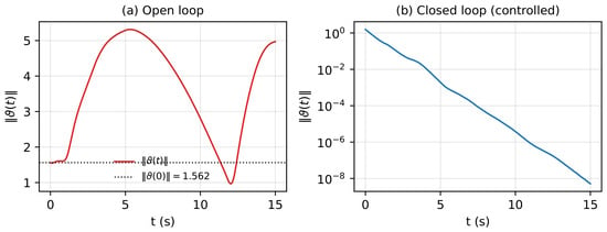
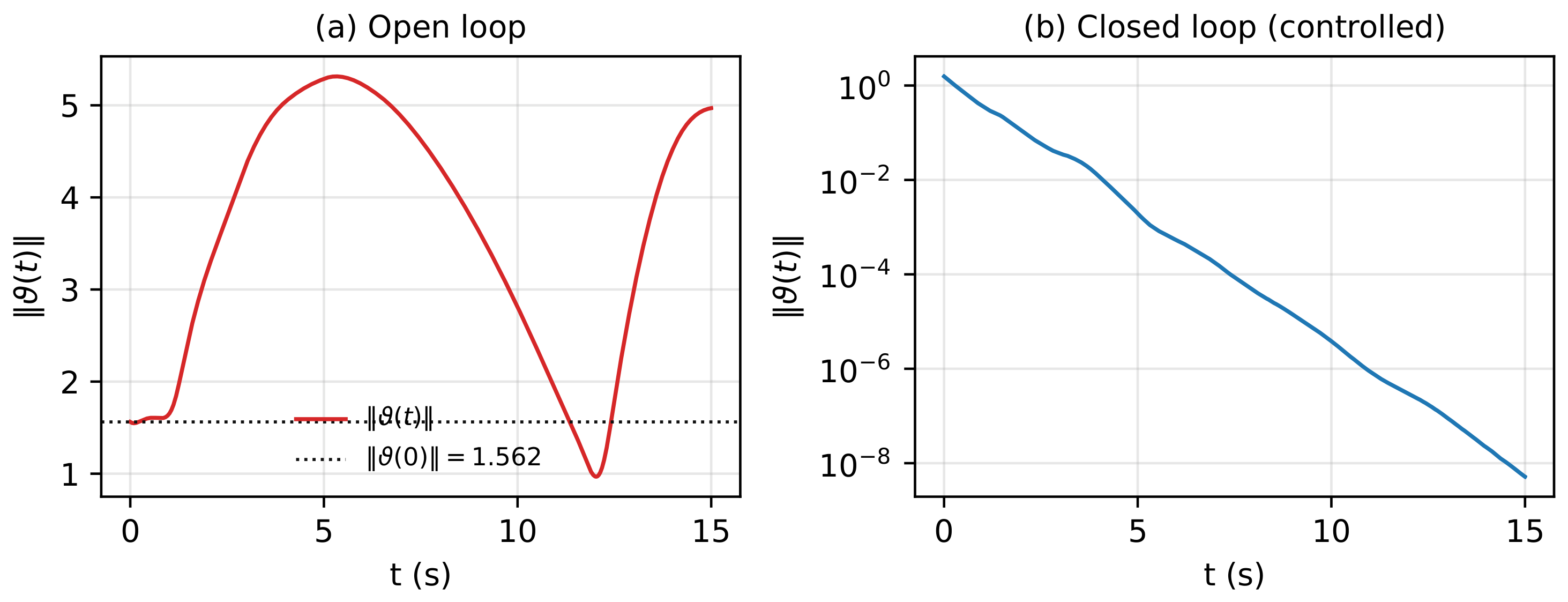
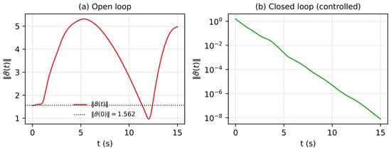
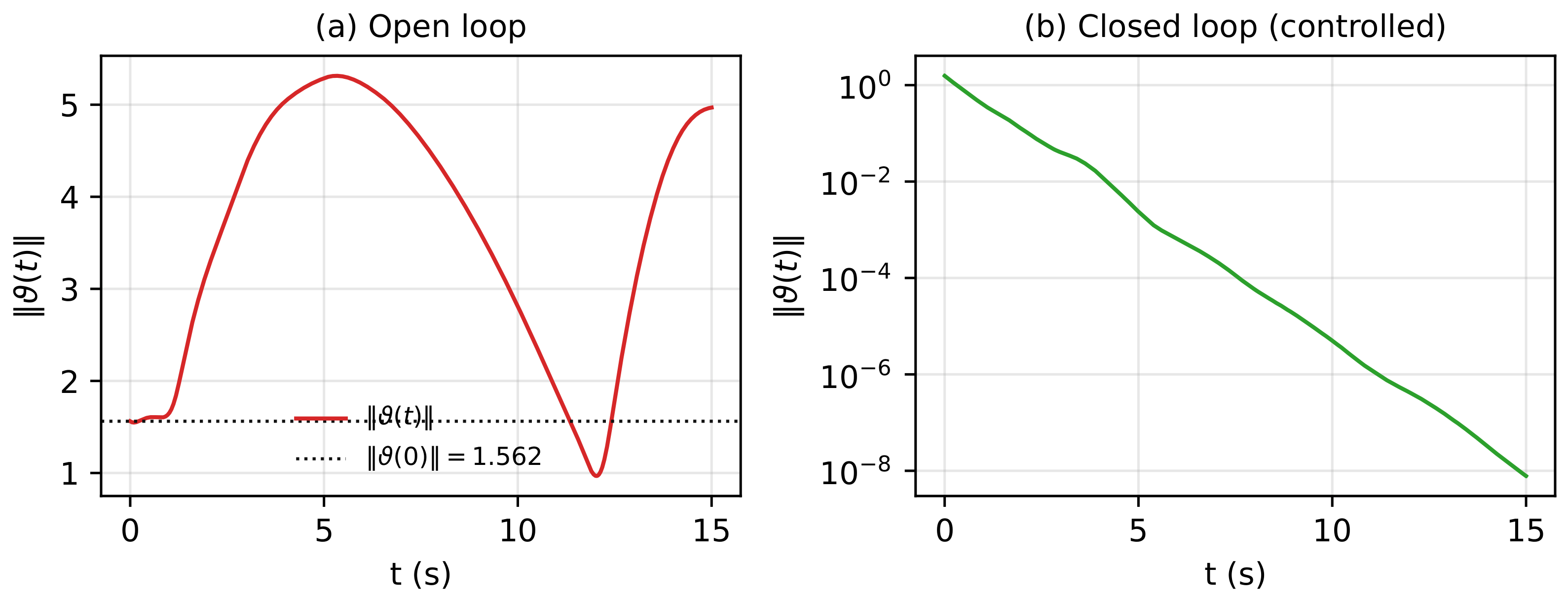
To confirm the design end to end, the closed-loop error system (4) with $A_l=0$, the gains of Table 2, and the sampling law (34) were simulated by explicit Euler integration with step ${10}^{-3}$ and initial error $\vartheta \left(0\right)=col\{1.2,-0.8,0.6\}$. Figure 1 shows that $\parallel \vartheta \left(t\right)\parallel$ decays monotonically below ${10}^{-8}$(final value $5.2\times {10}^{-9}$); the empirical log-decay rate on $[2,8]$ is $-1.35$, comfortably faster than the guaranteed rate $-\varrho /2=-0.0387$, reflecting the conservatism of the LKF-based bound. Without control, by contrast, the same error dynamics do not decay: Figure 1a shows $\parallel \vartheta \left(t\right)\parallel$ growing from $\parallel \vartheta \left(0\right)\parallel =1.562$ to a peak of about $5.31$ and then persisting, i.e., the origin of the open-loop error system is not asymptotically stable and the designed sampled-data controller is indispensable.

Figure 1. Example 1 (NNs): (a) open-loop evolution of $\parallel \vartheta \left(t\right)\parallel$ without control, showing that the error is amplified with respect to the initial value and persists; (b) evolution of $\parallel \vartheta \left(t\right)\parallel$ (semilog scale, blue curve) of the closed-loop error system under the stochastic sampling (34) with the gains of Table 2, decaying to the machine-precision level.

4.3. Example 2: Reaction–Diffusion Neural Networks

We now let the same network evolve over the one-dimensional domain $\mathsf{\Omega }=\{x\in \mathbb{R}:|x|\le 1\}$ ($m=1$, $L_1=2$, ${\lambda }_1={\pi }^2/4$) with diffusion coefficient matrix $A_1=0.05I_3$ and Dirichlet boundary condition $\vartheta (t,\pm 1)=0$; all other parameters, including the distribution (34), the decay parameters, and the delay, are as in Example 1. Hence the scalar checks (35) and the tail quantities are unchanged. Solving the truncated design LMI of Theorem 2 (S1) with the constraint $S{A}_1\ge 0$ yields the gains of Table 3 (status optimal, CLARABEL).

Table 3. Example 2 (RDNNs): redesigned gains $K_i=S^{-1}{Y}_i$, $i=1,\dots ,10$ under the revised LKF (all entries are new).

i	${\mathit{K}}_{\mathit{i}}$	i	${\mathit{K}}_{\mathit{i}}$
1	$\left[\begin{array}{ccc}-2.6067& 0.2136& 1.2113\\ -0.3478& -2.9249& -1.5831\\ 1.0312& -2.3251& -3.3951\end{array}\right]$	6	$\left[\begin{array}{ccc}-2.4554& 0.1368& 1.2726\\ -0.3410& -2.7258& -1.6424\\ 1.0339& -2.2272& -3.3592\end{array}\right]$
2	$\left[\begin{array}{ccc}-2.6347& 0.1753& 1.2540\\ -0.3504& -2.9501& -1.6273\\ 1.0389& -2.3116& -3.4822\end{array}\right]$	7	$\left[\begin{array}{ccc}-2.4564& 0.1350& 1.2747\\ -0.3411& -2.7259& -1.6450\\ 1.0343& -2.2258& -3.3636\end{array}\right]$
3	$\left[\begin{array}{ccc}-2.4487& 0.1506& 1.2575\\ -0.3401& -2.7252& -1.6235\\ 1.0319& -2.2391& -3.3275\end{array}\right]$	8	$\left[\begin{array}{ccc}-2.4571& 0.1337& 1.2763\\ -0.3412& -2.7260& -1.6470\\ 1.0345& -2.2247& -3.3669\end{array}\right]$
4	$\left[\begin{array}{ccc}-2.4521& 0.1434& 1.2651\\ -0.3406& -2.7254& -1.6330\\ 1.0328& -2.2328& -3.3435\end{array}\right]$	9	$\left[\begin{array}{ccc}-2.4577& 0.1327& 1.2775\\ -0.3412& -2.7261& -1.6485\\ 1.0348& -2.2240& -3.3694\end{array}\right]$
5	$\left[\begin{array}{ccc}-2.4541& 0.1394& 1.2696\\ -0.3408& -2.7256& -1.6386\\ 1.0334& -2.2294& -3.3530\end{array}\right]$	10	$\left[\begin{array}{ccc}-2.4581& 0.1319& 1.2785\\ -0.3412& -2.7262& -1.6497\\ 1.0349& -2.2233& -3.3714\end{array}\right]$

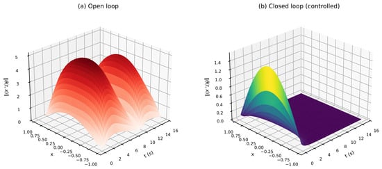
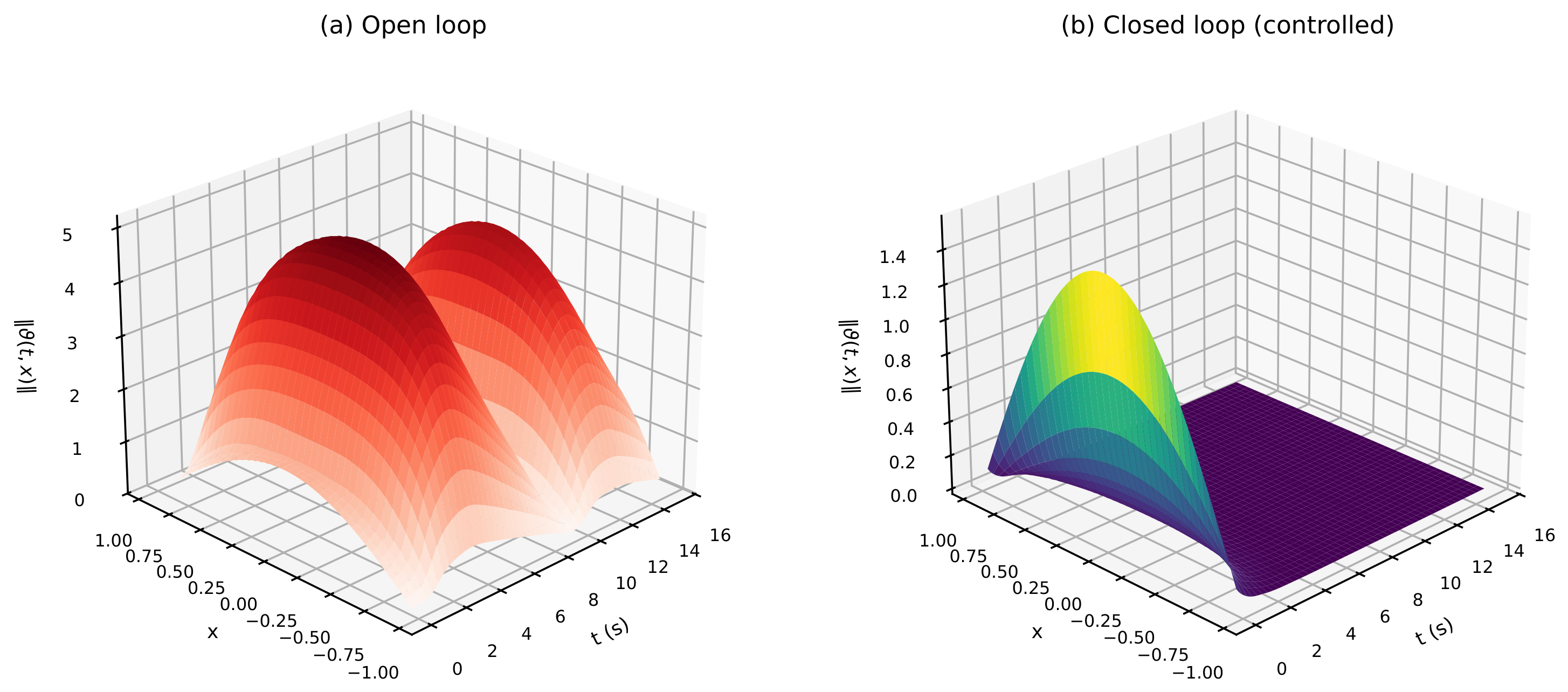
The tail verification (S2) is performed with $K_{\mathrm{tail}}=K_{10}$, $\rho =-0.02$, $\kappa =1$, and the diffusion constraint $S{A}_1\ge 0$; the analysis LMI is strictly feasible at both corner points $q=0.05$ and $q=0.054545$ in a single shared-variable problem, and ${max}_{p,q}|{\left[K_{10}\right]}_{pq}-{\left[K_9\right]}_{pq}|=2.0\times {10}^{-3}$. The reaction–diffusion system was discretized in space (41 grid points over $[-1,1]$, explicit Euler in time with step $5\times {10}^{-4}$) and simulated with the gains of Table 3 and the initial field $\vartheta (0,x)=cos(\pi x/2)col\{1.2,-0.8,0.6\}$. Figure 2 shows the space–time evolution of the pointwise error norm $\parallel \vartheta (t,x)\parallel$ as a three-dimensional surface; the corresponding $L^2$ norm decays below ${10}^{-8}$(final value $6.0\times {10}^{-9}$), again consistent with the theoretical almost-sure exponential decay. The open-loop reaction–diffusion error dynamics, simulated with the same parameters but with the control term removed, exhibit the same instability pattern: as shown in Figure 2a, the error norm surface grows from ${max}_x\parallel \vartheta (0,x)\parallel =1.562$ and the $L^2$ norm reaches a peak of about $5.11$ without returning to the origin. The contrast between the (a) and (b) panels of Figure 1 and Figure 2 demonstrates that the stabilization is due to the designed sampled-data controller rather than to the intrinsic dissipativity of the network.

Figure 2. Example 2 (RDNNs): three-dimensional surfaces of the pointwise error norm $\parallel \vartheta (t,x)\parallel$ over the space–time domain $(t,x)\in [0,15]\times [-1,1]$: (a) open-loop evolution without control, showing the same instability pattern; (b) closed-loop evolution of the reaction–diffusion error system with the gains of Table 3, decaying to the machine-precision level.

4.4. Example 3: General Parameter Sequences

Examples 1–2 use a piecewise-constant sequence ${\rho }_i$ that is non-positive for all $i\ge 3$. To demonstrate the framework beyond this case, we now take an NN with the same network data $B,I_3,C_1,C_2$ as in Example 1, the same delay, and the same activation, but with a varying decay sequence and a different geometric law. The sampling distribution is

$${\alpha }_i={\displaystyle \frac{1}{3}}{\left({\displaystyle \frac{2}{3}}\right)}^{i-1},q_i=0.05\left(1+{\displaystyle \frac{1}{i}}\right),i\ge 1,$$

(36)

so that ${\sum }_{i=1}^{\infty }{\alpha }_i=1$ and the tail mass has the closed form $\mathbb{P}\{h_k>q_N\}={(2/3)}^N$. The decay parameters are

$${\rho }_i=0.1-0.12\left(1-e^{-i/5}\right),i\ge 1,$$

(37)

which increase monotonically from ${\rho }_1=0.07825$ (so ${\rho }_0={\rho }_1$) through ${\rho }_5=0.02415$, ${\rho }_9=-0.00016$, and ${\rho }_{11}=-0.00670$, and converge to ${\rho }_{\infty }=-0.02$; thus the early modes have positive decay parameters and the tail modes are non-positive with ${\rho }_i\to -0.02$. All four regularity conditions hold: (C1)–(C2) by the geometric decay of ${\alpha }_i$, (C3) with the numerically computed truncated mean ${\overline{h}}_{10}=0.076530$ and the full-sequence averaged rate $\varrho =0.057107>0$ (see below), and (C4) with ${\rho }_0=0.07825$ and ${\delta }_0=e^{-2·0.07825·1.4}$.

Solving the truncated design LMI of Theorem 3 for $N=10$ yields the gains of Table 4 (status optimal, CLARABEL); the tail probability is ${(2/3)}^{10}=1.734\times {10}^{-2}$, and the truncated averaged rate is ${\varrho }_{10}=0.057930$, which matches the full averaged rate $\varrho =0.057107$ to within $1.4\%$. For the tail verification (S2), the tail parameters satisfy ${\rho }_i\in [{\rho }_{\infty },{\rho }_{11}]=[-0.02,-0.00670]$ for all $i>10$ (all non-positive), so Case A applies with the corner points $q\in \{0.05,0.054545\}$ and $\rho \in \{-0.00670,-0.02\}$; the shared-variable corner problem is strictly feasible (status optimal), certifying the analysis LMI for every $i>10$.

Table 4. Example 3 (NNs, general parameter sequences): designed gains $K_i=S^{-1}{Y}_i$, $i=1,\dots ,10$.

i	${\mathit{K}}_{\mathit{i}}$	i	${\mathit{K}}_{\mathit{i}}$
1	$\left[\begin{array}{ccc}-2.6591& 0.1528& 1.2213\\ -0.3614& -2.9520& -1.6078\\ 1.0276& -2.3103& -3.4504\end{array}\right]$	6	$\left[\begin{array}{ccc}-2.6048& 0.0823& 1.2837\\ -0.3589& -2.8646& -1.6764\\ 1.0388& -2.2452& -3.5001\end{array}\right]$
2	$\left[\begin{array}{ccc}-2.6592& 0.1108& 1.2585\\ -0.3615& -2.9408& -1.6457\\ 1.0362& -2.2848& -3.5031\end{array}\right]$	7	$\left[\begin{array}{ccc}-2.5957& 0.0802& 1.2850\\ -0.3583& -2.8530& -1.6778\\ 1.0389& -2.2408& -3.4944\end{array}\right]$
3	$\left[\begin{array}{ccc}-2.6439& 0.0966& 1.2724\\ -0.3610& -2.9170& -1.6630\\ 1.0377& -2.2685& -3.5143\end{array}\right]$	8	$\left[\begin{array}{ccc}-2.5881& 0.0786& 1.2858\\ -0.3578& -2.8435& -1.6787\\ 1.0389& -2.2373& -3.4895\end{array}\right]$
4	$\left[\begin{array}{ccc}-2.6289& 0.0895& 1.2785\\ -0.3603& -2.8961& -1.6704\\ 1.0384& -2.2582& -3.5119\end{array}\right]$	9	$\left[\begin{array}{ccc}-2.5820& 0.0773& 1.2865\\ -0.3574& -2.8358& -1.6794\\ 1.0389& -2.2345& -3.4854\end{array}\right]$
5	$\left[\begin{array}{ccc}-2.6158& 0.0852& 1.2818\\ -0.3596& -2.8788& -1.6742\\ 1.0387& -2.2508& -3.5062\end{array}\right]$	10	$\left[\begin{array}{ccc}-2.5769& 0.0764& 1.2870\\ -0.3571& -2.8294& -1.6800\\ 1.0390& -2.2322& -3.4819\end{array}\right]$

The closed-loop error system was simulated with the gains of Table 4 and the sampling law (36) (explicit Euler, step ${10}^{-3}$, initial error $\vartheta \left(0\right)=col\{1.2,-0.8,0.6\}$). Figure 3 shows that $\parallel \vartheta \left(t\right)\parallel$ again decays below ${10}^{-8}$ (final value $7.8\times {10}^{-9}$), with an empirical log-decay rate of $-1.32$ on $[2,8]$, faster than the guaranteed $-\varrho /2=-0.0286$; the open-loop error, with the control term removed, is amplified to a peak of about $5.31$ and persists, as in Example 1. The successive gains converge with ${max}_{p,q}|{\left[K_{10}\right]}_{pq}-{\left[K_9\right]}_{pq}|=6.3\times {10}^{-3}$, confirming that the tail gain $K_{\mathrm{tail}}=K_{10}$ is a consistent limit.

Figure 3. Example 3 (NNs, general parameter sequences): (a) open-loop evolution of $\parallel \vartheta \left(t\right)\parallel$ without control; (b) evolution of $\parallel \vartheta \left(t\right)\parallel$ (semilog scale, green curve) of the closed-loop error system under the sampling law (36) with the gains of Table 4, decaying to the machine-precision level.

4.5. Sensitivity of the Design with Respect to the Truncation Level N

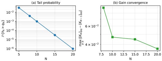
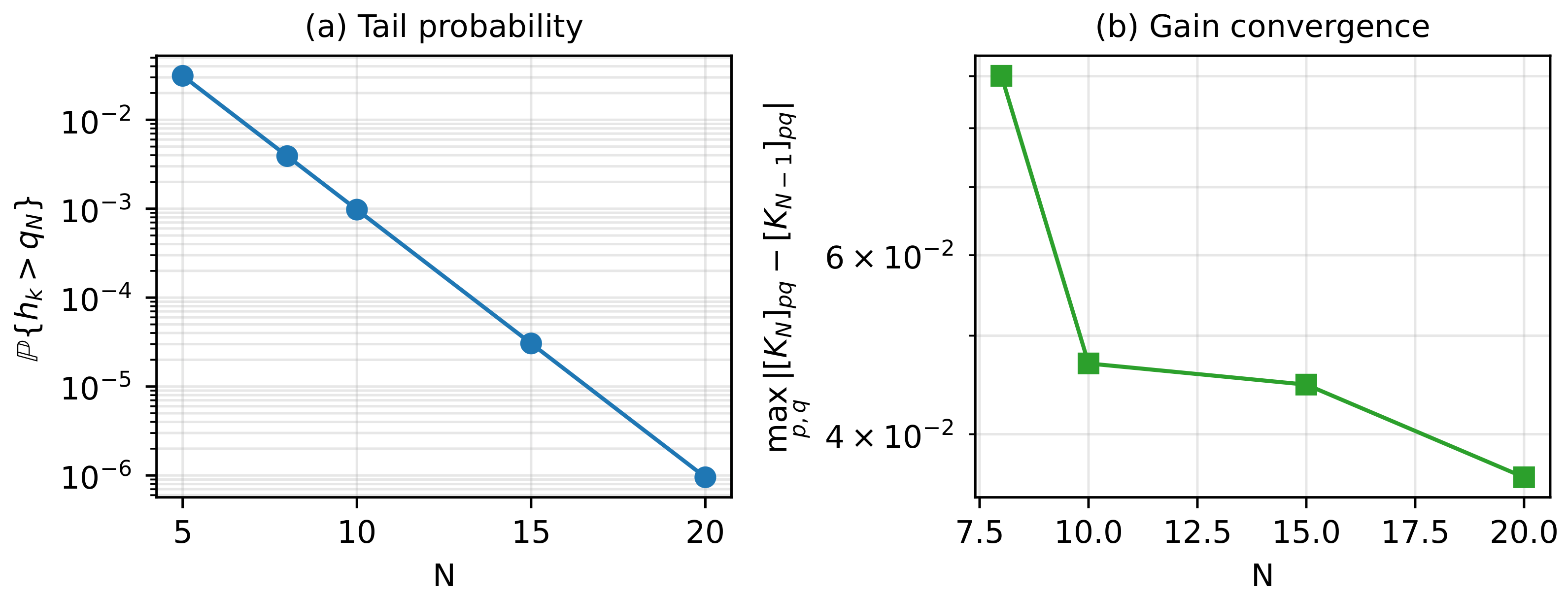
The truncation level N trades computational cost against the unverified tail mass $\mathbb{P}\{h_k>q_N\}$. Table 5 reports, for Example 1, the design at five truncation levels. In all cases the truncated design is feasible (optimal, CLARABEL) and the shared-variable tail verification (Case A) passes. The truncated averaged rate ${\varrho }_N$ decreases monotonically toward the full rate $\varrho =0.077452$: at $N=5$ it overshoots by $2.7\%$, while from $N=15$ onward it agrees with $\varrho$ to four significant digits. The gain increment ${max}_{p,q}|{\left[K_N\right]}_{pq}-{\left[K_{N-1}\right]}_{pq}|$ drops from $9.0\times {10}^{-2}$ at $N=8$ to $3.6\times {10}^{-2}$ at $N=20$, showing a clear convergence of the designed gains as the tail mass shrinks from $3.12\times {10}^{-2}$ ($N=5$) to $9.54\times {10}^{-7}$ ($N=20$). This confirms the practical guideline of (S2): if the tail verification failed for a given N, increasing N reduces the tail mass geometrically and eventually certifies the whole infinite family. Figure 4 visualizes the decay of the tail mass and of the gain increment with N.

Table 5. Sensitivity of the truncated design with respect to the truncation level N (Example 1).

N	$\mathbb{P}\{{\mathit{h}}_{\mathit{k}}>{\mathit{q}}_{\mathit{N}}\}$	${\mathit{\varrho }}_{\mathit{N}}$	Tail Verification	${max}_{\mathit{p},\mathit{q}}|{\left[{\mathit{K}}_{\mathit{N}}\right]}_{\mathit{pq}}-{\left[{\mathit{K}}_{\mathit{N}-1}\right]}_{\mathit{pq}}|$
5	$3.12\times {10}^{-2}$	$0.079560$	PASS	–
8	$3.91\times {10}^{-3}$	$0.077700$	PASS	$9.0\times {10}^{-2}$
10	$9.77\times {10}^{-4}$	$0.077513$	PASS	$4.7\times {10}^{-2}$
15	$3.05\times {10}^{-5}$	$0.077454$	PASS	$4.5\times {10}^{-2}$
20	$9.54\times {10}^{-7}$	$0.077452$	PASS	$3.6\times {10}^{-2}$

Figure 4. N-sensitivity analysis (Example 1): (a) tail mass $\mathbb{P}\{h_k>q_N\}=2^{-N}$ (log scale) and truncated averaged rate ${\varrho }_N$ versus N; (b) gain increment ${max}_{p,q}|{\left[K_N\right]}_{pq}-{\left[K_{N-1}\right]}_{pq}|$ versus N.

4.6. Comparison with a Fixed-Period Controller

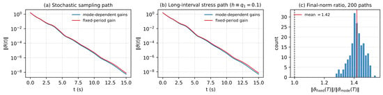
To quantify the benefit of the mode-dependent gains $K_{{\sigma }_k}$, we compare Example 1 with a fixed-period sampled-data controller whose sampling interval is the mean $h=\overline{h}=0.084657$ and whose constant gain is designed at the point $({\rho }^{★},{\kappa }^{★})=(\varrho ,\kappa )=(0.077454,1)$ of the averaged system. The fixed design is feasible (optimal, CLARABEL), yielding a constant gain; Table 1 places this comparison in context. The two controllers are simulated on the same stochastic sampling law (34) (explicit Euler, step ${10}^{-3}$, same initial error, 200 independent random paths of 3000 samples each). On the same random path realizing tail events, the mode-dependent controller attains a final error of $5.4\times {10}^{-9}$ versus $7.7\times {10}^{-9}$ for the fixed-period controller. Under a long-interval stress path ($h_k\equiv q_1=0.1$, the largest interval), the mode-dependent design reaches $4.6\times {10}^{-9}$ versus $7.0\times {10}^{-9}$. Over the 200-path Monte Carlo run, the mean final error of the mode-dependent controller is $5.4\times {10}^{-9}$ versus $7.7\times {10}^{-9}$ for the fixed one (about $30\%$ smaller), and no fixed-path peak exceeded $1.05$ times the corresponding mode-dependent peak. Figure 5 shows both controllers on the stochastic and stress paths and, in panel (c), the histogram of the final-error ratio over the 200 paths, whose mean is $1.42$: on every path the mode-dependent controller reaches a strictly smaller final error than the fixed-period one. The mode-dependent design thus remains competitive and, in particular, never underperforms the fixed-period design on the tested paths, which is consistent with its theoretical rate guarantee $\varrho /2$.

Figure 5. Comparison with a fixed-period controller (Example 1): (a) $\parallel \vartheta \left(t\right)\parallel$ (semilog scale) on a stochastic sampling path containing tail events; (b) $\parallel \vartheta \left(t\right)\parallel$ (semilog scale) on the long-interval stress path ($h\equiv q_1=0.1$), both under the mode-dependent and the fixed-period controllers; (c) histogram (blue bars) over 200 random paths of the ratio of the fixed-period final error to the mode-dependent final error (the red vertical line marks the mean $1.42$; no path falls below 1).

4.7. Discussion

Five observations are worth highlighting. First, the same infinite distribution and the same two-step procedure are applied to the NN, the RDNN, and the general parameter models, showing that the framework is model-agnostic: the diffusion term merely adds the constraint $S{A}_l\ge 0$ and a negative (dissipative) contribution to the LMI, and the decay sequence may be piecewise-constant (Examples 1 and 2) or smoothly varying with positive early modes (Example 3). Second, the guaranteed decay rate is an almost-sure quantity obtained from the strong-law argument: $\varrho =0.077452$ for Examples 1 and 2 (reproduced by the truncated design, ${\varrho }_{10}=0.077514$) and $\varrho =0.057107$ for Example 3 (${\varrho }_{10}=0.057930$); the observed simulation rates ($-1.35$ to $-1.32$) are 35–46 times faster, as expected from the conservatism of the LKF. Third, the tail verification is quantitative: with $N=10$ the unverified tail carries $9.766\times {10}^{-4}$ (Examples 1 and 2) or $1.734\times {10}^{-2}$ (Example 3) of the sampling probability, and it is certified by corner-point feasibility checks with shared variables (Case A), whose affine-in-parameter structure is established in (S2); the N-sensitivity analysis of Section 4.5 confirms that the truncated rate and the gains converge as the tail mass decays geometrically ($2^{-N}$ or ${(2/3)}^N$). Had the tail verification failed, one would simply increase N; for the geometric distributions used here, the truncation error vanishes geometrically. Fourth, the comparison of Section 4.6 shows that the mode-dependent design matches or improves on a fixed-period controller on the same stochastic sampling law, both on a stress path and over 200 random paths (about $30\%$ smaller mean final error). Fifth, the open-loop simulations of the (a) panels in Figure 1, Figure 2 and Figure 3 confirm that the exponential decay observed in the (b) panels is genuinely due to the sampled-data controller: without it, the synchronization error of all three models is amplified and never returns to the origin.

5. Conclusions

We generalized the stochastic sampled-data synchronization framework of [28] from finite to infinite discrete sampling distributions. Under four regularity conditions, almost-sure exponential synchronization of reaction–diffusion neural networks was established through a mode-dependent LKF that is continuous across sampling instants, with the probabilistic step strengthened from the weak law to a strong-law plus Cesàro argument and an explicit rate given by the probability-averaged decay parameter; synchronization in probability follows as a corollary. Design conditions were given in terms of LMIs, and a truncation-with-tail-verification procedure was proposed for the infinite LMI family: when the tail decay parameters are non-positive, the tail conditions are affine and certified by corner-point feasibility checks with shared variables; otherwise, a convergent-tail argument applies. The framework was validated on three numerical examples covering a neural network with a geometric sampling law, a reaction–diffusion neural network, and a general parameter model with a varying decay sequence; an N-sensitivity analysis confirmed the convergence of the truncated design, and a comparison with a fixed-period controller on 200 random paths showed the mode-dependent design to be at least as effective. Future work includes extending the framework to Markovian switching of the sampling law, to output-feedback protocols, and to distributions with heavy tails for which the mean (C1) fails; we note that for such heavy-tailed distributions, the tail certificate of (S2) must be revisited, since the affine structure of Case A rests on the boundedness assumptions (C1)–(C2).

References

- Hopfield, J.J. Neural networks and physical systems with emergent collective computational abilities. Proc. Natl. Acad. Sci. USA 1982, 79, 2554–2558. [Google Scholar] [CrossRef] [Scilit] [PubMed]
- Chua, L.O.; Yang, L. Cellular neural networks: Applications. IEEE Trans. Circuits Syst. 1988, 35, 1273–1290. [Google Scholar] [CrossRef] [Scilit]
- Zhang, Z.M.; He, Y.; Wu, M.; Wang, Q.-G. Exponential synchronization of neural networks with time-varying delays via dynamic intermittent output feedback control. IEEE Trans. Syst. Man Cybern. Syst. 2019, 49, 612–622. [Google Scholar] [CrossRef] [Scilit]
- Xiao, J.; Zhong, S.; Wen, S. Unified analysis on the global dissipativity and stability of fractional-order multidimension-valued memristive neural networks with time delay. IEEE Trans. Neural Netw. Learn. Syst. 2022, 33, 5656–5665. [Google Scholar] [CrossRef] [Scilit] [PubMed]
- Wang, L.; Zeng, Z.; Ge, M. A disturbance rejection framework for finite-time and fixed-time stabilization of delayed memristive neural networks. IEEE Trans. Syst. Man Cybern. Syst. 2021, 51, 905–915. [Google Scholar] [CrossRef] [Scilit]
- Turing, A.M. The chemical basis of morphogenesis. Philos. Trans. R. Soc. B 1952, 237, 37–72. [Google Scholar] [CrossRef] [Scilit]
- Chen, W.; Luo, S.; Zheng, W.X. Impulsive synchronization of reaction-diffusion neural networks with mixed delays and its application to image encryption. IEEE Trans. Neural Netw. Learn. Syst. 2016, 27, 2696–2710. [Google Scholar] [CrossRef] [Scilit] [PubMed]
- Sheng, Y.; Zeng, Z. Impulsive synchronization of stochastic reaction-diffusion neural networks with mixed time delays. Neural Netw. 2018, 103, 83–93. [Google Scholar] [CrossRef] [Scilit] [PubMed]
- Zhang, R.; Wang, H.; Park, J.H.; Lam, H.K.; He, P. Quasi-synchronization of reaction-diffusion neural networks under deception attacks. IEEE Trans. Syst. Man Cybern. Syst. 2022, 52, 7833–7844. [Google Scholar] [CrossRef] [Scilit]
- Zhang, R.; Zeng, D.; Park, J.H.; Liu, Y.; Xie, X. Adaptive event-triggered synchronization of reaction-diffusion neural networks. IEEE Trans. Neural Netw. Learn. Syst. 2021, 32, 3723–3735. [Google Scholar] [CrossRef] [Scilit] [PubMed]
- Zhang, R.; Zeng, D.; Park, J.H.; Lam, H.K.; Zhou, S. Fuzzy adaptive event-triggered sampled-data control for stabilization of T-S fuzzy memristive neural networks with reaction-diffusion terms. IEEE Trans. Fuzzy Syst. 2021, 29, 1775–1785. [Google Scholar] [CrossRef] [Scilit]
- Wu, Y.; Liu, L.; Hu, J.; Feng, G. Adaptive antisynchronization of multi-layer reaction-diffusion neural networks. IEEE Trans. Neural Netw. Learn. Syst. 2018, 29, 807–818. [Google Scholar] [CrossRef] [Scilit] [PubMed]
- Guo, Z.; Wang, S.; Wang, J. Global exponential synchronization of coupled delayed memristive neural networks with reaction-diffusion terms via distributed pinning controls. IEEE Trans. Neural Netw. Learn. Syst. 2021, 32, 105–116. [Google Scholar] [CrossRef] [Scilit] [PubMed]
- Rao, R.; Zhu, Q. Synchronization for reaction–diffusion switched delayed feedback epidemic systems via impulsive control. Mathematics 2024, 12, 447. [Google Scholar] [CrossRef] [Scilit]
- Zeng, D.; Zhang, R.; Park, J.H.; Pu, Z.; Liu, Y. Pinning synchronization of directed coupled reaction-diffusion neural networks with sampled-data communications. IEEE Trans. Neural Netw. Learn. Syst. 2020, 31, 2092–2103. [Google Scholar] [CrossRef] [Scilit] [PubMed]
- Chen, G.; Xia, J.; Park, J.H.; Shen, H.; Zhuang, G. Asynchronous sampled-data controller design for switched Markov jump systems and its applications. IEEE Trans. Syst. Man Cybern. Syst. 2023, 53, 934–946. [Google Scholar] [CrossRef] [Scilit]
- Wang, X.; Park, J.H.; Yang, H.; Zhao, G.; Zhong, S. An improved fuzzy sampled-data control to stabilization of T-S fuzzy systems with state delays. IEEE Trans. Cybern. 2020, 50, 3125–3135. [Google Scholar] [CrossRef] [Scilit] [PubMed]
- Lu, B.; Jiang, H.; Hu, C.; Abdurahman, A. Spatial sampled-data control for H∞ output synchronization of directed coupled reaction-diffusion neural networks with mixed delays. Neural Netw. 2020, 123, 429–440. [Google Scholar] [CrossRef] [Scilit] [PubMed]
- Zhang, R.; Zeng, D.; Park, J.H.; Lam, H.K.; Xie, X. Fuzzy sampled-data control for synchronization of T-S fuzzy reaction-diffusion neural networks with additive time-varying delays. IEEE Trans. Cybern. 2021, 51, 2384–2397. [Google Scholar] [CrossRef] [Scilit] [PubMed]
- Chen, S.; Lim, C.-C.; Shi, P.; Lu, Z. Synchronization control for reaction-diffusion FitzHugh-Nagumo systems with spatial sampled-data. Automatica 2018, 93, 352–362. [Google Scholar] [CrossRef] [Scilit]
- Wang, Z.P.; Wu, H.N.; Wang, J.L.; Li, H.X. Quantized sampled-data synchronization of delayed reaction-diffusion neural networks under spatially point measurements. IEEE Trans. Cybern. 2021, 51, 5740–5751. [Google Scholar] [CrossRef] [Scilit] [PubMed]
- Gao, H.; Wu, J.; Shi, P. Robust sampled-data H∞ control with stochastic sampling. Automatica 2009, 45, 1729–1736. [Google Scholar] [CrossRef] [Scilit]
- Shen, B.; Wang, Z.; Liu, X. Sampled-data synchronization control of dynamical networks with stochastic sampling. IEEE Trans. Autom. Control 2012, 57, 2644–2650. [Google Scholar] [CrossRef] [Scilit]
- He, W.; Zhang, B.; Han, Q.-L.; Qian, F.; Kurths, J.; Cao, J. Leader-following consensus of nonlinear multiagent systems with stochastic sampling. IEEE Trans. Cybern. 2017, 47, 327–338. [Google Scholar] [CrossRef] [Scilit] [PubMed]
- Du, S.-L.; Xia, W.; Ren, W.; Sun, X.-M.; Wang, W. Observer-based consensus for multiagent systems under stochastic sampling mechanism. IEEE Trans. Syst. Man Cybern. Syst. 2018, 48, 2328–2338. [Google Scholar] [CrossRef] [Scilit]
- Su, H.; Zhang, J.; Chen, X. A stochastic sampling mechanism for time-varying formation of multiagent systems with multiple leaders and communication delays. IEEE Trans. Neural Netw. Learn. Syst. 2019, 30, 3699–3707. [Google Scholar] [CrossRef] [Scilit] [PubMed]
- Rakkiyappan, R.; Dharani, S.; Cao, J. Synchronization of neural networks with control packet loss and time-varying delay via stochastic sampled-data controller. IEEE Trans. Neural Netw. Learn. Syst. 2015, 26, 3215–3226. [Google Scholar] [CrossRef] [Scilit] [PubMed]
- Zeng, D.; Yang, L.; Zhang, R.; Park, J.H.; Pu, Z.; Xie, X. A new switching system protocol for synchronization in probability of RDNNs with stochastic sampling. IEEE Trans. Syst. Man Cybern. Syst. 2023, 53, 4358–4369. [Google Scholar] [CrossRef] [Scilit]
- Thomas, J.; Steur, E.; Fiter, C.; Hetel, L.; van de Wouw, N. Exponential synchronization of networked systems under asynchronous sampled-data coupling. Automatica 2025, 175, 112157. [Google Scholar] [CrossRef] [Scilit]
- Zhang, X.-M.; Han, Q.-L.; Zhang, B.-L.; Ge, X.; Zhang, D. Accumulated-state-error-based event-triggered sampling scheme and its application to H∞ control of sampled-data systems. Sci. China Inf. Sci. 2024, 67, 162206. [Google Scholar] [CrossRef] [Scilit]
- Chen, P.; Zeng, H.; Xu, C. Exponential synchronization of reaction-diffusion neural networks via asynchronous sampled-data event-triggered control. Electron. Res. Arch. 2026, 34, 7244–7260. [Google Scholar] [CrossRef] [Scilit]
- Aili, A.; Chen, S.; Zhang, S. Event-triggered synchronization of coupled neural networks with reaction-diffusion terms. Mathematics 2024, 12, 1409. [Google Scholar] [CrossRef] [Scilit]
- Zhang, G.; Song, Y.; Liu, X. Exponential synchronization of coupled neural networks with hybrid delays and stochastic distributed delayed impulses. Mathematics 2024, 12, 1995. [Google Scholar] [CrossRef] [Scilit]
- Liao, W.-Q.; Zeng, H.-B.; Xiao, H.-Q.; Liang, J.-M. Synchronized control of chaotic neural networks with actuator saturation. IEEE Access 2024, 12, 73599–73607. [Google Scholar] [CrossRef] [Scilit]
- Kolmanovskii, V.; Myshkis, A. Introduction to the Theory and Applications of Functional Differential Equations; Kluwer Academic Publishers: Dordrecht, The Netherlands, 1999. [Google Scholar]
- Seuret, A.; Gouaisbaut, F. Wirtinger-based integral inequality: Application to time-delay systems. Automatica 2013, 49, 2860–2866. [Google Scholar] [CrossRef] [Scilit]
Disclaimer/Publisher’s Note: The statements, opinions and data contained in all publications are solely those of the individual author(s) and contributor(s) and not of MDPI and/or the editor(s). MDPI and/or the editor(s) disclaim responsibility for any injury to people or property resulting from any ideas, methods, instructions or products referred to in the content. |
© 2026 by the author. Licensee MDPI, Basel, Switzerland. This article is an open access article distributed under the terms and conditions of the Creative Commons Attribution (CC BY) license.