Analytical and Numerical Analysis of Time-Delayed NDF Control for Nonlinear Rotating Pendulums with Stiffness Modulation Under Simultaneous Resonance Conditions

Abstract

In this paper, the nonlinear dynamics and vibration suppression of a harmonically excited rotating pendulum are studied by a novel bidirectional coupled second-order auxiliary negative derivative feedback (NDF) controller. The governing equations are obtained by Lagrangian mechanics, extended to the case of quintic nonlinearities, for which the variable torsional stiffness is the nonlinear restoring torque. A unique feature of the proposed control configuration is the addition of two separate time-delay parameters in the bidirectional coupling, which allows us to investigate the effects of delayed interactions between the primary system and the auxiliary controller. The resulting coupled nonlinear system is analytically investigated by the averaging method under the simultaneous resonance conditions and the steady-state response and stability characteristics are obtained by the eigenvalue analysis. The analytical predictions are validated with direct numerical simulations by the fourth-order Runge–Kutta method. It is shown that the analytical predictions are effective at vibration suppression and the analytical and numerical responses are in good agreement. Furthermore, a detailed parametric study is presented to investigate the effects of the dual time delays, control gains, controller damping, and excitation amplitude on the nonlinear response and stability. The proposed framework thus integrates a bidirectional coupled second-order auxiliary NDF controller, dual time-delay effects, quintic nonlinear dynamics and simultaneous-resonance analysis into a unified vibration-control strategy.

1. Introduction

The rotating pendulum is a paradigmatic nonlinear dynamical system and has attracted much attention because of its extensive dynamics and its relevance for a broad class of mechanical and engineering problems. The first works in this direction are due to Crawford [1], who reported experimental results on the motion of a rotating pendulum. Additional studies [2] demonstrated the effectiveness of the pendulum systems in studying nonlinear oscillations, rotational dynamics, and complex responses. The pendulum mechanisms are fundamental in nonlinear dynamics but have also been used in advanced mechanical and precision sensing applications, showing their practical importance [3]. Rotating pendulum systems inherently exhibit nonlinear coupling between the rotational and angular motions, which results in a variety of dynamical regimes including small- and large-amplitude oscillations, periodic rotations, quasiperiodic responses, and chaotic motions. The rotating pendulums with these features are excellent benchmark systems for the study of nonlinear phenomena such as the resonance, stability, bifurcation and transitions between different modes of motion. From an engineering point of view, large-amplitude and resonant oscillations are generally not desirable because they can cause excessive vibration, reduced dynamic stability and degradation of system performance. Hence, vibration suppression has become an important subject of research in nonlinear mechanical systems. Different passive, semi-active and active control techniques have been developed to reduce undesirable vibrations and improve the stability of the system. Passive techniques, such as viscous damping and vibration absorbers, are structurally simple and reliable, but their effectiveness can be limited by varying operating conditions. Active control strategies use feedback measurements and actuators to modify the system dynamics in real time, which have the advantages of better adaptability and vibration-suppression capability [4,5,6]. However, the control of nonlinear systems is not always effective, as the system response may be strongly influenced by nonlinearities, external or parametric excitation, resonance and bifurcation. Therefore, proper control strategies are needed to reduce the vibrations and to maintain the desired dynamic features and stability of the system. Negative derivative feedback (NDF) is an appealing active feedback-control strategy because it directly tunes the velocity-dependent dynamics of the system. In a conventional NDF scheme, the control input is proportional to the negative time derivative of the measured displacement or angular response to change the effective damping and dissipate the vibrational energy. Thanks to its comparatively simple structure, easy implementation and relative few control parameters, the NDF is particularly suitable for nonlinear mechanical systems under resonant excitation. Recent work has demonstrated the effectiveness of NDF in a variety of non-linear systems. Jamshidi and Collette [7] proposed an optimal NDF controller for collocated systems by using H₂ and H_∞ optimization methods, and gave a systematic framework for vibration attenuation and robust controller design. Amer et al. [8] investigated NDF-based vibration suppression in smooth and discontinuous nonlinear oscillator and showed its effectiveness in damping nonlinear vibrations. Bauomy et al. [9] investigated NDF control and bifurcation behaviors in a two-degree-of-freedom coupled dynamical system with the influence of feedback on the stability of the system and its nonlinear responses. Most recently, El-Sayed et al. [10] investigated the NDF control of a nonlinear electromechanical oscillator under primary resonance and showed its effectiveness in enhancing stability and reducing resonance-induced vibrations. These studies show NDF is an effective active-control technique for vibration suppression and stability improvement in nonlinear dynamical systems. In real feedback control systems, time delay may be present in sensing, signal transmission, computational processing and actuator dynamics and can have a profound effect on the system response. It has been demonstrated that delayed feedback affects nonlinear oscillations and bifurcation behavior [11,12], active vibration control and stability [13,14], and vibration suppression in vehicle and flexible-structure systems [15,16]. Position- and velocity-dependent time-delay feedback was later shown to be effective for vibration suppression of a nonlinear oscillator by Amer et al. [17]. These studies show that even small delays may cause phase shifts and change the stability and vibration behavior of controlled systems. Alluhydan and Abd El-Salam [18] studied the vibration suppression and Hopf bifurcation control of a nonlinear rotating pendulum using time-delayed acceleration feedback. Their results confirmed the important influence of the delayed feedback on the stability and dynamic features of the rotating pendulum and demonstrated its applicability for the suppression of undesired oscillations. Although the NDF and time-delay vibration control have been developed [7,8,9,10,11,12,13,14,15,16,17,18], the combined effects of a bidirectional coupled second-order auxiliary NDF controller, dual time delays and higher-order nonlinearities are not sufficiently explored. Most of the previous works deal with the traditional NDF configurations or single-delay feedback, and their interaction with the quintic nonlinearities under simultaneous resonance has been little studied. In this study, a quintic nonlinear model of a rotating pendulum is proposed to fill these gaps, which is controlled by a bidirectional coupled second-order auxiliary NDF controller with two independent time delays. The steady-state response is obtained by the averaging method under simultaneous resonance; stability is studied by eigenvalue analysis and numerical simulations, and the analytical results are validated. The effects of dual delays, control parameters and excitation amplitude on vibration suppression are systemically investigated.

2. Description of the Rotating Pendulum Model

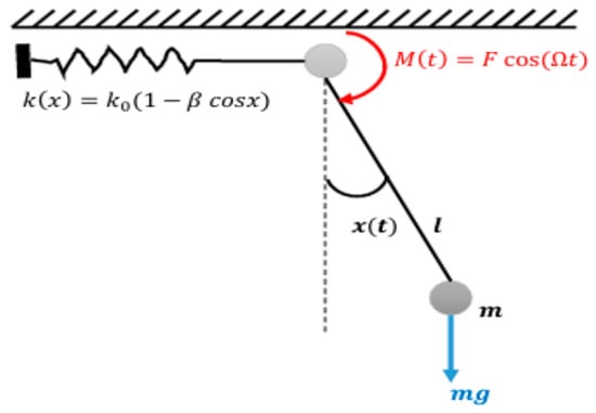
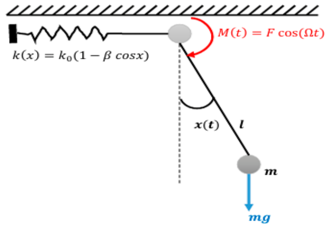
A rigid pendulum of length l and mass m is hinged at a fixed pivot. The system is subjected to gravitation force, and a harmonic force and a harmonic excitation torque f cosΩt are applied at the pivot. Additionally, a nonlinear torsional stiffness is introduced such that the restoring torque depends on the angular displacement as k(x) = k₀(1 − β cosx), leading to a modulated restoring force as shown in Figure 1. The nonlinear stiffness k(x) = k₀(1 − β cosx) models an angle-dependent restoring torque arising from geometric and elastic nonlinearities at the pendulum pivot. Such nonlinear behavior occurs in torsional elastic joints, compliant mechanisms, and nonlinear vibration absorbers, where the effective stiffness varies with angular displacement, while β controls the degree of nonlinearity.

Figure 1. Schematic model of the rotating pendulum.

The dynamics of a nonlinear rotating pendulum are derived using Lagrangian mechanics. The kinetic energy of the pendulum is given by

$$T={\displaystyle \frac{1}{2}}m{l}^2{\dot{x}}^2$$

(1)

To account for the nonlinear restoring effect, the potential energy is assumed in a modified form such that the restoring torque becomes (1 − β cosx)sinx. This is obtained by defining the potential energy as

$$V(x)=-\cos x-{\displaystyle \frac{\beta }{2}}{\sin }^{2}x$$

(2)

The Lagrangian formulation provides a systematic and convenient framework for deriving the governing equations of motion of the proposed dynamical system. Accordingly, by defining the kinetic and potential energies of the system in terms of the selected generalized coordinates, the Lagrangian function is constructed as the difference between the total kinetic energy and the total potential energy. Thus, the Lagrangian of the system is expressed as

$$L(x)=T(x)-V(x)={\displaystyle \frac{1}{2}}m{l}^2{\dot{x}}^2+\cos x+{\displaystyle \frac{\beta }{2}}{\sin }^{2}x$$

(3)

Applying the Euler–Lagrange equations to the system Lagrangian yields the governing equations of motion as follows:

$${\displaystyle \frac{d}{\mathit{dt}}}\left({\displaystyle \frac{\partial L}{\partial \dot{x}}}\right)-{\displaystyle \frac{\partial L}{\partial x}}=Q$$

(4)

Here, Q denotes the generalized external force, defined as

Q = F cos(Ω t)

(5)

where F and Ω represent the excitation amplitude and excitation frequency, respectively. Substituting the above expression into the Euler–Lagrange equation (4) and simplifying the resulting terms, the governing equation of motion can be obtained in the following form:

$${ml}^2\ddot{x}+\left(1-\beta \cos x\right)\sin x=F\cos (\mathsf{\Omega }\mathrm{t})$$

(6)

Dividing by ml² yields a normalized form in which the inertial coefficient is unity. The forcing amplitude is rescaled as f = F/ml². The equation of motion can be written in dimensionless form as

$$\ddot{x}+\left(1-\beta \cos x\right)\sin x=f\cos (\mathsf{\Omega }\mathrm{t})$$

(7)

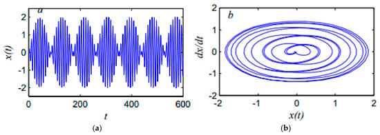
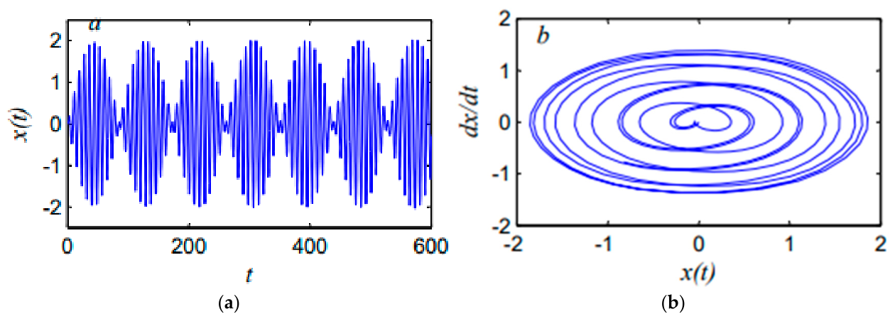
If β = 0, it reduces to the standard forced pendulum. The term (1 − βcosx) introduces additional nonlinearity, making the system closer to a Duffing-type or parametrically exited pendulum. This kind of equation can show multiple equilibria, bifurcations and possible chaotic behavior. Numerically, the fourth-order Runge–Kutta method was used to extract the numerical solutions of the uncontrolled rotating pendulum, as shown in Figure 2. This figure presents the time history and phase plane of the uncontrolled system. The time response shows sustained oscillations with nearly constant amplitude (about 2), indicating the absence of damping or control. The phase plane exhibits a closed orbit, confirming periodic motion and energy conservation in the system. This behavior highlights the necessity of introducing a control to suppress the vibrations. Therefore, time delay control was used with the negative derivative feedback (NDF) controller to suppress the rotating pendulum’s vibrations.

Figure 2. (a) The time history and (b) phase plane of uncontrolled system at primary resonance (Ω ≈ ω₁).

3. Mathematical Modeling of the Closed-Loop System

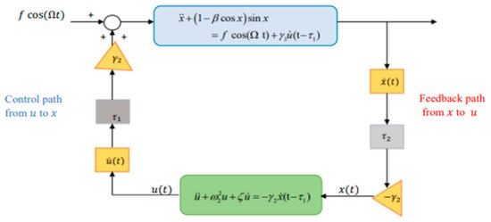
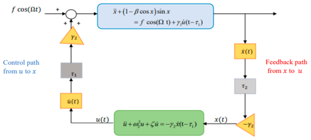
To scrutinize the dynamic behavior of the rotating pendulum after using a time delay with an NDF controller, the closed-loop system is worked out mathematically. The closed loop system consists of a nonlinear rotating pendulum coupled with a secondary damped NDF controller. A delayed negative derivative feedback control strategy is implemented through bidirectional coupling between the main system and the NDF controller as shown in Figure 3. Equation (7) can be written as

$$\ddot{x}+\left(1-\beta \cos x\right)\sin x=f\cos (\mathsf{\Omega }\mathrm{t})+{\mathrm{F}}_c(t)$$

(8)

$$\ddot{u}+{\omega }_2^{2}u+\zeta \dot{u}={\mathrm{F}}_f(t)$$

(9)

where ${\mathrm{F}}_c(t)={\gamma }_1\dot{u}(t-{\tau }_1)$ is the control signal and ${\mathrm{F}}_f(t)=-{\gamma }_2\dot{x}(t-{\tau }_2)$ is the feedback signal. According to the Maclaurin series, sinxand cosx are

$$\left.\begin{array}{l}\sin x=x-{\displaystyle \frac{x^3}{6}}+\dots \\ \cos x=1-{\displaystyle \frac{x^2}{2}}+\dots \end{array}\right\}$$

(10)

Figure 3. Closed-loop diagram of the controlled rotating pendulum system with time-delayed derivative feedback controller.

The trigonometric terms are related to the original physical nonlinearities of the pendulum system. The Maclaurin expansion is introduced to obtain a polynomial form suitable for analytical treatment. The dominant nonlinear effects are retained by keeping terms up to fifth order, while preserving mathematical tractability. For the range of angular motion considered, higher-order terms make negligible contributions, while truncations of lower order may reduce the accuracy of the nonlinear response. Numerical comparison with the original trigonometric functions demonstrates that the fifth-order approximation provides sufficient accuracy in the investigated displacement range. Equations (8) and (9) can be written as

$$\ddot{x}+{\omega }_1^{2}x+{\delta }_1{x}^3-{\delta }_2{x}^5=f\cos \mathsf{\Omega }t+{\gamma }_1\dot{u}(\mathrm{t}-{\tau }_1)$$

(11)

$$\ddot{u}+{\omega }_2^{2}u+\zeta \dot{u}=-{\gamma }_2\dot{x}(t-{\tau }_2)$$

(12)

where ${\omega }_1=\sqrt{1-\beta },{\delta }_1={\displaystyle \frac{4\beta -1}{6}}$ and ${\delta }_2={\displaystyle \frac{\beta }{12}}$.

3.1. The Method of Averaging

The method of averaging is a classical perturbation method widely used to analyze weakly nonlinear dynamical systems with periodic responses. In the present study the method is used under the assumption of weak nonlinearity, small external excitation and slowly varying amplitudes and phases. The governing equations are averaged over an oscillation period to remove the fast-time variations, yielding reduced slow-flow equations which describe the essential system dynamics and allow the analysis of steady-state responses, resonance behavior and stability. The application of the averaging method follows the standard procedure outlined in [19]. To obtain the approximate solutions of Equations (11) and (12), we will use the average method as follows:

$$\left.\begin{array}{l}x(\mathrm{t})={\mathrm{a}}_1\cos \left({\omega }_{1}t+{\theta }_1\right),\\ u(\mathrm{t})={\mathrm{a}}_2\cos \left({\omega }_{2}t+{\theta }_2\right)\end{array}\right\}$$

(13)

where a_i and θ_i (i = 1,2) are constants to set the unperturbed harmonic solution. Then, according to the averaging method, they may slowly vary with time. The first and second time derivatives are then obtained by differentiating the corresponding expression in relation to time (t) and they yield

$$\left.\begin{array}{l}\dot{x}(\mathrm{t})=-{\omega }_1{\mathrm{a}}_1\sin \left({\omega }_{1}t+{\theta }_1\right),\\ \dot{u}(\mathrm{t})=-{\omega }_2{\mathrm{a}}_2\sin \left({\omega }_{2}t+{\theta }_2\right)\end{array}\right\}$$

(14)

$$\left.\begin{array}{l}\dot{x}(\mathrm{t}-{\tau }_2)=-{\omega }_1{\mathrm{a}}_1\sin \left({\omega }_{1}t-{\omega }_1{\tau }_2+{\theta }_1\right),\\ \dot{u}(\mathrm{t}-{\tau }_1)=-{\omega }_2{\mathrm{a}}_2\sin \left({\omega }_{2}t-{\omega }_2{\tau }_1+{\theta }_2\right)\end{array}\right\}$$

(15)

$$\left.\begin{array}{l}\ddot{x}(\mathrm{t})=-{\omega }_1^2{\mathrm{a}}_1\cos \left({\omega }_{1}t+{\theta }_1\right),\\ \ddot{u}(\mathrm{t})=-{\omega }_2^2{\mathrm{a}}_2\cos \left({\omega }_{2}t+{\theta }_2\right)\end{array}\right\}$$

(16)

where a_i and θ_i (i = 1,2) denote the amplitudes and phases associated with the main system and the control input, respectively. The solutions of Equations (11) and (12) are assumed in the form given by Equation (13), subject to the constraint specified in Equation (14). Since the amplitudes and phases are time-dependent quantities, differentiating Equation (14) with respect to time (t) yields the following relation:

$$\left.\begin{array}{l}\dot{x}(\mathrm{t})={\dot{\mathrm{a}}}_1\cos \left({\omega }_{1}t+{\theta }_1\right)-{\mathrm{a}}_1{\dot{\theta }}_1\sin \left({\omega }_{1}t+{\theta }_1\right)-{\mathrm{a}}_1{\omega }_1\sin \left({\omega }_{1}t+{\theta }_1\right),\\ \dot{u}(\mathrm{t})={\dot{\mathrm{a}}}_2\cos \left({\omega }_{2}t+{\theta }_2\right)-{\mathrm{a}}_2{\dot{\theta }}_2\sin \left({\omega }_{2}t+{\theta }_2\right)-{\mathrm{a}}_2{\omega }_2\sin \left({\omega }_{2}t+{\theta }_2\right)\end{array}\right\}$$

(17)

By comparing Equations (14) and (17), and carefully matching the corresponding terms, the following set of relations is obtained:

$${\dot{\mathrm{a}}}_1\cos \left({\omega }_{1}t+{\theta }_1\right)-{\mathrm{a}}_1{\dot{\theta }}_1\sin \left({\omega }_{1}t+{\theta }_1\right)=0$$

(18a)

$${\dot{\mathrm{a}}}_2\cos \left({\omega }_{2}t+{\theta }_2\right)-{\mathrm{a}}_2{\dot{\theta }}_2\sin \left({\omega }_{2}t+{\theta }_2\right)=0$$

(18b)

Differentiating Equation (14) once again with respect to time (t), we obtain the following relations:

$$\left.\begin{array}{l}\ddot{x}+{\omega }_1^{2}x=-{\omega }_1{\dot{a}}_1\sin ({\omega }_{1}t+{\theta }_1)-{\omega }_1{a}_1{\dot{\theta }}_1\cos ({\omega }_{1}t+{\theta }_1)\\ \ddot{u}+{\omega }_2^{2}u=-{\omega }_2{\dot{a}}_2\sin ({\omega }_{2}t+{\theta }_2)-{\omega }_2{a}_2{\dot{\theta }}_2\cos ({\omega }_{2}t+{\theta }_2)\end{array}\right\}$$

(19)

Inserting Equations (13) and (14) in Equations (11) and (12) results in the following:

$$\ddot{x}+{\omega }_1^{2}x=f\cos \mathsf{\Omega }t-{\omega }_2{\gamma }_1{a}_2\sin ({\omega }_{2}t+{\theta }_2-{\omega }_2{\tau }_1)-{\delta }_1{a}_1^3{\cos }^3({\omega }_{1}t+{\theta }_1)+{\delta }_2{a}_1^5{\cos }^5({\omega }_{1}t+{\theta }_1)$$

(20)

$$\ddot{u}+{\omega }_2^{2}u={\gamma }_2{\omega }_1{a}_1\sin ({\omega }_{1}t+{\theta }_1-{\omega }_1{\tau }_2)+\zeta {\omega }_2{a}_2\sin ({\omega }_{2}t+{\theta }_2)$$

(21)

By comparing Equations (19), (20) and (21), we will obtain the following:

$$\begin{array}{c}-{\omega }_1{\dot{a}}_1\sin ({\omega }_{1}t+{\theta }_1)-{\omega }_1{a}_1{\dot{\theta }}_1\cos ({\omega }_{1}t+{\theta }_1)=f\cos \mathsf{\Omega }t-{\omega }_2{\gamma }_1{a}_2\sin ({\omega }_{2}t+{\theta }_2-{\omega }_2{\tau }_1)-{\delta }_1{a}_1^3{\cos }^3({\omega }_{1}t+{\theta }_1)\\ +{\delta }_2{a}_1^5{\cos }^5({\omega }_{1}t+{\theta }_1)\end{array}$$

(22)

$$-{\omega }_2{\dot{a}}_2\sin ({\omega }_{2}t+{\theta }_2)-{\omega }_2{a}_2{\dot{\theta }}_2\cos ({\omega }_{2}t+{\theta }_2)={\gamma }_2{\omega }_1{a}_1\sin ({\omega }_{1}t+{\theta }_1-{\omega }_1{\tau }_2)+\zeta {\omega }_2{a}_2\sin ({\omega }_{2}t+{\theta }_2)$$

(23)

3.2. Periodic Solution

In this subsection, for the simultaneous resonance case Ω = ω₁,ω₂ = ω₁, we will recommend detuning parameters, σ_j;j = 1,2, so that

$$\left.\begin{array}{l}\mathsf{\Omega }={\omega }_1+{\sigma }_1,\\ {\omega }_2={\omega }_1+{\sigma }_2\end{array}\right\}$$

(24)

Inserting Equation (24) into Equations (22) and (23) leads to

$$\begin{array}{ll}-{\omega }_1{\dot{a}}_1\sin ({\omega }_{1}t+{\theta }_1)-{\omega }_1{a}_1{\dot{\theta }}_1\cos ({\omega }_{1}t+{\theta }_1)& =f\cos ({\omega }_{1}t+{\theta }_1)\cos {\varphi }_1-f\sin ({\omega }_{1}t+{\theta }_1)\sin {\varphi }_1\\ & -{\delta }_1{a}_1^3{\cos }^3({\omega }_{1}t+{\theta }_1)-{\omega }_2{\gamma }_1{a}_2\sin ({\omega }_{1}t+{\theta }_1)\cos ({\varphi }_2-{\omega }_2{\tau }_1)\\ & +{\delta }_2{a}_1^5{\cos }^5({\omega }_{1}t+{\theta }_1)-{\omega }_2{\gamma }_1{a}_2\cos ({\omega }_{1}t+{\theta }_1)\sin ({\varphi }_2-{\omega }_2{\tau }_1)\end{array}$$

(25)

$$\begin{array}{ll}-{\omega }_2{\dot{a}}_2\sin ({\omega }_{2}t+{\theta }_2)-{\omega }_2{a}_2{\dot{\theta }}_2\cos ({\omega }_{2}t+{\theta }_2)& ={\gamma }_2{\omega }_1{a}_1\sin ({\omega }_{2}t+{\theta }_2)\cos ({\varphi }_2-{\omega }_1{\tau }_2)+\zeta {\omega }_2{a}_2\sin ({\omega }_{2}t+{\theta }_2)\\ & -{\gamma }_2{\omega }_1{a}_1\cos ({\omega }_{2}t+{\theta }_2)\sin ({\varphi }_2-{\omega }_1{\tau }_2)\end{array}$$

(26)

where ϕ₁ = σ₁t − θ₁,ϕ₂ = σ₂t + θ₂ − θ₁ by applying the standard averaging method in the interval [0,2π].

$$\begin{array}{ll}{\dot{a}}_1=& -{\displaystyle \frac{f\cos {\varphi }_1}{2\pi {\omega }_1}}{\displaystyle {\displaystyle \underset{0}{\overset{2\pi }{\int }}}\cos ({\omega }_{1}t+{\theta }_1)\sin ({\omega }_{1}t+{\theta }_1)d{\theta }_1}+{\displaystyle \frac{f\sin {\varphi }_1}{2\pi {\omega }_1}}{\displaystyle {\displaystyle \underset{0}{\overset{2\pi }{\int }}}{\sin }^2({\omega }_{1}t+{\theta }_1)d{\theta }_1}\\ & +{\displaystyle \frac{{\omega }_2{\gamma }_1{a}_2\cos ({\varphi }_2-{\omega }_2{\tau }_1)}{2\pi {\omega }_1}}{\displaystyle {\displaystyle \underset{0}{\overset{2\pi }{\int }}}{\sin }^2({\omega }_{1}t+{\theta }_1)d{\theta }_1}+{\displaystyle \frac{{\omega }_2{\gamma }_1{a}_2\sin ({\varphi }_2-{\omega }_2{\tau }_1)}{2\pi {\omega }_1}}{\displaystyle {\displaystyle \underset{0}{\overset{2\pi }{\int }}}\cos ({\omega }_{1}t+{\theta }_1)\sin ({\omega }_{1}t+{\theta }_1)d{\theta }_1}\\ & +{\displaystyle \frac{{\delta }_1{a}_1^3}{2\pi {\omega }_1}}{\displaystyle {\displaystyle \underset{0}{\overset{2\pi }{\int }}}{\cos }^3({\omega }_{1}t+{\theta }_1)\sin ({\omega }_{1}t+{\theta }_1)}d{\theta }_1-{\displaystyle \frac{{\delta }_2{a}_1^5}{2\pi {\omega }_1}}{\displaystyle {\displaystyle \underset{0}{\overset{2\pi }{\int }}}{\cos }^5({\omega }_{1}t+{\theta }_1)\sin ({\omega }_{1}t+{\theta }_1)}d{\theta }_1\end{array}$$

(27)

$$\begin{array}{ll}{a}_1{\dot{\theta }}_1=& -{\displaystyle \frac{f\cos {\varphi }_1}{2\pi {\omega }_1}}{\displaystyle {\displaystyle \underset{0}{\overset{2\pi }{\int }}}{\cos }^2({\omega }_{1}t+{\theta }_1)d{\theta }_1}+{\displaystyle \frac{f\sin {\varphi }_1}{2\pi {\omega }_1}}{\displaystyle {\displaystyle \underset{0}{\overset{2\pi }{\int }}}\cos ({\omega }_{1}t+{\theta }_1)\sin ({\omega }_{1}t+{\theta }_1)d{\theta }_1}\\ & +{\displaystyle \frac{{\omega }_2{\gamma }_1{a}_2\cos ({\varphi }_2-{\omega }_2{\tau }_1)}{2\pi {\omega }_1}}{\displaystyle {\displaystyle \underset{0}{\overset{2\pi }{\int }}}\cos ({\omega }_{1}t+{\theta }_1)\sin ({\omega }_{1}t+{\theta }_1)d{\theta }_1}+{\displaystyle \frac{{\omega }_2{\gamma }_1{a}_2\sin ({\varphi }_2-{\omega }_2{\tau }_1)}{2\pi {\omega }_1}}{\displaystyle {\displaystyle \underset{0}{\overset{2\pi }{\int }}}{\cos }^2({\omega }_{1}t+{\theta }_1)d{\theta }_1}\\ & +{\displaystyle \frac{{\delta }_1{a}_1^3}{2\pi {\omega }_1}}{\displaystyle {\displaystyle \underset{0}{\overset{2\pi }{\int }}}{\cos }^4({\omega }_{1}t+{\theta }_1)d{\theta }_1}-{\displaystyle \frac{{\delta }_2{a}_1^5}{2\pi {\omega }_1}}{\displaystyle {\displaystyle \underset{0}{\overset{2\pi }{\int }}}{\cos }^6({\omega }_{1}t+{\theta }_1)d{\theta }_1}\end{array}$$

(28)

$$\begin{array}{ll}{\dot{a}}_2& =-{\displaystyle \frac{{\gamma }_2{\omega }_1{a}_1\cos ({\varphi }_2-{\omega }_1{\tau }_2)}{2\pi {\omega }_2}}{\displaystyle {\displaystyle \underset{0}{\overset{2\pi }{\int }}}{\sin }^2({\omega }_{2}t+{\theta }_2)d{\theta }_2}+{\displaystyle \frac{{\gamma }_2{\omega }_1{a}_1\sin ({\varphi }_2-{\omega }_1{\tau }_2)}{2\pi {\omega }_2}}{\displaystyle {\displaystyle \underset{0}{\overset{2\pi }{\int }}}\cos ({\omega }_{2}t+{\theta }_2)\sin ({\omega }_{2}t+{\theta }_2)d{\theta }_2}\\ & -{\displaystyle \frac{\zeta a_2}{2\pi }}{\displaystyle {\displaystyle \underset{0}{\overset{2\pi }{\int }}}{\sin }^2({\omega }_{2}t+{\theta }_2)d{\theta }_2}\end{array}$$

(29)

$$\begin{array}{ll}{a}_2{\dot{\theta }}_2& =-{\displaystyle \frac{{\gamma }_2{\omega }_1{a}_1\cos ({\varphi }_2-{\omega }_1{\tau }_2)}{2\pi {\omega }_2}}{\displaystyle {\displaystyle \underset{0}{\overset{2\pi }{\int }}}\sin ({\omega }_{2}t+{\theta }_2)\cos ({\omega }_{2}t+{\theta }_2)d{\theta }_2}+{\displaystyle \frac{{\gamma }_2{\omega }_1{a}_1\sin ({\varphi }_2-{\omega }_1{\tau }_2)}{2\pi {\omega }_2}}{\displaystyle {\displaystyle \underset{0}{\overset{2\pi }{\int }}}{\cos }^2({\omega }_{2}t+{\theta }_2)d{\theta }_2}\\ & -{\displaystyle \frac{\zeta {\omega }_2{a}_2}{2\pi {\omega }_2}}{\displaystyle {\displaystyle \underset{0}{\overset{2\pi }{\int }}}\cos ({\omega }_{2}t+{\theta }_2)\sin ({\omega }_{2}t+{\theta }_2)d{\theta }_2}\end{array}$$

(30)

After evaluating the integrals appearing in Equations (27)–(30) and simplifying the resulting expressions, the following system of differential equations is obtained:

$${\dot{a}}_1={\displaystyle \frac{f}{2{\omega }_1}}\sin {\varphi }_1+{\displaystyle \frac{{\gamma }_1{\omega }_2{a}_2}{2{\omega }_1}}\cos ({\varphi }_2-{\omega }_2{\tau }_1)$$

(31)

$$a_1{\dot{\theta }}_1=-{\displaystyle \frac{f}{2{\omega }_1}}\cos {\varphi }_1+{\displaystyle \frac{{\gamma }_1{\omega }_2{a}_2}{2{\omega }_1}}(\sin {\varphi }_2-{\omega }_2{\tau }_1)+{\displaystyle \frac{3{\delta }_1}{8{\omega }_1}}{a}_1^3-{\displaystyle \frac{5{\delta }_5}{16{\omega }_1}}{a}_1^5$$

(32)

$${\dot{a}}_2=-{\displaystyle \frac{{\gamma }_2{\omega }_1{a}_1}{2{\omega }_2}}\cos ({\varphi }_2+{\omega }_1{\tau }_2)-{\displaystyle \frac{\zeta a_2}{2}}$$

(33)

$$a_2{\dot{\theta }}_2={\displaystyle \frac{{\gamma }_2{\omega }_1{a}_1}{2{\omega }_2}}\sin ({\varphi }_2+{\omega }_1{\tau }_2)$$

(34)

By using the values of ${\dot{\varphi }}_1={\sigma }_1-{\dot{\theta }}_1,{\dot{\varphi }}_2={\sigma }_2+{\dot{\theta }}_2-{\dot{\theta }}_1$, we can rewrite Equations (32) and (34) as follows:

$${\dot{\varphi }}_1={\sigma }_1+{\displaystyle \frac{f}{2{\omega }_1{a}_1}}\cos {\varphi }_1-{\displaystyle \frac{{\gamma }_1{\omega }_2{a}_2}{2{\omega }_1{a}_1}}(\sin {\varphi }_2-{\omega }_2{\tau }_1)-{\displaystyle \frac{3{\delta }_1}{8{\omega }_1}}{a}_1^2+{\displaystyle \frac{5{\delta }_5}{16{\omega }_1}}{a}_1^4$$

(35)

$${\dot{\varphi }}_2={\sigma }_2+{\displaystyle \frac{{\gamma }_2{\omega }_1{a}_1}{2{\omega }_2{a}_2}}\sin ({\varphi }_2+{\omega }_1{\tau }_2)+{\displaystyle \frac{f}{2{\omega }_1{a}_1}}\cos {\varphi }_1-{\displaystyle \frac{{\gamma }_1{\omega }_2{a}_2}{2{\omega }_1{a}_1}}(\sin {\varphi }_2-{\omega }_2{\tau }_1)-{\displaystyle \frac{3{\delta }_1}{8{\omega }_1}}{a}_1^2+{\displaystyle \frac{5{\delta }_5}{16{\omega }_1}}{a}_1^4$$

(36)

The 4D system (31, 33, 35, 36) is the central slow-flow (amplitude–phase modulation) model for the simultaneous resonance case. Steady oscillations correspond to $\dot{a_i}=0$ and $\dot{{\varphi }_i}=0;i=1,2$. From this system,

$$0={\displaystyle \frac{f}{2{\omega }_1}}\sin {\varphi }_1+{\displaystyle \frac{{\gamma }_1{\omega }_2{a}_2}{2{\omega }_1}}\cos ({\varphi }_2-{\omega }_2{\tau }_1)$$

(37)

$$a_1{\sigma }_1=-{\displaystyle \frac{f}{2{\omega }_1}}\cos {\varphi }_1+{\displaystyle \frac{{\gamma }_1{\omega }_2{a}_2}{2{\omega }_1}}(\sin {\varphi }_2-{\omega }_2{\tau }_1)+{\displaystyle \frac{3{\delta }_1}{8{\omega }_1}}{a}_1^3-{\displaystyle \frac{5{\delta }_5}{16{\omega }_1}}{a}_1^5$$

(38)

$$0=-{\displaystyle \frac{{\gamma }_2{\omega }_1{a}_1}{2{\omega }_2}}\cos ({\varphi }_2+{\omega }_1{\tau }_2)-{\displaystyle \frac{\zeta a_2}{2}}$$

(39)

$$a_2({\sigma }_1-{\sigma }_2)={\displaystyle \frac{{\gamma }_2{\omega }_1{a}_1}{2{\omega }_2}}\sin ({\varphi }_2+{\omega }_1{\tau }_2)$$

(40)

These algebraic equations implicitly determine the response amplitudes a_i and phases ϕ_i, i = 1,2 as functions of the closed-loop parameters. From Equations (41) and (42), we get the following:

$$\sin {\varphi }_2={\displaystyle \frac{\zeta {\omega }_2{a}_2}{{\gamma }_2{\omega }_1{a}_1}}\sin {\omega }_1{\tau }_2+{\displaystyle \frac{2{\omega }_2{a}_2({\sigma }_1-{\sigma }_2)}{{\gamma }_2{\omega }_1{a}_1}}\cos {\omega }_1{\tau }_2$$

(41)

$$\cos {\varphi }_2={\displaystyle \frac{2{\omega }_2{a}_2({\sigma }_1-{\sigma }_2)}{{\gamma }_2{\omega }_1{a}_1}}\sin {\omega }_1{\tau }_2-{\displaystyle \frac{\zeta {\omega }_2{a}_2}{{\gamma }_2{\omega }_1{a}_1}}\cos {\omega }_1{\tau }_2$$

(42)

Squaring and adding Equations (41) and (42) to get the response equation of a₂ as a function on a₁, σ₁ and σ₂ leads to

$$a_2=\pm {\displaystyle \frac{{\gamma }_2{\omega }_1}{{\omega }_2\sqrt{\left({\zeta }^2+4{({\sigma }_1-{\sigma }_2)}^2\right)}}}{a}_1$$

(43)

Inserting Equations (41)–(43) into Equations (37) and (38) to get sinϕ₁ and cosϕ₁ leads to

$${\displaystyle \frac{f}{2{\omega }_1}}\sin {\varphi }_1=\left({\displaystyle \frac{\zeta {\gamma }_1{\gamma }_2}{2\left({\zeta }^2+4{({\sigma }_1-{\sigma }_2)}^2\right)}}\cos \left({\omega }_1{\tau }_2+{\omega }_2{\tau }_1\right)-{\displaystyle \frac{{\gamma }_1{\gamma }_2({\sigma }_1-{\sigma }_2)}{\left({\zeta }^2+4{({\sigma }_1-{\sigma }_2)}^2\right)}}\sin \left({\omega }_1{\tau }_2+{\omega }_2{\tau }_1\right)\right)a_1$$

(44)

$$\begin{array}{ll}{\displaystyle \frac{f}{2{\omega }_1}}\cos {\varphi }_1& =\left(-{\sigma }_1+{\displaystyle \frac{\zeta {\gamma }_1{\gamma }_2}{2\left({\zeta }^2+4{({\sigma }_1-{\sigma }_2)}^2\right)}}\sin \left({\omega }_1{\tau }_2+{\omega }_2{\tau }_1\right)+{\displaystyle \frac{{\gamma }_1{\gamma }_2({\sigma }_1-{\sigma }_2)}{\left({\zeta }^2+4{({\sigma }_1-{\sigma }_2)}^2\right)}}\cos \left({\omega }_1{\tau }_2+{\omega }_2{\tau }_1\right)\right)a_1\\ & +{\displaystyle \frac{3{\delta }_1}{8{\omega }_1}}{a}_1^3-{\displaystyle \frac{5{\delta }_2}{16{\omega }_1}}{a}_1^5\end{array}$$

(45)

After squaring Equations (46) and (47), then adding and expanding the result, we can obtain the response equation of a₁ as a tenth-degree polynomial as

$$\begin{array}{l}\left\{{\displaystyle \frac{25{\delta }_2^2}{256{\omega }_1^2}}\right\}{a}_1^{10}-\left\{{\displaystyle \frac{15{\delta }_1{\delta }_2}{64{\omega }_1^2}}\right\}{a}_1^8+\left(\begin{array}{l}{\displaystyle \frac{9{\delta }_1^2}{64{\omega }_1^2}}+{\displaystyle \frac{5{\delta }_2{\sigma }_1}{8{\omega }_1}}-{\displaystyle \frac{5\zeta {\gamma }_1{\gamma }_2{\delta }_2}{16{\omega }_1\left({\zeta }^2+4{({\sigma }_1-{\sigma }_2)}^2\right)}}\sin \left({\omega }_1{\tau }_2+{\omega }_2{\tau }_1\right)\\ -{\displaystyle \frac{5{\gamma }_1{\gamma }_2{\delta }_2({\sigma }_1-{\sigma }_2)}{8{\omega }_1\left({\zeta }^2+4{({\sigma }_1-{\sigma }_2)}^2\right)}}\cos \left({\omega }_1{\tau }_2+{\omega }_2{\tau }_1\right)\end{array}\right)a_1^6\\ +\left(\begin{array}{l}-{\displaystyle \frac{3{\delta }_1{\sigma }_1}{4{\omega }_1}}+{\displaystyle \frac{3\zeta {\gamma }_1{\gamma }_2{\delta }_1}{8{\omega }_1\left({\zeta }^2+4{({\sigma }_1-{\sigma }_2)}^2\right)}}\sin \left({\omega }_1{\tau }_2+{\omega }_2{\tau }_1\right)\\ +{\displaystyle \frac{3{\gamma }_1{\gamma }_2{\delta }_1({\sigma }_1-{\sigma }_2)}{4{\omega }_1\left({\zeta }^2+4{({\sigma }_1-{\sigma }_2)}^2\right)}}\cos \left({\omega }_1{\tau }_2+{\omega }_2{\tau }_1\right)\end{array}\right)a_1^4\\ +\left(\begin{array}{l}{\sigma }_1^2+{\displaystyle \frac{{\gamma }_1^2{\gamma }_2^2}{4\left({\zeta }^2+4{({\sigma }_1-{\sigma }_2)}^2\right)}}-{\displaystyle \frac{\zeta {\gamma }_1{\gamma }_2{\sigma }_1}{\left({\zeta }^2+4{({\sigma }_1-{\sigma }_2)}^2\right)}}\sin \left({\omega }_1{\tau }_2+{\omega }_2{\tau }_1\right)\\ -{\displaystyle \frac{2{\gamma }_1{\gamma }_2{\sigma }_1({\sigma }_1-{\sigma }_2)}{\left({\zeta }^2+4{({\sigma }_1-{\sigma }_2)}^2\right)}}\cos \left({\omega }_1{\tau }_2+{\omega }_2{\tau }_1\right)\end{array}\right)a_1^2-{\displaystyle \frac{f^2}{4{\omega }_1^2}}=0\end{array}$$

(46)

The algebraic Equations (43) and (46) in terms of σ₁ will be plotted to obtain the corresponding response curves.

3.3. Non-Linear Stability

In movement, to evolve the steady-state solution’s stability, start with the following procedures:

a_m = a_m0 + a_m1, ϕ_m = ϕ_m0 + ϕ_m1; (m = 1,2)

(47)

Insert Equation (47) into Equations (31), (32), (35) and (36); then, the following system is obtained:

$${\dot{a}}_{11}=\left({\displaystyle \frac{f\cos {\varphi }_{10}}{2{\omega }_1}}\right){\varphi }_{11}+\left({\displaystyle \frac{{\omega }_2{\gamma }_1\cos ({\omega }_2{\tau }_1-{\varphi }_{20})}{2{\omega }_1}}\right)a_{21}+\left({\displaystyle \frac{{\omega }_2{\gamma }_1{a}_{20}\sin ({\omega }_2{\tau }_1-{\varphi }_{20})}{2{\omega }_1}}\right){\varphi }_{21}$$

(48)

$${\dot{\varphi }}_{11}=\left({\displaystyle \frac{9{\delta }_1}{8{\omega }_1}}{a}_{10}-{\displaystyle \frac{25{\delta }_2}{16{\omega }_1}}{a}_{10}^3\right)a_{11}+\left({\displaystyle \frac{f\sin {\varphi }_{10}}{2{\omega }_1{a}_{10}}}\right){\varphi }_{11}+\left({\displaystyle \frac{{\omega }_2{\gamma }_1\sin ({\varphi }_{20}-{\omega }_2{\tau }_1)}{2{\omega }_1{a}_{10}}}\right)a_{21}+\left({\displaystyle \frac{{\omega }_2{\gamma }_1{a}_{20}\cos ({\varphi }_{20}-{\omega }_2{\tau }_1)}{2{\omega }_1{a}_{20}}}\right){\varphi }_{21}$$

(49)

$${\dot{a}}_{21}=-\left({\displaystyle \frac{{\omega }_1{\gamma }_2\cos ({\omega }_1{\tau }_2+{\varphi }_{20})}{2{\omega }_2}}\right)a_{11}-\left({\displaystyle \frac{\zeta }{2}}\right)a_{21}+\left({\displaystyle \frac{{\omega }_1{\gamma }_2{a}_{10}\cos ({\varphi }_{20}+{\omega }_1{\tau }_2)}{2{\omega }_2}}\right){\varphi }_{21}$$

(50)

$$\begin{array}{ll}{\dot{\varphi }}_{21}& =\left({\displaystyle \frac{9{\delta }_1}{8{\omega }_1}}{a}_{10}-{\displaystyle \frac{25{\delta }_2}{16{\omega }_1}}{a}_{10}^3+{\displaystyle \frac{{\gamma }_2{\omega }_1\sin ({\omega }_1{\tau }_2+{\varphi }_{20})}{2{\omega }_2{a}_{10}}}\right)a_{11}+\left({\displaystyle \frac{f\sin {\varphi }_{10}}{2{\omega }_1{a}_{10}}}\right){\varphi }_{11}+\left({\displaystyle \frac{{\omega }_2{\gamma }_1\sin ({\varphi }_{20}-{\omega }_2{\tau }_1)}{2{\omega }_1{a}_{10}}}\right)a_{21}\\ & +\left({\displaystyle \frac{{\omega }_2{\gamma }_1{a}_{20}\cos ({\varphi }_{20}-{\omega }_2{\tau }_1)}{2{\omega }_1{a}_{10}}}+{\displaystyle \frac{{\omega }_1{\gamma }_2{a}_{10}\cos ({\varphi }_{20}+{\omega }_1{\tau }_2)}{2{\omega }_2{a}_{20}}}\right){\varphi }_{21}\end{array}$$

(51)

The autonomous dynamical system presented in Equations (48)–(50) can be written in the matrix form as follows:

$$\left[\begin{array}{c}{\dot{\mathrm{a}}}_1\\ {\dot{\varphi }}_1\\ {\dot{\mathrm{a}}}_2\\ {\dot{\varphi }}_2\end{array}\right]=\left[\begin{array}{cccc}{\eta }_{11}& {\eta }_{12}& {\eta }_{13}& {\eta }_{14}\\ {\eta }_{21}& {\eta }_{22}& {\eta }_{23}& {\eta }_{24}\\ {\eta }_{31}& {\eta }_{32}& {\eta }_{33}& {\eta }_{34}\\ {\eta }_{41}& {\eta }_{42}& {\eta }_{43}& {\eta }_{44}\end{array}\right]\left[\begin{array}{c}{\mathrm{a}}_1\\ {\varphi }_1\\ {\mathrm{a}}_2\\ {\varphi }_2\end{array}\right]$$

(52)

where the entries η_mn;{m,n = 1,2,3,4} are included in “Appendix A”. The eigenvalues of the system are given by resolving the following determinant:

$$\left|\begin{array}{cccc}{\eta }_{11}-\lambda & {\eta }_{12}& {\eta }_{13}& {\eta }_{14}\\ {\eta }_{21}& {\eta }_{22}-\lambda & {\eta }_{23}& {\eta }_{24}\\ {\eta }_{31}& {\eta }_{32}& {\eta }_{33}-\lambda & {\eta }_{34}\\ {\eta }_{41}& {\eta }_{42}& {\eta }_{43}& {\eta }_{44}-\lambda \end{array}\right|=0$$

(53)

This is the characteristic equation of the matrix J = (η_ij). The eigenvalues are the roots of the following polynomial:

λ⁴ + Γ₁λ³ + Γ₂λ² + Γ₃λ + Γ₄ = 0

(54)

where Γ_i;{i = 1,2,3,4} is included in “Appendix A”. Based on the Routh–Hurwitz criterion, this requirement is stable if

$${\mathsf{\Gamma }}_1>0,{\mathsf{\Gamma }}_1{\mathsf{\Gamma }}_2-{\mathsf{\Gamma }}_3>0,{\mathsf{\Gamma }}_3\left({\mathsf{\Gamma }}_1{\mathsf{\Gamma }}_2-{\mathsf{\Gamma }}_3\right)-{\mathsf{\Gamma }}_1^2{\mathsf{\Gamma }}_4>0,{\mathsf{\Gamma }}_4>0$$

(55)

4. Results and Discussion

The fourth-order Runge–Kutta method implemented in MATLAB (2014a) was employed to numerically solve the differential Equations (11) and (12) of the main system after incorporating the time-delay negative derivative feedback (NDF) controllers. The analysis was conducted under the worst resonance condition corresponding to one-to-one internal and primary resonance for the following parameter values: β = 0.2, f = 0.08, τ₁ = τ₂ = 0.005, γ₁ = γ₂ = 3, ζ = 0.3. Unless otherwise stated, all numerical results are presented in dimensionless form. Accordingly, the time variable and the time-delay parameter τ are dimensionless quantities. This nondimensional formulation reduces the number of independent parameters and facilitates the analysis of the effects of excitation, nonlinear stiffness, and time delay on the system dynamics.

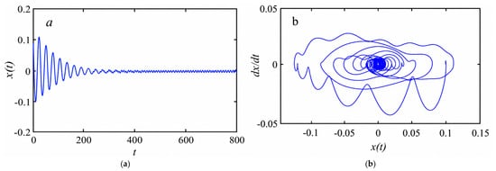
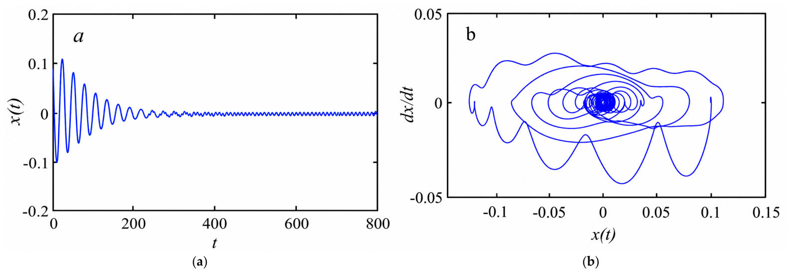
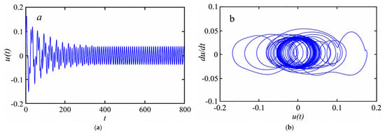
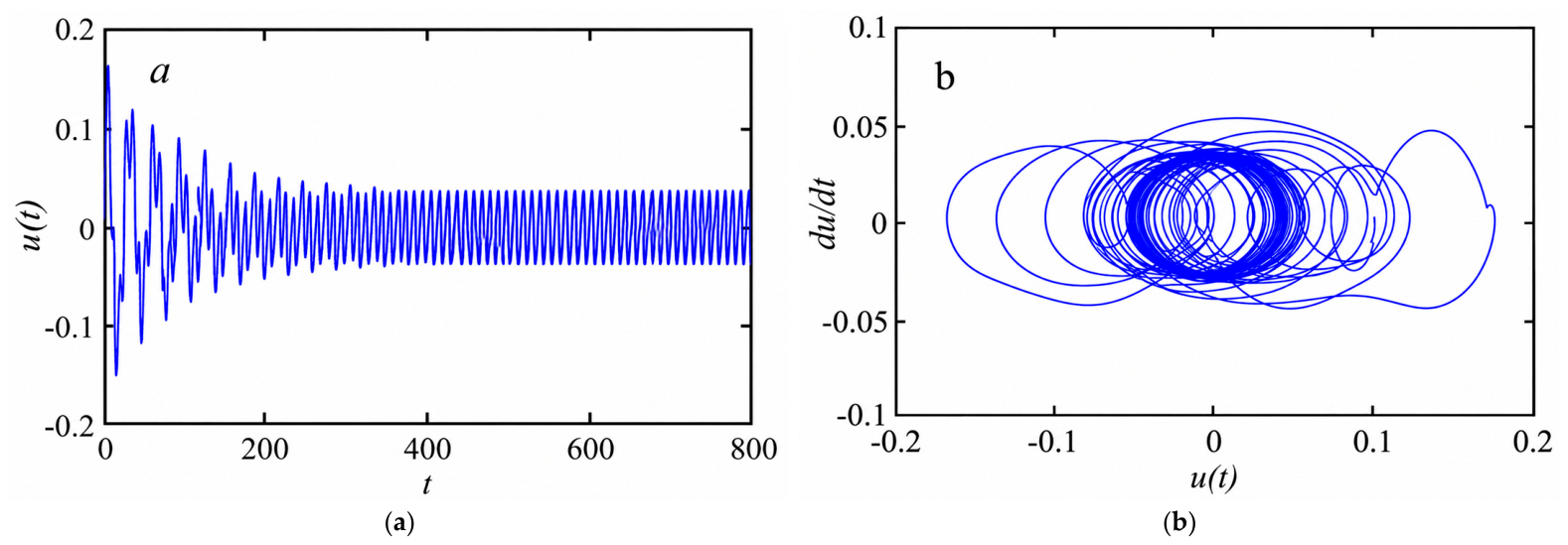
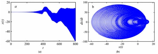
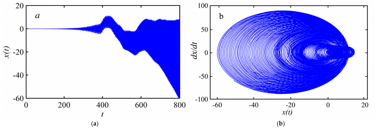
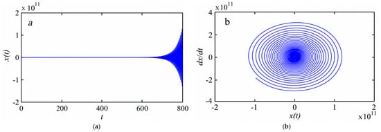
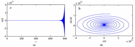
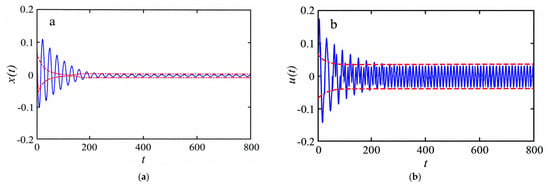
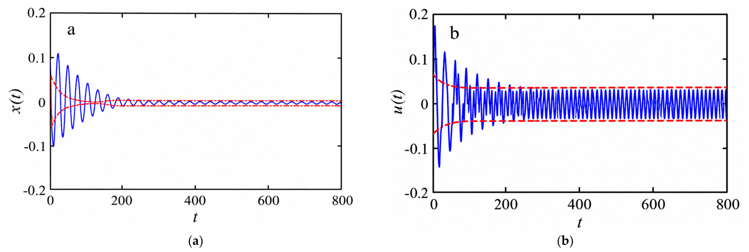
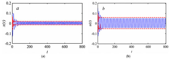
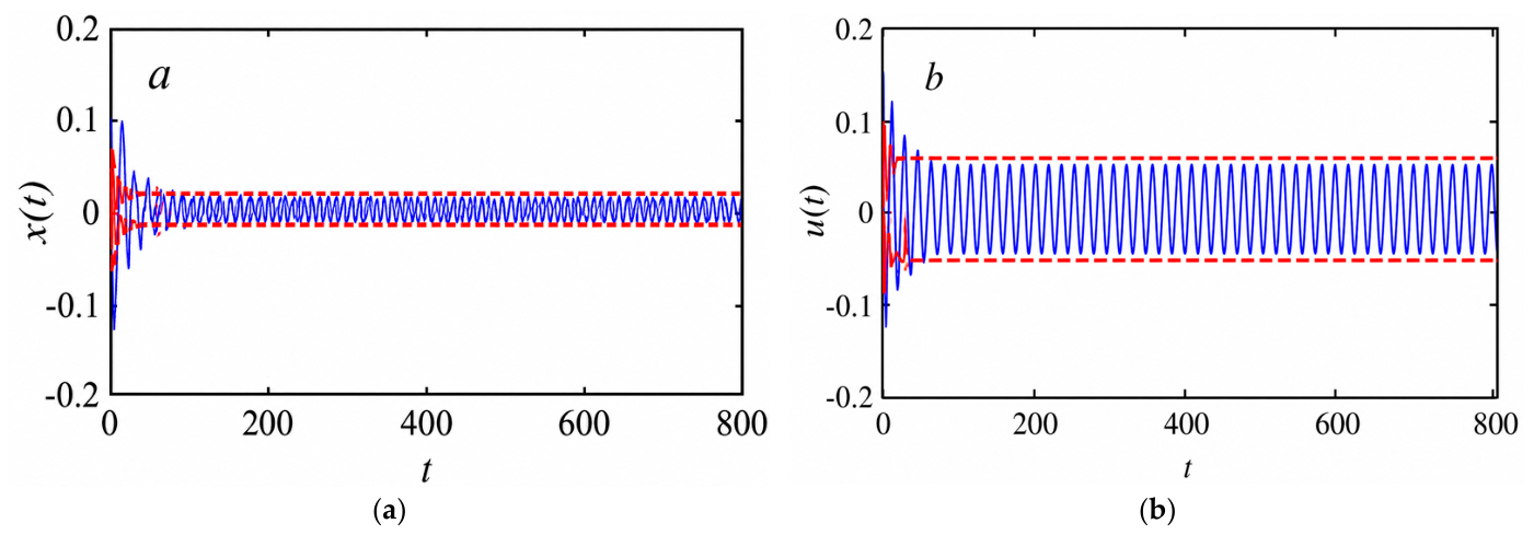
The delayed NDF controller was applied to suppress the vibrations of the main system. Figure 4a illustrates the response amplitude of the controlled system, where the oscillation amplitude decreases to approximately 0.01. This result demonstrates the effectiveness of the delayed NDF controller, with a control efficiency of approximately E_a = 200, where E_a is defined as the ratio of the amplitude without control to the amplitude with control. Furthermore, the phase trajectory converges toward a stable equilibrium point, confirming the capability of the controller to stabilize the system effectively, as illustrated in Figure 4b. Figure 5, Figure 6, Figure 7 and Figure 8 illustrate the time-history responses and phase-plane trajectories of the NDF-controlled system under simultaneous resonance conditions (Ω≈ω₁≈ω₂) for different values of the time delay parameters. Figure 5 demonstrates that the NDF controller operates in a stable periodic regime, where the controller response remains bounded and effectively absorbs vibration energy from the primary system. For (τ₁ = τ₂ = 0.025), we have Figure 6; initially, the system shows small bounded oscillations, and after some time interval, the response amplitude increases progressively, showing the onset of instability due to the time delay. The oscillation amplitude reaches quite large negative values, which shows that the controller is no longer capable of stable vibration suppression. The phase portrait for the corresponding case shows a wide spiral-like trajectory with expanding loops, rather than a compact closed orbit, confirming the presence of the unstable nonlinear behavior and large energy growth in the system. The results show that a moderate delay value can destabilize the controlled response and reduce the effectiveness of the delayed NDF controller in the vicinity of the simultaneous resonance region. However, in Figure 7, when the delay is increased to (τ₁ = τ₂ = 0.03), the system response is unstable, and the oscillation amplitude grows dramatically to the order of 10¹¹, with phase trajectory expanding and not converging to a bounded orbit. Further increase in the delay to (τ₁ = τ₂ = 0.04) in Figure 8 leads to a catastrophic instability, with the amplitude of the response reaching 10³¹, which is a complete loss of stability. The corresponding phase portrait becomes highly divergent, confirming that excessive delay destabilizes the feedback mechanism and causes the controller to inject energy into the system rather than dissipating it. Figure 9 and Figure 10 show a comparison between the numerical results obtained with the Runge–Kutta method and the analytical solutions obtained with the averaging method for the main system and the NDF controller for different sets of parameters. The close agreement between the numerical and analytical responses validates the accuracy and reliability of the averaging analysis. The comparison confirms that the averaging method successfully captures the essential nonlinear dynamics of the controlled system under simultaneous resonance conditions.

(β = 0.2, f = 0.08, τ₁ = τ₂ = 0.005, γ₁ = γ₂ = 3, ζ = 0.3)

(β = 0.1, f = 0.1, τ₁ = τ₂ = 0.007, γ₁ = γ₂ = 2, ζ = 0.6)

Figure 4. (a) The time history and (b) phase of the main system after using a time-delayed NDF controller for the simultaneous resonance case (Ω ≈ ω₁ ≈ ω₂).

Figure 5. (a) The time history and (b) phase plane of the NDF controller for the simultaneous resonance case (Ω ≈ ω₁ ≈ ω₂).

Figure 6. (a) The time history and (b) phase plane of the main system after using the time-delayed NDF controller for the simultaneous resonance case (Ω ≈ ω₁ ≈ ω₂), for (τ₁ = τ₂ = 0.025).

Figure 7. (a) The time history and (b) phase plane of the main system after using the time-delayed NDF controller for the simultaneous resonance case (Ω ≈ ω₁ ≈ ω₂), for (τ₁ = τ₂ = 0.03).

Figure 8. (a) The time history and (b) phase plane of the main system after using the time-delayed NDF controller for the simultaneous resonance case (Ω ≈ ω₁ ≈ ω₂), for (τ₁ = τ₂ = 0.04).

Figure 9. Comparison between the numerical solution (ــــــــــــ) and the averaging analysis (--------) for (a) the main system and (b) the NDF controller with parameters values.

Figure 10. Comparison between the numerical solution (ــــــــــــ) and the averaging analysis (--------) for (a) the main system and (b) the NDF controller with parameters values.

Curves of Averaging Analysis

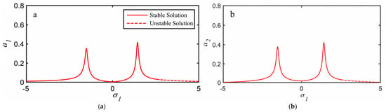
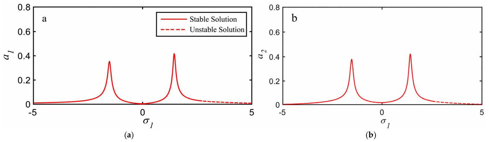
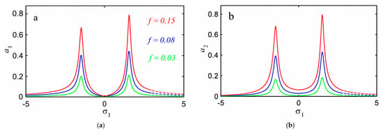
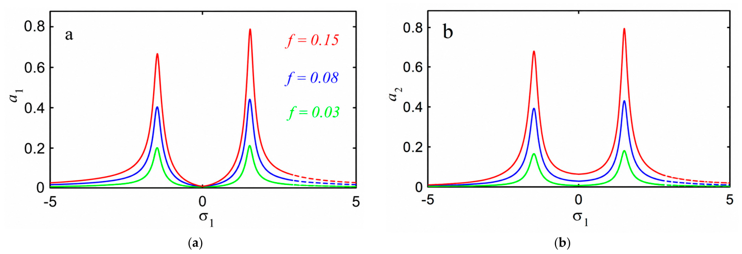
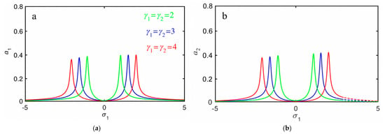
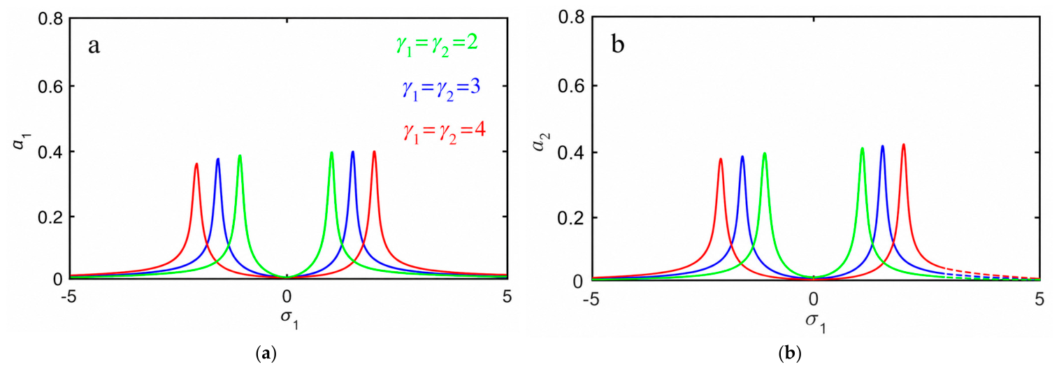
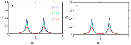
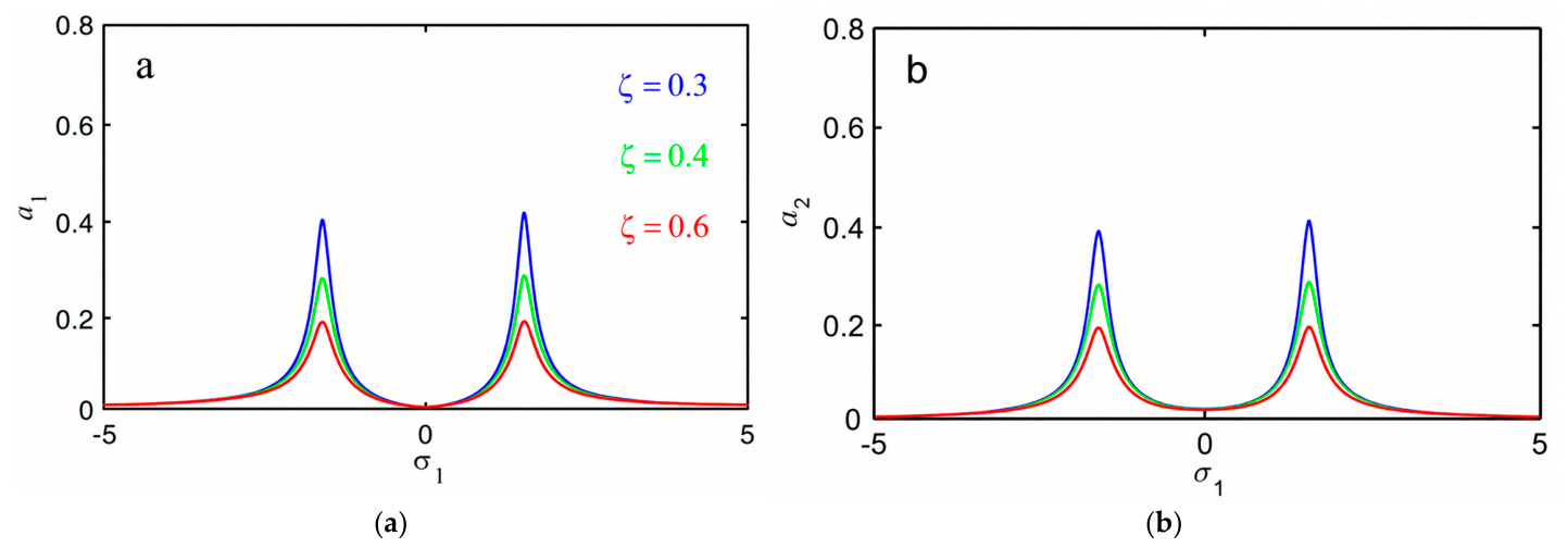
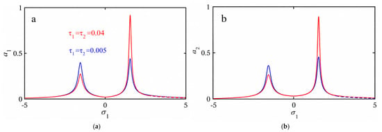
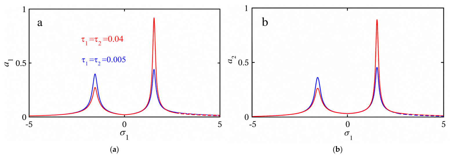
The steady-state amplitudes of the rotating pendulum and the corresponding delayed NDF controller under resonance conditions are determined from the response equations (Equations (45) and (48)). Figure 11 presents the frequency-response characteristics of the primary system and the controller. Two distinct resonance peaks are observed, reflecting the nonlinear interaction between the coupled modes. Both responses contain stable (solid) and unstable (dashed) solution branches. The coexistence of these branches over particular detuning intervals produces multivalued response regions, which are responsible for the associated jump and hysteresis phenomena. Near the tuning condition (σ₁ = 0), corresponding to the minimum vibration level, the response amplitudes decrease considerably. This reduction demonstrates the effectiveness of the delayed NDF controller in suppressing resonant oscillations and improving the dynamic stability of the rotating pendulum. Figure 12, Figure 13, Figure 14 and Figure 15 further clarify how the system and controller parameters modify the resonance zones and the extent of the multivalued regions. Figure 12 illustrates the influence of the external excitation amplitude f. Increasing the excitation amplitude f from 0.03 to 0.15 significantly increases the resonance peaks and strengthens the nonlinear response. Consequently, the multivalued resonance regions become more pronounced, and the unstable branches extend over wider detuning intervals, increasing the possibility of jump and hysteresis phenomena. The controller amplitude also increases with the excitation level, indicating the greater control effort required to suppress the enhanced vibration. Figure 13 demonstrates the influence of the control and feedback gains γ₁ and γ₂. Increasing the gains considerably reduces the amplitudes of the primary system and modifies the locations and widths of the resonance zones. More importantly, the unstable branches and the associated multivalued regions are reduced, indicating that stronger feedback limits the range over which competing steady-state solutions coexist. This behavior can be attributed to the enhanced dynamic coupling and energy transfer from the primary system to the auxiliary controller, resulting in improved vibration suppression. Figure 14 shows the effect of the controller damping coefficient ζ. Increasing the damping decreases the resonance amplitudes and reduces the extent of the unstable branches and multivalued regions. At the same time, the separation between the two resonance peaks increases. Physically, higher controller damping enhances energy dissipation and weakens the nonlinear resonance amplification, thereby reducing the susceptibility of the system to jumps between coexisting response branches. The corresponding reduction in the controller amplitude further confirms the improvement in the overall dynamic stability. Finally, Figure 15 illustrates the influence of the dual time-delay parameters. Unlike the control gain and damping, the delays primarily modify the phase relationship between the measured response and the feedback action. For small delays, the feedback remains favorably phased, and moderate resonance amplitudes are obtained. Increasing the delays shifts the resonance peaks and changes the stable–unstable transition points, thereby modifying the width and location of the multivalued regions. At larger delays, the phase shift introduced into the feedback can reduce the effective damping action of the controller, resulting in enlarged unstable regions and deterioration of the vibration-suppression performance. Therefore, the dual delays cannot be regarded merely as implementation parameters; together with the feedback gains and controller damping, they constitute important tuning parameters governing the resonance location, multi-stability, and stability boundaries of the coupled nonlinear system.

Figure 11. The frequency response curves of (a) the main system and (b) the NDF controller.

Figure 12. The external force action on the frequency response curves of (a) the main system and (b) the NDF controller.

Figure 13. The control and feedback signals’ action on the frequency response curves of (a) the main system and (b) the NDF controller.

Figure 14. The controller damping coefficient’s action on the frequency response curves of (a) the main system and (b) the NDF controller.

Figure 15. The time-delay action on the frequency response curves of (a) the main system and (b) the NDF controller.

5. Comparison with Previous Work

Alluhydan and Abd El-Salam [18] investigated the vibration suppression of a nonlinear rotating pendulum by using a negative delayed acceleration feedback with an effectiveness of about E_a ≈ 3. Compared with the previous work, a bidirectional coupled second-order NDF controller with two feedback gains and two independent time delays is proposed in the present study. Qualitatively, the proposed controller offers an extra method of vibration energy transfer and dissipation via the auxiliary damped system, resulting in smaller resonance amplitudes and unstable response regions for appropriate parameter values. The double delays also allow for more flexibility in tuning. However, too much delay can move the resonance zones and enlarge the unstable regions due to unfavorable feedback phase shifts. Therefore, coordinated tuning of the controller gains, damping and delays is crucial for effective vibration suppression and stability. Also, the effect is about E_a ≈ 200.

6. Conclusions

Based on the analytical and numerical investigations of the vibration control of a nonlinear rotating pendulum using a time-delayed negative derivative feedback (NDF) controller under simultaneous resonance conditions, the following conclusions can be drawn:

• Controller Effectiveness
  The proposed time-delayed NDF controller provides significant vibration suppression in the nonlinear rotating pendulum. The control efficiency is defined as the ratio between the amplitudes without and with control and is about E_a ≈ 200, which means a significant reduction in the vibration amplitude. The corresponding phase trajectories tend toward stable equilibrium states, which verifies the stabilizing capability of the proposed control strategy.
• Analytical and Numerical Validation
  The averaging method gives good approximate analytic solutions to the controlled nonlinear system. Analytical predictions and fourth-order Runge–Kutta simulations are in excellent agreement, thus validating the applicability of the analytical approach for describing the essential nonlinear dynamics under simultaneous resonance.
• Influence of Control and Feedback Gains
  In general, vibration suppression improves, and the length of unstable solution branches decreases. Increasing the control gain γ₁ and feedback gain γ₂ generally helps. The higher the gain value, the lower the response amplitude and the better the system’s stability. This means that more energy is dissipated via the feedback mechanism.
• Role of Controller Damping
  The increase in the controller damping coefficient ζ is reducing the resonance peak and unstable areas. At the same time the resonance bandwidth becomes wider. Hence, damping of the controller is important to balance the vibration attenuation, energy dissipation and overall stability characteristics of the controlled system
• Critical Effect of Time Delays
  The time delay (the time variable and the time-delay parameter τ are dimensionless quantities) is a critical factor in the stability of the controlled system. Small delays, such as τ₁ = τ₂ = 0.01, give stable responses with moderate amplitudes. Reducing the delays to ~(0.025) increases the oscillations progressively and leads to instability. For τ₁ = τ₂ = 0.03, a severe instability is found with amplitudes of the order of 10¹¹, while delays of (0.04) lead to extreme instability with amplitudes of the order of 10³¹. The results show that large delays in feedback can turn the intended dissipative action of the controller into an amplifier and cause severe dynamic instability.
• Nonlinear Frequency-Response Characteristics
  The frequency-response curves exhibit typical nonlinear characteristics such as multiple solution branches, resonance peaks and jump phenomena. The minimum response amplitude occurs close to the tuning condition σ = 0, indicating the effectiveness of the proposed NDF controller, especially close to the fundamental resonance condition.
• Parametric Sensitivity
  The controlled system is very sensitive to the excitation amplitude f, control gains, controller damping and time-delay parameters. With the increase in the excitation amplitude, the resonance peak increases and the resonance region broadens. Proper combinations of the control parameters can significantly improve the vibration suppression and the stability of the system.

Overall, the results demonstrate that the proposed time-delayed NDF strategy can effectively suppress nonlinear vibrations and enhance the stability of the rotating pendulum under simultaneous resonance. However, the strong sensitivity to time delay emphasizes the necessity of carefully selecting the delay parameters to achieve effective vibration suppression without inducing delay-related instability.

References

- Crawford, B.H. Some observations on the rotating pendulum. Nature 1938, 141, 792–793. [Google Scholar] [CrossRef] [Scilit]
- Khan, N.A.; Khan, N.A.; Riaz, F. Dynamic analysis of rotating pendulum by Hamiltonian approach. Chin. J. Math. 2013, 2013, 237370. [Google Scholar] [CrossRef] [Scilit]
- Ciani, G.; Chilton, A.; Apple, S.; Olatunde, T.; Aitken, M.; Mueller, G.; Conklin, J.W. A new torsion pendulum for gravitational reference sensor technology development. Rev. Sci. Instrum. 2017, 88, 064502. [Google Scholar] [CrossRef] [Scilit] [PubMed]
- Rodellar, J. Active control: Concepts and strategies. In Passive and Active Structural Vibration Control in Civil Engineering; Springer: Vienna, Austria, 1994; pp. 275–318. [Google Scholar] [CrossRef] [Scilit]
- Balas, M.J. Active control of flexible systems. J. Optim. Theory Appl. 1978, 25, 415–436. [Google Scholar] [CrossRef] [Scilit]
- Zheng, J.; Krasavin, A.V.; Yang, R.; Wang, Z.; Feng, Y.; Tang, L.; Li, L.; Guo, X.; Dai, D.; Zayats, A.V.; et al. Active control of excitonic strong coupling and electroluminescence in electrically driven plasmonic nanocavities. Sci. Adv. 2025, 11, eadt9808. [Google Scholar] [CrossRef] [Scilit] [PubMed]
- Jamshidi, R.; Collette, C. Optimal Negative Derivative Feedback Controller Design for Collocated Systems Based on H2 and H∞ Method. Mech. Syst. Signal Process. 2022, 181, 109497. [Google Scholar] [CrossRef] [Scilit]
- Amer, Y.A.; Abdullah, R.E.; Khaled, O.M.; Mahdy, A.M.S.; El-Salam, M.N.A. Vibration Control of Smooth and Discontinuous Oscillator via Negative Derivative Feedback. J. Vib. Eng. Technol. 2024, 12, 2351–2363. [Google Scholar] [CrossRef] [Scilit]
- Bauomy, H.S.; EL-Sayed, A.T.; Amer, T.S.; Abohamer, M.K. Negative Derivative Feedback Control and Bifurcation in a Two-Degree-of-Freedom Coupled Dynamical System. Chaos Solitons Fractals 2025, 193, 116138. [Google Scholar] [CrossRef] [Scilit]
- El-Sayed, A.T.; Hussein, R.K.; Amer, Y.A.; Mohammed, F.S.; Alrub, S.A.; Bahnasy, T.A. NDF Controller-Based Stability Analysis and Vibration Mitigation of a Nonlinear Electromechanical Oscillator Under Primary Resonance. Machines 2026, 14, 717. [Google Scholar] [CrossRef] [Scilit]
- Saeed, N.A.; Awrejcewicz, J.; Alkashif, M.A.; Mohamed, M.S. 2D and 3D Visualization for the Static Bifurcations and Nonlinear Oscillations of a Self-Excited System with Time-Delayed Controller. Symmetry 2022, 14, 621. [Google Scholar] [CrossRef] [Scilit]
- Wu, K.; Ren, C.; Chen, Y. Time-Delay Vibration Reduction Control of 3-DOF Vehicle Model with Vehicle Seat. Appl. Sci. 2021, 11, 9426. [Google Scholar] [CrossRef] [Scilit]
- Sinou, J.-J.; Chomette, B. Active Vibration Control and Stability Analysis of a Time-Delay System Subjected to Friction-Induced Vibration. J. Sound Vib. 2021, 500, 116013. [Google Scholar] [CrossRef] [Scilit]
- Sun, X.; Qu, Y.; Wang, F.; Xu, J. Effects of Time-Delayed Vibration Absorber on Bandwidth of Beam for Low Broadband Vibration Suppression. Appl. Math. Mech. 2023, 44, 1629–1650. [Google Scholar] [CrossRef] [Scilit]
- Guo, Y.; Xu, G.-F.; Duan, C.-Y. Research on Time-Delayed Vibration Reduction Control of 1/4 Vehicle Semi-Active Suspension System with Three Degrees of Freedom. Adv. Mech. Eng. 2024, 16. [Google Scholar] [CrossRef] [Scilit]
- Chu, W.; Li, C.; Lyu, Z. Vibration mitigation of flexible beams through boundary motion with enhanced time-delayed control. Thin-Walled Struct. 2025, 210, 113056. [Google Scholar] [CrossRef] [Scilit]
- Amer, Y.A.; El-Sayed, A.T.; Abd El-Salam, M.N. Position and Velocity Time Delay for Suppression Vibrations of a Hybrid Rayleigh-Van Der Pol-Duffing Oscillator. Sound Vib. 2020, 54, 149–161. [Google Scholar] [CrossRef] [Scilit]
- Alluhydan, K.; Abd El-Salam, M.N. Vibration Suppression and Hopf Bifurcation Control in a Nonlinear Rotating Pendulum Using Time-Delayed Acceleration Feedback. AIMS Math. 2026, 11, 21654–21673. [Google Scholar] [CrossRef] [Scilit]
- Nayfeh, A.H. Perturbation Methods; John Wiley & Sons: New York, NY, USA, 2000. [Google Scholar] [CrossRef] [Scilit]
Disclaimer/Publisher’s Note: The statements, opinions and data contained in all publications are solely those of the individual author(s) and contributor(s) and not of MDPI and/or the editor(s). MDPI and/or the editor(s) disclaim responsibility for any injury to people or property resulting from any ideas, methods, instructions or products referred to in the content. |
© 2026 by the authors. Licensee MDPI, Basel, Switzerland. This article is an open access article distributed under the terms and conditions of the Creative Commons Attribution (CC BY) license.