


Abstract
End–edge–cloud collaboration enables significant improvements in system resource utilization by integrating heterogeneous resources while ensuring application-level quality of service (QoS). However, achieving efficient collaborative decision-making in such architectures poses critical challenges within dynamic and complex computing network environments, including dynamic resource allocation, incentive alignment between cloud and edge entities, and multi-objective optimization. To address these issues, this paper proposes a dynamic resource optimization framework for complex cloud–edge collaborative networks, decomposing the problem into two hierarchical decision schemes: cloud-level coordination and edge-side coordination, thereby achieving adaptive resource orchestration across the End–edge–cloud continuum. Furthermore, leveraging differential game theory, we model the dynamic resource allocation and cooperation incentives between cloud and edge nodes, and derive a feedback Nash equilibrium to maximize the overall system utility, effectively resolving the inherent conflicts of interest in cloud–edge collaboration. Additionally, we formulate a joint optimization model for energy consumption and latency, and propose an Improved Discrete Artificial Hummingbird Algorithm (IDAHA) to achieve an optimal trade-off between these competing objectives, addressing the challenge of multi-objective coordination from the user perspective. Extensive simulation results demonstrate that the proposed methods exhibit superior performance in multi-objective optimization, incentive alignment, and dynamic resource decision-making, significantly enhancing the adaptability and collaborative efficiency of complex cloud–edge networks.
Keywords:
complex computing networks; decision-making; network optimization; differential game theory; improved discrete artificial hummingbird algorithm MSC:
94-10
1. Introduction
With the rapid advancement of delay-sensitive applications such as intelligent Internet of Things, augmented reality, and autonomous driving, traditional cloud computing faces increasing challenges in meeting diverse quality-of-service (QoS) requirements due to high latency and bandwidth pressure [1,2]. To address these limitations, end–edge–cloud collaborative computing has emerged as a promising paradigm [3,4], enabling proximity-based task offloading to edge nodes and facilitating hierarchical coordination among terminal, edge, and cloud resources, thereby significantly improving response latency and resource utilization.
End–edge–cloud collaborative networks exhibit inherent complexity, characterized by tier-wise heterogeneity and uneven distribution of resources, as well as significant spatiotemporal dynamics in task workloads [5,6,7]. The interaction of these factors often leads to suboptimal resource efficiency and high latency variability, posing critical challenges for guaranteeing low-latency service delivery [8,9,10]. To address these challenges, existing research has explored diverse resource coordination strategies such as computation offloading and energy management to enhance the efficiency of collaborative computing in distributed edge environments.
Regarding cloud–edge coordination, ref. [11] proposed a digital twin-based resource scheduling model for cloud–edge collaboration, where virtual-real fusion was leveraged to enable adaptive management in dynamic transportation systems. In [12], the authors introduced an intelligent joint channel selection and power control algorithm for heterogeneous networks, which achieved distributed interference management with significantly reduced computational complexity. Ref. [13] developed a layer-aware container update framework that exploited image layering and edge cooperation to minimize download and migration overhead. Ref. [14] presented a multi-agent reinforcement learning approach for vehicular artificial intelligence of things, where application placement and computation allocation were jointly optimized in clustered edge environments. However, the reinforcement learning model suffers from slow convergence and poor adaptability to abrupt changes in network topology, limiting its practical application in dynamic scenarios.
In terms of edge collaboration, the authors in [15] proposed a task scheduling method integrating horizontal edge collaboration and fine-grained partial offloading to minimize completion time through joint optimization of offloading, user–server association, and resource allocation in multi-user edge environments. Ref. [16] introduced a blockchain-based collaboration framework for the Internet of Things, where a Lyapunov-driven hybrid algorithm maximized long-term system utility under security and queue stability constraints. The authors in [17] developed a joint optimization scheme for digital twin-assisted vehicular edge computing, leveraging a TD3-based reinforcement learning algorithm to reduce latency and energy consumption under resource fluctuations. Ref. [18] presented a digital twin-enabled collaboration approach for autonomous vehicles, formulating a coalition-Stackelberg game to optimize service composition and resource pricing for composite services. Although existing research on edge collaboration has made progress in specific scenarios such as horizontal scheduling and digital twin fusion, there is generally a lack of edge–end cross-layer coupling mechanisms, insufficient flexibility in multi-objective optimization, and insufficient balance of interests and demands between edges and terminals, as well as adaptation to terminal resource constraints. In this regard, this paper constructs an edge–end collaborative model, deploys the IDAHA on edge nodes to achieve multi-objective flexible trade-offs, and connects the cloud–edge model through cross-layer coupling mechanisms, effectively addressing the shortcomings of existing research.
For the end–edge–cloud collaboration, the authors in [11] proposed an enhanced proximal policy optimization method for cloud–edge–end collaborative video surveillance in railways, incorporating behavioral cloning and meta-learning to stabilize training and reduce latency under dynamic channel conditions. Ref. [12] designed a multilayer deep reinforcement learning framework for vehicular networks, enabling hierarchical decision-making in task offloading and resource management across vehicle-to-infrastructure and vehicle-to-vehicle links. Ref. [13] developed a recurrent neural network-driven scheduling approach that transformed online task workloads into offline patterns, enhanced by a structured particle swarm optimizer for efficient End–edge–cloud resource allocation. In [19], the authors proposed a hierarchical scheduling approach for multi-tier computing environments, integrating a resource perception model, a long short-term memory-based task decomposition method, and a parallelized deep reinforcement learning algorithm to jointly optimize task execution delay and system energy efficiency. Although existing research on end-to-end cloud collaboration has achieved partial optimization in specific scenarios through reinforcement learning, neural networks, and other methods, there are generally problems, such as complex models leading to high computational costs, insufficient cross-layer dynamic coupling, and ineffective balancing of the interests and demands of multiple entities in cloud–edge end-to-end. This paper adopts a fusion framework of “differential game + improved discrete artificial hummingbird algorithm (IDAHA)” to achieve multi-layer collaborative linkage through cross-layer shared variables and coupling constraints. IDAHA is deployed on edge nodes to adapt to resource constraints, efficiently balancing multi-objective optimization requirements and filling the gaps in existing research.
Beyond the aforementioned shortcomings in end–edge–cloud collaborative research—such as complex models leading to high computational costs, insufficient cross-layer dynamic coupling, and ineffective balancing of multi-entity interests—most existing approaches also rely heavily on static environmental assumptions. This makes them unable to accommodate the persistent dynamics caused by sporadic task arrivals and fluctuating network conditions, resulting in poor adaptability in complex, time-varying real-world scenarios [20]. Moreover, cloud, edge, and end devices operate as autonomous entities with misaligned objectives, and this inherent divergence naturally gives rise to conflicting interests that hinder effective system-wide coordination [21]. In terms of service quality assurance, the majority of current studies adopt single-objective optimization or rigid multi-constraint frameworks, which fail to achieve flexible and adaptive trade-offs between task latency and energy consumption [19,22,23,24]. Furthermore, the intrinsic complexity of multi-objective co-optimization increases the likelihood of converging to suboptimal solutions under dynamic and resource-constrained environments, thereby undermining the practicality and overall performance of scheduling strategies [25].
To address these limitations, this paper proposes a resource coordination optimization framework tailored for dynamic environments. First, a differential game-theoretic approach is employed to model cloud–edge resource allocation and incentive design, where a feedback Nash equilibrium is derived to harmonize conflicting objectives. Second, a joint energy-latency optimization model is formulated, and an enhanced discrete artificial hummingbird algorithm is developed to efficiently search for high-quality solutions, achieving effective dynamic balance among competing objectives.
2. Network Architecture and Collaboration Paradigm
The growing prevalence of latency-sensitive and highly dynamic applications has revealed fundamental limitations in traditional cloud computing, particularly concerning end-to-end latency and excessive bandwidth consumption [26,27]. To overcome these challenges, edge computing decentralizes computational resources by positioning them in proximity to data sources, thereby significantly reducing network congestion and service response times. This architectural evolution has given rise to cloud–edge collaborative computing. As a hierarchical paradigm, it enables intelligent task offloading through real-time assessment of device capabilities, network conditions, and application requirements, thereby achieving an optimal trade-off between energy efficiency and latency performance.
2.1. Network Architecture
As illustrated in Figure 1, the system is divided into centralized cloud infrastructure, distributed edge nodes, and heterogeneous terminal devices, which can, respectively, form an edge-to-edge collaborative architecture and a cloud-to-edge collaborative architecture. Among them, the edge-to-end collaborative architecture connects distributed edge nodes and heterogeneous terminal devices, and undertakes the collection of multi-source data. The tasks generated at the terminal layer can be dynamically unloaded to adjacent edge nodes based on this architecture to achieve low-latency local execution. The cloud–edge collaboration architecture connects the centralized cloud infrastructure with the distributed edge nodes, which are responsible for routing the resource-intensive tasks at the edge nodes to the cloud and relying on the massive computing power of the cloud to complete large-scale analysis.
Figure 1.
Cloud–edge network architecture.
The cloud computing center possesses abundant computational resources and high processing capacity, enabling large-scale data processing and facilitating resource coordination with distributed edge server clusters. The integration of the cloud and edge layers establishes a cloud–edge collaborative computing architecture that supports dynamic computation offloading from edge nodes to cloud servers, thereby enabling cross-tier resource sharing and coordinated task execution. However, due to the significant computation overhead and transmission latency associated with both the cloud center and individual edge nodes, an efficient task offloading and resource allocation strategy is essential to maximize resource utilization and ensure optimal system performance.
Edge server clusters offer significant but finite computational resources, making them well-suited for handling workloads with moderate processing demands. In the cloud–edge collaborative computing architecture, these clusters are paired with groups of end users, enabling the offloading of computational tasks to geographically proximate edge nodes. This proximity supports low-latency execution and enhances service responsiveness. Importantly, many user-side devices are equipped with embedded computing capabilities, allowing them to execute lightweight tasks locally without relying on edge resources. By minimizing redundant data transmission and reducing contention for shared edge capacity, local processing improves overall system efficiency. Consequently, developing intelligent and adaptive resource allocation strategies at the edge layer is essential for optimizing performance, enhancing scalability, and maximizing network capacity in heterogeneous computing environments.
2.2. Cloud–Edge Collaboration Paradigm
The end–edge–cloud collaboration system consists of three core parts: cloud, edge layer, and terminal layer. The component composition, functional positioning, and hardware deployment scheme of each layer are shown in Figure 2. As shown in Figure 2, the global resource scheduling center and database server are deployed in the cloud, connected to the edge cluster through the backbone network. The core function is to integrate the resource status of the entire network and output global resource allocation strategies. The edge layer consists of multiple edge nodes, each equipped with a local computing unit, cache module, and communication interface. It is a key hub connecting the cloud and terminals, capable of undertaking cloud policies and directly responding to terminal task requirements. The terminal layer covers heterogeneous terminals such as IoT devices and in-vehicle terminals. Due to limitations in computing power and energy consumption, it only performs lightweight tasks such as data collection and simple preprocessing. The hardware characteristics and functional division of each layer component provide a physical foundation for the subsequent hierarchical framework of “cloud edge differential game + edge end IDAHA optimization”.
Figure 2.
Cloud–edge collaborative work model.
2.3. Edge–End Collaboration Paradigm
On this basis, the interaction logic and decision transmission path of each layer are shown in Figure 3. From Figure 3, it can be clearly seen that the collaborative process is divided into three key steps: (1) the terminal layer uploads local state information to the edge nodes through the uplink; (2) after summarizing the terminal status, the edge nodes provide feedback on global resource requirements to the cloud and run the IDAHA to complete local offloading decisions; and (3) based on the global load status feedback from the edge layer in the cloud, a resource scheduling strategy is generated through a differential game model, and the computing resource allocation scheme is adjusted downstream to the edge nodes. The information flow of “terminal edge cloud” and the strategy transmission mechanism of “cloud edge terminal” achieve dynamic closed-loop collaboration, ensuring real-time processing of local tasks and efficient utilization of global resources. Figure 2 and Figure 3 jointly clarify the physical carrier and logical interaction basis of the system in this study, providing a direct basis for defining state variables in subsequent differential game models and setting decision objectives for the IDAHA.
Figure 3.
Edge–end collaborative work model.
2.4. Method Design
In response to the hierarchical optimization requirements of end–edge cloud collaboration, this study specifically chooses the fusion framework of “differential game + improved discrete artificial hummingbird algorithm (IDAHA)”. The method selection criteria and advantages are as follows:
At the cloud–edge collaboration level, there is a natural conflict of interest between the cloud and edge nodes (the cloud pursues efficient utilization of global resources, while edge nodes focus on low-latency response to local tasks), and the policy interaction between the two exhibits temporal continuity with dynamic changes in task load and network status. Traditional static games, such as Stackelberg games, can only depict decision equilibrium at a single point in time and cannot adapt to strategy iteration in dynamic scenarios; Differential games can capture the interaction process in the time dimension through the continuous evolution of state variables, and their feedback Nash equilibrium can achieve long-term stable collaborative optimization, avoiding system imbalance caused by short-term optima, thus becoming the optimal choice for cloud–edge dynamic collaborative modeling.
At the edge–end collaboration level, the decision to unload terminal tasks is essentially a 0–1 discrete optimization problem, which requires synchronous balancing of multiple objectives such as latency, energy consumption, and transmission bandwidth. In existing discrete optimization methods, BPSO is prone to getting stuck in local optima, and BGA convergence speed is slow, both of which make it difficult to meet the real-time and optimization accuracy requirements of terminal tasks. To this end, this study improves the traditional artificial hummingbird algorithm by introducing a V-shaped transformation function to adapt to discrete decision-making, designing an adaptive mutation strategy to enhance global optimization capabilities, and forming the IDAHA. At the same time, considering the constraint of the limited computing power of terminal devices, IDAHA is deployed on edge nodes with sufficient computing power, which not only solves the problem of algorithm computational complexity but also improves the scientificity of decision-making through the global state perception ability of edge nodes. Compared with other discrete optimization methods, it is more suitable for the core requirements of edge–end collaboration.
Two methods connect cross-layer shared variables (such as real-time load coefficients of edge nodes) with coupling constraints to form a hierarchical collaborative framework of “cloud–edge dynamic game + edge edge discrete optimization”, accurately matching the core characteristics of end-to-end cloud collaboration. Compared with single optimization methods or static modeling schemes, it can more efficiently solve resource collaboration problems in complex scenarios.
2.5. Key Coupling Mechanisms for the Unified Framework
To clarify the organic integration of the two core components and validate the rationality of the “unified framework”, the specific coupling logic and constraint transmission mechanisms are elaborated upon as follows:
Bidirectional coupling constraint: The task offloading ratio Ctr2(t) output by the cloud–edge differential game (ranging from 0 to 1) serves as a hard constraint for the edge–end IDAHA. Specifically, the proportion of tasks that the IDAHA decides to offload to the cloud cannot exceed Ctr2(t), ensuring that the edge node’s offloading behavior does not exceed the computing resource quota allocated by the cloud. Conversely, the global load status feedback from the edge layer is an important input for the cloud’s differential game model, enabling the cloud to dynamically adjust the computing power allocation coefficient Ctr1(t) based on the aggregated edge load, forming a closed-loop collaborative mechanism.
Consistency of optimization objectives: Both the differential game and IDAHA take “maximizing system utility” as the core goal, but with a hierarchical focus. The cloud–edge differential game emphasizes global resource utilization and long-term interest balance, while the edge–end IDAHA focuses on local multi-objective trade-offs (latency and energy consumption). The coupling constraint Ctr2(t) ensures that the local optimization of the edge–end does not deviate from the global optimization direction of the cloud–edge, realizing the unity of local and global objectives.
3. Cloud–Edge Collaboration Model
Modern distributed systems continuously generate large volumes of sensory and operational data, which are streamed into the network and trigger significant computational demands for real-time analytics, model inference, and system coordination. Traditional edge computing architectures often fail to meet these dynamic and resource-intensive requirements due to the limited capacity of edge nodes. To enhance computational scalability and efficiency, a cloud–edge collaborative network model is introduced to enable joint resource utilization across hierarchical layers.
Cloud–edge cooperation is modeled using differential game theory, capturing the strategic interaction between edge and cloud entities as a dynamic non-cooperative game. This formulation allows the system to converge to a feedback Nash equilibrium, where each participant optimally adjusts its task offloading and resource allocation policy in response to the other’s strategy. At equilibrium, a stable and efficient operating point is achieved, balancing workload distribution, minimizing system-wide energy consumption, optimizing resource allocation, and improving overall network performance. The mathematical symbols and physical meanings involved in the system model are shown in Table 1:
Table 1.
Comparison table of computing task client model symbols. P (*) where * represents the input value of the function.
3.1. Formal Definition of Differential Game Theory
To clarify the interaction rules and optimization objectives of each participant in the cloud–edge collaboration process, this study constructs the cloud–edge collaboration problem as a two-person non-zero sum differential game model, with the formal definition of its core elements as follows:
3.1.1. Players
The participants in the game are two independent decision-makers, namely the following: Participant 1 (cloud): Responsible for the allocation and scheduling of global computing resources such as CPU computing power and storage bandwidth, with the goal of maximizing network resource utilization and long-term revenue; and Participant 2 (edge node): Responsible for local task processing and offloading decisions, with the goal of minimizing the average latency and energy consumption of local tasks.
The scenario of multiple edge nodes can be achieved through the extension of the two-player game, where each edge node independently forms a game pair with the cloud without interfering with each other.
3.1.2. State Space
Define the continuous time state vector of the game as State(t), t∈[0,+∞] is a time variable. The physical meanings and value ranges of each dimension are as follows: State(t) = [St1(t), St2(t), St3(t)]T.
St1(t) represents the length of the task queue at time t of the edge node, reflecting the local task load status, with a range of values; St2(t) represents the real-time computing power allocated by the cloud to the edge node; remaining is the energy consumption ratio of St3(t) edge node at time t.
3.1.3. Control Sets
The control variables and control sets for each participant are defined as follows.
The control variable Ctr1(t)∈U1 for cloud participant P1 in the cloud is the computing power allocation adjustment coefficient, which reflects the dynamic computing power allocation strategy of the cloud to edge nodes. The value range U1 = [0, 1], where Ctr1(t) = 0 represents maintaining the current computing power, and Ctr1(t) = 1 represents allocating the maximum adjustable computing power.
The control variable Ctr2(t)∈U2 of edge node Participant P2 is as follows: task offloading ratio, reflecting the proportion of edge nodes offloading local tasks to the cloud, with a value range U2 = [0, 1]. U2 (t) = 0 means all local execution, and U2(t) = 1 means all uninstallation. The control set must satisfy U1, U2∈R, and the control variables must be piecewise continuous functions.
3.1.4. Information Structure
The game adopts a fully information dynamic structure: Participants P1 and P2 can observe the complete values of the state vector State(t) in real time, including the impact of each other’s decisions, and the decisions only rely on the current state State(t), without relying on historical states and decisions. This information structure is in line with the actual scenario of cloud–edge collaboration, where cloud and edge nodes can interact with each other in real-time through the network for status information.
3.1.5. Horizon
The game has an infinite horizon, i.e., t∈[0,+∞). The reason is that end–edge cloud collaboration is a continuous dynamic process, and there is no fixed termination time for task load and network state. An infinite horizon can better characterize the long-term stable collaborative optimization objective, avoiding the “optimal terminal time” and long-term conflicts of interest under finite time.
3.2. Construction of Income Function
In order to simplify the revenue function model and complete the preliminary verification of the model, the system does not consider the data volume, network status, system load, and other factors separately, but uses a unified amount to calibrate the task volume. Assuming that the revenue function of any edge server at time t is J(t), the savings of uploading tasks to the cloud computing resources are defined as Ssave, the cost of uploading tasks to the cloud is Sup, and the cost of completing the calculation on the cloud and returning the results to the edge is Sdown.
According to the above definition, the income function J(t) can be expressed as
The computing resource savings Ssave of uploading tasks to the cloud can be expressed by the difference between the computing resource cost Sc of tasks processed in the cloud and the computing resource cost of tasks processed at the edge:
It can be assumed that the cloud–edge collaborative computing network system conforms to the quadratic cost function, and the computing cost required by the cloud computing center (CCC) and any edge computing node (ECN) is the square of the computing task it undertakes. The energy consumption per unit CPU cycle of processing computing tasks is positively correlated with the square of the computing power of the device.
Based on the above research, the calculation capacity of CCC is defined as fc, and the calculation capacity of ECNi is defined as fe,i, and the energy consumption per CPU cycle of CCC and ECNi is, respectively,
where is a constant, depending on the CPU structure of CCC; is a constant, depending on the CPU structure of ECN.
The energy consumption cost per unit time CPU generated by CCC can be expressed as
The energy consumption cost of ECNi per unit CPU time can be expressed as
The parameters Kc and Ke, respectively, represent the weight coefficients of the task’s consumption cost when calculating in CCC and ECN. The higher the weight value, the lower the energy consumption should be.
The calculation cost of CCC and ECN can be expressed as a quadratic cost function, and the calculation cost of CCC processing at time t can be expressed as
Similarly, the calculation cost of ECN at time t can be expressed as
where u(t) represents the number of tasks uploaded to CCC at time t, and x(t) represents the number of tasks planned to be transferred from the edge to the cloud at time t.
At time t, the calculation cost of the number of tasks uploaded to the cloud Sup is related to the number of tasks currently planned to upload to the cloud x(t). To simplify the model, it can be approximately considered that Sup is linearly related to the size of x(t), which can be expressed as
Among them, λ represents the task allocation cost parameter, meeting λ > 0.
The cost Sdown of the calculation result returned to the edge can be expressed as a quadratic cost function:
where ε refers to the cost parameter when the task calculation result is returned, satisfying ε > 0.
According to the above, the income function J(t) can be expanded as
3.3. Objective Function Construction
According to the differential game theory, the system objective function can be constructed:
The first addend of the objective function represents the cumulative income, the second addend represents the final benefit calculated according to the system state, r represents the discount rate, e−r(t−t0) represents the discount factor, which can reflect the proportion of future income in the current income value. The entire objective function represents the cumulative benefits of the cloud–edge collaboration system at time T.
3.4. Construction of Task Volume Change Function
Assuming that the number of user tasks added at time t is Nuser, the value of Nuser is related to the maximum rate Re of task application submitted by the user at that time and the maximum carrying capacity Ce of edge storage tasks, and the number of new tasks can be expressed as
Assuming that the number of tasks uploaded at the edge at time t is Nout, the value of Nout is related to the upload task rate Ri transmitted from the edge to the cloud and the maximum capacity Ci that can be stored. The number of uploaded tasks of ECNi can be expressed as
According to Shannon’s theorem, we can get
Bi represents the transmission bandwidth, and Si/Ni represents the signal-to-noise ratio.
Then we can express the number of tasks uploaded to the cloud at time t as
3.5. Value Function Construction
The resource allocation of cloud–edge collaborative computing meets the following partial differential equation of the value function:
where t represents time, x represents state, V(t,x) is the value function within the time interval [t0,T], and f represents the rate of change of state x. Formula (16) can be used to represent f.
The value function V(t,x) can be expressed as the integral of the product of the income function J and the discount factor in the time from t0 to T:
3.6. Solve the Task Amount Upload Function
Substitute Formulas (11) and (16) into the first differential equation of Formula (17) to get
At time T, the value of the value function Vi(t,x) can be expressed as follows according to the second equation of Formula (17):
The derivation of Formula (19) with respect to u and its derivative being 0 can be solved as follows:
where M is expressed as
where G is expressed as
Then, it can be assumed that the value function and parameters A (t), B (t) meet the following relationship:
The partial derivative of Formula (24) to t is
If Formula (25) is sorted into the same form as Formula (17), we can get
The partial derivative of Formula (24) to x can be obtained:
Substitute Formula (27) into Formula (21):
Substitute Formulas (11), (27), and (28) into Formula (19) to get
After simplification, we can get
Comparing Formula (26) with Formula (30), we can get
Formula (31) is sorted into the form of a first-order linear ordinary differential equation:
The equation satisfies
Therefore, it can be obtained that
When t = T, A(t) satisfies
Therefore, according to the initial value correspondence, we can get
Substitute Formula (36) into Formula (34) to get
Substitute Formula (37) into Formula (28) to get a feedback Nash equilibrium solution of strategy [u*(t)]:
3.7. Strict Rationality Demonstration of HJB Equation Application
This article applies the HJB equation to solve the infinite time domain two-person non-zero sum differential game of cloud–edge cooperation, and its rationality stems from the following theories and scene adaptability:
The cloud–edge interaction is modeled as a continuous-time dynamic game with fully observable states, which is consistent with the core premise of solving differential games using HJB equations—participants can obtain the system state in real time and dynamically optimize strategies, meeting the compatibility of game structure. As shown in Section 3.2, the system adopts a quadratic cost function (Equations (7) and (8)) and linear state dynamics (Equation (39)). For infinite time domain LQ differential games, the HJB equation is a standard and rigorous tool for deriving a feedback Nash equilibrium, and the quadratic structure ensures the existence of closed-form solutions. The infinite time domain characteristics of the game ensure that the value function V(t, x) converges to a time-invariant solution, avoiding inconsistencies caused by terminal conditions and meeting the requirements of the HJB equation for asymptotic stability of the value function.
The existence and uniqueness of solutions to the HJB equation (Equation (17)) are guaranteed by the following assumptions, which all hold true in our model:
Assumption 1.
(Quadratic value function assumption): We assume V(t, x) = A(t)x2+ B(t)x + C(t) (Equation (24)). For LQ games, due to the linear state dynamics and quadratic cost function, this form is consistent with the structure of the HJB equation and is a reasonable assumption for the solution.
Assumption 2.
(Discounted utility): The discount factor e−r (t−t0) in Equation (12) satisfies r > 0, ensuring that the infinite time domain integral is bounded and avoiding the solution being non-unique due to unbounded utility accumulation.
Under the above assumptions, according to the classical LQ differential game theory, the HJB equation (Equation (17)) has a unique time invariant solution V(x)= Ax2 + Bx + C.
The control u*(t) (Equation (38)) derived in this article fully satisfies the core conditions that each participant’s strategy is optimal under the given strategy of the other party, and the strategy depends only on the current state, as two feedback Nash equilibria. By taking a partial derivative of the HJB equation with respect to u and making it zero (Equation (21)), the optimal response of edge nodes to cloud–edge computing power allocation is obtained, satisfying the “optimal response” condition of Nash equilibrium. Equation (38) only relies on the current state x(t) and time-varying coefficient A(t), and does not involve historical states or decisions, which conforms to feedback characteristics.
3.8. Solve the Task Volume Function
Substitute Formula (38) into Formula (16) to get the task amount change function:
Numerical integration is solved according to the Euler method:
Substitute Formula (39) into Formula (40) to get
The delay term in the objective function is strictly convex, and the linear combination of convex functions remains convex. The constraints are all linear, so this problem belongs to the convex optimization problem. This problem is a continuous variable optimization problem and belongs to a polynomial-time solvable problem. Convexity ensures the existence of a unique global optimal solution to the problem. Combining the “dynamic temporal” characteristics of the problem, this study chooses differential game theory + HJB equation solution—HJB equation can efficiently capture the optimal strategy evolution in continuous time, complementing the unique solution characteristics of convex optimization to ensure the stability and optimality of the computing power allocation strategy.
The pseudocode of the differential game model is shown in Algorithm 1.
| Algorithm 1. Differential Game Model Solving Process for Cloud–Edge Collaboration | |
| Input: Terminal device set: Edge server set: Initial parameters: Task data size Di(t) device computing capacity fi(t) edge computing capacity Fj(t) Weight coefficient: λ Discount rate r Time horizon T Output: Optimal upload strategy u*(t) Task transfer amount x(t) System value function V(t, x) Total system utility J(t) | |
| Initialize: | |
| 1 | Set initial state x(0), control variables Ctr1(0), Ctr2(0) |
| 2 | Initialize value function parameters A(0), B(0), C(0) |
| 3 | Set time step Δt, iteration index k = 0 |
| Procedure: | |
| 4 | while t ≤ T do |
| 5 | 1. Compute revenue function J(t) |
| 6 | J(t) = Ssave − Sup − Sdown |
| 7 | where |
| 8 | Ssave = Sc − Se, Sup =λx(t), Sdown =εu2(t) |
| 9 | 2. Solve HJB equation for optimal control u*(t) |
| 10 | |
| 11 | Derive optimal upload strategy: |
| 12 | |
| 13 | 3. Update task dynamics x(t) using Euler method |
| 14 | |
| 15 | 4. Update value function parameters A(t), B(t) |
| 16 | Solve ODE system: |
| 17 | |
| 18 | 5. Check equilibrium condition |
| 19 | Compute equilibrium index: |
| 20 | |
| 21 | if η(t) ≥ 0.95 then |
| 22 | Output: System reaches feedback Nash equilibrium |
| 23 | break |
| 24 | end if |
| 25 | |
| 26 | end while |
| 27 | Return: |
| 28 | u*(t): Optimal upload strategy |
| 29 | x(t): Task transfer trajectory |
| 30 | V(t, x): System value function |
| 31 | Convergence time teq |
4. Edge–End Collaboration System Model
In the field of edge network, in addition to the business requirements with a large amount of data and computation, there are also some businesses, such as real-time production and optimization, intelligent patrol, and security monitoring. Cloud–edge collaborative network is difficult to meet its low-latency requirements. In order to solve these problems, this research proposes the edge collaboration mode, which schedules the computing resources of the edge server and the user equipment itself for processing, reduces the overall delay and energy consumption of task processing, and achieves the goal of optimizing network efficiency.
The edge network collaboration system is generally composed of the user layer, transport layer, and computing layer. Users accessing the network at the user layer will generate computing tasks and send them to the network nodes at the transport layer. The transport layer will make unloading decisions according to intelligent algorithms, and then allocate computing resources of edge servers and mobile devices according to the unloading decisions, so as to complete the processing of computing tasks at a lower cost.
4.1. Computing Task Client Model Construction
When computing tasks locally, it is mainly considered to build a delay model and an energy-consumption model for tasks to perform local computing on user equipment. Relevant mathematical symbols and their physical meanings are shown in Table 2:
Table 2.
Comparison table of computing task client model symbols.
The system delay when the calculation task is executed locally is shown in Formula (42):
To ensure a good quality of experience (QoE), the delay of computing task execution should meet Formula (43):
The system energy consumption during calculation when the calculation task is executed locally is shown in Formula (44):
where k is a constant, which depends on the architecture of the micro-integrated circuit, and is usually 10−27. represents the energy consumption of each CPU cycle when the local terminal executes computing tasks. Due to the limited computing power of the CPU, the computing power of the local terminal needs to meet the Formula (45):
To sum up, when the user task set is , the user task label is represented by i, and the system delay and system energy consumption weighted value calculated by the system are taken as the system cost Plocal. The mathematical model of computing tasks all executed at the local terminal is shown in Formula (46):
where C1 represents that the delay of local calculation should be within the delay threshold of completing the calculation task; C2 means that the computing capacity of the local terminal is less than the maximum value of the computing capacity of the local terminal; and C3 means that the weighting coefficient should be between 0 and 1.
λ is the global balance coefficient between time delay and energy consumption, used to unify the order of magnitude and units of the two and avoid dimensional differences affecting optimization bias. By adjusting λ, it can adapt to different scene requirements: when λ is too small, it focuses on time delay optimization; when λ is too large, it focuses on energy consumption optimization; when λ is in the middle, it achieves a balance between the two, and the model solution dynamically adjusts with λ rather than being fixed and unique.
4.2. Computing Task Edge Model Construction
When computing tasks need to be offloaded to the edge server for computing, the main consideration is to build a delay model and an energy-consumption model for offloading computing. The system delay is also related to the transmission rate, which is determined by the transmission bandwidth and the receiver’s signal-to-noise ratio. Therefore, it is also necessary to establish the transmission rate model of the impact of the transmission rate on the system. The required mathematical symbols and their physical meanings are shown in Table 3:
Table 3.
Comparison of model symbols at the edge of the calculation task.
When computing tasks are unloaded to the edge server for execution, the transmission rate of the system needs to be considered, which is related to the transmission bandwidth of the channel. The transmission rate model of the system is shown in Formula (47):
To simplify the model, it is advisable to assume that the signal-to-noise ratio at the receiving end of the system is fixed. When the signal-to-noise ratio at the receiving end of the system is fixed, it can be considered that the transmission rate of the system is positively correlated with the transmission bandwidth, and the change in the transmission bandwidth can be represented by the change in the transmission rate, so that the transmission bandwidth can be allocated and optimized by allocating the transmission rate of the system.
The computing power of the edge server is affected by the system transmission rate. The computing power of the edge server is shown in Formula (48):
The system delay when computing tasks are unloaded to the edge server for execution consists of data transmission delay and edge computing delay. The data transmission delay is shown in Formula (49):
The edge calculation delay is shown in Formula (50):
The above two delay models are accumulated to obtain the delay model of computing tasks offloaded to the edge server for execution, as shown in Formula (51):
Similarly, the system energy consumption of computing tasks offloaded to the edge server consists of transmission energy consumption and computing energy consumption. Transmission energy consumption is shown in Formula (52):
The calculated energy consumption is shown in Formula (53):
Accumulate the above two energy-consumption models to get the energy-consumption model of computing tasks unloaded to the edge server for execution, as shown in Formula (54):
To sum up, when computing tasks are unloaded to the edge server for execution, the weighted value of system delay and system energy consumption calculated by the system is taken as the system cost Pedge. The mathematical model of computing tasks all executed on the edge server is shown in Formula (55).
Wherein, C1 represents that the system delay of the calculation task unloaded to the edge server should be within the delay threshold of completing the calculation task; C2 restricts the computing power of the edge server; C3 means that the total computing capacity of all edge servers when performing computing tasks is less than the total computing capacity of the entire computing network server; C4 means that the weighting coefficient should be between 0 and 1.
The physical meaning of λ is consistent with Formula (46), which is a globally unified delay energy balance coefficient. Its core function is to coordinate the optimization weights of two non-dimensional objectives, ensuring that the model can flexibly adjust the optimization bias according to actual application scenarios.
4.3. Computing Task Side Network Collaborative System Model
When processing the system tasks generated by the user layer, the total system delay, the total energy consumption of the system, or the total weighted sum of the energy consumption of the system delay is often considered as the total cost of the system. In order to achieve the lowest total cost of the system when processing computing tasks, it is necessary to allocate the system to decide whether computing tasks are executed locally or unloaded to the edge server, so that computing tasks can be completed with the lowest system cost. The calculation task unloading decision set is shown in Formula (56).
Combined with the local computing and offload computing models described above, the offload decision can be used to combine the local computing and offload computing to build the total delay cost offload model, the total energy consumption cost offload model, and the combined optimization model of delay energy consumption weighting and total cost.
The total delay cost model is shown in Formula (57):
Formula (57) shows that the mathematical model established for the system is the total delay model of the system, and the total delay cost of the system is minimized by optimizing the unloading decision si. Here, C1 means that the unloading decision si should be in the computing task unloading decision set, and the unloading decision values are 0 and 1, si = 0 means that the computing task is executed locally, and si = 1 means that the computing task is unloaded to the edge server for execution; C2 indicates that the total system delay must be within the delay threshold required to complete the task, regardless of whether the calculation task is unloaded or not; C3 means that when the computing task is executed locally, the computing capacity of the local terminal should be within the maximum range of the computing capacity of the local terminal; C4 indicates that when computing tasks are offloaded to the edge server for execution, the edge server meets the computing capacity to complete computing tasks within the delay threshold of edge computing; C5 means that the total computing power of all edge servers should be within the maximum computing power of edge servers.
The total cost model of energy consumption is shown in Formula (58):
Formula (58) shows that the mathematical model established for the system is the weighted sum of the total delay and total energy consumption of the system, and the total cost of the system is minimized by optimizing the unloading decision si. Here, C1 means that the unloading decision si should be in the computing task unloading decision set, and the unloading decision values are 0 and 1. si = 0 means that the computing task is executed locally, and si = 1 means that the computing task is unloaded to the edge server for execution; C2 means that when the computing task is executed locally, the computing capacity of the local terminal should be within the maximum range of the computing capacity of the local terminal; C3 indicates that when computing tasks are unloaded to the edge server for execution, the edge server meets the computing capability of completing computing tasks within the delay threshold of edge computing; and C4 means that the total computing power of all edge servers should be within the maximum computing power of edge servers.
The calculation task joint optimization model is shown in Formula (59):
Formula (59) shows that the mathematical model established for the system is the weighted sum of the total delay and total energy consumption of the system, and the total cost of the system is minimized by optimizing the unloading decision si. Here, C1 means that the unloading decision should be in the computing task unloading decision set, and the unloading decision values are 0 and 1, si = 0 means that the computing task is executed locally, and si = 1 means that the computing task is unloaded to the edge server for execution; C2 indicates that the total system delay must be within the delay threshold required to complete the task, regardless of whether the calculation task is unloaded or not; C3 means that when the computing task is executed locally, the computing capacity of the local terminal should be within the maximum range of the computing capacity of the local terminal; C4 indicates that when computing tasks are offloaded to the edge server for execution, the edge server meets the computing capacity to complete computing tasks within the delay threshold of edge computing; C5 means that the total computing power of all edge servers should be within the maximum computing power of edge servers; and C6 indicates that the weighted coefficients of system delay and system energy consumption should be in the range of 0 to 1.
Here, λ continues the previous definition as a global adjustment coefficient for time delay and energy consumption. Its value can be calibrated according to actual scenario requirements, enabling the model to output both energy delay balance solutions and targeted biased optimal solutions, thereby enhancing the model’s practical adaptability.
The delay and energy consumption terms in the objective function are both linear functions with respect to binary variables. However, due to the fact that the variables are discrete 0–1 type and the constraints contain integer constraints, this problem belongs to integer linear programming and is not convex. The scale of the problem increases exponentially with the number of terminals and edge nodes, belonging to NP hard problems. Traditional exact algorithms are difficult to solve within real-time requirements. The discreteness and NP hard characteristics of this problem are the core reasons why this study chooses the Improved Discrete Artificial Hummingbird Algorithm (IDAHA)—IDAHA can obtain approximate optimal solutions in polynomial time through binary adaptation and global optimization strategies, meeting the real-time requirements of terminal tasks.
4.4. Optimization of Resource Allocation for Edge Collaboration Based on Artificial Hummingbird Algorithm
In the new computing network integration system architecture, in order to ensure efficient computing services for customer servers, it is necessary to ensure the reasonable allocation of system computing resources. For the resource collaborative optimization of computing network, this research abstracts the network nodes in computing network system on the basis of edge computing technology, establishes an objective function with system energy consumption, system delay and transmission bandwidth as the total cost of the system, improves the traditional artificial hummingbird algorithm and uses it to optimize the objective function, so as to realize the resource collaborative optimization of computing network system.
The IDAHA is deployed at the edge nodes with more sufficient computing power and global state aggregation ability to avoid the problem that the terminal node cannot carry out recalculations due to insufficient computing power and suboptimal decision making due to a lack of global vision. On this basis, this study establishes the objective function with the system energy consumption, system delay and transmission bandwidth as the total cost of the system, optimizes the objective function by using the IDAHA, and finally outputs the optimal resource allocation and task unloading decisions and sends them to the corresponding terminal nodes so as to realize the resource collaborative optimization of the computing network system.
The AHA is mainly composed of three parts: food source, hummingbird, and access table. In combination with this study, food source is a solution vector, representing the unloading strategy. The nectar filling rate of each food source corresponds to the value of the objective function, that is, the fitness calculated by the AHA algorithm. The lower the fitness, the higher the nectar filling rate of the food source. The symbols involved in the AHA and their physical meanings are shown in Table 4:
Table 4.
Comparison of AHA symbols and physical meanings.
Hummingbirds are the main part of the algorithm. When the algorithm is initialized, each hummingbird is randomly placed on the food source location, and each hummingbird can remember the visited location and fitness and share them with the whole hummingbird population. Hummingbirds in the population are more inclined to visit new food sources with a high access rate, which have not been visited for a long time.
Population location initialization is shown in Formula (60):
The initialization of the food source location is shown in Formula (61):
The access table records the temporal and spatial information of hummingbirds’ access to food sources, generates the access levels of different hummingbirds to each food source, and avoids hummingbirds’ access to the recently collected food sources. The higher the level of food sources, the priority will be given to hummingbirds.
The AHA algorithm realizes the search for the global optimal solution by simulating three foraging behaviors of hummingbirds, namely, guided foraging, territorial foraging, and migration foraging.
In the process of guided foraging, the new target food source of hummingbirds should have two characteristics: a high nectar filling rate and a long non-visit time. At the same time, hummingbirds will give priority to the food source with the largest number of visits, and when the number of visits is the same, they will give priority to the food source with the highest nectar filling rate. In the process of guided feeding, hummingbirds have three flight behaviors: omnidirectional flight, diagonal flight, and axial flight, so as to better realize the renewal of food sources. The three flight behaviors of hummingbirds guiding foraging are shown in Figure 4:
Figure 4.
Hummingbird guided foraging flight behavior.
Omnidirectional flight is defined as Formula (62):
Diagonal flight is defined by Formula (63):
Axial flight is defined by Formula (64):
In Formula (63), randperm(k) generates a random integer array from 1 to k; r1 is a random number in (0,1); and randi([1,d]) in Formula (64) generates a random integer from 1 to d. According to the above principles, the algorithm realizes various flight foraging modes of hummingbirds, and completes the position update of the i-th food source in the access table.
Guiding foraging and updating food source is defined as Formula (65):
The position update is defined as Formula (66):
In the process of foraging in the territory, hummingbirds may search for other new food sources after collecting nectar from the target food source, search the surrounding space locally according to their location, and move to the adjacent area of their territory. The application table will be updated when the nectar filling rate of the new food source is better than the food source where it is located. At the same time, the new food source will also become the food source that most attracts other hummingbirds in the population. The hummingbird territory foraging diagram is shown in Figure 5:
Figure 5.
Hummingbird territory feeding diagram.
The food source for foraging and updating in the territory is defined as Formula (67):
In the process of migration and foraging, if the number of iterations of the algorithm exceeds the preset migration coefficient, the hummingbird will explore the random food sources randomly allocated to the space again and update the access table.
The migration and foraging position update is defined as Formula (68):
The migration and foraging process is shown in Figure 6:
Figure 6.
Hummingbirds’ foraging process.
In this study, the objective function of the mathematical model of system energy consumption, system delay, and transmission bandwidth is taken as the cost of resource collaborative optimization, and the unloading strategy is taken as the food source solution vector of the hummingbird foraging. Through the various foraging behaviors of hummingbirds, the solution vector tends to the global optimal solution, so as to achieve the collaborative optimal allocation of computing network resources. Since the unloading decision can be regarded as a 0–1 binary problem in this problem, the solution vector of the problem needs to be converted into a binary form to meet the requirements of system optimization.
In order to meet the above requirements, a V-shaped conversion function needs to be defined, which maps the and variables when the hummingbird guides the foraging and updates the food source position to between 0 and 1, and takes the random number r between 0 and 1 as the judgment threshold. The mapped value is compared with the judgment threshold. If it is greater than the judgment threshold, it is considered that the updated food source position is 1, and if it is less than the judgment threshold, it is considered that the updated food source position is 0. The corresponding binary conversion process is shown in Formulas (69) and (70):
Accordingly, the position update Formula (66) for hummingbird guidance foraging is updated to Formula (71):
With reference to the idea of Genetic Algorithm (GA), the adaptive mutation probability is introduced into the AHA. At the initial stage of exploration, there is a large mutation probability, which can better optimize the exploration area. The mutation probability in the later stage of exploration will gradually decrease with the number of iterations, which can provide better convergence for the whole system. The adaptive mutation probability is shown in Formula (72):
In addition, the AHA also introduces the single-point crossover idea of the GA, which allows the hummingbird to exchange some positions with the hummingbird at the target position when guiding the foraging, so as to expand the scope of exploration, improve the exploration ability of the hummingbird, and avoid falling into local optimization. Single point crossing is shown in Formula (73):
The elite guidance strategy, originally proposed to enhance the PSO algorithm, is incorporated into the AHA algorithm in this study. By integrating this strategy, hummingbirds can select food sources based on both the current global optimal solution and the best information stored in the access table. This guidance mechanism enhances the algorithm’s ability to balance exploration and exploitation, thereby improving its overall optimization performance. The implementation of the elite guidance strategy is given in Equation (74):
In the process of guided foraging, hummingbirds have a 50% probability to choose the current global optimal solution for guidance, and a 50% probability to choose the optimal access table for guidance, thus enriching the exploration scope of guided foraging and providing the target location for the single point intersection of Formula (73).
In the process of territorial foraging, this study introduces the strategy of adaptive random multi-bit flipping to increase the diversity of territorial foraging. The probability of flipping will gradually decrease with the number of iterations, thus adapting to the characteristics of the AHA, which is exploratory at the initial stage and has strong convergence at the later stage. Random multi-bit flipping is shown in Formula (75):
In the process of migration and foraging, this study set that if the foraging position of hummingbirds did not change after 20 iterations, 25% of hummingbirds with the worst fitness would be reinitialized.
Based on the above, this study proposes an Improved Discrete Artificial Hummingbird Algorithm (IDAHA) to achieve the optimal allocation of edge collaborative computing resources. By iteratively optimizing the total cost function of the system, the unloading decision with the lowest total cost of the system can be obtained, thus optimizing the edge collaborative computing resources.
The pseudocode of the IDAHA is shown in Algorithm 2.
| Algorithm 2. Improved Discrete Artificial Hummingbird Algorithm (IDAHA) for Edge–End Collaboration | |
| Input: User task set: Task data size: CPU cycles required: Local computing capacity: Edge server computing capacity: fc Weight coefficient: λ Population size: pop Problem dimension: dim = N Maximum iterations: max_iter Output: Optimal offloading decision vector: Minimum system total cost: best_fitness Convergence curve: convergence | |
| Initialize: | |
| 1 | Initialize hummingbird positions (binary): |
| 2 | X = randint(0, 2, (pop, dim)) |
| 3 | Initialize fitness values: |
| 4 | |
| 5 | Initialize visit table: |
| 6 | visit_table = zeros((pop, pop)) |
| 7 | fill_diagonal(visit_table, NaN) |
| 8 | Initialize global best: |
| 9 | best fitness = ∞, best solution = None |
| 10 | Initialize stagnation counter: |
| 11 | stagnation_counter = 0 |
| Procedure: | |
| 12 | for iter = 1 to max_iter do |
| 13 | for i = 1 to pop do |
| 14 | 1. Create direction vector (three flight patterns) |
| 15 | Generate random number r∈[0, 1] |
| 16 | if r < 0.4 then(Diagonal flight (40%)) |
| 17 | rand_num = randint(1, dim − 1) |
| 18 | idxs = random_choice(dim,rand_num,replace = False) |
| 19 | direction[idxs] = 1 |
| 20 | else if r < 0.8 then(Axial flight (40%)) |
| 21 | idx = randint(dim) |
| 22 | direction[idx] = 1 |
| 23 | else(Omnidirectional flight (20%)) |
| 24 | direction = ones(dim) |
| 25 | end if |
| 26 | 2. Guided foraging (70%) or Territorial foraging (30%) |
| 27 | Generate random number r2∈[0, 1] |
| 28 | if r2 < 0.7 then |
| 29 | if rand() < 0.5 then |
| 30 | target_idx = argmin(fitness_vals) |
| 31 | else(Select from visit table) |
| 32 | valid_visits = visit_table[i,¬isnan(visit_table[i])] |
| 33 | if length(valid_visits) > 0 then |
| 34 | min_visit = min(valid_visits) |
| 35 | Candidates = where(visit_table[i] == min_visit) |
| 36 | target_idx = candidate with best fitness |
| 37 | else |
| 38 | target_idx = i |
| 39 | end if |
| 40 | end if |
| 41 | Single-point crossover operation |
| 42 | cross_point = randint(1,dim) |
| 43 | new_pos = X[i].copy() |
| 44 | new_pos[:cross_point] = X[target_idx][:cross_point] |
| 45 | Adaptive mutation |
| 46 | mutation_prob = 0.1 × (1 − iter/max_iter) |
| 47 | for j = 1 to dim do |
| 48 | if rand() < mutation_prob then |
| 49 | new_pos[j] = 1 − new_pos[j] |
| 50 | end if |
| 51 | end for |
| 52 | else |
| 53 | Territorial foraging |
| 54 | new_pos = X[i].copy() |
| 55 | Adaptive random multi-bit flipping |
| 56 | flip_count = max(1, int(dim × 0.2 × (1 − iter/max_iter))) |
| 57 | flip_indices = random_choice(dim, flip_count, replace = False) |
| 58 | for idx∈flip_indices do |
| 59 | new_pos[idx] = 1 − new_pos[idx] |
| 60 | end for |
| 61 | end if |
| 62 | 3. V-shaped transfer function for binary update |
| 63 | new_fitness = fitness(new_pos, D, C, fl, fc) |
| 64 | if new_fitness < fitness_vals[i] then |
| 65 | X[i] = new_pos |
| 66 | fitness_vals[i] = new_fitness |
| 67 | Update visit table |
| 68 | visit_table[i] = visit_table[i] + 1 |
| 69 | if r2 < 0.7 then |
| 70 | visit_table[i, target_idx] = 0 |
| 71 | end if |
| 72 | visit_table[:, i] = nanmax(visit_table, axis = 1) + 1 |
| 73 | visit_table[i, i] = NaN |
| 74 | Update global best |
| 75 | if new_fitness < best_fitness then |
| 76 | best_fitness = new_fitness |
| 77 | best_solution = new_pos.copy() |
| 78 | end if |
| 79 | else |
| 80 | visit_table[i] = visit_table[i] + 1 |
| 81 | end if |
| 82 | end for |
| 83 | 4. Migration foraging (stagnation detection) |
| 84 | if best_fitness does not improve then |
| 85 | stagnation_counter = stagnation_counter + 1 |
| 86 | else |
| 87 | stagnation_counter = 0 |
| 88 | end if |
| 89 | if stagnation_counter ≥ 20 then |
| 90 | Reinitialize worst 25% individuals |
| 91 | worst_indices = argsort(fitness_vals)[−pop//4:] |
| 92 | for idx∈worst_indices do |
| 93 | X[idx] = randint(0, 2, dim) |
| 94 | fitness_vals[idx] = fitness(X[idx], D, C, fl, fc) |
| 95 | Update visit table |
| 96 | visit_table[idx] = visit_table[idx] + 1 |
| 97 | visit_table[:, idx] = nanmax(visit_table, axis = 1) + 1 |
| 98 | visit_table[idx, idx] = NaN |
| 99 | end for |
| 100 | stagnation_counter = 0 |
| 101 | end if |
| 102 | Record convergence |
| 103 | convergence[iter] = best_fitness |
| 104 | end for |
| 105 | Return: |
| best_solution: Optimal offloading decision vector best_fitness: Minimum total system cost convergence: Convergence curve | |
5. Experimental Simulation and Result Analysis
5.1. Cloud–Edge Collaborative System Based on Differential Game
5.1.1. Simulation Parameter Setting
Table 5 shows the simulation parameter settings of the cloud–edge collaborative system based on the differential game.
Table 5.
Simulation parameter setting table.
5.1.2. Analysis of Experimental Results
In order to verify the effectiveness of differential game theory in the cloud–edge collaborative system, this research conducted a simulation experiment on Python 3.12.1 for the cloud–edge collaborative computing resource allocation based on differential game theory, and conducted a comparative analysis of the experimental data, as follows:
Figure 7 shows the curve of the ECN upload strategy over time. It can be seen from the figure that when t = 2.9, the task upload strategy has reached the balance point, and then the upload strategy converges. The convergence image of ECN upload strategy verifies the feedback Nash equilibrium solution of cloud–edge coordination network resource scheduling based on differential game, and proves the dynamic game tradeoff mechanism of the theory in terms of delay constraints and cost optimization.
Figure 7.
ECN upload strategy changes over time.
Figure 8 shows the curve of the number of tasks transferred from edge nodes to the cloud computing center over time. It can be seen from the figure that when t = 2.9, the number of tasks transferred has reached the convergence equilibrium, and accounts for about 75% of the total capacity. Stabilizing the number of upload tasks at about 75% is conducive to dealing with the instantaneous network jitter and task surge, and avoiding the network system collapse due to the changes in the network environment, which has great application significance.
Figure 8.
The number of ECN transfer tasks changes with time.
Figure 9 is the continuous game equilibrium index curve calculated according to Formula (76), which measures whether the system reaches equilibrium by calculating the relative difference between the task processing speed of the edge node and the upload strategy. When the equilibrium index is greater than 0.95, the system is considered to be in equilibrium. In a balanced state, the rate of processing tasks by edge nodes is balanced with the rate of uploading tasks to the cloud. It can be seen from the figure that the equilibrium index of the system reaches 95% when it is close to t = 2.9. It can be considered that the cloud–edge collaborative system has entered the equilibrium state. After t = 5, the equilibrium index approaches 1, which proves that the system is close to the full equilibrium state.
Figure 9.
Continuous game equilibrium index.
Figure 10 is the cost analysis diagram of edge nodes, which shows the cost distribution of ECN in the process of continuous dynamic differential games. As can be seen from the figure, the total cost mainly includes computing cost, energy consumption cost, and upload cost. Among them, computing cost is the largest, while energy consumption cost and upload cost are small. When t = 2.9, the cloud–edge collaborative system reaches a balanced state, and the resource allocation strategy of ECN reaches a stable state.
Figure 10.
ECN overhead over time.
Figure 11 is an image of the cost of the cloud computing center over time, mainly including energy consumption, computing cost, and revenue. It can be seen from the figure that when t = 2.9, the expenditure and income reach the equilibrium state, from the initial pure investment to the stable income state in the later stage, which also means that the game between the edge and the cloud reaches the equilibrium.
Figure 11.
CCC overhead over time.
In conclusion, the cloud–edge collaborative system and its feedback Nash equilibrium solution proposed in this study, based on differential game theory, can achieve rapid convergence in a short time, and the collaborative system can quickly enter the equilibrium revenue state from the initial pure investment, which is of great significance for user applications.
5.2. Cloud–Edge Collaborative System Based on Differential Game
5.2.1. Simulation Parameter Setting
The simulation experiment parameters of the edge collaboration system based on the swarm intelligence algorithm are shown in Table 6:
Table 6.
Comparison table of model symbols at the edge of the calculation task.
5.2.2. Analysis of Experimental Results
In order to verify the effectiveness of the IDAHA in the collaboration system, this study conducted a simulation experiment on Python 3.12.1 for the collaboration computing resource allocation based on the IDAHA, and conducted a comparative analysis of the experimental data, as follows.
Figure 12 shows the total system cost of IDAHA, Binary Particle Swarm Optimization (BPSO), Binary Genetic Algorithm (BGA), all local computing, and all offload computing over time. It can be seen from the figure that the cost of uninstalling all computing is the biggest, because some computing tasks are highly sensitive to time delay, and the way of uninstalling computing to the edge will seriously affect the user experience, so uninstalling all computing is not the most sensible strategy. By comparing all offload computing, all local computing, and resource allocation strategy planning calculation using a swarm intelligence algorithm, we can see that the offload strategy planned by the swarm intelligence algorithm can meet the computing requirements of all computing tasks at a lower total system cost than all local computing and all offload computing.
Figure 12.
Time varying curve of total cost of various algorithms.
In the swarm intelligence algorithm, it can be seen from the convergence image of BPSO that the BPSO algorithm is trapped in the local optimal solution. The BGA can better explore the optimization area, but it can find the global optimal solution after a long time of mutation. While the IDAHA has good convergence, it can quickly find the global optimal solution through a variety of foraging methods and flight modes. Applying the IDAHA to the edge collaborative network can quickly make the optimal unloading decision and improve the system efficiency of the entire network.
Figure 13 shows the curve of the total system cost changing with the number of users, which reflects the change in the total system cost with the increasing number of users under the all-unload strategy, all-local computing strategy, and swarm intelligence algorithm strategy. It can be seen that due to the increase in the number of users, the computing resources required by the entire system are also gradually increasing, and the total cost of system resource allocation is also gradually rising, which requires more energy consumption overhead and computing delay to meet user computing needs. It can be seen from the vertical comparison that, compared with the simple all-unload strategy and all-local computing strategy, the swarm intelligence algorithm can meet the system’s computing resource requirements at a lower total system cost. From the trend of the comparison curve, it can be seen that IDAHA is better than the BPSO algorithm and the BGA, and can better meet the overall needs of users.
Figure 13.
Curve of total cost of various algorithms changing with number of users.
Figure 14 shows the comparison of the average total cost of IDAHA, BPSO, and BGA over time iteration, and the average total cost with the increase in the number of users. It can be seen from the figure that in the time iteration part, the IDAHA and BGA are both 22.1926, while BPSO is 22.8405; obviously, BPSO is trapped in the local optimal solution. In the process of increasing the number of users, the average cost of IDAHA is 40.6922, obviously better than the average cost of BGA, which is 41.1442, and the average cost of BPSO is 42.3862. It can be seen from the comparison of various algorithms that IDAHA performs well in the scenarios of long-term use and an increasing number of users, and can better adapt to the complex application scenarios.
Figure 14.
Comparison of average total cost of various algorithms.
Figure 15 shows the lifting curve of IDAHA compared with BPSOs and BGAs. It can be seen from the figure that the IDAHA has greatly improved BPSO, and the improvement effect shows an upward trend with the increase in the number of users. Compared with BGA, the optimization results of IDAHA and BGA are similar in the range of 0–40 users. However, after the number of users continues to increase, the advantages of the IDAHA appear, which can better formulate resource allocation strategies to meet users’ computing needs at a lower cost.
Figure 15.
Improvement of IDAHA compared with other algorithms.
Figure 16 shows the running time comparison of IDAHA, BGA, and BPSO algorithms. It can be seen from the figure that BPSO runs faster than BGA and IDAHA, which have more complex calculation logic, but simple operation logic also makes BPSO easy to fall into a local optimal solution. The running speed of IDAHA is slightly slower than that of the other two comparison algorithms, but the time difference is controlled at the order of 10−2, which meets the application needs in the network. Moreover, the slightly increased running time can bring more benefits in exchange for the improvement of the overall system computing performance.
Figure 16.
Variation in the running time of various algorithms as the number of users increases.
To sum up, in order to better schedule the computing resources of all edge nodes and user devices, the system uses swarm intelligence algorithms to optimize the offload decision. Compared with all local computing strategies and all offload computing strategies, the system can optimize the total cost of providing computing services. Compared with other swarm intelligence algorithms, IDAHA can create greater system revenue with less running time, and can well meet the needs of edge collaborative computing.
5.3. Simulation Verification Description and Future Improvement Direction
The previous paper completed the verification of the core functions of the cloud–edge collaboration model and the edge–end collaboration model through the simulation platform built by Python, focusing on the convergence of the differential game feedback Nash equilibrium and the optimization performance of IDAHA. Here, the key design details and the directions to be improved in the simulation verification link are supplemented to enhance the rigor and transparency of the research.
At present, this research uses Python self-developed simulator to carry out simulation, mainly referring to the common verification methods of most relevant studies in this field—in the pre research stage, the priority is to focus on the verification of the logical correctness of the algorithm and the effectiveness of the core mechanism, and quickly verify the equilibrium characteristics of the micro game model and the multi-objective optimization ability of the IDAHA by simplifying the scene parameters.
Because the self-developed simulator needs to be verified and calibrated systematically, the reliability and universality of the experimental results can be further guaranteed. Therefore, in future research work, we will improve the experimental verification system from two aspects:
First, carry out benchmarking verification, select mature grid/edge computing simulators widely recognized in the industry, such as cloudsim and ifogsim, and compare the core output indicators of self-developed simulators and mature simulators under the same experimental settings to ensure the accuracy and reliability of self-developed simulators. The second is to expand the scenario validation. For different practical application scenarios such as the Internet of Things and the Internet of Vehicles, the real task load data set is introduced to simulate the dynamic fluctuation of network state, heterogeneous task types, and other complex situations, and gradually improve the connection from theoretical validation to practical application.
5.4. Analysis of Variability and Stability of Results
5.4.1. Analysis of Standard Deviation and Scale Fit
Figure 17 shows the variation in standard deviation of algorithm performance under different numbers of users: as the number of users expands from 30 to 70, the standard deviation of BPSO significantly increases from 0.4556 to 0.6613, showing a clear fluctuating growth trend. The standard deviation of BGA fluctuates from 0.5153 to 0.6023. The standard deviation of IDAHA only fluctuated slightly from 0.5213 to 0.6150, indicating a smoother overall change.
Figure 17.
Analysis of standard deviation and scale adaptability.
5.4.2. Comparison of Comprehensive Performance Between Optimal and Average Costs
Figure 18 shows that the optimal system cost of IDAHA (22.1926) is comparable to BGA, but significantly lower than BPSO (22.8405). In Figure 19, the average cost of IDAHA (40.6922) is also lower than that of BPSO (42.3862) and BGA (41.1443).
Figure 18.
Optimal cost of convergence experiment.
Figure 19.
Average cost of user expansion experiments.
Based on the variability data, it can be concluded that IDAHA achieves a dual balance of “optimality stability” with lower average cost and less fluctuation in results while maintaining comparable optimal performance to BGA.
5.4.3. Confidence Intervals and Statistical Reliability Verification
Figure 20 shows the 95% confidence intervals of each algorithm through error bars, and the core conclusions are as follows:
Figure 20.
Standard deviation of algorithm performance.
In all user scenarios, the confidence interval width of IDAHA is relatively narrow (such as ± 0.5172 when there are 50 users), indicating a higher statistical reliability of its results.
When the number of users is ≥ 50, the confidence interval of IDAHA does not overlap with BPSO (for example, when the number of users is 70, the IDAHA mean is 52.0979, and the BPSO mean is 54.2858). Combined with an independent sample t-test (p < 0.05), it can be verified that the performance advantage of IDAHA is statistically significant.
Overall, the IDAHA outperforms BPSO and the BGA in terms of performance stability and reliability, making it more suitable for dynamic and complex scenarios involving end-to-end cloud collaboration.
6. Conclusions
This research focuses on the computing resource allocation network, proposes the cloud–edge network collaboration system framework, and further subdivides the framework into the cloud–edge network collaboration model and the edge network collaboration model, respectively, optimizing the two network collaboration models.
For the cloud–edge network collaborative work model, this study uses the differential game theory to abstract the task unloading strategy of the cloud computing center and edge computing nodes into game behavior, and applies differential game methods to solve the feedback Nash equilibrium solution. The simulation results show that the system can converge to a feedback Nash equilibrium stable state in 2.9 s, and the task upload ratio from edge nodes to the cloud remains stable at around 75%. This ratio ensures efficient utilization of cloud resources and reserves sufficient local processing redundancy for edge nodes, which can effectively cope with instantaneous network jitter, avoid network overload caused by centralized task uploads, and provide key guarantees for the long-term stable operation of the system.
For the edge network collaborative work model, this study uses the IDAHA to optimize the computing resource unloading strategy of the edge network collaborative work. The experimental simulation verifies the superiority of the IDAHA compared with all local computing strategies, all offload computing strategies, the BPSO algorithm optimization strategy, and the BGA optimization strategy in the total cost of completing computing tasks with the increase in time and the number of users, and the computational time complexity is suitable for edge computing applications.
To sum up, this research optimizes the cloud–edge collaborative network and the edge collaborative network by using differential game theory and swarm intelligence optimization theory, and jointly forms the cloud–edge collaborative computing network, which is of positive significance for computing resource allocation and production efficiency improvement in the edge computing field. However, this study is currently in the preliminary verification stage of the model, and the impact of dynamic factors such as data volume, network status, and system load on the communication cost in complex real scenes is not considered separately, which may affect the accuracy of the analysis results; there are also some limitations. In future research, we should focus on breaking through cloud–edge computing, develop from edge computing to decentralized computing, fully consider the impact of the interaction between workloads, the overall system load, and the allocation of tasks between nodes on task allocation, and apply the theoretical technology to the actual scene to better contribute to the development of the computing network.
Author Contributions
Conceptualization, Z.Z. and C.Q.; Data curation, C.Q.; Formal analysis, C.Q. and Z.Z.; Investigation, C.Q. and Z.Z.; Methodology, Z.Z.; Project administration, C.Q.; Resources, C.Q.; Software, Z.Z.; Supervision, C.Q.; Validation, Z.Z.; Writing—original draft, Z.Z. and C.Q.; Writing—review and editing, C.Q. and Z.Z. All authors have read and agreed to the published version of the manuscript.
Funding
This research received no external funding.
Data Availability Statement
The original contributions presented in this study are included in the article. Further inquiries can be directed to the corresponding author.
Conflicts of Interest
The authors declare no conflicts of interest to report regarding the present study.
Abbreviations
The following abbreviations are used in this manuscript:
| AHA | Artificial Hummingbird Algorithm |
| IDAHA | Improved Discrete Artificial Hummingbird Algorithm |
| PSO | Particle Swarm Optimization |
| BPSO | Binary Particle Swarm Optimization |
| ECN | Edge Computing Node |
| GA | Genetic Algorithm |
| BGA | Binary Genetic Algorithm |
| CCC | Cloud Computing Center |
References
- Gao, Z.; Zheng, P.; Hao, W.; Yang, S. Joint Offloading and Resource Allocation for Collaborative Cloud Computing with Dependent Subtask Scheduling on Multi-Core Server. IEEE Trans. Cloud Comput. 2024, 12, 1401–1414. [Google Scholar] [CrossRef] [Scilit]
- Cao, W.; Gu, J.; Ming, Z.; Cai, Z.; Wang, Y.; Ji, C.; Xiao, Z.; Feng, Y.; Liu, Y.; Zhang, L.-J. Flexible Computing: A New Framework for Improving Resource Allocation and Scheduling in Elastic Computing. IEEE Trans. Serv. Comput. 2025, 18, 198–211. [Google Scholar] [CrossRef] [Scilit]
- Xiao, B.; Yu, C.; Chen, X.; Chen, Z.; Min, G. Multi-Agent Collaboration for Workflow Task Offloading in End-Edge-Cloud Environments Using Deep Reinforcement Learning. IEEE Trans. Parallel Distrib. Syst. 2025, 36, 2281–2296. [Google Scholar] [CrossRef] [Scilit]
- Wang, Y.; Yang, C.; Lan, S.; Zhu, L.; Zhang, Y. End-Edge-Cloud Collaborative Computing for Deep Learning: A Comprehensive Survey. IEEE Commun. Surv. Tutor. 2024, 26, 2647–2683. [Google Scholar] [CrossRef] [Scilit]
- Li, H.; Dou, C.; Yue, D.; Hancke, G.P.; Zeng, Z.; Guo, W.; Xu, L. End-Edge-Cloud Collaboration-Based False Data Injection Attack Detection in Distribution Networks. IEEE Trans. Ind. Inform. 2024, 20, 1786–1797. [Google Scholar] [CrossRef] [Scilit]
- Duan, S.; Wang, D.; Ren, J.; Lyu, F.; Zhang, Y.; Wu, H.; Shen, X. Distributed Artificial Intelligence Empowered by End-Edge-Cloud Computing: A Survey. IEEE Commun. Surv. Tutor. 2023, 25, 591–624. [Google Scholar] [CrossRef] [Scilit]
- Huang, W.; Ding, Z. New Insight for Multi-User Hybrid NOMA Offloading Strategies in MEC Networks. IEEE Trans. Veh. Technol. 2024, 73, 2918–2923. [Google Scholar] [CrossRef] [Scilit]
- Zhang, W.; Zhang, G.; Mao, S. Deep-Reinforcement-Learning-Based Joint Caching and Resources Allocation for Cooperative MEC. IEEE Internet Things J. 2024, 11, 12203–12215. [Google Scholar] [CrossRef] [Scilit]
- Bebortta, S.; Senapati, D.; Panigrahi, C.R.; Pati, B. Adaptive Performance Modeling Framework for QoS-Aware Offloading in MEC-Based IIoT Systems. IEEE Internet Things J. 2022, 9, 10162–10171. [Google Scholar] [CrossRef] [Scilit]
- Consul, P.; Budhiraja, I.; Garg, D. Task Offloading in AIoT-Enabled UAV-Assisted MEC Network: A Digital Twin-Empowered Approach with FedRL. IEEE Trans. Consum. Electron. 2025, 71, 1945–1956. [Google Scholar] [CrossRef] [Scilit]
- Zhao, Z.; Wang, Y.; Xie, X. Advancing Traffic Resource Scheduling with Cloud–Edge Collaboration: A Virtualized Digital Twin Perspective. IEEE Internet Things J. 2025, 12, 39625–39639. [Google Scholar] [CrossRef] [Scilit]
- Zhang, L.; Zhai, F.; Liu, C.; Xiao, M. Intelligent Cloud-Edge Collaboration for Mixed Continuous-Discrete Resource Allocation in Heterogeneous Networks. IEEE Trans. Wirel. Commun. 2024, 23, 19412–19427. [Google Scholar] [CrossRef] [Scilit]
- Cui, H.; Tang, Z.; Wu, Y.; Jia, W. Layer-Aware Cost-Effective Container Updates with Edge-Cloud Collaboration in Edge Computing. IEEE Trans. Mob. Comput. 2025, 24, 12314–12328. [Google Scholar] [CrossRef] [Scilit]
- Cai, J.; Liu, W.; Huang, Z.; Yu, F.R. Task Decomposition and Hierarchical Scheduling for Collaborative Cloud-Edge-End Computing. IEEE Trans. Serv. Comput. 2024, 17, 4368–4382. [Google Scholar] [CrossRef] [Scilit]
- Zhao, H.; Zhang, C.; Lu, X.; Wang, J.; Yang, P.; Wan, B.; Wang, Q. A Task Scheduling Method for Minimizing Completion Time in Edge Collaboration Environment. IEEE Internet Things J. 2025, 12, 5423–5434. [Google Scholar] [CrossRef] [Scilit]
- Xu, Y.; Liu, Z.; Li, J.; Jiang, J.; Zhang, H.; Liu, Z.; Lin, F. Blockchain-Secured Online Edge Collaboration in IoT: Integrating Convex Optimization and Learning Approach. IEEE Internet Things J. 2025, 12, 45376–45392. [Google Scholar] [CrossRef] [Scilit]
- Tang, L.; Zhang, Z.; Wang, A.; Chen, Q. Joint Optimization of Edge Collaboration and Resource Allocation in DT-Assisted IoVs. IEEE Internet Things J. 2025, 12, 21819–21835. [Google Scholar] [CrossRef] [Scilit]
- Hui, Y.; Ma, X.; Li, C.; Cheng, N.; Chen, R.; Yin, Z.; Luan, T.H.; Mao, G. Service-Oriented Edge Collaboration: Digital Twin Enabled Edge Collaboration for Composite Services in AVNs. IEEE Trans. Intell. Transp. Syst. 2025, 26, 3147–3160. [Google Scholar] [CrossRef] [Scilit]
- Ye, Y.; Shi, L.; Chu, X.; Hu, R.Q.; Lu, G. Resource Allocation in Backscatter-Assisted Wireless Powered MEC Networks with Limited MEC Computation Capacity. IEEE Trans. Wirel. Commun. 2022, 21, 10678–10694. [Google Scholar] [CrossRef] [Scilit]
- Zhang, T.; Wu, F.; Chen, Z.; Chen, S. Optimization of Edge–Cloud Collaborative Computing Resource Management for Internet of Vehicles Based on Multiagent Deep Reinforcement Learning. IEEE Internet Things J. 2024, 11, 36114–36126. [Google Scholar] [CrossRef] [Scilit]
- Liu, M.; Feng, G.; Sun, Y.; Chen, N.; Tan, W. A Network Function Parallelism-Enabled MEC Framework for Supporting Low-Latency Services. IEEE Trans. Serv. Comput. 2023, 16, 40–52. [Google Scholar] [CrossRef] [Scilit]
- Qiu, H.; Gao, S.; Chen, Y.; Tu, G. Energy-Efficient Rate Allocation for NOMA-MEC Offloading Under Outage Constraints. IEEE Commun. Lett. 2022, 26, 2710–2714. [Google Scholar] [CrossRef] [Scilit]
- Sun, L.; Liu, Z.; Ning, Z.; Wang, J.; Fu, X. Multi-Agent Q-Net Enhanced Coevolutionary Algorithm for Resource Allocation in Emergency Human-Machine Fusion UAV-MEC System. IEEE Trans. Autom. Sci. Eng. 2025, 22, 4473–4489. [Google Scholar] [CrossRef] [Scilit]
- Zhang, Y.; Wang, W.; Ren, J.; Huang, J.; He, S.; Zhang, Y. Efficient Revenue-Based MEC Server Deployment and Management in Mobile Edge-Cloud Computing. IEEE/ACM Trans. Netw. 2023, 31, 1449–1462. [Google Scholar] [CrossRef] [Scilit]
- Wu, H.; Zheng, J.; Jin, S. Adaptive Computation Offloading Scheme Based on a Collaborative Architecture with Heterogeneous MEC Nodes: A DRL Approach. IEEE Trans. Mob. Comput. 2025, 24, 12692–12710. [Google Scholar] [CrossRef] [Scilit]
- Chen, G.; Chen, Y.; Mai, Z.; Hao, C.; Yang, M.; Du, L. Incentive-Based Distributed Resource Allocation for Task Offloading and Collaborative Computing in MEC-Enabled Networks. IEEE Internet Things J. 2023, 10, 9077–9091. [Google Scholar] [CrossRef] [Scilit]
- Gur, G.; Kalla, A.; de Alwis, C.; Pham, Q.-V.; Ngo, K.-H.; Liyanage, M.; Porambage, P. Integration of ICN and MEC in 5G and Beyond Networks: Mutual Benefits, Use Cases, Challenges, Standardization, and Future Research. IEEE Open J. Commun. Soc. 2022, 3, 1382–1412. [Google Scholar] [CrossRef] [Scilit]
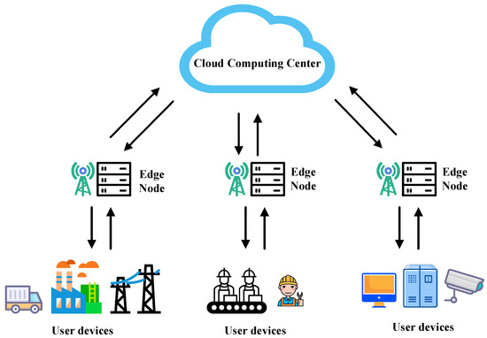
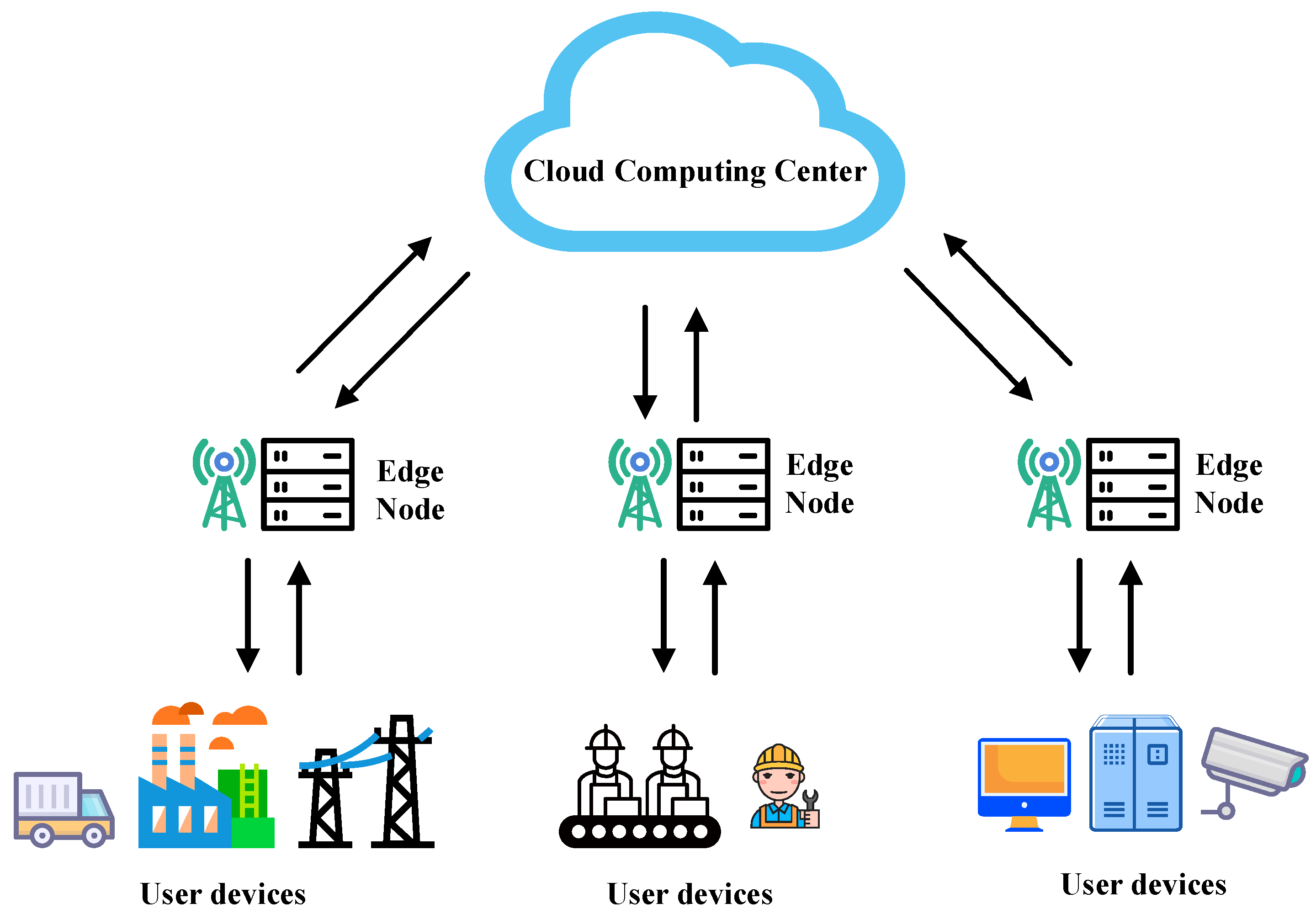
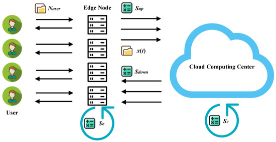
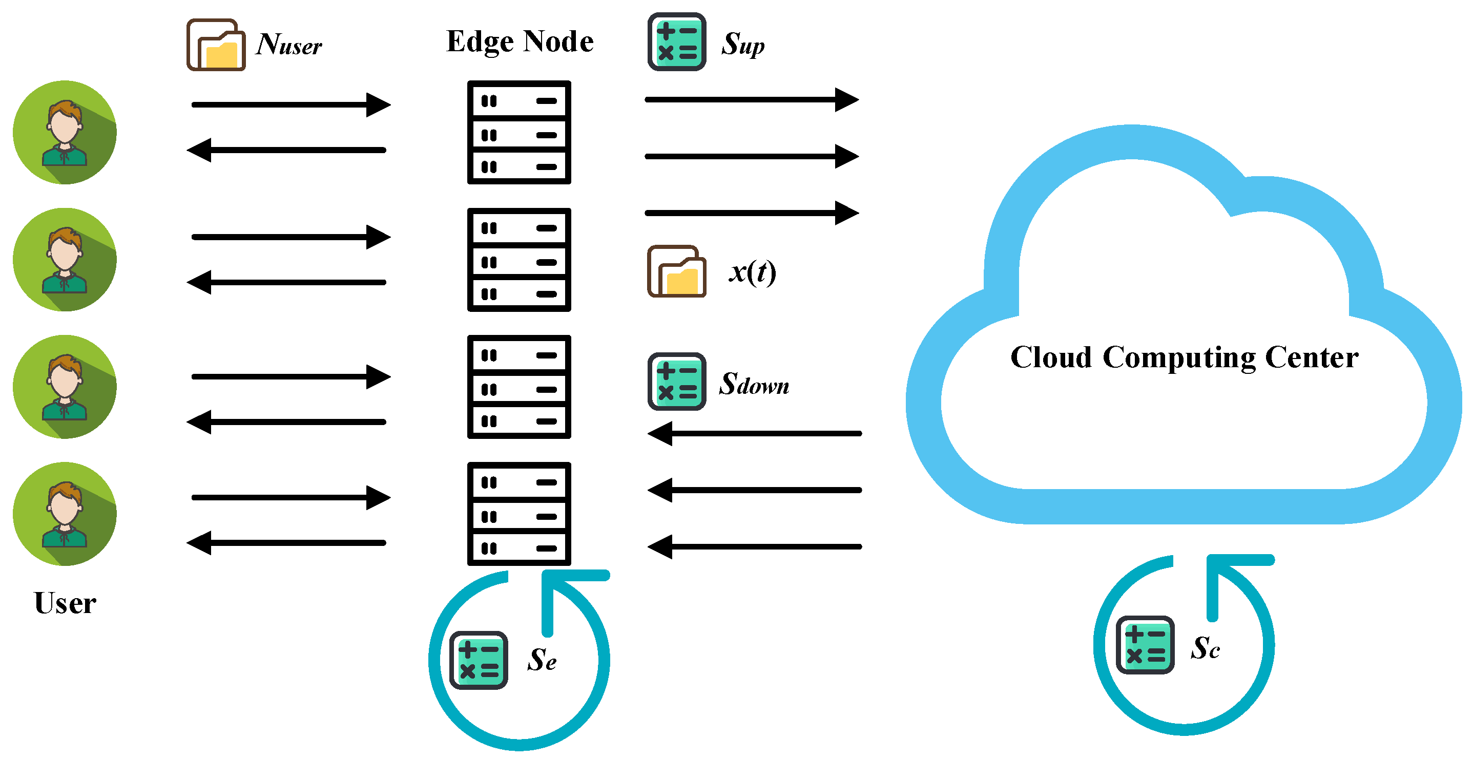
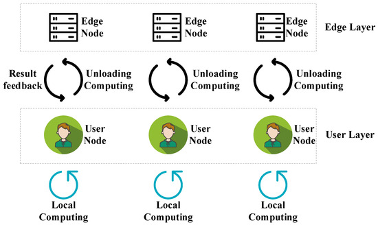
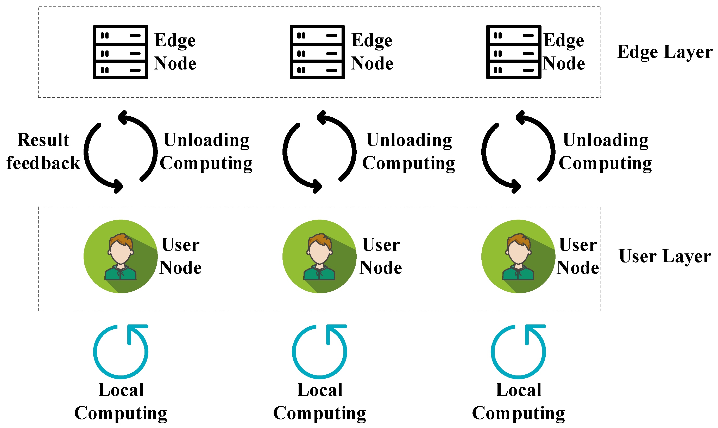
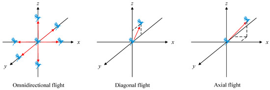
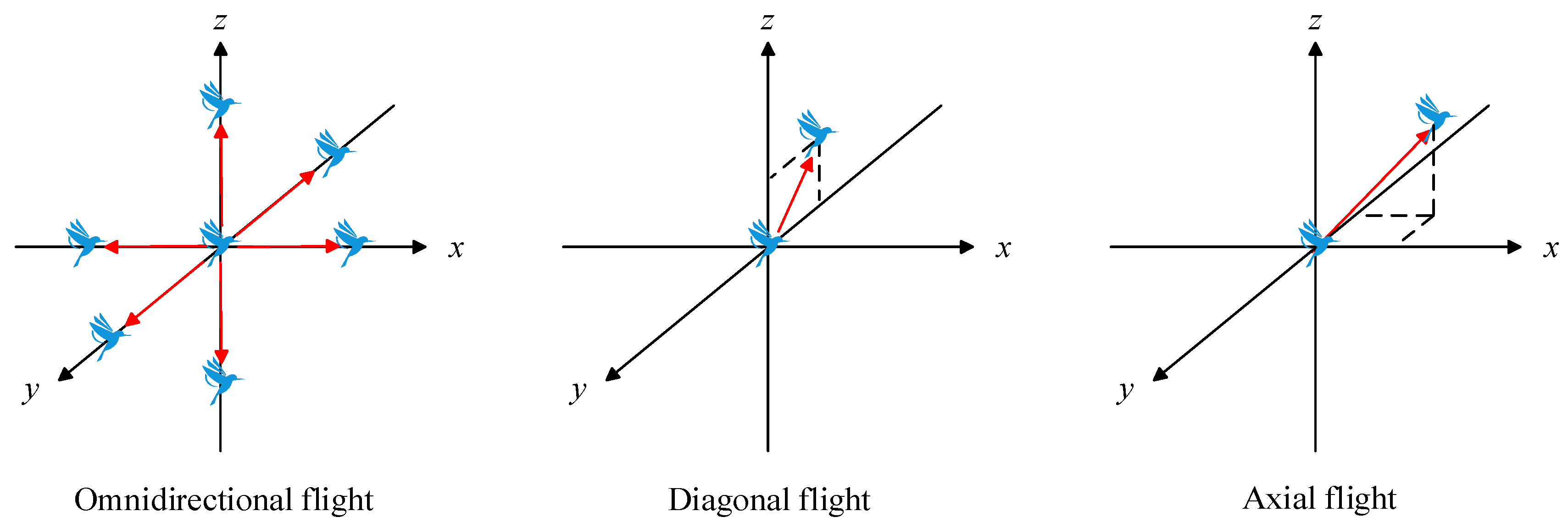
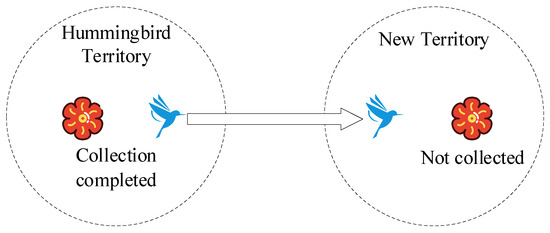
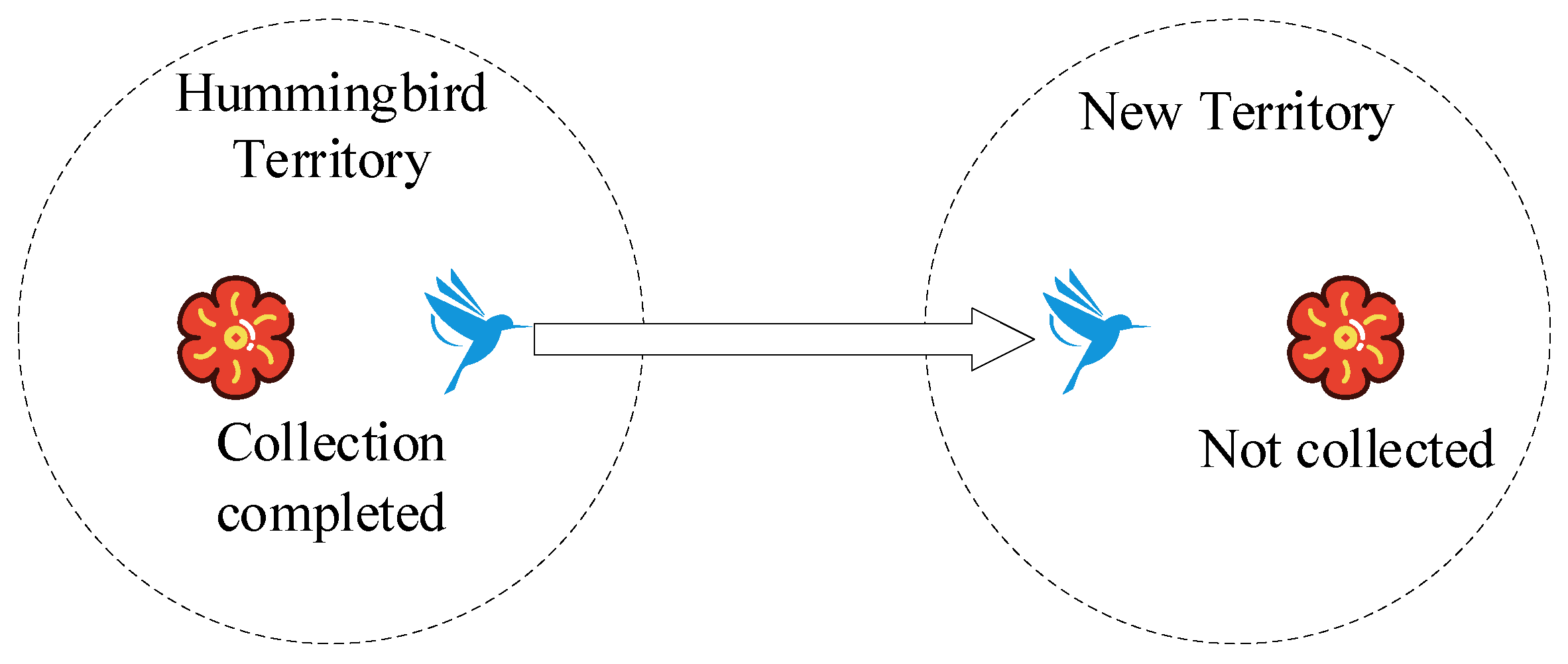
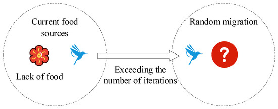
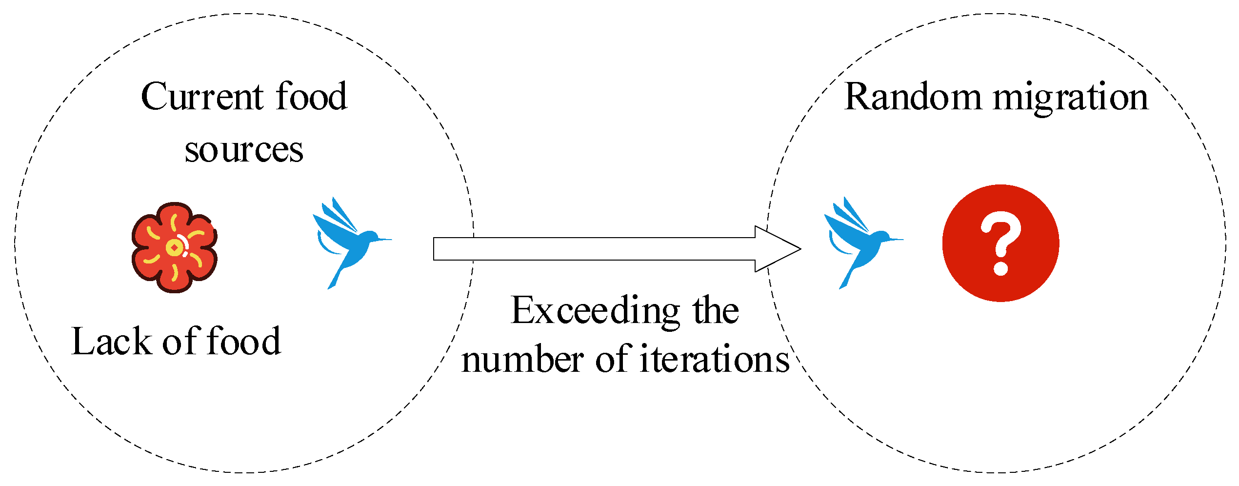
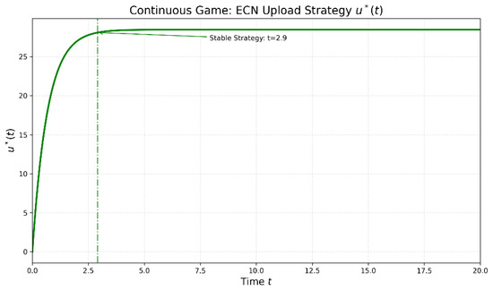
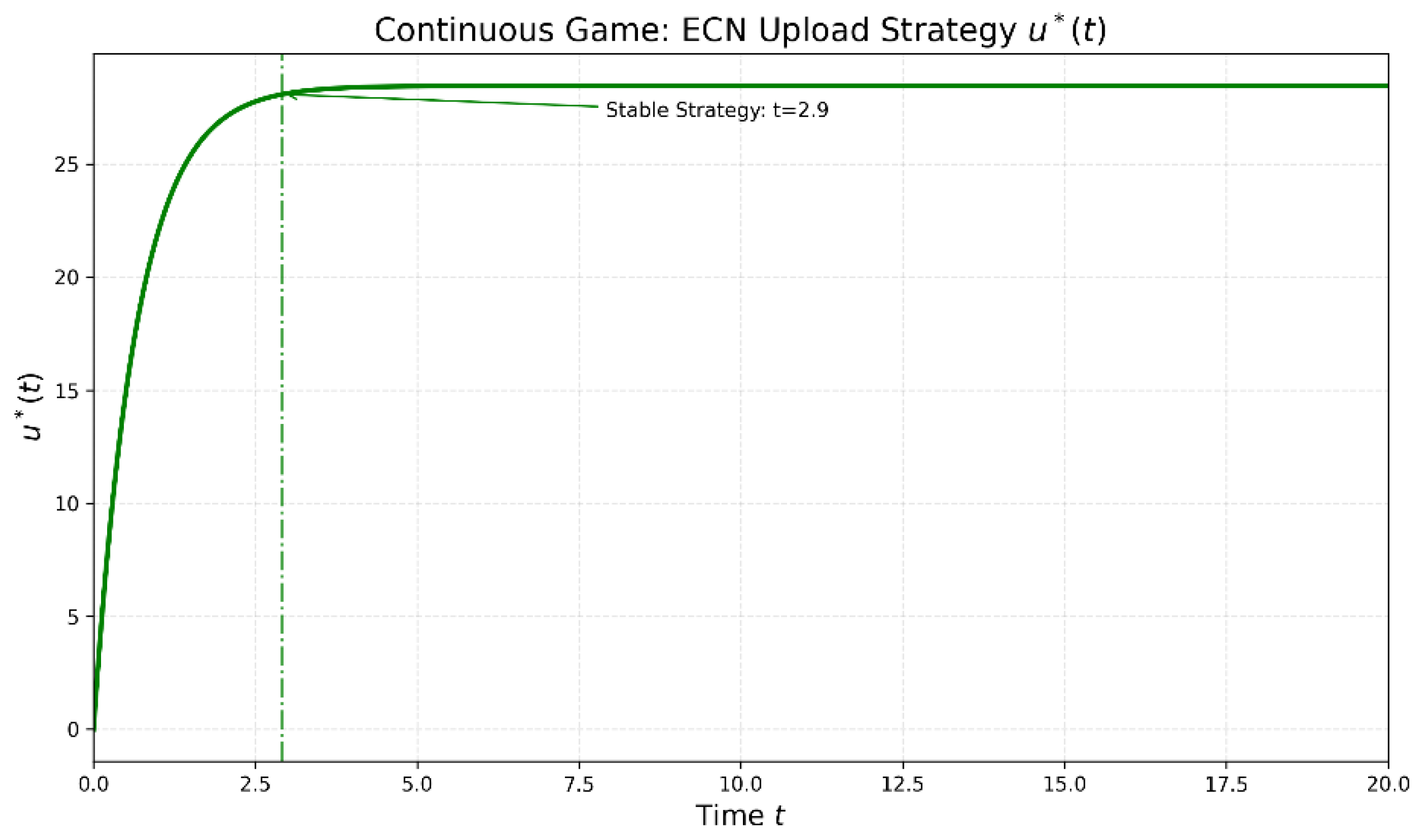
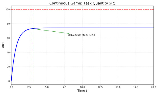
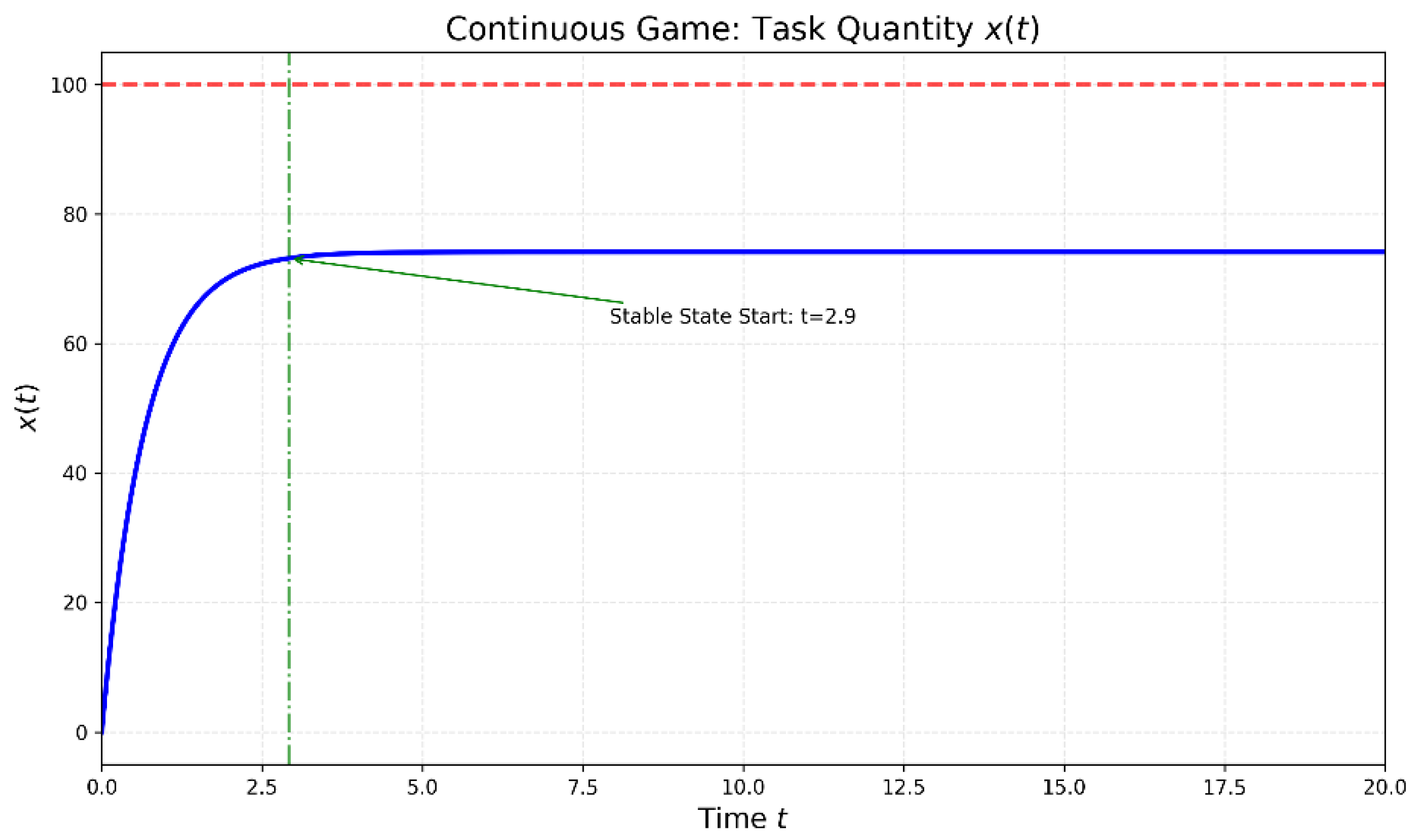
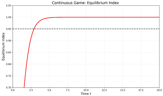
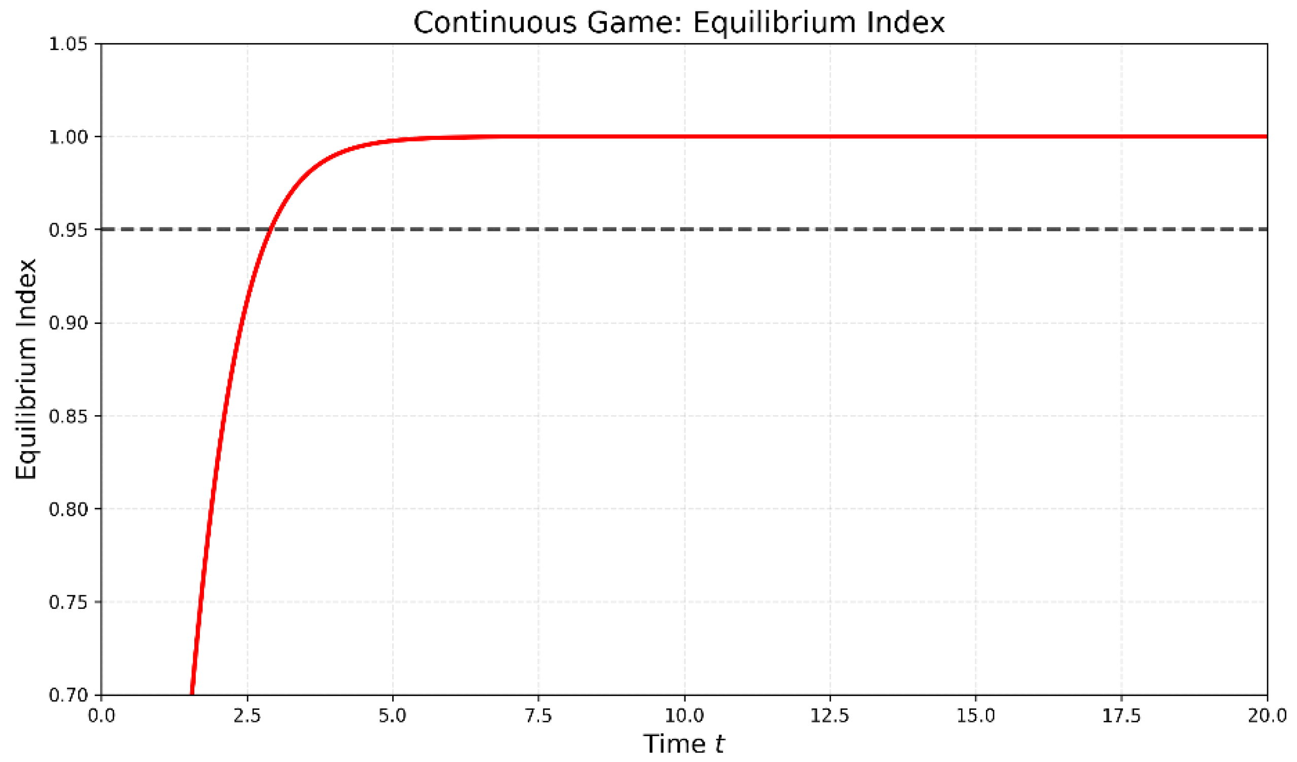
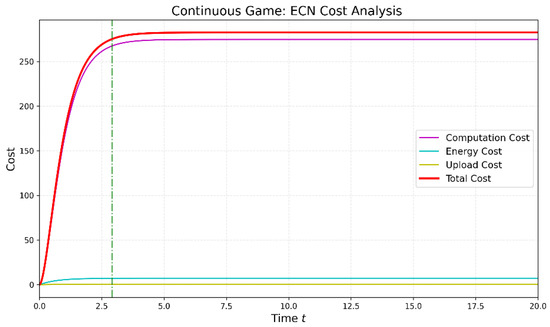
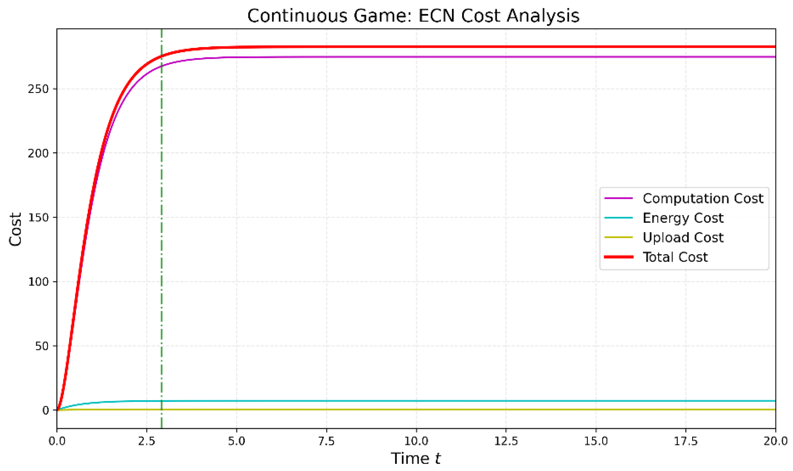
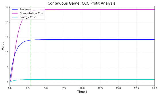
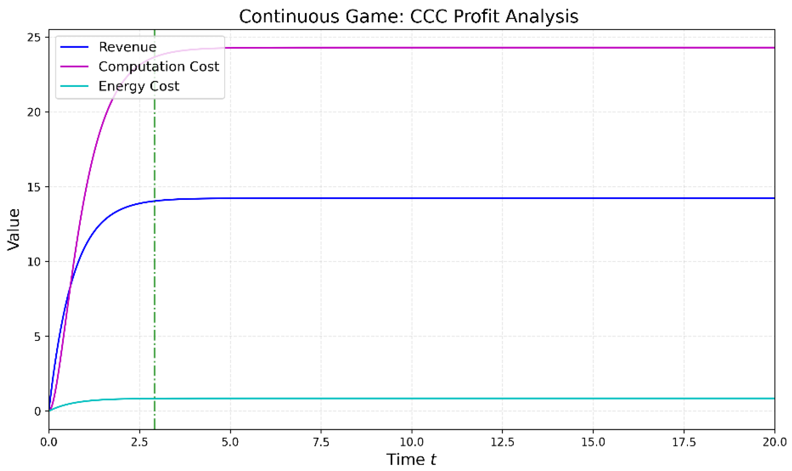
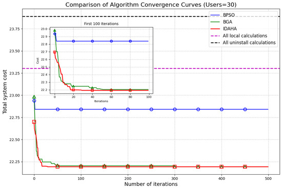
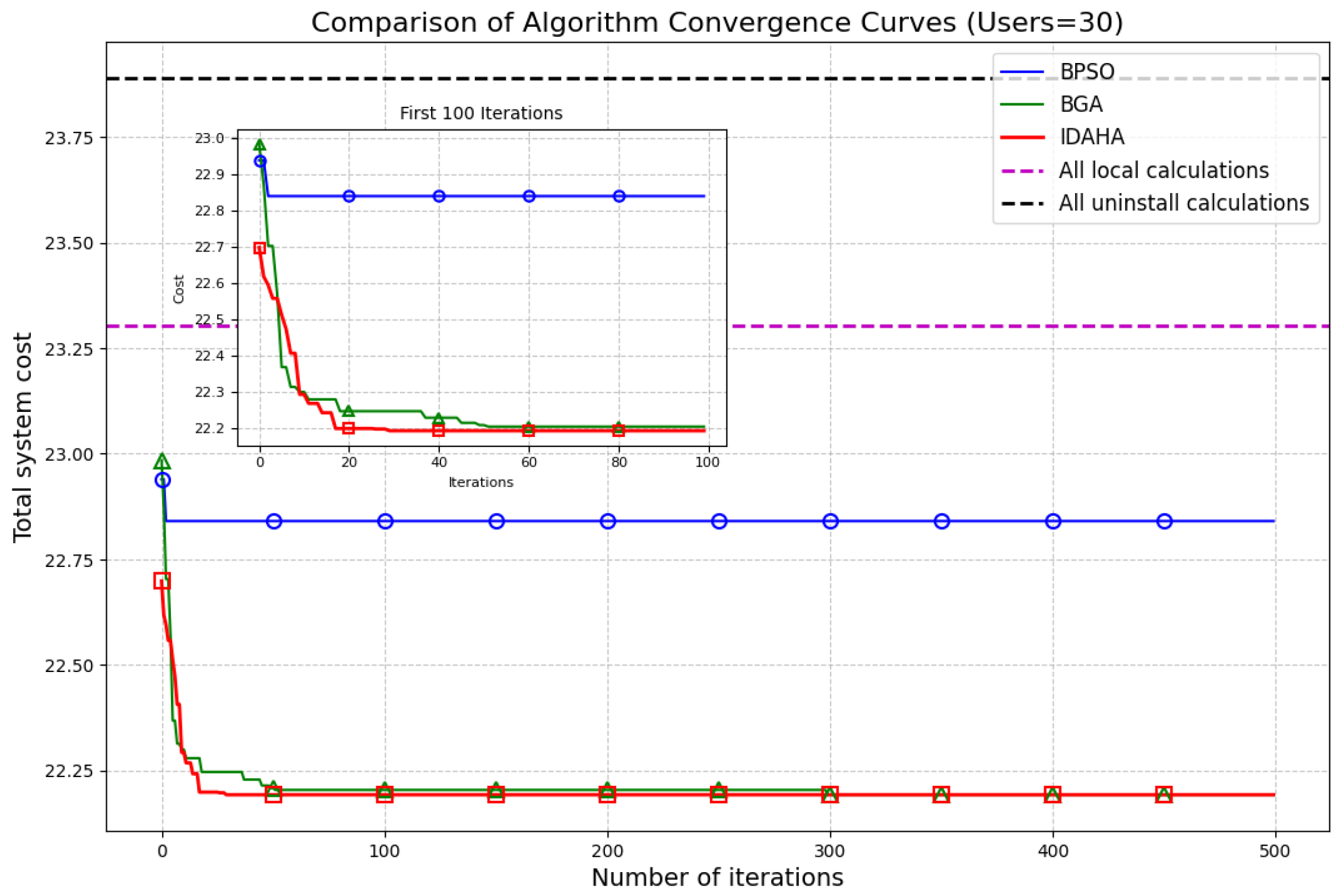
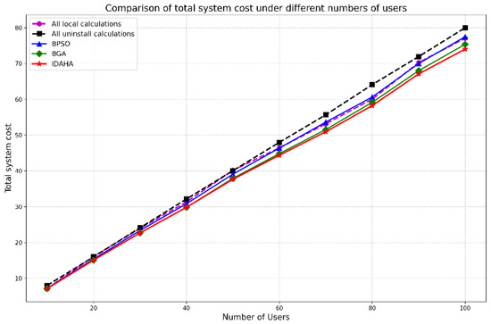
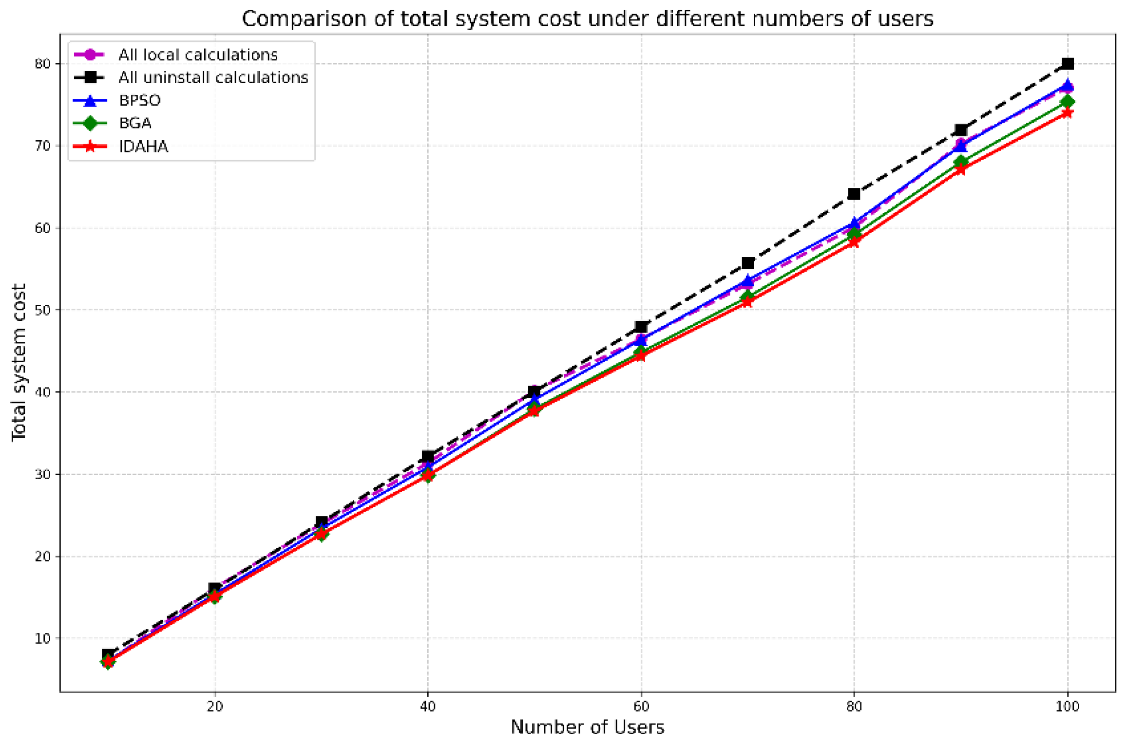
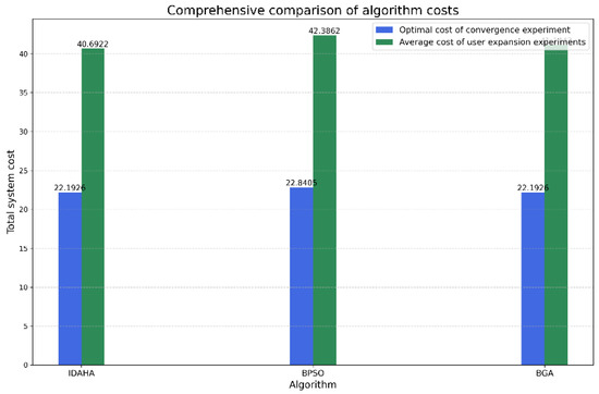
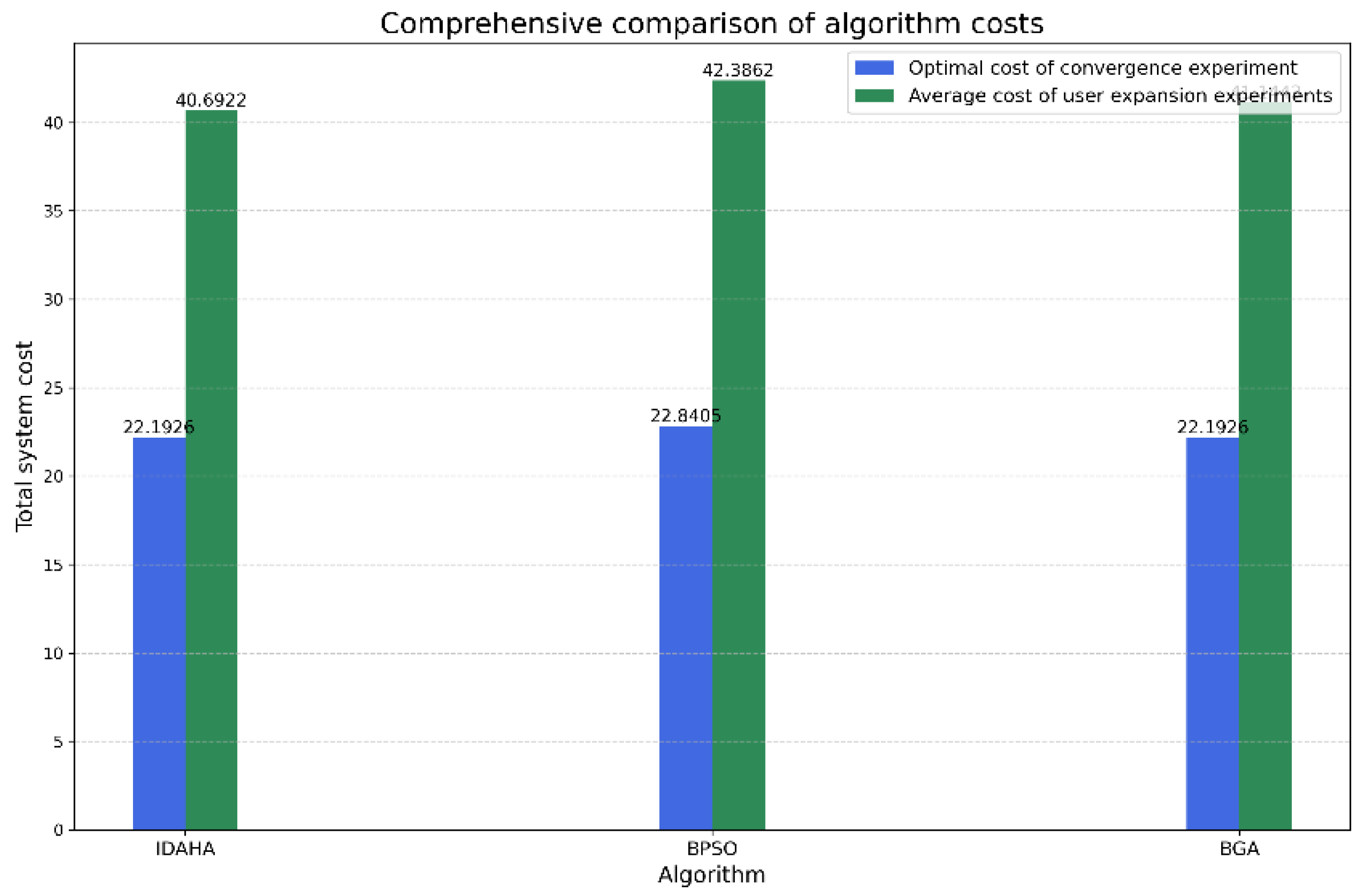
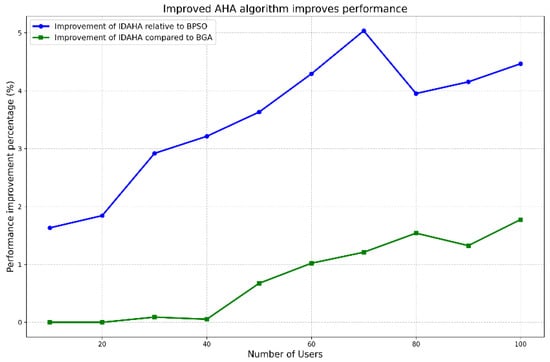
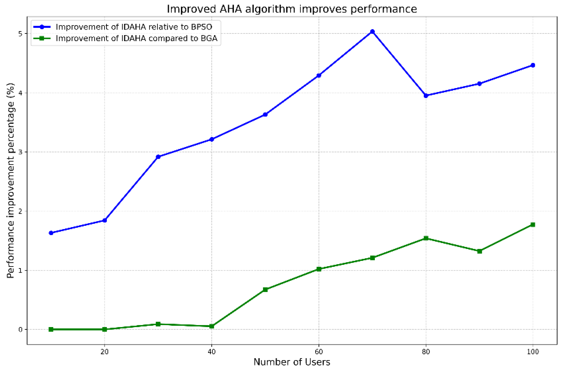
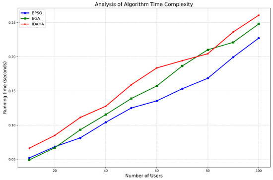
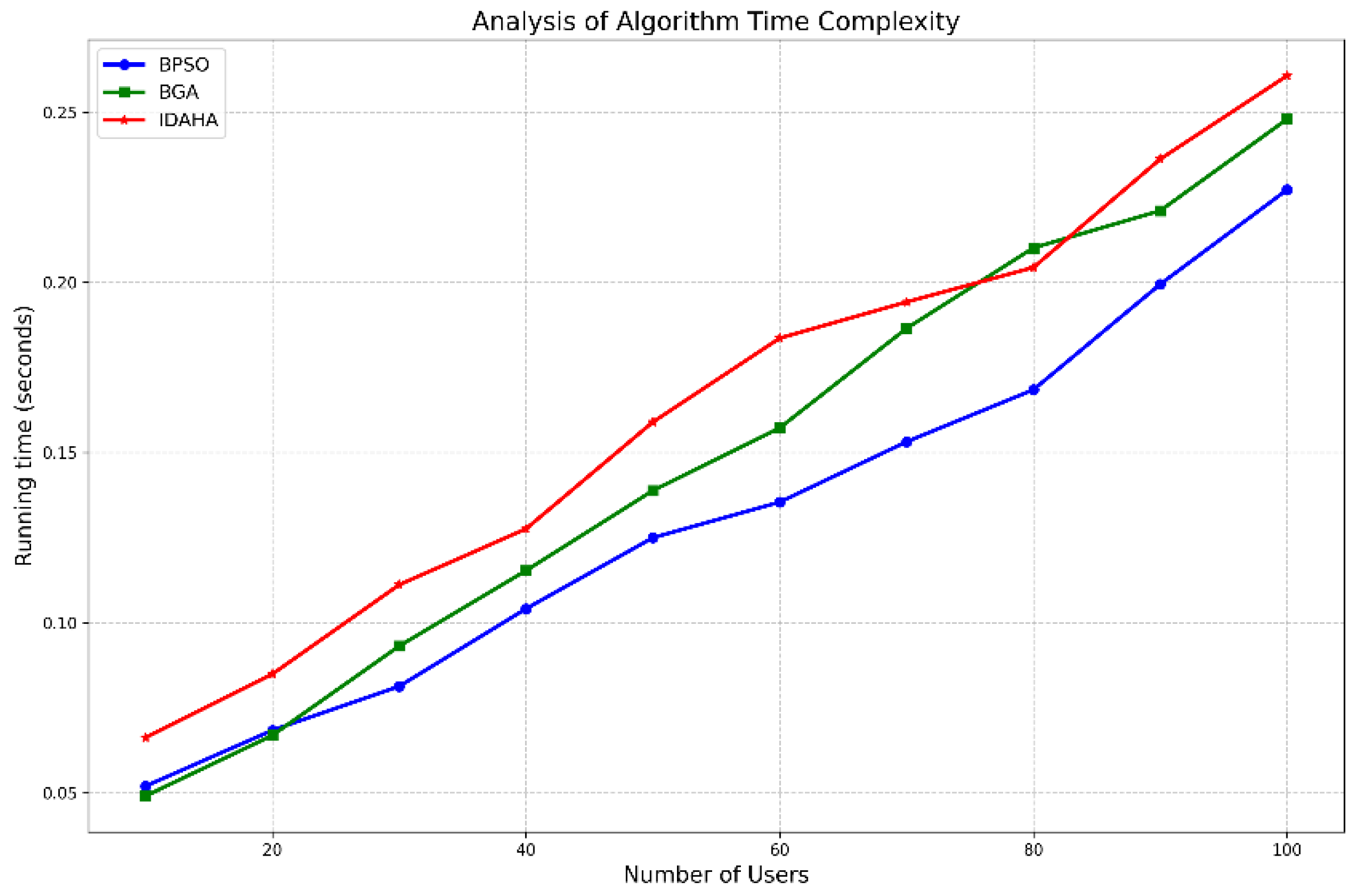
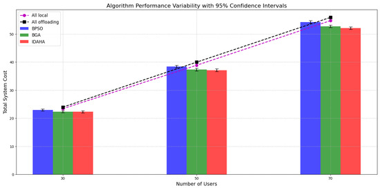
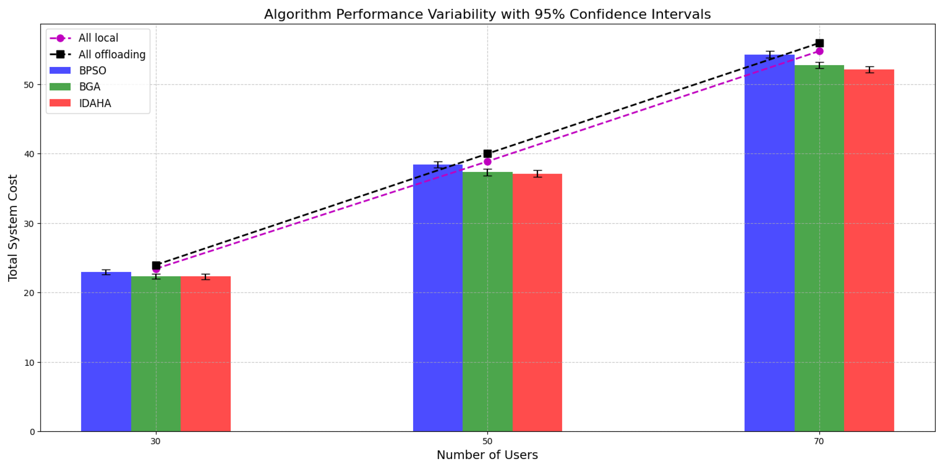
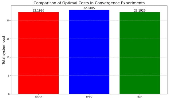
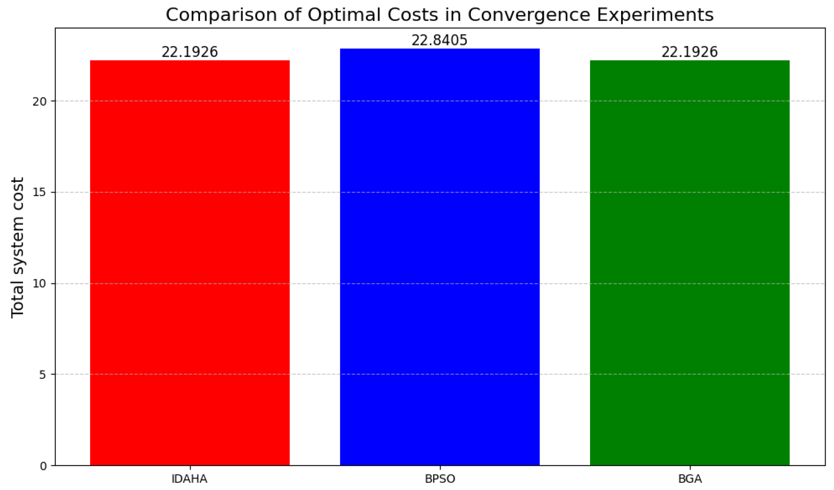
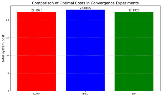
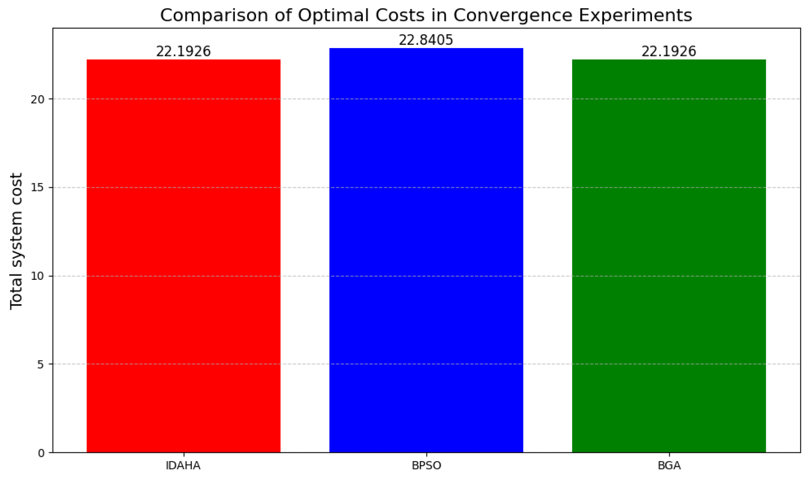
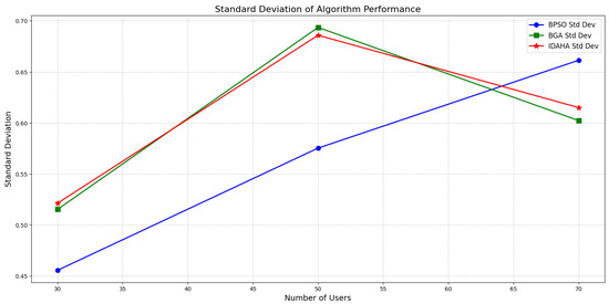
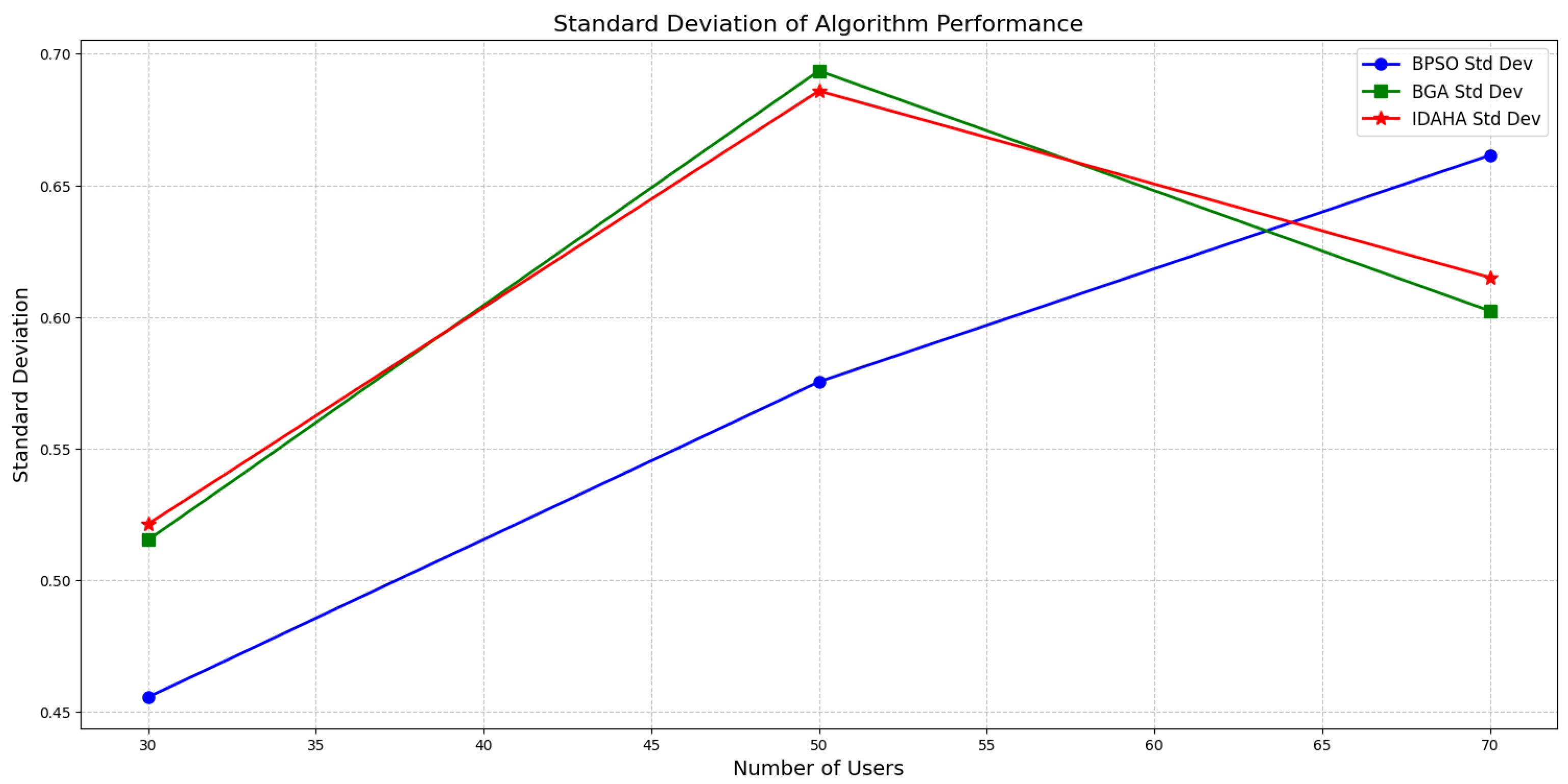

Disclaimer/Publisher’s Note: The statements, opinions and data contained in all publications are solely those of the individual author(s) and contributor(s) and not of MDPI and/or the editor(s). MDPI and/or the editor(s) disclaim responsibility for any injury to people or property resulting from any ideas, methods, instructions or products referred to in the content. |
© 2026 by the authors. Licensee MDPI, Basel, Switzerland. This article is an open access article distributed under the terms and conditions of the Creative Commons Attribution (CC BY) license.