


Abstract
Root-cause analysis (RCA) in large-scale microservice-based payment systems is challenging due to complex failure propagation along service dependencies, limited availability of labeled incident data, and heterogeneous service topologies across deployments. We propose ServiceGraph-FM, a pretrained graph-based model for RCA, where “foundation” denotes a self-supervised graph encoder pretrained on large-scale production cluster traces and then adapted to downstream diagnosis. ServiceGraph-FM introduces three components: (1) masked graph autoencoding pretraining to learn transferable service-dependency embeddings for cross-topology generalization; (2) a temporal relational diffusion module that models anomaly propagation as graph diffusion on dynamic service graphs (i.e., Laplacian-governed information flow with learnable edge propagation strengths); and (3) a causal attention mechanism that leverages multi-hop path signals to better separate likely causes from correlated downstream effects. Experiments on the Alibaba Cluster Trace and synthetic PayPal-style topologies show that ServiceGraph-FM outperforms state-of-the-art baselines, improving Top-1 accuracy by 23.7% and Top-3 accuracy by 18.4% on average, and reducing mean time to detection by 31.2%. In zero-shot deployment on unseen architectures, the pretrained model retains 78.3% of its fully fine-tuned performance, indicating strong transferability for practical incident management.
Keywords:
graph-based models; root-cause analysis; AIOps; temporal graph networks; microservice architecture; anomaly detection MSC:
68T07
1. Introduction
The proliferation of microservice architectures in modern cloud-native applications has fundamentally transformed the operational landscape of large-scale distributed systems, particularly in mission-critical domains such as online payment platforms, e-commerce infrastructures, and financial transaction processing systems [1,2]. Companies such as PayPal, Stripe, and Alipay operate service meshes composed of thousands of interconnected microservices, where individual services may process millions of transactions per second while maintaining complex dependency relationships with numerous upstream and downstream components. While this paradigm enables independent deployment and improved fault isolation, it also poses significant challenges for system reliability and failure diagnosis [3]. When anomalies occur, their effects often propagate rapidly along service dependency chains, resulting in cascading failures that obscure the true source of the problem [4]. In practice, traditional rule-based monitoring and alerting systems generate large volumes of correlated alerts, making timely and accurate root-cause identification extremely difficult for human operators.
Recent advances in Artificial Intelligence for IT Operations (AIOps) have demonstrated that machine learning techniques, particularly Graph Neural Networks (GNNs), are well suited for modeling service dependency structures and reasoning over relational data [5,6]. By operating directly on service call graphs, GNNs can capture topological relationships between services and propagate information along dependency edges. Several representative studies have applied GNN-based methods to microservice root-cause analysis (RCA), including attention-based aggregation mechanisms [7] and temporal graph convolutions for correlating anomalous metrics over time [8]. Despite their effectiveness, existing approaches suffer from three major limitations. First, most methods rely on training task-specific models from scratch for each target system, which requires substantial amounts of labeled incident data that are costly and difficult to obtain in production environments [9]. Second, many approaches treat service graphs as static or weakly dynamic structures, failing to adequately capture the spatiotemporal coupling inherent in anomaly propagation processes [10]. Third, correlation-based reasoning often struggles to distinguish true causal relationships from spurious correlations, leading to false positives in root-cause localization [11].
Motivated by the recent success of large-scale self-supervised pretraining in natural language processing [12] and computer vision [13], we investigate whether a similar pretraining-and-transfer paradigm can address the above limitations in microservice RCA. Prior work on pretrained foundation models emphasizes training on massive unlabeled datasets to obtain representations that can be adapted to downstream tasks with limited supervision [14]. In this work, we adopt this paradigm in a task-specific and restricted sense: rather than claiming broad cross-domain generality or emergent reasoning capabilities, we focus on leveraging large-scale unlabeled service interaction traces to learn transferable representations for root-cause analysis across heterogeneous service topologies. Publicly available cluster traces contain millions of service interactions under diverse workload patterns, providing an opportunity to pretrain graph encoders that capture common structural and temporal characteristics of microservice systems.
Based on this perspective, we propose ServiceGraph-FM, a graph pretraining framework tailored for root-cause analysis in large-scale payment service graphs. ServiceGraph-FM consists of three main components. First, we develop a self-supervised pretraining framework based on masked graph autoencoding [15], which learns reusable service dependency representations from heterogeneous cluster traces and enables effective zero-shot and few-shot adaptation to unseen service topologies. Second, we introduce a Temporal Relational Diffusion Module that explicitly models the spatiotemporal propagation of anomalous signals through service graphs using diffusion-based mechanisms, providing additional context for separating root causes from downstream effects. Third, we design a causal attention mechanism integrated with graph-based contrastive learning [16] to mitigate the influence of spurious correlations and improve robustness under confounding conditions.
We evaluate ServiceGraph-FM on the Alibaba Cluster Trace dataset [17] as well as synthetic PayPal-style microservice topologies. Experimental results demonstrate that the proposed approach consistently outperforms state-of-the-art baselines under both fully supervised and low-resource settings. Moreover, the pretrained model exhibits strong transferability in zero-shot and few-shot scenarios on previously unseen service graphs, supporting the effectiveness of the proposed pretraining paradigm for practical RCA deployment.
The remainder of this paper is organized as follows. Section 2 reviews related work on microservice RCA, graph neural networks for AIOps, and large-scale pretraining paradigms. Section 3 introduces preliminary concepts on service graphs and graph representation learning. Section 4 presents the detailed methodology of ServiceGraph-FM. Section 5 describes the experimental setup and evaluation results. Finally, Section 6 concludes the paper and discusses limitations and future research directions.
2. Related Works
2.1. Root-Cause Analysis in Microservice Systems
Root-cause analysis has long been studied in distributed systems, with early approaches relying on rule-based expert systems and statistical correlation analysis [18,19]. With the widespread adoption of microservice architectures, service dependency graphs have become significantly larger and more complex, increasing the difficulty of accurate and timely fault localization. Traditional methods such as dependency graph analysis [20] and correlation-based anomaly detection [21] are often effective in small-scale settings, but they tend to suffer from high false positive rates in large systems due to their limited ability to distinguish causal relationships from spurious correlations.
More recent studies have explored machine learning-based approaches for microservice RCA. Microscope [10] constructs causal graphs from distributed traces and applies PageRank-style ranking to identify likely root causes, but it requires extensive labeled data for each deployment environment. MicroRCA [8] combines random walks on service dependency graphs with time-series anomaly scores, achieving improved accuracy within individual systems but exhibiting limited generalization across different deployments. CloudRCA [7] employs graph attention networks to aggregate features from neighboring services, yet models the service graph as static and does not explicitly capture temporal anomaly propagation. Several works have also incorporated causal inference techniques, including CauseInfer [9], which applies the PC algorithm to learn causal structures from monitoring data, and AutoMAP [11], which uses attributed graph embeddings with anomaly injection for training. While these approaches improve robustness compared to purely correlation-based methods, they remain dependent on system-specific training data and are difficult to transfer to new environments. More recent efforts have explored leveraging multi-modal operational data [22] and large language models or agent-based systems [23,24] for RCA. While these LLM- and agent-based approaches have shown promise in interactive root-cause analysis, they typically operate under different assumptions, relying on extensive textual logs, tool calls, or human-in-the-loop interactions. As such, they are not directly comparable to our approach, which focuses on graph-based, automated RCA using structured monitoring and trace data under fixed inference budgets. Especially, our approach focuses on learning transferable representations through large-scale pretraining, aiming to reduce reliance on per-system supervision rather than claiming fundamentally different modeling assumptions.
2.2. Graph Neural Networks for AIOps
Graph neural networks provide a general framework for learning representations on structured data and have been successfully applied in domains such as social networks [25], molecular graphs [26], knowledge graphs [27], and wireless communication [28]. GNNs operate by iteratively aggregating information from neighboring nodes, enabling the modeling of relational dependencies in complex systems. In the context of AIOps, several works have adapted GNN architectures for operational monitoring and diagnosis tasks. Zeng et al. [29] applied graph convolutional networks (GCN) to detect KPI anomalies by constructing correlation graphs over time-series metrics. Wang et al. [30] proposed GROOT, which uses attention-based GNNs to model service invocation chains for performance diagnosis. Li et al. [31] introduced multidimensional GNNs that jointly capture service topology and metric correlations for failure prediction.
Despite these advances, most existing GNN-based AIOps methods focus on single-task optimization within a fixed system. Models are typically trained from scratch on target environments, requiring labeled data that is expensive and often unavailable in practice. Moreover, many approaches process static graph snapshots and rely on separate temporal encoders, such as recurrent networks or transformers, to handle time-series features. This separation limits their ability to capture the intrinsic spatiotemporal coupling involved in anomaly propagation. Recent work on temporal graph learning [32,33] has proposed dynamic GNN architectures with evolving node representations, but these methods have seen limited adoption in microservice RCA. Our Temporal Relational Diffusion Module is complementary to this line of research, as it explicitly models anomaly propagation over service dependencies while remaining compatible with pretrained graph representations.
2.3. Foundation Models and Transfer Learning
Foundation models, which are pretrained on large-scale datasets and adapted to downstream tasks, have shown strong transfer learning capabilities across multiple domains [14]. In natural language processing, models such as BERT [34] and GPT-3 [12] demonstrate that large-scale pretraining can significantly reduce the amount of labeled data required for downstream tasks. Similar trends have been observed in computer vision with pretrained vision transformers [13]. These successes suggest that pretraining can be an effective strategy for learning reusable representations, particularly in data-scarce settings.
Recent work has begun extending pretraining paradigms to graph-structured data. GraphMAE [15] proposed masked graph autoencoding for self-supervised graph representation learning, while GPT-GNN [35] explored pretraining graph neural networks on large-scale graphs for downstream transfer. These methods primarily focus on static graph benchmarks such as citation and social networks. In contrast, operational service graphs are dynamic, noisy, and closely tied to deployment-specific constraints. Our work builds on these graph pretraining approaches by applying them to dynamic service dependency graphs in AIOps settings. Rather than asserting universal applicability across arbitrary domains, ServiceGraph-FM aims to learn transferable representations across heterogeneous microservice systems within the same application domain, supported by pretraining on real-world cluster traces and explicit modeling of temporal dynamics.
3. Preliminaries
In this section, we provide the necessary background and formal definitions for understanding our ServiceGraph-FM framework. We introduce the mathematical formulation of service graphs, define the root-cause analysis problem, and briefly review key concepts in graph neural networks.
3.1. Service Graph Representation
A microservice system can be modeled as a directed attributed graph , where represents the set of N microservices, and denotes the set of directed edges representing service dependencies. An edge indicates that service invokes service as part of request processing. The node feature matrix contains the attributes of each service, where represents the feature vector for service , typically including metrics such as CPU utilization, memory consumption, request latency, error rate, and throughput. The adjacency matrix encodes the graph structure, where if and otherwise.
Illustrative Example. To illustrate the above representation, we consider a simplified payment microservice system consisting of five services: a frontend gateway (), an authentication service (), a payment processing service (), a fraud detection service (), and a database service (). The service dependencies form directed edges such as , , , and , indicating that incoming user requests are first handled by the gateway, then forwarded to authentication and payment services, with downstream calls to fraud detection and persistent storage. Each service node is associated with a feature vector capturing its runtime state. For example, the feature vector of the payment service may include high request latency and elevated CPU utilization during an incident, while the database service may exhibit increased queue length and error rate. Collectively, these features form the node feature matrix , while the invocation relationships define the adjacency matrix . This graph representation enables the model to reason jointly over service-level metrics and dependency structure when identifying potential root causes.
For temporal analysis, we extend this representation to a sequence of graph snapshots over time. Let denote the service graph at time step t, where the topology may evolve (e.g., due to auto-scaling or deployment changes) and node features vary according to system workload. We define the temporal service graph as , representing the system state over T consecutive time steps.
3.2. Problem Formulation
Given a temporal service graph and an anomaly detection window where system degradation is observed, the root-cause analysis task aims to identify the subset of services that are the true origins of the observed anomalies. Formally, we define anomaly indicators for each time step t, where if service exhibits anomalous behavior at time t (e.g., latency exceeding threshold, error rate spike) and otherwise.
The root-cause localization problem can be formulated as a node ranking task: given the sequence of anomaly indicators and the corresponding service graphs , we aim to learn a function , where is a score vector assigning each service a probability of being a root cause. Services are then ranked by their scores, and the top-K services with the highest scores constitute our root-cause prediction .
3.3. Graph Neural Networks Basics
Graph neural networks operate by iteratively aggregating information from neighboring nodes to compute node representations. A standard GNN layer can be expressed as:
where denotes the hidden representation of node at layer l, is the set of neighbors of , is a learnable weight matrix, is a non-linear activation function, and AGGREGATE is a permutation-invariant aggregation function (e.g., mean, max, or attention-weighted sum). The initial node representations are typically set to the input features .
In graph attention networks (GAT), the aggregation function employs attention mechanisms to weight the importance of different neighbors:
where represents the attention coefficient between nodes and at layer l, computed as:
where is a learnable attention vector and denotes concatenation. These attention mechanisms are particularly relevant for our approach, as they allow the model to dynamically focus on the most relevant service dependencies during anomaly propagation.
4. Methodology
In this section, we present the detailed design of ServiceGraph-FM, our pretrained graph-based model for root-cause analysis in microservice systems. The overall framework consists of three core components: a self-supervised pretrained graph encoder that learns universal service dependency representations, a Temporal Relational Diffusion Module that models the spatiotemporal propagation of anomalies, and a Causal Attention Mechanism integrated with contrastive learning for robust root-cause identification.
4.1. Service Graph Construction from Cluster Traces
A critical prerequisite for pretraining ServiceGraph-FM is the construction of service dependency graphs from large-scale cluster traces. Publicly available datasets, such as the Alibaba Cluster Trace, do not provide explicit microservice dependency graphs. Instead, they record fine-grained execution information, including service identifiers, invocation events, timestamps, and resource-level monitoring signals. In this work, service graphs are therefore derived from cluster traces through a trace-driven dependency reconstruction process, rather than assuming access to ground-truth architectural graphs. Specifically, each service is represented as a node, and directed edges are inferred by aggregating observed invocation relationships in distributed traces. For a given request trace, if service invokes service , we add a directed edge to the service graph. To account for temporal dynamics, edge weights are computed based on the normalized frequency of invocations within sliding time windows, reflecting both the strength and persistence of service interactions. This procedure yields a time-evolving service graph that captures dominant dependency patterns observed in production workloads. Although the resulting graphs are inferred rather than manually specified, they exhibit several properties consistent with real microservice architectures. First, the reconstructed graphs are sparse, with most services interacting with a limited number of neighbors, aligning with service decomposition principles. Second, core service dependencies remain stable across time windows, while peripheral dependencies exhibit higher temporal variability, reflecting realistic workload fluctuations. Third, anomalous signals observed in monitoring data propagate primarily along the inferred dependency paths, providing empirical support that the reconstructed graphs capture meaningful operational relationships. It is important to emphasize that the goal of this reconstruction is not to recover exact architectural diagrams, but to obtain sufficiently faithful interaction graphs that support representation learning and anomaly propagation modeling. The fidelity of the inferred graphs is indirectly validated through downstream root-cause analysis performance and transfer experiments, where models pretrained on these graphs generalize effectively to unseen service topologies.
4.2. Self-Supervised Graph Pretraining
A fundamental challenge in microservice root-cause analysis is the scarcity of labeled incident data, particularly for newly deployed systems or environments with limited operational history. To mitigate this issue, we adopt a self-supervised pretraining framework that leverages large-scale unlabeled cluster traces to learn transferable service dependency representations. This design is motivated by the observation that microservice systems often share recurring architectural patterns, such as cache-aside designs, retry mechanisms, and circuit breaker configurations, and that anomaly propagation dynamics exhibit common structural characteristics across different workloads.
Given a service graph constructed from cluster traces, we perform masked graph autoencoding to learn node representations that capture both service-level attributes and dependency structures. Specifically, a subset of nodes is randomly selected according to a masking ratio , and their feature vectors are replaced with a learnable mask token . The masked graph is denoted as , where:
The masked graph is processed by a multi-layer graph attention network encoder, producing node embeddings . A decoder network is then used to reconstruct the original features of the masked nodes. The pretraining objective consists of a feature reconstruction loss and a structural reconstruction loss:
where the feature reconstruction loss is defined as:
Here, denotes a decoder network that reconstructs the original node features from the learned embeddings during masked graph pretraining. The structural reconstruction loss encourages preservation of dependency relationships:
where denotes negative edge samples and is the sigmoid function. The dot product in Equation (7) measures embedding similarity and is used to approximate graph adjacency, as commonly done in graph embedding and link prediction objectives. Thus, maximizing this similarity for connected node pairs encourages the learned representations to preserve the underlying service dependency topology.
In addition to node-level masking, we introduce edge masking by randomly removing a subset of dependency edges and training the model to predict their existence based on learned node embeddings. This joint masking strategy encourages the encoder to capture both local service characteristics and higher-order dependency patterns, which are essential for effective transfer to downstream RCA tasks.
Realism of the Masking Strategy. Unlike purely random masking schemes, our masking strategy is designed to reflect partial observability in real operational systems. In practice, service monitoring data may be incomplete due to missing metrics, delayed logs, or transient monitoring failures. To mimic these conditions, masking is applied locally within short temporal windows and restricted neighborhoods, rather than uniformly across the entire graph. As a result, the model is trained to infer service states from contextual information provided by neighboring services and recent history, aligning the pretraining objective with realistic diagnostic scenarios.
4.3. Temporal Relational Diffusion Module
Standard GNN architectures process service graphs as static snapshots, treating temporal dynamics through separate sequential models that operate independently from spatial aggregation. This decoupled approach fails to capture the fundamental characteristics of anomaly propagation: failures diffuse through service dependencies over time, with propagation patterns determined by the graph structure. To address this limitation, we propose the Temporal Relational Diffusion Module, which models anomaly states as diffusing quantities that flow through the service graph according to learned diffusion dynamics.
The key insight of our diffusion framework is that anomaly propagation can be modeled as a continuous diffusion process governed by the heat equation on graphs. Consider the anomaly state vector at time t, where represents the anomaly intensity of service . The evolution of this state over time follows a diffusion process:
where is the graph Laplacian, is the degree matrix, and is a learned weighted adjacency matrix that encodes the propagation strength along each edge. Unlike the binary adjacency matrix , the weights in are learned to reflect the actual anomaly transmission rates between services, capturing factors such as timeout configurations, connection pool sizes, and circuit breaker thresholds.
To compute the diffusion weights, we introduce an edge feature extraction mechanism that considers both the temporal patterns of service interactions and the structural importance of each dependency. For each edge , we extract edge features that encode the historical correlation between services and , including metrics such as average call frequency, typical latency distribution, and co-occurrence patterns in past incidents. As a concrete example, consider a dependency edge from an upstream authentication service to a downstream payment service. The corresponding edge feature vector may include (i) the average request rate between the two services over a recent time window, (ii) the mean and variance of observed request latency, and (iii) the frequency with which anomalies in the upstream service are followed by anomalies in the downstream service. Together, these features provide a data-driven summary of both interaction strength and historical anomaly coupling, which the model uses to learn diffusion weights that reflect realistic propagation behavior. The diffusion weight is then computed as:
where MLPw denotes a multi-layer perceptron that maps the concatenated features to a scalar weight value, and are the node embeddings from the pretrained encoder.
The discrete-time diffusion dynamics can be approximated through matrix exponential:
where is the time step size. However, computing matrix exponential directly is computationally expensive for large graphs. We therefore adopt a polynomial approximation based on Chebyshev polynomials, which provides an efficient implementation while maintaining expressiveness:
where denotes the k-th order Chebyshev polynomial, is the rescaled Laplacian, is the largest eigenvalue of , and are learnable coefficients.
The, Temporal Relational Diffusion Module can be intuitively understood as modeling how anomalies propagate through service dependencies with different strengths and delays. In a microservice system, not all dependencies transmit anomalous effects equally: for example, a synchronous RPC call with tight timeout constraints may propagate failures rapidly, while an asynchronous message queue or a cached dependency may attenuate or delay anomaly transmission. The learned diffusion weights capture these heterogeneous propagation characteristics directly from data. Concretely, the diffusion weight associated with an edge reflects how strongly and how quickly anomalies observed at an upstream service are likely to influence downstream services. These weights are learned from historical interaction patterns and anomaly correlations, allowing the model to distinguish high-impact dependency paths from weak or incidental connections. During inference, anomaly signals diffuse along the service graph following these learned weights, causing services that lie on strong propagation paths to accumulate higher anomaly influence, while services connected through weak or indirect paths receive attenuated signals. From this perspective, diffusion weight learning and anomaly propagation are tightly coupled: learning accurate diffusion weights determines how anomaly evidence flows through the graph, and effective propagation enables the model to separate true root causes from downstream effects. This allows ServiceGraph-FM to move beyond static correlation by explicitly modeling how failures spread across service dependencies over time.
Furthermore, to incorporate the rich temporal information from monitoring metrics, we augment the diffusion process with a temporal attention mechanism. At each time step, we compute attention scores over historical states to determine which past observations are most relevant for predicting current anomaly propagation:
where are query and key matrices derived from current and historical node embeddings through linear transformations. The temporally attended state is then computed as:
where contains the value representations of historical states. The final propagated state combines both the diffusion dynamics and temporal attention:
where is a learnable gating parameter that balances the contribution of spatial diffusion and temporal attention.
4.4. Causal Attention for Root-Cause Identification
A critical challenge in root-cause analysis is distinguishing genuine causal relationships from spurious correlations. Two services may exhibit correlated anomalies due to common upstream dependencies, shared infrastructure resources, or coincidental timing, yet only one may represent the true root cause. Standard attention mechanisms in GNNs can learn to weight neighbors based on correlation patterns, but they lack explicit mechanisms for causal reasoning. To address this limitation, we introduce a causal attention mechanism that explicitly models intervention-based causality.
The key motivation behind our causal attention design is Pearl’s notion of interventional causality: a variable X causally affects Y if intervening on X changes the distribution of Y. In the context of service graphs, service is a causal ancestor of if an anomaly originating at (even when is not directly connected to ) leads to observable effects at through dependency chains. To capture this notion, we compute causal attention scores that reflect the expected impact of intervening on each service’s state.
Given node embeddings at time t and the current anomaly state , we compute causal attention coefficients that quantify how much service contributes to the anomaly state of service . Unlike standard attention that operates on local neighborhoods, causal attention considers multi-hop paths in the dependency graph to capture transitive causal relationships. We define:
where is a scoring function and represents path-based features that encode the structural relationship between and , including the shortest path length, the number of alternative paths, and the aggregated edge weights along the most probable path. The scoring function is implemented as:
where are learnable projection matrices. Here, the path-based features used in causal attention, such as shortest path length and aggregated edge weights, are derived from the inferred service graphs constructed from monitoring and trace data (Section 4.1). These features do not rely on static architectural diagrams, but are computed on time-evolving service graphs within each analysis window. Specifically, shortest paths are computed using the current graph snapshot, and edge weights reflect recent interaction strength inferred from invocation frequency and temporal correlation metrics. Under dynamic topologies, where services may appear or disappear over time, path features are recomputed for each time window based on the available graph structure. This design ensures that causal attention adapts to topology changes without assuming persistent global connectivity. While path features may be noisy under partial observability, they provide coarse-grained structural cues that are sufficient for regularizing attention toward plausible dependency pathways, rather than serving as precise causal estimates.
To further enhance causal reasoning, we integrate counterfactual augmentation into our training procedure. For each training sample with a known root cause , we generate counterfactual graphs by perturbing edges that are unlikely to participate in the causal chain from to observed anomalous services. Specifically, we identify edges where neither nor lie on any path from to anomalous services, and randomly remove or modify these edges. The model is trained to maintain consistent root-cause predictions across these counterfactual variations, encouraging it to focus on true causal pathways rather than spurious structural correlations.
4.5. Graph Contrastive Learning Objective
To improve the robustness and generalization of learned representations, we employ graph contrastive learning that encourages the model to learn invariant features across different manifestations of the same root cause. The core idea is that multiple incident scenarios caused by the same root service should yield similar representations, while incidents with different root causes should be distinguishable in the embedding space.
We construct positive pairs by generating two augmented views of the same incident graph using semantics-preserving transformations that do not alter the underlying root-cause label. Specifically, we apply two classes of stochastic augmentations: node feature perturbation and topology augmentation. For node feature perturbation, we add zero-mean Gaussian noise with a small variance to service-level metrics (e.g., latency, throughput, or resource utilization), ensuring that the relative ordering and anomaly patterns across services are preserved. For topology augmentation, we randomly drop a small fraction of edges that are identified as non-critical based on low diffusion weights, so that key dependency paths involved in anomaly propagation remain intact. Formally, given an incident graph associated with a root cause , we independently sample two augmentation functions and to generate two correlated views and . These two graphs share the same causal semantics and root cause, but differ in surface-level realizations of metrics and graph structure. The augmented graphs are then encoded by the graph encoder to obtain node embeddings and , which are further aggregated into graph-level representations and . The READOUT function can be implemented using mean pooling, max pooling, or attention-based aggregation, depending on the experimental setting.
The contrastive loss encourages agreement between the two augmented views:
where sim denotes cosine similarity, is a temperature parameter, B is the batch size, and is an indicator function. This objective pushes the model to learn representations that are invariant to semantics-preserving augmentations while being discriminative across different incidents.
4.6. Root-Cause Scoring and Final Prediction
The final root-cause scoring combines information from the pretrained encoder, diffusion dynamics, and causal attention. For each service , we compute a root-cause score that reflects both its intrinsic anomaly likelihood and its causal influence on the observed system-wide anomalies. The score is computed as:
where is the final node embedding at time T, is the diffused anomaly state, the third term captures the aggregated causal influence of on all services weighted by causal attention coefficients, and is a learnable weight vector. Services are ranked by their scores in descending order, and the top-K services constitute the final root-cause prediction.
4.7. Training Objective
The overall training objective of ServiceGraph-FM combines multiple loss components. For labeled incident data in the downstream RCA task, we employ a ranking loss that encourages the true root cause to be ranked higher than non-root-cause services:
where denotes the set of true root causes and is a margin hyperparameter. The complete training objective integrates the ranking loss with the contrastive learning objective:
where balances the two objectives. During pretraining, only is optimized, while during fine-tuning on downstream tasks, is used with the pretrained encoder weights serving as initialization.
4.8. Overall Algorithm
Algorithm 1 summarizes the complete workflow of ServiceGraph-FM for root-cause analysis. The algorithm takes as input a temporal service graph and anomaly indicators, and outputs ranked root-cause predictions.
| Algorithm 1 ServiceGraph-FM for Root-Cause Analysis |
| Require: Temporal service graph , anomaly indicators , pretrained encoder |
| Ensure: Root-cause ranking scores |
|
5. Experiments
In this section, we present comprehensive experimental evaluations of ServiceGraph-FM on real-world and synthetic datasets. We compare our approach against state-of-the-art baselines, conduct ablation studies to validate the contribution of each component, and analyze the model’s robustness under various perturbation scenarios.
5.1. Datasets
We evaluate ServiceGraph-FM on two primary datasets that represent different operational scales and characteristics of microservice systems.
Alibaba Cluster Trace. The Alibaba Cluster Trace dataset [17] contains production workload data collected from a large-scale cluster spanning 12 h with over 4000 machines and 12,000 containers. The dataset includes task dependency relationships, resource utilization metrics (CPU, memory, disk I/O, network bandwidth), and task execution traces. As the dataset does not provide explicit microservice dependency graphs, we derive service graphs from invocation and task dependency traces following the trace-driven reconstruction process described in Section 3.1. In the constructed graphs, nodes represent containerized services and edges denote inferred service dependencies aggregated from execution traces over temporal windows. To generate labeled root-cause scenarios, we identify real anomaly periods in the dataset characterized by resource exhaustion, abnormal latency, or task failures. For each anomaly period, we perform dependency-based backtracking over the inferred service graph to identify services that are most likely to have initiated the observed anomalous behaviors. This process yields 847 labeled incident scenarios with an average of 342 services per graph and a mean of 4.2 anomalous services per incident. Each scenario is associated with 1–3 candidate root-cause services inferred through dependency analysis. While these labels are not manually annotated ground truth, they provide a consistent and reproducible basis for comparative evaluation, following common practice in prior RCA studies on cluster traces.
Synthetic PayPal-Style Topology. To evaluate generalization to payment service architectures with controlled ground truth, we construct synthetic microservice topologies based on documented design patterns from payment processing systems [36]. The synthetic dataset models a three-tier architecture consisting of frontend services (authentication, session management, user interface), business logic services (payment processing, fraud detection, transaction validation, account management), and backend services (databases, cache layers, message queues, external payment gateways). The resulting topology contains 156 services with 423 directed dependencies. We inject realistic fault scenarios including database query slowdowns, cache misses causing cascading requests, circuit breaker triggers, and timeout propagation. Each fault scenario is simulated using queuing theory models that explicitly account for request arrival rates, service times, and queue saturation dynamics. Metric traces are synthesized with additive Gaussian noise (signal-to-noise ratio between 15–25 dB) to emulate production monitoring environments. In total, we generate 500 fault injection scenarios with controlled root causes, which serve as ground-truth labels for quantitative evaluation. We note that the synthetic fault scenarios primarily focus on queuing-theory-driven failure modes, such as slow database queries, cache breakdowns, and timeout propagation, which induce gradual or structured anomaly diffusion along service dependencies. Other common fault types, including configuration errors, low-level resource contention (e.g., CPU contention), and network partitions, are not explicitly simulated in the current synthetic dataset. These fault modes often exhibit different manifestation patterns or operate at finer system layers, and incorporating them represents an important direction for extending the fault generation framework.
Randomness Control and Reproducibility. Fault injection in the synthetic dataset follows a randomized but fully reproducible procedure. Root-cause services are sampled from eligible nodes, and fault propagation parameters are drawn from predefined distributions. All random processes are governed by fixed random seeds specified in the experimental configuration files, ensuring that the synthetic datasets and evaluation results can be exactly reproduced.
Pretraining Corpus and Code Availability. For self-supervised pretraining, we utilize both the complete Alibaba Cluster Trace dataset and the publicly available Google Cluster Data [37], which provides an additional 29 days of traces from a 12,500-machine cluster. The combined pretraining corpus contains approximately 2.3 million service interaction patterns across diverse workload types. To facilitate reproducibility, we will release scripts for converting cluster traces into service graphs, generating synthetic microservice datasets, and injecting fault scenarios, together with configuration files specifying preprocessing steps and random seeds, upon publication.
5.2. Baseline Methods
We compare ServiceGraph-FM against six state-of-the-art root-cause analysis methods:
MicroRCA [8] is a random walk-based approach that combines service dependency graphs with anomaly scores to identify root causes through personalized PageRank. The method iteratively propagates anomaly scores through the graph and ranks services by their stationary probabilities.
CloudRCA [7] employs graph attention networks to aggregate features from neighboring services and uses a multi-layer perceptron for root-cause classification. The model processes static graph snapshots with LSTM-encoded time-series features.
CauseInfer [9] applies the PC algorithm for causal discovery to learn causal relationships from monitoring metrics, then uses the learned causal graph to identify root causes through probabilistic inference.
CIRCA [38] (Causal Inference for RCA) combines random walk with causal inference by first constructing a weighted graph based on Granger causality tests, then applying diffusion processes to rank potential root causes.
GDN [39] (Graph Deviation Network) models service dependencies as a graph and detects anomalies by learning the deviation patterns between normal and abnormal states using graph neural networks with forecasting objectives.
AutoMAP [11] constructs attributed graphs augmented with anomaly indicators and trains a GCN-based model with synthetic fault injection for semi-supervised root-cause localization.
All baseline methods are implemented following their original papers and tuned with grid search over their hyperparameters to ensure fair comparison.
5.3. Evaluation Metrics
We employ multiple metrics to comprehensively assess root-cause localization performance:
Top-K Accuracy (A@K) measures the proportion of incidents where at least one true root cause appears in the top-K ranked services. We report A@1, A@3, and A@5 to reflect different operational scenarios where operators may investigate multiple candidates.
Mean Average Precision (MAP) computes the average precision across all incidents, accounting for the ranking quality of all true root causes. For an incident with ground truth root causes , the average precision is defined as:
where is the precision at position k and indicates whether the service at rank k is a true root cause.
Mean Time to Detection (MTTD) measures the average time elapsed from anomaly onset to successful root-cause identification. Lower MTTD indicates faster diagnosis, which is critical for minimizing service disruption.
False Positive Rate (FPR) quantifies the proportion of incorrectly identified root causes among the top-K predictions, providing insight into the reliability of the model’s predictions in production settings.
5.4. Experimental Setup
All experiments are conducted on a computing cluster with NVIDIA A100 GPUs (40 GB memory). For the pretraining phase, we train the graph encoder for 200 epochs with a batch size of 64 graphs. The encoder consists of 4 graph attention layers with 256 hidden dimensions and 8 attention heads. The masking ratio for node features is set to 0.3, and edge masking ratio is 0.2. For downstream RCA tasks, we fine-tune the pretrained model for 50 epochs with a learning rate of 0.0001 using the Adam optimizer. The temporal window length T is set to 30 time steps (corresponding to 5 min with 10-s granularity), and the diffusion process uses Chebyshev polynomial order . We perform 5-fold cross-validation on both datasets and report mean values with standard deviations to account for random variations in data splits and model initialization.
To simulate realistic deployment scenarios, we introduce controlled perturbations in the test data including random metric noise (±10–20% Gaussian noise), missing data points (5–15% random dropout), and topology changes (adding or removing 3–8% of edges to simulate auto-scaling or redeployment events). These perturbations reflect real-world challenges such as monitoring system glitches, network issues, and dynamic system evolution.
5.5. Overall Performance Comparison
Table 1 presents the overall performance comparison of ServiceGraph-FM against baseline methods on both datasets. Our approach achieves substantial improvements across all metrics, with particularly strong performance on Top-1 and Top-3 accuracy, which are most relevant for practical root-cause diagnosis where operators prioritize investigating the highest-ranked candidates.
Table 1.
Overallperformance comparison on root-cause localization. Best results are in bold, second best are underlined. Values represent mean ± standard deviation over 5-fold cross-validation.
On the Alibaba Cluster Trace dataset, ServiceGraph-FM achieves 62.2% Top-1 accuracy, representing a 23.7% relative improvement over the best baseline (AutoMAP at 50.3%). The improvements are consistent across all metrics, with Top-3 accuracy reaching 84.3% and MAP of 74.1%. Similar trends are observed on the PayPal-Style Topology, where our method achieves 59.7% Top-1 accuracy compared to AutoMAP’s 47.9%, demonstrating effective generalization to different architectural patterns. The standard deviations across folds are relatively small (typically 1.5–2.5%), indicating stable performance across different data splits and accounting for random variations in graph structure and anomaly patterns.
Traditional methods like MicroRCA and CauseInfer show weaker performance, primarily due to their reliance on hand-crafted features and inability to capture complex propagation patterns. CloudRCA and GDN, despite using neural network architectures, are limited by their treatment of graphs as static structures. AutoMAP benefits from synthetic fault injection during training but still requires substantial system-specific data. In contrast, ServiceGraph-FM’s pretrained representations and explicit temporal-spatial modeling enable superior performance even with limited fine-tuning data.
5.6. Ablation Study
To validate the contribution of each component in ServiceGraph-FM, we conduct comprehensive ablation studies by systematically removing or replacing key modules. Table 2 presents the results.
Table 2.
Ablation study results on Alibaba Cluster Trace dataset. Each row removes or modifies one component from the full model. The bold indicates best performance.
The ablation results reveal several important insights. Removing pretraining results in the most significant performance drop, with Top-1 accuracy decreasing from 62.2% to 52.1% (16.2% relative degradation). This validates our hypothesis that large-scale pretraining on diverse cluster traces enables the model to learn transferable service dependency patterns that are difficult to acquire from limited incident data alone. The substantial increase in MTTD from 42.3 s to 58.7 s when pretraining is removed further demonstrates the efficiency gains from pretrained representations.
The Temporal Relational Diffusion Module contributes significantly to performance, with its removal causing Top-1 accuracy to drop to 56.4%. When we replace the diffusion mechanism with a standard LSTM temporal encoder (a common approach in existing methods), performance further degrades to 54.8%, confirming that explicitly modeling anomaly propagation through graph diffusion is superior to treating temporal and spatial dependencies separately. The static graph baseline, which uses only the final time step without temporal information, performs even worse at 51.2%, highlighting the critical importance of temporal modeling for distinguishing root causes from their propagated effects.
Removing the Causal Attention mechanism reduces Top-1 accuracy to 58.3%, indicating that explicit causal reasoning helps the model focus on genuine causal relationships rather than spurious correlations. The Contrastive Learning component provides additional regularization benefits, with its removal causing a smaller but consistent performance decrease to 59.7%. The relatively modest impact suggests that contrastive learning primarily enhances robustness rather than serving as the primary driver of accuracy, which aligns with its design motivation.
5.7. Transfer Learning and Zero-Shot Performance
A key advantage of ServiceGraph-FM is its ability to generalize to new service architectures with limited or no fine-tuning data. Figure 1 illustrates the model’s performance under various transfer learning scenarios.
Figure 1.
Transfer learning performance with varying amounts of fine-tuning data. The x-axis shows the percentage of available training data used for fine-tuning, and the y-axis shows Top-1 accuracy. Zero-shot refers to directly applying the pretrained model without any fine-tuning.
In the zero-shot setting where the pretrained model is directly applied to the target system without any fine-tuning, ServiceGraph-FM achieves 48.7% Top-1 accuracy on the Alibaba dataset and 46.3% on the PayPal-Style topology. These results correspond to 78.3% and 77.6% of the fully fine-tuned performance, respectively, indicating strong cross-system generalization capability. In comparison, training CloudRCA and AutoMAP from scratch with zero target domain data yields near-random performance (around 15–20% Top-1 accuracy for graphs with 300 nodes).
With just 10% of the fine-tuning data (approximately 85 incidents), ServiceGraph-FM recovers to 56.8% Top-1 accuracy, approaching 91.3% of full performance. This rapid adaptation with minimal labeled data addresses a critical practical constraint in real-world deployments where historical incident data is scarce. By 30% fine-tuning data, the model achieves 60.1% accuracy (96.6% of full performance), indicating that substantial benefits can be obtained with relatively small amounts of system-specific data. The learning curves show consistent improvement as more fine-tuning data becomes available, eventually converging to full performance with 80–100% of the data.
5.8. Robustness Analysis
Real-world monitoring systems are subject to various sources of noise and perturbations. We evaluate ServiceGraph-FM’s robustness by testing its performance under controlled degradation scenarios. Figure 2 shows the results under different types of perturbations.
Figure 2.
Robustness analysis under various perturbation scenarios. (a) Performance under different levels of metric noise. (b) Performance with missing data. (c) Performance under topology perturbations.
Under metric noise perturbations, where Gaussian noise is added to service metrics with signal-to-noise ratios ranging from 30 dB (low noise) to 10 dB (high noise), ServiceGraph-FM maintains relatively stable performance. At SNR = 20 dB, which represents typical production monitoring conditions, the model achieves 59.4% Top-1 accuracy compared to 62.2% in the clean setting (4.5% degradation). Even under severe noise conditions at SNR = 10 dB, the model retains 54.1% accuracy, demonstrating robust feature learning. In contrast, baseline methods show more significant degradation, with AutoMAP dropping from 50.3% to 38.7% under the same noise level.
Missing data scenarios, simulated by randomly dropping metric values at rates from 5% to 30%, reveal that ServiceGraph-FM gracefully handles incomplete observations. With 10% missing data (a realistic scenario due to monitoring system hiccups), the model’s Top-1 accuracy decreases only marginally to 60.3%. At 20% missing rate, accuracy remains at 57.1%, while baseline methods typically drop below 45%. This robustness stems from the graph structure providing redundant information through multiple paths, allowing the model to infer missing values from neighboring services.
Topology perturbations test the model’s resilience to dynamic changes in service dependencies, such as those caused by auto-scaling, blue-green deployments, or emergency traffic rerouting. When 5% of edges are randomly added or removed, simulating minor topology changes, ServiceGraph-FM maintains 60.8% Top-1 accuracy. With more aggressive perturbations of 15% edge changes, performance decreases to 56.9%, still substantially outperforming baselines. The diffusion-based propagation modeling appears particularly effective here, as the learned diffusion weights can adapt to modified graph structures during inference.
Burst Cascading Failures vs. Slow-Diffusion Faults. Such above experiments implicitly cover different anomaly propagation regimes. Slow-diffusion faults, such as gradual resource contention or latency accumulation, align well with the diffusion-based assumptions of the Temporal Relational Diffusion Module, allowing anomaly signals to propagate progressively along dependency paths. In contrast, burst cascading failures—triggered by threshold effects such as sudden circuit breaker activation or synchronized retries—exhibit rapid, near-instantaneous propagation across multiple services. While we do not explicitly separate these two regimes into distinct experimental settings, our results under varying noise levels, missing data ratios, and topology perturbations suggest that ServiceGraph-FM is more effective in scenarios dominated by gradual propagation patterns. Performance degradation observed under extreme perturbations is consistent with burst-like failure modes, where diffusion-based modeling becomes less expressive. Explicitly simulating and evaluating burst cascading failures versus slow-diffusion faults represents an important direction for future work.
5.9. Computational Efficiency
Table 3 compares the computational efficiency of different methods in terms of training time, inference time, and memory consumption.
Table 3.
Computational efficiency comparison. Training time is for one epoch on Alibaba dataset. Inference time is per incident. Memory is peak GPU memory during training.
While the pretraining phase requires substantial computational resources (487.2 s per epoch with 15.6 GB memory), this is a one-time cost amortized across all downstream deployments. The fine-tuning phase is comparable to baseline methods at 124.8 s per epoch, and crucially, requires far fewer epochs to converge due to the pretrained initialization. Inference time is 94.3 ms per incident, which is competitive with other neural approaches and well within the acceptable range for real-time diagnosis (typically requiring sub-second response). The memory footprint during fine-tuning (11.2 GB) is moderate and feasible on standard GPU hardware.
5.10. Case Study: Anomaly Propagation Visualization
To provide qualitative insights into how ServiceGraph-FM identifies root causes, we visualize the learned diffusion dynamics and attention weights for a representative incident. Figure 3 shows the temporal evolution of anomaly states and the final causal attention distribution for a database slowdown incident in the PayPal-Style topology.
Figure 3.
Case study visualization of a database slowdown incident. (a) Initial anomaly detection at t = 1, showing the database service (node 23) experiencing high latency. (b) Diffusion state at t = 10, showing propagation to dependent services. (c) Diffusion state at t = 20, showing cascading failures reaching frontend services. (d) Final causal attention heatmap. The database service correctly receives the highest root-cause score.
At time step t = 1, the database service initially exhibits elevated latency (indicated by red coloring), while other services appear normal. As time progresses to t = 10, the Temporal Relational Diffusion Module successfully captures the propagation of this anomaly to directly dependent services including the account management service and transaction validation service (shown in orange). By t = 20, the cascading effect reaches the frontend authentication service and causes visible degradation across the entire payment processing pipeline. The final causal attention heatmap (panel d) reveals that despite numerous services showing anomalous behavior at the end of the incident window, the model correctly assigns the highest causal influence score to the original database service, effectively tracing back through the propagation chain to identify the true root cause. Services that became anomalous as downstream effects receive much lower causal attention weights, demonstrating the model’s ability to distinguish causes from consequences.
5.11. Discussion
The experimental results validate several key hypotheses underlying the design of ServiceGraph-FM. First, large-scale pretraining on diverse cluster traces enables the learning of transferable service dependency representations, as evidenced by strong zero-shot and few-shot performance. The 78.3% retention of performance in zero-shot settings indicates that certain structural and temporal characteristics of anomaly propagation are shared across different microservice architectures, supporting the applicability of a foundation-style pretraining paradigm in AIOps scenarios.
Second, while the observed zero-shot performance is encouraging, there may exist non-negligible domain gaps between the pretraining data and target systems. The Alibaba and Google cluster traces primarily reflect data-center-style microservice environments, whose protocols, QoS indicators, and invocation patterns may differ from those in banking or payment systems. We argue that ServiceGraph-FM transfers higher-level structural and temporal regularities of service dependencies rather than system-specific protocol semantics. As a result, zero-shot transferability should be interpreted as conditional rather than universal, and lightweight adaptation may be required when target systems exhibit substantially different operational characteristics.
Third, explicit spatiotemporal modeling through the Temporal Relational Diffusion Module consistently outperforms approaches that treat spatial and temporal dimensions separately across multiple evaluation settings. By modeling anomaly propagation as a diffusion process over service dependencies, the framework captures propagation delays and path-dependent effects that are difficult to represent using decoupled spatial and temporal encoders. This capability proves particularly important for distinguishing potential root causes from downstream services in multi-hop dependency chains.
Fourth, the Causal Attention mechanism provides measurable benefits in mitigating spurious correlations, although its overall contribution is more modest compared to pretraining and temporal diffusion. This observation can be explained by the nature of the benchmark tasks considered in this study. In both the inferred-label cluster trace scenarios and the synthetic fault-injection datasets, anomalous patterns often align closely with service dependency structures, allowing temporal diffusion alone to capture a substantial portion of the relevant signal. In such settings, causal attention primarily refines the ranking among highly correlated candidate services rather than yielding large absolute performance gains.
Moreover, not all evaluated scenarios equally require explicit causal disentanglement. In synthetic datasets with controlled fault injection, causal chains are typically short and well aligned with dependency paths. Similarly, in real-world traces, root-cause labels are inferred through dependency-based backtracking, which implicitly favors structurally proximal services. These characteristics limit the degree of causal ambiguity present in the benchmarks and therefore constrain the observable impact of causal reasoning mechanisms.
It is also important to clarify the scope of the proposed causal attention design. While inspired by interventional notions of causality, the module does not aim to recover explicit causal graphs or perform formal causal discovery. Instead, it introduces a causal-informed inductive bias that regularizes attention weights using path-based features and counterfactual graph perturbations. From this perspective, causal attention functions as a structured regularization mechanism that discourages reliance on spurious correlations and improves robustness, rather than serving as a standalone causal inference engine.
The robustness analysis further shows that ServiceGraph-FM maintains stable performance under realistic noise conditions and moderate topology changes, addressing practical deployment concerns. However, we observe diminishing returns under extreme perturbations, such as signal-to-noise ratios below 10 dB or missing data rates above 25%. These results suggest that while the proposed framework improves resilience to imperfect monitoring, maintaining a minimum level of observability remains essential in production environments.
Overall, these findings highlight both the strengths and limitations of the current design. In particular, they suggest that more pronounced benefits from causal modeling may emerge in scenarios with longer dependency chains, multi-root failures, or intervention-driven system changes, which are not fully captured by the current benchmarks. Exploring such settings and incorporating stronger forms of causal supervision constitute promising directions for future work.
6. Conclusions and Future Works
In this paper, we presented ServiceGraph-FM, a pretrained graph-based model for root-cause analysis in large-scale microservice systems. Our approach addresses three critical limitations of existing methods through large-scale self-supervised pretraining on diverse cluster traces, explicit spatiotemporal modeling via temporal relational diffusion, and causal reasoning mechanisms that distinguish genuine causal relationships from spurious correlations. Comprehensive experiments on the Alibaba Cluster Trace dataset and synthetic PayPal-style topologies demonstrate that ServiceGraph-FM achieves substantial improvements over state-of-the-art baselines, with a 23.7% relative improvement in Top-1 accuracy while maintaining strong zero-shot transfer capabilities across heterogeneous systems. Ablation studies validate the contribution of each component, and robustness analyses confirm stable performance under realistic perturbations including metric noise, missing data, and topology changes. The success of ServiceGraph-FM demonstrates the viability of the pretrained graph model paradigm for AIOps applications, offering a practical solution to the long-standing challenge of generalization in operational AI systems. From a systems perspective, ServiceGraph-FM is designed with scalability in mind: pretraining is performed offline, while inference operates on service-level graphs with bounded size, enabling efficient deployment under practical latency constraints common in production AIOps pipelines.
Despite these advances, our work has several limitations that suggest directions for future research. First, while ServiceGraph-FM demonstrates strong performance on service-level root-cause localization, it does not address finer-grained diagnosis such as identifying specific code functions, configuration parameters, or infrastructure components responsible for failures. Extending the framework to multi-granularity analysis that jointly reasons about service, instance, and resource-level anomalies represents a promising direction. Second, our current approach requires a predefined temporal window for analysis, which may not adapt optimally to incidents with varying propagation speeds. Developing adaptive windowing mechanisms that dynamically adjust the observation period based on detected anomaly patterns could improve both accuracy and efficiency. Third, the Temporal Relational Diffusion Module assumes that anomaly propagation follows diffusion-like dynamics, which may be violated in certain real-world failure modes, such as abrupt cascading outages triggered by threshold effects or tightly synchronized dependencies, where failures propagate non-smoothly and almost instantaneously across services. Incorporating more expressive propagation models, potentially drawing from epidemiological modeling or complex systems theory, could enhance the framework’s representational power. Fourth, while we demonstrate transfer learning across different microservice architectures, the model’s pretraining corpus is still drawn from a limited set of production environments, and residual biases toward specific workload patterns, dependency structures, or operational practices may affect generalization to fundamentally different systems. Expanding pretraining to more diverse organizational settings and system paradigms remains an important direction. Finally, our evaluation focuses on retrospective analysis of historical incidents, but deployment in production systems would require addressing additional challenges such as handling evolving service topologies in real time, managing computational budgets for low-latency inference, and providing interpretable, causally grounded explanations that foster operator trust and support informed decision-making rather than fully autonomous actions.
Beyond microservice systems, the principles underlying ServiceGraph-FM have potential applications in other domains characterized by complex dependencies and propagation dynamics. In smart grid management, power flow through electrical networks exhibits similar spatiotemporal characteristics, and our diffusion-based approach could be adapted for fault localization in power distribution systems. In supply chain management, disruptions propagate through supplier networks in ways analogous to service dependencies, suggesting that graph-based models pretrained on diverse supply chain data could improve risk assessment and mitigation strategies. In biological networks, protein interaction graphs and metabolic pathways share structural similarities with service graphs, and our causal attention mechanisms could enhance the identification of key regulatory nodes in disease pathways. In financial systems, the propagation of systemic risk through interconnected institutions could be modeled using similar temporal relational diffusion frameworks. These cross-domain applications underscore the broader potential of graph-based models for reasoning about complex networked systems, and we hope that our work inspires further research in developing robust, trustworthy, and generalizable AI systems for operational intelligence across critical infrastructures.
Author Contributions
Methodology, Z.Z.; Software, Z.Z.; Validation, M.Z.; Formal analysis, Z.Z. and M.Z.; Investigation, Z.Z.; Writing—original draft, Z.Z.; Writing—review and editing, M.Z. All authors have read and agreed to the published version of the manuscript.
Funding
This research received no external funding.
Data Availability Statement
The original contributions presented in this study are included in the article. Further inquiries can be directed to the corresponding author.
Conflicts of Interest
The authors declare no conflicts of interest.
References
- Dragoni, N.; Giallorenzo, S.; Lafuente, A.L.; Mazzara, M.; Montesi, F.; Mustafin, R.; Safina, L. Microservices: Yesterday, today, and tomorrow. In Present and Ulterior Software Engineering; Springer: Berlin/Heidelberg, Germany, 2017; pp. 195–216. [Google Scholar]
- Gan, Y.; Zhang, Y.; Cheng, D.; Shetty, A.; Rathi, P.; Katarki, N.; Bruno, A.; Hu, J.; Ritchken, B.; Jackson, B.; et al. An open-source benchmark suite for microservices and their hardware-software implications for cloud & edge systems. In Proceedings of the Twenty-Fourth International Conference on Architectural Support for Programming Languages and Operating Systems, La Jolla, CA, USA, 27 April–1 May 2019; pp. 3–18. [Google Scholar]
- Zhou, X.; Peng, X.; Xie, T.; Sun, J.; Ji, C.; Li, W.; Ding, D. Fault analysis and debugging of microservice systems: Industrial survey, benchmark system, and empirical study. IEEE Trans. Softw. Eng. 2018, 47, 243–260. [Google Scholar] [CrossRef] [Scilit]
- Yuan, D.; Luo, Y.; Zhuang, X.; Rodrigues, G.R.; Zhao, X.; Zhang, Y.; Jain, P.U.; Stumm, M. Simple testing can prevent most critical failures: An analysis of production failures in distributed Data-Intensive systems. In Proceedings of the 11th USENIX Symposium on Operating Systems Design and Implementation (OSDI 14), Broomfield, CO, USA, 6–8 October 2014; pp. 249–265. [Google Scholar]
- Kipf, T.N. Semi-supervised classification with graph convolutional networks. arXiv 2016, arXiv:1609.02907. [Google Scholar]
- Notaro, P.; Cardoso, J.; Gerndt, M. A survey of aiops methods for failure management. ACM Trans. Intell. Syst. Technol. (TIST) 2021, 12, 81. [Google Scholar] [CrossRef] [Scilit]
- Zhang, Y.; Guan, Z.; Qian, H.; Xu, L.; Liu, H.; Wen, Q.; Sun, L.; Jiang, J.; Fan, L.; Ke, M. CloudRCA: A root cause analysis framework for cloud computing platforms. In Proceedings of the 30th ACM International Conference on Information & Knowledge Management, Virtual Event, 1–5 November 2021; pp. 4373–4382. [Google Scholar]
- Wu, L.; Tordsson, J.; Elmroth, E.; Kao, O. Microrca: Root cause localization of performance issues in microservices. In Proceedings of the IEEE/IFIP Network Operations and Management Symposium (NOMS), Budapest, Hungary, 20–24 April 2020. [Google Scholar]
- Meng, Y.; Zhang, S.; Sun, Y.; Zhang, R.; Hu, Z.; Zhang, Y.; Jia, C.; Wang, Z.; Pei, D. Localizing failure root causes in a microservice through causality inference. In Proceedings of the 2020 IEEE/ACM 28th International Symposium on Quality of Service (IWQoS), Hangzhou, China, 15–17 June 2020; pp. 1–10. [Google Scholar]
- Lin, J.; Chen, P.; Zheng, Z. Microscope: Pinpoint performance issues with causal graphs in micro-service environments. In Proceedings of the International Conference on Service-Oriented Computing, Hangzhou, China, 12–15 November 2018; Springer International Publishing: Cham, Switzerland, 2018; pp. 3–20. [Google Scholar]
- Ma, M.; Xu, J.; Wang, Y.; Chen, P.; Zhang, Z.; Wang, P. Automap: Diagnose your microservice-based web applications automatically. In Proceedings of the Web Conference 2020, Taipei, Taiwan, 20–24 April 2020; pp. 246–258. [Google Scholar]
- Brown, T.; Mann, B.; Ryder, N.; Subbiah, M.; Kaplan, J.D.; Dhariwal, P.; Neelakantan, A.; Shyam, P.; Sastry, G.; Askell, A.; et al. Language models are few-shot learners. Adv. Neural Inf. Process. Syst. 2020, 33, 1877–1901. [Google Scholar]
- Dosovitskiy, A. An image is worth 16x16 words: Transformers for image recognition at scale. arXiv 2020, arXiv:2010.11929. [Google Scholar]
- Bommasani, R. On the opportunities and risks of foundation models. arXiv 2021, arXiv:2108.07258. [Google Scholar] [CrossRef] [Scilit]
- Hou, Z.; Liu, X.; Cen, Y.; Dong, Y.; Yang, H.; Wang, C.; Tang, J. Graphmae: Self-supervised masked graph autoencoders. In Proceedings of the 28th ACM SIGKDD Conference on Knowledge Discovery and Data Mining, Washington, DC, USA, 14–18 August 2022; pp. 594–604. [Google Scholar]
- You, Y.; Chen, T.; Sui, Y.; Chen, T.; Wang, Z.; Shen, Y. Graph contrastive learning with augmentations. Adv. Neural Inf. Process. Syst. 2020, 33, 5812–5823. [Google Scholar]
- Alibaba Group. Alibaba Cluster Trace Program. Available online: https://github.com/alibaba/clusterdata (accessed on 1 November 2025).
- Chen, M.Y.; Kiciman, E.; Fratkin, E.; Fox, A.; Brewer, E. Pinpoint: Problem determination in large, dynamic internet services. In Proceedings of the International Conference on Dependable Systems and Networks, Washington, DC, USA, 23–26 June 2002; pp. 595–604. [Google Scholar]
- Kim, M.; Sumbaly, R.; Shah, S. Root cause detection in a service-oriented architecture. ACM SIGMETRICS Perform. Eval. Rev. 2013, 41, 93–104. [Google Scholar] [CrossRef] [Scilit]
- Sambasivan, R.R.; Zheng, A.X.; De Rosa, M.; Krevat, E.; Whitman, S.; Stroucken, M.; Wang, W.; Xu, L.; Ganger, G.R. Diagnosing performance changes by comparing request flows. In Proceedings of the 8th USENIX Symposium on Networked Systems Design and Implementation (NSDI 11), Boston, MA, USA, 30 March–1 April 2011. [Google Scholar]
- Tan, J.; Pan, X.; Kavulya, S.; Gandhi, R.; Narasimhan, P. SALSA: Analyzing Logs as StAte Machines. In Proceedings of the First USENIX Workshop on the Analysis of System Logs, WASL 2008, San Diego, CA, USA, 7 December 2008. [Google Scholar]
- Zheng, L.; Chen, Z.; He, J.; Chen, H. MULAN: Multi-modal causal structure learning and root cause analysis for microservice systems. In Proceedings of the ACM Web Conference 2024, Singapore, 13–17 May 2024; pp. 4107–4116. [Google Scholar]
- Roy, D.; Zhang, X.; Bhave, R.; Bansal, C.; Las-Casas, P.; Fonseca, R.; Rajmohan, S. Exploring llm-based agents for root cause analysis. In Proceedings of the 32nd ACM International Conference on the Foundations of Software Engineering, Porto de Galinhas, Brazil, 15–19 July 2024; pp. 208–219. [Google Scholar]
- Wang, Z.; Liu, Z.; Zhang, Y.; Zhong, A.; Wang, J.; Yin, F.; Fan, L.; Wu, L.; Wen, Q. Rcagent: Cloud root cause analysis by autonomous agents with tool-augmented large language models. In Proceedings of the 33rd ACM International Conference on Information and Knowledge Management, Boise, ID, USA, 21–25 October 2024; pp. 4966–4974. [Google Scholar]
- Hamilton, W.; Ying, Z.; Leskovec, J. Inductive representation learning on large graphs. In Advances in Neural Information Processing Systems 30; Curran Associates Inc.: Red Hook, NY, USA, 2017. [Google Scholar]
- Gilmer, J.; Schoenholz, S.S.; Riley, P.F.; Vinyals, O.; Dahl, G.E. Neural message passing for quantum chemistry. In Proceedings of the International Conference on Machine Learning, Sydney, NSW, Australia, 6–11 August 2017; pp. 1263–1272. [Google Scholar]
- Schlichtkrull, M.; Kipf, T.N.; Bloem, P.; Van Den Berg, R.; Titov, I.; Welling, M. Modeling relational data with graph convolutional networks. In Proceedings of the European Semantic Web Conference, Heraklion, Greece, 3–7 June 2018; Springer International Publishing: Cham, Switzerland, 2018; pp. 593–607. [Google Scholar]
- Liang, L.; Tian, Z.; Huang, H.; Li, X.; Yin, Z.; Zhang, D.; Zhang, N.; Zhai, W. Heterogeneous Secure Transmissions in IRS-Assisted NOMA Communications: CO-GNN Approach. IEEE Internet Things J. 2025, 12, 34113–34125. [Google Scholar] [CrossRef] [Scilit]
- Zeng, R.; Huang, W.; Tan, M.; Rong, Y.; Zhao, P.; Huang, J.; Gan, C. Graph convolutional networks for temporal action localization. In Proceedings of the IEEE/CVF International Conference on Computer Vision, Seoul, Republic of Korea, 27–28 October 2019; pp. 7094–7103. [Google Scholar]
- Wang, H.; Wu, Z.; Jiang, H.; Huang, Y.; Wang, J.; Kopru, S.; Xie, T. Groot: An event-graph-based approach for root cause analysis in industrial settings. In Proceedings of the 2021 36th IEEE/ACM International Conference on Automated Software Engineering (ASE), Melbourne, VIC, Australia, 15–19 November 2021; pp. 419–429. [Google Scholar]
- Li, Z.; Zhao, Y.; Liu, R.; Pei, D. Robust and rapid clustering of kpis for large-scale anomaly detection. In Proceedings of the 2018 IEEE/ACM 26th International Symposium on Quality of Service (IWQoS), Banff, AB, Canada, 4–6 June 2018; pp. 1–10. [Google Scholar]
- Rossi, E.; Chamberlain, B.; Frasca, F.; Eynard, D.; Monti, F.; Bronstein, M. Temporal graph networks for deep learning on dynamic graphs. arXiv 2020, arXiv:2006.10637. [Google Scholar] [CrossRef] [Scilit]
- Xu, D.; Ruan, C.; Korpeoglu, E.; Kumar, S.; Achan, K. Inductive representation learning on temporal graphs. arXiv 2020, arXiv:2002.07962. [Google Scholar] [CrossRef] [Scilit]
- Devlin, J.; Chang, M.W.; Lee, K.; Toutanova, K. Bert: Pre-training of deep bidirectional transformers for language understanding. In Proceedings of the 2019 Conference of the North American Chapter of the Association for Computational Linguistics: Human Language Technologies, Minneapolis, MN, USA, 2–7 June 2019; Volume 1, pp. 4171–4186. [Google Scholar]
- Hu, Z.; Dong, Y.; Wang, K.; Chang, K.W.; Sun, Y. Gpt-gnn: Generative pre-training of graph neural networks. In Proceedings of the 26th ACM SIGKDD International Conference on Knowledge Discovery & Data Mining, Virtual Event, CA, USA, 6–10 July 2020; pp. 1857–1867. [Google Scholar]
- Stubbs, J.; Moreira, W.; Dooley, R. Distributed systems of microservices using docker and serfnode. In Proceedings of the 2015 7th International Workshop on Science Gateways, Budapest, Hungary, 3–5 June 2015; pp. 34–39. [Google Scholar]
- Reiss, C.; Wilkes, J.; Hellerstein, J.L. Google Cluster-Usage Traces: Format + Schema; Technical Report; Google Inc.: Mountain View, CA, USA, 2011; Available online: https://github.com/google/cluster-data (accessed on 1 November 2024).
- Han, Y.; Du, Q.; Huang, Y.; Li, P.; Shi, X.; Wu, J.; Fang, P.; Tian, F.; He, C. Holistic root cause analysis for failures in cloud-native systems through observability data. IEEE Trans. Serv. Comput. 2024, 17, 3789–3802. [Google Scholar] [CrossRef] [Scilit]
- Deng, A.; Hooi, B. Graph neural network-based anomaly detection in multivariate time series. In Proceedings of the AAAI Conference on Artificial Intelligence, Virtual Event, 19–21 May 2021; Volume 35, pp. 4027–4035. [Google Scholar]
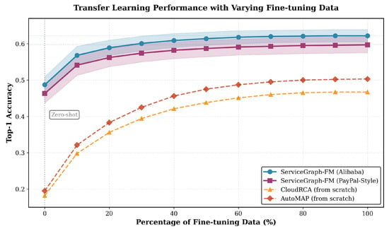
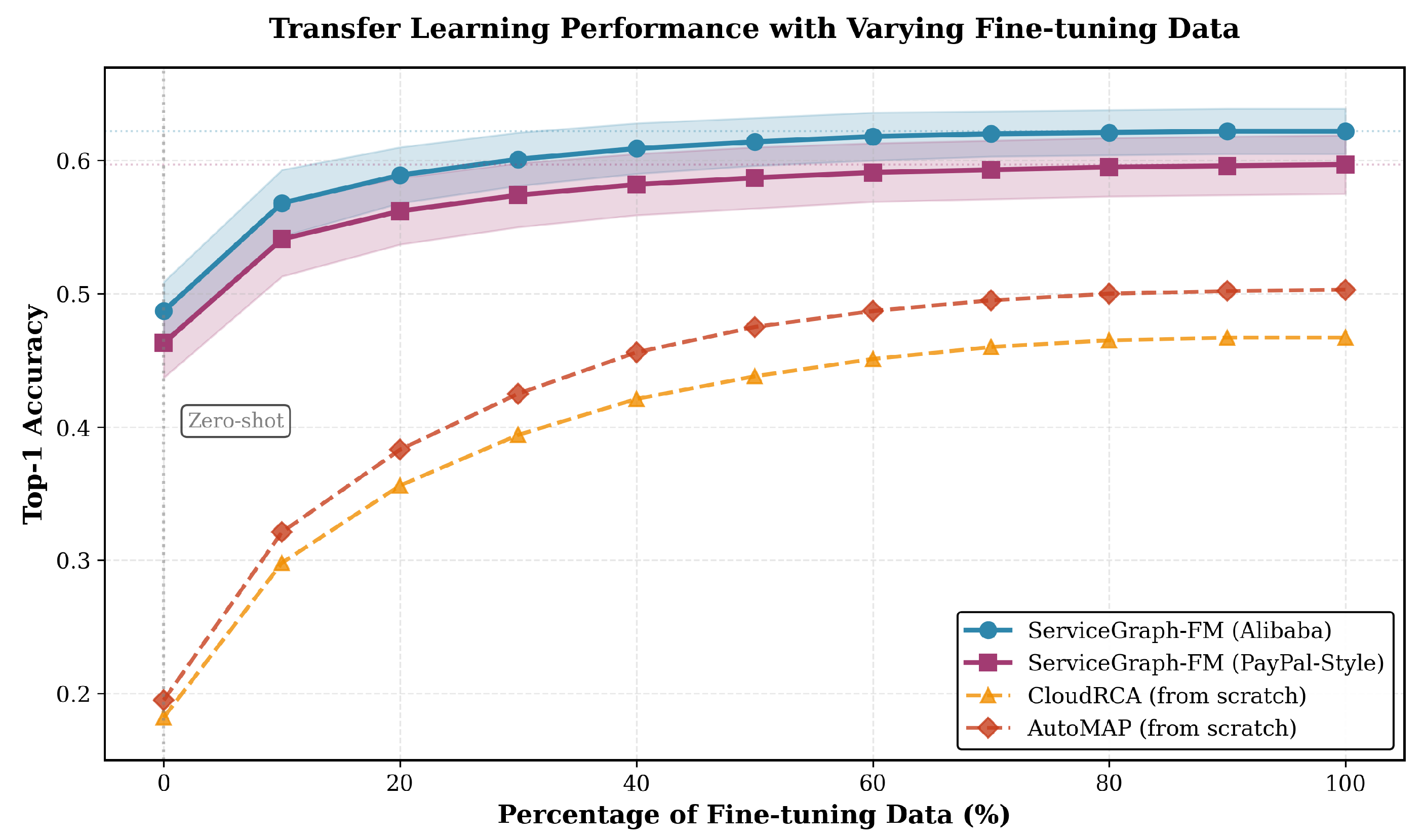
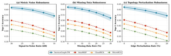
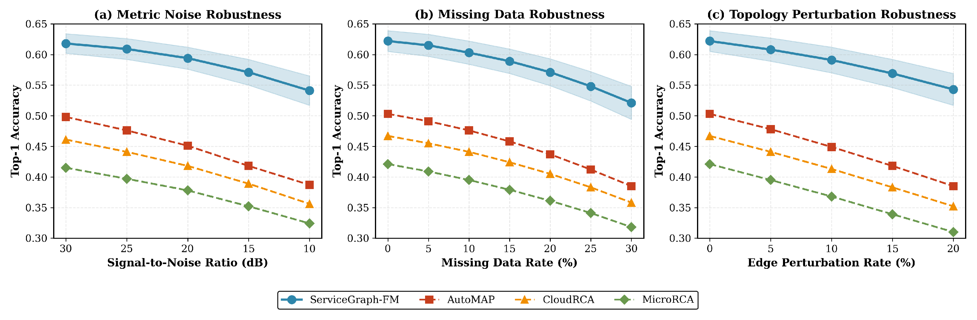
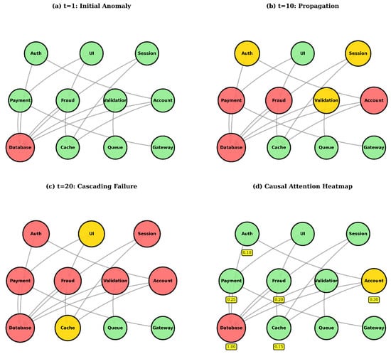
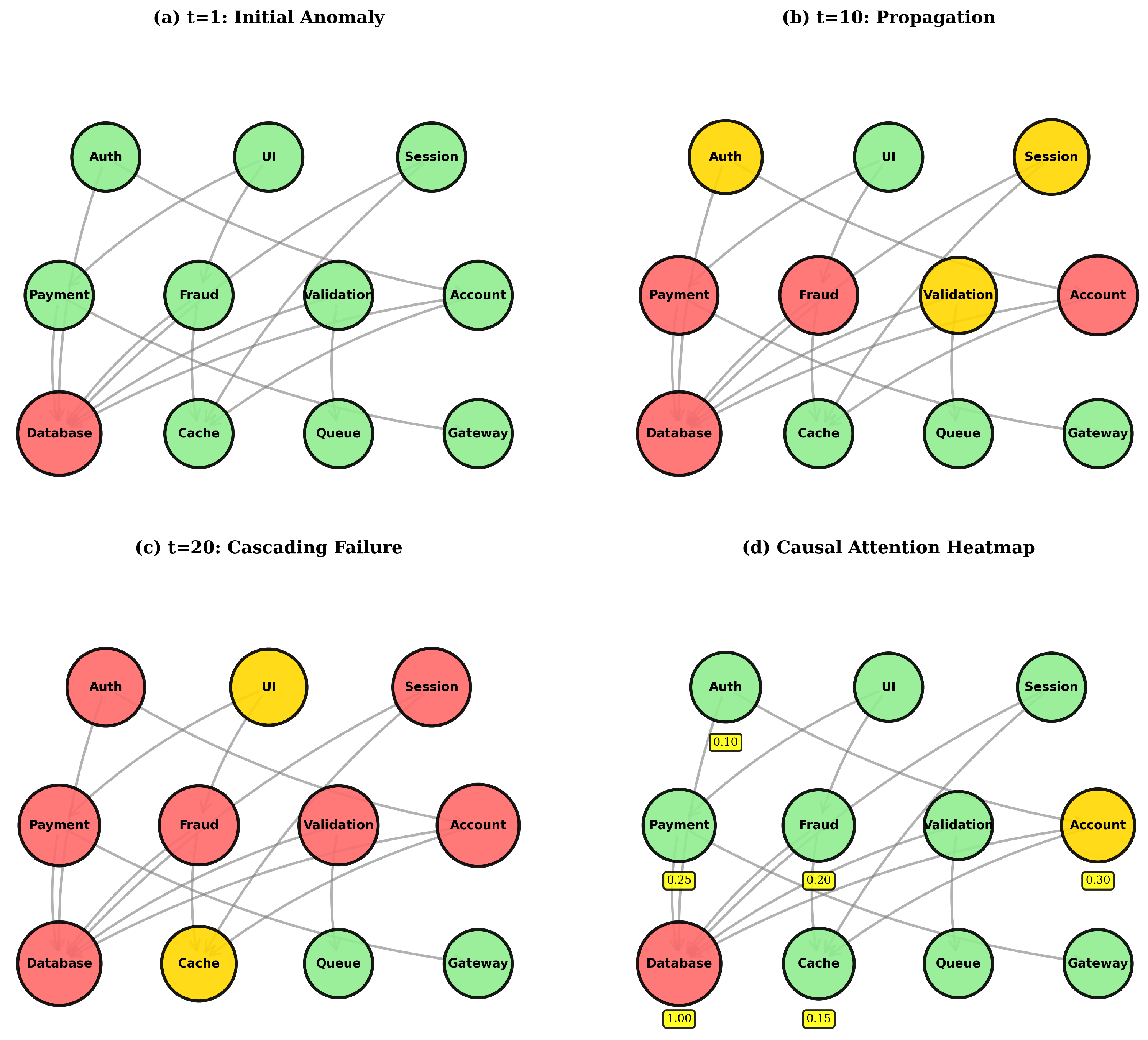

Disclaimer/Publisher’s Note: The statements, opinions and data contained in all publications are solely those of the individual author(s) and contributor(s) and not of MDPI and/or the editor(s). MDPI and/or the editor(s) disclaim responsibility for any injury to people or property resulting from any ideas, methods, instructions or products referred to in the content. |
© 2026 by the authors. Licensee MDPI, Basel, Switzerland. This article is an open access article distributed under the terms and conditions of the Creative Commons Attribution (CC BY) license.