Recovering the Fractional Order and an Initial Value Simultaneously in a Time-Fractional Diffusion-Wave Equation

Abstract

For a one-dimensional time-fractional diffusion-wave equation, we investigate joint recovery of its fractional order and the initial velocity from measurements taken at one interior point. Uniqueness is proved through analytic continuation, Laplace transforms, an integral mean value theorem, and Mittag-Leffler function properties. The ill-posed reconstruction is regularized in a Bayesian setting using the iterative regularizing ensemble Kalman method. The posterior measure is shown to exist and to depend stably on the data; its numerical approximation converges under an assumed error bound for the forward solver. The resulting method is assessed in three numerical tests, which illustrate its effectiveness as well as its stability.

1. Introduction

In recent decades, classical diffusion phenomena have been predominantly modeled by integer-order diffusion equations. Nevertheless, a wide range of empirical observations, notably fluid dynamics within porous media and the transport of macromolecules through biological systems [1,2,3], have revealed that these diffusion behaviors cannot be accurately captured by classical models. Such phenomena are referred to as anomalous diffusion. Fractional models account for hereditary and memory effects through their operators, making them better suited to describing anomalous diffusion. The temporal derivative can be generalized to a fractional order: $\alpha \in (0,1)$ leads to the time-fractional diffusion equation, whereas $\alpha \in (1,2)$ gives its diffusion-wave counterpart. Fractional diffusion models have been used to describe heterogeneous aquifers, wave propagation in viscoelastic materials, and heat conduction in fractal media [4,5,6,7]. These applications have motivated extensive research in recent years.

We investigate the following one-dimensional time-fractional diffusion-wave problem, where $l>0$ is the spatial length and $T>0$ is the final time:

$$\left\{\begin{array}{cc}\hfill {\partial }_{0+}^{\alpha }u\left(x,t\right)& =\Delta u\left(x,t\right)+F\left(x,t\right),x\in (0,l),t\in (0,T],1<\alpha <2,\hfill \\ \hfill u\left(0,t\right)& =u\left(l,t\right)=0,t\in (0,T],\hfill \\ \hfill u\left(x,0\right)& =a\left(x\right),x\in [0,l],\hfill \\ \hfill u_t\left(x,0\right)& =b\left(x\right),x\in [0,l].\hfill \end{array}\right.$$

(1)

Here ${\partial }_{0+}^{\alpha }$ denotes the left-sided Caputo fractional derivative of order $\alpha$ [8,9], defined by

$${\partial }_{0+}^{\alpha }u\left(x,t\right)={\displaystyle \frac{1}{\mathsf{\Gamma }\left(2-\alpha \right)}}{\int }_0^t{\displaystyle \frac{{\partial }^{2}u\left(x,\tau \right)}{\partial {\tau }^2}}{\displaystyle \frac{d\tau }{{\left(t-\tau \right)}^{\alpha -1}}},t\in (0,T],$$

where $\mathsf{\Gamma }(·)$ denotes the standard Gamma function.

Once the initial displacement $a\left(x\right)$, the initial velocity $b\left(x\right)$, the source $F(x,t)$, and the order $\alpha$ are prescribed, Equation (1) defines the direct problem. Its well-posedness and numerical approximation have been studied extensively [8,10,11,12,13,14]. For related variable-order fractional partial differential equations, Sabermahani et al. [15] developed a numerical method based on general Lagrange scaling functions.

Inverse problems for these models seek unknown initial states, coefficients, or fractional orders from additional measurements. In the diffusion-wave regime $1<\alpha <2$, the fractional order $\alpha$ characterizes the temporal memory of the model, while the initial velocity $b\left(x\right)$ describes the initial rate of change of the state. When neither quantity is known accurately, their joint recovery enables simultaneous identification of the memory parameter and the initial excitation. Here we jointly identify the fractional order $\alpha$ and the initial velocity $b\left(x\right)$ from the single interior trace

$$u\left(x_0,t\right)=g\left(t\right),t\in (0,T].$$

(2)

Realistically, one only acquires perturbed measurements $g^{\delta }$ rather than the true g. We presume the condition

$${\parallel g^{\delta }-g\parallel }_{L^2\left(0,T\right)}\le \delta ,$$

(3)

with $\delta >0$ specifying the noise level.

Interest in inverse recovery for these time-fractional diffusion-wave models has grown in recent years. Guided by the varied forms of acquired observational data, a broad spectrum of theoretical and numerical frameworks has been proposed for recovering the fractional order alongside unknown source terms, initial data, and coefficients. Xian and Wei [16] proved uniqueness for the time-fractional diffusion-wave equation and recovered its initial condition from final-time data. Their numerical procedure combines Tikhonov regularization with conjugate gradient iteration. For time-fractional diffusion-wave equations with a zero source term, Yamamoto [17] established that the fractional order and the initial data can be uniquely determined simultaneously from several types of measurements. The argument uses eigenfunction expansions and the asymptotic behavior of Mittag-Leffler functions. Wei and Deng [18] treated the joint identification of a time-varying potential coefficient and the fractional order in a time-fractional diffusion-wave model. They proved uniqueness and used a linearized iteration combined with Tikhonov-type regularization. Yang et al. [19] studied source identification for a Caputo–Hadamard type time-fractional diffusion-wave equation. They established conditional stability and developed fractional Tikhonov and fractional Landweber regularization methods, with error estimates under a priori and a posteriori parameter choice rules. Yan et al. [20] investigated the simultaneous recovery of a random source term and two initial values in a stochastic time-fractional diffusion-wave equation. They employed Tikhonov regularization and derived error estimates under a priori and a posteriori parameter choice rules. Wei et al. [21] incorporated an $H^1$-norm penalty into Tikhonov-type regularization for joint reconstruction of the spatially dependent source term and the fractional order. For their time-fractional diffusion-wave model, they analyzed uniqueness as well as convergence. Chang and Wei [22] considered the time-fractional convection-diffusion-wave equation and proved uniqueness for its inverse problem. Their reconstruction scheme couples Tikhonov-type regularization with Nesterov’s accelerated steepest descent method to recover the fractional order and the space-dependent source term together. Xian et al. [23] recovered a space-dependent potential coefficient from final-time measurements for a time-fractional diffusion-wave equation by a Banach space regularization scheme with a mixed $L^1$–$L^2$ penalty.

The iterative regularizing ensemble Kalman method (IREKM) has also been widely studied for inverse reconstruction. Zhang [24] developed a Bayesian IREKM procedure for a time-fractional diffusion-wave model, targeting simultaneous recovery of a time-varying source term and the fractional order. Uniqueness was also established for this recovery problem. For a one-dimensional time-fractional diffusion-wave model, Xian et al. [25] established uniqueness in simultaneous parameter recovery. Their Bayesian IREKM procedure reconstructed the fractional order jointly with two further unknowns, namely the initial velocity and the Neumann boundary data. Yan et al. [26] used Gel’fand-Levitan theory together with Laplace transforms to prove uniqueness for a one-dimensional time-fractional diffusion-wave model. They then applied IREKM to reconstruct the diffusion coefficient jointly with the fractional order. Here, this approach is used to infer the fractional order together with the initial velocity from one interior observation trace, while the source term and initial displacement remain prescribed.

Neural-network-based solvers have also been developed for related time-fractional diffusion equations. In particular, Shiri et al. [27] proposed an adaptive learning neural network method for the direct problem, employing an adaptive gradient-descent strategy to minimize the associated energy function. This provides a flexible alternative for forward approximation, whereas the present work uses the IREKM framework for noisy inverse identification of the fractional order and the initial velocity.

The main contributions of this work are as follows. We establish the unique determination of the fractional order and initial velocity from a single interior time trace, with a prescribed time-dependent source and initial displacement. The source contribution depends on the unknown fractional order, so the uniqueness result cannot be obtained by simply reducing the problem to the homogeneous case. Within a Bayesian framework, we establish posterior existence and stability with respect to the data, together with convergence of the approximate posterior under an assumed forward-solver error bound. We then apply IREKM for derivative-free joint reconstruction and assess its effectiveness and stability through numerical experiments, including a comparison with Tikhonov regularization.

Our identifiability proof for the unknown parameter pair uses Mittag-Leffler function properties, Laplace transforms, an integral mean value theorem, and analytic continuation. We then carry out the numerical reconstruction with IREKM in a Bayesian formulation.

The remaining sections proceed from analysis to numerical reconstruction. Section 2 collects the preliminary results used below. Section 3 proves uniqueness of the unknown parameter pair. Section 4 develops the Bayesian formulation and establishes posterior existence and data stability. It also proves convergence of the approximate posterior under a forward-solver error assumption. The section then describes IREKM for numerical reconstruction. Section 5 presents three one-dimensional computational examples to confirm the proposed algorithm’s performance and stability, followed by final remarks in Section 6.

2. Preliminaries

The definitions and several lemmas are presented in this section.

Definition 1

([28]). For parameters $\alpha >0$ and $\beta \in \mathbb{C}$, the Mittag-Leffler function is defined by

$$E_{\alpha ,\beta }\left(z\right)={\displaystyle \sum _{k=0}^{\infty }}{\displaystyle \frac{z^k}{\mathsf{\Gamma }(\alpha k+\beta )}},z\in \mathbb{C}.$$

(4)

Lemma 1

([9]). Fix $0<\alpha <2$ and $\beta \in \mathbb{R}$. For each $\mu \in \left({\displaystyle \frac{\pi \alpha }{2}},\min \left\{\pi ,\pi \alpha \right\}\right)$, the estimate below holds with a constant $C=C\left(\alpha ,\beta ,\mu \right)>0$:

$$\left|E_{\alpha ,\beta }\left(z\right)\right|\le {\displaystyle \frac{C}{1+\left|z\right|}},\mu \le \mid \mathit{arg}\left(z\right)\mid \le \pi .$$

(5)

Lemma 2

([28]). With $\alpha >0$ and $\beta >0$, the Laplace transform involving the Mittag-Leffler function can be evaluated as

$$\mathcal{L}\left\{t^{\beta -1}{E}_{\alpha ,\beta }\left(\pm \lambda t^{\alpha }\right)\right\}\left(s\right)={\displaystyle \frac{s^{\alpha -\beta }}{s^{\alpha }\mp \lambda }},\mathrm{Re}\left(s\right)>{\left|\lambda \right|}^{{\displaystyle \frac{1}{\alpha }}}.$$

(6)

Let ${\left\{{\lambda }_n,{\varphi }_n\left(x\right)\right\}}_{n=1}^{\infty }$ be the eigenpairs of the operator $-\Delta$ on $[0,l]$ with zero boundary values. They satisfy $-\Delta {\varphi }_n\left(x\right)={\lambda }_n{\varphi }_n\left(x\right)$ and ${\varphi }_n\left(0\right)={\varphi }_n\left(l\right)=0$. The explicit expressions are

$${\lambda }_n={\left({\displaystyle \frac{n\pi }{l}}\right)}^2,{\varphi }_n\left(x\right)=\sqrt{{\displaystyle \frac{2}{l}}}\sin \left({\displaystyle \frac{n\pi x}{l}}\right),n=1,2,\cdots .$$

The eigenvalues are ordered as $0<{\lambda }_1<{\lambda }_2<\cdots <{\lambda }_n<\cdots$, while the eigenfunctions ${\left\{{\varphi }_n\left(x\right)\right\}}_{n=1}^{\infty }$ constitute a complete orthonormal system in $L^2\left(0,l\right)$.

We use the Hilbert space $D\left({\left(-\Delta \right)}^{\gamma }\right)$, defined for $\gamma \ge 0$ by

$$D\left({\left(-\Delta \right)}^{\gamma }\right)=\left\{\psi \in L^2\left(0,l\right);{\displaystyle \sum _{n=1}^{\infty }}{\lambda }_n^{2\gamma }{\left|\left(\psi ,{\varphi }_n\right)\right|}^2<\infty \right\},$$

and the corresponding norm takes the form

$${\parallel \psi \parallel }_{D\left({\left(-\Delta \right)}^{\gamma }\right)}={\left({\displaystyle \sum _{n=1}^{\infty }}{\lambda }_n^{2\gamma }{\left|\left(\psi ,{\varphi }_n\right)\right|}^2\right)}^{{\displaystyle \frac{1}{2}}},$$

in which $(·,·)$ denotes the standard inner product in $L^2(0,l)$.

The space $C([0,T];L^2(0,l))$ consists of $L^2(0,l)$-valued functions that are continuous in time with respect to the norm of $L^2(0,l)$, equipped with the norm

$${\parallel u\parallel }_{C([0,T];L^2(0,l))}=\underset{t\in [0,T]}{\max }{\parallel u(·,t)\parallel }_{L^2(0,l)}.$$

The Bochner space $L^2(0,T;L^2(0,l))$ consists of equivalence classes of strongly measurable $L^2(0,l)$-valued functions satisfying

$${\parallel u\parallel }_{L^2(0,T;L^2(0,l))}={\left({\int }_0^T{\parallel u(·,t)\parallel }_{L^2(0,l)}^{2}dt\right)}^{1/2}<\infty .$$

Thus, the inner space $L^2(0,l)$ describes spatial square integrability, while the outer notation specifies continuity or square integrability in time.

Lemma 3

([8]). Under the assumptions $\alpha \in (1,2),a\left(x\right)\in L^2(0,l),b\left(x\right)\in L^2(0,l)$ and $F(x,t)\in L^2(0,T;L^2(0,l))$, problem (1) has exactly one weak solution $u\in C([0,T];L^2(0,l))$, represented by

$$\begin{array}{cc}\hfill u(x,t)=& {\displaystyle \sum _{n=1}^{\infty }}\left[(a,{\varphi }_n)E_{\alpha ,1}(-{\lambda }_n{t}^{\alpha })+(b,{\varphi }_n)t{E}_{\alpha ,2}(-{\lambda }_n{t}^{\alpha })\right]{\varphi }_n\left(x\right)\hfill \\ \hfill +& {\displaystyle \sum _{n=1}^{\infty }}\left({\int }_0^t(F(·,\tau ),{\varphi }_n){(t-\tau )}^{\alpha -1}{E}_{\alpha ,\alpha }(-{\lambda }_n{(t-\tau )}^{\alpha })d\tau \right){\varphi }_n\left(x\right).\hfill \end{array}$$

(7)

3. Uniqueness of the Inverse Problem

This paper investigates the simultaneous identification of the fractional order $\alpha$ and initial velocity $b\left(x\right)$ from a single interior trace for the 1D inhomogeneous diffusion-wave equation. While prior studies have addressed the homogeneous case under weaker $L^2$ regularity [17] or utilized dual endpoint traces to recover broader parameter sets [29], our setting uniquely incorporates a prescribed time-dependent source $F(x,t)$ and initial displacement $a\left(x\right)$. Since the source response depends on the unknown $\alpha$, simple subtraction is invalid. We overcome this via the non-degeneracy condition $F(x_0,0)+(\Delta a)\left(x_0\right)\ne 0$, which extracts $\alpha$ through short-time asymptotics, subsequently enabling the spectral recovery of $b\left(x\right)$. Consequently, the primary contribution of this paper lies in establishing the theoretical uniqueness for this prescribed-source setting, and providing numerical reconstruction results using the iterative regularizing ensemble Kalman method within a Bayesian framework.

We now state and prove the main theorem of this paper, followed by a comprehensive proof.

Theorem 1.

Let $\alpha ,\tilde{\alpha }\in (1,2),a\left(x\right)\in D\left({(-\Delta )}^{{\gamma }_1}\right),b\left(x\right),\tilde{b}\left(x\right)\in D\left({(-\Delta )}^{{\gamma }_2}\right),F\left(x,t\right)\in C(\left[0,T\right];$$D\left({(-\Delta )}^{{\gamma }_2}\right))$. Suppose $x_0\in (0,l)$ satisfies ${\displaystyle \frac{x_0}{l}}\notin \mathbb{Q}$, $F\left(x_0,0\right)+\left(\Delta a\right)\left(x_0\right)\ne 0$. Write $u\left(x,t\right)$ and $\tilde{u}\left(x,t\right)$ for the direct solutions of (1) corresponding, respectively, to $\left(\alpha ,b\left(x\right)\right)$ and $\left(\tilde{\alpha },\tilde{b}\left(x\right)\right)$. If

$$u\left(x_0,t\right)=\tilde{u}\left(x_0,t\right)=g\left(t\right),t\in \left(0,T\right],$$

this yields $\alpha =\tilde{\alpha },b\left(x\right)=\tilde{b}\left(x\right)$, in which ${\gamma }_1>{\displaystyle \frac{5}{4}},{\gamma }_2>{\displaystyle \frac{3}{4}}$.

Proof. 

Lemma 3 provides the series representation (7) of the weak solution. To verify that (7) converges uniformly on $[0,l]\times [0,T]$, we separate it into three terms:

$$\begin{array}{cc}\hfill u\left(x,t\right)& ={\displaystyle \sum _{n=1}^{\infty }}\left(a,{\varphi }_n\right)E_{\alpha ,1}\left(-{\lambda }_n{t}^{\alpha }\right){\varphi }_n\left(x\right)+{\displaystyle \sum _{n=1}^{\infty }}\left(b,{\varphi }_n\right)t{E}_{\alpha ,2}\left(-{\lambda }_n{t}^{\alpha }\right){\varphi }_n\left(x\right)\hfill \\ \hfill & +{\displaystyle \sum _{n=1}^{\infty }}{\int }_0^t\left(F\left(·,\tau \right),{\varphi }_n\right){\left(t-\tau \right)}^{\alpha -1}{E}_{\alpha ,\alpha }\left(-{\lambda }_n{\left(t-\tau \right)}^{\alpha }\right)d\tau {\varphi }_n\left(x\right)\hfill \\ \hfill & :=u_1(x,t)+u_2(x,t)+u_3(x,t).\hfill \end{array}$$

(8)

Combining the Liouville transform with Theorem 1.1.3 from [30] yields the following bound, where $C_{\varphi }$ denotes a constant:

$${\parallel {\varphi }_n\left(x\right)\parallel }_{C\left[0,l\right]}\le C_{\varphi }.$$

For $u_1(x,t)$, Lemma 1 gives the estimate

$$\begin{array}{cc}\hfill \left|u_1\left(x,t\right)\right|& =\left|{\displaystyle \sum _{n=1}^{\infty }}\left(a,{\varphi }_n\right)E_{\alpha ,1}\left(-{\lambda }_n{t}^{\alpha }\right){\varphi }_n\left(x\right)\right|\le {\displaystyle \sum _{n=1}^{\infty }}\left|\left(a,{\varphi }_n\right)E_{\alpha ,1}\left(-{\lambda }_n{t}^{\alpha }\right){\varphi }_n\left(x\right)\right|\hfill \\ \hfill & \le C_{\varphi }{\displaystyle \sum _{n=1}^{\infty }}\left|\left(a,{\varphi }_n\right)\right|{\displaystyle \frac{C}{1+{\lambda }_n{t}^{\alpha }}}\le C{C}_{\varphi }{\displaystyle \sum _{n=1}^{\infty }}\left|\left(a,{\varphi }_n\right)\right|\hfill \\ \hfill & =C{C}_{\varphi }{\displaystyle \sum _{n=1}^{\infty }}\left|\left(a,{\varphi }_n\right){\lambda }_n^{{\gamma }_1}\right|{\lambda }_n^{-{\gamma }_1}\le C{C}_{\varphi }{\left({\displaystyle \sum _{n=1}^{\infty }}{\left|\left(a,{\varphi }_n\right)\right|}^2{\lambda }_n^{2{\gamma }_1}\right)}^{{\displaystyle \frac{1}{2}}}{\left({\displaystyle \sum _{n=1}^{\infty }}{\lambda }_n^{-2{\gamma }_1}\right)}^{{\displaystyle \frac{1}{2}}}\hfill \\ \hfill & =C{C}_{\varphi }{\parallel a\parallel }_{D\left({\left(-\Delta \right)}^{{\gamma }_1}\right)}{\left({\displaystyle \sum _{n=1}^{\infty }}{\lambda }_n^{-2{\gamma }_1}\right)}^{{\displaystyle \frac{1}{2}}}.\hfill \end{array}$$

(9)

As ${\lambda }_n\backsim n^2$ and ${\gamma }_1>{\displaystyle \frac{5}{4}}$, it is evident that ${\sum }_{n=1}^{\infty }{\lambda }_n^{-2{\gamma }_1}<+\infty$. This entails that $u_1\left(x,t\right)$ converges uniformly on $\left[0,l\right]\times \left[0,T\right]$.

Analyzing $u_2(x,t)$, we have

$$\begin{array}{cc}\hfill \left|u_2\left(x,t\right)\right|& =\left|{\displaystyle \sum _{n=1}^{\infty }}\left(b,{\varphi }_n\right)t{E}_{\alpha ,2}\left(-{\lambda }_n{t}^{\alpha }\right){\varphi }_n\left(x\right)\right|\le {\displaystyle \sum _{n=1}^{\infty }}\left|\left(b,{\varphi }_n\right)t{E}_{\alpha ,2}\left(-{\lambda }_n{t}^{\alpha }\right){\varphi }_n\left(x\right)\right|\hfill \\ \hfill & \le C_{\varphi }{\displaystyle \sum _{n=1}^{\infty }}\left|\left(b,{\varphi }_n\right)\right|t{\displaystyle \frac{C}{1+{\lambda }_n{t}^{\alpha }}}\le C{C}_{\varphi }T{\displaystyle \sum _{n=1}^{\infty }}\left|\left(b,{\varphi }_n\right)\right|\hfill \\ \hfill & =C{C}_{\varphi }T{\displaystyle \sum _{n=1}^{\infty }}\left|\left(b,{\varphi }_n\right){\lambda }_n^{{\gamma }_2}\right|{\lambda }_n^{-{\gamma }_2}\le C{C}_{\varphi }T{\left({\displaystyle \sum _{n=1}^{\infty }}{\left|\left(b,{\varphi }_n\right)\right|}^2{\lambda }_n^{2{\gamma }_2}\right)}^{{\displaystyle \frac{1}{2}}}{\left({\displaystyle \sum _{n=1}^{\infty }}{\lambda }_n^{-2{\gamma }_2}\right)}^{{\displaystyle \frac{1}{2}}}\hfill \\ \hfill & =C{C}_{\varphi }T{\parallel b\parallel }_{D\left({\left(-\Delta \right)}^{{\gamma }_2}\right)}{\left({\displaystyle \sum _{n=1}^{\infty }}{\lambda }_n^{-2{\gamma }_2}\right)}^{{\displaystyle \frac{1}{2}}}.\hfill \end{array}$$

(10)

As ${\lambda }_n\backsim n^2$ and ${\gamma }_2>{\displaystyle \frac{3}{4}}$, we can show directly that ${\sum }_{n=1}^{\infty }{\lambda }_n^{-2{\gamma }_2}<+\infty$. This implies that $u_2\left(x,t\right)$ converges uniformly on $\left[0,l\right]\times \left[0,T\right]$.

Analyzing $u_3(x,t)$, we conclude that

$$\begin{array}{cc}\hfill \left|u_3\left(x,t\right)\right|& =\left|{\displaystyle \sum _{n=1}^{\infty }}{\int }_0^t\left(F\left(·,\tau \right),{\varphi }_n\right){\left(t-\tau \right)}^{\alpha -1}{E}_{\alpha ,\alpha }\left(-{\lambda }_n{\left(t-\tau \right)}^{\alpha }\right)d\tau {\varphi }_n\left(x\right)\right|\hfill \\ \hfill & \le {\displaystyle \sum _{n=1}^{\infty }}\left|{\int }_0^t\left(F\left(·,\tau \right),{\varphi }_n\right){\left(t-\tau \right)}^{\alpha -1}{E}_{\alpha ,\alpha }\left(-{\lambda }_n{\left(t-\tau \right)}^{\alpha }\right)d\tau {\varphi }_n\left(x\right)\right|\hfill \\ \hfill & \le C{C}_{\varphi }{\displaystyle \sum _{n=1}^{\infty }}{\int }_0^t\left|\left(F\left(·,\tau \right),{\varphi }_n\right)\right|{\left(t-\tau \right)}^{\alpha -1}d\tau \hfill \\ \hfill & =C{C}_{\varphi }{\int }_0^{\mathrm{t}}{\left(t-\tau \right)}^{\alpha -1}\left({\displaystyle \sum _{n=1}^{\infty }}\left|\left(F\left(·,\tau \right),{\varphi }_n\right)\right|\right)d\tau \hfill \\ \hfill & =C{C}_{\varphi }{\int }_0^{\mathrm{t}}{\left(t-\tau \right)}^{\alpha -1}\left({\displaystyle \sum _{n=1}^{\infty }}\left(\left|\left(F\left(·,\tau \right),{\varphi }_n\right)\right|{\lambda }_n^{{\gamma }_2}\right){\lambda }_n^{-{\gamma }_2}\right)d\tau \hfill \\ \hfill & \le C{C}_{\varphi }{\int }_0^{\mathrm{t}}{\left(t-\tau \right)}^{\alpha -1}{\left({\displaystyle \sum _{n=1}^{\infty }}{\left|\left(F\left(·,\tau \right),{\varphi }_n\right)\right|}^2{\lambda }_n^{2{\gamma }_2}\right)}^{{\displaystyle \frac{1}{2}}}{\left({\displaystyle \sum _{n=1}^{\infty }}{\lambda }_n^{-2{\gamma }_2}\right)}^{{\displaystyle \frac{1}{2}}}d\tau \hfill \\ \hfill & \le C{C}_{\varphi }{\int }_0^{\mathrm{t}}{\left(t-\tau \right)}^{\alpha -1}{\parallel F\parallel }_{C\left(\left[0,T\right];D\left({\left(-\Delta \right)}^{{\gamma }_2}\right)\right)}{\left({\displaystyle \sum _{n=1}^{\infty }}{\lambda }_n^{-2{\gamma }_2}\right)}^{{\displaystyle \frac{1}{2}}}d\tau \hfill \\ \hfill & =C{C}_{\varphi }{\parallel F\parallel }_{C\left(\left[0,T\right];D\left({\left(-\Delta \right)}^{{\gamma }_2}\right)\right)}{\left({\displaystyle \sum _{n=1}^{\infty }}{\lambda }_n^{-2{\gamma }_2}\right)}^{{\displaystyle \frac{1}{2}}}{\int }_0^t{\left(t-\tau \right)}^{\alpha -1}d\tau \hfill \\ \hfill & =C{C}_{\varphi }{\parallel F\parallel }_{C\left(\left[0,T\right];D\left({\left(-\Delta \right)}^{{\gamma }_2}\right)\right)}{\left({\displaystyle \sum _{n=1}^{\infty }}{\lambda }_n^{-2{\gamma }_2}\right)}^{{\displaystyle \frac{1}{2}}}{\displaystyle \frac{t^{\alpha }}{\alpha }}\hfill \\ \hfill & \le C{C}_{\varphi }{\displaystyle \frac{T^{\alpha }}{\alpha }}{\parallel F\parallel }_{C\left(\left[0,T\right];D\left({\left(-\Delta \right)}^{{\gamma }_2}\right)\right)}{\left({\displaystyle \sum _{n=1}^{\infty }}{\lambda }_n^{-2{\gamma }_2}\right)}^{{\displaystyle \frac{1}{2}}}.\hfill \end{array}$$

(11)

The relations ${\lambda }_n\backsim n^2$ and ${\gamma }_2>{\displaystyle \frac{3}{4}}$ imply ${\sum }_{n=1}^{\infty }{\lambda }_n^{-2{\gamma }_2}<+\infty$. Consequently, the series for $u_3\left(x,t\right)$ is uniformly convergent over $\left[0,l\right]\times \left[0,T\right]$.

In summary, we obtain $u\left(x,t\right)\in C\left(\left[0,l\right]\times \left[0,T\right]\right)$. Next, substituting $x_0$ into the analytical solution yields

$$\begin{array}{cc}\hfill u\left(x_0,t\right)=& {\displaystyle \sum _{n=1}^{\infty }}\left(a,{\varphi }_n\right)E_{\alpha ,1}\left(-{\lambda }_n{t}^{\alpha }\right){\varphi }_n\left(x_0\right)+{\displaystyle \sum _{n=1}^{\infty }}\left(b,{\varphi }_n\right)t{E}_{\alpha ,2}\left(-{\lambda }_n{t}^{\alpha }\right){\varphi }_n\left(x_0\right)\hfill \\ \hfill +& {\displaystyle \sum _{n=1}^{\infty }}{\int }_0^t\left(F\left(·,\tau \right),{\varphi }_n\right){\left(t-\tau \right)}^{\alpha -1}{E}_{\alpha ,\alpha }\left(-{\lambda }_n{\left(t-\tau \right)}^{\alpha }\right)d\tau {\varphi }_n\left(x_0\right).\hfill \end{array}$$

(12)

Based on $E_{\alpha ,\beta }\left(-z\right)={\displaystyle \frac{1}{\Gamma \left(\beta \right)}}-z{E}_{\alpha ,\alpha +\beta }\left(-z\right)$, this yields

$$\begin{array}{cc}\hfill u\left(x_0,t\right)& ={\displaystyle \sum _{n=1}^{\infty }}\left(a,{\varphi }_n\right){\varphi }_n\left(x_0\right)-t^{\alpha }{\displaystyle \sum _{n=1}^{\infty }}\left(a,{\varphi }_n\right){\lambda }_n{E}_{\alpha ,\alpha +1}\left(-{\lambda }_n{t}^{\alpha }\right){\varphi }_n\left(x_0\right)\hfill \\ \hfill & + t{\displaystyle \sum _{n=1}^{\infty }}\left(b,{\varphi }_n\right){\varphi }_n\left(x_0\right)-t^{\alpha +1}{\displaystyle \sum _{n=1}^{\infty }}\left(b,{\varphi }_n\right){\lambda }_n{E}_{\alpha ,\alpha +2}\left(-{\lambda }_n{t}^{\alpha }\right){\varphi }_n\left(x_0\right)\hfill \\ \hfill & + t^{\alpha }{\displaystyle \sum _{n=1}^{\infty }}\left[{\int }_0^t\left(F\left(·,\tau \right),{\varphi }_n\right){\displaystyle \frac{{\left(t-\tau \right)}^{\alpha -1}}{t^{\alpha }\Gamma \left(\alpha \right)}}d\tau \right]{\varphi }_n\left(x_0\right)\hfill \\ \hfill & -{\displaystyle \sum _{n=1}^{\infty }}\left[{\int }_0^t\left(F\left(·,\tau \right),{\varphi }_n\right){\lambda }_n{\left(t-\tau \right)}^{2\alpha -1}{E}_{\alpha ,2\alpha }\left(-{\lambda }_n{\left(t-\tau \right)}^{\alpha }\right)d\tau \right]{\varphi }_n\left(x_0\right)\hfill \\ \hfill & :=a\left(x_0\right)-t^{\alpha }{I}_{12}\left(t\right)+b\left(x_0\right)t-t^{\alpha +1}{I}_{22}\left(t\right)+t^{\alpha }{I}_{31}\left(t\right)-I_{32}\left(t\right),\hfill \end{array}$$

(13)

where

$$I_{12}\left(t\right)={\displaystyle \sum _{n=1}^{\infty }}\left(a,{\varphi }_n\right){\lambda }_n{E}_{\alpha ,\alpha +1}\left(-{\lambda }_n{t}^{\alpha }\right){\varphi }_n\left(x_0\right),$$

$$I_{22}\left(t\right)={\displaystyle \sum _{n=1}^{\infty }}\left(b,{\varphi }_n\right){\lambda }_n{E}_{\alpha ,\alpha +2}\left(-{\lambda }_n{t}^{\alpha }\right){\varphi }_n\left(x_0\right),$$

$$I_{31}\left(t\right)={\displaystyle \sum _{n=1}^{\infty }}\left[{\int }_0^t\left(F\left(·,\tau \right),{\varphi }_n\right){\displaystyle \frac{{\left(t-\tau \right)}^{\alpha -1}}{t^{\alpha }\Gamma \left(\alpha \right)}}d\tau \right]{\varphi }_n\left(x_0\right),$$

$$I_{32}\left(t\right)={\displaystyle \sum _{n=1}^{\infty }}\left[{\int }_0^t\left(F\left(·,\tau \right),{\varphi }_n\right){\lambda }_n{\left(t-\tau \right)}^{2\alpha -1}{E}_{\alpha ,2\alpha }\left(-{\lambda }_n{\left(t-\tau \right)}^{\alpha }\right)d\tau \right]{\varphi }_n\left(x_0\right).$$

Analyzing $I_{12}\left(t\right)$, we obtain

$$\begin{array}{cc}\hfill \left|I_{12}\left(t\right)\right|& =\left|{\displaystyle \sum _{n=1}^{\infty }}\left(a,{\varphi }_n\right){\lambda }_n{E}_{\alpha ,\alpha +1}\left(-{\lambda }_n{t}^{\alpha }\right){\varphi }_n\left(x_0\right)\right|\le {\displaystyle \sum _{n=1}^{\infty }}\left|\left(a,{\varphi }_n\right){\lambda }_n{E}_{\alpha ,\alpha +1}\left(-{\lambda }_n{t}^{\alpha }\right){\varphi }_n\left(x_0\right)\right|\hfill \\ \hfill & \le C_{\varphi }{\displaystyle \sum _{n=1}^{\infty }}\left|\left(a,{\varphi }_n\right)\right|{\displaystyle \frac{C{\lambda }_n}{1+{\lambda }_n{t}^{\alpha }}}\le C{C}_{\varphi }{\displaystyle \sum _{n=1}^{\infty }}\left|\left(a,{\varphi }_n\right)\right|{\lambda }_n=C{C}_{\varphi }{\displaystyle \sum _{n=1}^{\infty }}\left(\left|\left(a,{\varphi }_n\right)\right|{\lambda }_n^{{\gamma }_1}\right){\lambda }_n^{1-{\gamma }_1}\hfill \\ \hfill & \le C{C}_{\varphi }{\left({\displaystyle \sum _{n=1}^{\infty }}{\left|\left(a,{\varphi }_n\right)\right|}^2{\lambda }_n^{2{\gamma }_1}\right)}^{{\displaystyle \frac{1}{2}}}{\left({\displaystyle \sum _{n=1}^{\infty }}{\lambda }_n^{2\left(1-{\gamma }_1\right)}\right)}^{{\displaystyle \frac{1}{2}}}\hfill \\ \hfill & =C{C}_{\varphi }{\parallel a\parallel }_{D\left({\left(-\Delta \right)}^{{\gamma }_1}\right)}{\left({\displaystyle \sum _{n=1}^{\infty }}{\lambda }_n^{2\left(1-{\gamma }_1\right)}\right)}^{{\displaystyle \frac{1}{2}}}.\hfill \end{array}$$

The eigenvalue growth ${\lambda }_n\backsim n^2$, together with ${\gamma }_1>{\displaystyle \frac{5}{4}}$, yields ${\sum }_{n=1}^{\infty }{\lambda }_n^{2\left(1-{\gamma }_1\right)}<+\infty$. The series for $I_{12}\left(t\right)$ therefore converges uniformly throughout $\left[0,T\right]$. It follows that

$$\begin{array}{cc}\hfill \underset{t\to 0^{+}}{\lim }{I}_{12}\left(t\right)& =\underset{t\to 0^{+}}{\lim }{\displaystyle \sum _{n=1}^{\infty }}\left(a,{\varphi }_n\right){\lambda }_n{E}_{\alpha ,\alpha +1}\left(-{\lambda }_n{t}^{\alpha }\right){\varphi }_n\left(x_0\right)={\displaystyle \sum _{n=1}^{\infty }}\left(a,{\varphi }_n\right){\lambda }_n{\varphi }_n\left(x_0\right)E_{\alpha ,\alpha +1}\left(0\right)\hfill \\ \hfill & ={\displaystyle \sum _{n=1}^{\infty }}\left(a,{\varphi }_n\right){\lambda }_n{\varphi }_n\left(x_0\right){\displaystyle \frac{1}{\mathsf{\Gamma }\left(\alpha +1\right)}}={\displaystyle \frac{\left(\left(-\Delta \right)a\right)\left(x_0\right)}{\mathsf{\Gamma }\left(\alpha +1\right)}}.\hfill \end{array}$$

For $I_{22}\left(t\right)$, we have

$$\begin{array}{cc}\hfill \left|I_{22}\left(t\right)\right|& =\left|{\displaystyle \sum _{n=1}^{\infty }}\left(b,{\varphi }_n\right){\lambda }_n{E}_{\alpha ,\alpha +2}\left(-{\lambda }_n{t}^{\alpha }\right){\varphi }_n\left(x_0\right)\right|\le {\displaystyle \sum _{n=1}^{\infty }}\left|\left(b,{\varphi }_n\right){\lambda }_n{E}_{\alpha ,\alpha +2}\left(-{\lambda }_n{t}^{\alpha }\right){\varphi }_n\left(x_0\right)\right|\hfill \\ \hfill & \le C_{\varphi }{\displaystyle \sum _{n=1}^{\infty }}\left|\left(b,{\varphi }_n\right){\lambda }_n{E}_{\alpha ,\alpha +2}\left(-{\lambda }_n{t}^{\alpha }\right)\right|\le C{C}_{\varphi }{\displaystyle \sum _{n=1}^{\infty }}\left|\left(b,{\varphi }_n\right)\right|{\lambda }_n{\left({\lambda }_n{t}^{\alpha }\right)}^{-{\displaystyle \frac{1}{2}}}\hfill \\ \hfill & \le C{C}_{\varphi }{t}^{-{\displaystyle \frac{\alpha }{2}}}{\displaystyle \sum _{n=1}^{\infty }}\left|\left(b,{\varphi }_n\right)\right|{\lambda }_n^{{\displaystyle \frac{1}{2}}}=C{C}_{\varphi }{t}^{-{\displaystyle \frac{\alpha }{2}}}{\displaystyle \sum _{n=1}^{\infty }}\left(\left|\left(b,{\varphi }_n\right)\right|{\lambda }_n^{{\gamma }_2}\right){\lambda }_n^{{\displaystyle \frac{1}{2}}-{\gamma }_2}\hfill \\ \hfill & \le C{C}_{\varphi }{t}^{-{\displaystyle \frac{\alpha }{2}}}{\parallel b\parallel }_{D\left({\left(-\Delta \right)}^{{\gamma }_2}\right)}{\left({\displaystyle \sum _{n=1}^{\infty }}{\lambda }_n^{1-2{\gamma }_2}\right)}^{{\displaystyle \frac{1}{2}}}.\hfill \end{array}$$

(14)

The growth law ${\lambda }_n\backsim n^2$ and the assumption ${\gamma }_2>{\displaystyle \frac{3}{4}}$ ensure ${\sum }_{n=1}^{\infty }{\lambda }_n^{1-2{\gamma }_2}<+\infty$. Uniform convergence of the series for $I_{22}\left(t\right)$ holds on each interval $[\epsilon ,T]$ with $\epsilon \in (0,T)$. We also obtain

$$\left|I_{22}\left(t\right)\right|\le M_2{t}^{-{\displaystyle \frac{\alpha }{2}}}.$$

Since $1<\alpha <2$, this estimate also gives

$$|t{I}_{22}\left(t\right)|\le M_2{t}^{1-\alpha /2}⟶0,\mathrm{as}t\to 0^{+}.$$

For $I_{31}\left(t\right)$, the first mean value theorem for integrals selects an intermediate point ${\xi }_n\left(t\right)\in \left[0,t\right]$ such that

$$\begin{array}{cc}\hfill I_{31}\left(t\right)& ={\displaystyle \sum _{n=1}^{\infty }}\left[{\int }_0^t\left(F\left(·,\tau \right),{\varphi }_n\right){\displaystyle \frac{{\left(t-\tau \right)}^{\alpha -1}}{t^{\alpha }\Gamma \left(\alpha \right)}}d\tau \right]{\varphi }_n\left(x_0\right)\hfill \\ \hfill & ={\displaystyle \sum _{n=1}^{\infty }}\left(F\left(·,{\xi }_n\left(t\right)\right),{\varphi }_n\right){\displaystyle \frac{{\varphi }_n\left(x_0\right)}{t^{\alpha }\Gamma \left(\alpha \right)}}\left[{\int }_0^t{\left(t-\tau \right)}^{\alpha -1}d\tau \right]\hfill \\ \hfill & ={\displaystyle \sum _{n=1}^{\infty }}\left(F\left(·,{\xi }_n\left(t\right)\right),{\varphi }_n\right){\displaystyle \frac{{\varphi }_n\left(x_0\right)}{\alpha \Gamma \left(\alpha \right)}}={\displaystyle \sum _{n=1}^{\infty }}\left(F\left(·,{\xi }_n\left(t\right)\right),{\varphi }_n\right){\displaystyle \frac{{\varphi }_n\left(x_0\right)}{\Gamma \left(\alpha +1\right)}},\hfill \end{array}$$

(15)

since

$$\begin{array}{cc}\hfill \left|\left(F\left(·,{\xi }_n\left(t\right)\right),{\varphi }_n\right){\displaystyle \frac{{\varphi }_n\left(x_0\right)}{\Gamma \left(\alpha +1\right)}}\right|& \le {\displaystyle \frac{C_{\varphi }}{\Gamma \left(\alpha +1\right)}}\left|\left(F\left(·,{\xi }_n\left(t\right)\right),{\varphi }_n\right)\right|\hfill \\ & ={\displaystyle \frac{C_{\varphi }}{\Gamma \left(\alpha +1\right)}}\left|\left(F\left(·,{\xi }_n\left(t\right)\right),{\varphi }_n\right)\right|{\lambda }_n^{{\gamma }_2}·{\lambda }_n^{-{\gamma }_2},\hfill \end{array}$$

(16)

and

$$\begin{array}{cc}\hfill {\lambda }_n^{{\gamma }_2}\left|(F(·,{\xi }_n\left(t\right)),{\varphi }_n)\right|& {\le \parallel F(·,{\xi }_n\left(t\right))\parallel }_{D\left({(-\Delta )}^{{\gamma }_2}\right)}\hfill \\ \hfill & \le {\parallel F\parallel }_{C([0,T];D\left({(-\Delta )}^{{\gamma }_2}\right))}.\hfill \end{array}$$

(17)

And using ${\xi }_n\left(t\right)\in \left[0,t\right]\subset \left[0,T\right]$, we deduce

$$\underset{t\in (0,T]}{\sup }\left|\left(F\left(·,{\xi }_n\left(t\right)\right),{\varphi }_n\right){\displaystyle \frac{{\varphi }_n\left(x_0\right)}{\Gamma \left(\alpha +1\right)}}\right|\le {\displaystyle \frac{C_{\varphi }}{\Gamma \left(\alpha +1\right)}}{\parallel F\parallel }_{C\left(\left[0,T\right];D\left({\left(-\Delta \right)}^{{\gamma }_2}\right)\right)}{\lambda }_n^{-{\gamma }_2}.$$

As ${\lambda }_n\backsim n^2$ and ${\gamma }_2>{\displaystyle \frac{3}{4}}$, it is easy to prove ${\sum }_{n=1}^{\infty }{\lambda }_n^{-{\gamma }_2}<+\infty$. This shows that $I_{31}\left(t\right)$ converges uniformly on $(0,T]$.

For any fixed n, from the continuity of F and ${\xi }_n\left(t\right)\to 0$ as $t\to 0^{+}$, the termwise limit is obtained:

$$\underset{t\to 0^{+}}{\lim }\left(F\left(·,{\xi }_n\left(t\right)\right),{\varphi }_n\right)=\left(F\left(·,0\right),{\varphi }_n\right),$$

so that

$$\begin{array}{cc}\hfill \underset{t\to 0^{+}}{\lim }{I}_{31}\left(t\right)=& \underset{t\to 0^{+}}{\lim }{\displaystyle \sum _{n=1}^{\infty }}\left(F\left(·,{\xi }_n\left(t\right)\right),{\varphi }_n\right){\displaystyle \frac{{\varphi }_n\left(x_0\right)}{\Gamma \left(\alpha +1\right)}}\hfill \\ \hfill =& {\displaystyle \frac{1}{\Gamma \left(\alpha +1\right)}}{\displaystyle \sum _{n=1}^{\infty }}\left(F\left(·,0\right),{\varphi }_n\right){\varphi }_n\left(x_0\right)\hfill \\ \hfill =& {\displaystyle \frac{F\left(x_0,0\right)}{\Gamma \left(\alpha +1\right)}}.\hfill \end{array}$$

(18)

We next estimate $I_{32}\left(t\right)$. First, since $\left|E_{\alpha ,\beta }\left(-z\right)\right|\le {\displaystyle \frac{C}{1+\left|z\right|}}$, we have

$$z^{{\displaystyle \frac{1}{2}}}\left|E_{\alpha ,\beta }\left(-z\right)\right|\le z^{{\displaystyle \frac{1}{2}}}{\displaystyle \frac{C}{1+\left|z\right|}}=C{\displaystyle \frac{\sqrt{z}}{1+z}},z\ge 0.$$

Next, we analyze the function $f\left(z\right)={\displaystyle \frac{\sqrt{z}}{1+z}},z\ge 0$. When $z=1$, $f\left(z\right)$ attains its maximum value $f\left(1\right)={\displaystyle \frac{1}{2}}$; thus, we have

$$\left|E_{\alpha ,\beta }\left(-z\right)\right|\le {\displaystyle \frac{C}{2}}{z}^{-{\displaystyle \frac{1}{2}}},z>0,$$

so

$$\begin{array}{cc}\hfill \left|I_{32}\left(t\right)\right|& =\left|{\displaystyle \sum _{n=1}^{\infty }}\left[{\int }_0^t\left(F\left(·,\tau \right),{\varphi }_n\right){\lambda }_n{\left(t-\tau \right)}^{2\alpha -1}{E}_{\alpha ,2\alpha }\left(-{\lambda }_n{\left(t-\tau \right)}^{\alpha }\right)d\tau \right]{\varphi }_n\left(x_0\right)\right|\hfill \\ \hfill & \le {\displaystyle \sum _{n=1}^{\infty }}\left|\left[{\int }_0^t\left(F\left(·,\tau \right),{\varphi }_n\right){\lambda }_n{\left(t-\tau \right)}^{2\alpha -1}{E}_{\alpha ,2\alpha }\left(-{\lambda }_n{\left(t-\tau \right)}^{\alpha }\right)d\tau \right]{\varphi }_n\left(x_0\right)\right|\hfill \\ \hfill & \le C_{\varphi }{\displaystyle \sum _{n=1}^{\infty }}{\int }_0^t\left|\left(F\left(·,\tau \right),{\varphi }_n\right){\lambda }_n{\left(t-\tau \right)}^{2\alpha -1}{E}_{\alpha ,2\alpha }\left(-{\lambda }_n{\left(t-\tau \right)}^{\alpha }\right)\right|d\tau \hfill \\ \hfill & \le C{C}_{\varphi }{\displaystyle \sum _{n=1}^{\infty }}{\int }_0^t\left|\left(F\left(·,\tau \right),{\varphi }_n\right)\right|{\left(t-\tau \right)}^{2\alpha -1-{\displaystyle \frac{\alpha }{2}}}{\lambda }_n^{{\displaystyle \frac{1}{2}}}d\tau \hfill \\ \hfill & =C{C}_{\varphi }{\int }_0^t{\left(t-\tau \right)}^{{\displaystyle \frac{3\alpha }{2}}-1}\left({\displaystyle \sum _{n=1}^{\infty }}\left|\left(F\left(·,\tau \right),{\varphi }_n\right)\right|{\lambda }_n^{{\displaystyle \frac{1}{2}}}\right)d\tau .\hfill \end{array}$$

(19)

Holding $\tau$ fixed, we bound the inner series via the Cauchy–Schwarz inequality, which gives:

$$\begin{array}{cc}\hfill {\displaystyle \sum _{n=1}^{\infty }}\left|\left(F\left(·,\tau \right),{\varphi }_n\right)\right|{\lambda }_n^{{\displaystyle \frac{1}{2}}}& \le {\displaystyle \sum _{n=1}^{\infty }}\left(\left|\left(F\left(·,\tau \right),{\varphi }_n\right)\right|{\lambda }_n^{{\gamma }_2}\right){\lambda }_n^{{\displaystyle \frac{1}{2}}-{\gamma }_2}\hfill \\ \hfill & \le {\left[{\displaystyle \sum _{n=1}^{\infty }}\left({\left|\left(F\left(·,\tau \right),{\varphi }_n\right)\right|}^2{\lambda }_n^{2{\gamma }_2}\right)\right]}^{{\displaystyle \frac{1}{2}}}{\left({\displaystyle \sum _{n=1}^{\infty }}{\lambda }_n^{1-2{\gamma }_2}\right)}^{{\displaystyle \frac{1}{2}}}\hfill \\ \hfill & \le {\parallel F\left(·,\tau \right)\parallel }_{D\left({\left(-\Delta \right)}^{{\gamma }_2}\right)}{\left({\displaystyle \sum _{n=1}^{\infty }}{\lambda }_n^{1-2{\gamma }_2}\right)}^{{\displaystyle \frac{1}{2}}}\hfill \\ \hfill & \le \underset{\tau \in \left[0,T\right]}{\sup }{\parallel F\left(·,\tau \right)\parallel }_{D\left({\left(-\Delta \right)}^{{\gamma }_2}\right)}{\left({\displaystyle \sum _{n=1}^{\infty }}{\lambda }_n^{1-2{\gamma }_2}\right)}^{{\displaystyle \frac{1}{2}}}\hfill \\ \hfill & \le {\parallel F\parallel }_{C\left(\left[0,T\right];D\left({\left(-\Delta \right)}^{{\gamma }_2}\right)\right)}{\left({\displaystyle \sum _{n=1}^{\infty }}{\lambda }_n^{1-2{\gamma }_2}\right)}^{{\displaystyle \frac{1}{2}}}.\hfill \end{array}$$

(20)

As ${\lambda }_n\backsim n^2$ and ${\gamma }_2>{\displaystyle \frac{3}{4}}$, it is straightforward to prove ${\left({\sum }_{n=1}^{\infty }{\lambda }_n^{1-2{\gamma }_2}\right)}^{{\displaystyle \frac{1}{2}}}=M_1<+\infty$, so

$$\left|I_{32}\left(t\right)\right|\le C{C}_{\varphi }{\parallel F\parallel }_{C\left(\left[0,T\right];D\left({\left(-\Delta \right)}^{{\gamma }_2}\right)\right)}{M}_1{\int }_0^t{\left(t-\tau \right)}^{{\displaystyle \frac{3}{2}}\alpha -1}d\tau =O\left(t^{{\displaystyle \frac{3}{2}}\alpha }\right).$$

Using $u\left(x_0,t\right)=\tilde{u}\left(x_0,t\right)$, we cancel the common term $a\left(x_0\right)$ and obtain

$$\begin{array}{cc}\hfill & -t^{\alpha }{I}_{12}\left(t\right)+b\left(x_0\right)t-t^{\alpha +1}{I}_{22}\left(t\right)+t^{\alpha }{I}_{31}\left(t\right)-I_{32}\left(t\right)\hfill \\ \hfill =& -t^{\tilde{\alpha }}{\tilde{I}}_{12}\left(t\right)+\tilde{b}\left(x_0\right)t-t^{\tilde{\alpha }+1}{\tilde{I}}_{22}\left(t\right)+t^{\tilde{\alpha }}{\tilde{I}}_{31}\left(t\right)-{\tilde{I}}_{32}\left(t\right).\hfill \end{array}$$

(21)

To identify $\alpha$, divide Equation (21) by t and let $t\to 0^{+}$ to obtain

$$\underset{t\to 0^{+}}{\lim }\left[-t^{\alpha -1}{I}_{12}\left(t\right)+b\left(x_0\right)-t^{\alpha }{I}_{22}\left(t\right)+t^{\alpha -1}{I}_{31}\left(t\right)-t^{-1}{I}_{32}\left(t\right)\right]=b\left(x_0\right),$$

$$\underset{t\to 0^{+}}{\lim }\left[-t^{\tilde{\alpha }-1}{\tilde{I}}_{12}\left(t\right)+\tilde{b}\left(x_0\right)-t^{\tilde{\alpha }}{\tilde{I}}_{22}\left(t\right)+t^{\tilde{\alpha }-1}{\tilde{I}}_{31}\left(t\right)-t^{-1}{\tilde{I}}_{32}\left(t\right)\right]=\tilde{b}\left(x_0\right),$$

so $b\left(x_0\right)=\tilde{b}\left(x_0\right)$, and Equation (21) can be transformed into

$$-t^{\alpha }{I}_{12}\left(t\right)-t^{\alpha +1}{I}_{22}\left(t\right)+t^{\alpha }{I}_{31}\left(t\right)-I_{32}\left(t\right)=-t^{\tilde{\alpha }}{\tilde{I}}_{12}\left(t\right)-t^{\tilde{\alpha }+1}{\tilde{I}}_{22}\left(t\right)+t^{\tilde{\alpha }}{\tilde{I}}_{31}\left(t\right)-{\tilde{I}}_{32}\left(t\right).$$

(22)

To establish $\alpha =\tilde{\alpha }$, suppose instead that $1<\alpha <\tilde{\alpha }<2$. After division of (22) by $t^{\alpha }$, we obtain

$$-I_{12}\left(t\right)-t{I}_{22}\left(t\right)+I_{31}\left(t\right)-t^{-\alpha }{I}_{32}\left(t\right)=t^{\tilde{\alpha }-\alpha }\left(-{\tilde{I}}_{12}\left(t\right)-t{\tilde{I}}_{22}\left(t\right)+{\tilde{I}}_{31}\left(t\right)-t^{-\tilde{\alpha }}{\tilde{I}}_{32}\left(t\right)\right).$$

Taking $t\to 0^{+}$ yields

$$-{\displaystyle \frac{\left(\left(-\Delta \right)a\right)\left(x_0\right)}{\mathsf{\Gamma }\left(\alpha +1\right)}}+{\displaystyle \frac{F\left(x_0,0\right)}{\mathsf{\Gamma }\left(\alpha +1\right)}}={\displaystyle \frac{F\left(x_0,0\right)+\left(\Delta a\right)\left(x_0\right)}{\mathsf{\Gamma }\left(\alpha +1\right)}}=0,$$

then $F\left(x_0,0\right)+\left(\Delta a\right)\left(x_0\right)=0$.

The fact that $F\left(x_0,0\right)+\left(\Delta a\right)\left(x_0\right)\ne 0$ directly yields a contradiction. Analogous reasoning eliminates the possibility of $\alpha >\tilde{\alpha }$, which forces $\alpha =\tilde{\alpha }$.

We will prove $b=\tilde{b},x\in \left[0,l\right]$. When $\alpha =\tilde{\alpha }$, the residual equation degenerates to

$${\displaystyle \sum _{n=1}^{\infty }}\left(b-\tilde{b},{\varphi }_n\right){\varphi }_n\left(x_0\right)t{E}_{\alpha ,2}\left(-{\lambda }_n{t}^{\alpha }\right)=0,t\in \left(0,T\right].$$

(23)

We first prove ${\sum }_{n=1}^{\infty }\left(b-\tilde{b},{\varphi }_n\right){\varphi }_n\left(x_0\right)$ converges absolutely:

$$\begin{array}{cc}\hfill \left|{\displaystyle \sum _{n=1}^{\infty }}\left(b-\tilde{b},{\varphi }_n\right){\varphi }_n\left(x_0\right)\right|& \le {\displaystyle \sum _{n=1}^{\infty }}\left|\left(b-\tilde{b},{\varphi }_n\right){\varphi }_n\left(x_0\right)\right|\le C_{\varphi }{\displaystyle \sum _{n=1}^{\infty }}\left(\left|\left(b-\tilde{b},{\varphi }_n\right)\right|{\lambda }_n^{{\gamma }_2}\right){\lambda }_n^{-{\gamma }_2}\hfill \\ \hfill & \le C_{\varphi }{\left({\displaystyle \sum _{n=1}^{\infty }}\left({\left|\left(b-\tilde{b},{\varphi }_n\right)\right|}^2{\lambda }_n^{2{\gamma }_2}\right)\right)}^{{\displaystyle \frac{1}{2}}}{\left({\displaystyle \sum _{n=1}^{\infty }}{\lambda }_n^{-2{\gamma }_2}\right)}^{{\displaystyle \frac{1}{2}}}\hfill \\ \hfill & =C_{\varphi }{\parallel b-\tilde{b}\parallel }_{D\left({\left(-\Delta \right)}^{{\gamma }_2}\right)}{\left({\displaystyle \sum _{n=1}^{\infty }}{\lambda }_n^{-2{\gamma }_2}\right)}^{{\displaystyle \frac{1}{2}}}.\hfill \end{array}$$

(24)

As ${\lambda }_n\backsim n^2$ and ${\gamma }_2>{\displaystyle \frac{3}{4}}$, it is easy to prove ${\sum }_{n=1}^{\infty }\left|(b-\tilde{b},{\varphi }_n){\varphi }_n\left(x_0\right)\right|<\infty$.

Set $c_n=(b-\tilde{b},{\varphi }_n){\varphi }_n\left(x_0\right)$, so that ${\sum }_{n=1}^{\infty }\left|c_n\right|<\infty$. Choose

$$0<\vartheta <{\displaystyle \frac{\pi }{\alpha }}-{\displaystyle \frac{\pi }{2}},{\Sigma }_{\vartheta }=\{z\in \mathbb{C}\setminus \left\{0\right\}:|\arg z|<\vartheta \}.$$

Use the principal branch of $z^{\alpha }$ and choose $\mu$ such that $\pi \alpha /2<\mu <\pi -\alpha \vartheta$. For $z\in {\Sigma }_{\vartheta }$, we have $\left|\arg \right(-{\lambda }_n{z}^{\alpha }\left)\right|\ge \pi -\alpha \vartheta >\mu$. Lemma 1 therefore gives, for every compact set $K\subset {\Sigma }_{\vartheta }$,

$$|z{E}_{\alpha ,2}(-{\lambda }_n{z}^{\alpha })| \le {\displaystyle \frac{C\left|z\right|}{1+{\lambda }_n{\left|z\right|}^{\alpha }}}\le C_K,z\in K,$$

where $C_K$ is independent of n. The series ${\sum }_{n=1}^{\infty }{c}_{n}z{E}_{\alpha ,2}(-{\lambda }_n{z}^{\alpha })$ thus converges uniformly on every compact subset of ${\Sigma }_{\vartheta }$. Each summand is analytic there, so the sum is analytic in ${\Sigma }_{\vartheta }$.

As this analytic function evaluates to zero on the interval $(0,T]$, by the identity theorem, it follows that the function vanishes identically over the entire positive real axis. Thus, Equation (23) becomes

$${\displaystyle \sum _{n=1}^{\infty }}(b-\tilde{b},{\varphi }_n){\varphi }_n\left(x_0\right)t{E}_{\alpha ,2}(-{\lambda }_n{t}^{\alpha })=0,t>0.$$

(25)

We now take the Laplace transform of Equation (25). For each fixed n, the formula in Lemma 2 is initially valid only for $\mathrm{Re}\left(z\right)>{\lambda }_n^{1/\alpha }$. To extend this equality, we utilize analytic continuation. The uniform bound $|E_{\alpha ,2}(-x)|\le C$ for $x\ge 0$ gives the following absolute estimate for the integral at any complex point z with $\mathrm{Re}\left(z\right)>0$:

$${\int }_0^{+\infty }\left|e^{-zt}t{E}_{\alpha ,2}\left(-{\lambda }_n{t}^{\alpha }\right)\right|dt\le C{\int }_0^{+\infty }t{e}^{-\mathrm{Re}\left(z\right)t}dt={\displaystyle \frac{C}{{\left(\mathrm{Re}\left(z\right)\right)}^2}}<+\infty .$$

It follows that this integral constitutes an analytic function within the region $\mathrm{Re}\left(z\right)>0$. Meanwhile, for $1<\alpha <2$ and $\mathrm{Re}\left(z\right)>0$, the principal branch guarantees $\left|\arg \right(z^{\alpha }\left)\right|<\alpha \pi /2<\pi$, ensuring that $z^{\alpha }+{\lambda }_n\ne 0$. Thus, the function ${\displaystyle \frac{z^{\alpha -2}}{z^{\alpha }+{\lambda }_n}}$ is also analytic on $\mathrm{Re}\left(z\right)>0$. Invoking the identity theorem for analytic functions, the Laplace transform equality extends to $\mathrm{Re}\left(z\right)>0$.

For $\mathrm{Re}z>0$, the preceding bound and the absolute summability of $c_n$ yield

$${\displaystyle \sum _{n=1}^{\infty }}|c_n|{\int }_0^{\infty }{e}^{-\mathrm{Re}\left(z\right)t}t|E_{\alpha ,2}(-{\lambda }_n{t}^{\alpha })|dt\le {\displaystyle \frac{C}{{\left(\mathrm{Re}z\right)}^2}}{\displaystyle \sum _{n=1}^{\infty }}\left|c_n\right|<\infty .$$

Fubini’s theorem therefore permits interchange of the sum and integral. Multiplying Equation (25) by $e^{-zt}$ and integrating over $(0,\infty )$ gives

$$\begin{array}{cc}\hfill 0& ={\int }_0^{\infty }{e}^{-zt}{\displaystyle \sum _{n=1}^{\infty }}{c}_{n}t{E}_{\alpha ,2}(-{\lambda }_n{t}^{\alpha })dt\hfill \\ \hfill & ={\displaystyle \sum _{n=1}^{\infty }}{c}_n{\int }_0^{\infty }{e}^{-zt}t{E}_{\alpha ,2}(-{\lambda }_n{t}^{\alpha })dt\hfill \\ \hfill & =z^{\alpha -2}{\displaystyle \sum _{n=1}^{\infty }}{\displaystyle \frac{c_n}{z^{\alpha }+{\lambda }_n}},\mathrm{Re}z>0.\hfill \end{array}$$

(26)

Since $z^{\alpha -2}\ne 0,\mathrm{Re}\left(z\right)>0$, let $\eta =z^{\alpha }$, Equation (26) can be transformed into

$${\displaystyle \sum _{n=1}^{\infty }}{\displaystyle \frac{\left(b-\tilde{b},{\varphi }_n\right){\varphi }_n\left(x_0\right)}{\eta +{\lambda }_n}}=0.$$

(27)

Based on the absolute convergence verified previously, the Weierstrass theorem ensures that the series ${\sum }_{n=1}^{\infty }{\displaystyle \frac{(b-\tilde{b},{\varphi }_n){\varphi }_n\left(x_0\right)}{\eta +{\lambda }_n}}$ converges uniformly over any compact subset within $\mathbb{C}\setminus {\{-{\lambda }_n\}}_{n=1}^{\infty }$. Consequently, it defines an analytic function in $\mathbb{C}\setminus {\{-{\lambda }_n\}}_{n=1}^{\infty }$. Applying the identity theorem of analytic functions, the equality (27) holds throughout the connected domain $\mathbb{C}\setminus {\{-{\lambda }_n\}}_{n=1}^{\infty }$ via analytic extension.

For any fixed positive integer s, we choose a closed circular disk in the complex plane that encloses only the simple pole $-{\lambda }_s$ and excludes all other poles ${\{-{\lambda }_n\}}_{n\ne s}$. The contour integral of (27) around this disk, taken in the variable $\eta$, is evaluated by the residue theorem and gives

$$\left(b-\tilde{b},{\varphi }_s\right){\varphi }_s\left(x_0\right)=0.$$

Since $x_0/l\notin \mathbb{Q}$, it follows that ${\varphi }_s\left(x_0\right)\ne 0$. From this, we deduce that $\left(b-\tilde{b},{\varphi }_s\right)=0$. Given the completeness of the orthonormal basis within the real space $L^2(0,l)$, the vanishing of all Fourier coefficients implies that ${\parallel b\left(x\right)-\tilde{b}\left(x\right)\parallel }_{L^2(0,l)}=0$, thereby confirming that $b\left(x\right)=\tilde{b}\left(x\right)$. Thus, this concludes the proof of uniqueness regarding the inverse recovery of the multi-parameter pair $(\alpha ,b(x\left)\right)$.    □

4. Bayesian Formulation and Iterative Regularizing Ensemble Kalman Method

Section 3 establishes the theoretical uniqueness for the joint reconstruction involving the initial velocity b and the fractional order $\alpha$, which is deduced from exact interior measurements of $u(x_0,t)$ over a time interval. In practice, however, the observation is available only at finitely many time instants and is corrupted by measurement noise. In the present section, we begin by casting this inverse formulation within a Bayesian framework. We establish posterior existence and data stability, and analyze convergence of the approximate posterior under a forward-solver error assumption. Numerical recovery is then carried out with the iterative regularizing ensemble Kalman method (IREKM).

The Bayesian formulation and posterior analysis below follow the standard framework for statistical inverse problems described in [31,32,33].

To construct the Bayesian formulation, we first define the observation operator. Let

$$0<t_1<t_2<\cdots <t_M\le T$$

be the observation times and let $H=L^2(0,l)$. The known initial displacement a and the source term F are fixed throughout this section. For

$$\theta =(\alpha ,b)\in \mathcal{X}:=I_{\alpha }\times H,I_{\alpha }=[\underline{\alpha },\overline{\alpha }]⋐(1,2),$$

write $u(·,·;\theta )$ for the corresponding direct solution of (1). Its observed values define the operator

$$\mathcal{G}\left(\theta \right):={\left(u(x_0,t_1;\theta ),\cdots ,u(x_0,t_M;\theta )\right)}^{\mathsf{T}}\in {\mathbb{R}}^M.$$

(28)

The restriction $I_{\alpha }⋐(1,2)$ keeps the fractional order away from the endpoints and permits estimates that are uniform with respect to $\alpha$. Numerically, the interval may be chosen as $[1+{\epsilon }_{\alpha },2-{\epsilon }_{\alpha }]$ with a small ${\epsilon }_{\alpha }>0$.

The observation operator has the following properties.

Lemma 4.

Let a and F have the regularity specified in Section 3, and suppose that $t_1\ge t_{*}>0$. Then $\mathcal{G}:\mathcal{X}\to {\mathbb{R}}^M$ is continuous, and there is a constant $C_{\mathcal{G}}>0$ such that, for all $\alpha \in I_{\alpha }$ and $b,b_1,b_2\in H$,

$${\left|\mathcal{G}(\alpha ,b)\right|}_{{\mathbb{R}}^M}\le C_{\mathcal{G}}\left(1+{\Vert b\Vert }_H\right),$$

(29)

and

$$|\mathcal{G}(\alpha ,b_1)-\mathcal{G}(\alpha ,b_2){|}_{{\mathbb{R}}^M}\le C_{\mathcal{G}}{\Vert b_1-b_2\Vert }_H.$$

(30)

Proof. 

The contribution of b in (7) is

$$u_b(x_0,t;\alpha ,b)={\displaystyle \sum _{n=1}^{\infty }}{(b,{\varphi }_n)}_{H}t{E}_{\alpha ,2}(-{\lambda }_n{t}^{\alpha }){\varphi }_n\left(x_0\right).$$

(31)

Choose $\pi /2<\omega <\pi /\overline{\alpha }$. Let ${\mathcal{H}}_{\omega }$ consist of the rays $\arg \zeta =\pm \omega$, $\left|\zeta \right|\ge 1$, joined counterclockwise along the unit circle, oriented from the lower ray to the upper ray. The Hankel formula and analytic continuation give, with principal powers,

$$E_{\alpha ,\beta }(-r)={\displaystyle \frac{1}{2\pi i}}{\int }_{{\mathcal{H}}_{\omega }}{\displaystyle \frac{e^{\zeta }{\zeta }^{\alpha -\beta }}{{\zeta }^{\alpha }+r}}d\zeta ,\alpha \in I_{\alpha },\beta \in \{1,2,\alpha \},r\ge 0.$$

Since $\overline{\alpha }\omega <\pi$, the bound $|{\zeta }^{\alpha }+{r|\ge c(\left|\zeta \right|}^{\alpha }+r)\ge c(1+r)$ and exponential decay on the rays yield $|E_{\alpha ,\beta }(-r)|\le C/(1+r)$ uniformly in these parameters. For $t\in [t_{*},T]$, it follows that $|t{E}_{\alpha ,2}(-{\lambda }_n{t}^{\alpha })| \le C{\lambda }_n^{-1}$, and hence

$$|u_b(x_0,t;\alpha ,b){| \le C\parallel b\parallel }_H{\left({\displaystyle \sum _{n=1}^{\infty }}{\lambda }_n^{-2}\right)}^{1/2}\le C{\parallel b\parallel }_H.$$

Here we used the boundedness of ${\varphi }_n$ and ${\lambda }_n\asymp n^2$. Applying the same estimate to $b_1-b_2$ proves (30). The fixed a and F terms are bounded as in Section 3, giving (29); the uniform bounds and dominated convergence give continuity in $\alpha$, and thus continuity of $\mathcal{G}$.    □

We model the measured data through

$$d=\mathcal{G}\left(\theta \right)+\eta ,\eta \sim \mathcal{N}(0,\mathsf{\Gamma }),$$

(32)

where $\mathsf{\Gamma }\in {\mathbb{R}}^{M\times M}$ denotes the covariance matrix, assumed symmetric and positive definite. The noise $\eta$ is independent of $\theta$; for independent identically distributed noise components, one may choose $\mathsf{\Gamma }={\sigma }^2{I}_M$.

Let $A=-\Delta$ be the negative Dirichlet Laplacian on $(0,l)$. We prescribe the product prior

$${\mu }_0={\mu }_{\alpha }\otimes {\mu }_b,{\mu }_{\alpha }=\mathcal{U}\left(I_{\alpha }\right),{\mu }_b=\mathcal{N}(m_b,{\mathcal{C}}_b),$$

(33)

where $m_b\in H$ is the prescribed prior mean and

$${\mathcal{C}}_b=K{A}^{-s},K>0,s>{\displaystyle \frac{1}{2}}.$$

(34)

Here $\mathcal{U}\left(I_{\alpha }\right)$ denotes the uniform distribution on $I_{\alpha }$, while $\mathcal{N}(m_b,{\mathcal{C}}_b)$ denotes the Gaussian distribution with mean $m_b$ and covariance operator ${\mathcal{C}}_b=K{A}^{-s}$. The product prior assumes that $\alpha$ and b are independent. The operator A is discretized in the numerical implementation. Indeed, because ${\lambda }_n\asymp n^2$ in one space dimension,

$$\mathrm{Tr}\left({\mathcal{C}}_b\right)=K{\displaystyle \sum _{n=1}^{\infty }}{\lambda }_n^{-s}<\infty \mathrm{for}s>{\displaystyle \frac{1}{2}},$$

so that (34) defines a Gaussian Radon measure on H.

For $\theta \in \mathcal{X}$ and $d\in {\mathbb{R}}^M$, define the negative log-likelihood potential

$$\mathrm{\Phi }(\theta ;d):={\displaystyle \frac{1}{2}}{\parallel {\mathsf{\Gamma }}^{-1/2}\left(d-\mathcal{G}\left(\theta \right)\right)\parallel }_{{\mathbb{R}}^M}^2.$$

(35)

The likelihood is proportional to $\exp (-\mathrm{\Phi }(\theta ;d\left)\right)$.

We express the posterior relative to the prior as

$${\displaystyle \frac{\mathrm{d}{\mu }^d}{\mathrm{d}{\mu }_0}}\left(\theta \right)={\displaystyle \frac{1}{Z\left(d\right)}}\exp \left(-\mathrm{\Phi }(\theta ;d)\right),$$

(36)

where

$$Z\left(d\right):={\int }_{\mathcal{X}}\exp \left(-\mathrm{\Phi }(\theta ;d)\right){\mu }_0\left(\mathrm{d}\theta \right)$$

(37)

is the normalizing constant. Its positivity is established below.

Remark 1.

The condition $s>1/2$ is sufficient for defining the Gaussian prior on $H=L^2(0,l)$. If one additionally wants prior samples to belong almost surely to the stronger space $D\left(A^{\gamma }\right)$, it is sufficient to assume $m_b\in D\left(A^{\gamma }\right)$ and

$$s>2\gamma +{\displaystyle \frac{1}{2}}.$$

(38)

Indeed,

$$\mathbb{E}{\parallel A^{\gamma }(b-m_b)\parallel }_H^2=K{\displaystyle \sum _{n=1}^{\infty }}{\lambda }_n^{2\gamma -s}<\infty$$

under (38). In particular, compatibility with the regularity ${\gamma }_2>3/4$ in the uniqueness theorem is guaranteed by choosing $s>2{\gamma }_2+1/2$.

For two probability measures $\mu$ and $\nu$ that both admit densities relative to $\lambda$, we use the following definition of their Hellinger distance:

$$d_{Hell}^2(\mu ,\nu ):={\displaystyle \frac{1}{2}}{\int }_{\mathcal{X}}{\left(\sqrt{{\displaystyle \frac{\mathrm{d}\mu }{\mathrm{d}\lambda }}}-\sqrt{{\displaystyle \frac{\mathrm{d}\nu }{\mathrm{d}\lambda }}}\right)}^2\mathrm{d}\lambda .$$

(39)

Theorem 2

(Posterior existence and data stability). Under the preceding observation and prior assumptions, (36) defines a posterior probability measure ${\mu }^d$ for every $d\in {\mathbb{R}}^M$, with $0<Z\left(d\right)\le 1$. Moreover, for every $r>0$ there is $C_r>0$ such that, whenever $|d_1{|}_{{\mathbb{R}}^M},{\left|d_2\right|}_{{\mathbb{R}}^M}\le r$,

$$d_{Hell}({\mu }^{d_1},{\mu }^{d_2})\le C_r{\left|d_1-d_2\right|}_{{\mathbb{R}}^M}.$$

(40)

Proof. 

Lemma 4 makes $\mathrm{\Phi }(·;d)$ measurable and finite. Hence $0<e^{-\mathrm{\Phi }}\le 1$ gives $0<Z\left(d\right)\le 1$, and Bayes’ formula yields (36). Put $R\left(\theta \right)=1+{\parallel b\parallel }_H$, ${\mathrm{\Phi }}_i=\mathrm{\Phi }(\theta ;d_i)$ and $Z_i=Z\left(d_i\right)$. Choose a ball $B\subset H$ with ${\mu }_b\left(B\right)>0$. By (29), ${\mathrm{\Phi }}_i$ is uniformly bounded on $I_{\alpha }\times B$ for $|d_i| \le r$, so $Z_i\ge z_r>0$. Also,

$$|{\mathrm{\Phi }}_1-{\mathrm{\Phi }}_2| \le C_{r}R\left(\theta \right)|d_1-d_2{|}_{{\mathbb{R}}^M},|Z_1-Z_2| \le C_r{|d_1-d_2|}_{{\mathbb{R}}^M}{\int }_{\mathcal{X}}R\mathrm{d}{\mu }_0.$$

The second bound follows from $|e^{-x}-e^{-y}| \le |x-y|$ for $x,y\ge 0$. Splitting the square-root densities in (39) and using $|e^{-x/2}-e^{-y/2}| \le |x-y|/2$ gives

$$\begin{array}{cc}\hfill d_{Hell}^2({\mu }^{d_1},{\mu }^{d_2})& \le C_r|Z_1-Z_2{|}^2+C_r{\int }_{\mathcal{X}}{|{\mathrm{\Phi }}_1-{\mathrm{\Phi }}_2|}^2\mathrm{d}{\mu }_0\hfill \\ \hfill & \le C_r{|d_1-d_2|}_{{\mathbb{R}}^M}^2{\int }_{\mathcal{X}}{R}^2\mathrm{d}{\mu }_0.\hfill \end{array}$$

The Gaussian prior has finite second moments, proving (40).    □

This estimate gives continuity, measured by the Hellinger distance, of the posterior as the observations vary; see also [32,34,35].

In practical computations, the analytical forward map $\mathcal{G}$ must be replaced by a numerical solver, which naturally induces an approximate posterior measure. Let ${\mathcal{G}}_{h,\Delta t}:\mathcal{X}\to {\mathbb{R}}^M$ denote the numerical observation operator obtained from a spatial discretization with mesh size h and a temporal discretization with step size $\Delta t$. If the initial velocity is represented in a finite-dimensional space, ${\mathcal{G}}_{h,\Delta t}(\alpha ,b)$ is understood to use the corresponding projection of b.

Assumption 1.

The numerical observation operator ${\mathcal{G}}_{h,\Delta t}$ is Borel measurable. For some uniform constant $C_{\mathrm{ap}}>0$ that does not depend on $h,\Delta t$ and $\theta =(\alpha ,b)$, and a function $\psi (h,\Delta t)\to 0$ as $h,\Delta t\to 0$, it holds that

$$|\mathcal{G}\left(\theta \right)-{\mathcal{G}}_{h,\Delta t}\left(\theta \right){|}_{{\mathbb{R}}^M}\le C_{\mathrm{ap}}\psi (h,\Delta t)\left(1+{\parallel b\parallel }_H\right).$$

(41)

Define

$${\mathrm{\Phi }}_{h,\Delta t}(\theta ;d):={\displaystyle \frac{1}{2}}{\parallel {\mathsf{\Gamma }}^{-1/2}\left(d-{\mathcal{G}}_{h,\Delta t}\left(\theta \right)\right)\parallel }_{{\mathbb{R}}^M}^2$$

(42)

and the approximate posterior measure by

$${\displaystyle \frac{\mathrm{d}{\mu }_{h,\Delta t}^d}{\mathrm{d}{\mu }_0}}\left(\theta \right)={\displaystyle \frac{1}{Z_{h,\Delta t}\left(d\right)}}\exp \left(-{\mathrm{\Phi }}_{h,\Delta t}(\theta ;d)\right).$$

(43)

Theorem 3

(Posterior and posterior-mean approximation). Under Assumption 1, for every $r>0$ there exist $h_0,\Delta t_0,C_r>0$ such that, for $0<h\le h_0$, $0<\Delta t\le \Delta t_0$ and ${\left|d\right|}_{{\mathbb{R}}^M}\le r$,

$$d_{Hell}\left({\mu }^d,{\mu }_{h,\Delta t}^d\right)\le C_r\psi (h,\Delta t).$$

(44)

In addition, the posterior means satisfy

$$\begin{array}{cc}\hfill {\int }_{\mathcal{X}}\alpha {\mu }_{h,\Delta t}^d\left(\mathrm{d}\theta \right)& ⟶{\int }_{\mathcal{X}}\alpha {\mu }^d\left(\mathrm{d}\theta \right),\hfill \\ \hfill {\int }_{\mathcal{X}}b{\mu }_{h,\Delta t}^d\left(\mathrm{d}\theta \right)& ⟶{\int }_{\mathcal{X}}b{\mu }^d\left(\mathrm{d}\theta \right)\mathrm{in}H\hfill \end{array}$$

as $h,\Delta t\to 0$.

Proof. 

Put $R\left(\theta \right)=1+{\parallel b\parallel }_H$ and take $h,\Delta t$ small enough that $\psi (h,\Delta t)\le 1$. Assumption 1 and (29) imply $|{\mathcal{G}}_{h,\Delta t}{\left(\theta \right)|}_{{\mathbb{R}}^M}\le CR\left(\theta \right)$ and

$$|\mathrm{\Phi }(\theta ;d)-{\mathrm{\Phi }}_{h,\Delta t}(\theta ;d)|\le C_r\psi (h,\Delta t)R{\left(\theta \right)}^2.$$

As in the preceding proof, the normalizing constants have a common positive lower bound and

$$|Z\left(d\right)-Z_{h,\Delta t}\left(d\right)|\le C_r\psi (h,\Delta t){\int }_{\mathcal{X}}{R}^2\mathrm{d}{\mu }_0.$$

The same square-root-density estimate therefore yields

$$d_{Hell}^2({\mu }^d,{\mu }_{h,\Delta t}^d)\le C_r\psi {(h,\Delta t)}^2{\int }_{\mathcal{X}}{R}^4\mathrm{d}{\mu }_0,$$

which proves (44), since the Gaussian fourth moment is finite.

Write $p=\mathrm{d}{\mu }^d/\mathrm{d}{\mu }_0$ and $p_{h,\Delta t}=\mathrm{d}{\mu }_{h,\Delta t}^d/\mathrm{d}{\mu }_0$. The common positive lower bound for the normalizing constants and the nonnegativity of both potentials imply

$${\int }_{\mathcal{X}}{\parallel b\parallel }_H^2{\mu }^d\left(\mathrm{d}\theta \right)+{\int }_{\mathcal{X}}{\parallel b\parallel }_H^2{\mu }_{h,\Delta t}^d\left(\mathrm{d}\theta \right)\le C_r{\int }_{\mathcal{X}}{\parallel b\parallel }_H^2{\mu }_0\left(\mathrm{d}\theta \right)<\infty ,$$

uniformly for sufficiently small h and $\Delta t$. Factoring $p_{h,\Delta t}-p=(\sqrt{p_{h,\Delta t}}-\sqrt{p})(\sqrt{p_{h,\Delta t}}+\sqrt{p})$ and applying the Cauchy–Schwarz inequality gives

$$\begin{array}{cc}\hfill {∥{\int }_{\mathcal{X}}b{\mu }_{h,\Delta t}^d\left(\mathrm{d}\theta \right)-{\int }_{\mathcal{X}}b{\mu }^d\left(\mathrm{d}\theta \right)∥}_H& \le 2{\left({\int }_{\mathcal{X}}{\parallel b\parallel }_H^2{\mu }_{h,\Delta t}^d\left(\mathrm{d}\theta \right)+{\int }_{\mathcal{X}}{\parallel b\parallel }_H^2{\mu }^d\left(\mathrm{d}\theta \right)\right)}^{1/2}\hfill \\ \hfill & \times d_{Hell}({\mu }^d,{\mu }_{h,\Delta t}^d)\le C_r\psi (h,\Delta t)⟶0.\hfill \end{array}$$

The same argument with b replaced by the bounded scalar $\alpha \in I_{\alpha }$ proves convergence of the posterior mean of $\alpha$.    □

The aforementioned findings address both the exact posterior measure and its numerical approximation arising from the discrete forward solver. To compute a stable reconstruction without evaluating derivatives of $\mathcal{G}$, we employ IREKM, adapting the implementation in [25] to the recovery of $(\alpha ,b)$. After discretization in space, b is represented by a vector in ${\mathbb{R}}^{N_b}$, making $\theta =(\alpha ,b)$ a parameter vector of finite dimension.

The ensemble Kalman filter [36] provides the starting point for this approach. Its use for inverse reconstruction was developed in [37], while the relevant iterative regularization framework is set out in [38].

Let $N_e$ be the ensemble size. At iteration n, write

$${\theta }_n^{\left(j\right)}=({\alpha }_n^{\left(j\right)},b_n^{\left(j\right)}),w_n^{\left(j\right)}={\mathcal{G}}_{h,\Delta t}\left({\theta }_n^{\left(j\right)}\right),j=1,\dots ,N_e,$$

(45)

and define the ensemble means

$${\overline{\alpha }}_n={\displaystyle \frac{1}{N_e}}{\displaystyle \sum _{j=1}^{N_e}}{\alpha }_n^{\left(j\right)},{\overline{b}}_n={\displaystyle \frac{1}{N_e}}{\displaystyle \sum _{j=1}^{N_e}}{b}_n^{\left(j\right)},{\overline{w}}_n={\displaystyle \frac{1}{N_e}}{\displaystyle \sum _{j=1}^{N_e}}{w}_n^{\left(j\right)}.$$

(46)

The empirical covariance matrices are

$$\begin{array}{cc}\hfill C_n^{ww}& ={\displaystyle \frac{1}{N_e-1}}{\displaystyle \sum _{j=1}^{N_e}}\left(w_n^{\left(j\right)}-{\overline{w}}_n\right){\left(w_n^{\left(j\right)}-{\overline{w}}_n\right)}^{\mathsf{T}},\hfill \end{array}$$

(47)

$$\begin{array}{cc}\hfill C_n^{\alpha w}& ={\displaystyle \frac{1}{N_e-1}}{\displaystyle \sum _{j=1}^{N_e}}\left({\alpha }_n^{\left(j\right)}-{\overline{\alpha }}_n\right){\left(w_n^{\left(j\right)}-{\overline{w}}_n\right)}^{\mathsf{T}},\hfill \end{array}$$

(48)

$$\begin{array}{cc}\hfill C_n^{bw}& ={\displaystyle \frac{1}{N_e-1}}{\displaystyle \sum _{j=1}^{N_e}}\left(b_n^{\left(j\right)}-{\overline{b}}_n\right){\left(w_n^{\left(j\right)}-{\overline{w}}_n\right)}^{\mathsf{T}}.\hfill \end{array}$$

(49)

Following the stopping-rule convention in [25], define the weighted noise level for the observation model (32) by

$${\delta }_{\mathsf{\Gamma }}:= \parallel {\mathsf{\Gamma }}^{-1/2}{\eta \parallel }_{{\mathbb{R}}^M}={\parallel {\mathsf{\Gamma }}^{-1/2}(d-\mathcal{G}\left({\theta }^{*}\right))\parallel }_{{\mathbb{R}}^M},$$

(50)

where ${\theta }^{*}$ is the true value of the unknown parameter. For synthetic data, this quantity can be evaluated from the added noise; for experimental data, an estimate of the weighted noise norm is required. The notation ${\delta }_{\mathsf{\Gamma }}$ distinguishes it from the continuous $L^2(0,T)$ noise bound $\delta$ in Section 1.

The use of ${\gamma }_n\mathsf{\Gamma }$ in the Kalman gain stabilizes the inversion of the empirical data covariance matrix, while the discrepancy principle is used to limit overfitting of the noisy observations. The tuning parameter $\nu \in (0,1)$ regulates the step length of each regularization update. Because the IREKM in Algorithm 1 is derivative-free, it eliminates the need to compute the direct operator’s Fréchet derivative concerning the fractional order; see [38,39,40].

Algorithm 1 IREKM

Draw the initial ensemble ${\left\{{\theta }_0^{\left(j\right)}\right\}}_{j=1}^{N_e}$ independently from the prior ${\mu }_0$. Generate perturbed observations $$d^{\left(j\right)}=d+{\eta }^{\left(j\right)},{\eta }^{\left(j\right)}\sim \mathcal{N}(0,\mathsf{\Gamma }),\mathsf{\Gamma }={\sigma }^2{I}_M,j=1,\cdots ,N_e.$$ (51) These perturbed observations are generated once and kept fixed throughout the iterations. Set $n=0$. Given the current ensemble, solve the direct problem and compute $w_n^{\left(j\right)}={\mathcal{G}}_{h,\Delta t}\left({\theta }_n^{\left(j\right)}\right)$, the ensemble means, and the covariance matrices (47)–(49). If the current residual satisfies $$\parallel {\mathsf{\Gamma }}^{-1/2}(d-{\overline{w}}_n){\parallel }_{{\mathbb{R}}^M} \le \tau {\delta }_{\mathsf{\Gamma }},\tau >1,$$ (52) set $n_{*}=n$ and proceed to Step 6; otherwise continue to Step 3. Choose the regularization parameter ${\gamma }_n>0$ such that the following inequality holds $${\gamma }_n{\parallel {\Gamma }^{{\displaystyle \frac{1}{2}}}{\left(C_n^{ww}+{\gamma }_n\Gamma \right)}^{-1}\left(d-{\overline{w}}_n\right)\parallel }_{{\mathbb{R}}^M}\ge \nu {\parallel {\Gamma }^{-{\displaystyle \frac{1}{2}}}\left(d-{\overline{w}}_n\right)\parallel }_{{\mathbb{R}}^M},$$ (53) where $\nu \in (0,1)$ is the tuning parameter. Update each ensemble member by $$\begin{array}{cc}\hfill {\alpha }_{n+1}^{\left(j\right)}& ={\alpha }_n^{\left(j\right)}+C_n^{\alpha w}{\left(C_n^{ww}+{\gamma }_n\mathsf{\Gamma }\right)}^{-1}\left(d^{\left(j\right)}-w_n^{\left(j\right)}\right),\hfill \end{array}$$ (54) $$\begin{array}{cc}\hfill b_{n+1}^{\left(j\right)}& =b_n^{\left(j\right)}+C_n^{bw}{\left(C_n^{ww}+{\gamma }_n\mathsf{\Gamma }\right)}^{-1}\left(d^{\left(j\right)}-w_n^{\left(j\right)}\right).\hfill \end{array}$$ (55) If necessary, project ${\alpha }_{n+1}^{\left(j\right)}$ onto $I_{\alpha }$ to preserve the admissible range of the fractional order. Increase n by one and return to Step 2. Output the ensemble mean $({\overline{\alpha }}_{n_{*}},{\overline{b}}_{n_{*}})$ as the regularized numerical reconstruction.

Remark 2.

The posterior measure ${\mu }^d$ in (36) is the exact Bayesian object associated with the statistical model. For a nonlinear forward map and a finite ensemble, IREKM does not, in general, generate exact independent samples from ${\mu }^d$. Its ensemble mean should therefore be interpreted as a regularized estimator, and the ensemble spread as an uncertainty indicator. Accordingly, a band computed from ensemble quantiles may be called a “95% ensemble interval”; it should not automatically be called an exact Bayesian credible interval without an additional sampling or asymptotic justification.

Remark 3.

Theorem 3 proves convergence of the Bayesian posterior as the spatial and temporal discretizations are refined. It does not by itself prove convergence of the IREKM iterates as $n\to \infty$, nor a small-noise convergence rate as $\delta \to 0$. Such results require additional conditions on the nonlinear forward map, for example a conditional stability estimate, a tangential cone condition, or a finite-dimensional compactness and identifiability argument. No such iterative convergence rate is claimed here.

5. Numerical Experiments

This section evaluates the proposed IREKM framework’s capabilities through three computational simulations, specifically testing the joint recovery involving the initial velocity $b\left(x\right)$ as well as the fractional order $\alpha$.

Because the observation point $x_0$ is an irrational number, it does not exactly align with the spatial grid nodes. Consequently, a basic nearest-node approximation introduces an $\mathcal{O}\left(h\right)$ spatial error. To solve this problem, a linear interpolation strategy is employed to evaluate the time-series data $u(x_0,t)$. By computing a weighted average of the wave fields at the two adjacent grid nodes bounding $x_0$, this interpolation achieves $\mathcal{O}\left(h^2\right)$ spatial accuracy. This matches the $\mathcal{O}\left(h^2\right)$ truncation error of the central finite difference scheme, ensuring the accuracy of the observation operator for the direct problem.

In all numerical experiments, we set $l=1$ and $T=1$. Following the numerical strategy proposed by [41], we employ a fully discrete difference scheme to simulate the direct problem (1), using $h=\Delta x=1/100$, $\Delta t=1/100$, and therefore $N_x=N_t=100$ uniform subintervals in space and time. The observation vector contains $M=N_t=100$ measurements at the positive time nodes $t_i=i\Delta t={\displaystyle \frac{i}{100}},i=1,\dots ,100.$ Thus, all time levels from $0.01$ to $1.00$ are used, and $t=0$ is excluded.

Following the noise model (32), synthetic observations are generated by adding independent zero-mean Gaussian noise with covariance $\mathsf{\Gamma }={\sigma }^2{I}_M$ to the output of the discrete forward solver. Here $\sigma$ denotes the standard deviation of each noise component, with the tested values specified in the corresponding tables. The weighted noise level ${\delta }_{\mathsf{\Gamma }}$ used in the discrepancy principle is evaluated from the actual added noise according to (50).

In all numerical experiments, we set $I_{\alpha }=[{\alpha }_1,{\alpha }_2]$ with ${\alpha }_1=1.1$ and ${\alpha }_2=1.9$, and choose $m_b=0$, consistent with the homogeneous Dirichlet boundary conditions imposed on b. The values of K and s are specified in each example.

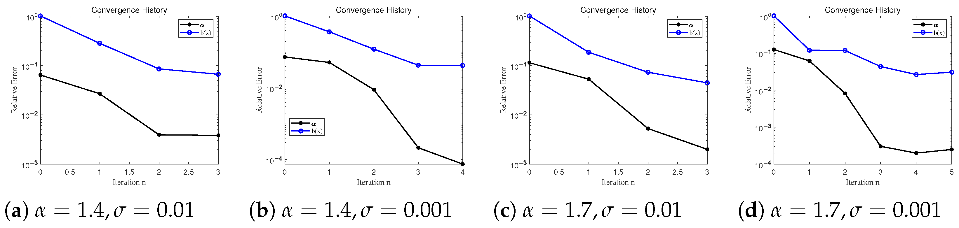
The accuracy of the evaluation results is quantified via the relative error formulas below:

$$e_{{\alpha }_n}={\displaystyle \frac{\left|{\overline{\alpha }}_n-{\alpha }^{*}\right|}{\left|{\alpha }^{*}\right|}},e_{b_n}={\displaystyle \frac{{\parallel {\overline{b}}_n-b^{*}\parallel }_2}{{\parallel b^{*}\parallel }_2}},$$

(56)

where n is the iteration index, ${\overline{\theta }}_n=\left({\overline{\alpha }}_n,{\overline{b}}_n\right)$ is the ensemble mean, and ${\theta }^{*}=\left({\alpha }^{*},b^{*}\right)$ denotes the exact parameter pair. The notation ${\parallel ·\parallel }_2$ corresponds to the conventional Euclidean vector norm.

Example 1.

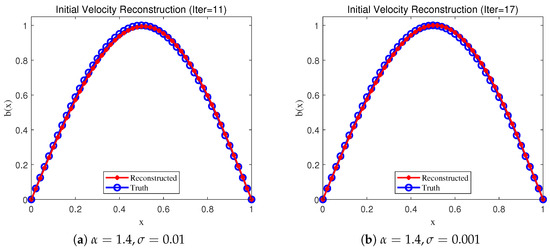
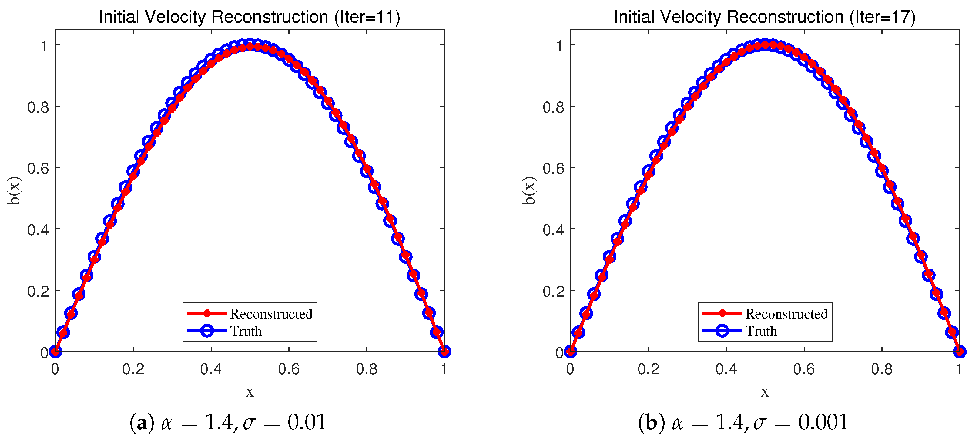
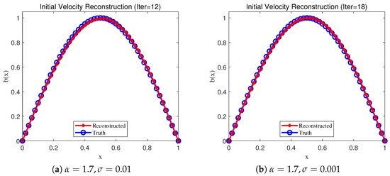
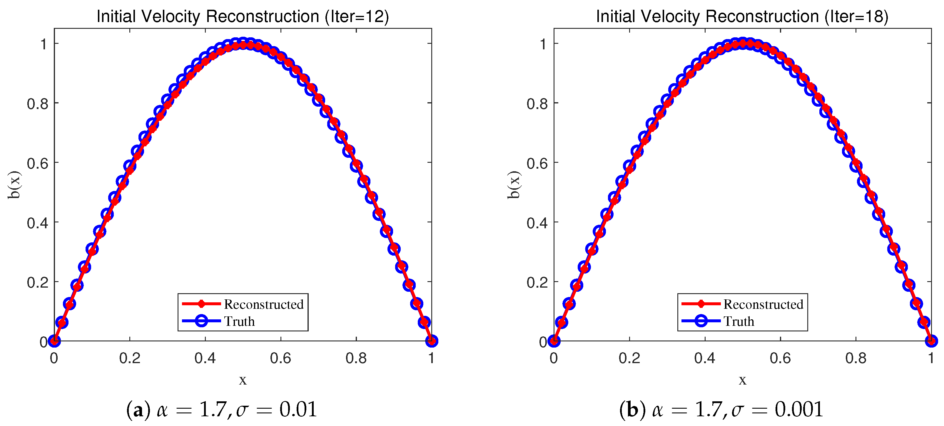
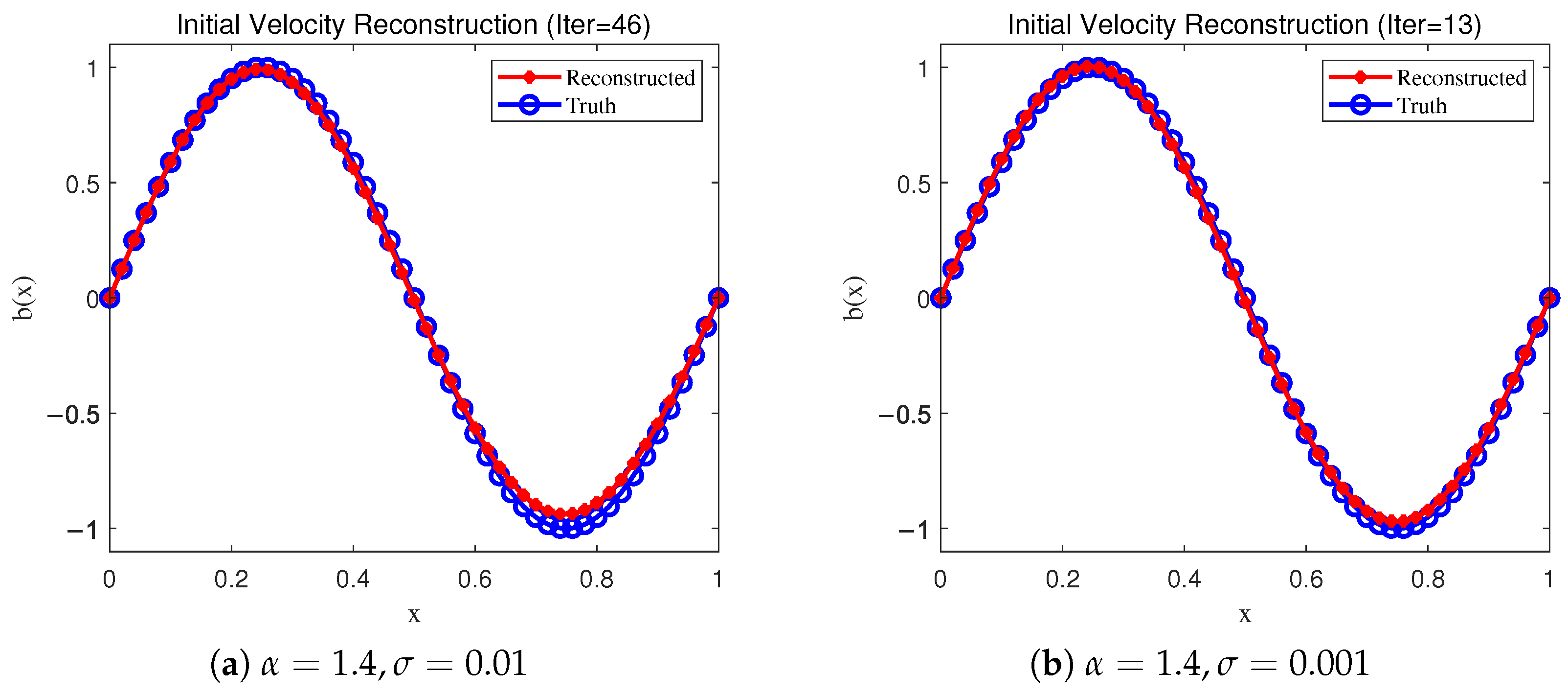
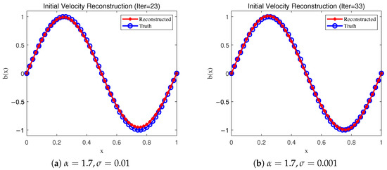
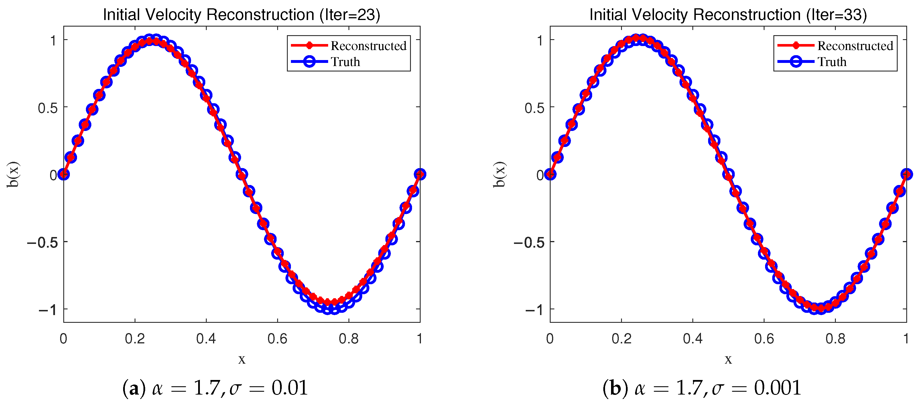
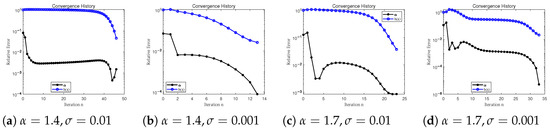
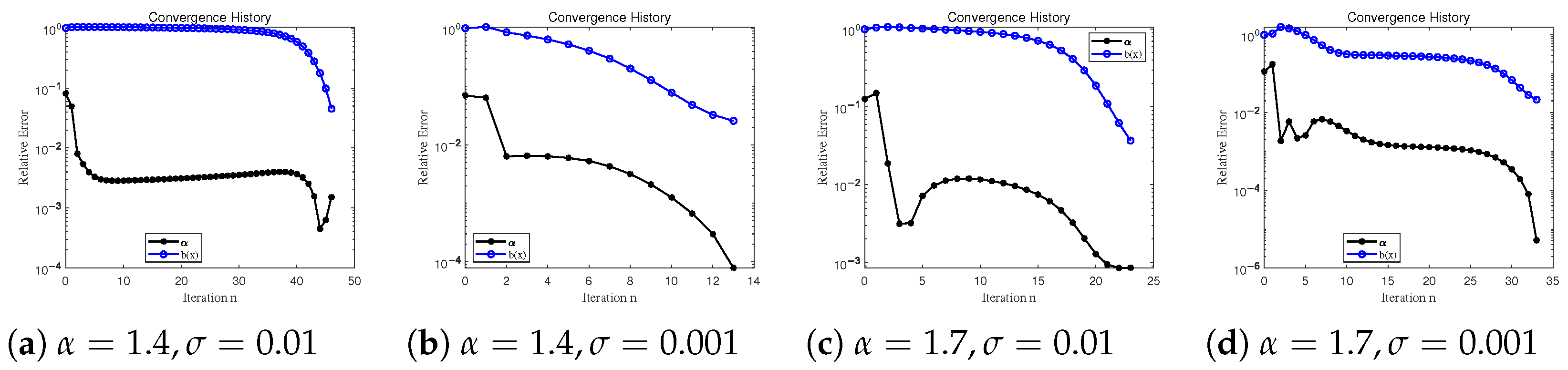
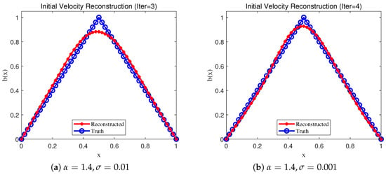
Choose $a\left(x\right)=x^2\sin \left(\pi x\right),b\left(x\right)=\sin \left(\pi x\right)$ for the initial data and $F\left(x,t\right)=\cos \left(\pi x\right)t$ for the source, with $K=10$, $\tau =1.01$, $\nu =0.7$, $s=3.5$, $N_e=200$. Using measurements at $x_0=25\pi /157$, we compute reconstructions for $\alpha =1.4$ and $\alpha =1.7$. Figure 1 and Figure 2 display these reconstructions in the same order; Figure 3 reports the relative errors.

Figure 1. Simulation results for Example 1 evaluated at $\alpha =1.4$.

Figure 2. Simulation results for Example 1 evaluated at $\alpha =1.7$.

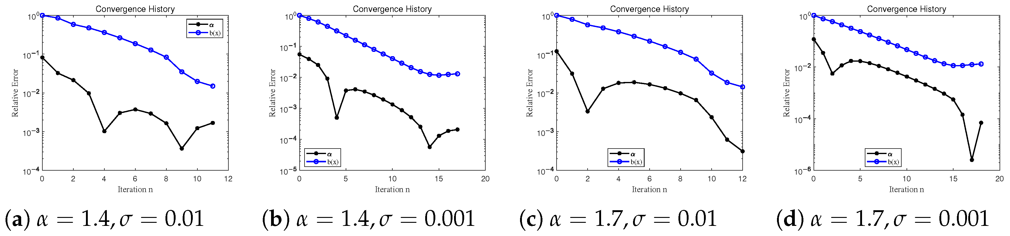
Figure 3. Relative errors of Example 1 with $\alpha =1.4$ and $\alpha =1.7$.

Example 2.

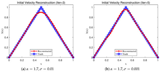
The second example uses $a\left(x\right)=x^2\sin \left(\pi x\right)$ and $b\left(x\right)=\sin \left(2\pi x\right)$ as initial data and prescribes $F\left(x,t\right)=\cos \left(\pi x\right)t$ as the source term. We set $K=10$, $\tau =1.01$, $\nu =0.1$, $s=4$, $N_e=200$. The interior measurements are taken at $x_0=25\pi /314$. The cases $\alpha =1.4$ and $\alpha =1.7$ are displayed in Figure 4 and Figure 5, respectively; their relative errors appear in Figure 6.

Figure 4. Simulation results for Example 2 evaluated at $\alpha =1.4$.

Figure 5. Simulation results for Example 2 evaluated at $\alpha =1.7$.

Figure 6. Relative errors of Example 2 with $\alpha =1.4$ and $\alpha =1.7$.

Example 3.

For the third example, take the initial data $a\left(x\right)=0$ and

$$b\left(x\right)=\left\{\begin{array}{cc}2x,\hfill & 0\le x<{\displaystyle \frac{1}{2}},\hfill \\ -2x+2,\hfill & {\displaystyle \frac{1}{2}}\le x\le 1\hfill \end{array}\right.$$

and the source $F\left(x,t\right)=\sin \left(\pi x\right)\cos \left(\pi t\right)$. Use $K=10$, $\tau =1.01$, $\nu =0.2$, $s=2.1$, $N_e=200$. Observations are collected at $x_0=25\pi /157$. Reconstruction results for $\alpha =1.4$ and $\alpha =1.7$ are given in Figure 7 and Figure 8; the corresponding error histories are plotted in Figure 9.

Figure 7. Simulation results for Example 3 evaluated at $\alpha =1.4$.

Figure 8. Simulation results for Example 3 evaluated at $\alpha =1.7$.

Figure 9. Relative errors of Example 3 with $\alpha =1.4$ and $\alpha =1.7$.

As shown in Figure 1, Figure 2, Figure 4, Figure 5, Figure 7 and Figure 8, the reconstructed initial velocity b agrees reasonably well with the exact solution. As illustrated in Figure 3, Figure 6 and Figure 9, the relative errors generally decrease during the iterations, although fluctuations may occur. These curves need not be monotone: the finite ensemble gives noisy covariance estimates, the nonlinear forward map couples the scalar order and the function-valued velocity, and the fixed perturbed observations contribute to variability across ensemble members. Thus, the discrepancy stopping rule controls the residual rather than enforcing monotone parameter errors. These findings indicate that IREKM can produce satisfactory reconstruction for the tested examples. The number of iterations varies with the example, the fractional order, and the noise level.

As shown in Table 1, Table 2 and Table 3, the IREKM results provide numerical evidence of robustness to measurement noise across the three examples. As the noise level $\sigma$ decreases from $0.05$ to $0.001$, the relative reconstruction errors for the initial velocity $b\left(x\right)$ and the fractional order $\alpha$ exhibit a general decrease. Notably, the scalar parameter $\alpha$ is reconstructed with exceptionally high precision in these tests, indicating accurate recovery from single-point interior measurements rather than a general accuracy guarantee.

Table 1. Computational outcomes across distinct noise magnitudes corresponding to Example 1.

$\mathit{\sigma }$	$\mathit{\alpha }$	${\overline{\mathit{\alpha }}}_{{\mathit{n}}_{*}}$	${\mathit{e}}_{{\overline{\mathit{\alpha }}}_{{\mathit{n}}_{*}}}$	${\mathit{e}}_{{\overline{\mathit{b}}}_{{\mathit{n}}_{*}}}$	${\mathit{n}}_{*}$
0.05	1.4	1.38981	0.007279	0.031444	6
0.01	1.4	1.39765	0.001679	0.014951	11
0.005	1.4	1.39876	0.000886	0.013415	13
0.001	1.4	1.39971	0.000207	0.013026	17
0.05	1.7	1.69679	0.001888	0.020440	7
0.01	1.7	1.69947	0.000312	0.014281	12
0.005	1.7	1.69962	0.000224	0.014204	14
0.001	1.7	1.69988	0.000071	0.013128	18

Table 2. Computational outcomes across distinct noise magnitudes corresponding to Example 2.

$\mathit{\sigma }$	$\mathit{\alpha }$	${\overline{\mathit{\alpha }}}_{{\mathit{n}}_{*}}$	${\mathit{e}}_{{\overline{\mathit{\alpha }}}_{{\mathit{n}}_{*}}}$	${\mathit{e}}_{{\overline{\mathit{b}}}_{{\mathit{n}}_{*}}}$	${\mathit{n}}_{*}$
0.05	1.4	1.38807	0.008521	0.338170	155
0.01	1.4	1.39787	0.001521	0.045116	46
0.005	1.4	1.39945	0.000393	0.044340	27
0.001	1.4	1.40011	0.000079	0.025869	13
0.05	1.7	1.69036	0.005671	0.150347	84
0.01	1.7	1.69854	0.000859	0.036959	23
0.005	1.7	1.69959	0.000241	0.032626	16
0.001	1.7	1.70001	0.000006	0.021549	33

Table 3. Computational outcomes across distinct noise magnitudes corresponding to Example 3.

$\mathit{\sigma }$	$\mathit{\alpha }$	${\overline{\mathit{\alpha }}}_{{\mathit{n}}_{*}}$	${\mathit{e}}_{{\overline{\mathit{\alpha }}}_{{\mathit{n}}_{*}}}$	${\mathit{e}}_{{\overline{\mathit{b}}}_{{\mathit{n}}_{*}}}$	${\mathit{n}}_{*}$
0.05	1.4	1.38497	0.010736	0.118340	2
0.01	1.4	1.39463	0.003836	0.066978	3
0.005	1.4	1.39766	0.001671	0.045593	4
0.001	1.4	1.40011	0.000079	0.042656	4
0.05	1.7	1.69248	0.004424	0.105348	2
0.01	1.7	1.70339	0.001994	0.044790	3
0.005	1.7	1.70146	0.000859	0.042447	4
0.001	1.7	1.70042	0.000247	0.030771	5

In these tests, IREKM provides a satisfactory joint reconstruction of the initial velocity and the fractional order for the time-fractional diffusion-wave model.

We compare IREKM with classical Tikhonov regularization in Example 1, using the same forward solver, computational grids, observation point and times, and realization of the noisy data d. Writing b for the vector of nodal values of the initial velocity, we consider the following discrete Tikhonov regularization functional

$${\mathcal{J}}_{\kappa }(\alpha ,b)={\displaystyle \frac{1}{2}}{∥{\mathcal{G}}_{h,\Delta t}(\alpha ,b)-d∥}_2^2+{\displaystyle \frac{\kappa }{2}}{\parallel b\parallel }_2^2,$$

(57)

where $\kappa >0$ is the discrete regularization parameter and ${\parallel ·\parallel }_2$ denotes the Euclidean norm. The corresponding minimization problem is

$$({\alpha }_{\kappa },b_{\kappa })\in \underset{\begin{array}{c}\alpha \in I_{\alpha },b\in {\mathbb{R}}^{N_x+1}\\ b_0=b_{N_x}=0\end{array}}{\arg \min }{\mathcal{J}}_{\kappa }(\alpha ,b).$$

(58)

For each fixed $\alpha$, the forward map is affine in b, and the conjugate gradient method solves the regularized normal equations to obtain $b_{\kappa }\left(\alpha \right)$. An outer bounded one-dimensional derivative-free search is used to minimize ${\mathcal{J}}_{\kappa }\left(\alpha ,b_{\kappa }\left(\alpha \right)\right)$ over $I_{\alpha }$.

The two methods are compared using the relative reconstruction errors defined above and CPU time with $\alpha =1.5$ and $\alpha =1.6$. In the following comparative experiments, we use the same parameter values for the IREKM method as in Example 1. For the Tikhonov regularization method, we set the regularization parameter $\kappa$ to $2.5\times {10}^{-3}$, $7.4\times {10}^{-4}$, $2.9\times {10}^{-4}$, $4.6\times {10}^{-5}$, and $4.2\times {10}^{-6}$ for $\sigma =0.05$, $0.01$, $0.005$, $0.001$, and $0.0001$, respectively. The relative errors of the regularized numerical solutions obtained using the two methods and the corresponding CPU times are reported in Table 4 and Table 5.

Table 4. Numerical comparison of IREKM and the classical Tikhonov regularization approach for Example 1 with $\alpha =1.5$ at various noise levels.

Method	$\mathit{\sigma }$	${\mathit{e}}_{\mathit{\alpha }}$	${\mathit{e}}_{\mathit{b}}$	${\mathit{t}}_{\mathit{CPU}}$
IREKM	0.05	0.006527	0.024458	329.2813
Tikhonov		0.001650	0.141330	5.6719
IREKM	0.01	0.001540	0.016598	535.3281
Tikhonov		0.000513	0.090770	4.7500
IREKM	0.005	0.000833	0.012627	711.0781
Tikhonov		0.000027	0.065905	4.9219
IREKM	0.001	0.000153	0.014370	1025.4753
Tikhonov		0.000026	0.021617	4.7188
IREKM	0.0001	0.000013	0.014780	1418.9611
Tikhonov		0.000003	0.006211	4.6719

Table 5. Numerical comparison of IREKM and the classical Tikhonov regularization approach for Example 1 with $\alpha =1.6$ at various noise levels.

Method	$\mathit{\sigma }$	${\mathit{e}}_{\mathit{\alpha }}$	${\mathit{e}}_{\mathit{b}}$	${\mathit{t}}_{\mathit{CPU}}$
IREKM	0.05	0.004381	0.021848	439.2188
Tikhonov		0.001346	0.122887	4.5625
IREKM	0.01	0.001050	0.013592	745.4375
Tikhonov		0.001362	0.070038	4.5469
IREKM	0.005	0.000450	0.014899	766.4219
Tikhonov		0.000451	0.048870	4.7500
IREKM	0.001	0.000094	0.011991	1073.2344
Tikhonov		0.000059	0.021166	4.9844
IREKM	0.0001	0.000013	0.013121	1485.2707
Tikhonov		0.000005	0.006595	4.7656

Table 4 and Table 5 show that both methods accurately estimate the fractional order $\alpha$, with Tikhonov regularization yielding smaller errors in most cases. IREKM requires substantially more CPU time than the Tikhonov implementation in every reported test. Its CPU time increases as $\sigma$ decreases, whereas the Tikhonov timings remain relatively stable. For the initial velocity $b\left(x\right)$, IREKM achieves smaller errors at the tested noise levels from $\sigma =0.05$ to $0.001$, whereas Tikhonov regularization is more accurate at $\sigma =0.0001$. The initial velocity errors of IREKM do not decrease consistently as the noise level decreases, indicating different accuracy and computational cost trade-offs between the two methods.

A key feature of IREKM is its derivative-free joint reconstruction of $\alpha$ and $b\left(x\right)$ through forward model evaluations and empirical ensemble covariances. In particular, it avoids the difficulties associated with deriving and numerically evaluating derivatives of the forward operator with respect to $\alpha$. The Tikhonov implementation used here also avoids differentiation with respect to $\alpha$ through an outer derivative-free search; thus, this feature is not exclusive to IREKM in the present comparison.

6. Conclusions

This work investigates the simultaneous recovery of the fractional order and initial velocity in a one-dimensional time-fractional diffusion-wave equation from a single interior time trace. With the source term and initial displacement prescribed, uniqueness is established through short-time asymptotic analysis, Laplace transforms, and spectral analysis. Within a Bayesian framework, we establish posterior existence and stability with respect to the data, together with convergence of the approximate posterior under an assumed forward-solver error bound. Numerical reconstruction is performed using IREKM, a derivative-free method that avoids differentiation with respect to the fractional order. Three numerical examples demonstrate the effectiveness and stability of the algorithm used in this work.

The uniqueness analysis considers $\alpha \in (1,2)$ and $b\in D\left({(-\Delta )}^{{\gamma }_2}\right)$ with ${\gamma }_2>3/4$, whereas the Bayesian formulation uses the parameter space $I_{\alpha }\times L^2(0,l)$, with $I_{\alpha }$ a compact subinterval of $(1,2)$. The present analysis is restricted to one spatial dimension with a prescribed source and initial displacement, and does not provide an IREKM convergence rate or a general small-noise error bound. In higher dimensions, repeated eigenvalues and eigenfunctions vanishing at the observation point may obstruct recovery from a single interior time trace, potentially requiring additional observations or suitable observability assumptions. Larger spatial discretizations and fractional memory terms also increase the computational and storage costs of ensemble forward simulations. Future work will investigate these theoretical issues and higher-dimensional extensions, while exploring parallel implementations, reduced-order models, and neural-network-based forward solvers to improve computational efficiency.

References

- Berkowitz, B.; Scher, H.; Silliman, S.E. Anomalous transport in laboratory-scale, heterogeneous porous media. Water Resour. Res. 2000, 36, 149–158. [Google Scholar] [CrossRef] [Scilit]
- Metzler, R.; Barkai, E.; Klafter, J. Anomalous diffusion and relaxation close to thermal equilibrium: A fractional Fokker-Planck equation approach. Phys. Rev. Lett. 1999, 82, 3563–3567. [Google Scholar] [CrossRef] [Scilit]
- Metzler, R.; Klafter, J. Subdiffusive transport close to thermal equilibrium: From the Langevin equation to fractional diffusion. Phys. Rev. E 2000, 61, 6308–6311. [Google Scholar] [CrossRef] [Scilit] [PubMed]
- Boggs, J.M.; Young, S.C.; Beard, L.M.; Gelhar, L.W.; Rehfeldt, K.R.; Adams, E.E. Field study of dispersion in a heterogeneous aquifer. Water Resour. Res. 1992, 28, 3281–3291. [Google Scholar] [CrossRef] [Scilit]
- Mainardi, F. Fractional Calculus and Waves in Linear Viscoelasticity: An Introduction to Mathematical Models, 2nd ed.; World Scientific: Singapore, 2022. [Google Scholar]
- Nigmatullin, R.R. The realization of the generalized transfer equation in a medium with fractal geometry. Phys. Status Solidi B 1986, 133, 425–430. [Google Scholar] [CrossRef] [Scilit]
- Sokolov, I.M.; Klafter, J. From diffusion to anomalous diffusion: A century after Einstein’s Brownian motion. Chaos 2005, 15, 026103. [Google Scholar] [CrossRef] [Scilit] [PubMed]
- Sakamoto, K.; Yamamoto, M. Initial value/boundary value problems for fractional diffusion-wave equations and applications to some inverse problems. J. Math. Anal. Appl. 2011, 382, 426–447. [Google Scholar] [CrossRef] [Scilit]
- Podlubny, I. Fractional Differential Equations: An Introduction to Fractional Derivatives, Fractional Differential Equations, to Methods of Their Solution and Some of Their Applications; Mathematics in Science and Engineering; Academic Press: San Diego, CA, USA, 1999; Volume 198. [Google Scholar]
- Agrawal, O.P. Solution for a fractional diffusion-wave equation defined in a bounded domain. Nonlinear Dyn. 2002, 29, 145–155. [Google Scholar] [CrossRef] [Scilit]
- Jin, B.; Lazarov, R.; Zhou, Z. Two fully discrete schemes for fractional diffusion and diffusion-wave equations with nonsmooth data. SIAM J. Sci. Comput. 2016, 38, A146–A170. [Google Scholar] [CrossRef] [Scilit]
- Gorenflo, R.; Luchko, Y.; Yamamoto, M. Time-fractional diffusion equation in the fractional Sobolev spaces. Fract. Calc. Appl. Anal. 2015, 18, 799–820. [Google Scholar] [CrossRef] [Scilit]
- Liu, Y.; Rundell, W.; Yamamoto, M. Strong maximum principle for fractional diffusion equations and an application to an inverse source problem. Fract. Calc. Appl. Anal. 2016, 19, 888–906. [Google Scholar] [CrossRef] [Scilit]
- Jiang, H.; Liu, F.; Turner, I.; Burrage, K. Analytical solutions for the multi-term time-fractional diffusion-wave/diffusion equations in a finite domain. Comput. Math. Appl. 2012, 64, 3377–3388. [Google Scholar] [CrossRef] [Scilit]
- Sabermahani, S.; Ordokhani, Y.; Hassani, H. General Lagrange scaling functions: Application in general model of variable order fractional partial differential equations. Comput. Appl. Math. 2021, 40, 269. [Google Scholar] [CrossRef] [Scilit]
- Xian, J.; Wei, T. Determination of the initial data in a time-fractional diffusion-wave problem by a final time data. Comput. Math. Appl. 2019, 78, 2525–2540. [Google Scholar] [CrossRef] [Scilit]
- Yamamoto, M. Uniqueness in determining fractional orders of derivatives and initial values. Inverse Probl. 2021, 37, 095006. [Google Scholar] [CrossRef] [Scilit]
- Wei, T.; Deng, R. Simultaneous determination of the order and a coefficient in a fractional diffusion-wave equation. J. Sci. Comput. 2025, 103, 31. [Google Scholar] [CrossRef] [Scilit]
- Yang, F.; Li, R.H.; Gao, Y.X.; Li, X.X. Two regularization methods for identifying the source term of Caputo–Hadamard type time fractional diffusion-wave equation. J. Inverse Ill-Posed Probl. 2025, 33, 369–399. [Google Scholar] [CrossRef] [Scilit]
- Yan, L.L.; Yang, F.; Li, X.X. Identifying the random source term and two initial values simultaneously for the stochastic time-fractional diffusion–wave equation. Commun. Nonlinear Sci. Numer. Simul. 2026, 152, 109135. [Google Scholar] [CrossRef] [Scilit]
- Wei, T.; Xu, J.; Yue, X. Identifying the order and a space source term in a time fractional diffusion-wave equation. East Asian J. Appl. Math. 2026, 16, 168–203. [Google Scholar] [CrossRef] [Scilit]
- Chang, M.; Wei, T. Identification of the spatial dependent source and the fractional order in a time-fractional convection diffusion-wave equation. Inverse Probl. Imaging 2026, 20, 330–367. [Google Scholar] [CrossRef] [Scilit]
- Xian, J.; Chen, Y.; Zhang, L.; Xu, C. Recovering a space-dependent coefficient in a time fractional diffusion-wave equation via a Banach space regularization scheme. Mathematics 2026, 14, 2875. [Google Scholar] [CrossRef] [Scilit]
- Zhang, C. On the simultaneous recovery of the fractional order and a time-dependent source term in a time-fractional diffusion-wave equation. J. Appl. Math. Comput. 2026, 72, 183. [Google Scholar] [CrossRef] [Scilit]
- Xian, J.; Yan, X.; Wei, T. Simultaneous identification of three parameters in a time-fractional diffusion-wave equation by a part of boundary Cauchy data. Appl. Math. Comput. 2020, 384, 125382. [Google Scholar] [CrossRef] [Scilit]
- Yan, X.; Zhang, Y.X.; Wei, T. Identify the fractional order and diffusion coefficient in a fractional diffusion wave equation. J. Comput. Appl. Math. 2021, 393, 113497. [Google Scholar] [CrossRef] [Scilit]
- Shiri, B.; Kong, H.; Wu, G.C.; Luo, C. Adaptive learning neural network method for solving time–fractional diffusion equations. Neural Comput. 2022, 34, 971–990. [Google Scholar] [CrossRef] [Scilit] [PubMed]
- Kilbas, A.A.; Srivastava, H.M.; Trujillo, J.J. Theory and Applications of Fractional Differential Equations; North-Holland Mathematics Studies; Elsevier: Amsterdam, The Netherlands, 2006; Volume 204. [Google Scholar]
- Jing, X.; Yamamoto, M. Simultaneous uniqueness for multiple parameters identification in a fractional diffusion-wave equation. Inverse Probl. Imaging 2022, 16, 1199–1217. [Google Scholar] [CrossRef] [Scilit]
- Freiling, G.; Yurko, V.A. Inverse Sturm-Liouville Problems and Their Applications; Nova Science Publishers: Huntington, NY, USA, 2001. [Google Scholar]
- Kaipio, J.P.; Somersalo, E. Statistical and Computational Inverse Problems; Springer: New York, NY, USA, 2005. [Google Scholar]
- Stuart, A.M. Inverse problems: A Bayesian perspective. Acta Numer. 2010, 19, 451–559. [Google Scholar] [CrossRef] [Scilit]
- Dashti, M.; Stuart, A.M. The Bayesian approach to inverse problems. In Handbook of Uncertainty Quantification; Ghanem, R., Higdon, D., Owhadi, H., Eds.; Springer: Cham, Switzerland, 2017; pp. 311–428. [Google Scholar]
- Cotter, S.L.; Dashti, M.; Stuart, A.M. Approximation of Bayesian inverse problems for PDEs. SIAM J. Numer. Anal. 2010, 48, 322–345. [Google Scholar] [CrossRef] [Scilit]
- Dashti, M.; Stuart, A.M. Uncertainty quantification and weak approximation of an elliptic inverse problem. SIAM J. Numer. Anal. 2011, 49, 2524–2542. [Google Scholar] [CrossRef] [Scilit]
- Evensen, G. The ensemble Kalman filter: Theoretical formulation and practical implementation. Ocean Dyn. 2003, 53, 343–367. [Google Scholar] [CrossRef] [Scilit]
- Iglesias, M.A.; Law, K.J.H.; Stuart, A.M. Ensemble Kalman methods for inverse problems. Inverse Probl. 2013, 29, 045001. [Google Scholar] [CrossRef] [Scilit]
- Iglesias, M.A. A regularizing iterative ensemble Kalman method for PDE-constrained inverse problems. Inverse Probl. 2016, 32, 025002. [Google Scholar] [CrossRef] [Scilit]
- Chada, N.K.; Iglesias, M.A.; Roininen, L.; Stuart, A.M. Parameterizations for ensemble Kalman inversion. Inverse Probl. 2018, 34, 055009. [Google Scholar] [CrossRef] [Scilit]
- Chada, N.K.; Stuart, A.M.; Tong, X.T. Tikhonov regularization within ensemble Kalman inversion. SIAM J. Numer. Anal. 2020, 58, 1263–1294. [Google Scholar] [CrossRef] [Scilit]
- Sun, Z.; Wu, X. A fully discrete difference scheme for a diffusion-wave system. Appl. Numer. Math. 2006, 56, 193–209. [Google Scholar] [CrossRef] [Scilit]
Disclaimer/Publisher’s Note: The statements, opinions and data contained in all publications are solely those of the individual author(s) and contributor(s) and not of MDPI and/or the editor(s). MDPI and/or the editor(s) disclaim responsibility for any injury to people or property resulting from any ideas, methods, instructions or products referred to in the content. |
© 2026 by the authors. Licensee MDPI, Basel, Switzerland. This article is an open access article distributed under the terms and conditions of the Creative Commons Attribution (CC BY) license.