Hooks and Hockey Sticks on the Catalan Triangle

Abstract

The inverse of the coefficient matrix of the Chebyshev S-polynomials is the Catalan triangle. From this inverse matrix, we derive rules in the spirit of Pascal’s rule in three distinct senses. First, there is a local hook rule: each entry is generated from two entries one row up, and a similar local rule governs the symmetric matrix $\mathcal{S}{\mathcal{S}}^T$. Second, there is a cumulative rule: an exact analogue of the classical hockey stick identity, in which a sum of consecutive entries along an anti-diagonal telescopes to a single entry of the matrix. Third, there is a row-by-row relation: the row polynomials of the inverse matrix satisfy a linear recurrence weighted by Catalan numbers, informally a symbolic inverse of the original recurrence. The same hook rule also yields a Catalan-weighted identity linking the rows of the inverse matrix to the S-polynomials.

1. Introduction

Writing a polynomial family in matrix form, and studying the inverse of the resulting coefficient matrix, is a recurring theme in the literature on special polynomial sequences. Falcón and Plaza [1], for instance, examined the coefficient matrix arising from the k-Fibonacci polynomials and derived identities from the rows of its inverse. Barry [2,3] investigated families of Pascal-like matrices defined by Riordan arrays. He studied their inverses and central coefficients. Moghaddamfar and Pooya [4] studied generalized Pascal triangles through matrix factorizations. In [5], a triangular matrix attached to the Chebyshev polynomials of the second kind $U_n\left(x\right)$ and its inverse are modelled and studied through the relation between the derivatives and the powers of the generating function of these polynomials. The entries of the inverse matrix are, up to sign, ballot numbers, and Qi, Zou, and Guo derived several identities for the Catalan numbers from them. Agapito et al. [6] showed that Shapiro’s Catalan triangle is the change-of-basis matrix between the monomials and the shifted Chebyshev polynomials $U_n\left({\displaystyle \frac{x-2}{2}}\right)$, that is, the inverse of their coefficient matrix. Barry [7] used the Riordan array $\left({\displaystyle \frac{1}{1+x^2}},{\displaystyle \frac{x}{1+x^2}}\right)$, which is the matrix $\mathcal{S}$ studied here, together with Pascal’s triangle to construct the RNA involution in the Riordan group. At a more general level, He [8] showed that, for any orthogonal polynomial family, the production matrix of the inverse coefficient matrix is the Jacobi matrix of its three-term recurrence. More broadly, recurrences whose coefficients are built from Catalan numbers are a productive source of integer sequences elsewhere in the literature. A notable recent instance is Lassalle’s proof [9] of a Zeilberger conjecture on two such sequences, obtained via symmetric functions and continued fractions.

The classical hockey stick identity has also been extended in several directions. Donley [10] introduced binomial arrays, which extend Pascal’s triangle to columns with negative indices. He gave nine hockey stick rules for these arrays and displayed each one as a pattern of boxed entries in a small matrix. Some rules sum along a column, some along a row, and some along a diagonal; some alternate in sign. Lynch and Weselcouch [11] summed binomial coefficients along lines of other slopes in Pascal’s triangle and proved the resulting identity by a sign-reversing involution.

The objective of this paper is to present an infinite matrix: the coefficient matrix $\mathcal{S}$ of the Chebyshev S-polynomials ${\left\{S_n\left(x\right)\right\}}_{n\ge 0}$, defined by

$$S_n\left(x\right)=U_n\left({\displaystyle \frac{x}{2}}\right),$$

(1)

where $U_n$ is the Chebyshev polynomial of the second kind of degree n, given by $U_n\left(\cos \theta \right)=\sin \left((n+1)\theta \right)/\sin \theta$ [12], together with its inverse ${\mathcal{S}}^{-1}$ and the symmetric product $\mathcal{W}=\mathcal{S}{\mathcal{S}}^T$. The polynomials $S_n$ are monic with integer coefficients and satisfy the three-term recurrence

$$S_n\left(x\right)=x{S}_{n-1}\left(x\right)-S_{n-2}\left(x\right),S_{-1}=0,S_0=1;$$

(2)

writing the system ${\left(S_0\left(x\right),S_1\left(x\right),S_2\left(x\right),\dots \right)}^T=\mathcal{S}{\left(1,x,x^2,\dots \right)}^T$ defines $\mathcal{S}$ as an infinite unit lower triangular integer matrix.

The Chebyshev origin of $\mathcal{S}$ is thus the source of our object of study. The results below concern the combinatorial structure of $\mathcal{S}$, ${\mathcal{S}}^{-1}$, and $\mathcal{W}$ as matrices in their own right, and are stated accordingly. Our contributions are the following:

(i)

The entries $t_{i,j}$ of ${\mathcal{S}}^{-1}$ satisfy the hook rule

$$t_{i,j}=t_{i-1,j-1}+t_{i-1,j+1},$$

(3)

a symmetric analogue of Pascal’s rule $\left({\displaystyle \genfrac{}{}{0pt}{}{i}{j}}\right)=\left({\displaystyle \genfrac{}{}{0pt}{}{i-1}{j-1}}\right)+\left({\displaystyle \genfrac{}{}{0pt}{}{i-1}{j}}\right)$ (Theorem 1), for which we give an elementary binomial proof.

(ii)

The hook rule along a line of constant $i+j$ gives a hockey-stick-type identity,

$${\displaystyle \sum _{k=0}^n}{t}_{i+k,i-k}=t_{i+n+1,i-n+1}(i\ge 1,0\le n\le i),$$

(4)

an exact structural analogue of the classical hockey stick identity ${\sum }_{k=0}^n\left({\displaystyle \genfrac{}{}{0pt}{}{i+k}{i}}\right)=\left({\displaystyle \genfrac{}{}{0pt}{}{i+n+1}{i+1}}\right)$ on Pascal’s triangle (Corollary 1, Section 6), valid here only up to $n=i$, where the sum collapses to the Catalan number $C_i$.

(iii)

The hook rule also proves a second identity. Pairing row n of ${\mathcal{S}}^{-1}$ with the shifted family $S_1,\dots ,S_n$, instead of the family $S_0,\dots ,S_{n-1}$ used in the classical expansion of monomials, yields

$${\displaystyle \sum _{k=1}^n}{t}_{n,k}{S}_k\left(x\right)=x^n-{\displaystyle \sum _{k=1}^{\lfloor n/2\rfloor }}{C}_{k-1}{x}^{n-2k},$$

(5)

where $C_k={\displaystyle \frac{1}{k+1}}\left({\displaystyle \genfrac{}{}{0pt}{}{2k}{k}}\right)$ is the k-th Catalan number (Theorem 2). The Catalan numbers appear here as coefficients of a correction term, not as coefficients of $x^n$ itself.

(iv)

The row polynomials $T_n\left(p\right)={\sum }_{k=1}^n{t}_{n,k}{p}^{k-1}$ of ${\mathcal{S}}^{-1}$ satisfy the Catalan-weighted linear recurrence

$$T_n\left(p\right)=p{T}_{n-1}\left(p\right)+\sum _{i\ge 1}{C}_{i-1}{T}_{n-2i}\left(p\right)(n\ge 2),$$

(6)

which we prove in closed form from the Riordan representation of ${\mathcal{S}}^{-1}$ (Theorem 3, Section 8).

(v)

The symmetric matrix $\mathcal{W}=\mathcal{S}{\mathcal{S}}^T$ satisfies the local cross rule

$${\mathcal{W}}_{i,j}={\mathcal{W}}_{i-1,j-1}+{\mathcal{W}}_{i-1,j+1}+{\mathcal{W}}_{i+1,j-1}+{\mathcal{W}}_{i+1,j+1}(i,j\ge 2),$$

i.e., every entry equals the sum of its four diagonal neighbours (Proposition 2); rotated by ${45}^{\circ }$, this becomes a honeycomb-type relation.

To our knowledge, items (iii), (iv) and (v) have not appeared before. Item (ii) is, after a change in indices, the partial sum property of Catalan’s triangle [13]; we include it because, inside ${\mathcal{S}}^{-1}$, it takes the shape of a hockey stick and follows from the hook rule alone. The hook rule (i) is known (Remark 4); what we add is an elementary proof and its use as a proof device. Theorem 3 gives a proof of the recurrence (iv), whose underlying generating function was stated in an earlier comment by the author and Lang [14]. The Riordan representation ${\mathcal{S}}^{-1}=\left(c\left(x^2\right),xc\left(x^2\right)\right)$ (Proposition 3), with c as the Catalan generating function, goes back to Lang [15]; we use it only as a tool.

The rest of this paper is organized as follows. Section 2 collects the necessary background on the S-polynomials, generating functions, and Riordan arrays. Section 3 introduces the coefficient matrix $\mathcal{S}$, its Riordan representation, and its connection to path graphs and to the Fibonacci polynomials. Section 4 discusses the Gram matrix $\mathcal{W}=\mathcal{S}{\mathcal{S}}^T$. Section 5 contains the hook rule and its proof, as well as the Riordan and convolution descriptions of ${\mathcal{S}}^{-1}$. Section 6 derives the hockey stick corollary from the hook rule and illustrates it with an example. Section 7 proves the Catalan identity (5), Section 8 proves the row polynomial recurrence (6), and Section 9 closes with some remarks and open questions.

2. Preliminaries

2.1. Chebyshev S-Polynomials

From the recurrence (2), the first members of the family are

$$\begin{array}{cccc}\hfill S_0\left(x\right)& =1,\hfill & \hfill S_1\left(x\right)& =x,\hfill \\ \hfill S_2\left(x\right)& =x^2-1,\hfill & \hfill S_3\left(x\right)& =x^3-2x,\hfill \\ \hfill S_4\left(x\right)& =x^4-3x^2+1,\hfill & \hfill S_5\left(x\right)& =x^5-4x^3+3x,\hfill \\ \hfill S_6\left(x\right)& =x^6-5x^4+6x^2-1,\hfill & \hfill S_7\left(x\right)& =x^7-6x^5+10x^3-4x,\hfill \\ \hfill S_8\left(x\right)& =x^8-7x^6+15x^4-10x^2+1,\hfill & \hfill S_9\left(x\right)& =x^9-8x^7+21x^5-20x^3+5x.\hfill \end{array}$$

The ordinary generating function of the family is obtained by summing the recurrence (2): writing $g\left(z\right)={\sum }_{n\ge 0}{S}_n\left(x\right)z^n$, one finds

$$g\left(z\right)={\displaystyle \frac{1}{1-xz+z^2}}.$$

(7)

Indeed, substituting $xz-z^2$ into the geometric series ${\displaystyle \frac{1}{1-u}}={\sum }_{k\ge 0}{u}^k$ and collecting powers of z gives $1+xz+(x^2-1)z^2+(x^3-2x)z^3+\cdots ={\sum }_{n\ge 0}{S}_n\left(x\right)z^n$.

2.2. Catalan Numbers

The Catalan numbers

$$C_n={\displaystyle \frac{1}{n+1}}\left({\displaystyle \genfrac{}{}{0pt}{}{2n}{n}}\right),n=0,1,2,\dots ,$$

begin with $1,1,2,5,14,42,132,429,\dots$ (https://oeis.org/A000108, accessed on 20 August 2026) and are typically found in enumerative combinatorics [16]. Their ordinary generating function

$$c\left(x\right)=\sum _{n\ge 0}{C}_n{x}^n={\displaystyle \frac{1-\sqrt{1-4x}}{2x}}$$

(8)

satisfies the quadratic relation

$$c\left(x\right)=1+xc{\left(x\right)}^2.$$

(9)

The aerated Catalan sequence $1,0,1,0,2,0,5,0,14,\dots$ (https://oeis.org/A126120, accessed on 20 August 2026) has a generating function $c\left(x^2\right)$.

2.3. Convolution and Riordan Arrays

Given two generating functions $A\left(x\right)={\sum }_{n\ge 0}{a}_n{x}^n$ and $B\left(x\right)={\sum }_{n\ge 0}{b}_n{x}^n$, their product is the generating function of the convolution (Cauchy product)

$$c_n={\displaystyle \sum _{k=0}^n}{a}_k{b}_{n-k}$$

of the two coefficient sequences [17].

The Riordan group [18] is a set of infinite lower triangular integer matrices, where each matrix is defined by a pair of generating functions $G\left(x\right)=1+g_{1}x+g_2{x}^2+\cdots$ and $F\left(x\right)=f_{1}x+f_2{x}^2+\cdots$, where $f_1\ne 0$. The Riordan arrays have since become a standard tool of enumerative combinatorics [19,20,21,22]. The Riordan array $R=(G,F)$ is the lower triangular matrix whose j-th column ($j=0,1,2,\dots$) has a generating function

$$G\left(x\right)F{\left(x\right)}^j.$$

Under the multiplication rule

$$(G,F)·(H,L)=\left(G·(H\circ F),L\circ F\right)$$

the set of Riordan arrays forms a group—the Riordan group. The identity for this law is $I=(1,x)$, and the inverse

$${(G,F)}^{-1}=\left({\displaystyle \frac{1}{G\circ \overline{F}}},\overline{F}\right),$$

(10)

where $\overline{F}$ is the compositional inverse of F, that is, $F\left(\overline{F}\left(x\right)\right)=\overline{F}\left(F\left(x\right)\right)=x$. The classical example is Pascal’s triangle, $P=\left({\displaystyle \frac{1}{1-x}},{\displaystyle \frac{x}{1-x}}\right)$. We shall also use the fundamental theorem of Riordan arrays (FTRA): if M is the matrix $M:=(G,F)$, and $\mathbf{a}={(a_0,a_1,...,)}^T$ is an integer sequence with an ordinary generating function $A\left(x\right)$, then the sequence $M\mathbf{a}$ has an ordinary generating function $G\left(x\right)A\left(F\right(x\left)\right)$ [19,22].

3. The Coefficient Matrix $\mathcal{S}$

Let the polynomials of the family ${\left\{S_n\left(x\right)\right\}}_{n\ge 0}$ be transferred to matrix form. The resulting linear system

$$\mathbf{S}=\mathcal{S}X,\mathbf{S}={\left(S_0\left(x\right),S_1\left(x\right),S_2\left(x\right),\dots \right)}^T,X={\left(1,x,x^2,\dots \right)}^T,$$

(11)

defines the infinite lower triangular coefficient matrix $\mathcal{S}$. Throughout, we reserve the calligraphic $\mathcal{S}$ for this matrix and the plain $S_n\left(x\right)$ for the polynomials to avoid ambiguity between the two. Indexing rows and columns from 1, so that row i carries the coefficients of $S_{i-1}\left(x\right)$ arranged by increasing powers of x, the upper-left $12\times 12$ corner of $\mathcal{S}$ is

$$\mathcal{S}=\left(\begin{array}{cccccccccccc}\hfill 1& & & & & & & & & & & \\ \hfill 0& \hfill 1& & & & & & & & & & \\ \hfill -1& \hfill 0& \hfill 1& & & & & & & & & \\ \hfill 0& \hfill -2& \hfill 0& \hfill 1& & & & & & & & \\ \hfill 1& \hfill 0& \hfill -3& \hfill 0& \hfill 1& & & & & & & \\ \hfill 0& \hfill 3& \hfill 0& \hfill -4& \hfill 0& \hfill 1& & & & & & \\ \hfill -1& \hfill 0& \hfill 6& \hfill 0& \hfill -5& \hfill 0& \hfill 1& & & & & \\ \hfill 0& \hfill -4& \hfill 0& \hfill 10& \hfill 0& \hfill -6& \hfill 0& \hfill 1& & & & \\ \hfill 1& \hfill 0& \hfill -10& \hfill 0& \hfill 15& \hfill 0& \hfill -7& \hfill 0& \hfill 1& & & \\ \hfill 0& \hfill 5& \hfill 0& \hfill -20& \hfill 0& \hfill 21& \hfill 0& \hfill -8& \hfill 0& \hfill 1& & \\ \hfill -1& \hfill 0& \hfill 15& \hfill 0& \hfill -35& \hfill 0& \hfill 28& \hfill 0& \hfill -9& \hfill 0& \hfill 1& \\ \hfill 0& \hfill -6& \hfill 0& \hfill 35& \hfill 0& \hfill -56& \hfill 0& \hfill 36& \hfill 0& \hfill -10& \hfill 0& \hfill 1\end{array}\right).$$

(12)

This triangle can be found at (https://oeis.org/A049310, accessed on 20 August 2026) in the On-Line Encyclopedia of Integer Sequences (OEIS), contributed and extensively documented by W. Lang [23]. The entries admit the following closed form.

Definition 1.

Let $\mathcal{S}={\left[a_{i,j}\right]}_{i,j\ge 1}$. Then, $a_{i,j}=0$ for $i<j$, and for $i\ge j$,

$$a_{i,j}=\left\{\begin{array}{cc}0,\hfill & i+j\mathit{odd},\hfill \\ {(-1)}^{{\displaystyle \frac{i-j}{2}}}\left({\displaystyle \genfrac{}{}{0pt}{}{\frac{i+j}{2}-1}{j-1}}\right),\hfill & i+j\mathit{even}.\hfill \end{array}\right.$$

(13)

Formula (13) is equivalent to the standard expansion

$$S_n\left(x\right)={\displaystyle \sum _{m=0}^{\lfloor n/2\rfloor }}{(-1)}^m\left({\displaystyle \genfrac{}{}{0pt}{}{n-m}{m}}\right)x^{n-2m}$$

of the Chebyshev polynomials [12,23], rewritten in matrix coordinates.

Proposition 1.

$\mathcal{S}$ is the Riordan array

$$\mathcal{S}=\left({\displaystyle \frac{1}{1+x^2}},{\displaystyle \frac{x}{1+x^2}}\right).$$

Proof. 

By (7), the bivariate generating function of the triangle is

$$\sum _{n\ge 0}{S}_n\left(t\right)x^n={\displaystyle \frac{1}{1-tx+x^2}}={\displaystyle \frac{1}{1+x^2}}·{\displaystyle \frac{1}{1-t{\displaystyle \frac{x}{1+x^2}}}}=\sum _{m\ge 0}{\displaystyle \frac{1}{1+x^2}}{\left({\displaystyle \frac{x}{1+x^2}}\right)}^m{t}^m,$$

so the generating function of column m (counting from $m=0$) is ${\displaystyle \frac{1}{1+x^2}}{\left({\displaystyle \frac{x}{1+x^2}}\right)}^m$, which is precisely the Riordan rule with $G\left(x\right)={\displaystyle \frac{1}{1+x^2}}$ and $F\left(x\right)={\displaystyle \frac{x}{1+x^2}}$. □

Remark 1.

The representation in Proposition 1 is a specialization of the general fact that the coefficient arrays of the orthogonal polynomial families defined by three-term recurrences with constant coefficients are ordinary Riordan arrays; see Barry [24] and ([22], Chapter 9).

Remark 2.

Since $S_n\left(x\right)=x{S}_{n-1}\left(x\right)-S_{n-2}\left(x\right)$, the substitution $x\mapsto ix$ turns this into the Fibonacci polynomial recurrence $F_{n+1}=x{F}_n+F_{n-1}$: explicitly, $S_{n-1}\left(x\right)={(-i)}^{n-1}{F}_n\left(ix\right)$. Consequently $\mathcal{S}$ is, up to this sign pattern, the coefficient matrix of the Fibonacci polynomials tabulated by Falcón and Plaza [1]. The results of Section 4, Section 5, Section 6, Section 7 and Section 8 are independent of this identification.

Remark 3.

In graph theory, $S_n\left(x\right)$ is the characteristic polynomial of the path graph $P_n$ on n vertices, whose adjacency matrix is the $n\times n$ tri-diagonal 0-1 matrix with ones on the sub- and superdiagonal [25]. Under this reading, $\mathcal{S}$ is the coefficient table of the characteristic polynomials of all path graphs at once.

4. The Gram Matrix $\mathcal{W}\mathbf{=}\mathcal{S}{\mathcal{S}}^T$

A product of the form $A{A}^T$ is called a Gram matrix. It carries structural information about the rows of A. Such products appear in two well-known settings. In factorization theory, a symmetric matrix is decomposed into triangular factors, as in the Cholesky factorization. In graph theory, an incidence matrix multiplied by its transpose encodes adjacency information. Those settings start from a symmetric matrix and look for its triangular factors. Here, we go the other way. We start from the explicit triangular matrix $\mathcal{S}$ and study the symmetric matrix it produces. The factorization $\mathcal{W}=\mathcal{S}{\mathcal{S}}^T$ costs us nothing: $\mathcal{S}$ is already at hand. It is this symmetric product that actually carries the interesting combinatorics.

The upper-left corner of $\mathcal{W}=\mathcal{S}{\mathcal{S}}^T$ is

$$\mathcal{W}=\left(\begin{array}{cccccccc}\hfill 1& \hfill 0& \hfill -1& \hfill 0& \hfill 1& \hfill 0& \hfill -1& \hfill 0\\ \hfill 0& \hfill 1& \hfill 0& \hfill -2& \hfill 0& \hfill 3& \hfill 0& \hfill -4\\ \hfill -1& \hfill 0& \hfill 2& \hfill 0& \hfill -4& \hfill 0& \hfill 7& \hfill 0\\ \hfill 0& \hfill -2& \hfill 0& \hfill 5& \hfill 0& \hfill -10& \hfill 0& \hfill 18\\ \hfill 1& \hfill 0& \hfill -4& \hfill 0& \hfill 11& \hfill 0& \hfill -24& \hfill 0\\ \hfill 0& \hfill 3& \hfill 0& \hfill -10& \hfill 0& \hfill 26& \hfill 0& \hfill -58\\ \hfill -1& \hfill 0& \hfill 7& \hfill 0& \hfill -24& \hfill 0& \hfill 63& \hfill 0\\ \hfill 0& \hfill -4& \hfill 0& \hfill 18& \hfill 0& \hfill -58& \hfill 0& \hfill 153\end{array}\right).$$

(14)

The matrix $\mathcal{W}$ is symmetric, has determinant 1 (as the product of two unit triangular matrices), and exhibits the checkerboard pattern inherited from $\mathcal{S}$: ${\mathcal{W}}_{i,j}=0$ whenever $i+j$ is odd. Its main diagonal

$$1,1,2,5,11,26,63,153,376,931,\dots$$

is the Whitney-type sequence (https://oeis.org/A051286, accessed on 20 August 2026); by construction, its n-th term is the sum of the squares of the coefficients of $S_{n-1}\left(x\right)$.

The most striking feature of $\mathcal{W}$, however, is a local one.

Proposition 2

(Cross rule). For all $i,j\ge 2$,

$${\mathcal{W}}_{i,j}={\mathcal{W}}_{i-1,j-1}+{\mathcal{W}}_{i-1,j+1}+{\mathcal{W}}_{i+1,j-1}+{\mathcal{W}}_{i+1,j+1}.$$

(15)

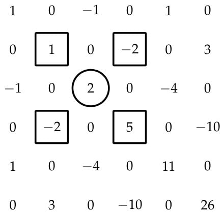
That is, every entry of $\mathcal{W}$ (off the first row and column) is the sum of its four diagonal neighbours.

Proof. 

Let $r_i=(a_{i,1},a_{i,2},a_{i,3},\dots )$ denote the i-th row of $\mathcal{S}$, a vector of finite support, and let $⟨·,·⟩$ be the standard inner product, so that ${\mathcal{W}}_{i,j}=⟨r_i,r_j⟩$. Let R be the right-shift operator, ${\left(Rv\right)}_k=v_{k-1}$ (with $v_0:=0$). Since R merely shifts coordinates, it preserves inner products: $⟨Ru,Rv⟩=⟨u,v⟩$. The recurrence (2) translates into the entry-wise rule

$$a_{i+1,k}=a_{i,k-1}-a_{i-1,k}(i\ge 2,k\ge 1,a_{i,0}:=0),$$

(16)

which, in terms of rows, reads

$$r_{i+1}=R{r}_i-r_{i-1}(i\ge 2).$$

(17)

Now, expand the four terms on the right-hand side of (15) using (17). Abbreviating $X=⟨R{r}_i,r_{j-1}⟩$ and $Y=⟨r_{i-1},R{r}_j⟩$,

$$\begin{array}{cc}\hfill {\mathcal{W}}_{i+1,j+1}& =⟨R{r}_i-r_{i-1},R{r}_j-r_{j-1}⟩={\mathcal{W}}_{i,j}-X-Y+{\mathcal{W}}_{i-1,j-1},\hfill \\ \hfill {\mathcal{W}}_{i+1,j-1}& =⟨R{r}_i-r_{i-1},r_{j-1}⟩=X-{\mathcal{W}}_{i-1,j-1},\hfill \\ \hfill {\mathcal{W}}_{i-1,j+1}& =⟨r_{i-1},R{r}_j-r_{j-1}⟩=Y-{\mathcal{W}}_{i-1,j-1}.\hfill \end{array}$$

Adding these three identities to ${\mathcal{W}}_{i-1,j-1}$, all X, Y, and ${\mathcal{W}}_{i-1,j-1}$ terms cancel out, and the sum collapses to ${\mathcal{W}}_{i,j}$, which is (15). □

Figure 1 illustrates Proposition 2; the circled entry ${\mathcal{W}}_{3,3}=2$ equals the sum of its four boxed diagonal neighbours.

Figure 1. The cross rule of Proposition 2 on a $6\times 6$ patch of $\mathcal{W}$.

5. The Inverse Matrix ${\mathcal{S}}^{\mathbf{-}\mathbf{1}}$ and the Hook Rule

We now turn to the inverse of the coefficient matrix. Write ${\mathcal{S}}^{-1}={\left[t_{i,j}\right]}_{i,j\ge 1}$. Since $\mathcal{S}$ is unit lower triangular, so is ${\mathcal{S}}^{-1}$: $t_{i,j}=0$ for $i<j$ and $t_{i,i}=1$. The upper-left corner of ${\mathcal{S}}^{-1}$ is

$${\mathcal{S}}^{-1}=\left(\begin{array}{cccccccccccc}\hfill 1& & & & & & & & & & & \\ \hfill 0& \hfill 1& & & & & & & & & & \\ \hfill 1& \hfill 0& \hfill 1& & & & & & & & & \\ \hfill 0& \hfill 2& \hfill 0& \hfill 1& & & & & & & & \\ \hfill 2& \hfill 0& \hfill 3& \hfill 0& \hfill 1& & & & & & & \\ \hfill 0& \hfill 5& \hfill 0& \hfill 4& \hfill 0& \hfill 1& & & & & & \\ \hfill 5& \hfill 0& \hfill 9& \hfill 0& \hfill 5& \hfill 0& \hfill 1& & & & & \\ \hfill 0& \hfill 14& \hfill 0& \hfill 14& \hfill 0& \hfill 6& \hfill 0& \hfill 1& & & & \\ \hfill 14& \hfill 0& \hfill 28& \hfill 0& \hfill 20& \hfill 0& \hfill 7& \hfill 0& \hfill 1& & & \\ \hfill 0& \hfill 42& \hfill 0& \hfill 48& \hfill 0& \hfill 27& \hfill 0& \hfill 8& \hfill 0& \hfill 1& & \\ \hfill 42& \hfill 0& \hfill 90& \hfill 0& \hfill 75& \hfill 0& \hfill 35& \hfill 0& \hfill 9& \hfill 0& \hfill 1& \\ \hfill 0& \hfill 132& \hfill 0& \hfill 165& \hfill 0& \hfill 110& \hfill 0& \hfill 44& \hfill 0& \hfill 10& \hfill 0& \hfill 1\end{array}\right).$$

(18)

${\mathcal{S}}^{-1}$ being a Catalan triangle was noted by Lang [15], who credits the observation to an anonymous referee. The matrix ${\mathcal{S}}^{-1}$ has also appeared in other guises; Bajunaid et al. [26] used it to relate certain function series arising from random walks on trees. Its non-zero entries also appear, up to sign, in the inverse matrix of Qi, Zou, and Guo [5]. Its first column is the aerated Catalan sequence

$$1,0,1,0,2,0,5,0,14,0,42,0,132,\dots .$$

In the OEIS, the full aerated triangle (18) can be found at https://oeis.org/A053121 (accessed on 20 August 2026), where the explicit formula

$$t_{i,j}={\displaystyle \frac{j}{i}}\left({\displaystyle \genfrac{}{}{0pt}{}{i}{\frac{i-j}{2}}}\right)·{\displaystyle \frac{1+{(-1)}^{i-j}}{2}}(1\le j\le i)$$

(19)

is recorded, in the equivalent $(n,k)=(i-1,j-1)$ parametrization, by Deutsch [27]; in particular, $t_{i,j}=0$ when $i-j$ is odd, and when $i-j$ is even, the entry is the ballot number ${\displaystyle \frac{j}{i}}\left({\displaystyle \genfrac{}{}{0pt}{}{i}{(i-j)/2}}\right)$.

5.1. The Hook Rule

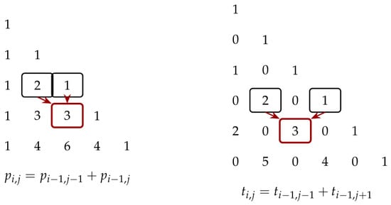
Pascal’s triangle, written as a lower triangular matrix $P=\left[p_{i,j}\right]=\left[\left({\displaystyle \genfrac{}{}{0pt}{}{i-1}{j-1}}\right)\right]$, is generated by Pascal’s rule

$$p_{i,j}=p_{i-1,j-1}+p_{i-1,j},$$

whose two terms form a hook (Figure 2, left). Our first main result is that ${\mathcal{S}}^{-1}$ is generated by a similar, but symmetric, hook.

Figure 2. The one-sided hook of Pascal’s rule (on the left) and the symmetric hook on ${\mathcal{S}}^{-1}$ (on the right).

Theorem 1 (Hook rule).

For $i\ge 2$ and $j\ge 1$, the entries of ${\mathcal{S}}^{-1}=\left[t_{i,j}\right]$ satisfy

$$t_{i,j}=t_{i-1,j-1}+t_{i-1,j+1},$$

(20)

with the convention $t_{i,0}:=0$. Together with the initial conditions $t_{1,1}=1$ and $t_{1,j}=0$ for $j\ge 2$, the rule (20) generates the whole matrix ${\mathcal{S}}^{-1}$.

Proof. 

If $i-j$ is odd or $j>i$, all three entries in (20) vanish by (19). Otherwise, $i-j=2m$ with $0\le m\le {\displaystyle \frac{i-1}{2}}$. Then, $i-1-(j-1)=i-1-(j+1)+2=2m$ and $i-1-(j+1)=2(m-1)$ are even, and by (19), the claimed identity is

$${\displaystyle \frac{j}{i}}\left({\displaystyle \genfrac{}{}{0pt}{}{i}{m}}\right)={\displaystyle \frac{j-1}{i-1}}\left({\displaystyle \genfrac{}{}{0pt}{}{i-1}{m}}\right)+{\displaystyle \frac{j+1}{i-1}}\left({\displaystyle \genfrac{}{}{0pt}{}{i-1}{m-1}}\right),$$

(21)

where $\left({\displaystyle \genfrac{}{}{0pt}{}{i-1}{-1}}\right):=0$. Writing the binomial coefficients as ratios of factorials and using $j=i-2m$,

$$\begin{array}{cc}\hfill {\displaystyle \frac{j-1}{i-1}}\left({\displaystyle \genfrac{}{}{0pt}{}{i-1}{m}}\right)& +{\displaystyle \frac{j+1}{i-1}}\left({\displaystyle \genfrac{}{}{0pt}{}{i-1}{m-1}}\right)\hfill \\ \hfill & ={\displaystyle \frac{(i-2)!}{m!(i-m-1)!}}(j-1)+{\displaystyle \frac{(i-2)!}{(m-1)!(i-m)!}}(j+1)\hfill \\ \hfill & ={\displaystyle \frac{(i-2)!}{m!(i-m)!}}\left[(j-1)(i-m)+(j+1)m\right]\hfill \\ \hfill & ={\displaystyle \frac{(i-2)!}{m!(i-m)!}}j(i-1)={\displaystyle \frac{j(i-1)!}{m!(i-m)!}}={\displaystyle \frac{j}{i}}\left({\displaystyle \genfrac{}{}{0pt}{}{i}{m}}\right),\hfill \end{array}$$

which proves (21) and hence (20). □

Remark 4.

This rule is also explained by the Riordan array comments of Lang [23]. Theorem 1 gives an independent, purely binomial proof; it will drive the proof of Theorem 2 below.

Example 1.

The hook rule belongs to a small family of rules. Let b and λ be integers, and let $P_n\left(x\right)=(x-b)P_{n-1}\left(x\right)-\lambda P_{n-2}\left(x\right)$ with $P_{-1}=0$ and $P_0=1$. Write $x^{n-1}={\sum }_{k=1}^n{\tau }_{n,k}{P}_{k-1}\left(x\right)$, so that $\left[{\tau }_{n,k}\right]$ is the inverse of the coefficient matrix of $\left(P_n\right)$. Multiplying by x, using $x{P}_{k-1}=P_k+b{P}_{k-1}+\lambda P_{k-2}$ and comparing coefficients gives

$${\tau }_{n,k}={\tau }_{n-1,k-1}+b{\tau }_{n-1,k}+\lambda {\tau }_{n-1,k+1}(n\ge 2,k\ge 1),$$

with ${\tau }_{n-1,0}=0$. Four choices of $(b,\lambda )$ give well-known triangles:

• $(1,0)$: $P_n={(x-1)}^n$; the rule is Pascal’s rule and $\left[{\tau }_{n,k}\right]$ is Pascal’s triangle.
• $(0,1)$: $P_n=S_n$; the rule is the hook rule (20).
• $(1,1)$: $\left[{\tau }_{n,k}\right]$ is the Motzkin triangle, whose first column is the sequence of Motzkin numbers $1,1,2,4,9,21,\dots$ ([22], Chapter 3).
• $(2,1)$: $P_n\left(x\right)=S_n(x-2)=U_n\left({\displaystyle \frac{x-2}{2}}\right)$, and $\left[{\tau }_{n,k}\right]$ is Shapiro’s Catalan triangle $1;2,1;5,4,1;14,14,6,1;\dots$ [6,28], whose first column is the sequence of Catalan numbers.

• Only the cases $b=0$ and $\lambda =0$ give a two-term rule, which is what the telescoping argument of Section 6 needs.

5.2. Riordan Structure of ${\mathcal{S}}^{-1}$

Proposition 3.

In the Riordan group,

$${\mathcal{S}}^{-1}={\left({\displaystyle \frac{1}{1+x^2}},{\displaystyle \frac{x}{1+x^2}}\right)}^{-1}=\left(c\left(x^2\right),xc\left(x^2\right)\right),$$

where c is the Catalan generating function (8)—a fact noted in [15,29].

Proof. 

By (10), it suffices to check that $\overline{F}\left(x\right)=xc\left(x^2\right)$ is the compositional inverse of $F\left(x\right)={\displaystyle \frac{x}{1+x^2}}$, and that $1/\left(G\left(\overline{F}\left(x\right)\right)\right)=c\left(x^2\right)$ for $G\left(x\right)={\displaystyle \frac{1}{1+x^2}}$. Substituting $x^2$ for x in the quadratic relation (9) gives

$$c\left(x^2\right)=1+x^{2}c{\left(x^2\right)}^2,$$

(22)

that is, $1+\overline{F}{\left(x\right)}^2=c\left(x^2\right)$. Consequently,

$$F\left(\overline{F}\left(x\right)\right)={\displaystyle \frac{\overline{F}\left(x\right)}{1+\overline{F}{\left(x\right)}^2}}={\displaystyle \frac{xc\left(x^2\right)}{c\left(x^2\right)}}=x,{\displaystyle \frac{1}{G\left(\overline{F}\left(x\right)\right)}}=1+\overline{F}{\left(x\right)}^2=c\left(x^2\right),$$

as required. □

6. Telescoping the Hook Rule: A Hockey Stick Identity

The hook rule of Theorem 1 describes how each entry of ${\mathcal{S}}^{-1}$ is generated locally, from its two diagonal parents one row up. In this section, we show that summing entries cumulatively along an anti-diagonal collapses telescopically into a single entry two rows further down.

Fix $i\ge 1$ and consider the entries of ${\mathcal{S}}^{-1}$ obtained by moving one step down and one step left at a time, starting from the diagonal entry $t_{i,i}=1$:

$$t_{i,i},t_{i+1,i-1},t_{i+2,i-2},\dots .$$

These are exactly the non-zero entries lying on the anti-diagonal $a+b=2i$ of ${\mathcal{S}}^{-1}$ (recall $t_{a,b}=0$ whenever $a-b$ is odd).

Corollary 1

(Hockey stick corollary). For every integer $i\ge 1$ and every integer n with $0\le n\le i$,

$${\displaystyle \sum _{k=0}^n}{t}_{i+k,i-k}=t_{i+n+1,i-n+1}.$$

(23)

In particular,

$${\displaystyle \sum _{k=0}^i}{t}_{i+k,i-k}=C_i.$$

(24)

Proof. 

We induct on n, using only the hook rule (20) of Theorem 1 and the fact that $t_{m,m}=1$ for every m.

For $n=0$, both sides equal 1.

Suppose (23) holds for some n with $0\le n\le i-1$. We prove it for $n+1$. To reach level $n+1$, we must evaluate the entry $t_{i+n+2,i-n}$, whose column is $i-n$. Since $n\le i-1$, this column satisfies $i-n\ge 1$, so Theorem 1 applies and gives

$$t_{i+n+2,i-n}=t_{i+n+1,i-n-1}+ \underset{\begin{array}{c}=\mathrm{right}\mathrm{side}\mathrm{of}\\ \left(23\right)\mathrm{for}n,\mathrm{by}\mathrm{hypothesis}\end{array}}{\underbrace{t_{i+n+1,i-n+1}}}.$$

By the induction hypothesis, the second term on the right equals ${\sum }_{k=0}^n{t}_{i+k,i-k}$. So,

$$t_{i+n+2,i-n}=t_{i+(n+1),i-(n+1)}+{\displaystyle \sum _{k=0}^n}{t}_{i+k,i-k}={\displaystyle \sum _{k=0}^{n+1}}{t}_{i+k,i-k}.$$

Since $i+n+2=i+(n+1)+1$ and $i-n=i-(n+1)+1$, this is exactly (23) with n replaced with $n+1$. The induction step is complete.

The argument cannot be pushed past $n=i$. One further step would require the entry at column $i-n-1$. When $n=i$, this column equals $-1$. The hook rule of Theorem 1 is defined only for columns $\ge 1$. It has nothing to say at column $-1$. This is not a gap that a longer proof could close. The identity itself is false beyond this point. Taking $i=1$ and $n=2$ shows this directly: $t_{1,1}+t_{2,0}+t_{3,-1}=1$, while $t_{4,0}=0$.

Finally, setting $n=i$ in (23) gives ${\sum }_{k=0}^i{t}_{i+k,i-k}=t_{2i+1,1}$. The first column of ${\mathcal{S}}^{-1}$ is the aerated Catalan sequence, so $t_{2i+1,1}=C_i$, which proves (24). □

For example, take $i=4$. The values in (18) give

$$\begin{array}{cc}\hfill t_{4,4}& =1=t_{5,5},\hfill \\ \hfill t_{4,4}+t_{5,3}& =1+3=4=t_{6,4},\hfill \\ \hfill t_{4,4}+t_{5,3}+t_{6,2}& =1+3+5=9=t_{7,3},\hfill \\ \hfill t_{4,4}+t_{5,3}+t_{6,2}+t_{7,1}& =1+3+5+5=14=t_{8,2}.\hfill \end{array}$$

The last step, $n=4$, adds $t_{8,0}=0$ and gives $t_{9,1}=14=C_4$, as (24) predicts. A computation that needs such a cumulative sum can therefore read it off as a single entry, without adding the ballot numbers (19) one by one.

Identity (23) is the analogue, on ${\mathcal{S}}^{-1}$, of the classical hockey stick identity

$${\displaystyle \sum _{k=0}^n}\left({\displaystyle \genfrac{}{}{0pt}{}{i+k}{i}}\right)=\left({\displaystyle \genfrac{}{}{0pt}{}{i+n+1}{i+1}}\right)$$

(25)

on Pascal’s triangle [30]. The proof of Corollary 1 is the standard inductive proof of (25), with the hook rule in place of Pascal’s rule. Analogous identities for other Pascal-like and Catalan-like triangles are given by Donley [10] and Barry [31].

7. A Catalan Identity from the Rows of ${\mathcal{S}}^{\mathbf{-}\mathbf{1}}$

By the very definition of the inverse matrix, applying ${\mathcal{S}}^{-1}$ to the system (11) expands the monomials in the basis $\left\{S_k\right\}$:

$$x^{n-1}={\displaystyle \sum _{k=1}^n}{t}_{n,k}{S}_{k-1}\left(x\right)(n\ge 1),$$

(26)

a classical connection formula (see, e.g., [24]). Combinatorially, (26) says that the ballot numbers are the connection coefficients between the monomial and the Chebyshev bases. Falcón and Plaza [1] used the rows of the inverse coefficient matrix of the k-Fibonacci polynomials as coefficients of these polynomials. In the same way, we now pair $t_{n,k}$ with $S_k$ rather than with $S_{k-1}$. Thus, row n of ${\mathcal{S}}^{-1}$ is paired here with $S_1,\dots ,S_n$, and not with $S_0,\dots ,S_{n-1}$ as in (26). Table 1 shows the first few cases, and Theorem 2 gives the general form.

Table 1. Row combinations of the Chebyshev S-polynomials with the entries of ${\mathcal{S}}^{-1}$ as coefficients. The (negative) coefficients on the right-hand sides are the Catalan numbers $1,1,2,5,\dots$.

n	${\displaystyle {\displaystyle \sum _{\mathit{k}=1}^{\mathit{n}}}{\mathit{t}}_{\mathit{n},\mathit{k}}{\mathit{S}}_{\mathit{k}}\left(\mathit{x}\right)}$
1	$S_1=x$
2	$S_2=x^2-1$
3	$S_1+S_3=x^3-x$
4	$2S_2+S_4=x^4-x^2-1$
5	$2S_1+3S_3+S_5=x^5-x^3-x$
6	$5S_2+4S_4+S_6=x^6-x^4-x^2-2$
7	$5S_1+9S_3+5S_5+S_7=x^7-x^5-x^3-2x$
8	$14S_2+14S_4+6S_6+S_8=x^8-x^6-x^4-2x^2-5$
9	$14S_1+28S_3+20S_5+7S_7+S_9=x^9-x^7-x^5-2x^3-5x$

Theorem 2.

Let $C_k$ denote the k-th Catalan number, $S_k\left(x\right)$ the k-th Chebyshev S-polynomial, and $t_{n,k}$ the entries of ${\mathcal{S}}^{-1}$. Then, for every $n\ge 1$,

$${\displaystyle \sum _{k=1}^n}{t}_{n,k}{S}_k\left(x\right)=x^n-{\displaystyle \sum _{k=1}^{\lfloor n/2\rfloor }}{C}_{k-1}{x}^{n-2k}.$$

(27)

Proof. 

We use induction on n. For $n=1$, the left side of (27) is $t_{1,1}{S}_1=x$ and the right side is $x^1$ (the sum being empty). For $n=2$,

$${\displaystyle \sum _{k=1}^2}{t}_{2,k}{S}_k=t_{2,2}{S}_2=x^2-1,x^2-{\displaystyle \sum _{k=1}^1}{C}_{k-1}{x}^{2-2k}=x^2-C_0=x^2-1.$$

Assume (27) holds for some $n\ge 2$. For $n+1$, we must show

$${\displaystyle \sum _{k=1}^{n+1}}{t}_{n+1,k}{S}_k\left(x\right)=x^{n+1}-{\displaystyle \sum _{k=1}^{\lfloor (n+1)/2\rfloor }}{C}_{k-1}{x}^{n+1-2k}.$$

We start from the right side and take out the factor x. Every term with $2k\le n$ contains at least one factor x. The only term without such a factor is the one with $n+1-2k=0$, that is, $k={\displaystyle \frac{n+1}{2}}$. It occurs only for odd n and equals $C_{(n-1)/2}$. By writing

$$c_n=\left\{\begin{array}{cc}{C}_{(n-1)/2},\hfill & n\mathrm{odd},\hfill \\ 0,\hfill & n\mathrm{even},\hfill \end{array}\right.$$

we therefore have

$$x^{n+1}-{\displaystyle \sum _{k=1}^{\lfloor (n+1)/2\rfloor }}{C}_{k-1}{x}^{n+1-2k}=x\left(x^n-{\displaystyle \sum _{k=1}^{\lfloor n/2\rfloor }}{C}_{k-1}{x}^{n-2k}\right)-c_n.$$

Within in the brackets is the right side of (27), so by the induction hypothesis, it equals ${\sum }_{k=1}^n{t}_{n,k}{S}_k$. Using $x{S}_k=S_{k+1}+S_{k-1}$ from (2), we continue:

$$\begin{array}{cc}\hfill x{\displaystyle \sum _{k=1}^n}{t}_{n,k}{S}_k-c_n& ={\displaystyle \sum _{k=1}^n}{t}_{n,k}{S}_{k+1}+{\displaystyle \sum _{k=1}^n}{t}_{n,k}{S}_{k-1}-c_n\hfill \\ \hfill & \stackrel{\left(\mathrm{a}\right)}{=}{\displaystyle \sum _{j=1}^{n+1}}\left(t_{n,j-1}+t_{n,j+1}\right)S_j+t_{n,1}{S}_0-c_n\hfill \\ \hfill & \stackrel{\left(\mathrm{b}\right)}{=}{\displaystyle \sum _{j=1}^{n+1}}{t}_{n+1,j}{S}_j+\left(t_{n,1}-c_n\right).\hfill \end{array}$$

In step (a), we put $j=k+1$ in the first sum and $j=k-1$ in the second, using $t_{n,0}=0$ and $t_{n,n+1}=t_{n,n+2}=0$. In step (b), we use the hook rule of Theorem 1 and $S_0=1$.

Finally, $t_{n,1}=c_n$. Indeed, by (19) with $j=1$, $t_{n,1}=0$ for even n, and for odd $n=2m+1$,

$$t_{n,1}={\displaystyle \frac{1}{2m+1}}\left({\displaystyle \genfrac{}{}{0pt}{}{2m+1}{m}}\right)={\displaystyle \frac{1}{m+1}}\left({\displaystyle \genfrac{}{}{0pt}{}{2m}{m}}\right)=C_m,m=\frac{n-1}{2}.$$

The last bracket therefore vanishes, and the right-hand side for $n+1$ equals ${\sum }_{j=1}^{n+1}{t}_{n+1,j}{S}_j$. This completes the induction. □

Remark 5.

Another proof of (27), not pursued here, is also possible within the Riordan group framework.

8. A Catalan-Weighted Recurrence for the Row Polynomials of ${\mathcal{S}}^{\mathbf{-}\mathbf{1}}$

The hook rule of Theorem 1 generates ${\mathcal{S}}^{-1}$ entry by entry, and the hockey stick corollary of Section 6 generates a single entry from a whole anti-diagonal. In this section, we give a third description of ${\mathcal{S}}^{-1}$, this time row by row: a linear recurrence, with Catalan number coefficients, for the row polynomials themselves.

Definition 2.

For $n\ge 0$, the n-th row polynomial of ${\mathcal{S}}^{-1}$ is

$$T_n\left(p\right)={\displaystyle \sum _{k=1}^n}{t}_{n,k}{p}^{k-1},$$

with $T_0\left(p\right):=0$; thus, $T_n$ collects the non-zero entries of row n of (18) as the coefficients of a polynomial in an additional variable p.

From (18), the first-row polynomials are

$$\begin{array}{cccc}\hfill T_1\left(p\right)& =1,\hfill & \hfill T_2\left(p\right)& =p,\hfill \\ \hfill T_3\left(p\right)& =p^2+1,\hfill & \hfill T_4\left(p\right)& =p^3+2p,\hfill \\ \hfill T_5\left(p\right)& =p^4+3p^2+2,\hfill & \hfill T_6\left(p\right)& =p^5+4p^3+5p,\hfill \\ \hfill T_7\left(p\right)& =p^6+5p^4+9p^2+5,\hfill & \hfill T_8\left(p\right)& =p^7+6p^5+14p^3+14p,\hfill \end{array}$$

and so on; the reader will recognize the coefficients as, once again, the ballot numbers of Table 1, now read off row by row instead of combined against the $S_k\left(x\right)$.

We now derive the recurrence satisfied by these row polynomials. Informally, it may be regarded as a symbolic inverse of the original recurrence (2). It is not a literal algebraic inverse, but a new recurrence obtained by inverting the coefficient matrix and reading its rows as polynomials in their own right.

Theorem 3.

For every $n\ge 2$,

$$T_n\left(p\right)=p{T}_{n-1}\left(p\right)+\sum _{i\ge 1}{C}_{i-1}{T}_{n-2i}\left(p\right),$$

(28)

where $C_k$ is the k-th Catalan number and $T_m\left(p\right):=0$ for $m\le 0$ (so the sum is finite, running over $1\le i\le (n-1)/2$).

Proof. 

Let $F(z,p)={\sum }_{n\ge 0}{T}_n\left(p\right)z^n$ be the bivariate generating function of the row polynomials. Since $T_n\left(p\right)={\sum }_{k\ge 0}{t}_{n,k+1}{p}^k$ and, by Proposition 3, ${\mathcal{S}}^{-1}=(c\left(x^2\right),xc\left(x^2\right))$ is a Riordan array with the k-th column ($k\ge 0$) generating function $c\left(x^2\right){\left(xc\left(x^2\right)\right)}^k$, summing this column generating function against $p^k$ gives the row-generating identity

$$\sum _{n\ge 0}\left(\sum _{k\ge 0}{t}_{n+1,k+1}{p}^k\right)z^n={\displaystyle \frac{c\left(z^2\right)}{1-pzc\left(z^2\right)}},$$

that is, writing $C:=c\left(z^2\right)$ for brevity,

$$F(z,p)={\displaystyle \frac{zC}{1-pzC}},$$

(29)

with the shift by one power of z accounting for $T_n$ indexing row n (so that $T_1\left(p\right)=1$ sits at $z^1$) rather than row $n-1$. Equation (29) can be rearranged into

$$F(1-pzC)=zC.$$

(30)

Now, recall the quadratic relation (9) for the Catalan generating function, evaluated at $x=z^2$:

$$C=1+z^2{C}^2,\mathrm{equivalently}{z}^{2}C={\displaystyle \frac{C-1}{C}}.$$

Using this to eliminate $z^{2}C$ from $1-pz-z^{2}C$,

$$1-pz-z^{2}C=1-pz-{\displaystyle \frac{C-1}{C}}={\displaystyle \frac{C-pzC-C+1}{C}}={\displaystyle \frac{1-pzC}{C}},$$

so that, by multiplying (30) by ${\displaystyle \frac{1-pz-z^{2}C}{1-pzC}}$ (a formal power series identity, valid since $1-pzC$ is an invertible power series in z),

$$F·(1-pz-z^{2}C)=F·(1-pzC)·{\displaystyle \frac{1-pz-z^{2}C}{1-pzC}}=zC·{\displaystyle \frac{1}{C}}=z.$$

That is,

$$F(z,p)\left(1-pz-z^{2}c\left(z^2\right)\right)=z.$$

(31)

By extracting the coefficient of $z^n$ on both sides of (31), the right side contributes 1 at $n=1$ and 0 otherwise; the left side contributes $T_n\left(p\right)-p{T}_{n-1}\left(p\right)-{\sum }_{i\ge 1}{C}_{i-1}{T}_{n-2i}\left(p\right)$, since $z^{2}c\left(z^2\right)={\sum }_{i\ge 1}{C}_{i-1}{z}^{2i}$. For $n\ge 2$, this gives (28) exactly; for $n=1$, it gives $T_1\left(p\right)-p{T}_0\left(p\right)=1$, i.e., $T_1\left(p\right)=1$, consistent with the initial data. □

Remark 6.

The proof of Theorem 3 starts from the generating function in Equation (29), which is also recorded, in an equivalent form, in a comment by Küçük and Lang [14].

Remark 7.

Theorem 3 is an instance of a general fact: for any Riordan array $R=(G,F)$, the rows of $R^{-1}$ satisfy a recurrence that can be read off from the production matrix of $R^{-1}$ [32,33]. We did not need this general theory here, because the Riordan form of ${\mathcal{S}}^{-1}$ is known explicitly (Proposition 3), and the proof above uses only that form.

9. Concluding Remarks

The picture that emerges from Section 3, Section 4, Section 5, Section 6, Section 7 and Section 8 is that the pair $(\mathcal{S},{\mathcal{S}}^{-1})$ behaves as a signed, aerated analogue of (inverse Pascal, Pascal). This shows up in three independent descriptions of ${\mathcal{S}}^{-1}$. Locally, there is the hook rule of Theorem 1. Cumulatively, there is the hockey stick corollary of Section 6. Row by row, there is the Catalan-weighted recurrence of Theorem 3, whose proof rests only on the Riordan representation of ${\mathcal{S}}^{-1}$ and the Catalan quadratic relation, independently of the other two. The row combinations of Theorem 2, finally, recover monomials up to a Catalan-weighted correction. All four rest on a single fact, recorded in Proposition 3: that ${\mathcal{S}}^{-1}$ is the Riordan array $(c\left(x^2\right),xc\left(x^2\right))$.

These results are also useful in computation. By Corollary 1, a sum of ballot numbers along an anti-diagonal of ${\mathcal{S}}^{-1}$ is a single entry of ${\mathcal{S}}^{-1}$. By Theorem 3, the row polynomials $T_n\left(p\right)$ follow from a linear recursion, without inverting a matrix or evaluating (19) term by term.

Several directions appear to be worth following. First, the cross rule of Proposition 2 used only the three-term recurrence (17). The same argument applies to the Gram matrix of any Riordan array $\left({\displaystyle \frac{1}{1+ax+b{x}^2}},{\displaystyle \frac{x}{1+ax+b{x}^2}}\right)$. This suggests a general local rule theory for such Gram matrices [24]. Second, the proof of Corollary 1 uses only the hook rule. The same telescoping argument should give a hockey stick identity, with a similar bound on n, for the inverse of any Riordan array whose entries satisfy a two-term rule of this kind (Example 1); see [10,31] for related results.

Third, a direct lattice-path proof of Theorem 2, in the spirit of Remark 4, would be of interest. Fourth, hook rule analogues for the k-Fibonacci matrices of [1] and the Pascal-like families of [2,3] remain to be worked out.

Fifth, the recurrence (28) has the same shape as the Catalan-weighted recurrences Lassalle [9] studies for sequences $A_n$ and $a_n$: a leading term plus a sum of earlier terms weighted by Catalan numbers. His continued-fraction techniques may be useful for finer arithmetic questions (parity, growth, divisibility) about the coefficients of $T_n\left(p\right)$, beyond the qualitative recurrence proved above.

References

- Falcón, S.; Plaza, Á. On k-Fibonacci sequences and polynomials and their derivatives. Chaos Solitons Fractals 2009, 39, 1005–1019. [Google Scholar] [CrossRef] [Scilit]
- Barry, P. On the inverses of a family of Pascal-like matrices defined by Riordan arrays. J. Integer Seq. 2013, 16, 13.5.6. [Google Scholar]
- Barry, P. The central coefficients of a family of Pascal-like triangles and colored lattice paths. J. Integer Seq. 2019, 22, 19.1.3. [Google Scholar]
- Moghaddamfar, A.R.; Pooya, S.M.H. Generalized Pascal triangles and Toeplitz matrices. Electron. J. Linear Algebra 2009, 18, 564–588. [Google Scholar] [CrossRef] [Scilit]
- Qi, F.; Zou, Q.; Guo, B.-N. The inverse of a triangular matrix and several identities of the Catalan numbers. Appl. Anal. Discret. Math. 2019, 13, 518–541. [Google Scholar] [CrossRef] [Scilit]
- Agapito, J.; Mestre, Â.; Torres, M.M.; Petrullo, P. On one-parameter Catalan arrays. J. Integer Seq. 2015, 18, 15.5.1. [Google Scholar]
- Barry, P. A three-parameter family of involutions in the Riordan group defined by orthogonal polynomials. arXiv 2022, arXiv:2207.02719. [Google Scholar]
- He, T.-X. Riordan array representation of recursive polynomial sequences, orthogonal polynomial sequences, and d-orthogonal polynomial sequences. arXiv 2026, arXiv:2608.28834. [Google Scholar]
- Lassalle, M. Two integer sequences related to Catalan numbers. J. Comb. Theory Ser. A 2012, 119, 923–935. [Google Scholar] [CrossRef] [Scilit]
- Donley, R.W., Jr. Binomial arrays and generalized Vandermonde identities. arXiv 2019, arXiv:1905.01525. [Google Scholar]
- Lynch, M.; Weselcouch, M. A generalized hockey stick theorem. J. Integer Seq. 2025, 28, 25.7.7. [Google Scholar]
- Mason, J.C.; Handscomb, D.C. Chebyshev Polynomials; Chapman & Hall/CRC: Boca Raton, FL, USA, 2003. [Google Scholar]
- Bailey, D.F. Counting arrangements of 1’s and −1’s. Math. Mag. 1996, 69, 128–131. [Google Scholar]
- Küçük, A.Z.; Lang, W. Comment on OEIS A053121. 2015. Available online: https://oeis.org/A053121 (accessed on 20 August 2026).
- Lang, W. On polynomials related to powers of the generating function of Catalan’s numbers. Fibonacci Q. 2000, 38, 408–419. [Google Scholar] [CrossRef] [Scilit]
- Stanley, R.P. Catalan Numbers; Cambridge University Press: New York, NY, USA, 2015. [Google Scholar]
- Guichard, D. An Introduction to Combinatorics and Graph Theory; Whitman College: Walla Walla, WA, USA, 2017. [Google Scholar]
- Shapiro, L.W.; Getu, S.; Woan, W.-J.; Woodson, L.C. The Riordan group. Discret. Appl. Math. 1991, 34, 229–239. [Google Scholar] [CrossRef] [Scilit]
- Barry, P. Riordan arrays, orthogonal polynomials as moments, and Hankel transforms. J. Integer Seq. 2011, 14, 11.2.2. [Google Scholar]
- He, T.-X. Applications of Riordan matrix functions to Bernoulli and Euler polynomials. Linear Algebra Appl. 2016, 507, 208–228. [Google Scholar] [CrossRef] [Scilit]
- Hennessy, A. A Study of Riordan Arrays with Applications to Continued Fractions, Orthogonal Polynomials and Lattice Paths. Ph.D. Thesis, Waterford Institute of Technology, Waterford, Ireland, 2011. [Google Scholar]
- Shapiro, L.; Sprugnoli, R.; Barry, P.; Cheon, G.-S.; He, T.-X.; Merlini, D.; Wang, W. The Riordan Group and Applications; Springer Monographs in Mathematics; Springer: Cham, Switzerland, 2022. [Google Scholar]
- Lang, W. A049310: Chebyshev S-Polynomial Coefficient Table—10 Applications of These Polynomials. 2011. Available online: https://oeis.org/A049310/a049310appl.pdf (accessed on 20 August 2026).
- Barry, P. On the connection coefficients of the Chebyshev–Boubaker polynomials. Sci. World J. 2013, 2013, 657806. [Google Scholar] [CrossRef] [Scilit] [PubMed]
- Alwan, N.A.; Al-Saidi, N.M.G. A general formula for characteristic polynomials of some special graphs. Eng. Technol. J. 2016, 34, 638–650. [Google Scholar]
- Bajunaid, I.; Cohen, J.M.; Colonna, F.; Singman, D. Function series, Catalan numbers, and random walks on trees. Am. Math. Mon. 2005, 112, 765–785. [Google Scholar] [CrossRef] [Scilit]
- Deutsch, E. Comment on OEIS A053121. 2011. Available online: https://oeis.org/A053121 (accessed on 20 August 2026).
- Shapiro, L.W. A Catalan triangle. Discret. Math. 1976, 14, 83–90. [Google Scholar] [CrossRef] [Scilit]
- Lang, W. Comment on OEIS A053121. 2013. Available online: https://oeis.org/A053121 (accessed on 20 August 2026).
- Graham, R.L.; Knuth, D.E.; Patashnik, O. Concrete Mathematics: A Foundation for Computer Science, 2nd ed.; Addison-Wesley: Reading, MA, USA, 1994. [Google Scholar]
- Barry, P. On the partial sums of Riordan arrays. arXiv 2021, arXiv:2108.13537. [Google Scholar]
- He, T.-X.; Sprugnoli, R. Sequence characterization of Riordan arrays. Discret. Math. 2009, 309, 3962–3974. [Google Scholar] [CrossRef] [Scilit]
- Yang, S.-L.; Zheng, S.-N. Determinant representations of polynomial sequences of Riordan type. J. Discret. Math. 2013, 2013, 734836. [Google Scholar] [CrossRef] [Scilit]
Disclaimer/Publisher’s Note: The statements, opinions and data contained in all publications are solely those of the individual author(s) and contributor(s) and not of MDPI and/or the editor(s). MDPI and/or the editor(s) disclaim responsibility for any injury to people or property resulting from any ideas, methods, instructions or products referred to in the content. |
© 2026 by the author. Licensee MDPI, Basel, Switzerland. This article is an open access article distributed under the terms and conditions of the Creative Commons Attribution (CC BY) license.