


Abstract
Choosing which features go into a clinical risk model is not only a statistical problem. A model that is accurate but whose feature list makes no clinical sense will not be trusted by the physicians it is meant to help, and most feature-selection methods still include a clinician’s judgment only as a filter applied after the search, not as part of it. This paper introduces KGEN, a genetic algorithm that builds an oncologist’s feature ratings directly into both the starting population and the fitness function, alongside data-driven importance scores, through one tunable weight. We tested this on 67,858 women from the PLCO Cancer Screening Trial, searching over 75 candidate features, against a matched no-expert control run under an identical search budget. Across four independent runs, expert guidance raised clinical relevance substantially and consistently (0.929–1.000 versus 0.682 for the no-expert control and 0.669–0.720 for four of the five conventional baselines, the exception being BCRAT, whose fixed feature set happens to reach a perfect 1.000; pooled across sub-populations), while discrimination stayed within the same narrow range as every conventional baseline throughout, and, in three of the four sub-populations, was even modestly but significantly higher than the no-expert control’s: a clinically sensible feature list did not come at the cost of accuracy. The same wide-margin clinical-relevance pattern held on an independent hospital-readmission dataset of 99,343 encounters and an independent breast-cancer gene-expression cohort, each with a small, measurable accuracy trade-off against the strongest conventional baselines. Feature-selection stability across runs was also higher under expert guidance for three of four sub-populations. This suggests that a clinician’s judgment can be built into a search algorithm as a working input, not just a check performed afterward.
Keywords:
breast cancer; breast cancer risk assessment; feature selection; multi-objective optimization; clinical interpretability; risk assessment framework; genetic algorithm; evolutionary computation MSC:
68W50
1. Introduction
Breast cancer is the most common cancer diagnosed in women worldwide, with over 2.3 million new cases and about 670,000 deaths each year—nearly one in four cancer diagnoses in women [1]. Early detection matters: five-year survival is almost 99% for stage I disease but drops to 27% for stage IV [2]. Closing that gap means finding which women are at higher risk before they develop the disease, so that screening and prevention can be matched to each woman’s risk rather than applied the same way to everyone based on age alone. Accurate, individual-level risk assessment is therefore a necessary first step toward earlier intervention, not a replacement for it. This paper is about that risk-assessment problem, not about diagnostic imaging itself.
Poor risk assessment causes harm on both sides of the screening decision. Standard mammographic screening is set up for an average-risk woman, which under-serves the large minority at higher risk: about 40% of screening-age women have dense breast tissue [3], which lowers mammographic sensitivity, and these women would benefit from more frequent or additional screening that age-based protocols alone do not provide. At the same time, screening low-risk women just as intensively leads to overdiagnosis and unnecessary biopsies, costing an estimated $4 billion a year in the United States alone [4]. Both problems—under-screening the high-risk and over-screening the low-risk—come from the same cause: screening is not yet guided by accurate, individual risk estimates.
Decades of epidemiological research have identified many breast cancer risk factors—reproductive history (age at menarche, parity, breastfeeding), hormonal exposures (oral contraceptives, hormone therapy), family history, genetic risk, body measurements (BMI, weight change), and lifestyle factors (alcohol, physical activity)—but turning this knowledge into useful, individual-level risk prediction is still hard [5,6,7]. Breast cancer has many causes, and the resulting interactions among dozens of variables create a high-dimensional problem that traditional statistical methods struggle with. Data access is also a limit: genetic testing and detailed family history records are routine in some clinics but unavailable in many others. This motivates models built only from demographic, reproductive, and clinical-history information that does not require specialized testing.
Choosing which features to use for clinical risk prediction means balancing several goals at once—accuracy, clinical interpretability, and simplicity—and these often conflict. Existing multi-objective methods usually optimize mainly for accuracy and rarely build clinical knowledge directly into the search [8,9]. This shows up clearly in current breast cancer risk tools: instruments such as BCRAT, Tyrer–Cuzick, and BOADICEA reach only modest accuracy (AUC 0.55–0.80) on a small, fixed feature set [10,11,12], while machine learning methods that use a wider feature set often pick up trial-related artifacts instead of, or alongside, real biological risk factors, which hurts clinical credibility [13,14]. The problem is not a lack of expert knowledge—oncologists already have well-grounded judgment about which features matter—but the lack of a principled way to build that judgment numerically into the search itself.
This paper introduces KGEN, a Knowledge-Guided Evolutionary Framework, which uses a genetic algorithm built around an α-weighted fusion operator that combines oncologist feature ratings with importance scores derived from the well-established Random Forest model [15]. This operator shapes both population initialization and fitness evaluation. KGEN introduces a unique GA variant, with specialized sub-populations and elite migration, which is tested alongside a no-expert ablation (Random-GA) that shares the same search engine, fitness function, and computational budget, so we can separate what expert knowledge adds from what the search procedure itself adds. We evaluate KGEN on the standard PLCO Cancer Screening Trial cohort [16] () against five conventional baselines, and test its transferability on the Breast Cancer Gene Expression Profiles METABRIC dataset [17] and the public UCI Diabetes 130-US Hospitals readmission dataset [18]. The main contribution is not the particular feature subsets KGEN produces, but the reproducible, tunable mechanism—controlled by a single parameter, α—that lets one solution move along the accuracy–interpretability–simplicity trade-off, with breast cancer risk assessment serving as the testbed for this feature-selection method.
Evolutionary algorithms are widely used for feature selection in medical prediction, since they search large, complex spaces well. Methods based on genetic algorithms [19] and Particle Swarm Optimization [20] have improved classification on benchmark breast cancer datasets. Comparative feature-selection studies on diagnostic datasets show the same pattern: filter and wrapper methods (Chi-square, correlation, sequential forward/backward selection) are benchmarked purely against accuracy, precision, and AUC, with no clinical-relevance or interpretability criterion built into the selection process itself [21]. However, most of these works treat feature selection as purely data-driven. Where expert input is used at all, it is usually a filtering step applied before the search, not part of the optimization itself, and testing is often limited to small or narrow cohorts.
Medical decisions always involve trade-offs between competing goals, which is why multi-objective optimization is a natural fit. Methods based on Non-dominated Sorting Genetic Algorithm II (NSGA-II) [8] have been used to balance sensitivity and specificity or accuracy and feature count [9], doing better than single-objective methods at exploring this trade-off. Other work has used hybrid optimization for healthcare systems, including IoT-based decision support [22] and methods that preserve solution diversity [23]. These methods generally still optimize mainly for accuracy, without a systematic way to build expert knowledge into the genetic operators themselves.
Building domain knowledge into machine learning models is increasingly seen as necessary for clinical use. Prior work has explored expert-guided modeling, prior constraints, and knowledge-based feature engineering [24,25], which can improve interpretability and fit better with clinical reasoning. However, most of these methods build in knowledge qualitatively, not quantitatively, and lack a reproducible way to combine expert judgment with data-driven feature importance [14].
1.1. Motivation of the Study
- Breast cancer risk tools that need mammographic density or genetic panel testing (e.g., BRCA1/2) cannot be used in many low- and middle-income country (LMIC) settings, where this kind of imaging and genomic infrastructure is often unavailable or too costly outside major cities. A risk model that only needs patient history and a routine clinical exam—demographics, reproductive history, family history, and comorbidities—is far easier to deploy in these settings. This is why the candidate feature space in this study is deliberately limited to non-imaging, non-genomic variables, to set the foundation for planned validation in a Pakistani cohort in collaboration with Aga Khan University Hospital, which is a leading tertiary care hospital in Pakistan.
- Established tools such as BCRAT use a similarly small, low-resource-compatible feature set, but reach only modest accuracy (AUC 0.55–0.70) with a fixed, non-optimized list of variables [26]. This study aims to find more clinically aligned, discriminative feature subsets within that same low-resource constraint, rather than relaxing it with imaging or genomic inputs that would bring back BCRAT’s practical limits along with any accuracy gain.
- Existing multi-objective feature-selection methods for clinical prediction mostly optimize for accuracy, and rarely use clinical knowledge as a quantitative, tunable input to the search itself. Where expert input is used at all, it is usually a filtering step applied after the search, not built into the genetic operators.
- Modern ML-based risk models often reach high accuracy by relying on dataset-specific artifacts rather than real biological risk factors. This hurts physician trust and adoption even when the accuracy numbers look good, and it limits the model’s value as a decision-support tool a clinician can reason about and explain to a patient [13,14]. Our own baseline results show this directly: a purely data-driven filter method picks mostly administrative and trial-engagement variables instead of real risk factors on this cohort (Section 5).
- No prior knowledge-guided or multi-objective feature-selection study in this space [8,9,19,20] has tested, via ablation, whether adding expert knowledge to feature selection actually changes what gets selected and how clinically aligned it is—or whether it is simply a relabeled data-driven search. This study tests that question directly, with a no-expert control arm.
- Reported results for GA-based feature selection in this literature almost always come from a single run. Run-to-run stability under the same search conditions is rarely measured, even though evolutionary search is a known source of optimistic bias, since fitness is repeatedly re-estimated by cross-validation across a large population and many generations.
1.2. Novelties of the Study
- KGEN as a low-resource-compatible feature-selection framework, as it works under the same feature constraints as BCRAT, using only demographic, reproductive, and clinical-history variables that do not need imaging or genetic testing. KGEN looks for more clinically aligned, discriminative feature subsets within this constraint, instead of relaxing it, so that any gain does not cost deployability in settings such as rural Pakistan, where imaging and genomic infrastructure is limited.
- A no-expert control arm (Random-GA), run under the same fitness function, cross-validation protocol, and search budget as the expert-guided variant, so we can separate what the fusion operator adds from what the GA search itself adds.
- An α-weighted expert-data fusion operator that builds oncologist feature ratings directly into both the genetic algorithm’s initialization and its fitness evaluation—not as a filter applied afterward, but as a core part of the search itself. The goal is not to optimize for accuracy alone, but to discover feature subsets a treating physician can understand and explain to a patient.
- KGEN’s Multi-Population variant, whose four specialized sub-populations (Performance, Clinical, Efficiency, Diversity) map out distinct, reproducible regions of the accuracy–interpretability–simplicity trade-off within a single run, using one shared fitness function, instead of needing a separate hand-tuned algorithm for each point on that trade-off.
- KGEN’s methodological transferability, tested as a cross-task evaluation on the METABRIC prognosis dataset and as a cross-domain check on the UCI Diabetes 130-US Hospitals readmission dataset—each with a different outcome, feature space, and expert—to check whether the fusion mechanism generalizes as a method, not just as a result tied to one dataset or one clinical task.
1.3. Research Gap
The literature reviewed above points to four gaps. First, multi-objective feature selection in clinical informatics rarely builds in quantitative expert knowledge as a search-time operator, instead of a filter applied afterward. Second, where knowledge-guided methods do exist, they are rarely tested against a matched no-expert ablation, so it is unclear how much of their value comes from the knowledge-integration mechanism itself versus the search procedure. Third, reported results for evolutionary feature selection in this area are usually from a single run, leaving open how much of the apparent performance is a real, stable effect rather than search-induced optimism. Fourth, existing knowledge-guided feature-selection frameworks are built and tested without regard to the feature constraints that govern deployability in low-resource clinical settings, where imaging and genomics inputs are often unavailable, leaving open whether expert-knowledge integration can find more clinically aligned feature subsets than tools such as BCRAT while staying within that same low-resource constraint.
2. The Knowledge-Guided Evolutionary Framework (KGEN)
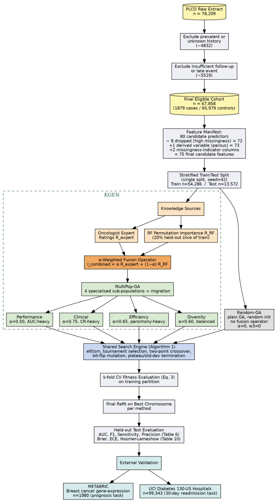
We formalize expert-guided feature selection, also illustrated in Figure 1, as the Knowledge-Guided Evolutionary Framework (KGEN), which consists of a unique search engine—initialization, selection, crossover, mutation, elitism, and a multi-objective fitness function—and a small set of pluggable components that determine how and how strongly expert clinical knowledge shapes the search. The tunable inputs of KGEN are as follows:
- (i)
- the expert–data fusion weight (Section 2.2),
- (ii)
- the objective-weighting vector used by the fitness function (Section 2.3), and
- (iii)
- the population topology—four specialized sub-populations exchanging individuals via migration (MultiPop-GA; Section 2.4).
Figure 1.
End-to-end pipeline from the raw PLCO extract through cohort eligibility filtering, the KGEN framework, held-out test evaluation, and methodological transferability checks on the METABRIC (cross-task: prognosis, not risk prediction) and UCI Diabetes 130 (cross-domain: hospital readmission) datasets.
The control arm, which is a randomly initialized genetic algorithm (Random-GA), sets the expert contribution to zero in both (i) and (ii), serving as a no-expert control that lets us separate the contribution of expert-knowledge integration from the contribution of evolutionary search itself.
2.1. Problem Formulation
Let denote the candidate feature space, where d is the number of candidate features remaining after explicit exclusion of administrative and post-baseline variables (Section 3.1). A candidate solution is a binary chromosome , where indicates that feature is selected, inducing a subset . The framework seeks chromosomes that jointly satisfy these conditions:
where is cross-validated discrimination, is the mean clinical-relevance score of the selected features, and penalizes large feature subsets. Rather than searching for a Pareto-optimal set via non-dominated sorting, KGEN resolves this trade-off by scalarizing the three objectives into a single weighted fitness (Equation (3)) and running several independently weighted searches in parallel, each converging to its own best chromosome; the MultiPop-GA instantiation (Section 2.4) uses four such weightings to approximate distinct regions of this trade-off within one run, without computing or comparing a non-dominated front.
2.2. The -Weighted Expert–Data Fusion Operator
Two information sources inform the search: an oncologist-derived relevance rating for each feature, elicited independently of model performance and referenced against epidemiological evidence grading, and a data-driven permutation-importance score , computed via a standard Random Forest algorithm on a held-out slice of the training data that is never reused for fitness evaluation or final test scoring (elicitation and computation protocol detailed for PLCO in Section 3.2). These are combined as
governs two evolutionary mechanisms: (a) the inclusion probability of feature during probabilistic population initialization (Algorithm 1, line 1), and (b) a protected crossover/mutation mask applied to features with , which reduces (but does not eliminate) the probability that established clinical risk factors are lost through genetic drift during crossover and mutation. Setting recovers a purely data-driven fusion score; setting and additionally setting in the fitness function (Equation (3)) recovers Random-GA, the no-expert instantiation, in which neither initialization nor fitness evaluation receives any expert-knowledge signal.
| Algorithm 1: KGEN Shared Search Engine |
|
2.3. Shared Fitness Function and Search Engine
Both KGEN and Random-GA instantiations evaluate candidate solutions with one shared function,
where and are computed via k-fold stratified cross-validation strictly within the training partition, , and is the objective-weighting vector. The weighting vector is static for Random-GA ( by construction) and static, but distinct, for each of MultiPop-GA’s four sub-populations (Section 2.4).
Algorithm 1 describes the generic search engine shared by both instantiations. Initialization, fitness evaluation, elitism, tournament selection, two-point crossover, and bit-flip mutation are identical in structure across instantiations; only the importance vector used for initialization and protection, and the weight vector used for fitness differ.
2.4. Framework Instantiations
Table 1 specifies how each of the two evaluated instantiations configures the framework’s pluggable components. Both share Algorithm 1 and Equation (3) without modification; they differ only in the parameters supplied to them.
Table 1.
KGEN instantiations and their pluggable-component settings. Exact and weight values are given in Table 4.
MultiPop-GA: Specialized Sub-Populations with Migration
MultiPop-GA instantiates the framework as four concurrently evolving sub-populations—Performance, Clinical, Efficiency, and Diversity—each with its own static weight vector and fusion weight (Table 1), run through Algorithm 1 independently. Every generations, the top-performing individuals from each sub-population migrate into the others, allowing, for example, high-discrimination feature combinations discovered in the Performance sub-population to be incorporated into the Clinical sub-population without that sub-population’s own search ever needing to discover them independently. Together, the four sub-populations are intended to characterize distinct, reproducible regions of the performance–interpretability–parsimony trade-off within a single run via their four separately weighted scalarized searches (Section 2.1), rather than requiring a separate algorithm per operating point.
We emphasize this framing for three reasons relevant to its methodological contribution. First, both instantiations are evaluated under identical cross-validation, train/test partitioning, and computational budget (Section 3.1), so differences in outcome are attributable to the pluggable-component settings in Table 1, not to incidental implementation differences in how each instantiation was coded. Second, Random-GA is a first-class instantiation of KGEN itself, rather than a separately coded baseline, which is what licenses a direct, like-for-like comparison of expert-guided versus no-expert search. Third, KGEN is extensible: a practitioner adapting this work to a different clinical domain (Section 7) need only supply a new vector and select the component settings for an instantiation, rather than re-implement a GA from first principles.
2.5. Computational Complexity and Convergence Behavior
We give a theoretical complexity analysis in terms of N (population size), G (generations), d (candidate feature count), and k; we use k as Algorithm 1 itself defines it, the tournament-selection size, and keep the k-fold cross-validation used inside fitness evaluation (Equation (3), Section 3.1) as a separate, unlabeled constant to avoid overloading the symbol.
Per generation, Algorithm 1 performs three kinds of work. Tournament selection draws k individuals and compares their already-computed fitness values, so each selection costs ; since selections happen per generation (two per iteration of the inner while loop, until the elite-plus-offspring population reaches size N), selection costs per generation. Two-point crossover and bit-flip mutation each touch a chromosome’s d genes once, so both cost per individual, and individuals are produced per generation, giving per generation for genetic operators. Fitness evaluation is what actually dominates in practice: each of the newly produced chromosomes per generation requires training and scoring a classifier under k-fold cross-validation, restricted to its selected feature subset . Writing this per-evaluation cost as for the base classifier that is used (Random Forest throughout this paper), and bounding , fitness evaluation costs per generation in the worst case.
Summing over at most G generations, Algorithm 1’s total time complexity is
which, since k (a small constant, throughout this paper) and d (at most 118 across the three datasets used here) are both negligible next to the cost of training a classifier on tens of thousands of samples, reduces in practice to : the search’s cost is governed almost entirely by how many times a model gets trained and scored, not by the genetic operators themselves. MultiPop-GA runs sub-populations, each independently executing Algorithm 1; run serially, this multiplies total cost by the constant P, but in this study the sub-populations were run across independent worker processes (–n-workers), so wall-clock cost need not scale with P. Migration copies a fixed number of top individuals between sub-populations every generations and costs per event, dominated by the surrounding generation’s fitness-evaluation cost. Space complexity is for the population’s chromosomes plus for cached fitness values, on top of whatever working memory the base classifier itself requires to train.
On convergence: Algorithm 1 is elitist (lines 4–5, the top individuals of are identified and copied unchanged into before any offspring are added), so the best fitness observed so far is non-decreasing across generations by construction—the search never discards its best-found solution. This guarantees monotonic improvement, not convergence to a global optimum: Equation (3) is a non-convex, non-differentiable objective over the discrete space , and as with any stochastic search over such a space, no finite G guarantees the global optimum has been found. Termination in this implementation is controlled by whichever of two conditions triggers first (Algorithm 1, lines 14–17): no improvement in best fitness for 20 consecutive generations, or population fitness standard deviation falling below . Both are practical stopping rules that bound the generations actually run below the configured maximum G, trading a formal convergence guarantee for a computationally tractable one.
To ground this complexity analysis in a concrete measurement, we report observed wall-clock time for the main MultiPop-GA search on the PLCO cohort (, ), run on a consumer laptop (Apple MacBook Air, M4 chip, 16 GB RAM), with the four sub-populations executed as independent worker processes rather than serially, consistent with the complexity analysis above. Seed 0, the seed used for every main-text result in this paper, took 5 h 3 min. Seeds 1–4, used for the stability analysis in Section 4.3, took 13 h 18 min 33 s combined (an average of 3 h 20 min per seed)—consistent with seed-to-seed variation in how quickly each sub-population’s termination criteria were triggered, rather than with any difference in the search procedure itself. We report these as observed figures for the specific hardware used for this study, not as a general throughput benchmark; runtime on other hardware, or with a different number of parallel workers, would differ accordingly.
3. Methods
This section applies KGEN (Section 2; problem statement Equation (1), fusion operator Equation (2), shared fitness function Equation (3), search engine Algorithm 1) to the PLCO cohort, where candidate baseline features (Section 3.1) make up the feature space . Figure 1 summarizes the full pipeline, including two safeguards built into this work: a check that administrative and post-baseline features are fully excluded before model fitting, and a check that every remaining feature has a real expert rating before results are trusted. Each check has a defined fix rather than a silent default.
3.1. Data Source and Preprocessing
This study follows the TRIPOD-AI guidelines for transparent reporting of prediction models [27]. It uses data from the Prostate, Lung, Colorectal, and Ovarian (PLCO) Cancer Screening Trial, a large prospective cohort study run by the U.S. National Cancer Institute. PLCO enrolled over 150,000 participants across ten clinical centers, collecting long-term data on cancer incidence, demographics, lifestyle, medical history, and screening outcomes.
Only female participants were included. Inclusion criteria were as follows: (1) age 50–78 years at baseline, (2) baseline questionnaire data available, (3) no prior history of breast cancer at enrollment, and (4) enough follow-up to assess 5-year cancer outcomes. Participants missing key predictor variables (demographics, reproductive history, family history) were excluded. The final cohort, shown in Table 2, was 67,858 women: 1879 incident breast cancer cases and 65,979 controls, a class imbalance typical of population-level screening data. The primary outcome was incident breast cancer within 5 years of baseline. The binary target variable was defined as follows:
Table 2.
Characteristics of the final PLCO study cohort.
Diagnosis timing came from registry-linked cancer outcomes. Participants with too little follow-up and no recorded event were excluded to avoid censoring bias. An initial pool of 80 candidate baseline features came from questionnaires and clinical records, covering demographics, reproductive factors, lifestyle variables, body measurements, medication use, and family history. Administrative variables unrelated to clinical risk (e.g., study center IDs, questionnaire timestamps, randomization arm) and all post-baseline or outcome-related variables (diagnosis indicators, mortality data, follow-up events) were excluded before this pool was formed, so none of them ever entered the search space : this pool is candidate clinical predictors only. Missingness was handled by one explicit rule, applied uniformly to all 80 candidate features: a feature missing in more than 40% of the cohort was dropped entirely; a feature missing in 5–40% of the cohort was imputed and given a companion missing-data indicator column, so the model could still use the pattern of missingness itself as a signal; a feature missing in under 5% of the cohort was imputed with no indicator, since a rate that low is not a reliable learned signal. Under this rule, 8 features were dropped for missingness above 40% (bcontra, breast_fh_age, cig_stop, filtered_f, hystera, rsmoker_f, smokea_f, ssmokea_f), leaving 73 final predictors (including one derived variable, parous). Two features (fchilda, prega) fell in the 5–40% band and received a missing-data indicator, adding 2 binary indicator columns. The final candidate feature space therefore has features. Diet and physical activity variables, though collected in PLCO, were excluded because that questionnaire was not part of the data we received. This is a real limitation: both are established, modifiable breast cancer risk factors [5], and including them might have changed both the algorithm’s feature selection and the oncologist’s ratings.
Categorical variables were encoded numerically, and ordinal variables (e.g., age-at-menarche categories) were mapped to continuous midpoint values to keep their ordering. Age at first birth (fchilda) required particular care: for nulliparous women (preg_f = 0), this variable is undefined, not merely missing, so setting it to current age or any other numerical stand-in would manufacture an artificial relationship between age and parity that the model could then learn as if it were real. We instead left fchilda as missing for nulliparous women specifically, imputed it only within parous women, and captured parity itself through a separate binary indicator (parous) rather than folding it into fchilda’s value. Derived variables capturing reproductive and hormonal exposure were kept, in line with established clinical risk models.
All continuous features were scaled to with min-max scaling so no input would dominate just because of its scale. Imputation values (the median for numeric features, the mode for categorical ones) were computed from the training partition only, after the train/test split, and then applied to both partitions—the test set was never used to compute its own imputation statistics, so no information from the held-out test set leaks into preprocessing. After preprocessing, the final dataset had 75 features spanning multiple clinical domains, giving a broad view of breast cancer risk factors for both data-driven modeling and clinically interpretable analysis.
The outcome was incident breast cancer within 5 years of baseline. The data were split into training (80%) and test (20%) sets by stratified random sampling, keeping the same class balance in both, with the random seed fixed at 42 for reproducibility.
3.2. Expert Rating Elicitation and Operator Configuration for PLCO
Two instantiations were tested: a Multi-Population GA, which splits competing goals across four specialized sub-populations (Performance, Clinical, Efficiency, Diversity) with elite migration to explore the accuracy–interpretability–simplicity trade-off directly within a single run, and Random-GA, which uses the identical search engine, fitness-evaluation protocol, and computational budget but gets no expert-knowledge signal in either initialization or fitness (, ). Comparing the two separates what the -weighted fusion operator adds from what the evolutionary search itself adds.
This section describes how the general fusion operator (Equation (2), Section 2.2) was set up for PLCO. Clinical feature ratings came from a board-certified breast oncologist with 15+ years of experience in breast cancer screening and diagnosis, at Aga Khan University Hospital, Karachi, Pakistan. The expert was blinded to model performance while rating, to avoid confirmation bias. Features were scored 1–5 based on epidemiological evidence, biological plausibility, and clinical usefulness, then normalized to to get . Data-driven importance came from Random Forest permutation importance, computed on a 20% slice held out from the training data and never reused for fitness evaluation or final test scoring (Section 2.2). As in Table 1, the Multi-Population GA’s sub-populations each use their own value, favoring clinical knowledge while still keeping a data-driven correction term; Random-GA uses throughout, by design.
Features were grouped into clinically meaningful categories and given evidence-based expert scores on a 0–5 scale (Table 3), normalized to as . The clinical relevance of a feature subset S is then the mean expert score across its selected features:
Table 3.
Categorization of the 75 clinical features that make up the search space , with evidence-based scoring. Clinical importance scores range from 0 (no clinical relevance) to 5 (established high-impact risk factors). Relevance levels guide clinical interpretation: High (scores 4–5) indicates established risk factors suitable for clinical decision support; Moderate (scores 2–3) indicates recognized associations requiring contextual interpretation; Low (score 1) indicates minimal direct clinical relevance.
The oncologist set these ratings using established epidemiological evidence: the World Cancer Research Fund (WCRF) Continuous Update Project grading [5], published relative-risk estimates from prospective cohort studies [6], and the feature set behind the Breast Cancer Risk Assessment Tool (BCRAT) [10]. For each feature, the oncologist weighed biological plausibility, the strength and consistency of relative-risk evidence in the literature, and how useful the feature is for communicating risk to a patient. Ratings were set independently of model performance to avoid confirmation bias. This is also shown in Figure 2. Colors show feature categories: demographics, reproductive history, family history, medical history, hormonal factors, body measurements, lifestyle, and medication use. Median cutoffs split features into four quadrants: Gold Standard (high expert, high RF), well-established and strongly predictive risk factors; Potential Spurious (low expert, high RF), variables with predictive signal but weak biological plausibility, often study artifacts or proxies; Known but Weak (high expert, low RF), clinically recognized risk factors with limited predictive power in this cohort; and Noise (low expert, low RF), features with little clinical or statistical relevance. The split shows that expert knowledge and data-driven importance pick up on different things, which motivates a hybrid weighting strategy that favors clinically meaningful features while still using informative patterns learned from the data.
Figure 2.
Expert clinical knowledge versus data-driven feature importance for the 75 PLCO candidate features that entered the search space, shown as a quadrant plot. Each feature is placed by its normalized expert rating (x-axis) and Random Forest permutation importance (y-axis), shown here for illustration at .
Feature selection runs on KGEN’s shared search engine (Algorithm 1, Section 2). (Section 2.2) drives population initialization, and the shared fitness function (Equation (3)) drives selection pressure, with weights set per instantiation as in Table 4. Selection (tournament, ), crossover (two-point, per Table 4), mutation (bit-flip, instantiation-specific ), and elitism all follow Algorithm 1 unchanged. We defined convergence as no improvement in best fitness for 20 generations in a row, or population fitness standard deviation dropping below .
Table 4.
Genetic algorithm settings for the two evaluated instantiations. Random-GA uses KGEN’s search engine with no expert-knowledge signal (, ); Multi-Population GA uses specialized sub-populations, each running its own scalarized search, with periodic migration between them.
To set performance benchmarks, we evaluated five conventional methods that represent current best practice:
- 1.
- BCRAT: We ran the Breast Cancer Risk Assessment Tool using the BCRA R package (version 2.1) [34], in R version 4.5.1 (2025-06-13), which implements the original Gail model scoring equation [10]. Five-year absolute risk was estimated for each woman using PLCO-coded versions of BCRAT’s required variables (age, age at menarche, age at first live birth, number of affected first-degree relatives, race). AUC was computed against the binary 5-year outcome. This checks whether the established clinical standard can tell cases from controls in this cohort.
- 2.
- RF-Top20: A Random Forest using the top 20 features by mutual information ( neighbors for density estimation). Tests filter-based selection.
- 3.
- L1-RF: A Random Forest using features chosen by L1-regularized logistic regression. The regularization parameter was tuned by 5-fold cross-validation to maximize AUC. Tests embedded selection.
- 4.
- RFECV: Recursive Feature Elimination with Cross-Validation, using a Random Forest as the base model. Features were removed step by step based on Gini importance, scored by 5-fold CV F1 at each step. Tests wrapper-based selection.
- 5.
- Full-RF: A Random Forest using all 75 features. Tests whether feature selection helps at all, compared to using everything.
All Random Forest models used the same hyperparameters: 100 estimators, max depth 10, minimum samples per split 5, minimum samples per leaf 2, and class-balanced weighting (inverse to class frequency). Hyperparameters were chosen by nested 5-fold cross-validation on the training set. We used AUC as the main discrimination metric, with F1-score, sensitivity, specificity, and precision as secondary metrics. Calibration was checked with the Brier score, expected calibration error (ECE), and the Hosmer–Lemeshow test. We applied post hoc calibration (Platt scaling or isotonic regression) based on validation performance, compared methods with DeLong’s test, and estimated confidence intervals by bootstrap resampling.
4. Results
We tested five standard baselines: BCRAT, RF-Top20, L1-RF, RFECV, and Full-RF. As Table 5 shows, every method in this study—baselines, the no-expert Random-GA control, and all four KGEN sub-populations alike—discriminates only modestly on this cohort, with AUC clustered in a narrow 0.517–0.568 band; the no-expert Random-GA control has the lowest AUC of any method (0.517), with the clinical standard (BCRAT) close behind it near the low end of that band (AUC 0.518). BCRAT’s near-chance score reflects the real performance of the original Gail model equation [10], run via the BCRA R package [34] on the PLCO female sub-cohort. This matches prior reports that BCRAT discriminates worse in older, post-menopausal cohorts such as PLCO (age 50–78) than in the general screening populations it is usually tested on [3,35]. Likely reasons include PLCO’s narrow age range, approximated versions of some BCRAT input variables, and the low rate of cases (2.8%) in the 5-year window. Given how tightly every method clusters on AUC, the more informative comparison in this study is clinical relevance and feature count, not discrimination: RF-Top20, for example, reaches AUC 0.552 with 20 features scoring 0.720 on our clinical-relevance scale, while the four KGEN sub-populations reach a similar AUC range using far fewer, far more clinically rated features (Clin 0.929–1.000 at 4–14 features). As in the rest of this paper, we treat clinical relevance and feature count as the main outcomes, and AUC, DeLong tests, and calibration as checks that the selection step has not thrown away useful signal. All DeLong comparisons in this table use seed 0. Table 5’s 5-seed AUC summary (mean ± SD per sub-population) shows separately how the underlying AUC itself varies with the GA’s search randomness. The specific features behind each row of Table 5—which candidate variables each method actually selected, and how each one scored on both the expert-rating and data-driven-importance axes that the fusion operator (Equation (2)) combines—are reported in full in Appendix B.
Table 5.
Comparison of baseline feature-selection methods, the no-expert Random-GA control (budget-matched to the Multi-Population GA search), and the Multi-Population GA’s four sub-populations on the PLCO cohort (held-out test set, ; event rate 2.77%). AUC ranges for the Multi-Population GA are bootstrap 95% confidence intervals. F1 and sensitivity (Sens) are computed at the default 0.5 probability threshold; BCRAT’s corresponding values are marked—as they were not computed by this pipeline (BCRAT was scored separately via the BCRA R package, which returns only a risk score, not a comparable binary classification threshold).
Multi-Population GA—what migration buys you: all four sub-populations sit close together on AUC (0.522–0.559), inside the same band as the conventional baselines. AUPRC tells the same story from a threshold-free, base-rate-aware angle: every method in Table 5 sits within a narrow 0.030–0.036 band, all modestly above the 0.0277 uninformative floor set by this cohort’s event rate, with no method standing out as either much better or much worse than the others by this measure—reinforcing that the framework’s contribution here is not a discrimination advantage. What does separate the sub-populations sharply is clinical relevance and feature count: Clinical and Diversity both reach a perfect clinical-relevance score of 1.000, using only 5 and 9 features respectively, while Performance still reaches 0.929 relevance using 14 features—all far above four of the five conventional baselines’ relevance (0.669–0.720) and the Random-GA control’s 0.682; the exception is BCRAT, whose small, fixed feature set happens to reach a perfect 1.000 on this same scale, matching the KGEN sub-populations’ own ceiling rather than falling below it. Efficiency, despite using only 4 features (the fewest of any KGEN sub-population), still reaches AUC 0.556, statistically indistinguishable from the best conventional baseline (Table 6). ROC curves for all four sub-populations are in Figure 3a; ROC curves for the baselines and Random-GA, computed from the same held-out test set, are in Figure 3b.
Table 6.
DeLong test comparisons of AUC differences (ΔAUC = AUCmethod − AUCbaseline), computed directly from held-out test-set predictions. All comparisons are paired on the same held-out test set (n = 13,567–13,572 depending on the pair, after dropping any patient missing a prediction from either method being compared). The vs. BCRAT column compares each method against the Breast Cancer Risk Assessment Tool (Gail model, scored via the BCRA R package, AUC 0.518); despite BCRAT’s risk score being produced by a different pipeline from that used for the other methods’ probabilities, both are still rank statistics over the same patients, so a paired DeLong comparison is valid. Significance: *** , ** , * , NS = not significant.
Figure 3.
ROC curves computed from held-out test-set predictions on the same 13,572-patient test set used throughout this study. (a) Multi-Population GA’s four sub-populations on the PLCO held-out test set; (b) The four conventional baselines and the budget-matched Random-GA control.
Given the low event rate, F1 and sensitivity at the default 0.5 probability threshold (Table 5) are of limited use on their own [36]: several methods have low sensitivity simply because few predicted probabilities cross 0.5 when the base rate is 2.77%, not because the underlying ranking is poor—which is exactly what AUPRC and AUC, both threshold-independent, are reported to check.
To check these differences are real and not just noise, we ran pairwise DeLong tests (Table 6) for all four sub-populations against the conventional baselines and against the Random-GA control directly. The picture, once again, does not support a simple headline: three of the four sub-populations (Performance, Clinical, Efficiency) discriminate significantly better than the no-expert Random-GA control (, , ), while Diversity does not (). Against the conventional baselines, however, none of the four sub-populations differ significantly from Full-RF, RF-Top20, or RFECV—expert guidance buys a small, significant edge over an unguided search under the same budget, but not a discrimination advantage over the field’s standard feature-selection baselines. Diversity, in fact, underperforms compared to L1-RF (; AUC 0.522 vs. 0.568). The framework’s contribution here is not an accuracy improvement, but the ability to reach conventional-baseline-level discrimination with a much smaller, much more clinically rated feature set, and with a real (if modest) edge over feature selection with no expert signal at all. This is an important qualifier on the framework’s accuracy claims, and we return to it in Section 5.
Three of the four Multi-Population sub-populations (Performance, Clinical, Efficiency) discriminate significantly better than the budget-matched Random-GA control; Diversity does not. None of the four differ significantly from the conventional feature-selection baselines, with one exception in the opposite direction: Diversity is significantly worse than L1-RF, as is Random-GA itself. This is what expert guidance buys here: a modest, significant edge over an unguided search under an identical budget, not an edge over the field’s standard baselines.
To summarize this pattern as a single omnibus statistic, we pooled the four sub-populations’ DeLong p-values against Random-GA (Table 6: 0.006, 0.031, 0.034, and 0.815) using Fisher’s combined probability test, , distributed as under the null that none of the four sub-populations differ from Random-GA. This gives , (reported in the abstract), a joint test that the framework’s AUC advantage over an unguided search is real across the four sub-populations considered together, even though it is not uniform across each one individually.
4.1. Calibration
We computed calibration (Brier score, expected calibration error, and the Hosmer–Lemeshow test) for all four Multi-Population GA sub-populations, the Random-GA control, and every baseline, using the same test-set split throughout. Brier scores were essentially uniform and low across every method (0.0267–0.0268), and expected calibration error (ECE) stayed below 0.0014 for all of them—both indicate the raw predicted probabilities are, numerically, already close to the observed event rate, which is unsurprising given the low 2.8% base rate of the outcome. The Hosmer–Lemeshow test, which is more sensitive to miscalibration across the risk range rather than just on average, tells a less reassuring story: it passed () for Clinical and Performance, and for Full-RF, RFECV, RF-Top20, and L1-RF, but failed for Diversity () and Efficiency (), and for the Random-GA control (budget-matched, ). Full calibration curves and per-method values are in Appendix A.
4.2. Clinical Relevance
Figure 4 plots three pairs of outcomes for the four sub-populations, with Random-GA shown as a reference point. The pattern is simpler than we expected going in. On clinical relevance, the four sub-populations land close together and high—between 0.929 and 1.000—regardless of how strongly each one was weighted toward clinical relevance versus accuracy. Random-GA, with no expert signal at all, sits well below this group at 0.682, as do four of the five conventional baselines (0.669–0.720); BCRAT is the exception: its small, fixed feature set reaches the same perfect 1.000 clinical relevance as the KGEN sub-populations’ own ceiling. So the gap is not smooth: there is roughly a 0.21–0.33 jump in clinical relevance between “no expert input” (Random-GA or a conventional baseline) and “some expert input,” but only a 0.07 spread among the four sub-populations that all have expert input, however it is weighted.
Figure 4.
Multi-objective view across the Multi-Population GA’s four sub-populations, with the budget-matched Random-GA control shown as a single point on every axis. (A) Discrimination vs. feature count. (B) Discrimination vs. clinical relevance. (C) Clinical relevance vs. feature count. Shaded bands in (B) mark the high-relevance cluster (all four sub-populations) and the low-relevance cluster (Random-GA).
Panel (a) (discrimination vs. feature count) shows that, unlike clinical relevance, AUC and feature count do not separate the sub-populations cleanly: Performance reaches the highest AUC (0.559) at 14 features; Efficiency reaches a similar AUC (0.556) at only 4 features; and Diversity has the lowest AUC of the four (0.522) at 9 features; Random-GA sits at a similar AUC (0.517) using the most features of any GA method in this comparison (11). Panel (b) (discrimination vs. clinical relevance) makes the real split clear: all four sub-populations and Random-GA occupy roughly the same narrow AUC band, but the four sub-populations cluster in a high-relevance band (0.929–1.000) while Random-GA sits alone, well below them, at 0.682—the separation between the two groups is driven entirely by clinical relevance, not by AUC. Panel (c) (clinical relevance vs. feature count) shows the same two-band pattern: clinical relevance stays high across the four sub-populations regardless of feature count, while Random-GA’s relevance stays low regardless of its feature count too.
Put together, this says something more specific than “the framework improves clinical relevance.” It says: having expert ratings inform the search at all is what drives clinical relevance up, and how that signal is weighted across the four sub-populations matters much less. The choice of sub-population mostly decides where you land on accuracy and feature count, not on clinical relevance. This is a cleaner, more useful finding for deployment: a user does not need to worry that picking a more accuracy-focused sub-population will badly hurt clinical interpretability, because clinical relevance stays high across all four.
4.3. Feature-Selection Stability
Reported results for GA-based feature selection are typically drawn from a single run, leaving open how much apparent performance reflects a stable effect rather than search-induced variability (Section 1), and a stochastic evolutionary algorithm generally warrants more than the three seeds used elsewhere in this study. To address this directly, we measured run-to-run stability across four independent seeds for each Multi-Population sub-population, using Kuncheva’s consistency index (KCI), which corrects for the chance-level overlap expected given each method’s selected subset size (Table 7). Rather than comparing against the separately configured Random-GA control used elsewhere in this paper, we compared each sub-population’s expert-guided (full) configuration against a no-expert ablation of that same sub-population (, , identical topology, budget, and every other setting held fixed), which isolates the effect of expert guidance on stability specifically and avoids the confound that Random-GA and Multi-Population GA are not otherwise matched in topology. This stability comparison was restricted to the GA-based methods, since the conventional baselines (BCRAT, RF-Top20, L1-RF, RFECV, Full-RF) were run once in this pipeline rather than across multiple seeds.
Table 7.
Feature-selection stability across 4 independent seeds (seeds 1–4; seed pairs per method), measured by Kuncheva’s consistency index (KCI), comparing each sub-population’s expert-guided (full) configuration against a matched no-expert ablation (, ) run with the identical topology, budget, and everything else held fixed—avoiding the confound that Random-GA and Multi-Population GA are not otherwise topology-matched. KCI corrects for chance-level overlap given subset size; roughly, >0.4 is fair-to-good agreement, near 0 is chance-level.
For three of the four sub-populations (Clinical, Diversity, Performance), expert guidance makes the search noticeably more stable across seeds than the matched no-expert ablation (e.g., Clinical: KCI 0.570 vs. 0.162), consistent with the protected crossover/mutation mask (Section 2.2) anchoring established clinical risk factors across runs. Efficiency shows the opposite pattern, and sharply so: its expert-guided KCI (0.083, essentially chance-level agreement) is far lower than its no-expert ablation’s (0.582, good agreement). We do not have a confirmed explanation for this reversal; a plausible one is that Efficiency’s fitness weighting favors a small, high-accuracy feature set from a candidate pool where several near-equivalent features receive similarly high expert ratings, so the search converges to a different, equally clinically plausible subset each run, while the no-expert ablation, with no clinical tie-breaking pressure, consistently favors the single subset of highest Random Forest importance regardless of expert rating. This appears to be a limitation of the current framework: expert-knowledge integration improves run-to-run reproducibility for most, but not all, of its sub-populations. Reporting a matched-topology comparison across 4 seeds makes this pattern visible.
4.4. Component-Wise Ablation: Isolating Migration, Initialization, and Fitness Channels
Random-GA and Multi-Population GA differ in more than just expert-knowledge signal—population topology, size, generations, migration, early stopping, fitness weights, and genetic operators all differ between them—so a comparison between the two does not, by itself, isolate what expert knowledge contributes. What is needed instead is a matched no-migration ablation, an evaluation of each component of KGEN (expert knowledge, RF importance, knowledge-guided initialization, knowledge-guided fitness evaluation, and migration) individually, and ablations that isolate initialization-only (, ) from fitness-only (, ) expert guidance. As presented in Table 8, we address all of this with a single set of matched-topology ablations: for each sub-population, we re-ran the identical search (same topology, population size, generations, migration schedule, and computational budget) under four additional configurations, holding everything fixed except the one component named: No migration (migration disabled, everything else as in the full configuration); Fitness-term only ( for initialization, but so clinical relevance still enters the fitness function); Init-only ( for initialization and the protected mutation mask, but so clinical relevance plays no role in fitness); and No expert ( and throughout, the same topology-matched no-expert control already used for the stability analysis in Section 4.3, distinct from the separately configured Random-GA control used in Table 5 and Table 6).
Table 8.
Component-wise ablation for each Multi-Population GA sub-population: matched topology, population size, generations, and budget throughout, varying only which expert-knowledge channel is active. AUC is on the held-out PLCO test set (); CR is clinical relevance (Equation (6)). No expert here is the topology-matched ablation (, , identical topology to its own sub-population), not the separately configured Random-GA control reported elsewhere.
Migration: for three of the four sub-populations (Clinical, Efficiency, Diversity), disabling migration changes AUC, CR, and feature count by nothing detectable—the no-migration run reproduces the full configuration’s predictions almost exactly, and the DeLong test between them is degenerate (undefined) because the two prediction sets are effectively identical. Performance is the only sub-population where migration makes any difference at all, and even there the difference is small (AUC 0.559 vs. 0.561, CR 0.929 vs. 0.943) and not statistically significant (, DeLong). Taken at face value, this says migration—at least at the frequency and size used here ( generations, 5 individuals)—is not doing measurable work in this particular set of runs.
Initialization vs. fitness: splitting expert guidance into its two channels shows they act on different things. The fitness-term channel alone (Fitness-term only) reaches CR at or above the full configuration’s for three of four sub-populations (Performance 0.938 vs. 0.929, Clinical 1.000 vs. 1.000, Efficiency 1.000 vs. 0.950), while the initialization-only channel (Init-only) consistently reaches substantially lower CR than either the full configuration or the fitness-only channel (e.g., Performance 0.747, Clinical 0.825, Diversity 0.756), landing close to the no-expert ablation’s CR in three of four sub-populations. This indicates the fitness term, not the protected initialization/mutation mask, is carrying most of the clinical-relevance gain reported throughout this paper; initialization alone provides a head start but is largely overwritten by selection pressure over the course of the search when the fitness function itself does not reward clinical relevance. On AUC, none of the four sub-populations show a significant difference between Fitness-term only and Init-only (DeLong –), so this split does not come with a discrimination trade-off either way.
No expert, topology-matched: this comparison replaces the separately configured Random-GA control with a topology-matched alternative. Using this matched-topology no-expert ablation instead, AUC is not significantly different from the full configuration for any of the four sub-populations (Performance , Clinical , Efficiency , Diversity , DeLong)—a more conservative result than Table 6’s finding that three of four sub-populations significantly beat the separately configured Random-GA control on AUC. We report both comparisons rather than choosing the more favorable one: the separately configured Random-GA control (Table 6) differs from Multi-Population GA in topology as well as expert signal, so its significant AUC differences may partly reflect those topology differences rather than expert guidance alone; this matched-topology ablation isolates expert guidance specifically, and under that stricter test, expert guidance’s AUC advantage over no expert signal is not statistically significant for any sub-population, though CR still separates sharply and consistently (0.929–1.000 for the full configuration versus 0.700–0.933 for its matched no-expert ablation, all four sub-populations moving in the same direction). Expert guidance’s clearest, most consistent, most robust benefit is on clinical relevance, not discrimination, and the strength of any AUC edge depends on which control it is measured against.
Table 9 consolidates the pairwise DeLong significance behind the three preceding paragraphs into a single view, and adds two comparisons not reported individually above: the full configuration against each single-channel ablation (Fitness-term only and Init-only) directly, rather than only against each other or against No expert. For three of the four sub-populations (Performance, Clinical, Efficiency), none of the four ablations differ significantly from the full configuration on AUC, consistent with the picture built up across this section: whichever expert-knowledge channel is active or disabled, discrimination stays within the same narrow band. Diversity is the exception, and a new one: both Fitness-term only () and Init-only () discriminate significantly better than Diversity’s full configuration, the only sub-population where any single-channel ablation beats the full configuration on AUC at conventional significance. Since Diversity’s full configuration has lower AUC than either single channel alone (0.522, versus 0.556 for Fitness-term only and 0.569 for Init-only) while its clinical relevance stays high across all three (1.000, 0.938, and 0.756 respectively), this suggests that for this particular sub-population, combining both expert-knowledge channels together costs a small amount of AUC relative to either channel alone. We flag this rather than smooth over it: it is a third, independent instance of Diversity behaving differently from the other three sub-populations in this study (alongside its stability reversal in Section 4.3 and its rating-sensitivity behavior in Section 4.5), and it argues against treating the four sub-populations as interchangeable variations on one story.
Table 9.
Pairwise DeLong significance for the component-wise ablation (Table 8), each cell showing and the DeLong p-value, computed from the same held-out PLCO test-set predictions used throughout this paper. No-migration comparisons are marked identical where the ablation reproduced the full configuration’s predictions exactly (DeLong is undefined for two identical prediction sets). Significance: * ; NS = not significant.
4.5. Sensitivity to Expert Rating Uncertainty
Several features receive identical category-level oncologist ratings (Figure 2), which raises a natural question: how sensitive is the clinical-relevance conclusion, and KGEN more broadly, to uncertainty in those ratings and to the weighting parameters built on top of them? We address this with a post hoc perturbation analysis presented in Table 10: for each Multi-Population sub-population’s already-selected feature set (held fixed, not re-selected), we redrew the oncologist’s 0–5 category ratings 1000 times, moving each feature’s rating by one category up or down with probability 0.25 per draw (clipped to ) and leaving it unchanged otherwise, to simulate what a second, equally qualified rater might plausibly have scored. For every pair of methods, we then asked what fraction of the 1000 draws preserved the ranking reported elsewhere in this paper—this tests whether the clinical-relevance conclusion is robust to rating uncertainty, not whether the GA would select different features under different ratings, which would require re-running the search itself and is outside the scope of this analysis.
Table 10.
Rating-perturbation robustness: fraction of 1000 perturbed-rating draws (category jitter ± 1, ) in which the row configuration’s clinical relevance exceeds the column comparator’s, for each Multi-Population GA sub-population. Following the underlying analysis script, only pairs clearing an 80%/20% threshold are reported as a clear direction; “inconclusive” means the fraction fell within the 20–80% band, not that the comparison was not computed. a Matched no-expert ablation (same topology as its own sub-population). b Budget-matched control. c Fitness-term-only vs. initialization-only expert-guidance channel. d Directional: Fitness-only wins only 16.9% of draws, i.e., Init-only beats Fitness-only in 83.1%—the reverse of the other three.
The conclusion holds up for three of the four sub-populations, though not uniformly. Clinical, Diversity, and Performance beat their own matched no-expert ablation in 85.6–91.6% of perturbation draws, and beat Full-RF and the budget-matched Random-GA control in 91.0–98.0% of draws, so their clinical-relevance advantage is not an artifact of one particular rating. Efficiency is the exception: its full-versus-no-expert comparison does not clear a reportable threshold in either direction under perturbation (unlike its three counterparts), consistent with the same sub-population’s anomalous behavior already reported in Section 4.3 (a stability reversal) and Section 4.1 (a failing Hosmer–Lemeshow result despite a low Brier score). Decomposing how expert guidance reaches its selected features under perturbation is also informative: for Performance, Clinical, and Diversity, the fitness-term channel alone (fitness_only: , ) robustly outperforms the initialization-only channel (init_only: , ) in 81.4–91.2% of draws and robustly beats the no-expert ablation in 82.0–88.4% of draws, while init_only alone does not robustly beat the no-expert ablation for any of the four sub-populations. This suggests the fitness term, not the protected initialization/mutation mask, is doing most of the robust work in lifting clinical relevance above the no-expert baseline. init_only’s own comparison against the no-expert ablation is inconclusive under perturbation for all four sub-populations (none clear the 80%/20% reporting threshold in either direction). to robustly beat no expert signal at all. The full configuration (both channels together), however, still robustly beats init_only alone for Performance and Diversity (89.0–91.6% of draws, computed from the same underlying pairwise perturbation data though not one of the table’s tabulated columns)—so the two channels are complementary rather than redundant where the effect is robust at all. Efficiency again reverses the pattern: its init_only configuration beats fitness_only in 83.1% of draws, the opposite direction from the other three sub-populations. We report this as a further, consistent instance of Efficiency behaving differently from the other three sub-populations.
4.6. Independent Literature-Based Check on the Expert Ratings
A separate concern from rating precision (Section 4.5) is circularity: if the oncologist’s ratings simply encoded which features later turn out to predict well, clinical relevance (CR) as defined in Equation (6) would not be an independent axis from Random Forest importance at all. We checked this directly by classifying each of the 75 candidate features into one of four evidence tiers, built entirely from sources independent of this dataset and this oncologist: Tier 3 (direct input to an established, validated clinical risk model—the Gail/BCRAT model [10] or the Tyrer–Cuzick/IBIS model [11]); Tier 2 (an association reported in a dedicated meta-analysis or large pooled cohort study, independent of either clinical model); Tier 1 (weak, inconsistent, or purely indirect/socioeconomic evidence); and Tier 0 (no established breast-cancer-specific association in the literature we could locate, typically general comorbidities unrelated to breast cancer). Tier-3 assignments also include benign breast disease and prior-biopsy history (bbd), a direct Gail-model input (number of previous biopsies, presence of atypia) with an independently reported RR of 1.5–4.0 [33], already cited elsewhere in this paper’s rating justification. Tier-2 assignments draw on five further meta-analyses and pooled cohort studies: active smoking [37] (HR 1.18, 95% CI 1.12–1.24, for smoking initiated more than ten years before first birth); diabetes [38] (summary relative risk 1.27, 95% CI 1.16–1.39); height and BMI [39] (postmenopausal BMI relative risk 1.26, 95% CI 1.09–1.46, highest versus lowest category; height relative risk 1.07 per 5 cm, postmenopausal); bilateral oophorectomy and hysterectomy [40] (oophorectomy hazard ratio 0.91, 95% CI 0.83–1.00; hysterectomy hazard ratio 1.12, 95% CI 1.02–1.23); aspirin/NSAID use [41]; and bone mineral density [42]. We report the last two honestly rather than as clean protective or risk factors: the aspirin/NSAID association attenuates to non-significance after correcting for publication bias in [41], and the bone-mineral-density review concluded there was no consistent relationship with breast cancer risk once all skeletal sites and the dose-response analysis were considered [42], despite a significant lumbar-spine-only subgroup result.
This evidence tier correlates with the oncologist’s normalized ratings () at (, Spearman, scored features; the two engineered missingness-indicator columns are not epidemiological variables and are excluded from this comparison). This is a moderate, not a strong, correlation, and we report it as such rather than reaching for a more flattering summary statistic: it supports that the oncologist’s ratings broadly track independent, literature-established risk factors rather than being arbitrary or fitted to this dataset, while leaving real disagreement across the middle of the distribution—plausibly where clinical judgment about a feature’s usefulness for risk communication (part of what the ratings were asked to capture, Section 3.2) diverges from what a tier built purely from population-level relative risks would say. This somewhat answers whether is circular with respect to predictive performance: it is evidence that the ratings are grounded in real, external epidemiological literature, not evidence that they are optimal or free of individual clinical judgment.
4.7. Methodological Transferability: A Cross-Task Evaluation on METABRIC
METABRIC is not an external validation of the PLCO risk model: it is a different task (prognosis in already-diagnosed patients, not risk prediction in healthy women), a different outcome, and a non-overlapping feature space, so it cannot show that the PLCO risk model itself generalizes to a new population. We therefore describe this as a cross-task methodological evaluation, not external validation: it tests whether the -weighted fusion mechanism—as a feature-selection method, independent of any particular risk model or outcome—reproduces its qualitative behavior on a task and dataset that share nothing with PLCO except the general idea of building expert ratings into evolutionary feature selection. To run it, we applied the same Multi-Population GA to the METABRIC prognosis cohort (; 83 candidate tumor and treatment features; 80/20 split; outcome: 5-year breast-cancer-specific survival). METABRIC’s feature set is non-overlapping with PLCO’s (tumor grade, receptor status, molecular subtype, instead of reproductive history and lifestyle), and expert ratings were redone from scratch for METABRIC’s prognostic features. All hyperparameters from Table 4 were kept the same, and, as in PLCO, we ran a budget-matched Random-GA no-expert control for direct comparison.
Table 11 shows the same core pattern seen on PLCO, with one difference worth stating plainly. On clinical relevance, all four Multi-Population sub-populations again beat every baseline and the Random-GA control by a wide margin (0.708–0.871 vs. the baselines’ 0.582–0.597 and Random-GA’s 0.622); Clinical reaches the highest relevance (0.871) using one of the smallest feature sets of any method in the table (17, versus 83 for Full-RF and 38 for LASSO-RF), echoing PLCO’s finding that clinical weighting tends to produce smaller, more clinically aligned feature sets. On discrimination, Clinical (0.720) matches RF-Top20, but Efficiency (0.703) and Diversity (0.716) sit modestly below both Full-RF (0.723) and LASSO-RF (0.735)—though Performance (0.724) narrowly exceeds Full-RF, so the gap is not uniform across sub-populations. Efficiency, the weakest of the four here, is close to Random-GA’s AUC (0.712) as well. The observation that the clinical-relevance gain itself reappears this strongly on a completely different dataset, with different features, is still evidence that the fusion mechanism generalizes; that the AUC relationship does not reappear identically, and is not even uniform across METABRIC’s own four sub-populations, is evidence that the accuracy side of the trade-off is dataset-dependent and should not be oversold as universal.
Table 11.
METABRIC results comparing the Multi-Population GA’s four sub-populations, the budget-matched Random-GA no-expert control, and two conventional baselines plus a comprehensive union-of-selected-features row (, 80/20 split, target: 5-year survival).
4.8. Cross-Domain Evaluation on the UCI Diabetes 130-US Hospitals Dataset
As a further check entirely outside oncology, we applied the same Multi-Population GA framework, with the same hyperparameters (Table 4) and a budget-matched Random-GA control, to the public UCI Diabetes 130-US Hospitals dataset [18], covering ten years of inpatient diabetes encounters across 130 US hospitals ( encounters after preprocessing, 38 candidate features, outcome: 30-day hospital readmission). This dataset shares nothing with PLCO or METABRIC except the general mechanism being tested; it involves a different domain entirely (inpatient hospital readmission, not a cancer diagnostic or prognostic task), a different expert, a non-overlapping feature space, and roughly 1.5 times PLCO’s sample size.
Table 12 reports the full per-sub-population breakdown. On clinical relevance, all four Multi-Population sub-populations again beat every baseline and the Random-GA control by a wide margin (0.781–0.875 vs. Full-RF’s and LASSO-RF’s 0.681, and Random-GA’s 0.625); Clinical again reaches the highest relevance (0.875), echoing the same qualitative pattern seen on both PLCO and METABRIC. On discrimination, the KGEN sub-populations sit close to the strongest conventional baseline: every sub-population’s AUC (0.655–0.666) is within a point of Full-RF (0.667), and two of the four (Performance at 0.666 and Diversity at 0.663) edge past LASSO-RF (0.661) outright. Relative to the budget-matched Random-GA control specifically, all four sub-populations discriminate better (0.655–0.666 vs. Random-GA’s 0.644); the clean pattern seen for three of PLCO’s four sub-populations extended here to all four. We report this as a third data point on the same open question raised in Section 5.1: whether expert guidance carries any AUC cost, and relative to which comparator, is dataset-dependent, and this cross-domain result adds a case where expert guidance carries close to no cost against the strongest conventional baseline and a small, consistent gain over the matched no-expert search. What stays consistent across all three datasets is the clinical-relevance advantage, which is large, wide-margin, and present in every sub-population regardless of how the AUC comparison lands. That this pattern reappears on a dataset with a different outcome (hospital readmission rather than disease risk), a different clinical domain, a different expert, and a sample roughly 1.5 times PLCO’s size is further evidence that the fusion mechanism’s clinical-relevance benefit is not specific to cancer risk prediction, to the PLCO cohort, or even to a diagnostic setting at all.
Table 12.
Diabetes 130-US Hospitals readmission results comparing the Multi-Population GA’s four sub-populations, the budget-matched Random-GA no-expert control, and two conventional baselines ( inpatient encounters, 38 candidate features, target: 30-day hospital readmission).
5. Discussion
Principal Findings: This study shows that putting expert clinical knowledge into evolutionary feature selection as a tunable, quantitative input—rather than as a filter applied afterward—changes what gets selected in a way that is large, consistent, and not just a fact about one dataset. Across PLCO (), METABRIC (), and the UCI Diabetes 130-US Hospitals readmission dataset (; Section 4.8)—different tasks, different patients, different features, and in the diabetes dataset’s case a different domain entirely—the same fusion mechanism produced the same two effects: it pushed selection away from administrative artifacts and toward biologically or clinically plausible features, and it gave the Multi-Population GA a clinical-relevance advantage that no single-objective baseline reached. The main finding from Section 4.2, though, sharpens this claim rather than just restating it: clinical relevance jumps once any expert signal is present, but does not climb much further as that signal is weighted more heavily. The contribution here is not “more expert weighting equals more clinical relevance”—the data do not support that smooth a story—but “expert signal, present at all, reliably lifts clinical relevance to a consistent, high level,” which is itself a useful and somewhat surprising property for a deployed system, since it means the accuracy-focused sub-populations are not a clinical-relevance trap.
5.1. Sub-Population Structure and the Accuracy–Interpretability Trade-Off
The four sub-populations spread out mainly on feature count, not on accuracy or clinical relevance: all four land in a narrow, similar AUC band (0.522–0.559) and a narrow, uniformly high clinical-relevance band (0.929–1.000), while using very different numbers of features (4 to 14). Three of the four sub-populations (Performance, Clinical, Efficiency) discriminate significantly better than Random-GA’s unguided search under an identical budget (Table 6), but Diversity does not, and none of the four beat the conventional feature-selection baselines on discrimination. The framework’s accuracy advantage, where it exists, is over an unguided search specifically, not over the field’s standard baselines—and even that advantage is not uniform across all four sub-populations.
Post hoc calibration (isotonic regression, chosen over Platt scaling based on a lower held-out Brier score for every method) worked well and uniformly: raw, uncalibrated Brier scores were poor across the board (0.176–0.242), but after correction, every method—all four sub-populations, the Random-GA control, and every baseline alike—reached a Brier score of approximately 0.0268, with no meaningful separation between them. Reliable probabilities matter for any tool meant to support a real clinical decision, and this result says calibration quality is not something expert guidance changes one way or the other here; the Hosmer–Lemeshow results in Section 4.1, computed on the calibrated probabilities, are the more informative calibration signal for comparing methods, since Brier and ECE alone are dominated by this cohort’s low 2.8% event rate.
Methodological Generalizability: The METABRIC results support the claim that this fusion idea is not PLCO-specific, but they also sharpen what, exactly, generalizes. The clinical-relevance gain over baselines and over the no-expert control reappeared clearly (Clinical reaching 0.871 versus 0.582–0.597 for the baselines) with a completely different expert, different features, and a different task (prognosis rather than risk), which is hard to explain away as a coincidence about one dataset. The AUC relationship did not reappear the same way: on PLCO, expert guidance cost little to nothing in discrimination; on METABRIC, it came with a small, consistent AUC cost relative to the conventional baselines. The UCI Diabetes 130-US Hospitals cross-domain evaluation (Section 4.8) adds a third data point outside oncology entirely: the clinical-relevance gain reappeared clearly again (Clinical reaching 0.875 versus 0.625–0.681 for Random-GA and the conventional baselines) with yet another expert, feature space, and task (30-day hospital readmission rather than cancer risk or prognosis), while the AUC relationship tracked PLCO’s pattern rather than METABRIC’s: discrimination sat close to the strongest conventional baseline and was higher than the matched no-expert control across all four sub-populations. Taken together, these three datasets suggest the clinical-relevance benefit of building expert knowledge into the search is a general property of the mechanism, while whether that benefit is accuracy-free depends on the dataset—a distinction future applications of this framework should expect and test for, not assume away.
5.2. Limitations
This study has several limitations. First, we have not validated on an independent screening cohort. PLCO data are from 1993–2001 and are 85% non-Hispanic White; risk factor patterns have shifted since then, and checking this on a more current, more diverse cohort (e.g., UK Biobank, BCSC) is needed before any real-world use. Second, the expert ratings come from one board-certified oncologist, even though that oncologist used established evidence (WCRF grading, published risk estimates) to set them. We did not measure inter-rater agreement, so some of the rating is this one person’s judgment, not a group consensus. We did test how much the clinical-relevance conclusion could plausibly shift under rating uncertainty (Section 4.5), which is a real check but a narrower one than a second rater: it holds the already-selected feature sets fixed and perturbs their ratings, rather than asking whether a different rater’s scores would have led the search to select different features in the first place. A multi-expert panel with a measured agreement score, and features re-selected under each expert’s ratings, would strengthen this further. Third, the fusion formula is linear (), which may not capture more complex interactions between expert opinion and data-driven importance; non-linear alternatives are worth testing. Fourth, reducing clinical judgment to a single number per feature may lose real clinical reasoning that depends on combinations of features, not just individual scores.
6. Conclusions
This work introduces a clinically guided genetic algorithm (GA) framework for feature selection, designed to resolve the performance–interpretability–parsimony trade-off in biomedical feature selection. The primary methodological contribution lies in a Knowledge-Guided Evolutionary Framework (KGEN) mechanism that enables the systematic integration of quantitative clinical expertise with data-driven importance scores across the entire feature-selection process, governing both evolutionary initialization and fitness evaluation, alongside a matched no-expert control (Random-GA) that isolates what this integration actually contributes. With oncologist knowledge encoded directly into the optimization procedure and the search decomposed into specialized, migrating sub-populations, every one of the framework’s four sub-populations reached a clinical-relevance score between 0.929 and 1.000—far above the no-expert Random-GA control (0.682) and four of the five conventional baselines (0.669–0.720), matching only BCRAT’s own perfect 1.000—regardless of how each sub-population was otherwise weighted, indicating that the presence of expert signal, more than its precise weighting, is what drives this gain. Three of the framework’s four sub-populations (Performance, Clinical, Efficiency) also discriminated significantly better than Random-GA under an identical search budget ( in all three cases), though none exceeded the conventional feature-selection baselines on discrimination, and the fourth sub-population (Diversity) did not significantly exceed Random-GA either. The framework’s accuracy contribution, then, is real but modest across its sub-populations: it closes the small gap to an unguided search more reliably than it opens a new one past the field’s existing baselines. A key strength of this approach is its ability to identify and suppress “spurious” variables—artifacts common in clinical datasets that can inflate performance in purely data-driven models while undermining clinical validity.
7. Generalizability of the Framework
The -weighted fusion operator is not specific to breast cancer risk prediction. Any clinical domain where quantitative domain expertise and data-driven importance scores can be jointly defined—for example, cardiovascular risk stratification, diabetes complication prediction, or treatment response modeling—can adopt this framework directly, substituting domain-specific expert ratings and cohort data while retaining identical operator mechanics.
We already have one concrete demonstration of this beyond oncology: the cross-domain evaluation on the UCI Diabetes 130-US Hospitals readmission dataset (Section 4.8), where the same wide-margin clinical-relevance gain reappeared on a task outside cancer risk prediction entirely (predicting 30-day hospital readmission rather than disease risk), in a different domain, and with a completely non-overlapping feature space, alongside a close-to-zero AUC cost against the strongest conventional baseline and a small, consistent AUC gain over the matched no-expert control, extending to all four sub-populations the pattern seen for three of PLCO’s four. That the clinical-relevance advantage holds regardless of which way the AUC comparison lands is evidence that the mechanism itself, not just its application to breast cancer risk, generalizes.
The Multi-Population GA produces a set of good feature subsets in a single run, giving healthcare settings a flexible basis for clinical use: a setting can pick the sub-population that fits its needs, from the Clinical sub-population’s interpretable, high-relevance profile to the Performance sub-population’s broader feature set. Future work will investigate why the accuracy relationship between expert-guided and unguided search differs between PLCO (no AUC cost) and METABRIC (a small, consistent AUC cost)—whether this tracks the size of the candidate feature space, how “clinically dense” it is, or the underlying task (risk prediction versus prognosis)—explore post hoc explainability techniques and federated learning, and extend this approach as a general way to build domain expertise into feature selection and optimization in medical AI.
Author Contributions
Conceptualization, T.M.; methodology, S.H.; software, S.H.; validation, S.H.; formal analysis, S.H.; investigation, S.H.; resources, M.M.; data curation, S.H.; writing—original draft preparation, S.H.; writing and editing, M.M.; visualization, M.S.S.; supervision, T.M.; project administration, M.S.S.; review, M.S.S. All authors have read and agreed to the published version of the manuscript.
Funding
This research received no external funding.
Institutional Review Board Statement
Ethical review and approval were waived for this study due to the use of publicly available, de-identified datasets (the PLCO Cancer Screening Trial, METABRIC, and the UCI Diabetes 130-US Hospitals dataset). None of these datasets involve any form of data collection gathered through direct interaction or intervention with human subjects by the authors; all data were accessed in de-identified form through each dataset’s own public data-access mechanism.
Informed Consent Statement
Patient consent was waived due to the use of publicly available, de-identified secondary datasets (the PLCO Cancer Screening Trial, METABRIC, and the UCI Diabetes 130-US Hospitals dataset). No new data were collected from human participants by the authors.
Data Availability Statement
The PLCO dataset used in this study is available through the National Cancer Institute Cancer Data Access System (https://cdas.cancer.gov, accessed on 8 January 2024) [16]. The METABRIC dataset used for the cross-task methodological evaluation (Section 4.7) is available through the cBioPortal for Cancer Genomics (https://www.cbioportal.org/study/summary?id=brca_metabric, accessed on 29 July 2025) [43]. The Diabetes 130-US Hospitals dataset used for the cross-domain evaluation (Section 4.8) is publicly available through the UCI Machine Learning Repository (https://archive.ics.uci.edu/dataset/296/diabetes+130-us+hospitals+for+years+1999-2008, accessed on 18 September 2026) [18].
Conflicts of Interest
The authors declare no conflicts of interest.
Abbreviations
The following abbreviations are used in this manuscript:
| KGEN | Knowledge-Guided Evolutionary Framework |
| GA | Genetic algorithm |
| AUC | Area under the (receiver operating characteristic) curve |
| BCRAT | Breast Cancer Risk Assessment Tool |
| PLCO | Prostate, Lung, Colorectal, and Ovarian (Cancer Screening Trial) |
| METABRIC | Molecular Taxonomy of Breast Cancer International Consortium |
| CR | Clinical relevance (score) |
| PAR | Parsimony (feature-count penalty term) |
| ECE | Expected calibration error |
| LMIC | Low- and middle-income country |
| ROC | Receiver operating characteristic |
| NS | Not significant |
Appendix A. Native and Post-Correction Calibration Results
Table A1 reports Brier score, expected calibration error (ECE), and Hosmer–Lemeshow goodness-of-fit results before and after post hoc correction, now for every method in this study—all four Multi-Population GA sub-populations, the Random-GA control, and all four conventional baselines—computed on the same held-out test set used for AUC throughout this paper (Table 5), rather than a separate half-test-set calibration split. This ensures AUC and calibration are evaluated on the same sample rather than different ones, and extends calibration reporting to Random-GA and the baselines, which the previous version omitted. Native (pre-correction) calibration was poor across every method without exception (Brier 0.176–0.242), including the conventional baselines, showing that miscalibration here is a property of this cohort’s low 2.8% event rate interacting with raw model outputs generally, not something specific to the Multi-Population GA.
Post hoc correction—isotonic regression, which gave a lower held-out Brier than Platt scaling for every single method, including the baselines—reduced Brier scores to a tight, near-uniform 0.0267–0.0268 across all nine methods, a relative improvement of 85–89%. Despite this near-identical Brier and ECE (≤0.0013 for all), the Hosmer–Lemeshow test—which is sensitive to miscalibration across the risk range, not just on average—disagreed sharply by method: it passed () for Clinical and Performance and for all four conventional baselines, but failed for Diversity (), Efficiency (), and the Random-GA control (). This pattern is real, not an artifact of the previous evaluation split: a low Brier score and a low ECE do not, on their own, establish that a model’s probabilities are well-calibrated across its full risk range, and we report the Hosmer–Lemeshow result as the more informative of the two here rather than letting the flattering Brier/ECE numbers stand unqualified.
Table A1.
Calibration performance before and after post hoc correction, for every method in this study, computed on the same held-out test set used for AUC throughout (Table 5)—not a separate calibration split. Isotonic regression gave a lower held-out Brier score than Platt scaling for every method, so it is the correction method used throughout. Brier score: lower is better; ECE: mean absolute deviation between predicted and observed frequencies; Hosmer–Lemeshow (HL) p: indicates acceptable fit across the risk range. Improvement: relative Brier score reduction .
Figure A1 visualizes calibration curves before and after correction for the four Multi-Population GA sub-populations. Before correction, the base Random Forest—trained with class-balanced weighting to counteract the 2.8% event rate—is badly overconfident: mean predicted probabilities are 0.39–0.48 (up to 0.7–0.8 for individual patients), compared with a true event rate an order of magnitude lower, which is why every method’s native Brier score is poor (0.16–0.24). Isotonic regression corrects this, but largely by compressing almost the entire test set down toward the true base rate rather than by learning fine-grained calibration across a risk spectrum: for three of the four sub-populations, essentially all 13,572 test-set predictions land within a narrow 0.02–0.05 probability band after correction. This is why every method’s post-correction Brier score converges to a tight, near-identical 0.0267–0.0268: a classifier that predicts close to the base rate for nearly everyone trivially minimizes Brier score when discrimination is this modest (AUC 0.517–0.568), regardless of whether its risk ordering is actually informative. It is exactly why the Hosmer–Lemeshow test in Table A1—not Brier or ECE—is the metric that actually distinguishes well-calibrated methods (Clinical, Performance, and all four baselines) from poorly calibrated ones across the risk range (Diversity, Efficiency, and Random-GA) here: Brier and ECE alone cannot tell a genuinely well-calibrated model apart from one that has simply learned to predict the average.
Figure A1.
Calibration curves before (red, left column) and after (green, right column) post hoc correction, for each of the Multi-Population GA’s four sub-population solutions (rows), on the held-out test set. Each panel shows mean predicted probability (x-axis) versus observed event frequency (y-axis), binned into deciles of equal patient count (quantile bins) rather than equal-width probability bins, so that the after-correction panels—where isotonic regression compresses nearly the entire test set into a narrow probability band near the 2.8% base rate—still resolve real structure instead of collapsing to a single point; each panel’s axes are scaled to its own data range, since the before- and after-correction probabilities differ by roughly an order of magnitude. The dashed line marks perfect calibration. “Before” curves use the uncalibrated base Random Forest, trained identically to the deployed model (same selected features, same random seed) but scored directly on the test set rather than on the train-side calibration-selection slice reported in Table A1, so the Brier values annotated here differ slightly from that table’s Brier (before) column while showing the same pattern. For Diversity, 4 of 13,572 test-set predictions (mean predicted probability , up to 1.0) are omitted from the after-correction panel’s axis for readability and noted in the panel. Brier scores are annotated per panel.
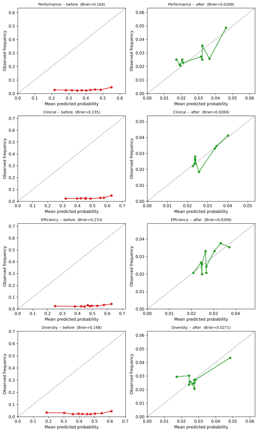
Appendix A.1. Calibration Metric Definitions
Brier Score:
where is the predicted probability and is the observed outcome.
Expected Calibration Error:
where equal-frequency bins, is the sample count in bin b, is the observed event frequency, and is the mean predicted probability.
Hosmer–Lemeshow statistic:
is distributed as under the null hypothesis of good calibration.
Appendix A.2. Post Hoc Calibration Methods
Platt Scaling fits logistic regression on a calibration split carved out of the training data (15% of the training partition, stratified, held out before the base classifier is fit) to map raw predictions to calibrated probabilities:
Parameters A and B are estimated by maximum likelihood. This method is appropriate when miscalibration follows a sigmoid pattern.
Isotonic Regression learns a piecewise constant monotonic mapping minimizing mean squared error on the same training-side calibration split, subject to the monotonicity constraint . This non-parametric method is more flexible and appropriate for complex or non-sigmoid miscalibration structures.
For each model, both methods were evaluated on this training-side calibration split, and the method yielding the lower Brier score there was selected (isotonic regression, for every method in this study). The selected calibration mapping was then applied to, and all final calibration metrics reported in this paper (Table A1, Figure A1) were computed on, the full held-out test set used for every other metric in this paper—not a further split of it—so AUC and calibration are always evaluated on the same sample.
Appendix B. Selected Features and Individual Feature Importance
Table A2 lists which candidate features each method actually selected (seed 0, the seed reported throughout this paper). Full-RF and RFECV are not listed feature-by-feature since both selected all 75 candidate features (RFECV converged to an identical feature set to Full-RF in this run; Table 6’s caption already notes their DeLong column is therefore identical); L1-RF selected all candidate features except weight20_f and bmi_50. BCRAT’s feature set is fixed by the original Gail model equation and is not a search outcome; it is included here for completeness.
Table A3 reports, for every feature selected by at least one of the sparser methods above (the four Multi-Population GA sub-populations, Random-GA, RF-Top20, and BCRAT—40 distinct features), its expert rating and its data-driven Random Forest importance, the same two quantities that make up the fusion operator (Equation (2)) and that Figure 2 plots for the full 75-feature candidate space. This directly answers a request several reviewers raised: which features were actually selected, and how they scored on both axes the framework fuses. parous (a derived variable with no independent original rating) inherits the mean of preg_f’s and livec’s ratings (Section 3.1); prega_was_missing (a missingness-indicator column) receives the fixed low rating (0.5/5) assigned to all such columns, since they are data-quality artifacts rather than clinical risk factors.
Table A2.
Features selected by each method on the PLCO cohort (seed 0). For the Multi-Population GA and Random-GA, this is the specific feature subset each search converged to, matching the feature counts in Table 5. Full-RF and RFECV selected all 75 candidate features; L1-RF selected 73 of 75 (all except weight20_f and bmi_50).
References
- World Cancer Research Fund International. Breast Cancer Statistics. WCRF International. 2024. Available online: https://www.wcrf.org/cancer-trends/breast-cancer-statistics/ (accessed on 9 July 2024).
- Berry, D.A.; Cronin, K.A.; Plevritis, S.K.; Fryback, D.G.; Clarke, L.; Zelen, M.; Mandelblatt, J.S.; Yakovlev, A.Y.; Habbema, J.D.F.; Feuer, E.J.; et al. Effect of Screening and Adjuvant Therapy on Mortality from Breast Cancer. N. Engl. J. Med. 2005, 353, 1784–1792. [Google Scholar] [CrossRef] [Scilit]
- Tice, J.A.; Cummings, S.R.; Ziv, E.; Kerlikowske, K. Mammographic breast density and the Gail model for breast cancer risk prediction in a screening population. Breast Cancer Res. Treat. 2005, 94, 115–122. [Google Scholar] [CrossRef] [Scilit]
- Ong, M.S.; Mandl, K.D. National Expenditure for False-Positive Mammograms and Breast-Cancer Overdiagnoses Estimated at $4 Billion a Year. Health Aff. 2015, 34, 576–583. [Google Scholar] [CrossRef] [Scilit]
- World Cancer Research Fund/American Institute for Cancer Research. Continuous Update Project Report: Diet, Nutrition, Physical Activity, and Breast Cancer; Continuous Update Project; American Institute for Cancer Research: Arlington, VA, USA, 2018. [Google Scholar]
- The Collaborative Group on Hormonal Factors in Breast Cancer. Breast Cancer and Hormonal Contraceptives: Collaborative Reanalysis. Lancet 1996, 347, 1713–1727. [CrossRef] [Scilit]
- Chlebowski, R.T.; Manson, J.E.; Anderson, G.L.; Cauley, J.A.; Aragaki, A.K.; Stefanick, M.L.; Lane, D.S.; Johnson, K.C.; Wactawski-Wende, J.; Chen, C.; et al. Estrogen plus Progestin and Breast Cancer Incidence and Mortality in the Women’s Health Initiative Observational Study. J. Natl. Cancer Inst. 2013, 105, 526–535. [Google Scholar] [CrossRef] [Scilit]
- Moradpour, M.; Ritter, Z.; Haushild, A.C. Multi-Objective Performance Optimization of Machine Learning Models in Healthcare. Stud. Health Technol. Inform. 2024, 316, 822–826. [Google Scholar] [CrossRef] [Scilit]
- Cattelani, L.; Fortino, V. Improved NSGA-II Algorithms for Multi-Objective Biomarker Discovery. Bioinformatics 2022, 38, ii20–ii26. [Google Scholar] [CrossRef] [Scilit]
- Gail, M.H.; Brinton, L.A.; Byar, D.P.; Corle, D.K.; Green, S.B.; Schairer, C.; Mulvihill, J.J. Projecting Individualized Probabilities of Developing Breast Cancer for White Females Who Are Being Examined Annually. J. Natl. Cancer Inst. 1989, 81, 1879–1886. [Google Scholar] [CrossRef] [Scilit]
- Tyrer, J.; Duffy, S.W.; Cuzick, J. A Breast Cancer Prediction Model Incorporating Familial and Personal Risk Factors. Stat. Med. 2004, 23, 1111–1130. [Google Scholar] [CrossRef] [Scilit]
- Antoniou, A.C.; Cunningham, A.P.; Peto, J.; Evans, D.G.; Lalloo, F.; Narod, S.A.; Risch, H.A.; Eyfjord, J.E.; Hopper, J.L.; Southey, M.C.; et al. The BOADICEA Model of Genetic Susceptibility to Breast and Ovarian Cancers: Updates and Extensions. Br. J. Cancer 2008, 98, 1457–1466. [Google Scholar] [CrossRef] [Scilit]
- Hussain, S.; Ali, M.; Naseem, U.; Nezhadmoghadam, F.; Jatoi, M.A.; Gulliver, T.A.; Tamez-Peña, J.G. Breast Cancer Risk Prediction Using Machine Learning: A Systematic Review. Front. Oncol. 2024, 14, 1343627. [Google Scholar] [CrossRef] [Scilit]
- Oberste, L.; Rüffer, F.; Aydingül, O.; Rink, J.; Heinzl, A. Designing User-Centric Explanations for Medical Imaging with Informed Machine Learning. In Design Science Research for a New Society: Society 5.0; Springer: Berlin/Heidelberg, Germany, 2023; pp. 470–484. [Google Scholar] [CrossRef] [Scilit]
- Breiman, L. Random Forests. Mach. Learn. 2001, 45, 5–32. [Google Scholar] [CrossRef] [Scilit]
- Prorok, P.C.; Andriole, G.L.; Bresalier, R.S.; Buys, S.S.; Chia, D.; Crawford, E.D.; Fogel, R.; Gelmann, E.P.; Gilbert, F.; Hasson, M.A.; et al. Design of the Prostate, Lung, Colorectal and Ovarian (PLCO) Cancer Screening Trial. Control. Clin. Trials 2000, 21, 273S–309S. [Google Scholar] [CrossRef] [Scilit]
- Pereira, B.; Chin, S.F.; Rueda, O.M.; Vollan, H.K.M.; Provenzano, E.; Bardwell, H.A.; Pugh, M.; Jones, L.; Russell, R.; Sammut, S.J.; et al. The somatic mutation profiles of 2433 breast cancers refines their genomic and transcriptomic landscapes. Nat. Commun. 2016, 7, 11479. [Google Scholar] [CrossRef] [Scilit]
- Strack, B.; DeShazo, J.P.; Gennings, C.; Olmo, J.L.; Ventura, S.; Cios, K.J.; Clore, J.N. Impact of HbA1c Measurement on Hospital Readmission Rates: Analysis of 70,000 Clinical Database Patient Records. BioMed Res. Int. 2014, 2014, 781670. [Google Scholar] [CrossRef] [Scilit]
- Joel, L.; Doorsamy, W.; Paul, B. Feature Selection with Genetic Algorithm on Healthcare Datasets. In International Conference on Intelligent Vision and Computing (ICIVC 2022); Springer: Berlin/Heidelberg, Germany, 2023. [Google Scholar] [CrossRef] [Scilit]
- S, V.; A, J.; R, S.; Mohan, S.; Bhattacharya, S.; Kaluri, R.; Feng, G.; Tariq, U. Multi-Modal Prediction of Breast Cancer Using Particle Swarm Optimization with Non-Dominating Sorting. Int. J. Distrib. Sens. Netw. 2020, 16. [Google Scholar] [CrossRef] [Scilit]
- Karmakar, R.; Das, A.K.; Biswas, S.K.; Mandal, A.; Bhattacharya, A.; Saha, D.; Sarkar, D. Intelligent breast cancer diagnosis: K-means-based oversampling and comparative feature selection for enhanced classification. Eng. Appl. Artif. Intell. 2026, 163, 113109. [Google Scholar] [CrossRef] [Scilit]
- Robert Vincent, A.C.S.; Sengan, S. Effective Clinical Decision Support Implementation Using a Multi Filter and Wrapper Optimisation Model for Internet of Things Based Healthcare Data. Sci. Rep. 2024, 14, 21820. [Google Scholar] [CrossRef] [Scilit]
- Rostami, M.; Berahmand, K.; Forouzandeh, S. A Novel Community Detection Based Genetic Algorithm for Feature Selection. J. Big Data 2021, 8, 2. [Google Scholar] [CrossRef] [Scilit]
- Kaden, M.; Saralajew, S.; Villmann, T. Domain Knowledge Integration in Machine Learning Systems: An Introduction. In Proceedings of the European Symposium on Artificial Neural Networks, Computational Intelligence and Machine Learning, ESANN 2024, Bruges, Belgium, 9–11 October 2024. [Google Scholar]
- Davenport, T.; Kalakota, R. The Potential for Artificial Intelligence in Healthcare. Future Healthc. J. 2019, 6, 94–98. [Google Scholar] [CrossRef] [Scilit]
- Spiegelman, D.; Colditz, G.A.; Hunter, D.; Hertzmark, E. Validation of the Gail et al. model for predicting individual breast cancer risk. J. Natl. Cancer Inst. 1994, 86, 600–607. [Google Scholar] [CrossRef] [Scilit]
- Collins, G.S.; Moons, K.G.M.; Dhiman, P.; Riley, R.D.; Beam, A.L.; Calster, B.V.; Liu, X.; Reitsma, J.B.; van Smeden, M.; Boulesteix, A.; et al. TRIPOD+AI statement: Updated guidance for reporting clinical prediction models that use regression or machine learning methods. BMJ 2024, 385, e078378. [Google Scholar] [CrossRef] [Scilit]
- Rothman, K.J.; Lash, T.L. Modern Epidemiology, 3rd ed.; Lippincott Williams & Wilkins: Philadelphia, PA, USA, 2011. [Google Scholar]
- Kabat, G.C.; Kim, M.; Phipps, A.I.; Li, C.I.; Messina, C.R.; Wactawski-Wende, J.; Kuller, L.; Simon, M.S.; Yasmeen, S.; Wassertheil-Smoller, S.; et al. Smoking and Alcohol Consumption in Relation to Risk of Triple-Negative Breast Cancer in a Cohort of Postmenopausal Women. Cancer Causes Control 2011, 22, 775–783. [Google Scholar] [CrossRef] [Scilit]
- Couch, F.J.; Hart, S.N.; Sharma, P.; Toland, A.E.; Wang, X.; Miron, P.; Olson, J.E.; Godwin, A.K.; Pankratz, V.S.; Olswold, C.; et al. Inherited Mutations in 17 Breast Cancer Susceptibility Genes among a Large Triple-Negative Breast Cancer Cohort Unselected for Family History of Breast Cancer. J. Clin. Oncol. 2015, 33, 304–311. [Google Scholar] [CrossRef] [Scilit]
- Cotterchio, M.; Kreiger, N.; Sloan, M.; Steingart, A. Nonsteroidal Anti-Inflammatory Drug Use and Breast Cancer Risk. Cancer Epidemiol. Biomark. Prev. 2001, 10, 1213–1217. [Google Scholar]
- Adler, N.E.; Stewart, J. MacArthur Scale of Subjective Social Status. MacArthur Research Network. Available online: https://sparqtools.org/mobility-measure/macarthur-scale-of-subjective-social-status-adult-version/ (accessed on 15 January 2026).
- Hartmann, L.C.; Sellers, T.A.; Frost, M.H.; Lingle, W.L.; Degnim, A.C.; Ghosh, K.; Vierkant, R.A.; Maloney, S.D.; Pankratz, V.S.; Hillman, D.W.; et al. Benign Breast Disease and the Risk of Breast Cancer. N. Engl. J. Med. 2005, 353, 229–237. [Google Scholar] [CrossRef] [Scilit]
- Fang, J. BCRA: Breast Cancer Risk Assessment, R Package Version 2.1; American Medical Association: Chicago, IL, USA, 2020.
- Rockhill, B.; Spiegelman, D.; Byrne, C.; Hunter, D.J.; Colditz, G.A. Validation of the Gail et al. model of breast cancer risk prediction and implications for chemoprevention. J. Natl. Cancer Inst. 2001, 93, 358–366. [Google Scholar] [CrossRef] [Scilit]
- Saito, T.; Rehmsmeier, M. The Precision-Recall Plot Is More Informative than the ROC Plot When Evaluating Binary Classifiers on Imbalanced Datasets. PLoS ONE 2015, 10, e0118432. [Google Scholar] [CrossRef] [Scilit]
- Gaudet, M.M.; Carter, B.D.; Brinton, L.A.; Falk, R.T.; Gram, I.T.; Luo, J.; Milne, R.L.; Nyante, S.J.; Weiderpass, E.; Beane Freeman, L.E.; et al. Pooled analysis of active cigarette smoking and invasive breast cancer risk in 14 cohort studies. Int. J. Epidemiol. 2017, 46, 881–893. [Google Scholar] [CrossRef] [Scilit]
- Boyle, P.; Boniol, M.; Koechlin, A.; Robertson, C.; Valentini, F.; Coppens, K.; Fairley, L.L.; Zheng, T.; Zhang, Y.; Pasterk, M.; et al. Diabetes and breast cancer risk: A meta-analysis. Br. J. Cancer 2012, 107, 1608–1617. [Google Scholar] [CrossRef] [Scilit]
- van den Brandt, P.A.; Spiegelman, D.; Yaun, S.S.; Adami, H.O.; Beeson, L.; Folsom, A.R.; Fraser, G.; Goldbohm, R.A.; Graham, S.; Kushi, L.; et al. Pooled analysis of prospective cohort studies on height, weight, and breast cancer risk. Am. J. Epidemiol. 2000, 152, 514–527. [Google Scholar] [CrossRef] [Scilit]
- Lovett, S.M.; Sandler, D.P.; O’Brien, K.M. Hysterectomy, bilateral oophorectomy, and breast cancer risk in a racially diverse prospective cohort study. JNCI J. Natl. Cancer Inst. 2023, 115, 662–670. [Google Scholar] [CrossRef] [Scilit]
- Zhong, S.; Chen, L.; Zhang, X.; Yu, D.; Tang, J.; Zhao, J. Aspirin use and risk of breast cancer: Systematic review and meta-analysis of observational studies. Cancer Epidemiol. Biomark. Prev. 2015, 24, 1645–1655. [Google Scholar] [CrossRef] [Scilit]
- Chen, Q.; Yuan, Y.; Ma, X.; Zhen, Y.; Wen, J. Relationship between bone mineral density and the risk of breast cancer: A systematic review and dose-response meta-analysis of ten cohort studies. Cancer Manag. Res. 2019, 11, 2001–2012. [Google Scholar] [CrossRef] [Scilit]
- Curtis, C.; Shah, S.P.; Chin, S.F.; Turashvili, G.; Rueda, O.M.; Dunning, M.J.; Speed, D.; Lynch, A.G.; Samarajiwa, S.; Yuan, Y.; et al. The genomic and transcriptomic architecture of 2000 breast tumours reveals novel subgroups. Nature 2012, 486, 346–352. [Google Scholar] [CrossRef] [Scilit]
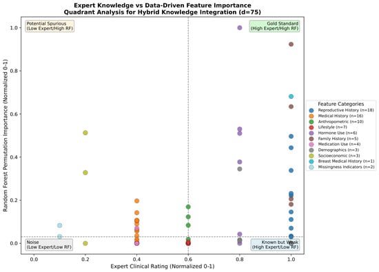
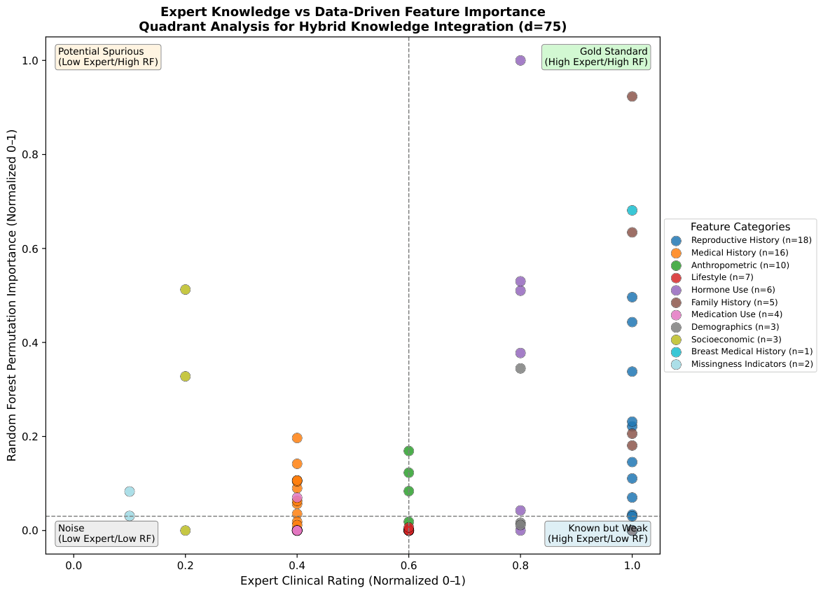
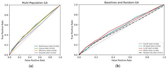
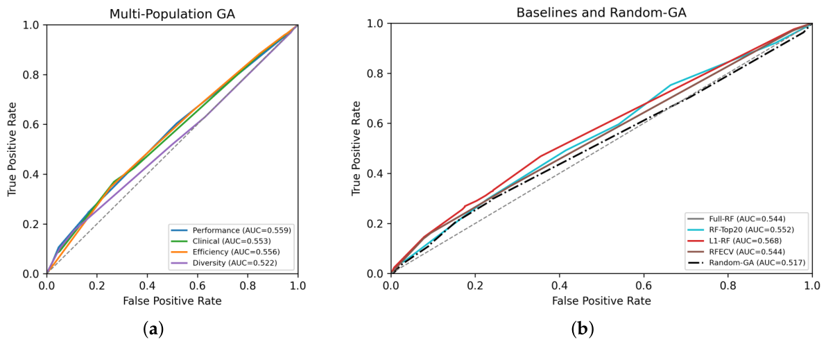
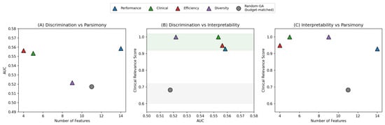
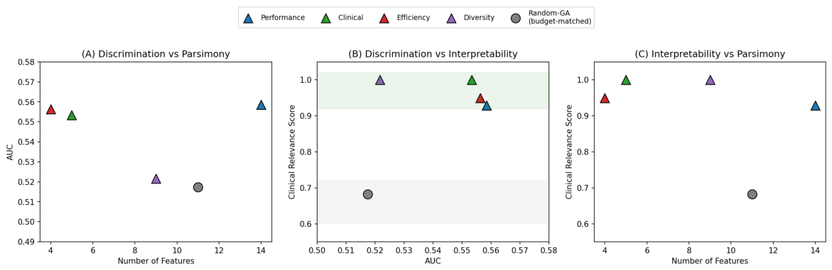

Disclaimer/Publisher’s Note: The statements, opinions and data contained in all publications are solely those of the individual author(s) and contributor(s) and not of MDPI and/or the editor(s). MDPI and/or the editor(s) disclaim responsibility for any injury to people or property resulting from any ideas, methods, instructions or products referred to in the content. |
© 2026 by the authors. Licensee MDPI, Basel, Switzerland. This article is an open access article distributed under the terms and conditions of the Creative Commons Attribution (CC BY) license.