Fuzzification of a Projectile Motion Equation

Abstract

Due to the extension of the concept of interval arithmetic, fuzzy numbers, which are a specific category of fuzzy sets, are often favored for representing real-world phenomena that involve uncertainty. This paper deals with the fuzzification of projectile motion, a classical physical phenomenon observed in the real world, which leads to the construction of a triangular parabolic fuzzy number, referred to as a projectile fuzzy number (PFN), whose properties are analyzed and discussed in detail. The discussion also covers the arithmetic operations involving two PFNs, not only with the established alpha-cut method but also with an approximation method, preserving the shape after operations. The fuzzification of projectile motion is utilized once more to construct a fuzzy equivalence relation, known as a projectile fuzzy equivalence relation. It has been shown that the dissimilarity of the projectile fuzzy equivalence relation constitutes a metric, the formula for which is presented explicitly. The application part of the study illustrates the qualitative fuzzy data clustering of the Iris dataset, the cancer dataset, and the crude oil dataset by employing the established projectile fuzzy equivalence relation as a similarity measure among the data points.

1. Introduction

Although mathematical models may appear to possess a certain degree of robustness, they ultimately fail to adequately encapsulate the phenomena observed in the empirical world. This limitation stems from the complexity of real-world systems, as mathematical models are simplified representations of reality that capture only crisp, deterministic and precise information, leading to a gap between theory and empirical reality [1,2,3,4,5,6,7]. As the magnitude of this gap increases, the accuracy of the information regarding reality that is captured, as well as processed and generated by the models, correspondingly diminishes, and vice versa. Therefore, it is imperative to acknowledge the existence of imperfect information which results from the gap between the abstraction and the empirical domain, and rather than dismissing this gap, mathematical models should also input imperfect information so that credible inferences can be drawn from these models. Since uncertainty arises from imperfect information, this can be managed by incorporating uncertainty into mathematical models. Various manifestations of uncertainty are present, and the categories most frequently encountered are ambiguity, vagueness, imprecision, variability, and ignorance [8,9,10]. One of the principal sources of imperfect information is the cognitive process inherent in human cognition [11], and it is evident that this prevalent manifestation of uncertainty can be effectively elucidated through linguistic analysis [12,13]. For example, consider the assertion, “The vehicle that I purchased is new.” In this case, ambiguity arises from the interpretation of the term ‘new’, given that the seller’s definition of the term ‘new’ may not coincide with that of the buyer. Likewise, vagueness can also arise from the term ‘new’, as the cutoff age for “new” is not clear, lacking a definitive boundary, making it a graded concept without a binary threshold. On the other hand, imprecision arises due to lack of exact numerical detail; variability is caused by inhomogeneity, and ignorance by lack of evidence. Besides these, uncertainty is prevalent in real-world phenomena due to measurement inaccuracies, ambiguous procedures, and unpredictable contexts. Many types of uncertainty are removable if sufficient knowledge and sophisticated devices are used in measurements [14]. However, uncertainty due to randomness is unremovable and is handled by probability theory. Probability theory deals with the likelihood of occurrence of events. As a result, this theory is a nongraded concept with a binary threshold, and therefore uses classical or crisp sets to model uncertain events. Fuzzy set theory, on the other hand, is a graded concept and an ingenious tool to incorporate uncertainty—uncertainty due to impreciseness and vagueness is handled by fuzzy sets, and uncertainty due to variability and ignorance is handled by fuzzy measures [15,16].

A classical (crisp) set theory constitutes a model of reality that inadequately represents imperfect information, as this theoretical framework is fundamentally based on bivalent logic and establishes a clear, unequivocal boundary between the elements that are members of the set and those that are not members of the set. It assigns a characteristic function that maps the membership status of an element to a binary set of values $\{0,1\}$, where 0 means non-membership and 1 denotes membership. Fuzzy set theory, initially introduced by L.A. Zadeh in 1965 [17], as a generalization of the crisp set theory, functions as a comprehensive mathematical tool for tackling imperfect information by integrating multivalued logic into its theoretical framework. In contrast to the crisp set, the fuzzy set assigns a specific degree of membership to each element within a closed unit interval $[0,1]$, extending from 0 to 1. This is accompanied by the formulation of the membership function, which serves as a generalization of the characteristic function. For example, if A is a set in a universe U, then for all x in U, we say $\tilde{A}$ is a fuzzy set if x belongs to A with a membership degree ranging from 0 to 1. In other words, an element x may belong to a fuzzy set $\tilde{A}$ with different grades of truth. Accordingly, concepts from crisp set theory are naturally generalized. For example, complement, intersection, and union are modeled in multiple ways to account for graded truth, and are therefore not unique in fuzzy set theory, but are defined through fuzzy operators. Since its inception, fuzzy set theory has undergone significant advancement in various scientific fields and has demonstrated effectiveness in addressing practical challenges within fuzzy environments [18]. The methods used to address these complexities usually consist of either combining two or more specified fuzzy sets into a single output fuzzy set or connecting two or more specified fuzzy sets to represent degrees of association between them [17,19]. The first method is typically achieved by extending traditional arithmetic operations to fuzzy sets through the application of the extension principle. For instance, if $\tilde{A}$ and $\tilde{B}$ denote two fuzzy sets associated with universes $U_1$ and $U_2$, respectively, then these fuzzy sets $\tilde{A}$ and $\tilde{B}$ can be combined to form a new fuzzy set $\tilde{C}$ related to the universe $U_1\ast U_2$ by applying Zadeh’s extension principle [17,20] as $\tilde{C}\left(z\right)=\underset{z=x_1\ast x_2}{sup}min[\tilde{A}\left(x_1\right),\tilde{B}\left(x_2\right)]$, where ∗ is an operation such as +, −, ×, and ÷. The second method involves extending classical relational concepts to fuzzy sets by linking the memberships of specified fuzzy sets from distinct universes [21]. For example, a binary fuzzy relation connecting two universes $U_1$ and $U_2$ is a fuzzy set defined on the Cartesian product $U_1\times U_2$ characterized by its membership functions ${\mu }_{\tilde{R}}(x_1,x_2)$ that describe the degree to which $x_1$ is in relation with $x_2$, where $x_1\in U_1$ and $x_2\in U_2$. Connecting two membership degrees through the assignment of a relation is useful in modeling fuzzy concepts. Various types of complement, intersection (t-norms), and union (t-conorms) operators are utilized to create different kinds of fuzzy relations in various contexts [22,23]. Situations that require computational analysis mainly depend on the former method [24], while rule-based control systems [25,26], decision-making tasks [27,28], similarity evaluations [29,30], and logic and inferential reasoning [31,32] primarily rely on the latter method.

Despite the significant role that fuzzy sets play in human abstraction, reasoning, and decision-making processes, the development of quantitative fuzzy variables and the associated arithmetic operations for modeling imperfect information presents considerable challenges. This difficulty arises primarily from the necessity of establishing a meaningful membership function, which often requires subjective evaluations or data-driven evaluations. In the preceding example, the allocation of membership grades to the term “new” poses a challenge, as it remains unclear which membership functions—triangular, Gaussian, or sigmoid [33,34]—most accurately encapsulate the concept of “new”. An inappropriate selection of the membership function could result in either an overestimation or an underestimation of the term “new”. Furthermore, even after careful identification of the membership function, there is no universally valid arithmetic rule in fuzzy arithmetic, unlike in crisp sets. This indicates that a variety of approaches exist for extending arithmetic principles within fuzzy arithmetic, and the selection of the appropriate rules demands domain-specific calibration, which is intrinsically challenging. For instance, the generalization of crisp mathematical concepts to fuzzy sets through the Zadeh extension principle [17,20] employing min and max operators may not yield satisfactory valuations of arithmetic operations, or the outcomes may be ambiguous owing to the inappropriateness of these operators. Moreover, the interpretation of outcomes or results derived from fuzzy arithmetic requires the process of defuzzification, which subsequently involves additional approximations. Even in a hypothetical situation where all tasks, including the identification of the appropriate membership function, the selection of pertinent arithmetic principles, and the determination of the appropriate defuzzification methodology, are executed proficiently, the computational process continues to be fundamentally iterative and considerably more complex than that associated with crisp sets.

This challenge led to the development of a specific type of fuzzy set called a fuzzy number, introduced by Zadeh [20], with major contributions from S. Nahmias [35], Dubois and Prade [36], and Kaufmann and Gupta [37]. The fuzzy number is a normalized (one element must have full membership) and convex (single peak) fuzzy set of the real line that has a continuous or upper semi-continuous membership function. The foremost advantage of a fuzzy number resides in its ability to be conceptualized with a specific shape (such as triangular, sigmoid, Gaussian, etc.), and it is this shape of a fuzzy number that determines its membership function. Furthermore, the practicality of fuzzy numbers is evident in their interpretation as subsets of real numbers, specifically, a closed interval within the set of real numbers, whereby arithmetic operations can be perceived as operations involving intervals. Among the diverse methodologies associated with fuzzy arithmetic, the alpha-cut method emerges as a conventional approach based on interval arithmetic [38], utilized to carry out a variety of arithmetic operations on fuzzy numbers. Consequently, interval arithmetic permits a more efficient execution of arithmetic operations, as it aligns with established arithmetic principles. Notably, Zadeh’s extension principle [17,20] aligns with the alpha-cut method, despite the fact that neither approach guarantees the preservation of the shape of a fuzzy number, particularly following multiplication [39]. The former method is comparatively slower, more complex to implement, and restricted to specific shapes when contrasted with the latter method. Moreover, the fuzzy number facilitates effective defuzzification through centroid or weighted average techniques [40,41], which are both quicker and more interpretable than the defuzzification of arbitrary fuzzy sets. However, the principal challenge lies in identifying the simplest and expressible shape that effectively encapsulates the desired fuzziness of the system to be modeled. Theoretically, a suitable fuzzy number that accurately represents the system under study can be determined by modeling vagueness through its shape or membership function, and imprecision through its interval.

Given the challenges of representing imperfect information, the need for computational efficiency, and the relevance to real-world applications, various shapes of fuzzy numbers are carefully chosen to model the system under study. Among the array of fuzzy number shapes, the triangular fuzzy number (TFN) and the Gaussian fuzzy number (GFN) emerge as two fundamentally distinct types [42,43]. The TFN is characterized by its simplicity, enhanced human interpretability, and computational convenience due to its closed-form arithmetic (exact for addition and approximate for multiplication). The GFN, on the other hand, is noted for its smoothness and mathematical elegance; however, it is marked by reduced human interpretability and heightened computational demands due to the absence of closed-form arithmetic (necessitating alpha-cut discretizations or approximations) and the involvement of exponential functions. Furthermore, the TFN works well for systems where imperfect information spreads linearly but struggles with smooth transitions. On the other hand, the GFN is better for modeling natural phenomena, which often change in nonlinear, smooth, and symmetrical ways rather than abruptly. The PFN is conceptualized based on the kinematics that a particle thrown vertically upward under gravity possesses crisp information, while increasing deviation from the vertical trajectory corresponds to a progressive loss of crisp information. The presence of resistance offered by the medium could further provide a useful basis for modeling external constraints imposed on the system, which can yield different parabolic shapes corresponding to different levels of fuzziness. However, to simplify the analysis, we have neglected such external constraints in the present study. This paper studies a PFN, which amalgamates the advantageous characteristics of both the TFN and the GFN, functioning as a singular shape fuzzy number that effectively addresses the deficiencies inherent in both the TFN and the GFN. Analogous to the GFN, the PFN is also suitable for representing nonlinear, smooth, and symmetrical transitions. At the same time, it can be easily transformed into its corresponding symmetric TFN for closed-form arithmetic. Therefore, the PFN can be a good choice to model the system where one has no prior information on how fuzziness propagates through it.

As previously stated, conducting arithmetic operations on PFNs offers numerous advantages in the computational analysis of systems. At times, it becomes more essential to find the relationships of different fuzzy sets from distinct universes rather than executing arithmetic operations. In the field of data analysis, finding a relation of a set onto itself has much significance, and one such area is data clustering, which involves assessing the similarity among different data points of a dataset. Fuzzy data clustering, particularly the hierarchical clustering method, often requires the construction of an appropriate fuzzy equivalence relation, and the desired clusters are formed by the suitable alpha-cut of this relational matrix [44,45]. An equivalence or similarity relation is a special type of a binary relation of a set with itself that is reflexive, symmetric and transitive, and constructing a similarity relational matrix in accordance with the transitive property is an important component in hierarchical clustering [21]. Moreover, transitivity defined under different t-norms yields different grades of similarity, making fuzzy equivalence relations useful for generalizing the concepts of similarity and equality. It is well known that similarity measures and distance measures are related concepts [46]. Every bounded distance measure $0\le d(x,y)\le 1$ can be regarded as a fuzzy dissimilarity relation, where a distance measure $d:X\times X\to {\mathbb{R}}^{+}$ satisfies $d(x,x)=0$, $d(x,y)=d(y,x)$ and $d(x,y)>0$ for $x\ne y$, for all $x,y\in X$. If $d(x,y)=0$ is allowed for some $x\ne y$, then d defines a pseudo-distance. When the triangle inequality is imposed, distance (pseudo-distance) measures form metrics (pseudo-metrics). In this paper, a fuzzy equivalence relation is developed by further fuzzifying projectile motion. An increasing generator is first derived from the projectile’s trajectory, and then, using the characterization theorem, the complement, union, and intersection operators are obtained from this generator. The concept of tautology is subsequently extended within the fuzzy framework, leading to the formulation of an equivalence relation. The relationship between this projectile-based fuzzy equivalence relation and generalized metrics is also examined. Finally, as a practical application, the constructed equivalence relation is tested in data clustering using the Iris [47], cancer [48], and crude oil [49] datasets.

This paper is systematically structured as follows. Section 2 outlines essential fuzzy mathematical concepts. Section 3 presents the formulation of a PFN along with important propositions that provide a comprehensive understanding of a PFN. Thereafter, a transformation of a PFN into an alternative representation is presented which is more intuitive and expressive within the domain of fuzzy arithmetic. Section 4 presents the development of a projectile fuzzy equivalence relation, explains its duality with generalized metrics, and reports the clustering results for the datasets.

2. Preliminaries

In this section, we introduce the basic terminology and notation required to understand the subsequent results. Definitions 1–13 are adopted from the sources [50,51], and Definitions 14–16 are adopted from sources [52,53].

Definition 1.

Let X be a universal set. A fuzzy set $\tilde{A}$ in X is a set of ordered pairs $\tilde{A}=\{(x,{\mu }_{\tilde{A}}\left(x\right)):x\in X\}$, where ${\mu }_{\tilde{A}}:X\to [0,1]$ is called a membership function.

A fuzzy set $\tilde{A}$ contains the elements of X with varying membership grades from 0 to 1. Certain elements may have a membership grade of 0, and it is often suitable to consider those elements of X that possess a non-zero degree of membership in $\tilde{A}$. This leads to numerous significant properties of a fuzzy set. Some of them are outlined in Definitions 2–6.

Definition 2.

An α-cut of a fuzzy set $\tilde{A}$ within a universal set X is the crisp set of all $x\in X$ such that ${\mu }_{\tilde{A}}\left(x\right)\ge \alpha$, where $\alpha \in [0,1]$.

Definition 3.

The support of a fuzzy set $\tilde{A}$ within a universal set X is the crisp set of all $x\in X$ such that ${\mu }_{\tilde{A}}\left(x\right)>0$.

Definition 4.

The core of a fuzzy set $\tilde{A}$ within a universal set X is the crisp set of all $x\in X$ such that ${\mu }_{\tilde{A}}\left(x\right)=1$.

Definition 5.

A fuzzy set $\tilde{A}$ within a universal set X is normal if there exists an $x\in X$ such that ${\mu }_{\tilde{A}}\left(x\right)=1$.

Definition 6.

A fuzzy set $\tilde{A}$ within a universal set X is convex if ${\mu }_{\tilde{A}}(\lambda x_1+(1-\lambda )x_2)\ge min\{{\mu }_{\tilde{A}}\left(x_1\right),{\mu }_{\tilde{A}}\left(x_2\right)\}$, $\forall x_1,x_2\in X$, $\lambda \in [0,1]$.

Among various fuzzy sets, those defined on the real line (i.e., with universal set $X=\mathbb{R}$) are commonly called fuzzy numbers and offer advantages in computational efficiency and simplicity for modeling uncertainty.

Definition 7.

A fuzzy number $\tilde{A}$ is a normal and convex fuzzy set $\tilde{A}$, characterized by an upper semi-continuous or continuous membership function with bounded support that is a subset of the real line $\mathbb{R}$.

A fuzzy number $\tilde{A}$ is called a positive if its membership function ${\mu }_{\tilde{A}}\left(x\right)=0$ $\forall x\le 0$. Otherwise, it is called a negative. As a fuzzy number extends the concept of an interval, arithmetic on fuzzy numbers follows the same rules as interval arithmetic. The membership function of the resulting fuzzy number is thus obtained via the inverse of the alpha-cut, which is the well-known alpha-cut method.

In the following Definitions 8–10, we present the terminology related to the complement operator, intersection operator or triangular norm (t-norm), and union operator or triangular conorm (t-conorm).

Definition 8.

A complement of a fuzzy set $\tilde{A}$ is a function $c:[0,1]\to [0,1]$ that satisfies the following conditions:

(i) 

$c\left(0\right)=1$ and $c\left(1\right)=0$.

(ii) 

$c\left(a\right)\ge c\left(b\right)$ whenever $a\le b$ $\forall a,b\in [0,1]$.

For practical significance, the two extra desirable conditions are usually listed in the notion of fuzzy complements. They are the following:

(iii)

c is a continuous function.

(iv)

c is involutive, i.e., $c\left(c\right(a\left)\right)=a$, $\forall a\in [0,1]$.

Definition 9.

A fuzzy intersection or t-norm is the binary operator $i:[0,1]\times [0,1]\to [0,1]$ that satisfies the following conditions:

(i) 

$i(a,1)=a$.

(ii) 

$i(a,b)=i(b,a)$.

(iii) 

$i(a,b)\le i(a,d)$ whenever $b\le d$.

(iv) 

$i(a,i(b,d\left)\right)=i\left(i\right(a,b),d)$.

Definition 10.

A fuzzy union or t-conorm is the binary operator $u:[0,1]\times [0,1]\to [0,1]$ that satisfies the following conditions:

(i) 

$u(a,0)=a$.

(ii) 

$u(a,b)=u(b,a)$.

(iii) 

$u(a,b)\le u(a,d)$ whenever $b\le d$.

(iv) 

$u(a,u(b,d\left)\right)=u\left(u\right(a,b),d)$.

Unlike crisp sets, fuzzy complement, intersection, and union operators are not unique; different classes of increasing generators can be used to construct various fuzzy complement, intersection, and union operators.

Definition 11.

An increasing generator is a strictly increasing continuous function $g:[0,1]\to \mathbb{R}$, with $g\left(0\right)=0$.

The notion of an increasing generator together with an involutive complement c is useful to generate a t-norm and a t-conorm that are dual with respect to c, that is, the triple $(i,u,c)$ satisfies the De Morgan laws for fuzzy sets. The next theorem, also known as the characterization theorem, explains this notion.

Theorem 1.

Given an involutive fuzzy complement c and an increasing generator g of c, the t-norm and t-conorm generated by g are dual with respect to c. Mathematically, for any $a,b\in [0,1]$, we have

• $c\left(a\right)=g^{-1}(g\left(1\right)-g\left(a\right))$,
• $i(a,b)=g^{(-1)}(g\left(a\right)+g\left(b\right)-g\left(1\right))$,
• $u(a,b)=g^{(-1)}(g\left(a\right)+g\left(b\right))$,
• where $g^{(-1)}$ is a pseudo-inverse, defined as

$$g^{(-1)}\left(a\right)=\left\{\begin{array}{cc}0\hfill & \mathit{for}a\in (-\infty ,0)\hfill \\ g^{-1}\left(a\right)\hfill & \mathit{for}a\in [0,g(1\left)\right]\hfill \\ 1\hfill & \mathit{for}a\in \left(g\right(1),\infty )\hfill \end{array}\right.$$

Moreover, $(i,u,c)$ is a dual triple.

The concepts of the complement operator, intersection operator, and union operator are instrumental in defining fuzzy implications by extending the notion of classical bivalent logic to fuzzy multivalued logic. Additionally, these operators play a significant role in linking fuzzy sets by establishing appropriate relationships. The next definition introduces a fuzzy binary relation, which can also be generalized to a fuzzy unary relation.

Definition 12.

Let X and Y be two non-empty sets. A fuzzy binary relation $\tilde{R}$ is a fuzzy set of the cartesian product $X\times Y$, and is defined as a set of ordered pairs $\tilde{R}=\{(x,y),{\mu }_{\tilde{R}}(x,y):(x,y)\in X\times Y\}$.

If $X=Y$, we define $\tilde{R}$ as a binary fuzzy relation on X. Among the various kinds of fuzzy binary relations, this paper focuses on fuzzy similarity or equivalence relations, which will be outlined in the next definitions.

Definition 13.

A fuzzy binary relation $\tilde{R}$ on X is a fuzzy equivalence relation if it fulfills the following conditions

(i) 

Reflexivity:${\mu }_{\tilde{R}}(x_1,x_1)=1$ $\forall x_1\in X$.

(ii) 

Symmetry: ${\mu }_{\tilde{R}}(x_1,x_2)={\mu }_R(x_2,x_1)$ $\forall x_1,x_2\in X$.

(iii) 

Transitivity: ${\mu }_{\tilde{R}}(x_1,x_3)\ge min({\mu }_R(x_1,x_2),{\mu }_{\tilde{R}}(x_2,x_3))$ $\forall x_1,x_2,x_3\in X$.

A fuzzy binary relation that is only reflexive and symmetric is known as a fuzzy compatibility or tolerance relation. As noted earlier, a bounded distance (pseudo-distance) measure can be interpreted as a fuzzy dissimilarity relation and is inversely related to a fuzzy compatibility relation. Transitivity can be modeled in multiple ways, not only with the standard fuzzy intersection (min-transitivity) but also using other t-norms. Thus, for an appropriate t-norm, every fuzzy compatibility relation is a fuzzy i-equivalence relation. With the inclusion of transitivity, this dual (two-sided inverse) relationship between a fuzzy i-equivalence relation ‘E’ and a u-metric (generalized metric) ‘d’ can be extended and expressed as $d(x_1,x_2)=f\left(E(x_1,x_2)\right)$, where f is a decreasing function with $f\left(0\right)=1$. Definitions 14 and 15 show the dual relationship between a fuzzy i-equivalence relation and a u-metric (or pseudo-u-metric).

Definition 14.

A fuzzy binary relation $\tilde{R}$ on X is a fuzzy i-equivalence relation if it fulfills the following conditions:

(i) 

Reflexivity: ${\mu }_{\tilde{R}}(x_1,x_1)=1$ $\forall x_1\in X$.

(ii) 

Symmetry: ${\mu }_{\tilde{R}}(x_1,x_2)={\mu }_{\tilde{R}}(x_2,x_1)$ $\forall x_1,x_2\in X$.

(iii) 

i-Transitivity: ${\mu }_{\tilde{R}}(x_1,x_3)\ge i({\mu }_{\tilde{R}}(x_1,x_2),{\mu }_{\tilde{R}}(x_2,x_3))$ $\forall x_1,x_2,x_3\in X$.

Definition 15.

A distance (or pseudo-distance) d on X is a u-metric (or pseudo-u-metric) if it fulfills the following conditions

(i) 

Reflexivity: $d(x_1,x_1)=0$ $\forall x_1\in X$.

(ii) 

Symmetry: $d(x_1,x_2)=d(x_2,x_1)$ $\forall x_1,x_2\in X$.

(iii) 

u-Triangular inequality: $d(x_1,x_3)\le u(d(x_1,x_2),d(x_2,x_3))$ $\forall x_1,x_2,x_3\in X$.

It should be noted that the type of t-conorm determines the form of the u-metric (generalized metric). For example, the bounded sum t-conorm yields the standard triangle inequality, producing a metric (or pseudo-metric) and the pair $(X,d)$ as a metric (or pseudo-metric) space. In contrast, using the standard union t-conorm leads to an ultrametric (or pseudo-ultrametric).

Among numerous applications, the usefulness of developing fuzzy equivalence relations in pattern recognition and cluster analysis is one of the acknowledged ones. Clustering is a technique of unsupervised data analysis where the dataset is partitioned into multiple subsets, guaranteeing that the data within the same subset exhibits similarity, while the data in different subsets shows dissimilarity based on some predefined similarity criteria. Such subsets are called clusters, and the fuzzy equivalence relation is used as a measure of similarity criteria, particularly in the hierarchically based fuzzy clustering algorithm. Definition 16 presents the notion of a cluster together with the clustering algorithm used in this paper.

Definition 16.

A subset $C(j;s)$ of $\{O_1,\dots ,O_N\}$ is called an $s_o$ neighborhood of $O_j$, iff $C(j;s)=\{O_k,k\in \{1,\dots ,N\}:{\mu }_{\tilde{R}}(j,k)\ge s_o\}$.

3. Projectile Fuzzy Number

3.1. Definitions

A PFN is constructed from the trajectory of a projectile motion, and hence the name. The equation for a projectile’s trajectory with initial velocity u and angle of projection $\theta$ is given by [54]

$$y=xtan\theta -{\displaystyle \frac{g{x}^2}{2u^{2}co{s}^2\theta }}$$

(1)

where g is the acceleration due to gravity. Likewise, the range and the maximum height attained by the projectile are, respectively,

$$\begin{array}{cc}\hfill R& ={\displaystyle \frac{u^{2}sin2\theta }{g}}\hfill \\ \hfill H& ={\displaystyle \frac{u^{2}si{n}^2\theta }{2g}}\hfill \end{array}$$

(2)

Using Equation (2) and replacing $tan\theta$ from Equation (1) by ${\displaystyle \frac{4H}{R}}$ results in

$$y={\displaystyle \frac{4xH}{R}}(1-{\displaystyle \frac{x}{R}})$$

(3)

For fuzzification, i.e., $y\in [0,1]$, H is taken as unity, which yields

$$y={\displaystyle \frac{4x}{R}}(1-{\displaystyle \frac{x}{R}})$$

(4)

Generalizing Equation (4), one can define the projectile fuzzy membership function as

$$\begin{array}{c}\hfill {\mu }_{P\tilde{F}N}\left(x\right)=\left\{\begin{array}{cc}{\displaystyle \frac{4(x-a)}{(b-a)}}\left(1-{\displaystyle \frac{(x-a)}{(b-a)}}\right),\hfill & a\le x\le b\hfill \\ 0,\hfill & \mathrm{otherwise}\hfill \end{array}\right.\end{array}$$

(5)

The following proposition is sufficient to show that the projectile fuzzy membership function is a fuzzy number.

Proposition 1.

Let $\tilde{A}$ be a fuzzy set defined in the real line $\mathbb{R}$ as a set of ordered pairs:

$$\tilde{A}=\left\{(x,{\mu }_{\tilde{A}}\left(x\right))\right|x\in \mathbb{R}\}$$

(6)

Then, $\tilde{A}$ is a projectile fuzzy number if ${\mu }_{\tilde{A}}\left(x\right):\mathbb{R}\to [0,1]$ is a projectile membership function.

Proof. 

In order to prove that $\tilde{A}$ is a fuzzy number, one needs to show that it is a convex normalized fuzzy set. Referring to Equation (5), let $x_o\in \mathbb{R}$ be defined as

$$x_o={\displaystyle \frac{(b+a)}{2}}$$

(7)

Then, one can easily see that ${\mu }_{\tilde{A}}\left(x_o\right)=1$, which shows that $\tilde{A}$ is a normal fuzzy set. Likewise, the $\alpha$- level set of $\tilde{A}$ is $A_{\alpha }=[A_L\left(\alpha \right),A_U\left(\alpha \right)]$ which is

$$A_{\alpha }=\left[{\displaystyle \frac{(b+a)-(b-a)\sqrt{(1-\alpha )}}{2}},{\displaystyle \frac{(b+a)+(b-a)\sqrt{(1-\alpha )}}{2}}\right]$$

(8)

It is easier to see that ∀$\alpha \in [0,1]$, the lower bound $A_L\left(\alpha \right)$ and the upper bound $A_U\left(\alpha \right)$ are finite and $A_L\left(\alpha \right)$ ≤ $A_U\left(\alpha \right)$, which shows that the alpha-level set is bounded and a single closed interval. Hence, $\tilde{A}$ is a convex fuzzy set.    □

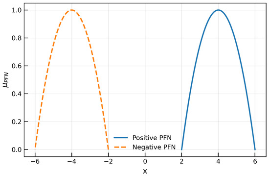
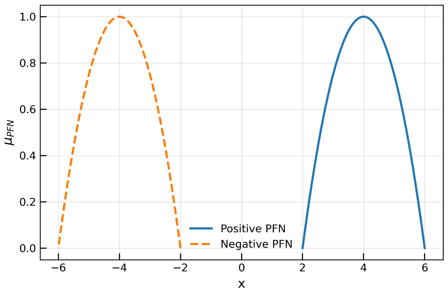
The positive and negative PFNs are shown in Figure 1. A negative PFN is simply the mathematical construction by choosing negative a and b. As the range of the projectile motion is positive, this paper deals with positive PFNs. The lower–upper representation $[A_L\left(\alpha \right),A_U\left(\alpha \right)]$ of a PFN, shown by Equation (8), is particularly useful for interval-based arithmetic. Based on the definition of the membership function, shown by Equation (5), it is also easier to represent PFN in duplet form as ${\tilde{A}}_{PFN}=(a,b)$.

Figure 1. Positive and negative PFNs.

Proposition 2.

Let $\tilde{A}=\left\{(x,{\mu }_{\tilde{A}}\left(x\right))\right|x\in \mathbb{R}\}$ be a triangular fuzzy number whose membership function is defined as

$$\begin{array}{c}\hfill {\mu }_{\tilde{A}}\left(x\right)=\left\{\begin{array}{cc}{\displaystyle \frac{(x-a)}{(x_o-a)}},\hfill & a\le x<x_o\hfill \\ 1,\hfill & x=x_o\hfill \\ {\displaystyle \frac{(b-x)}{(b-x_o)}},\hfill & x_o<x\le b\hfill \\ 0,\hfill & \mathit{otherwise}\hfill \end{array}\right.\end{array}$$

(9)

If $\tilde{A}$ is symmetric about $x=x_o$, then the projectile fuzzy number is defined by the following membership function:

$$\begin{array}{c}\hfill {\mu }_{P\tilde{F}N}\left(x\right)=\left\{\begin{array}{cc}{\displaystyle \frac{(x-a)}{(x_o-a)}}{\displaystyle \frac{(b-x)}{(b-x_o)}},\hfill & a\le x\le b\hfill \\ 0,\hfill & otherwise\hfill \end{array}\right.\end{array}$$

(10)

Proof. 

Symmetric $\tilde{A}$ results in $(x_o-a)=(b-x_o)$, and substituting $x_o={\displaystyle \frac{(b+a)}{2}}$ in ${\displaystyle \frac{(x-a)}{(x_o-a)}}{\displaystyle \frac{(b-x)}{(b-x_o)}}$, it is easy to reckon that ${\mu }_{P\tilde{F}N}$ is indeed a projectile membership function.    □

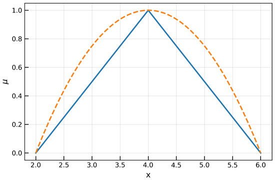
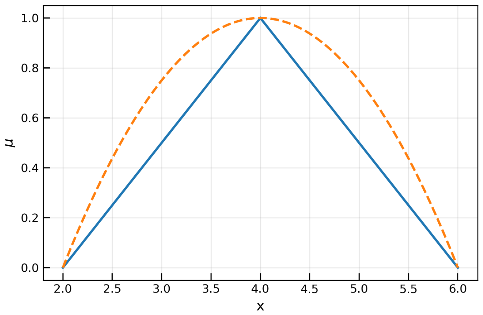
This proposition states that for every PFN, there exists a corresponding symmetric TFN inscribed, as illustrated in Figure 2. As previously mentioned, this attribute holds considerable importance, as the results derived from the modeling of a fuzzy system under linear approximation can be easily converted and compared to those from nonlinear approximation.

Figure 2. A PFN with an inscribed TFN.

A PFN can also be defined in terms of a parabolic fuzzy number [55,56]. The membership function of a parabolic fuzzy number $\tilde{A}$ is defined as

$$\begin{array}{c}\hfill {\mu }_{\tilde{A}}\left(x\right)=\left\{\begin{array}{cc}1-{\left({\displaystyle \frac{x_o-x}{x_o-a}}\right)}^2,\hfill & a\le x<x_o\hfill \\ 1,\hfill & x=x_o\hfill \\ 1-{\left({\displaystyle \frac{x-x_o}{b-x_o}}\right)}^2,\hfill & x_o<x\le b\hfill \\ 0,\hfill & \mathrm{otherwise}\hfill \end{array}\right.\end{array}$$

(11)

The following proposition tells us about that.

Proposition 3.

A symmetric or triangular parabolic fuzzy number is a PFN.

Proof. 

It is straightforward to see that by substituting $x_o={\displaystyle \frac{(b+a)}{2}}$ in Equation (11), the left- and right-shaped functions are the same and equal the projectile membership function.    □

3.2. Transformation of a PFN

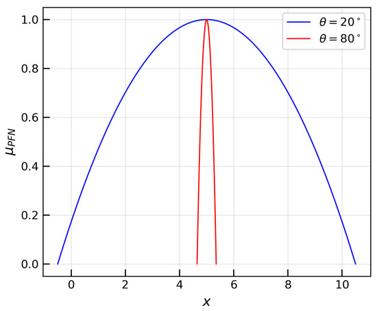
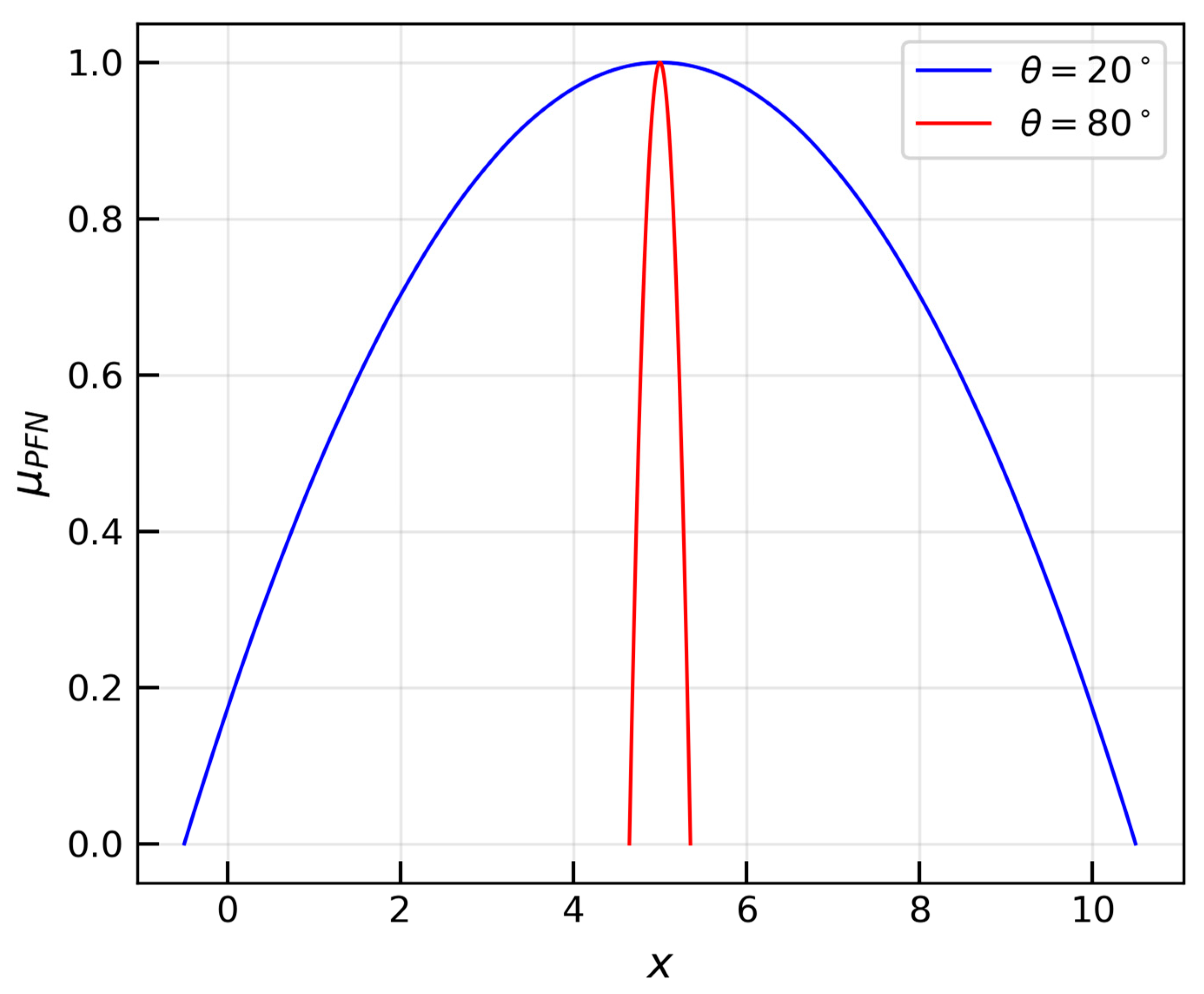
One may ask why the projectile motion trajectory is used instead of a simple parabolic function. The reason lies in the transformation of a PFN. A PFN $\tilde{A}=(a,b)$ can be represented as $\tilde{A}=(m,tan\theta )$, where m is the center (core) of $(a,b)$ and $tan\theta ={\displaystyle \frac{4}{b-a}}$, $0^{\circ }<\theta <{90}^{\circ }$ being the projection angle. This representation offers two advantages: first, the level of imprecision is captured by a single parameter, the projection angle. That is, a larger projection angle corresponds to a lower level of imprecision as shown in Figure 3; when $\theta \to {90}^{\circ }$, the PFN reduces to a crisp number. Second, it simplifies arithmetic operations between PFNs, as discussed in the next subsection.

Figure 3. Two PFNs with the same core but different projection angles exhibit different levels of imprecision.

Proposition 4.

A PFN $\tilde{A}$ = $(a,b)$ is equivalent to $\tilde{A}$ = $(m,tan\theta )$.

Proof. 

By substituting $tan\theta ={\displaystyle \frac{4}{b-a}}$, it can be shown that the projectile fuzzy membership function described by Equation (5) can be transformed as

$$\begin{array}{c}\hfill {\mu }_{\tilde{A}}\left(x\right)=\left\{\begin{array}{cc}1-{\displaystyle \frac{ta{n}^2\theta }{4}}{(x-m)}^2,\hfill & m-{\displaystyle \frac{2}{tan\theta }}\le x\le m+{\displaystyle \frac{2}{tan\theta }}\hfill \\ 0,\hfill & \mathrm{otherwise}\hfill \end{array}\right.\end{array}$$

(12)

The $\alpha$-level set as described by Equation (8) can also be transformed as,

$$\tilde{A}=[m_1-{\displaystyle \frac{2}{tan\theta }}\sqrt{1-\alpha },m_1+{\displaystyle \frac{2}{tan\theta }}\sqrt{1-\alpha }]$$

   □

Similarly, an inscribed symmetric triangular fuzzy number $\tilde{A}$ can be defined in this notation as

$$\begin{array}{c}\hfill {\mu }_{\tilde{A}}\left(x\right)=\left\{\begin{array}{cc}1+{\displaystyle \frac{tan\theta (x-m)}{2}},\hfill & m-{\displaystyle \frac{2}{tan\theta }}\le x<m\hfill \\ 1,\hfill & x=m\hfill \\ 1-{\displaystyle \frac{tan\theta (x-m)}{2}},\hfill & m<x\le m+{\displaystyle \frac{2}{tan\theta }}\hfill \\ 0,\hfill & \mathrm{otherwise}\hfill \end{array}\right.\end{array}$$

(13)

3.3. Arithmetic Operations

Arithmetic operations on fuzzy numbers using the alpha-cut method or the extension principle are exact. The motivation of this paper is to develop alternative closed-form approaches for such computations. There are two such approaches for arithmetic operations on two PFNs. The first approach converts each PFN into its corresponding inscribed TFN (Proposition 2), performs arithmetic on the TFNs—exact for addition and subtraction, and approximately exact for multiplication and division—and then converts the result back to a PFN. Although this approach is straightforward and computationally efficient, this paper focuses on the second approach, where representing PFNs as $(m,tan\theta )$ significantly simplifies the arithmetic operations. Let two PFNs be given as $\tilde{A}$ = $(a_1,a_2)$ = $(m_1,tan{\theta }_1)$ and $\tilde{B}$ = $(b_1,b_2)$ = $(m_2,tan{\theta }_2)$. Their arithmetic operation yields $\tilde{C}$ = $(c_1,c_2)$ = $(m,tan\theta )$ where $\tilde{C}=\tilde{A}\ast \tilde{B}$ is a fuzzy number. Then, it is useful to note the following points:

(i)

Arithmetic operations on the cores follow the standard real number operations; thus, $m=m_1\ast m_2$.

(ii)

Since the core operation is exact, the resulting left and right spreads calculated from the core equation match those obtained via the alpha-cut method. If these spreads are equal, then $\tilde{C}$ is a PFN.

(iii)

If $\tilde{C}$ is a PFN, then $tan\theta$ depends only on $tan{\theta }_1$ and $tan{\theta }_2$. If $\tilde{C}$ is not a PFN, then $tan\theta$ also depends on $m_1$ and $m_2$. In such cases, $\tilde{C}$ can be approximated as a PFN by suitably defining m in terms of $m_1$, $m_2$, $tan{\theta }_1$ and $tan{\theta }_2$, that is, violating the core equation, $m\ne m1\ast m2$.

(iv)

In the approximation method, $\tilde{C}$ is assumed to be a PFN with $m={\displaystyle \frac{c_1+c_2}{2}}$ and $tan\theta ={\displaystyle \frac{4}{c_2-c_1}}$. From these, m is expressed in terms of $m_1$ and $m_2$, and $tan\theta$ in terms of $tan{\theta }_1$ and $tan{\theta }_2$. If m satisfies the core equation and $tan\theta$ depends only on $tan{\theta }_1$ and $tan{\theta }_2$, then $\tilde{C}$ is a PFN; otherwise, it is not.

(v)

In the converse method, we start from the core equation and determine the left and right spreads. If the spreads are equal, then $\tilde{C}$ is a PFN; otherwise, it is not.

The following propositions justify these points.

Proposition 5 (Alpha-cut Method).

The addition of two PFNs results in the generation of another PFN.

Proof. 

Let $\tilde{A}=(a_1,a_2)$, which is transformed to $(m_1,tan{\theta }_1)$, and $\tilde{B}=(b_1,b_2)$, which is transformed to $(m_2,tan{\theta }_2)$, be two PFNs. Then, the lower–upper representations of these PFNs are $A_{\alpha }=[m_1-{\displaystyle \frac{2}{tan{\theta }_1}}\sqrt{1-\alpha },m_1+{\displaystyle \frac{2}{tan{\theta }_1}}\sqrt{1-\alpha }]$ and $B_{\alpha }=[m_2-{\displaystyle \frac{2}{tan{\theta }_2}}\sqrt{1-\alpha },m_2+{\displaystyle \frac{2}{tan{\theta }_2}}\sqrt{1-\alpha }]$.

Now, $C_{\alpha }=A_{\alpha }+B_{\alpha }=[m_1+m_2-2\sqrt{1-\alpha }({\displaystyle \frac{1}{tan{\theta }_1}}+{\displaystyle \frac{1}{tan{\theta }_2}}),m_1+m_2+2\sqrt{1-\alpha }({\displaystyle \frac{1}{tan{\theta }_1}}+{\displaystyle \frac{1}{tan{\theta }_2}})]$.

The membership function of $\tilde{C}$ can be found by taking the inverse of $C_{\alpha }$:

$$\begin{array}{c}\hfill {\mu }_{\tilde{C}}\left(x\right)=\left\{\begin{array}{cc}1-{\displaystyle \frac{{(m_1+m_2-x)}^2}{4{(\frac{1}{tan{\theta }_1}+\frac{1}{tan{\theta }_2})}^2}},\hfill & c_1\le x\le c_2\hfill \\ 0,\hfill & \mathrm{otherwise}\hfill \end{array}\right.\end{array}$$

(14)

where $c_1=a_1+b_1$ and $c_2=a_2+b_2$. It is evident from the membership function that $\tilde{C}$ is a PFN. Thus, $\tilde{C}=(m,tan\theta )$ is a PFN, and it is easy to see that $m=m_1+m_2$ and $tan\theta ={\displaystyle \frac{tan{\theta }_{1}tan{\theta }_2}{(tan{\theta }_1+tan{\theta }_2)}}$.    □

Proposition 6.

The subtraction of two PFNs results in the generation of another PFN.

Proof. 

It is straightforward to see that $C_{\alpha }=A_{\alpha }-B_{\alpha }=A_{\alpha }+B_{\alpha }^{-}$, which results in

$$\begin{array}{c}\hfill {\mu }_{\tilde{C}}\left(x\right)=\left\{\begin{array}{cc}1-{\displaystyle \frac{{(m_1-m_2-x)}^2}{4{(\frac{1}{tan{\theta }_1}+\frac{1}{tan{\theta }_2})}^2}},\hfill & c_1\le x\le c_2\hfill \\ 0,\hfill & \mathrm{otherwise}\hfill \end{array}\right.\end{array}$$

(15)

Thus, $\tilde{C}=(m,tan\theta )$ is a PFN, where $m=m_1-m_2$ and $tan\theta ={\displaystyle \frac{tan{\theta }_{1}tan{\theta }_2}{(tan{\theta }_1+tan{\theta }_2)}}$.    □

Proposition 7 (Approximation Method).

Let $\tilde{A}=(m_1,tan{\theta }_1)$ and $\tilde{B}=(m_2,tan{\theta }_2)$ be two PFNs. If the addition of $\tilde{A}$ and $\tilde{B}$ yields another PFN, say, $\tilde{C}=(m,tan\theta )$, then $m=m_1+m_2$ and $tan\theta$ depends only on $tan{\theta }_1$ and $tan{\theta }_2$.

Proof. 

Assuming $\tilde{C}$ is a PFN, one can transform $(m,tan\theta )$ to $(c_1,c_2)$ such that $m={\displaystyle \frac{c_1+c_2}{2}}$ and $tan\theta ={\displaystyle \frac{4}{c_2-c_1}}$. Using interval arithmetic, one can rewrite $m={\displaystyle \frac{(a_1+b_1)+(a_2+b_2)}{2}}$ and $tan\theta ={\displaystyle \frac{4}{(a_2+b_2)-(a_1+b_1)}}$, where $(a_1,a_2)$ and $(b_1,b_2)$ are transformed from $(m_1,tan{\theta }_1)$ and $(m_2,tan{\theta }_2)$, respectively. As $\tilde{A}$ and $\tilde{B}$ are PFNs, substituting $a_1=m_1-{\displaystyle \frac{2}{tan{\theta }_1}}$, $a_2=m_1+{\displaystyle \frac{2}{tan{\theta }_1}}$, $b_1=m_2-{\displaystyle \frac{2}{tan{\theta }_2}}$ and $b_2=m_2+{\displaystyle \frac{2}{tan{\theta }_2}}$ yields $m=m_1+m_2$ and $tan\theta ={\displaystyle \frac{tan{\theta }_{1}tan{\theta }_2}{(tan{\theta }_1+tan{\theta }_2)}}$, which is dependent only on $tan{\theta }_1$ and $tan{\theta }_2$. Since the assumption that $\tilde{C}$ is a PFN leads to no contradiction, it follows that $\tilde{C}$ is indeed a PFN.    □

It is interesting to note that m and $tan\theta$ calculated from the approximation method match those from the alpha-cut method. The next proposition shows that the core equation of addition for two PFNs $\tilde{A}$ and $\tilde{B}$ is sufficient to calculate the left and right spreads of a fuzzy number $\tilde{C}$ such that $\tilde{C}=\tilde{A}+\tilde{B}$.

Proposition 8 (Converse Method).

Let $\tilde{A}$ and $\tilde{B}$ be two PFNs, and let $\tilde{C}=\tilde{A}+\tilde{B}$. If the core equation of addition yields uniform left and right spreads for $\tilde{C}$, then $\tilde{C}$ is also a PFN.

Proof. 

Starting from the core equation of addition, $m=m_1+m_2$. Now, for the left spread, we substitute $m_1=a_1+{\displaystyle \frac{2}{tan{\theta }_1}}$ and $m_2=b_1+{\displaystyle \frac{2}{tan{\theta }_2}}$ and for the right spread, $m_1=a_2-{\displaystyle \frac{2}{tan{\theta }_1}}$ and $m_2=b_2-{\displaystyle \frac{2}{tan{\theta }_2}}$. After substituting these values, it is easy to see that the spread on the left and the spread on the right of $\tilde{C}$ match with width 2(${\displaystyle \frac{1}{tan{\theta }_1}}$ + ${\displaystyle \frac{1}{tan{\theta }_2}})$, which in turn equals the spread calculated from the alpha-cut method. Therefore, $\tilde{C}$ is a PFN.    □

The converse method is the reverse of the approximation method: if one yields a PFN, so does the other, and vice versa.

Example 1.

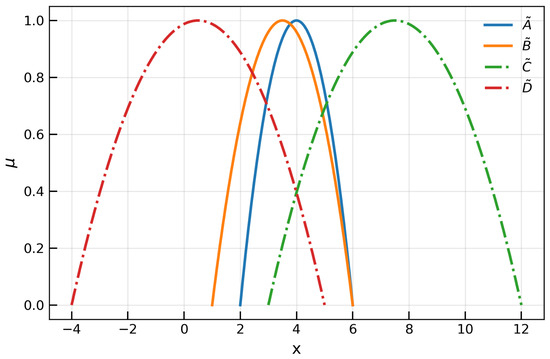
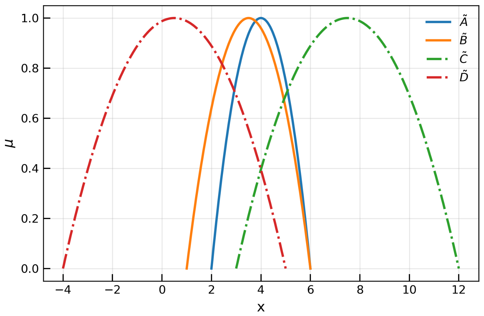
Consider $\tilde{A}=(a_1,a_2)=(2,6)$ and $\tilde{B}=(b_1,b_2)=(1,6)$ as two PFNs. Now, we add and subtract $\tilde{A}$ and $\tilde{B}$ using both methods—the alpha-cut method and the approximation method. At first, $\tilde{A}$ and $\tilde{B}$ are transformed in the form $(m_1,tan{\theta }_1)=(4,1)$ and $(m_2,tan{\theta }_2)=(7/2,4/5)$, respectively. It is easy to see that both methods, as illustrated in Propositions 5–7, yield the same PFN, say $\tilde{C}=(m,tan\theta )=(15/2,4/9)$ as the sum of $\tilde{A}$ and $\tilde{B}$, and $\tilde{D}=(m,tan\theta )=(1/2,4/9)$ as the difference of $\tilde{A}$ and $\tilde{B}$, as shown in Figure 4.

Figure 4. The sum of two PFNs, $\tilde{A}$ and $\tilde{B}$, yields a new PFN $\tilde{C}$, identical to that obtained using the alpha-cut and approximation methods.

It is well known that the multiplication of two fuzzy numbers results in the generation of another fuzzy number; however, due to the nonlinear nature of this operation, the shape of the resultant fuzzy number is not preserved, leading to a distortion that diminishes both the simplicity and the interpretability of the results. Furthermore, the first approach proves to be advantageous, as the multiplication operations between two triangular fuzzy numbers can be readily approximated to a linear form. Given that this approximation is well established, we now focus on the second approach, following the same procedure as in the case of addition.

Proposition 9 (Alpha-cut Method).

The multiplication of two PFNs does not result in the generation of another PFN.

Proof. 

In this case, $C_{\alpha }=A_{\alpha }\times B_{\alpha }=[m_1{m}_2+{\displaystyle \frac{4(1-\alpha )}{tan{\theta }_{1}tan{\theta }_2}}-2\sqrt{1-\alpha }({\displaystyle \frac{m_1}{tan{\theta }_2}}+{\displaystyle \frac{m_2}{tan{\theta }_1}}),m_1{m}_2+{\displaystyle \frac{4(1-\alpha )}{tan{\theta }_{1}tan{\theta }_2}}+2\sqrt{1-\alpha }({\displaystyle \frac{m_1}{tan{\theta }_2}}+{\displaystyle \frac{m_2}{tan{\theta }_1}})]$.

The membership function of $\tilde{C}$ can be found by taking the inverse of $C_{\alpha }$:

$$\begin{array}{c}\hfill {\mu }_{\tilde{C}}\left(x\right)=\left\{\begin{array}{cc}1-{\left({\displaystyle \frac{(m_{1}tan{\theta }_1+m_{2}tan{\theta }_2)-\sqrt{{(m_{1}tan{\theta }_1+m_{2}tan{\theta }_2)}^2-4(m_1{m}_2-x)tan{\theta }_{1}tan{\theta }_2}}{4}}\right)}^2,\hfill & c_1\le x\le c_2\hfill \\ 0,\hfill & \mathrm{otherwise}\hfill \end{array}\right.\end{array}$$

(16)

where $c_1=a_1{b}_1$ and $c_2=a_2{b}_2$. It is evident from the membership function that $\tilde{C}$ is not a PFN. Thus, for $\tilde{A}=(m_1,tan{\theta }_1)$ and $\tilde{B}=(m_2,tan{\theta }_2)$, their product $\tilde{C}$ is not a PFN. It is easy to notice that $c_1$ is $m_1{m}_2+{\displaystyle \frac{4}{tan{\theta }_{1}tan{\theta }_2}}-2({\displaystyle \frac{m_1}{tan{\theta }_2}}+{\displaystyle \frac{m_2}{tan{\theta }_1}})$ and $c_2$ is $m_1{m}_2+{\displaystyle \frac{4}{tan{\theta }_{1}tan{\theta }_2}}+2({\displaystyle \frac{m_1}{tan{\theta }_2}}+{\displaystyle \frac{m_2}{tan{\theta }_1}})$.    □

Proposition 10.

The division of two PFNs does not result in the generation of another PFN.

Proof. 

In this case, $C_{\alpha }=A_{\alpha }/B_{\alpha }=[{\displaystyle \frac{m_1-\frac{2}{tan{\theta }_1}\sqrt{1-\alpha }}{m_2+\frac{2}{tan{\theta }_2}\sqrt{1-\alpha }}},{\displaystyle \frac{m_1+\frac{2}{tan{\theta }_1}\sqrt{1-\alpha }}{m_2-\frac{2}{tan{\theta }_2}\sqrt{1-\alpha }}}]$. The membership function of $\tilde{C}$ can be found by taking the inverse of $C_{\alpha }$:

$$\begin{array}{c}\hfill {\mu }_{\tilde{C}}\left(x\right)=\left\{\begin{array}{cc}1-{\displaystyle \frac{{(m_1-x{m}_2)}^2}{4{(\frac{1}{tan{\theta }_1}+\frac{x}{tan{\theta }_2})}^2}},\hfill & c_1\le x\le c_2\hfill \\ 0,\hfill & \mathrm{otherwise}\hfill \end{array}\right.\end{array}$$

(17)

where $c_1={\displaystyle \frac{a_1}{b_2}}$ and $c_2={\displaystyle \frac{a_2}{b_1}}$. Clearly, $\tilde{C}$ is not a PFN.    □

Proposition 11 (Approximation Method).

Let $\tilde{A}=(m_1,tan{\theta }_1)$ and $\tilde{B}=(m_2,tan{\theta }_2)$ be two PFNs. If the multiplication of $\tilde{A}$ and $\tilde{B}$ yields another PFN, say, $\tilde{C}=(m,tan\theta )$, then $m=m_1{m}_2$ and $tan\theta$ depends only on $tan{\theta }_1$ and $tan{\theta }_2$.

Proof. 

Assuming $\tilde{C}$ is a PFN, one can transform $(m,tan\theta )$ to $(c_1,c_2)$ such that $m={\displaystyle \frac{c_1+c_2}{2}}$ and $tan\theta ={\displaystyle \frac{4}{c_2-c_1}}$. Using interval arithmetic, one can rewrite $m={\displaystyle \frac{\left(a_1{b}_1\right)+\left(a_2{b}_2\right)}{2}}$ and $tan\theta ={\displaystyle \frac{4}{\left(a_2{b}_2\right)-\left(a_1{b}_1\right)}}$, where $(a_1,a_2)$ and $(b_1,b_2)$ are transformed $(m_1,tan{\theta }_1)$ and $(m_2,tan{\theta }_2)$, respectively. As $\tilde{A}$ and $\tilde{B}$ are PFNs, substituting $a_1=m_1-{\displaystyle \frac{2}{tan{\theta }_1}}$, $a_2=m_1+{\displaystyle \frac{2}{tan{\theta }_1}}$, $b_1=m_2-{\displaystyle \frac{2}{tan{\theta }_2}}$ and $b_2=m_2+{\displaystyle \frac{2}{tan{\theta }_2}}$ yields $m=m_1{m}_2+{\displaystyle \frac{4}{tan{\theta }_{1}tan{\theta }_2}}$, which violates the core equation, and $tan\theta ={\displaystyle \frac{tan{\theta }_{1}tan{\theta }_2}{(m_{1}tan{\theta }_1+m_{2}tan{\theta }_2)}}$, which is also dependent on $m_1$ and $m_2$. Since the assumption that $\tilde{C}$ is a PFN leads to contradiction, it follows that $\tilde{C}$ is not a PFN.

However, approximating $m=m_1{m}_2+{\displaystyle \frac{4}{tan{\theta }_{1}tan{\theta }_2}}$ and taking the same $tan\theta ={\displaystyle \frac{tan{\theta }_{1}tan{\theta }_2}{(m_{1}tan{\theta }_1+m_{2}tan{\theta }_2)}}$ results in the formation of a PFN of the same interval width. Similarly, approximating an exact quotient by a PFN is not particularly difficult. Once the approximation of an exact product by a PFN is established, the division case follows straightforwardly. The following proposition illustrates this.    □

Proposition 12.

Let $\tilde{A}$ and $\tilde{B}$ be two PFNs. If $\tilde{C}=\tilde{A}\times \tilde{B}$ and $\tilde{D}=\tilde{A}/\tilde{B}$ are PFNs, constructed using the approximation method, then their products of the core and the tangent angle are the same.

Proof. 

Let $\tilde{C}=(m,tan\theta )$ and $\tilde{D}=(m^{\ast },tan{\theta }^{\ast })$ be PFNs. Then, it is easy to see that $tan\theta ={\displaystyle \frac{4}{(a_2{b}_2-a_1{b}_1)}}$ and $tan{\theta }^{\ast }={\displaystyle \frac{4b_1{b}_2}{(a_2{b}_2-a_1{b}_1)}}$, where $\tilde{A}=(a_1,a_2)$ and $\tilde{B}=(b_1,b_2)$. This results in $tan{\theta }^{\ast }=tan\theta b_1{b}_2$. Similarly, $m={\displaystyle \frac{(a_2{b}_2+a_1{b}_1)}{2}}$ and $m^{\ast }={\displaystyle \frac{(a_2{b}_2+a_1{b}_1)}{2b_1{b}_2}}$. This results, $m=m^{\ast }{b}_1{b}_2$. Eliminating $b_1{b}_2$, one can reckon that $mtan\theta =m^{\ast }tan{\theta }^{\ast }$.    □

It is also interesting to note that the divisor factor (product of the divisor base points), “$b_1{b}_2$”, naturally comes into play whenever there is a correlation between $\tilde{C}$ and $\tilde{D}$. The following proposition illustrates the meaning of “$b_1{b}_2$”.

Proposition 13.

Let $\tilde{A}$ and $\tilde{B}$ be two PFNs. If $\tilde{C}=\tilde{A}\times \tilde{B}$ and $\tilde{D}=\tilde{A}/\tilde{B}$ are PFNs, constructed using the approximation method, then the divisor factor $b_1{b}_2$ is simply the ratio of the support width of $\tilde{C}$ to that of $\tilde{D}$.

Proof. 

Following Proposition 12, $b_1{b}_2={\displaystyle \frac{tan{\theta }^{\ast }}{tan\theta }}$. Using $c_2-c_1={\displaystyle \frac{4}{tan\theta }}$ and $d_2-d_1={\displaystyle \frac{4}{tan{\theta }^{\ast }}}$, it is easy to notice that $b_1{b}_2={\displaystyle \frac{c_2-c_1}{d_2-d_1}}$.    □

Furthermore, to quantify the precision loss in the shape-preserving approximation, we use the Hausdorff distance as an error metric. Since the support widths coincide and only the cores differ, the entire error is determined by the core difference. Thus, in this case, the Hausdorff distance is simply $({\delta }_H=|m_{exact}-m_{approx.}\left|\right)$. In the case of the multiplication operation, ${\delta }_H={\displaystyle \frac{4}{tan{\theta }_{1}tan{\theta }_2}}$, and the relative Hausdorff distance (normalizing with the support width) is ${\delta }_H^R={\displaystyle \frac{1}{m_{1}tan{\theta }_1+m_{2}tan{\theta }_2}}$. Similarly, in the case of the division operation, ${\delta }_H^{\ast }={\displaystyle \frac{\frac{4}{tan{\theta }_2}(\frac{m_1}{tan{\theta }_2}+\frac{m_2}{tan{\theta }_1})}{m_2(m_2^2-{\left(\frac{2}{tan{\theta }_2}\right)}^2)}}$, and ${\delta }_H^{\ast R}={\displaystyle \frac{1}{m_{2}tan{\theta }_2}}$. As we have seen that the divisor factor correlates between the approximated product and quotient PFNs, one can also express the divisor factor in terms of their respective Hausdorff distances, as illustrated by the next proposition.

Proposition 14.

Let ${\delta }_H$ or ${\delta }_H^R$ be the Hausdorff distance between the exact and approximate product and ${\delta }_H^{\ast }$ or ${\delta }_H^{\ast R}$ between the exact quotient and approximate quotient. The divisor factor satisfies $b_1{b}_2={\displaystyle \frac{{\delta }_H{\delta }_H^{\ast R}}{{\delta }_H^{\ast }{\delta }_H^R}}$.

Proof. 

It is straightforward to calculate ${\delta }_H^{\ast }={\displaystyle \frac{{\delta }_H}{b_1{b}_2}}(1+{\displaystyle \frac{m_{1}tan{\theta }_1}{m_{2}tan{\theta }_2}})$ or ${\delta }_H^{\ast R}={\delta }_H^R(1+{\displaystyle \frac{m_{1}tan{\theta }_1}{m_{2}tan{\theta }_2}})$. This yields $b_1{b}_2={\displaystyle \frac{{\delta }_H{\delta }_H^{\ast R}}{{\delta }_H^{\ast }{\delta }_H^R}}$.    □

Proposition 15 (Converse Method).

Let $\tilde{A}$ and $\tilde{B}$ be two PFNs, and let $\tilde{C}=\tilde{A}\times \tilde{B}$. If the core equation of multiplication yields uniform spreads on the left and right for $\tilde{C}$, then $\tilde{C}$ is also a PFN.

Proof. 

Starting from the core equation of multiplication, $m=m_1{m}_2$. Now, for the left spread, we substitute $m_1=a_1+{\displaystyle \frac{2}{tan{\theta }_1}}$ and $m_2=b_1+{\displaystyle \frac{2}{tan{\theta }_2}}$ and for the right spread, $m_1=a_2-{\displaystyle \frac{2}{tan{\theta }_1}}$ and $m_2=b_2-{\displaystyle \frac{2}{tan{\theta }_2}}$. After substituting these values, it is easy to see that the spread on the left is ${\displaystyle \frac{2(m_{1}tan{\theta }_1+m_{2}tan{\theta }_2-2)}{tan{\theta }_{1}tan{\theta }_2}}$ and the spread on the right is ${\displaystyle \frac{2(m_{1}tan{\theta }_1+m_{2}tan{\theta }_2+2)}{tan{\theta }_{1}tan{\theta }_2}}$, which do not match with each other. Hence, $\tilde{C}$ is not a PFN.    □

Since the core equation is exact, the left and right spreads match with the spread calculated from the alpha-cut method.

Example 2.

Consider $\tilde{A}=(a_1,a_2)=(2,6)$ and $\tilde{B}=(b_1,b_2)=(1,6)$ to be two PFNs. $\tilde{C}$ is the product of $\tilde{A}$ and $\tilde{B}$ using the alpha-cut method, and $\tilde{D}$ is a PFN using the approximation method. $\tilde{E}$ is the quotient of $\tilde{A}$ divided by $\tilde{B}$ using the alpha-cut method, and $\tilde{F}$ is a PFN using the approximation method as shown in Figure 5. Furthermore, in this example, ${\delta }_H^R=0.147$ or (${\delta }_H=5$), and ${\delta }_H^{\ast R}=0.357$ or (${\delta }_H^{\ast }=2.026$).

Figure 5. The product and quotient of two PFNs, $\tilde{A}$ and $\tilde{B}$, using the alpha-cut method result in new fuzzy numbers $\tilde{C}$ and $\tilde{E}$, respectively, which are not PFNs. The approximation method, on the other hand, yields corresponding PFNs $\tilde{D}$ and $\tilde{F}$, respectively.

4. Projectile-Increasing Generator

The aim of this section is to show that the physical trajectory acts as a kinematic generation mechanism for the well-established fuzzy connectives.

4.1. Definitions

Starting from Equation (3), it is straightforward to see that

$$y=xtan\theta -{\displaystyle \frac{x^2}{R}}tan\theta$$

(18)

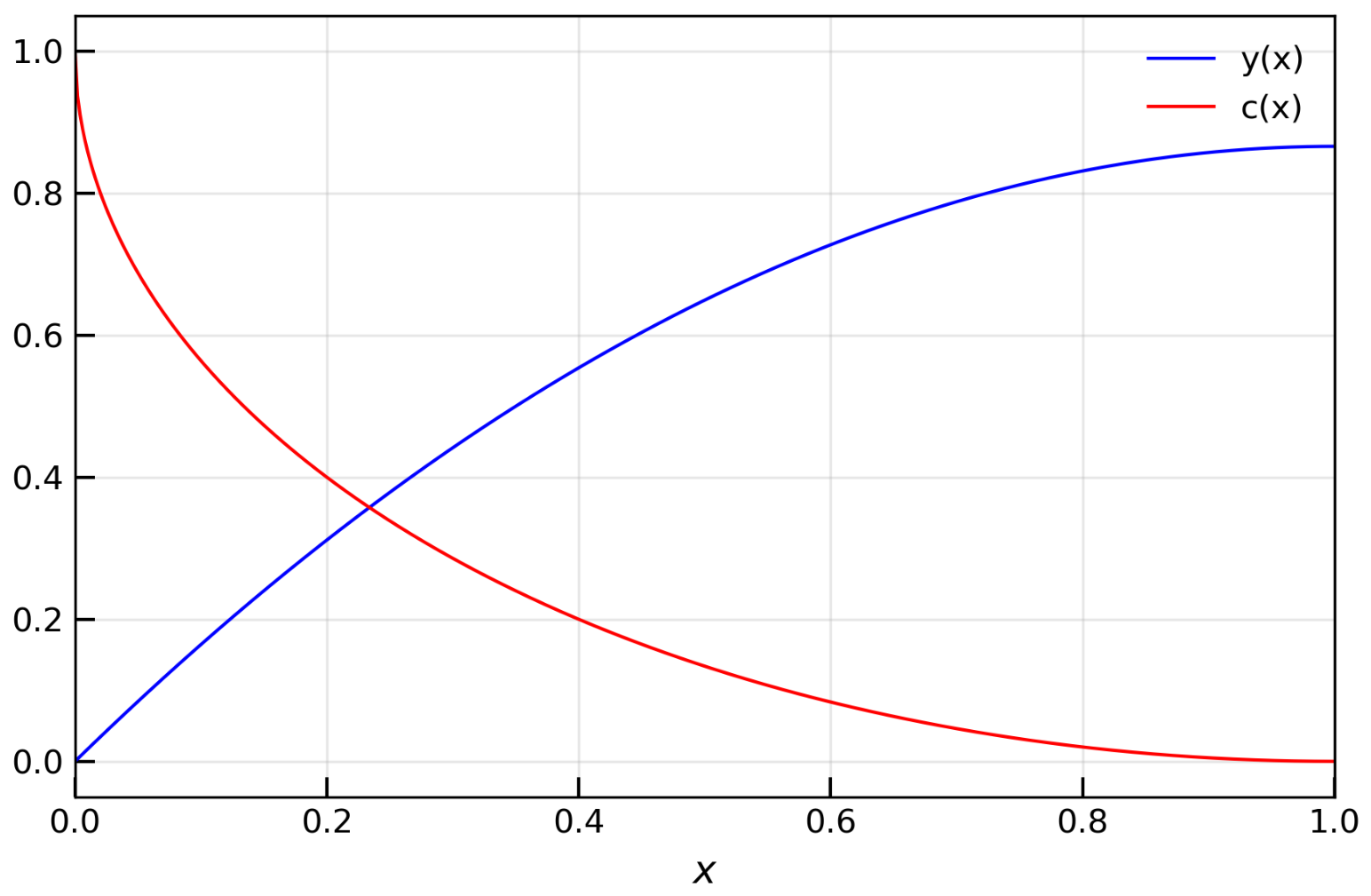
Now, for the fuzzification, $R=2$ is selected, resulting in $x\in [0,1]$, which ensures that y meets the criteria of the increasing generator, where y is a strictly increasing function defined as $y:[0,1]\to \mathbb{R}$, with the condition that $y\left(0\right)=0$. In short,

$$y\left(x\right)=c_{1}x-c_2{x}^2$$

(19)

where $c_1=tan\theta$ and $c_2={\displaystyle \frac{tan\theta }{2}}$ is the increasing generator formed by the fuzzification of the projectile motion under the condition $0^{\circ }$ < $\theta$ < ${90}^{\circ }$, as shown in Figure 6.

Figure 6. The projectile-increasing generator $y\left(x\right)$ is shown at $\theta ={60}^{\circ }$, whereas its complement operator $c\left(x\right)$ is independent of the shape of $y\left(x\right)$.

A more intuitive approach is to view the increasing generator as the height of a projectile. The maximum height H is the value of y at $x=1$, that is, $H=y\left(1\right)$. As $y\left(1\right)={\displaystyle \frac{tan\theta }{2}}$, one can also define the increasing generator in terms of the height function $h\left(x\right)$ as

$$h\left(x\right)=Hx(2-x)$$

(20)

∀$x\in [0,1]$ and $0^{\circ }$ < $\theta$ < ${90}^{\circ }$. Although the increasing generator $h\left(x\right)$ depends on the projection angle, its normalized form h(x)/H is independent of the projection angle.

Proposition 16.

The normalized projectile-increasing generator corresponds to the Schweizer–Sklar increasing generator, while its associated decreasing generator corresponds to Yager’s decreasing generator with a parameter equal to two.

Proof. 

It is straightforward to verify that ${\displaystyle \frac{h\left(x\right)}{H}}=1-{(1-x)}^2$, which corresponds to the Schweizer–Sklar increasing generator with parameter two. The associated decreasing generator is $g\left(x\right)={\displaystyle \frac{h\left(1\right)}{H}}-{\displaystyle \frac{h\left(x\right)}{H}}={(1-x)}^2$, which is Yager’s decreasing generator with a parameter equal to two.    □

4.2. Complement, Intersection and Union Operators

Now we develop the complement, intersection, and union operators from the projectile-increasing generator, utilizing the characterization theorem. The characterization theorem states that an involutive fuzzy complement c, the intersection or t-norm i, and the union or t-conorm u can be derived from a given increasing generator. For $y:[0,1]\to \mathbb{R}$ as an increasing generator and $x_1,x_2\in [0,1]$, we have

$$c\left(x_1\right)=y^{(-1)}(y\left(1\right)-y\left(x_1\right))$$

$$i(x_1,x_2)=y^{(-1)}(y\left(x_1\right)+y\left(x_2\right)-y\left(1\right))$$

$$u(x_1,x_2)=y^{(-1)}(y\left(x_1\right)+y\left(x_2\right))$$

(21)

where $y^{(-1)}$ is a pseudo-inverse of y, which is a function from $\mathbb{R}$ to [0, 1] defined as

$$y^{(-1)}\left(x\right)=\left\{\begin{array}{cc}0,\hfill & \mathrm{if},x\in (-\infty ,0)\hfill \\ y^{-1}\left(x\right),\hfill & \mathrm{if},x\in [0,y(1\left)\right]\hfill \\ 1,\hfill & \mathrm{if},x\in \left(y\right(1),\infty )\hfill \end{array}\right.$$

(22)

and $y^{-1}\left(x\right)$ is the ordinary inverse. For the projectile-increasing generator, $h\left(x\right)=Hx(2-x)$, it is easy to check that the respective complement, intersection, and union operators are as follows.

$$c\left(x\right)=\left\{\begin{array}{cc}0,\hfill & \mathrm{if},H-h\left(x\right)\in (-\infty ,0)\hfill \\ 1-\sqrt{{\displaystyle \frac{h\left(x\right)}{H}}},\hfill & \mathrm{if},H-h\left(x\right)\in [0,H]\hfill \\ 1\hfill & \mathrm{if},H-h\left(x\right)\in (H,\infty )\hfill \end{array}\right.$$

(23)

$$i(x_1,x_2)=\left\{\begin{array}{cc}0,\hfill & \mathrm{if},h\left(x_1\right)+h\left(x_2\right)-H\in (-\infty ,0)\hfill \\ 1-\sqrt{2-({\displaystyle \frac{h\left(x_1\right)}{H}}+{\displaystyle \frac{h\left(x_2\right)}{H}}}),\hfill & \mathrm{if},h\left(x_1\right)+h\left(x_2\right)-H\in [0,H]\hfill \\ 1\hfill & \mathrm{if},h\left(x_1\right)+h\left(x_2\right)-H\in (H,\infty )\hfill \end{array}\right.$$

(24)

$$u(x_1,x_2)=\left\{\begin{array}{cc}0,\hfill & \mathrm{if},h\left(x_1\right)+h\left(x_2\right)\in (-\infty ,0)\hfill \\ 1-\sqrt{1-({\displaystyle \frac{h\left(x_1\right)}{H}}+{\displaystyle \frac{h\left(x_2\right)}{H}}}),\hfill & \mathrm{if},h\left(x_1\right)+h\left(x_2\right)\in [0,H]\hfill \\ 1\hfill & \mathrm{if},h\left(x_1\right)+h\left(x_2\right)\in (H,\infty )\hfill \end{array}\right.$$

(25)

Expressing these operators in terms of $h\left(x\right)$, without explicitly relating them to x, offers several advantages. The first advantage is that $h\left(x\right)$ is normalized by its maximum value H, making these operators independent of the projection angle and the shape of the projectile-increasing generator. The second advantage is that there exists a method to eliminate the “if conditions” from these operators. This is useful as it makes these operators general, independent of their construction by an increasing generator. Since the values of $h\left(x\right)$ vary from 0 to H for the specified $x\in [0,1]$, this consistently constrains the decreasing function $H-h\left(x\right)$ from H to 0, thus allowing for the removal of the “if conditions”, and allowing the complement operator to be rewritten simply as

$$c\left(x\right)=1-\sqrt{{\displaystyle \frac{h\left(x\right)}{H}}}$$

(26)

Similarly, $h\left(x_1\right)$ + $h\left(x_2\right)$ varies from 0 to $2H$, and to remove the “if conditions” from the union and the intersection operators, we simply express them as

$$i(x_1,x_2)=max\left\{0,1-\sqrt{2-({\displaystyle \frac{h\left(x_1\right)}{H}}+{\displaystyle \frac{h\left(x_2\right)}{H}}})\right\}$$

(27)

$$u(x_1,x_2)=real\left\{1-\sqrt{1-({\displaystyle \frac{h\left(x_1\right)}{H}}+{\displaystyle \frac{h\left(x_2\right)}{H}}})\right\}$$

(28)

It is easy to see that these operators form a dual triple $<i,u,c>$ with respect to c (satisfies the De Morgan laws), and hold important properties such as the law of excluded middle ($u(x,c(x\left)\right)=1$) and the law of contradiction ($i(x,c(x\left)\right)=0$). They are rewritten below in standard set notation (removing “real”), and due to normalization, they are also independent of the projection angle.

$$c\left(x\right)=1-\sqrt{1-{(1-x)}^2}$$

(29)

$$i(x_1,x_2)=1-min\left\{1,\sqrt{{(1-x_1)}^2+{(1-x_2)}^2}\right\}$$

(30)

$$u(x_1,x_2)=1-{\left[max\left\{0,{(1-x_1)}^2+{(1-x_2)}^2-1\right\}\right]}^{1/2}$$

(31)

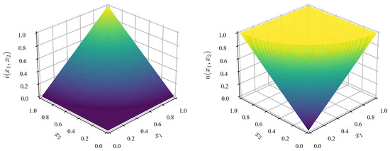
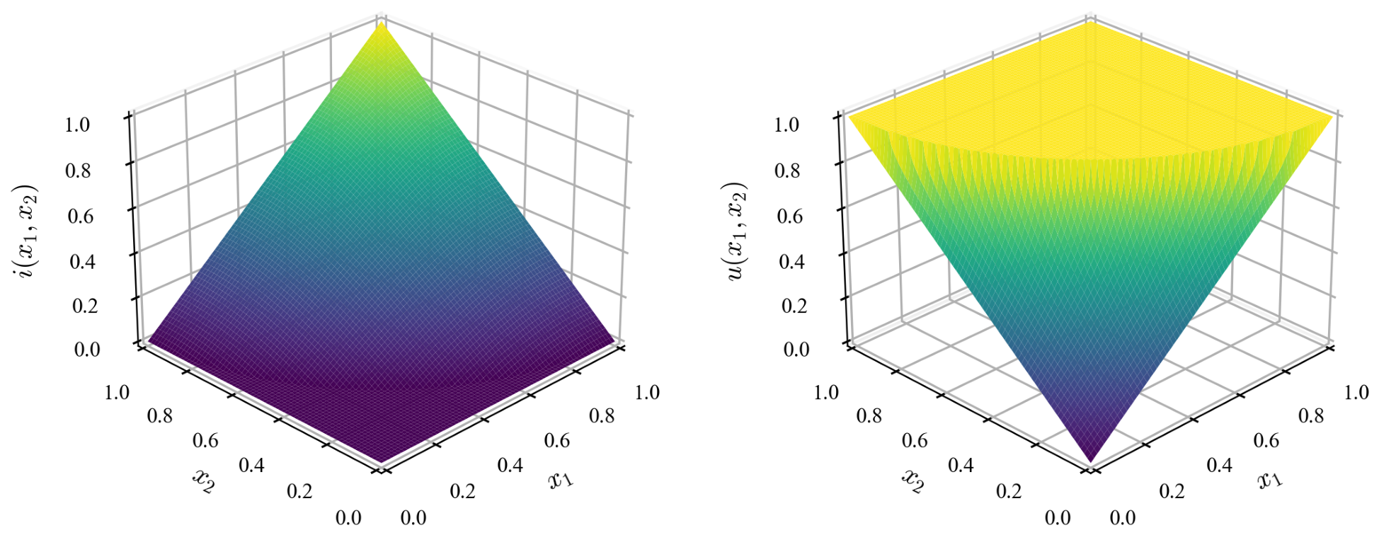
These operators are well-known fuzzy connectives derived directly from the projectile height generator, demonstrating a clear link between classical kinematics and t-norm/t-conorm theory. The derived t-norm operator is a well-established Yager-class of t-norms [57], while complement and t-conorm operators are well-established Schweizer–Sklar classes of fuzzy complements and t-conorms [58]. It is also interesting to observe how the Yager class of t-conorms transforms to the Schweizer–Sklar class of t-conorms when the duality shifts from the standard complement to the projectile complement. This is because the dual complement of a Yager complement is a Schweizer–Sklar complement ($c^d\left(x\right)=1-c(1-x)$). Furthermore, Figure 7 shows arc-like patterns in the t-norm and t-conorm plots, which have a geometric interpretation: for a unit circle centered at $(1,1)$, the t-norm is 0 outside the circle, while the t-conorm is 1 inside it.

Figure 7. Figures showing Yager t-norm ($i(x_1,x_2))$ on the left, and Schweizer–Sklar t-conorm ($u(x_1,x_2))$ on the right, derived from the projectile-increasing generator.

4.3. Equivalence Relation and Metric Space

It is well known that the binary relation $R(X,Y)$ between two crisp sets X and Y of the form $(X\cup \overline{Y})\cap (Y\cup \overline{X})$ is a tautology, where $\overline{X}$ and $\overline{Y}$ are complements of X and Y, respectively. For a fuzzy set concerning a binary relationship with itself, the corresponding expression would be ${\mu }_R(x_i,x_j)=i[u\{\mu \left(x_i\right),c\left(\mu \left(x_j\right)\right)\},u\{c\left(\mu \left(x_i\right)\right),\mu \left(x_j\right)\}]$, ∀$x_i$, $x_j$ ∈ X. The objective is to determine whether ${\mu }_R$ forms a fuzzy equivalence relation under a dual triple, constructed by a projectile-increasing generator. For that, one needs to show the following three properties:

(i)

Reflexivity: ${\mu }_R(x_i,x_j)=1$.

(ii)

Symmetry: ${\mu }_R(x_i,x_j)={\mu }_R(x_j,x_i)$.

(iii)

i − Transitivity: ${\mu }_R(x_i,x_j)={\lambda }_1$ and ${\mu }_R(x_j,x_k)={\lambda }_2$ imply that ${\mu }_R(x_i,x_k)=\lambda$ where $\lambda \ge i[{\lambda }_1,{\lambda }_2]$.

Proposition 17.

A fuzzy relation R on $X^2$ defined as

$${\mu }_R(x_i,x_j)=i[u\{\mu \left(x_i\right),c\left(\mu \left(x_j\right)\right)\},u\left\{c(\mu \left(x_i\right),\mu \left(x_j\right)\}\right]$$

(32)

and constructed under dual triple $<i,u,c>$, generated by a projectile-increasing generator, is a fuzzy $i_P$-equivalence relation for all $x_i$, $x_j$, and $x_k$ in X.

Proof. 

(i) Reflexivity: As $<i,u,c>$ is a dual triple, so $u\{\mu \left(x_i\right),c\left(\mu \left(x_i\right)\right)\}=1$, that is, the law of excluded middle. Thus, ${\mu }_R(x_i,x_i)=1$.

(ii)

Symmetry: As union and intersection operators have the commutative property, it is straightforward to see ${\mu }_R(x_i,x_j)={\mu }_R(x_j,x_i)$.

(iii)

i− Transitivity: At first, let us calculate

$$\begin{array}{cc}\hfill & {\mu }_R(x_i,x_j)=i[u\{\mu \left(x_i\right),c\left(\mu \left(x_j\right)\right)\},u\{c\left(\mu \left(x_i\right)\right),\mu \left(x_j\right)\}]\hfill \\ \hfill & =i[u\{\mu \left(x_i\right),1-\sqrt{1-{(1-\mu \left(x_j\right))}^2}\},u\{1-\sqrt{1-{(1-\mu \left(x_i\right))}^2},\mu \left(x_j\right)\}]\hfill \\ \hfill & =i[real\{1-\sqrt{{(1-\mu \left(x_i\right))}^2-{(1-\mu \left(x_j\right))}^2}\},real\{1-\sqrt{{(1-\mu \left(x_j\right))}^2-{(1-\mu \left(x_i\right))}^2}\}]\hfill \end{array}$$

(33)

For $\mu \left(x_i\right)=\mu \left(x_j\right)$, the result is immediate. For $\mu \left(x_i\right)<\mu \left(x_j\right)$, the term $\sqrt{{(1-\mu \left(x_i\right))}^2-{(1-\mu \left(x_j\right))}^2}$ is real and the term $\sqrt{{(1-\mu \left(x_j\right))}^2-{(1-\mu \left(x_i\right))}^2}$ is imaginary. Using the boundary condition for fuzzy intersection,

$${\mu }_R(x_i,x_j)=max\left\{0,1-\sqrt{{(1-\mu \left(x_i\right))}^2-{(1-\mu \left(x_j\right))}^2}\right\}$$

(34)

Otherwise, for $\mu \left(x_i\right)>\mu \left(x_j\right)$, we have

$${\mu }_R(x_i,x_j)=max\left\{0,1-\sqrt{{(1-\mu \left(x_j\right))}^2-{(1-\mu \left(x_i\right))}^2}\right\}$$

(35)

Combining both cases with absolute value, we conclude that

$${\mu }_R(x_i,x_j)=max\left\{0,1-\sqrt{|{(1-\mu \left(x_i\right))}^2-{(1-\mu \left(x_j\right))}^2|}\right\}$$

(36)

Similarly,

$${\mu }_R(x_j,x_k)=max\left\{0,1-\sqrt{|{(1-\mu \left(x_j\right))}^2-{(1-\mu \left(x_k\right))}^2|}\right\}$$

(37)

This gives

$$\begin{array}{cc}\hfill & i[{\mu }_R(x_i,x_j),{\mu }_R(x_j,x_k)]=\hfill \\ \hfill & max\left\{0,1-\left[\phantom{|{(1-\mu \left(x_j\right))}^2|}|{(1-\mu \left(x_i\right))}^2-{(1-\mu \left(x_j\right))}^2|\right.\right.\hfill \\ \hfill & \left.{\left.+|{(1-\mu \left(x_j\right))}^2-{(1-\mu \left(x_k\right))}^2|\right]}^{1/2}\right\}\hfill \end{array}$$

(38)

or

$$i[{\mu }_R(x_i,x_j),{\mu }_R(x_j,x_k)]\le max\left\{0,1-\sqrt{|{(1-\mu \left(x_i\right))}^2-{(1-\mu \left(x_k\right))}^2|}\right\}$$

(39)

therefore,

$$i[{\mu }_R(x_i,x_j),{\mu }_R(x_j,x_k)]\le {\mu }_R(x_i,x_k)$$

(40)

Hence, ${\mu }_R(x_i,x_j)$ is an $i_P$-equivalence relation, and we denote it by $E_P(x_i,x_j)$.

□

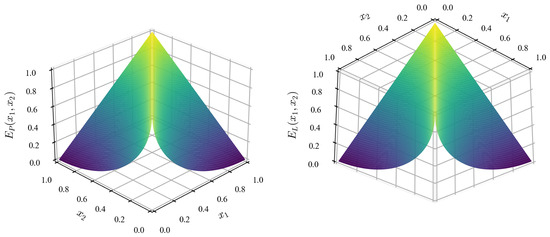
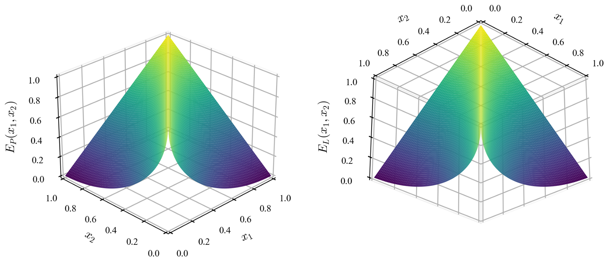
Earlier, we showed that the projectile-increasing generator can be generalized, and consequently so can the t-norm and t-conorm constructed from it. Similarly, $E_P(x_i,x_j)$ can also be generalized, yielding $E_P(x_i,x_j)=1-{\left|{\left(c_s\left(\mu \left(x_i\right)\right)\right)}^r-{\left(c_s\left(\mu \left(x_j\right)\right)\right)}^r\right|}^{1/r},$ where $c_s$ is the standard fuzzy complement, and $r\ge 1$. Different pseudo-metrics can be readily constructed on X with $E_P(x_i,x_j)$, using well-established theorems, such as those of Baets and Mesiar [59] and Bezdek and Harris [60]. These pseudo-metrics on elemental space provide useful techniques for the analysis of fuzzy data. However, obtaining the fuzzy data of a real physical system is often challenging. Therefore, it is advantageous to map the system onto membership space, where these fuzzy techniques can be applied to analyze usual (crisp) data. Furthermore, the generalized projectile equivalence relation can also be viewed as the inverted generalized Łukasiewicz fuzzy equivalence relation [61], which is $E_L(x_i,x_j)=1-{\left|{\left(\mu \left(x_i\right)\right)}^r-{\left(\mu \left(x_j\right)\right)}^r\right|}^{1/r},$ as illustrated in Figure 8.

Figure 8. Figures showing the inverted relation between projectile fuzzy equivalence relation $E_p(x_1,x_2)$, shown on the left, and generalized Łukasiewicz fuzzy equivalence relation $E_L(x_1,x_2)$, shown on the right for $r=2$.

Proposition 18.

Let X be a membership space and $E_P:X^2\to [0,1]$ be a generalized projectile equivalence relation. Then, the distance function constructed from it and defined by $d(\mu \left(x_i\right),\mu \left(x_j\right))=\left|{\left(c_s\left(\mu \left(x_i\right)\right)\right)}^r-{\left(c_s\left(\mu \left(x_j\right)\right)\right)}^r\right|$ is a metric.

Proof. 

There are two methods for the construction. The first approach begins by creating a decreasing generator $f\left(\mu \left(x_i\right)\right)=g\left(1\right)-g\left(\mu \left(x_i\right)\right)$ from the generalized projectile-increasing generator $g\left(\mu \left(x_i\right)\right)=1-{(1-\mu \left(x_i\right))}^r$. Then,

$$d(\mu \left(x_i\right),\mu \left(x_j\right))=f\left(E_P(\mu \left(x_i\right),\mu \left(x_j\right))\right)=\left|{\left(c_s\left(\mu \left(x_i\right)\right)\right)}^r-{\left(c_s\left(\mu \left(x_j\right)\right)\right)}^r\right|$$

It is easy to see that (i) $d(\mu \left(x_i\right),\mu \left(x_j\right))=0$; (ii) $d(\mu \left(x_i\right),\mu \left(x_j\right))=d(\mu \left(x_j\right),\mu \left(x_i\right))$; (iii) triangle inequality holds; and (iv) $d(\mu \left(x_i\right),\mu \left(x_j\right))=0\iff x_i=x_j$, as $E_P(\mu \left(x_i\right),\mu \left(x_j\right))$ is now an equality relation on X. Hence, $d(\mu \left(x_i\right),\mu \left(x_j\right))$ is a metric in X. Later, $d(\mu \left(x_i\right),\mu \left(x_j\right))$ from the membership space can be transformed to the elemental space, $d(x_i,x_j):X^2\to [0,\infty )$, simply by multiplying the required expression by H. The second approach is more straightforward. Since f is a decreasing generator, the distance function constructed from it is simply

$$d(\mu \left(x_i\right),\mu \left(x_j\right))=\left|f\left(\mu \left(x_i\right)\right)-f\left(\mu \left(x_j\right)\right)\right|$$

   □

4.4. Application to Data Clustering

Although data clustering is a vast field, this section focuses on using the projectile fuzzy equivalence relation as a similarity measure for clustering three real datasets: the Iris, cancer, and crude oil datasets. For this process, we use the clustering Algorithm 1 described in Section 2, implemented in MATLAB R2022b scripts. While the algorithm itself remains unchanged, clustering performance depends on the choice of similarity measure and nature of the dataset; this section evaluates the effectiveness of the projectile fuzzy equivalence relation for that purpose, and compares the results with other benchmark similarity measures—Łukasiewicz [61], Euclidean [62], and Jaccard [63]. Next, we will briefly describe the different datasets used in this study.

(a)

Fisher’s Iris dataset [47] includes the classification of three species: Iris setosa, Iris versicolor, and Iris virginica. This classification is achieved by measuring 4 features—sepal length, sepal width, petal length, and petal width—of 150 Iris specimens, with each class containing 50 samples.

(b)

The Breast Cancer Wisconsin (Diagnostic) dataset [48] consists of two classes: 357 malignant samples and 212 benign samples, each defined by 10 features related to the cell nucleus—radius, texture, perimeter, area, smoothness, compactness, concavity, concave points, symmetry, and fractal dimension.

(c)

Gerrild and Lantz conducted a chemical analysis of 56 crude-oil samples [49] taken from three sandstone zones: 7 samples from Wilhelm, 11 from Sub-Mulinia, and the remaining 38 from Upper. The analysis revealed 5 characteristics that include the trace elements’ values for vanadium, iron, beryllium, saturated hydrocarbons, and aromatic hydrocarbons.

Algorithm 1 Clustering algorithm

(i) A decreasing sequence of similarity degrees is chosen, i.e., $1\ge s_1>s_2>\dots >s_r\ge 0$. (ii) For the data $O=\{O_1,\dots ,O_N\}$, we select the similarity degree $s_1=s$ and randomly choose the first sample $O_1=O_0$. (iii) For s and $O_o$, the first cluster is formed according to $C_1=\{0_k,k\in O:{\mu }_{\tilde{R}}(o,k)\ge s\}$. (iv) Then, the remaining sample is put in $O^1$, i.e., $O^1={\displaystyle \frac{O}{C_1}}$. (v) If $O^1\ne \varphi$, then we choose randomly an object $O_v$ with $O_v\notin C_1$ and ${\mu }_R(o,v)=min{O}_1$. (vi) For s and $O_v$, the second cluster is formed according to $C_2=\{O_k,k\in O^1:{\mu }_{\tilde{R}}(v,k)\ge s\}$ (vii) The process is carried out till $C_1$, $C_2$, …, and $C_m$ are formed, such that $O^{m+1}=\varphi$. Then, the clustering algorithm is repeated for another similarity degree and the process goes on till $s_r$.

It is well known that in the Iris dataset, Iris setosa is linearly separable, whereas Iris versicolor and Iris virginica are not; the cancer dataset represents linearly inseparable data, and the crude oil dataset exhibits overlapping data [64].

Since the actual classes of the datasets are known, we choose the external clustering validation index (CVI) to determine the performance of the clustering algorithm in grouping similar data points and separating dissimilar ones. In this scenario, we opt for purity as the external CVI [65,66] to assess the uniformity of clusters in relation to the true classes. Purity is measured as

$$Purity={\displaystyle \frac{1}{n}}{\displaystyle \sum _{i=1}^r}ma{x}_{j=1}^k|C_i\cap G_j|$$

(41)

where $|C_i\cap G_j|$ is the number of data points that are common to cluster $C_i$ and class $G_j$, and n is the total number of data points.

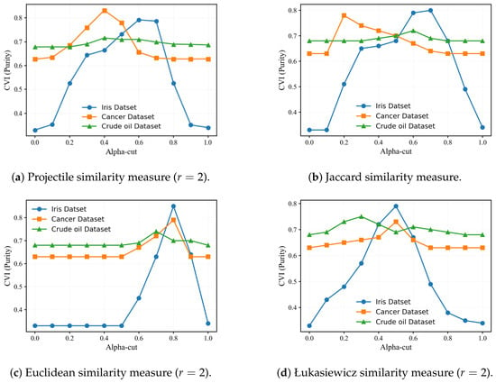
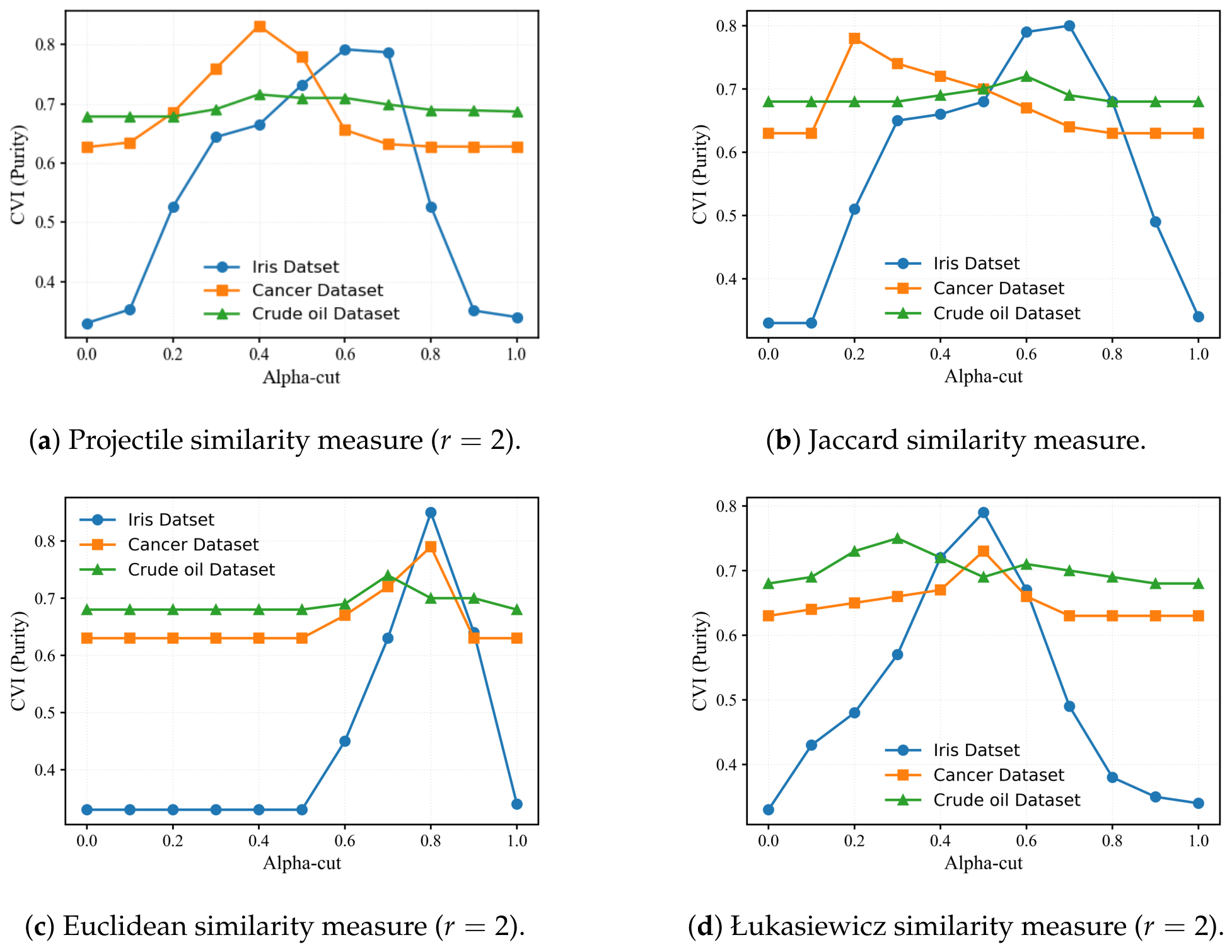
After 30 repeated runs, the outcomes of the clustering analysis are illustrated in Figure 9. The Euclidean similarity measure is a distance-based measure, so the clusters remain unchanged until the gap between two data points exceeds the threshold. Consequently, purity increases sharply after the $\alpha$-cut exceeds 0.5. In contrast, the Jaccard similarity measure is a set-theoretic measure and sensitive to position rather than gap, resulting in a more continuous variation in purity. Although the Łukasiewicz similarity measure is fundamentally distance-based, it distorts this behavior for $r>1$; unlike the Euclidean similarity measure, it does not exhibit a flat region below the threshold. Interestingly, the CVI of the Projectile similarity measure indicates behavior closer to that of a set-theoretic measure.

Figure 9. Clustering results using (a) Projectile, (b) Jaccard, (c) Euclidean, and (d) Łukasiewicz fuzzy equivalence relations as similarity measures.

For the Iris dataset, the CVI of the Projectile and Jaccard similarity measures reaches its peak with a plateau observed over the alpha interval [0.6, 0.7], suggesting that strong clusters exist at these similarity levels. However, the absence of the peak with a plateau in the CVI of the Euclidean and Łukasiewicz similarity measure suggests that despite the linearly separable classes of the Iris dataset, their clustering results are fragile. On the other hand, the clustering outcomes resulting from all four similarity measure for the cancer dataset and the crude oil dataset are more or less the same. This suggests that predicting the structure of these datasets can yield plausible results. In the context of the cancer dataset, there exists a unique point where the CVI reaches its peak, and both preceding and following this point, there is a gradual decline in similarity, suggesting the absence of a clearly defined equivalence structure or overlapping data points, and the clusters are not stable, meaning they change rapidly with alpha. Finally, the flat curve the in crude oil dataset shows the insensitivity of the CVI to the similarity threshold or alpha-cut, or the dataset has no well-defined similarity scale. The insensitivity occurs as two of the three classes are considerably smaller when compared to the third class, resulting in a single dominant cluster for all similarity thresholds.

5. Conclusions

In this paper, we have thoroughly explored the development of the PFN through the fuzzification of projectile motion equation. The transformation of a PFN from the $(a,b)$ notation to the $(m,tan\theta )$ notation significantly enhances its arithmetic operations. It has been demonstrated that both the standard alpha-cut method and the approximation method yield identical PFNs after addition or subtraction. However, in the case of multiplication or division, the approximation method retains the shape, whereas the standard alpha-cut method might not generate the PFN. Moreover, this study also establishes a fuzzy equivalence relation derived from the fuzzification of projectile motion equation. Initially, the increasing generator is created, and by utilizing the characterization theorem, the associated t-norm and t-conorm are formulated. It is noteworthy that the so produced t-norm aligns with the Yager class of t-norms, with a parameter set to two, while the t-conorm corresponds to the Schweizer–Sklar class of t-conorms, also with a parameter of two, and these two are dual with respect to the constructed complement operator. By extending the concept of tautology, a projectile fuzzy equivalence relation is established. Furthermore, it is demonstrated that the dissimilarity relation derived from this projectile fuzzy equivalence relation qualifies as a metric in the membership space. Finally, the projectile fuzzy equivalence relation is used for fuzzy data clustering of the Iris, cancer, and crude oil datasets, and the results show remarkable accuracy. It is believed that this study can further be utilized in modeling uncertainty in real-world situations, data analysis, decision-making processes, and various scientific challenges.

References

- Klir, G.J. Developments in Uncertainty-Based Information. In Advances in Computers; Elsevier: Amsterdam, The Netherlands, 1993; Volume 36, pp. 255–332. [Google Scholar] [CrossRef] [Scilit]
- Öztürk, F. Some Conceptual and Measurement Aspects of Complexity, Chaos, and Randomness from Mathematical Point of View; Springer: Cham, Switzerland, 2018; pp. 33–66. [Google Scholar] [CrossRef] [Scilit]
- Solomatine, D.; Solomatine, D.; Kuzmin, V.; Shrestha, D.L. Learning Errors of Environmental Mathematical Models; Springer: Berlin/Heidelberg, Germany, 2013; pp. 466–473. [Google Scholar] [CrossRef] [Scilit]
- Brugnach, M.; Pahl-Wostl, C.; Lindenschmidt, K.; Janssen, J.; Filatova, T.; Mouton, A.; Holtz, G.; van der Keur, P.; Gaber, N. Complexity and Uncertainty: Rethinking the Modelling Activity; Elsevier: Amsterdam, The Netherlands, 2008; Volume 3, pp. 49–68. [Google Scholar] [CrossRef] [Scilit]
- Takai, S. A use of a mathematical model in updating concept selection. J. Mech. Des. 2010, 132, 101009. [Google Scholar] [CrossRef] [Scilit]
- Gardashova, L.A. Modeling of Decision Maker Under Imperfect Information. In Recent Developments and New Direction in Soft-Computing Foundations and Applications: Selected Papers from the 4th World Conference on Soft Computing, Berkeley, CA, USA, 25–27 May 2014; Zadeh, L.A., Abbasov, A.M., Yager, R.R., Shahbazova, S.N., Reformat, M.Z., Eds.; Springer International Publishing: Cham, Switzerland, 2016; pp. 503–513. [Google Scholar] [CrossRef] [Scilit]
- Aliev, R.A.; Huseynov, O.H. Decision Theory with Imperfect Information; World Scientific: Singapore, 2014. [Google Scholar] [CrossRef] [Scilit]
- Klir, G.J. Where do we stand on measures of uncertainty, ambiguity, fuzziness, and the like? Fuzzy Sets Syst. 1987, 24, 141–160. [Google Scholar] [CrossRef] [Scilit]
- Barhoumi, S.; Kallel, I.K.; Bouhamed, S.A.; Bosse, E.; Solaiman, B. Generation of fuzzy evidence numbers for the evaluation of uncertainty measures. In International Conference on Advanced Technologies for Signal and Image Processing; IEEE: New York, NY, USA, 2020; pp. 1–6. [Google Scholar] [CrossRef] [Scilit]
- Sander, W. Uncertainty and Fuzziness; Vieweg+Teubner Verlag: Wiesbaden, Germany, 1994; pp. 265–273. [Google Scholar] [CrossRef] [Scilit]
- Zadeh, L.A.; Fu, K.S.; Tanaka, K.; Shimura, M. Fuzzy Sets and Their Applications to Cognitive and Decision Processes; Academic Press: Cambridge, MA, USA, 2008. [Google Scholar]
- Auger, A.; Roy, J. Expression of uncertainty in linguistic data. In International Conference on Information Fusion; IEEE: New York, NY, USA, 2008; pp. 1–8. [Google Scholar]
- Carey, J.M.; Burgman, M.A. Linguistic Uncertainty in Qualitative Risk Analysis and How to Minimize It. Ann. N. Y. Acad. Sci. 2008, 1128, 13–17. [Google Scholar] [CrossRef] [Scilit] [PubMed]
- Ferrero, A.; Salicone, S. Measurement uncertainty. IEEE Instrum. Meas. Mag. 2006, 9, 44–51. [Google Scholar] [CrossRef] [Scilit]
- Ebrahimnejad, A.; Verdegay, J.L. Fuzzy Set Theory; Springer: Cham, Switzerland, 2018; pp. 1–27. [Google Scholar] [CrossRef] [Scilit]
- Bandemer, H. Fuzzy Specification of Uncertain Knowledge and Vague or Imprecise Information; Springer: Vienna, Austria, 1995; pp. 1–21. [Google Scholar] [CrossRef] [Scilit]
- Zadeh, L. Fuzzy sets. Inf. Control 1965, 8, 338–353. [Google Scholar] [CrossRef] [Scilit]
- Zimmermann, H.J. Fuzzy set theory. WIREs Comput. Stat. 2010, 2, 317–332. [Google Scholar] [CrossRef] [Scilit]
- de Barros, L.C.; Bassanezi, R.C.; Lodwick, W.A. The Extension Principle of Zadeh and Fuzzy Numbers; Springer Nature: Berlin, Germany, 2024; pp. 23–42. [Google Scholar] [CrossRef] [Scilit]
- Zadeh, L. The concept of a linguistic variable and its application to approximate reasoning—I. Inf. Sci. 1975, 8, 199–249. [Google Scholar] [CrossRef] [Scilit]
- Zadeh, L. Similarity relations and fuzzy orderings. Inf. Sci. 1971, 3, 177–200. [Google Scholar] [CrossRef] [Scilit]
- Fodor, J.; Yager, R.R. Fuzzy Set-Theoretic Operators and Quantifiers; Springer: Boston, MA, USA, 2000; pp. 125–193. [Google Scholar] [CrossRef] [Scilit]
- Garrido, A. Triangular Norms, Triangular Conorms, and Some Related Concepts. BRAIN Broad Res. Artif. Intell. Neurosci. 2011, 2, 59–62. [Google Scholar]
- Kechagias, P.; Papadopoulos, B.K. Computational method to evaluate fuzzy arithmetic operations. Appl. Math. Comput. 2007, 185, 169–177. [Google Scholar] [CrossRef] [Scilit]
- Jia, Y.; Wang, Z. Application of artificial intelligence based on the fuzzy control algorithm in enterprise innovation. Heliyon 2024, 10, e28116. [Google Scholar] [CrossRef] [Scilit] [PubMed]
- Chang, W.; Park, J.B.; Joo, Y.H.; Chen, G. Design of sampled-data fuzzy-model-based control systems by using intelligent digital redesign. IEEE Trans. Circuits Syst. I Fundam. Theory Appl. 2002, 49, 509–517. [Google Scholar] [CrossRef]
- Wierzchoń, S. Applications of fuzzy decision-making theory to coping with ill-defined problems. Fuzzy Sets Syst. 1982, 7, 1–18. [Google Scholar] [CrossRef] [Scilit]
- Capocelli, R.; De Luca, A. Fuzzy sets and decision theory. Inf. Control 1973, 23, 446–473. [Google Scholar] [CrossRef] [Scilit]
- Pappis, C.P.; Karacapilidis, N.I. Application of a similarity measure of fuzzy sets to fuzzy relational equations. Fuzzy Sets Syst. 1995, 75, 135–142. [Google Scholar] [CrossRef] [Scilit]
- Hai, N.T.; Chosa, T.; Tojo, S.; Thi-Hien, N. Application of a Similarity Measure Using Fuzzy Sets to Select the Optimal Plan for an Air-Assisted Rice Seeder. Appl. Sci. 2021, 11, 6715. [Google Scholar] [CrossRef] [Scilit]
- Cao, J.; Zhou, T.; Zhi, S.; Lam, S.; Ren, G.; Zhang, Y.; Wang, Y.; Dong, Y.; Cai, J. Fuzzy inference system with interpretable fuzzy rules: Advancing explainable artificial intelligence for disease diagnosis—A comprehensive review. Inf. Sci. 2024, 662, 120212. [Google Scholar] [CrossRef] [Scilit]
- Shoaip, N.; El-Sappagh, S.; AbuHmed, T.; Elmogy, M. A dynamic fuzzy rule-based inference system using fuzzy inference with semantic reasoning. Sci. Rep. 2024, 14, 4275. [Google Scholar] [CrossRef] [Scilit] [PubMed]
- Adil, O.; Ali, M.; Ali, A.Y.; Sumait, B.S. Comparison between the Effects of Different Types of Membership Functions on Fuzzy Logic Controller Performance. Int. J. Emerg. Eng. Res. Technol. 2015, 3, 76–83. [Google Scholar]
- Gupta, S.; Biswas, P.K.; Aljafari, B.; Thanikanti, S.B.; Das, S.K. Modelling, simulation and performance comparison of different membership functions based fuzzy logic control for an active magnetic bearing system. J. Eng. 2023, 2023, e12229. [Google Scholar] [CrossRef] [Scilit]
- Nahmias, S. Fuzzy variables. Fuzzy Sets Syst. 1978, 1, 97–110. [Google Scholar] [CrossRef] [Scilit]
- Dubois, D.; Prade, H. Operations on fuzzy numbers. Int. J. Syst. Sci. 1978, 9, 613–626. [Google Scholar] [CrossRef] [Scilit]
- Bohlender, G.; Kaufmann, A.; Gupta, M.M. Introduction to Fuzzy Arithmetic, Theory and Applications. Math. Comput. 1986, 47, 762. [Google Scholar] [CrossRef] [Scilit]
- Moore, R.; Lodwick, W. Interval analysis and fuzzy set theory. Fuzzy Sets Syst. 2003, 135, 5–9. [Google Scholar] [CrossRef] [Scilit]
- Kaufmann, A.; Gupta, M.M. Introduction to Fuzzy Arithmetic: Theory and Applications; Van Nostrand Reinhold Co.: New York, NY, USA, 1985. [Google Scholar]
- Jager, R.; Verbruggen, H.; Bruijn, P. The Role of Defuzzification Methods in the Application of Fuzzy Control. IFAC Proc. Vol. 1992, 25, 75–80. [Google Scholar] [CrossRef] [Scilit]
- Leekwijck, W.V.; Kerre, E.E. Defuzzification: Criteria and classification. Fuzzy Sets Syst. 1999, 108, 159–178. [Google Scholar] [CrossRef] [Scilit]
- Pedrycz, W. Why triangular membership functions? Fuzzy Sets Syst. 1994, 64, 21–30. [Google Scholar] [CrossRef] [Scilit]
- Sen, S.; Patra, K.; Mondal, S. Similarity Measure of Gaussian Fuzzy Numbers and Its Application. Int. J. Appl. Comput. Math. 2021, 7, 96. [Google Scholar] [CrossRef] [Scilit]
- Zadeh, L.A. Fuzzy Sets and Their Application to Pattern Classification and Clustering Analysis. In Classification and Clustering; Academic Press: New York, NY, USA; San Francisco, CA, USA; London, UK, 1977; pp. 355–393. [Google Scholar] [CrossRef] [Scilit]
- Bezdek, J.C.; Pal, S.K. Fuzzy Models for Pattern Recognition; USDOE Pittsburgh Energy Technology Center: Pittsburgh, PA, USA; Oregon State University: Corvallis, OR, USA; IEEE Press: New York, NY, USA; Naval Research Laboratory: Washington, DC, USA; Electric Power Research Institute: Palo Alto, CA, USA; Bureau of Mines: Washington, DC, USA, 1994. [Google Scholar]
- Menger, K. Probabilistic Theories of Relations. Proc. Natl. Acad. Sci. USA 1951, 37, 178–180. [Google Scholar] [CrossRef] [Scilit] [PubMed]
- Fisher, R. The use of multiple measurements in taxonomic problems. Ann. Eugen. 1936, 2, 179–188. [Google Scholar] [CrossRef] [Scilit]
- Wolberg, W.; Mangasarian, O.; Street, N.; Street, W. Breast Cancer Wisconsin (Diagnostic) [Data Set]. UCI Machine Learning Repository. Available online: https://archive.ics.uci.edu/dataset/17/breast+cancer+wisconsin+diagnostic (accessed on 20 September 2026).
- Gerrild, P.; Lantz, R. Chemical Analysis of 75 Crude Oil Samples from Pliocene Sand Units, Elk Hills Oil Field, California; Technical Report; U.S. Geological Survey: Reston, VA, USA, 1969. [CrossRef] [Scilit]
- Klir, G.J.; Yuan, B. Fuzzy Sets and Fuzzy Logic: Theory and Applications; Prentice Hall: Upper Saddle River, NJ, USA, 1995. [Google Scholar]
- Zimmermann, H.J. Fuzzy Set Theory and Its Applications Third Edition; Kluwer Academic Publishers: Boston, MA, USA; Dordrecht, The Netherlands; London, UK, 1996. [Google Scholar]
- Bandemer, H.; NÄther, W. Fuzzy Data Analysis; Springer: Dordrecht, The Netherlands, 1992. [Google Scholar]
- Didier, D.; Prade, H.M. Fundamentals of Fuzzy Sets; Kluwer Academic Publishers: Boston, MA, USA; Dordrecht, The Netherlands; London, UK, 2000. [Google Scholar]
- Wadsworth, F.B.; Vasseur, J.; Foster, A.; Smith, A.P.W.; Byatt, N.A.; Allgood, C.; Loisel, A.; Bintang, F.; Squirrell, D.; Paine, A.; et al. Projectile motion: Experimental datasets and classroom exercises. Phys. Educ. 2025, 60, 045024. [Google Scholar] [CrossRef] [Scilit]
- Asma, A.F.; Priya, G. Optimizing Triangular Parabolic Fuzzy EOQ Model with Shortage Using Nearest Interval Approximation. Int. J. Future Revolut. Comput. Sci. Commun. Eng. 2017, 3, 92–96. [Google Scholar]
- Garg, H.; Ansha. Arithmetic Operations on Generalized Parabolic Fuzzy Numbers and Its Application. Proc. Natl. Acad. Sci. India Sect. A Phys. Sci. 2018, 88, 15–26. [Google Scholar] [CrossRef] [Scilit]
- Yager, R.R. On a general class of fuzzy connectives. Fuzzy Sets Syst. 1980, 4, 235–242. [Google Scholar] [CrossRef] [Scilit]
- Schweizer, B.; Sklar, A. Associative functions and abstract semigroups. Publ. Math. Debr. 1963, 10, 9–81. [Google Scholar] [CrossRef] [Scilit]
- De Baets, B.; Mesiar, R. Pseudo-metrics and T-equivalences. J. Fuzzy Math. 1997, 5, 471–481. [Google Scholar]
- Bezdek James, C.; Harris Douglas, J. Fuzzy partitions and relations; an axiomatic basis for clustering. Fuzzy Sets Syst. 1978, 1, 111–127. [Google Scholar] [CrossRef] [Scilit]
- Luukka, P.; Saastamoinen, K.; Kononen, V. A classifier based on the maximal fuzzy similarity in the generalized Lukasiewicz-structure. In Proceedings of the 10th IEEE International Conference on Fuzzy Systems, (Cat. No.01CH37297), Melbourne, VIC, Australia, 2–5 December 2001; IEEE: New York, NY, USA, 2001; Volume 1, pp. 195–198. [Google Scholar] [CrossRef] [Scilit]
- Levy, A.; Shalom, B.R.; Chalamish, M. A Guide to Similarity Measures. arXiv 2024, arXiv:2408.07706. [Google Scholar] [CrossRef] [Scilit]
- McCulloch, J.; Wagner, C.; Aickelin, U. Analysing Fuzzy Sets Through Combining Measures of Similarity and Distance. In IEEE International Conference on Fuzzy Systems; IEEE: New York, NY, USA, 2014. [Google Scholar] [CrossRef] [Scilit][Green Version]
- Pakhira, M.K.; Bandyopadhyay, S.; Maulik, U. A study of some fuzzy cluster validity indices, genetic clustering and application to pixel classification. Fuzzy Sets Syst. 2005, 155, 191–214. [Google Scholar] [CrossRef] [Scilit]
- Rendón, E.; Abundez, I.; Arizmendi, A.; Quiroz, E. Internal versus external cluster validation indexes. Int. J. Comput. Commun. 2011, 5, 27–34. [Google Scholar]
- Zerabi, S.; Meshoul, S.; Merniz, A.; Melal, R. Towards Clustering Validation in Big Data Context. In Proceedings of the 2nd International Conference on Big Data, Cloud and Applications, BDCA’17, New York, NY, USA, 29–30 March 2017. [Google Scholar] [CrossRef] [Scilit]
Disclaimer/Publisher’s Note: The statements, opinions and data contained in all publications are solely those of the individual author(s) and contributor(s) and not of MDPI and/or the editor(s). MDPI and/or the editor(s) disclaim responsibility for any injury to people or property resulting from any ideas, methods, instructions or products referred to in the content. |
© 2026 by the author. Licensee MDPI, Basel, Switzerland. This article is an open access article distributed under the terms and conditions of the Creative Commons Attribution (CC BY) license.