Stability and Hopf Bifurcation with Optimal Control in a Delayed Tripartite Evolutionary Game

Abstract

This paper studies new energy adoption using a tripartite evolutionary game involving government incentives, enterprise investment, and user adoption. Two time delays are introduced to describe delayed enterprise responses to policy incentives and delayed user perceptions of supply improvements, while social feedback captures interactions among users. The equilibria and their local stability are analyzed, and Hopf bifurcation conditions are derived for the single-delay and double-delay cases. Numerical results illustrate that, under representative parameter settings, both types of delays can induce a loss of local stability of the interior equilibrium and lead to oscillatory behavior near the corresponding critical delays. Social feedback also plays an important role in determining system stability. Finally, an optimal control model based on Pontryagin’s maximum principle is developed for the delay-free benchmark system to promote the transition from low to high adoption while accounting for intervention costs. The results highlight the effects of delayed responses, social feedback, and policy control on the evolutionary dynamics of new energy adoption.

1. Introduction

The low-carbon transition of energy systems is a complex evolutionary process shaped by interactions among technological development, policy intervention, market response, user behavior, and social feedback [1,2]. As new energy technologies are increasingly being adopted in power generation, energy storage, transportation, and end-use sectors, their diffusion exhibits typical features of complex dynamical systems, including multi-agent interactions, nonlinear feedback, delayed responses, and path dependence [3,4]. These characteristics make new energy adoption more than a static decision problem and motivate the development of dynamical models capable of describing its long-term evolution, stability, and possible regime transitions [5,6].

Evolutionary game theory provides a natural framework for describing adaptive decision making among boundedly rational agents [7,8,9,10]. In new energy adoption, the government, energy enterprises, and end users constitute three interacting populations with distinct strategic objectives. The government adjusts incentives and regulatory measures, enterprises decide whether to invest in and supply new energy technologies, and users determine whether to adopt the corresponding products or services [11,12]. Their decisions depend on relative payoffs and continuously affect one another, leading to coupled replicator dynamics. Compared with static game-theoretic approaches, evolutionary dynamics can capture the adjustment of strategy proportions over time and reveal how collective behavior emerges from repeated interactions among heterogeneous populations [13,14]. New energy adoption can therefore be regarded as a nonlinear coevolutionary process involving multiple boundedly rational groups [15,16,17].

An important source of complexity in this process is delayed response. Policy signals generally do not affect enterprise decisions immediately because policy implementation, project approval, financing, and technology deployment require time [18,19,20,21]. Similarly, users may respond to changes in product quality, service availability, and supporting infrastructure only after a perception and adaptation period. Such delays create temporal mismatches between policy intervention, supply adjustment, and demand response. When incorporated into evolutionary dynamics, they transform the system into a delayed nonlinear dynamical system whose stability is governed by the roots of transcendental characteristic equations [22,23]. Time delay can qualitatively change the dynamical behavior of nonlinear systems. As the delay passes through a critical value, a locally stable equilibrium may lose stability, and oscillatory behavior may emerge through a local Hopf bifurcation under the corresponding spectral and transversality conditions [24,25]. In the context of new energy adoption, these oscillations may correspond to repeated adjustments among policy incentives, enterprise investment, and user adoption caused by delayed information and behavioral responses [26,27]. Identifying the associated critical delay therefore provides a dynamical criterion for determining when gradual adaptation may turn into endogenous fluctuations [28,29,30]. Social feedback further modifies this evolutionary process. The expansion of digital platforms, social networks, and information channels has strengthened interactions among users and made adoption decisions increasingly dependent on collective behavior [31,32,33,34,35]. A higher adoption level may generate positive feedback through demonstration effects, social learning, and word-of-mouth diffusion. By contrast, congestion, insufficient infrastructure, declining service quality, or weakened incentives may generate negative feedback as adoption increases. Hence, depending on its direction and magnitude, social feedback may either reinforce diffusion or contribute to the stabilization of the adoption dynamics. Its interaction with delayed responses can therefore produce dynamical outcomes that cannot be inferred from either mechanism alone.

Existing studies have investigated green technology diffusion and new energy promotion using evolutionary games, system dynamics, complex networks, and multi-agent approaches [36,37]. However, several issues remain insufficiently explored. First, many evolutionary-game models emphasize bilateral interactions, such as government–enterprise, enterprise–consumer, or government–consumer games, whereas the coupled evolution of government intervention, enterprise investment, and user adoption deserves further dynamical analysis. Second, policy response delay and user perception delay are often examined separately, while their combined effects on stability and oscillatory behavior remain less understood. Third, social feedback may substantially alter the stability properties of the system, but its interaction with multiple delays has received limited attention. Finally, stability and bifurcation analyses identify when undesirable fluctuations arise, but they do not directly determine how policy interventions should be adjusted over time while accounting for intervention costs [38,39,40]. Motivated by these issues, we develop a tripartite delayed evolutionary game model for the coupled evolution of government incentives, enterprise investment, and user adoption. The main contributions are threefold. First, a three-population evolutionary dynamic system is formulated in which government, enterprise, and user strategies evolve endogenously and are coupled through payoff feedback. Social feedback associated with user adoption is explicitly incorporated into the behavioral dynamics. Second, two distinct delay mechanisms, representing the enterprise response to government policy and the user response to enterprise supply, are introduced. The equilibria and their local stability are analyzed, and the conditions under which increasing delays induce stability loss and Hopf bifurcation are investigated. Third, an optimal control problem is formulated to examine time-dependent intervention strategies that promote new energy adoption while accounting for the associated policy costs. The theoretical analysis is complemented by numerical simulations illustrating equilibrium transitions, delay-induced oscillations, and controlled evolutionary trajectories.

The remainder of this paper is organized as follows. Section 2 formulates the tripartite delayed evolutionary game model and derives the corresponding replicator dynamics. Section 3 examines the equilibria and their local stability and analyzes delay-induced Hopf bifurcations. Section 4 formulates the optimal control problem and derives the associated optimality conditions. Section 5 presents numerical simulations to illustrate the theoretical results and explore the effects of key parameters. Finally, Section 6 summarizes the main conclusions.

2. Model Construction

The government strategy set is denoted by $G=\{G_1,G_2\}$. Here, $G_1$ represents active incentives, such as subsidies, tax incentives, green credit, infrastructure construction, and strict regulation. $G_2$ represents passive regulation, in which the government only maintains basic market regulation. The strategy set of energy enterprises is denoted by $E=\{E_1,E_2\}$. Here, $E_1$ represents investing in new energy, such as wind energy, solar energy, energy storage, hydrogen energy, and related green technologies. $E_2$ represents maintaining traditional energy operations, such as coal, oil, and natural gas businesses. The strategy set of end users is denoted by $U=\{U_1,U_2\}$. Here, $U_1$ represents adopting new energy, such as purchasing new energy vehicles, installing distributed photovoltaics, using green electricity, or using energy-saving equipment. $U_2$ represents not adopting new energy and continuing to use traditional energy products. To describe the dynamic process of new energy promotion, two delays are considered. The enterprise response delay ${\tau }_1\ge 0$ reflects the time needed for government policies to affect enterprise investment. The user perception delay ${\tau }_2\ge 0$ reflects the time needed for users to perceive improvements in product supply, service networks, and market reputation. Let $x\left(t\right)\in [0,1]$ denote the proportion of governments choosing active incentives at time t, $y\left(t\right)\in [0,1]$ denote the proportion of enterprises investing in new energy, and $z\left(t\right)\in [0,1]$ denote the proportion of users adopting new energy. The main parameters are given in Table 1. Based on the practical process of new energy adoption, the following assumptions are proposed.

Table 1. Model parameters.

Parameter	Meaning	Range
M	Government benefit from promoting new energy transition	$M\ge 0$
$C_g$	Cost of government incentives	$C_g\ge 0$
$S_g$	Subsidy for enterprises investing in new energy	$S_g\ge 0$
$S_u$	Subsidy for users adopting new energy	$S_u\ge 0$
L	Penalty on enterprises maintaining traditional energy operations	$L\ge 0$
$R_e$	Return from new energy investment	$R_e>0$
$C_e$	Cost of new energy investment	$C_e\ge 0$
$R_t$	Return from traditional energy operations	$R_t\ge 0$
P	Market return of new energy products	$P\ge 0$
$B_u$	Green utility from adopting new energy	$B_u\ge 0$
$C_u$	Additional cost of adopting new energy	$C_u\ge 0$
T	Additional traditional-energy use cost or carbon-related cost under active government regulation	$T\ge 0$
$\eta$	Market expansion benefit from user adoption	$\eta \ge 0$
$\theta$	User utility improvement from enterprise investment	$\theta \ge 0$
D	Loss of traditional energy demand due to new energy adoption	$D\ge 0$
$\beta$	Social feedback coefficient	$\beta \in \mathbb{R}$
k	Average degree of the user network	$k>0$
$z_c$	Threshold of social feedback	$0<z_c<1$
${\tau }_1$	Enterprise response delay to policy incentives	${\tau }_1\ge 0$
${\tau }_2$	User perception delay of enterprise supply improvement	${\tau }_2\ge 0$

Assumption 1.

The participants include the government, energy enterprises, and end users, all of whom are boundedly rational. The government chooses between active incentives and passive regulation. Energy enterprises choose between investing in new energy and maintaining traditional energy operations. End users choose between adopting and not adopting new energy. The three agents adjust their strategies gradually according to payoff changes.

Assumption 2.

If the government adopts active incentives, it obtains the long-term performance benefit M but bears the incentive cost $C_g$. It provides subsidies $S_g$ to enterprises investing in new energy and subsidies $S_u$ to users adopting new energy. It can also impose a penalty L on enterprises maintaining traditional energy operations. If the government adopts passive regulation, it does not provide additional subsidies or penalties.

Assumption 3.

If energy enterprises invest in new energy, they obtain the basic return $R_e$ and bear the investment cost $C_e$. They can receive the government subsidy $S_g$ under active incentives. If users adopt new energy, enterprises obtain the product market return P and the market expansion benefit η. If enterprises maintain traditional energy operations, they obtain the traditional return $R_t$ but may suffer the penalty L under active government regulation. In addition, the expansion of new energy adoption reduces traditional energy demand, and the corresponding loss is denoted by D.

Assumption 4.

If end users adopt new energy, they obtain green utility $B_u$ but bear the adoption cost $C_u$ and pay the product price P. Under active government incentives, they receive the subsidy $S_u$. If enterprises invest in new energy, users obtain additional utility θ due to improvements in supply, technology, and services. If users do not adopt new energy, they may bear an additional traditional-energy use cost or carbon-related cost T under active government regulation; under passive regulation, this additional policy-induced cost is not imposed. User adoption is also affected by social feedback, which is characterized by the average network degree k, the social feedback coefficient β, and the diffusion threshold $z_c$.

Assumption 5.

Time delays exist in the new energy adoption process. The response of enterprises to government policies has a delay ${\tau }_1$, so current enterprise investment may be affected by past policy incentives. Users’ perception of enterprise supply improvement also has a delay ${\tau }_2$, so current user adoption may be affected by past enterprise investment.

Based on these assumptions, the payoff matrix is shown in Table 2. Each cell lists the payoffs of the government, energy enterprise, and end user in order. Table 2 gives the basic payoff structure under pure strategies. In the replicator dynamic model, the social feedback effect is written as $\beta k[z\left(t\right)-z_c]$, which reflects the influence of imitation, demonstration, and word-of-mouth effects on user adoption. It should be noted that Table 2 reports the payoffs under pure population strategy profiles. Hence, under the pure adoption strategy $U_1$, $z=1$ and the general social-feedback term $\beta k[z\left(t\right)-z_c]$ reduces to $\beta k(1-z_c)$. In the subsequent replicator dynamics, $z\left(t\right)\in [0,1]$ varies endogenously, and the general frequency-dependent form is therefore retained. To describe time delays, $x(t-{\tau }_1)$ is introduced into the enterprise payoff function, and $y(t-{\tau }_2)$ is introduced into the user payoff function. Thus, a delayed multi-agent evolutionary game system is obtained.

Table 2. Payoff matrix of the tripartite game among the government, energy enterprises, and end users.

Government Strategy	Enterprise Strategy	User Adopts New Energy ${\mathit{U}}_1$	User Does Not Adopt New Energy ${\mathit{U}}_2$
$G_1$	$E_1$	$\left(M-C_g-S_g-S_u,R_e-C_e+S_g+P+\eta ,B_u-C_u-P+S_u+\theta +\beta k(1-z_c)\right)$	$\left(M-C_g-S_g,R_e-C_e+S_g,-T\right)$
	$E_2$	$\left(M-C_g-S_u+L,R_t-L-D,B_u-C_u-P+S_u+\beta k(1-z_c)\right)$	$\left(M-C_g+L,R_t-L,-T\right)$
$G_2$	$E_1$	$\left(0,R_e-C_e+P+\eta ,B_u-C_u-P+\theta +\beta k(1-z_c)\right)$	$\left(0,R_e-C_e,0\right)$
	$E_2$	$\left(0,R_t-D,B_u-C_u-P+\beta k(1-z_c)\right)$	$\left(0,R_t,0\right)$

For the government, the payoff difference between active incentives and passive regulation is

$${\Delta }_G=M+L-C_g-(S_g+L)y\left(t\right)-S_{u}z\left(t\right).$$

(1)

where $M+L-C_g$ represents the basic net benefit of active incentives. The term $-(S_g+L)y\left(t\right)$ indicates that, when more enterprises invest in new energy, the government needs to provide more subsidies and receives less penalty revenue. The term $-S_{u}z\left(t\right)$ represents the subsidy cost caused by user adoption.

For energy enterprises, the payoff difference between investing in new energy and maintaining traditional energy operations is

$${\Delta }_E=R_e-C_e-R_t+(S_g+L)x(t-{\tau }_1)+(\eta +P+D)z\left(t\right).$$

(2)

where $R_e-C_e-R_t$ is the basic payoff difference between new energy investment and traditional energy operations. The term $(S_g+L)x(t-{\tau }_1)$ represents the delayed effect of government incentives and penalties. The term $(\eta +P+D)z\left(t\right)$ shows that user adoption increases market demand and improves the return from new energy investment.

For end users, the payoff difference between adopting and not adopting new energy is

$${\Delta }_U=B_u-C_u-P+(S_u+T)x\left(t\right)+\theta y(t-{\tau }_2)+\beta k[z\left(t\right)-z_c].$$

(3)

where $B_u-C_u-P$ is the basic net utility of adopting new energy. The term $(S_u+T)x\left(t\right)$ represents the effect of government subsidies and traditional energy costs. The term $\theta y(t-{\tau }_2)$ describes the delayed effect of enterprise investment on user adoption. The term $\beta k[z\left(t\right)-z_c]$ captures threshold-dependent social feedback. When $\beta >0$, deviations from the threshold $z_c$ are reinforced, adoption is discouraged when $z<z_c$ and encouraged when $z>z_c$. When $\beta <0$, the feedback is stabilizing, increasing adoption incentives below the threshold and reducing them above the threshold.

Thus, the tripartite delayed evolutionary game system is obtained as

$$\left\{\begin{array}{cc}\hfill \dot{x}\left(t\right)& =x\left(t\right)(1-x\left(t\right)){\Delta }_G\hfill \\ & =x\left(t\right)(1-x\left(t\right))[M+L-C_g-(S_g+L)y\left(t\right)-S_{u}z\left(t\right)],\hfill \\ \hfill \dot{y}\left(t\right)& =y\left(t\right)(1-y\left(t\right)){\Delta }_E\hfill \\ & =y\left(t\right)(1-y\left(t\right))[R_e-C_e-R_t+(S_g+L)x(t-{\tau }_1)+(\eta +P+D)z\left(t\right)]\hfill \\ \hfill \dot{z}\left(t\right)& =z\left(t\right)(1-z\left(t\right)){\Delta }_U\hfill \\ & =z\left(t\right)(1-z\left(t\right))[B_u-C_u-P+(S_u+T)x\left(t\right)+\theta y(t-{\tau }_2)+\beta k(z\left(t\right)-z_c)].\hfill \end{array}\right.$$

(4)

3. Equilibrium and Hopf Bifurcation Analysis

3.1. Stability Analysis

According to Equation (4), an equilibrium satisfies $x(1-x){\Delta }_G=0$, $y(1-y){\Delta }_E=0$, $z(1-z){\Delta }_U=0$. Since an equilibrium is time-independent, the delayed variables satisfy $x(t-{\tau }_1)=x$ and $y(t-{\tau }_2)=y$ at equilibrium. Therefore, the time delays do not affect the locations of the equilibria. When all three populations adopt pure strategies, the system has eight corner equilibria, namely $E_1=(0,0,0)$, $E_2=(1,0,0)$, $E_3=(0,1,0)$, $E_4=(0,0,1)$, $E_5=(1,1,0)$, $E_6=(1,0,1)$, $E_7=(0,1,1)$, and $E_8=(1,1,1)$. In addition to these corner equilibria, the system may admit partially mixed equilibria on the faces and edges of the strategy space ${[0,1]}^3$. On the face $z=0$, for example, a partially mixed equilibrium with $0<x<1$ and $0<y<1$ is $E_{z=0}^m=\left(-{\displaystyle \frac{R_e-C_e-R_t}{S_g+L}},{\displaystyle \frac{M+L-C_g}{S_g+L}},0\right)$, provided that the first two coordinates lie in $(0,1)$. Similarly, on the face $z=1$, the partially mixed equilibrium is $E_{z=1}^m=\left(-{\displaystyle \frac{R_e-C_e-R_t+\eta +P+D}{S_g+L}},{\displaystyle \frac{M+L-C_g-S_u}{S_g+L}},1\right)$, provided that the first two coordinates lie in $(0,1)$. On the faces $y=0$ and $y=1$, respectively, the partially mixed equilibria are $E_{y=0}^m=\left(-{\displaystyle \frac{B_u-C_u-P+\beta k\left(\frac{M+L-C_g}{S_u}-z_c\right)}{S_u+T}},0,{\displaystyle \frac{M+L-C_g}{S_u}}\right)$, and $E_{y=1}^m=\left(-{\displaystyle \frac{B_u-C_u-P+\theta +\beta k\left(\frac{M-C_g-S_g}{S_u}-z_c\right)}{S_u+T}},1,{\displaystyle \frac{M-C_g-S_g}{S_u}}\right)$, provided that the two non-boundary coordinates lie in $(0,1)$. Likewise, on the faces $x=0$ and $x=1$, the partially mixed equilibria are $E_{x=0}^m=\left(0,-{\displaystyle \frac{B_u-C_u-P+\beta k\left(-\frac{R_e-C_e-R_t}{\eta +P+D}-z_c\right)}{\theta }},-{\displaystyle \frac{R_e-C_e-R_t}{\eta +P+D}}\right)$, and $E_{x=1}^m=\left(1,-{\displaystyle \frac{B_u-C_u-P+S_u+T+\beta k\left(-\frac{R_e-C_e-R_t+S_g+L}{\eta +P+D}-z_c\right)}{\theta }},-{\displaystyle \frac{R_e-C_e-R_t+S_g+L}{\eta +P+D}}\right)$, again provided that the two non-boundary coordinates lie in $(0,1)$ and the corresponding denominators are nonzero. Partially mixed equilibria may also occur on the edges with $x=i$, $y=j$, and $0<z<1$, where $i,j\in \{0,1\}$. They can be written as $E_{ij}^z=\left(i,j,z_c-{\displaystyle \frac{B_u-C_u-P+(S_u+T)i+\theta j}{\beta k}}\right),i,j\in \{0,1\}$, provided that $\beta \ne 0$ and the third coordinate lies in $(0,1)$. For edges on which only x or only y is mixed, isolated mixed equilibria do not generally occur because ${\Delta }_G$ is independent of x and ${\Delta }_E$ is independent of y. Under special parameter equalities, however, continua of edge equilibria may arise.

Although Equation (4) contains the delayed variables $x(t-{\tau }_1)$ and $y(t-{\tau }_2)$, the delay terms do not affect the first-order local stability of the eight corner equilibria. Specifically, the coefficients associated with the delayed perturbations are proportional to $y^{*}(1-y^{*})$ and $z^{*}(1-z^{*})$, respectively. Since $y^{*},z^{*}\in \{0,1\}$ at each corner equilibrium, these coefficients vanish. Therefore, the local linearization at the eight corner equilibria is independent of ${\tau }_1$ and ${\tau }_2$ and coincides with that of the corresponding delay-free system. Hence, the following matrix can be used to determine their local stability:

$$J=\left(\begin{array}{ccc}(1-2x)A& -x(1-x)(S_g+L)& -x(1-x)S_u\\ y(1-y)(S_g+L)& (1-2y)B& y(1-y)(\eta +P+D)\\ z(1-z)(S_u+T)& \theta z(1-z)& (1-2z)C+z(1-z)\beta k\end{array}\right).$$

(5)

where $A=M+L-C_g-(S_g+L)y-S_{u}z$, $B=R_e-C_e-R_t+(S_g+L)x+(\eta +P+D)z$, and $C=B_u-C_u-P+(S_u+T)x+\theta y+\beta k(z-z_c)$. The local stability conditions of the eight corner equilibria are summarized in Table 3. It should be emphasized that Equation (5) is used here only for the local stability analysis of these eight pure-strategy corner equilibria. At these equilibria, the coefficients associated with the delayed perturbations vanish, so the first-order local linearization is independent of ${\tau }_1$ and ${\tau }_2$. For partially mixed and fully interior equilibria, however, the delayed terms generally do not vanish and must be retained in the corresponding linearization. The full delay-dependent linearization of the interior equilibrium is considered subsequently.

Table 3. Stability conditions of the eight corner equilibria.

Equilibrium	Local Asymptotic Stability Conditions
$E_1=(0,0,0)$	$M+L<C_g,R_e-C_e-R_t<0,B_u-C_u-P<\beta k{z}_c$
$E_2=(1,0,0)$	$M+L>C_g,R_e-C_e-R_t+S_g+L<0,B_u-C_u-P+S_u+T<\beta k{z}_c$
$E_3=(0,1,0)$	$M<C_g+S_g,R_e-C_e-R_t>0,B_u-C_u-P+\theta <\beta k{z}_c$
$E_4=(0,0,1)$	$M+L<C_g+S_u,R_e-C_e-R_t+\eta +P+D<0,B_u-C_u-P+\beta k(1-z_c)>0$
$E_5=(1,1,0)$	$M>C_g+S_g,R_e-C_e-R_t+S_g+L>0,B_u-C_u-P+S_u+T+\theta <\beta k{z}_c$
$E_6=(1,0,1)$	$M+L>C_g+S_u,R_e-C_e-R_t+S_g+L+\eta +P+D<0,B_u-C_u-P+S_u+T+\beta k(1-z_c)>0$
$E_7=(0,1,1)$	$M<C_g+S_g+S_u,R_e-C_e-R_t+\eta +P+D>0,B_u-C_u-P+\theta +\beta k(1-z_c)>0$
$E_8=(1,1,1)$	$M>C_g+S_g+S_u,R_e+S_g+L+\eta +P+D>C_e+R_t,B_u+S_u+T+\theta +\beta k(1-z_c)>C_u+P$

In addition to boundary equilibria, the system may also have an internal equilibrium point $E^{*}=(x^{*},y^{*},z^{*})$, satisfying $0<x^{*},y^{*},z^{*}<1$. Therefore, the internal equilibrium point satisfies the following system of equations:

$$\left\{\begin{array}{c}M+L-C_g-(S_g+L)y^{*}-S_u{z}^{*}=0,\hfill \\ R_e-C_e-R_t+(S_g+L)x^{*}+(\eta +P+D)z^{*}=0,\hfill \\ B_u-C_u-P+(S_u+T)x^{*}+\theta y^{*}+\beta k(z^{*}-z_c)=0.\hfill \end{array}\right.$$

(6)

Solving Equation (6) yields the interior mixed equilibrium $E^{*}=(x^{*},y^{*},z^{*})$, where $z^{*}={\displaystyle \frac{(S_g+L)\left[\beta k{z}_c-(B_u-C_u-P)\right]+(S_u+T)(R_e-C_e-R_t)-\theta (M+L-C_g)}{(S_g+L)\beta k-(S_u+T)(\eta +P+D)-\theta S_u}}$, $y^{*}={\displaystyle \frac{M+L-C_g-S_u{z}^{*}}{S_g+L}}$, and $x^{*}={\displaystyle \frac{-(R_e-C_e-R_t)-(\eta +P+D)z^{*}}{S_g+L}}$. For the interior equilibrium to be well defined, the denominators must be nonzero; that is, $(S_g+L)\beta k-(S_u+T)(\eta +P+D)-\theta S_u\ne 0$, and $S_g+L\ne 0$. Moreover, for $E^{*}$ to be economically meaningful and to lie in the interior of the strategy space, it must satisfy $0<x^{*}<1$, $0<y^{*}<1$, $0<z^{*}<1$.

Let $u\left(t\right)=x\left(t\right)-x^{*}$, $v\left(t\right)=y\left(t\right)-y^{*}$, $w\left(t\right)=z\left(t\right)-z^{*}$, where $u\left(t\right)$, $v\left(t\right)$, and $w\left(t\right)$ denote small perturbations of the system state variables around the internal equilibrium point. Denote $m_1=x^{*}(1-x^{*})$, $m_2=y^{*}(1-y^{*})$, $m_3=z^{*}(1-z^{*})$, since $0<x^{*},y^{*},z^{*}<1$, we have $m_1>0$, $m_2>0$, and $m_3>0$. From Equation (4), the linearized system near $E^{*}$ is given by

$$\left\{\begin{array}{c}\dot{u}\left(t\right)=-m_1(S_g+L)v\left(t\right)-m_1{S}_{u}w\left(t\right),\hfill \\ \dot{v}\left(t\right)=m_2(S_g+L)u(t-{\tau }_1)+m_2(\eta +P+D)w\left(t\right),\hfill \\ \dot{w}\left(t\right)=m_3(S_u+T)u\left(t\right)+m_3\theta v(t-{\tau }_2)+m_3\beta kw\left(t\right).\hfill \end{array}\right.$$

(7)

Assume that the perturbation solution takes the exponential form ${(u\left(t\right),v\left(t\right),w\left(t\right))}^T={(U,V,W)}^T{e}^{\lambda t}$, where $\lambda$ is the characteristic root. Therefore, the characteristic equation corresponding to the internal mixed equilibrium point can be written as follows:

$$det\left(\begin{array}{ccc}\lambda & m_1(S_g+L)& m_1{S}_u\\ -m_2(S_g+L)e^{-\lambda {\tau }_1}& \lambda & -m_2(\eta +P+D)\\ -m_3(S_u+T)& -m_3\theta e^{-\lambda {\tau }_2}& \lambda -m_3\beta k\end{array}\right)=0.$$

(8)

To obtain a relatively explicit stability criterion, we first consider the delay-free case, namely ${\tau }_1=0$ and ${\tau }_2=0$. In this case, the characteristic equation Equation (8) degenerates into a third-order polynomial equation. The characteristic equation in the delay-free case can be written as

$${\lambda }^3+a_1{\lambda }^2+a_2\lambda +a_3=0.$$

(9)

where $a_3=-m_1{m}_2{m}_3{(S_g+L)}^2\beta k+m_1{m}_2{m}_3{S}_u(S_g+L)\theta +m_1{m}_2{m}_3(S_g+L)(\eta +P+D)(S_u+T)$, $a_2=m_1{m}_2{(S_g+L)}^2+m_1{m}_3{S}_u(S_u+T)-m_2{m}_3(\eta +P+D)\theta$ and $a_1=-m_3\beta k$.

According to the Routh–Hurwitz criterion, the interior equilibrium is locally asymptotically stable in the delay-free case if $a_1>0$, $a_2>0$, $a_3>0$, and $a_1{a}_2>a_3$. Since $m_3>0$ and $k>0$, the condition $a_1=-m_3\beta k>0$ requires $\beta <0$. Therefore, negative social feedback is a necessary condition for local asymptotic stability of the interior equilibrium, but it is not sufficient by itself, because the remaining Routh–Hurwitz conditions must also be satisfied. Conversely, if $\beta >0$, then $a_1<0$, and the Routh–Hurwitz conditions cannot all hold.

3.2. Hopf Bifurcation

Three delay scenarios are considered, including the enterprise response delay to policy incentives, the user perception delay of enterprise supply improvement, and the simultaneous existence of both delays. For notational simplicity, let ${\varphi }_1=S_g+L$, ${\varphi }_2=S_u$, ${\varphi }_3=S_u+T$, ${\varphi }_4=\eta +P+D$, ${\varphi }_5=\theta$.

3.2.1. Response Delay of Enterprises to Policy Incentives

When only the response delay of enterprises to policy incentives is considered, let ${\tau }_1=\tau$ and ${\tau }_2=0$. In this case, the corresponding characteristic equation Equation (8) can be written as

$$P_1\left(\lambda \right)+Q_1\left(\lambda \right)e^{-\lambda \tau }=0.$$

(10)

where $P_1\left(\lambda \right)={\lambda }^3+a_1{\lambda }^2+a_2\lambda +a_3$, $Q_1\left(\lambda \right)=b_1\lambda +b_0$, with $a_1=-m_3\beta k$, $a_2=m_1{m}_3{\varphi }_2{\varphi }_3-m_2{m}_3{\varphi }_4{\varphi }_5$, $a_3=m_1{m}_2{m}_3{\varphi }_1{\varphi }_3{\varphi }_4$, $b_1=m_1{m}_2{\varphi }_1^2$, and $b_0=-m_1{m}_2{m}_3\beta k{\varphi }_1^2+m_1{m}_2{m}_3{\varphi }_1{\varphi }_2{\varphi }_5$.

Let $\lambda =i\omega$, where $\omega >0$; substituting it into Equation (10) gives

$$P_1\left(i\omega \right)+Q_1\left(i\omega \right)e^{-i\omega \tau }=0.$$

(11)

From the modulus equality condition, we obtain $|P_1\left(i\omega \right)|=|Q_1\left(i\omega \right)|$. Since $P_1\left(i\omega \right)=(a_3-a_1{\omega }^2)+i(a_2\omega -{\omega }^3)$, and $Q_1\left(i\omega \right)=b_0+i{b}_1\omega$, $\omega$ satisfies

$${\omega }^6+(a_1^2-2a_2){\omega }^4+(a_2^2-2a_1{a}_3-b_1^2){\omega }^2+(a_3^2-b_0^2)=0.$$

(12)

If Equation (12) has positive roots ${\omega }_k$, then the corresponding critical delays are given by

$${\tau }_{k,j}^{\left(1\right)}={\displaystyle \frac{1}{{\omega }_k}}\left[arg{Q}_1\left(i{\omega }_k\right)-arg[-P_1\left(i{\omega }_k\right)]+2j\pi \right],k=1,2,\dots ,j=0,1,2,\dots .$$

(13)

The first positive critical delay is defined as ${\tau }_0^{\left(1\right)}=min\{{\tau }_{k,j}^{\left(1\right)}>0\}$. Assume that the interior equilibrium $E^{*}$ is locally asymptotically stable at $\tau =0$, and that at $\tau ={\tau }_0^{\left(1\right)}$ the characteristic equation has a simple pair of purely imaginary roots $\lambda =\pm i{\omega }_0$, while all the remaining characteristic roots have negative real parts. If, in addition, the transversality condition ${\left.{\displaystyle \frac{dRe\left(\lambda \right)}{d\tau }}\right|}_{\tau ={\tau }_0^{\left(1\right)}}\ne 0$ holds, then the pair of characteristic roots crosses the imaginary axis with nonzero speed, and a local Hopf bifurcation occurs near $\tau ={\tau }_0^{\left(1\right)}$. This result indicates that the enterprise response delay may affect the local stability of the system. For $0\le \tau <{\tau }_0^{\left(1\right)}$, the interior equilibrium remains locally asymptotically stable under the above spectral assumptions. As $\tau$ passes through ${\tau }_0^{\left(1\right)}$, the equilibrium may lose stability and oscillatory behavior may emerge through a local Hopf bifurcation. This conclusion is local to the critical delay and does not imply that the equilibrium remains unstable for all larger values of $\tau$, since additional stability switches may occur.

3.2.2. Perception Delay of Users Regarding Enterprise Supply Improvement

When only the perception delay of users regarding improvements in enterprise supply is considered, let ${\tau }_1=0$ and ${\tau }_2=\tau$. In this case, the characteristic equation Equation (8) can be written as

$$P_2\left(\lambda \right)+Q_2\left(\lambda \right)e^{-\lambda \tau }=0.$$

(14)

where $P_2\left(\lambda \right)={\lambda }^3+{\tilde{a}}_1{\lambda }^2+{\tilde{a}}_2\lambda +{\tilde{a}}_3$, $Q_2\left(\lambda \right)={\tilde{b}}_1\lambda +{\tilde{b}}_0$, with ${\tilde{a}}_1=-m_3\beta k$, ${\tilde{a}}_2=m_1{m}_2{\varphi }_1^2+m_1{m}_3{\varphi }_2{\varphi }_3$, ${\tilde{a}}_3=-m_1{m}_2{m}_3\beta k{\varphi }_1^2+m_1{m}_2{m}_3{\varphi }_1{\varphi }_3{\varphi }_4$, ${\tilde{b}}_1=-m_2{m}_3{\varphi }_4{\varphi }_5$, and ${\tilde{b}}_0=m_1{m}_2{m}_3{\varphi }_1{\varphi }_2{\varphi }_5$.

Let $\lambda =i\omega$, where $\omega >0$. Substituting it into Equation (14) gives

$$P_2\left(i\omega \right)+Q_2\left(i\omega \right)e^{-i\omega \tau }=0.$$

(15)

From the modulus equality condition, we obtain $|P_2\left(i\omega \right)|=|Q_2\left(i\omega \right)|$. Since $P_2\left(i\omega \right)=({\tilde{a}}_3-{\tilde{a}}_1{\omega }^2)+i({\tilde{a}}_2\omega -{\omega }^3)$, and $Q_2\left(i\omega \right)={\tilde{b}}_0+i{\tilde{b}}_1\omega$, $\omega$ satisfies

$${\omega }^6+({\tilde{a}}_1^2-2{\tilde{a}}_2){\omega }^4+({\tilde{a}}_2^2-2{\tilde{a}}_1{\tilde{a}}_3-{\tilde{b}}_1^2){\omega }^2+({\tilde{a}}_3^2-{\tilde{b}}_0^2)=0.$$

(16)

If Equation (16) has positive roots ${\omega }_k$, then the corresponding critical delays are given by

$${\tau }_{k,j}^{\left(2\right)}={\displaystyle \frac{1}{{\omega }_k}}\left[arg{Q}_2\left(i{\omega }_k\right)-arg[-P_2\left(i{\omega }_k\right)]+2j\pi \right],k=1,2,\dots ,j=0,1,2,\dots .$$

(17)

The first positive critical delay is defined as ${\tau }_0^{\left(2\right)}=min\{{\tau }_{k,j}^{\left(2\right)}>0\}$. Assume that the interior equilibrium $E^{*}$ is locally asymptotically stable at $\tau =0$, and that at $\tau ={\tau }_0^{\left(2\right)}$ the characteristic equation has a simple pair of purely imaginary roots $\lambda =\pm i{\omega }_0$, while all the remaining characteristic roots have negative real parts. If, in addition, the transversality condition ${\left.{\displaystyle \frac{dRe\left(\lambda \right)}{d\tau }}\right|}_{\tau ={\tau }_0^{\left(2\right)}}\ne 0$ holds, then the pair of characteristic roots crosses the imaginary axis with nonzero speed, and a local Hopf bifurcation occurs near $\tau ={\tau }_0^{\left(2\right)}$. This conclusion is local to the critical delay and does not imply that the equilibrium remains unstable for all larger values of $\tau$.

3.2.3. Policy Response Delay and User Perception Delay

When the policy response delay and the user perception delay are considered simultaneously, the characteristic equation Equation (8) contains the delay terms $e^{-\lambda {\tau }_1}$ and $e^{-\lambda {\tau }_2}$, as well as the coupled term $e^{-\lambda ({\tau }_1+{\tau }_2)}$. After simplification, the characteristic equation Equation (8) can be written as

$$P_0\left(\lambda \right)+P_1\left(\lambda \right)e^{-\lambda {\tau }_1}+P_2\left(\lambda \right)e^{-\lambda {\tau }_2}+P_{12}{e}^{-\lambda ({\tau }_1+{\tau }_2)}=0.$$

(18)

where $P_0\left(\lambda \right)={\lambda }^3+c_1{\lambda }^2+c_2\lambda +c_3$, $P_1\left(\lambda \right)=d_1\lambda +d_0$, $P_2\left(\lambda \right)=e_1\lambda +e_0$, and $P_{12}=r_0$. The corresponding coefficients are given by $c_1=-m_3\beta k$, $c_2=m_1{m}_3{S}_u(S_u+T)$, $c_3=m_1{m}_2{m}_3(S_g+L)(\eta +P+D)(S_u+T)$, $d_1=m_1{m}_2{(S_g+L)}^2$, $d_0=-m_1{m}_2{m}_3\beta k{(S_g+L)}^2$, $e_1=-m_2{m}_3(\eta +P+D)\theta$, $e_0=0$, and $r_0=m_1{m}_2{m}_3(S_g+L)S_u\theta$.

Different from the single-delay cases, Equation (18) is a double-delay transcendental characteristic equation whose roots are jointly affected by ${\tau }_1$ and ${\tau }_2$. Because of the coupling term $e^{-\lambda ({\tau }_1+{\tau }_2)}$, the double-delay system cannot, in general, be characterized by a single critical delay. Instead, candidate imaginary-root loci may arise in the $({\tau }_1,{\tau }_2)$ plane. These loci identify parameter combinations at which the characteristic equation may admit purely imaginary roots and hence provide candidate points for changes in local stability or Hopf bifurcation. To determine such candidate loci, let $\lambda =i\omega$ with $\omega >0$. Substituting it into Equation (18) yields

$$P_0\left(i\omega \right)+P_1\left(i\omega \right)e^{-i\omega {\tau }_1}+P_2\left(i\omega \right)e^{-i\omega {\tau }_2}+r_0{e}^{-i\omega ({\tau }_1+{\tau }_2)}=0.$$

(19)

where $P_0\left(i\omega \right)=(c_3-c_1{\omega }^2)+i(c_2\omega -{\omega }^3)$, $P_1\left(i\omega \right)=d_0+i{d}_1\omega$, and $P_2\left(i\omega \right)=e_0+i{e}_1\omega$. Expanding the exponential terms into trigonometric form, we have $e^{-i\omega {\tau }_1}=cos\left(\omega {\tau }_1\right)-isin\left(\omega {\tau }_1\right)$, $e^{-i\omega {\tau }_2}=cos\left(\omega {\tau }_2\right)-isin\left(\omega {\tau }_2\right)$, and $e^{-i\omega ({\tau }_1+{\tau }_2)}=cos\left[\omega ({\tau }_1+{\tau }_2)\right]-isin\left[\omega ({\tau }_1+{\tau }_2)\right]$.

Separating the real and imaginary parts of Equation (19), we obtain

$$c_3-c_1{\omega }^2+d_{0}cos\left(\omega {\tau }_1\right)+d_1\omega sin\left(\omega {\tau }_1\right)+e_1\omega sin\left(\omega {\tau }_2\right)+r_{0}cos\left[\omega ({\tau }_1+{\tau }_2)\right]=0,$$

(20)

and

$$c_2\omega -{\omega }^3+d_1\omega cos\left(\omega {\tau }_1\right)-d_{0}sin\left(\omega {\tau }_1\right)+e_1\omega cos\left(\omega {\tau }_2\right)-r_{0}sin\left[\omega ({\tau }_1+{\tau }_2)\right]=0.$$

(21)

The parameter pairs satisfying Equations (20) and (21) define an imaginary-root locus in the $({\tau }_1,{\tau }_2)$ plane, which can be written as $\mathcal{C}=\{({\tau }_1,{\tau }_2):\lambda =\pm i\omega ,\omega >0\}$. This locus identifies candidate parameter values at which the characteristic equation admits a pair of purely imaginary roots. However, $\mathcal{C}$ should not be interpreted automatically as the actual stability boundary of the double-delay system. At a candidate point $({\tau }_1^0,{\tau }_2^0)\in \mathcal{C}$, suppose that the characteristic equation has a simple pair of purely imaginary roots $\lambda =\pm i{\omega }_0$, while no other characteristic roots lie on the imaginary axis. If, in addition, the transversality condition ${\left.{\displaystyle \frac{dRe\left(\lambda \right)}{ds}}\right|}_{s=s_0}\ne 0$ holds, where s denotes a path parameter crossing the locus $\mathcal{C}$, then the corresponding characteristic roots cross the imaginary axis with nonzero speed, and a local Hopf bifurcation may occur near $({\tau }_1^0,{\tau }_2^0)$. Therefore, Equations (20) and (21) provide candidate Hopf points in the double-delay parameter plane, but they do not by themselves determine the complete stable and unstable regions. A change in local stability can occur only at points on $\mathcal{C}$ that also satisfy the relevant spectral and transversality conditions. Determining the complete stability regions would require additional analysis of the characteristic roots on both sides of the imaginary-root locus.

4. Optimal Control Model

Since the optimal control problem of delayed systems is relatively complex, this section uses a delay-free benchmark model, namely ${\tau }_1={\tau }_2=0$. This setting means that policy transmission and user perception are assumed to be relatively timely. In the process of new energy promotion, the government can regulate the system through supply-side and demand-side policies. Supply-side policies encourage enterprises to invest in new energy through subsidies, tax incentives, and green credit. Demand-side policies encourage users to adopt new energy through consumption subsidies, price discounts, and reward mechanisms. Accordingly, three control variables are introduced. Let $u_0\left(t\right)$ denote the intensity of green governance or institutional promotion, which increases the payoff of active government incentives. Let $u_1\left(t\right)$ denote the intensity of enterprise investment subsidies. Let $u_2\left(t\right)$ denote the intensity of user adoption incentives. These controls satisfy $0\le u_0\left(t\right)\le u_0^{max}$, $0\le u_1\left(t\right)\le u_1^{max}$, $0\le u_2\left(t\right)\le u_2^{max}$. After introducing these control variables, the controlled state system can be written as

$$\left\{\begin{array}{c}\dot{x}=x(1-x)\left[M+L-C_g+u_0-(S_g+L+u_1)y-(S_u+u_2)z\right],\hfill \\ \dot{y}=y(1-y)\left[R_e-C_e-R_t+(S_g+L+u_1)x+(\eta +P+D)z\right],\hfill \\ \dot{z}=z(1-z)\left[B_u-C_u-P+(S_u+T+u_2)x+\theta y+\beta k(z-z_c)\right].\hfill \end{array}\right.$$

(22)

Equation (22) shows that the green governance assessment intensity $u_0\left(t\right)$ can increase the relative payoff of the government adopting the active incentive strategy. The enterprise investment subsidy $u_1\left(t\right)$ increases the government’s incentive cost on the one hand and enhances enterprises’ motivation to invest in new energy on the other hand. The user adoption incentive $u_2\left(t\right)$ increases government subsidy expenditure on the one hand, and improves the relative payoff of users adopting new energy on the other hand. Therefore, a dynamically coupled mechanism with state-dependent characteristics is formed among government regulation, enterprise investment, and user adoption.

We seek to steer the system state toward the desired target state $(x_d,y_d,z_d)$. To this end, the following trajectory-tracking optimal control objective functional is formulated:

$$\begin{array}{cc}\hfill maxJ=& -{\int }_0^{T_f}\left[{\displaystyle \frac{Q_1}{2}}{(x-x_d)}^2+{\displaystyle \frac{Q_2}{2}}{(y-y_d)}^2+{\displaystyle \frac{Q_3}{2}}{(z-z_d)}^2+{\displaystyle \frac{B_0}{2}}{u}_0^2+{\displaystyle \frac{B_1}{2}}{u}_1^2+{\displaystyle \frac{B_2}{2}}{u}_2^2\right]dt\hfill \\ & -{\displaystyle \frac{D_1}{2}}{[x\left(T_f\right)-x_d]}^2-{\displaystyle \frac{D_2}{2}}{[y\left(T_f\right)-y_d]}^2-{\displaystyle \frac{D_3}{2}}{[z\left(T_f\right)-z_d]}^2.\hfill \end{array}$$

(23)

where $Q_i>0$ $(i=1,2,3)$ denotes the weight associated with deviations of the state variables from their target values, $B_j>0$ $(j=0,1,2)$ denotes the control cost weight, and $D_i>0$ $(i=1,2,3)$ denotes the terminal-state deviation penalty weight. The objective balances the convergence of the system toward the desired target state against the cost of policy intervention.

For simplicity, denote $G=M+L-C_g+u_0-(S_g+L+u_1)y-(S_u+u_2)z$, $E=R_e-C_e-R_t+(S_g+L+u_1)x+(\eta +P+D)z$, $U=B_u-C_u-P+(S_u+T+u_2)x+\theta y+\beta k(z-z_c)$. Then, the system state equations can be written as $f_1=x(1-x)G$, $f_2=y(1-y)E$, and $f_3=z(1-z)U$. According to Pontryagin’s maximum principle, the costate variables ${\lambda }_1\left(t\right)$, ${\lambda }_2\left(t\right)$, and ${\lambda }_3\left(t\right)$ are introduced to construct the Hamiltonian function:

$$\begin{array}{cc}\hfill \mathcal{H}=& -{\displaystyle \frac{Q_1}{2}}{(x-x_d)}^2-{\displaystyle \frac{Q_2}{2}}{(y-y_d)}^2-{\displaystyle \frac{Q_3}{2}}{(z-z_d)}^2\hfill \\ & -{\displaystyle \frac{B_0}{2}}{u}_0^2-{\displaystyle \frac{B_1}{2}}{u}_1^2-{\displaystyle \frac{B_2}{2}}{u}_2^2+{\lambda }_1{f}_1+{\lambda }_2{f}_2+{\lambda }_3{f}_3.\hfill \end{array}$$

(24)

The costate variables satisfy ${\dot{\lambda }}_i\left(t\right)=-{\displaystyle \frac{\partial \mathcal{H}}{\partial q_i}}$, $q_i\in \{x,y,z\}$ $(i=1,2,3)$. Further, the explicit costate equations can be obtained as

$$\left\{\begin{array}{cc}{\dot{\lambda }}_1=\hfill & Q_1(x-x_d)-{\lambda }_1(1-2x)G-{\lambda }_{2}y(1-y)(S_g+L+u_1)\hfill \\ & -{\lambda }_{3}z(1-z)(S_u+T+u_2),\hfill \\ {\dot{\lambda }}_2=\hfill & Q_2(y-y_d)+{\lambda }_{1}x(1-x)(S_g+L+u_1)-{\lambda }_2(1-2y)E-{\lambda }_{3}z(1-z)\theta ,\hfill \\ {\dot{\lambda }}_3=\hfill & Q_3(z-z_d)+{\lambda }_{1}x(1-x)(S_u+u_2)-{\lambda }_{2}y(1-y)(\eta +P+D)\hfill \\ & -{\lambda }_3[(1-2z)U+z(1-z)\beta k].\hfill \end{array}\right.$$

(25)

The terminal conditions are ${\lambda }_1\left(T_f\right)=D_1[x_d-x\left(T_f\right)]$, ${\lambda }_2\left(T_f\right)=D_2[y_d-y\left(T_f\right)]$ and ${\lambda }_3\left(T_f\right)=D_3[z_d-z\left(T_f\right)]$. Taking the first-order optimality conditions with respect to the control variables gives

$$\left\{\begin{array}{c}{\displaystyle \frac{\partial \mathcal{H}}{\partial u_0}}=-B_0{u}_0+{\lambda }_{1}x(1-x)=0,\hfill \\ {\displaystyle \frac{\partial \mathcal{H}}{\partial u_1}}=-B_1{u}_1-{\lambda }_{1}x(1-x)y+{\lambda }_{2}y(1-y)x=0,\hfill \\ {\displaystyle \frac{\partial \mathcal{H}}{\partial u_2}}=-B_2{u}_2-{\lambda }_{1}x(1-x)z+{\lambda }_{3}z(1-z)x=0.\hfill \end{array}\right.$$

(26)

Considering the control constraints, the final optimal control strategies are given by

$$\left\{\begin{array}{c}{u}_0^{*}\left(t\right)=min\{u_0^{max},max(0,{\displaystyle \frac{{\lambda }_{1}x(1-x)}{B_0}})\},\hfill \\ u_1^{*}\left(t\right)=min\{u_1^{max},max(0,{\displaystyle \frac{-{\lambda }_{1}x(1-x)y+{\lambda }_{2}y(1-y)x}{B_1}})\},\hfill \\ u_2^{*}\left(t\right)=min\{u_2^{max},max(0,{\displaystyle \frac{-{\lambda }_{1}x(1-x)z+{\lambda }_{3}z(1-z)x}{B_2}})\}.\hfill \end{array}\right.$$

(27)

5. Numerical Simulation

To further verify the theoretical results concerning the existence and local stability of equilibria, and to illustrate the effects of different parameter settings and time delays on the evolutionary dynamics of the system, numerical simulations are conducted based on the proposed tripartite evolutionary game model. For simulations involving time delays, let ${\tau }_{max}=max\{{\tau }_1,{\tau }_2\}$. Since the state of a delay differential equation must be specified over the entire history interval, constant history functions are adopted on $[-{\tau }_{max},0]$, namely $x\left(t\right)=x_0$, $y\left(t\right)=y_0$, $z\left(t\right)=z_0$, $t\in [-{\tau }_{max},0]$. Thus, $(x_0,y_0,z_0)$ represents the prescribed history values for the delayed system rather than only the pointwise state at $t=0$. For the delay-free cases with ${\tau }_1={\tau }_2=0$, these values reduce to the conventional initial condition at $t=0$.

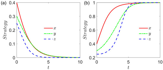
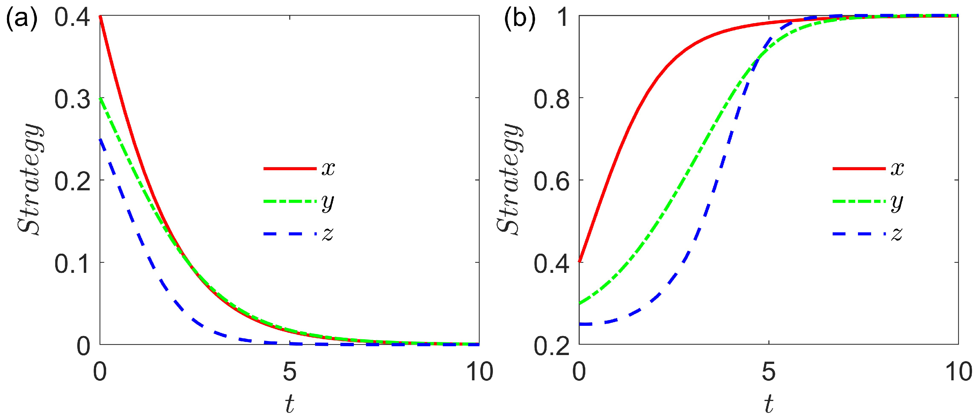
Figure 1 shows the time evolution of $x\left(t\right)$, $y\left(t\right)$, and $z\left(t\right)$ under two parameter settings without delays, namely ${\tau }_1=0$ and ${\tau }_2=0$. The initial state is set as $\left(x\right(0),y(0),z(0\left)\right)=(0.40,0.30,0.25)$, and the time interval is $t\in [0,10]$. Figure 1a corresponds to a low-incentive and low-return case. Under this parameter setting, the eigenvalues at $E_1=(0,0,0)$ are ${\lambda }_1=-0.70$, ${\lambda }_2=-0.70$, and ${\lambda }_3=-1.34$. Since all eigenvalues are negative, $E_1$ is locally asymptotically stable. Therefore, $x\left(t\right)$, $y\left(t\right)$, and $z\left(t\right)$ all decrease and finally approach zero. This means that when government incentives are weak, enterprise investment returns are low, and user adoption utility is insufficient, the system tends to fall into a traditional energy lock-in state. Figure 1b corresponds to a high-incentive and high-return case. Under this parameter setting, the eigenvalues at $E_8=(1,1,1)$ are ${\lambda }_1=-0.55$, ${\lambda }_2=-1.10$, and ${\lambda }_3=-2.26$. Since all eigenvalues are negative, $E_8$ is locally asymptotically stable. Thus, $x\left(t\right)$, $y\left(t\right)$, and $z\left(t\right)$ gradually increase and approach 1. This indicates that when government performance benefits, enterprise investment returns, and user adoption utility are sufficiently high, the system can evolve toward the coordinated state of active government incentives, enterprise new energy investment, and user new energy adoption. Overall, Figure 1 verifies the stability analysis of boundary equilibria. Under different parameter structures, the system may converge either to the low-level equilibrium $(0,0,0)$ or to the high-level equilibrium $(1,1,1)$.

Figure 1. Strategy evolution of the three agents in the delay-free case with the initial condition $\left(x\right(0),y(0),z(0\left)\right)=(0.40,0.30,0.25)$. (a) Under low policy incentives, low enterprise returns, and low user adoption utility, the numerical trajectories for the prescribed initial condition approach the locally asymptotically stable equilibrium $E_1=(0,0,0)$. The corresponding eigenvalues are $-0.70$, $-0.70$, and $-1.34$. Parameters are set as $M=0.20$, $C_g=1.00$, $S_g=0.20$, $S_u=0.10$, $L=0.10$, $R_e=0.30$, $C_e=0.60$, $R_t=0.40$, $P=0.20$, $B_u=0.20$, $C_u=0.50$, $T=0.20$, $\eta =0.10$, $\theta =0.10$, $D=0.10$, $\beta =0.40$, $k=6$, and $z_c=0.35$. (b) Under higher policy incentives, stronger enterprise returns, and higher user adoption utility, the numerical trajectories for the prescribed initial condition approach the locally asymptotically stable equilibrium $E_8=(1,1,1)$. The corresponding eigenvalues are $-0.55$, $-1.10$, and $-2.26$. Parameters are set as $M=1.20$, $C_g=0.30$, $S_g=0.20$, $S_u=0.15$, $L=0.40$, $R_e=0.80$, $C_e=0.60$, $R_t=0.40$, $P=0.25$, $B_u=0.70$, $C_u=0.50$, $T=0.30$, $\eta =0.25$, $\theta =0.30$, $D=0.20$, $\beta =0.40$, $k=6$, and $z_c=0.35$.

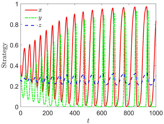
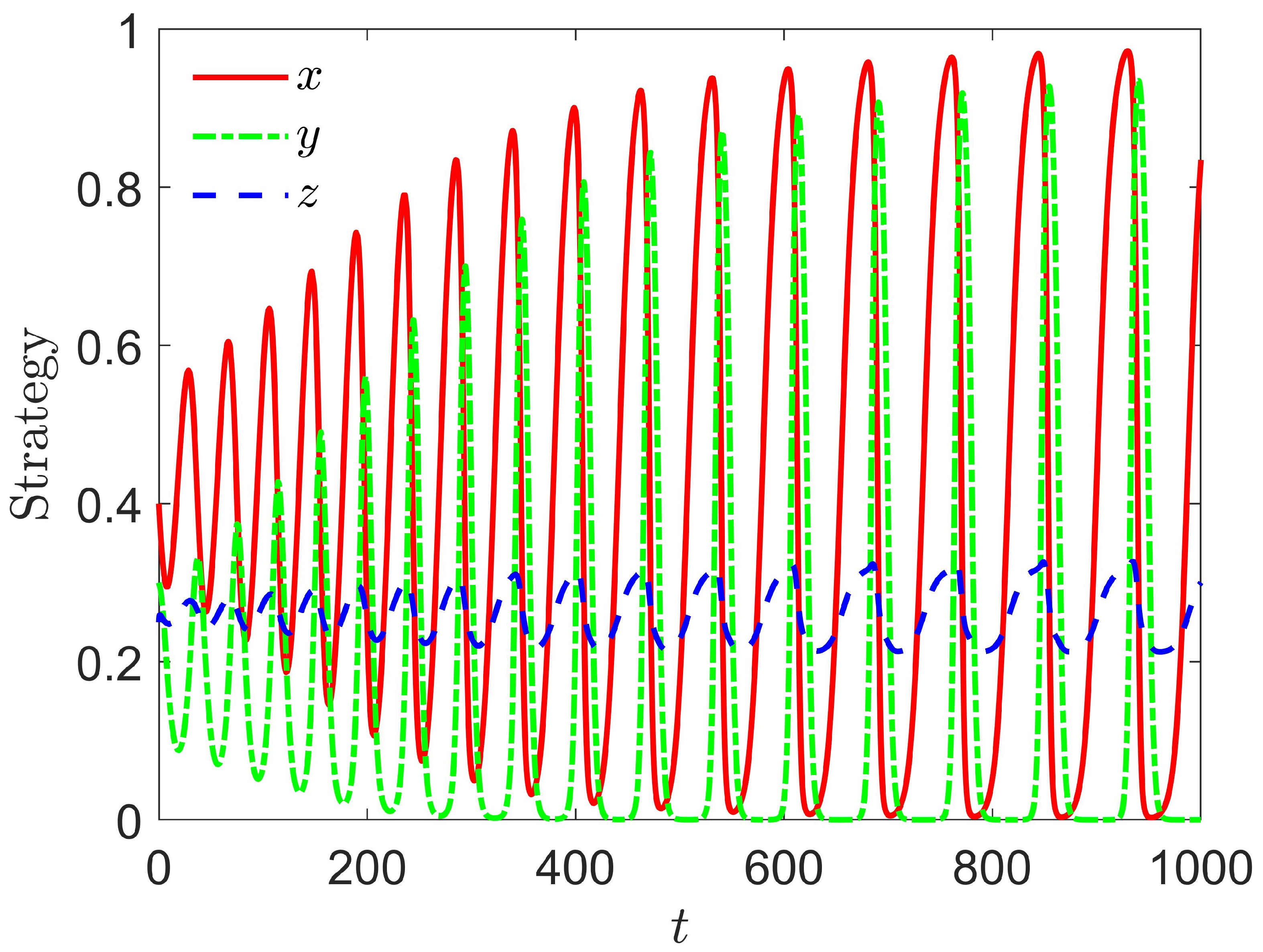
Figure 2 shows the dynamic evolution of $x\left(t\right)$, $y\left(t\right)$, and $z\left(t\right)$ when both delays are considered. Under the parameter setting ${\tau }_1=0.8$ and ${\tau }_2=0.5$, the three strategy variables do not converge to constant values but exhibit sustained oscillatory behavior. The government incentive proportion $x\left(t\right)$ and the enterprise investment proportion $y\left(t\right)$ fluctuate with relatively large amplitudes, whereas the user adoption proportion $z\left(t\right)$ varies within a comparatively smaller range. This numerical behavior is consistent with the theoretical finding that the local stability of the interior equilibrium depends jointly on ${\tau }_1$ and ${\tau }_2$. In particular, the characteristic equation indicates that a local Hopf bifurcation may occur at candidate points on the imaginary-root locus when the corresponding spectral and transversality conditions are satisfied. Therefore, Figure 2 should be interpreted as a representative numerical illustration of oscillatory dynamics under the selected double-delay parameter setting rather than as independent evidence for the occurrence of a Hopf bifurcation. In addition, the three curves exhibit clear phase differences. Changes in government incentives are followed by changes in enterprise investment and subsequently by changes in user adoption, reflecting the transmission process from policy to supply and then to demand. These phase differences are associated with the combined effects of the enterprise response delay ${\tau }_1$ and the user perception delay ${\tau }_2$. Economically, the coexistence of delayed enterprise responses to policy incentives and delayed user perceptions of supply improvements may lead to repeated adjustments among government incentives, enterprise investment, and user adoption. This suggests that improving the efficiency of policy transmission and market information dissemination may help mitigate undesirable oscillatory behavior in the new energy adoption process.

Figure 2. Strategy evolution processes of the three types of agents under double-delay conditions with the initial condition $\left(x\right(0),y(0),z(0\left)\right)=(0.40,0.30,0.25)$. The parameters are $M=0.766$, $C_g=0.615$, $S_g=0.723$, $S_u=0.495$, $L=0.135$, $R_e=0.402$, $C_e=0.177$, $R_t=0.821$, $P=0.560$, $B_u=0.234$, $C_u=0.749$, $T=0.799$, $\eta =0.134$, $\theta =0.297$, $D=0.2$, $\beta =-1.500$, $k=8$, and $z_c=0.301$, with delays ${\tau }_1=0.8$ and ${\tau }_2=0.5$.

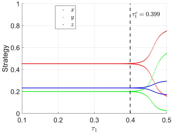
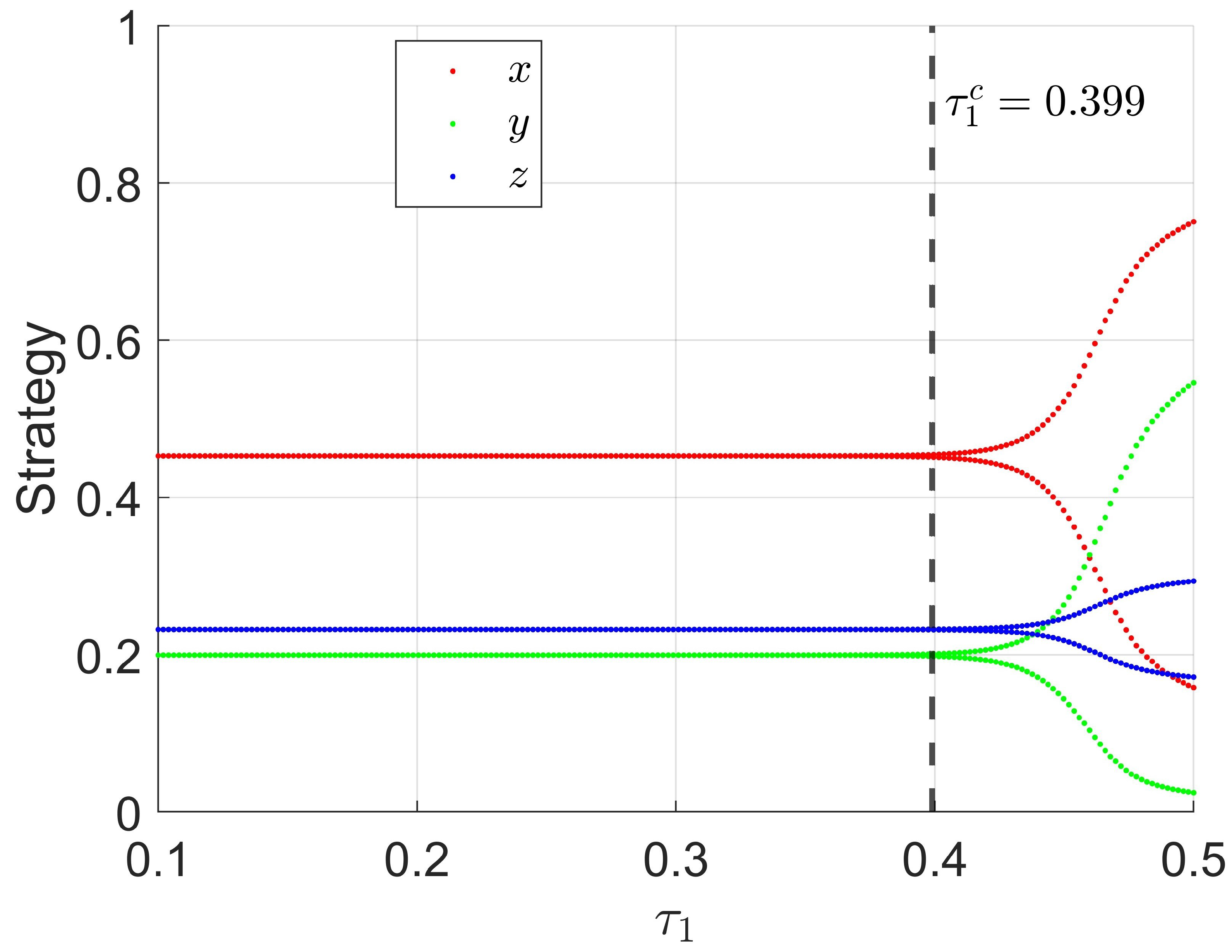
Figure 3 shows the effect of the policy response delay ${\tau }_1$ on the system when ${\tau }_2=0$. The red, green, and blue points represent the long-term maximum and minimum values of $x\left(t\right)$, $y\left(t\right)$, and $z\left(t\right)$, respectively. When the upper and lower branches coincide, the corresponding trajectories approach the interior equilibrium, whereas their separation indicates the emergence of oscillatory behavior. For ${\tau }_1<{\tau }_1^c=0.399$, the three variables converge to values close to the interior equilibrium $E^{*}=(0.45,0.20,0.23)$, indicating that sufficiently small policy response delays are compatible with local stability under the parameter setting considered. As ${\tau }_1$ passes through the critical value ${\tau }_1^c=0.399$, the upper and lower branches begin to separate, and oscillatory behavior is observed in the numerical range considered. Among the three variables, $x\left(t\right)$ exhibits the largest oscillation amplitude under this parameter setting, while the fluctuation of $y\left(t\right)$ is also pronounced and $z\left(t\right)$ varies more smoothly. The numerically observed transition near ${\tau }_1^c=0.399$ is consistent with the theoretical Hopf bifurcation condition derived in Section 3.2.1. It should be emphasized that this conclusion is local to the critical delay and does not imply that the equilibrium remains unstable for all larger values of ${\tau }_1$, since additional stability switches may occur. From a practical perspective, improving policy implementation efficiency and reducing excessive policy response delays may help mitigate delay-induced oscillatory behavior.

Figure 3. Bifurcation effect of the policy response delay ${\tau }_1$ when ${\tau }_2=0$. The parameters are $M=0.766$, $C_g=0.615$, $S_g=0.723$, $S_u=0.495$, $L=0.135$, $R_e=0.402$, $C_e=0.177$, $R_t=0.821$, $P=0.560$, $B_u=0.234$, $C_u=0.749$, $T=0.799$, $D=0.20$, $\eta =0.134$, $\theta =0.297$, $\beta =-0.78$, $k=8$, and $z_c=0.301$. The dashed line denotes the theoretical Hopf threshold ${\tau }_1^c=0.399$. Near the critical value ${\tau }_1^c$, the equilibrium may lose stability as ${\tau }_1$ crosses the threshold, and oscillatory behavior is observed in the numerical range considered.

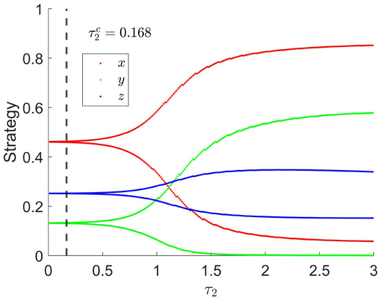
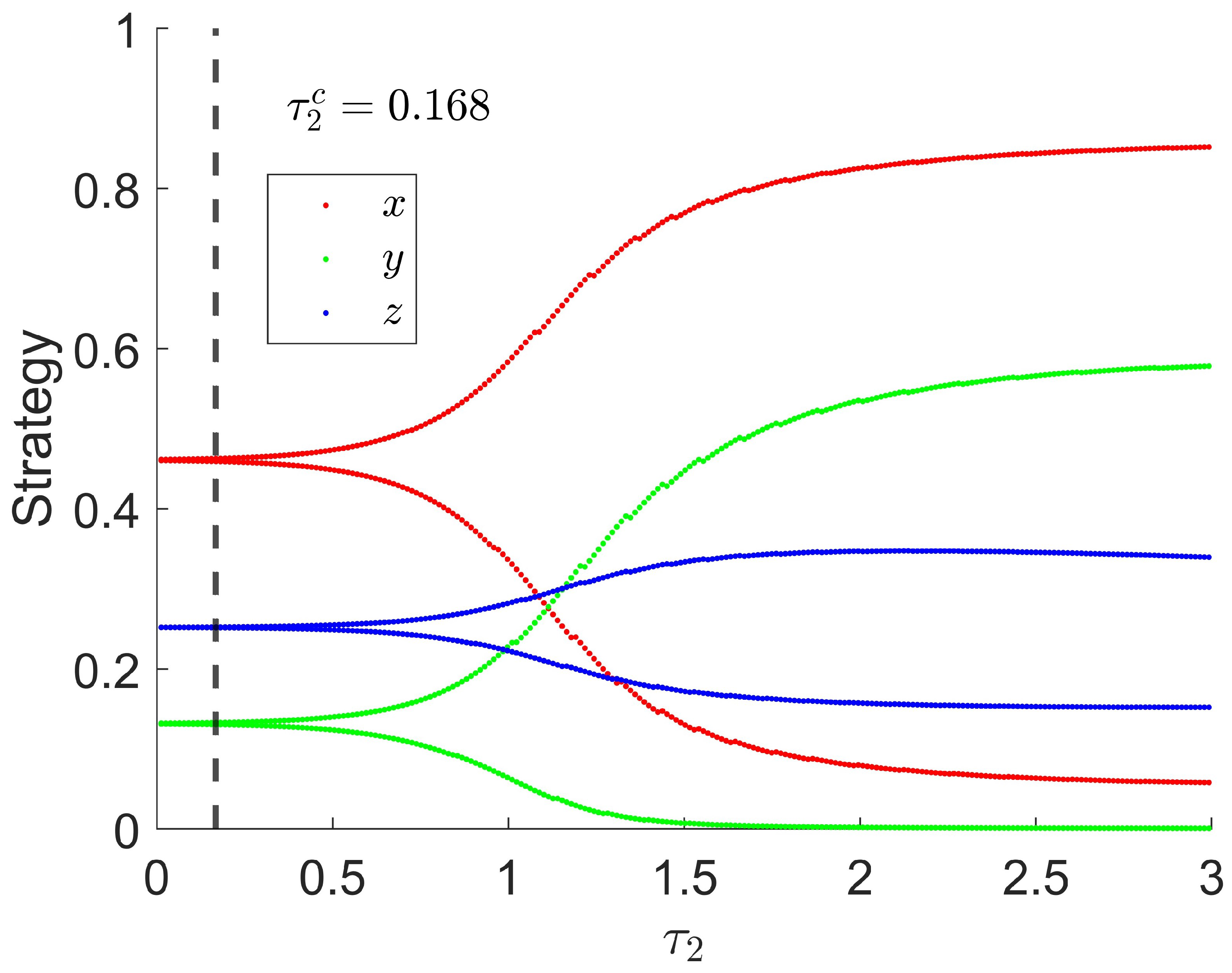
Figure 4 shows the effect of the user perception delay ${\tau }_2$ on the system when ${\tau }_1=0$. The red, green, and blue points represent the long-term maximum and minimum values of $x\left(t\right)$, $y\left(t\right)$, and $z\left(t\right)$, respectively. When the upper and lower branches coincide, the corresponding trajectories approach the interior equilibrium, whereas their separation indicates the emergence of oscillatory behavior. For ${\tau }_2<{\tau }_2^c=0.168$, the three variables converge to values close to the interior equilibrium $E^{*}=(0.4610,0.1317,0.2518)$, indicating that sufficiently small user perception delays are compatible with local stability under the parameter setting considered. As ${\tau }_2$ passes through the critical value ${\tau }_2^c=0.168$, the upper and lower branches begin to separate, and oscillatory behavior is observed in the numerical range considered. Within this range, the oscillation amplitudes increase as ${\tau }_2$ increases, suggesting that a larger user perception delay may intensify the mismatch between enterprise investment and user adoption. The numerically observed transition near ${\tau }_2^c=0.168$ is consistent with the theoretical Hopf bifurcation condition derived in Section 3.2.2. It should be emphasized that this conclusion is local to the critical delay and does not imply that the equilibrium remains unstable for all larger values of ${\tau }_2$, since additional stability switches may occur. From a practical perspective, reducing excessive user perception delays through improved information disclosure, user experience, infrastructure, and demonstration effects may help mitigate delay-induced oscillatory behavior.

Figure 4. Bifurcation effect of the user perception delay ${\tau }_2$ when ${\tau }_1=0$. The parameters are $M=0.766$, $C_g=0.615$, $S_g=0.723$, $S_u=0.687$, $L=0.135$, $R_e=0.402$, $C_e=0.177$, $R_t=0.821$, $P=0.497$, $B_u=0.234$, $C_u=0.749$, $T=0.473$, $\eta =0.099$, $\theta =1.603$, $D=0.20$, $\beta =-0.688$, $k=7.868$, and $z_c=0.301$. The dashed line denotes the theoretical Hopf threshold ${\tau }_2^c=0.168$. Near the critical value ${\tau }_2^c$, the equilibrium may lose stability as ${\tau }_2$ crosses the threshold, and oscillatory behavior is observed in the numerical range considered.

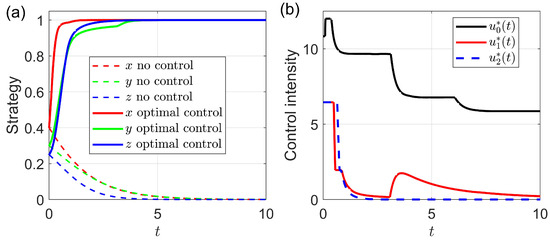
Figure 5 shows the system evolution and the corresponding optimal control paths. The initial state is set as $\left(x\right(0),y(0),z(0\left)\right)=(0.40,0.30,0.25)$, and the target state is $(x_d,y_d,z_d)=(1,1,1)$. The weight parameters are chosen as $Q_1=Q_2=Q_3=50$, $B_0=0.02$, $B_1=B_2=0.03$, and $D_1=D_2=D_3=1000$, while the upper bounds of the control variables are set as $u_0^{max}=12$, $u_1^{max}=10$, and $u_2^{max}=10$. The forward–backward sweep method is used for the numerical simulation. As shown in Figure 5a, without control, $x\left(t\right)$, $y\left(t\right)$, and $z\left(t\right)$ all decrease and eventually approach a low-level equilibrium near zero, indicating that the system lacks sufficient internal driving force and tends to fall into a traditional energy lock-in state. By contrast, under optimal control, the three variables increase rapidly and approach the target state $(1,1,1)$, showing that optimal control can effectively promote the transition from a low-adoption state to a high-adoption state. Figure 5b presents the optimal control paths. The institutional promotion intensity $u_0^{*}\left(t\right)$ rises quickly at the initial stage and then gradually decreases, while remaining at a relatively high level. The enterprise subsidy $u_1^{*}\left(t\right)$ first decreases and then increases in the middle stage, suggesting that enterprise support is still needed during the supply-side adjustment process. The user incentive $u_2^{*}\left(t\right)$ remains high in the early stage and then declines rapidly, indicating that demand-side incentives mainly play a start-up role. Overall, Figure 5 shows that the optimal control strategy can guide the system toward the target state through staged policy regulation, improve the convergence speed, and reduce the fiscal pressure caused by long-term high-intensity subsidies.

Figure 5. Dynamic evolution of the new energy adoption system under optimal control. (a) Under the parameters $M=0.20$, $C_g=1.00$, $S_g=0.20$, $S_u=0.10$, $L=0.10$, $R_e=0.30$, $C_e=0.60$, $R_t=0.40$, $P=0.20$, $B_u=0.20$, $C_u=0.50$, $T=0.20$, $\eta =0.10$, $\theta =0.10$, $D=0.10$, $\beta =0.40$, $k=6$, and $z_c=0.35$, the numerical trajectories starting from the initial state $(0.40,0.30,0.25)$ are shown for the uncontrolled and optimal-control cases; (b) the corresponding time paths of the optimal control strategies $u_0^{*}\left(t\right)$, $u_1^{*}\left(t\right)$, and $u_2^{*}\left(t\right)$. For the prescribed initial state, the uncontrolled trajectories approach a low-level equilibrium, whereas under optimal control, the trajectories are driven rapidly toward the target state $(1,1,1)$. The optimal control strategies exhibit clear stage-dependent and differentiated intervention patterns.

6. Conclusions

This paper develops a tripartite evolutionary game model to investigate the dynamic interactions among government incentives, enterprise investment, and user adoption in the new energy transition. Social feedback and two time delays are incorporated to characterize endogenous user interactions, delayed enterprise responses to policy incentives, and delayed user perceptions of supply improvements. The equilibrium structure and local stability properties of the system are analyzed, and the effects of the two delays on the stability of the interior equilibrium are further examined. The results show that the evolutionary dynamics depend jointly on payoff conditions, social feedback, and response delays. In the delay-free case, negative social feedback is a necessary condition for the local asymptotic stability of the interior equilibrium, although the remaining Routh–Hurwitz conditions must also be satisfied. For the single-delay cases, critical delay values are identified at which a pair of characteristic roots may cross the imaginary axis and a local Hopf bifurcation may occur under the corresponding spectral and transversality conditions. For the double-delay case, the interaction between the two delays gives rise to candidate imaginary-root loci in the $({\tau }_1,{\tau }_2)$ plane, along which the local stability of the interior equilibrium may change. The single-delay bifurcation diagrams and the double-delay time-domain simulations further illustrate the transition from equilibrium convergence to sustained oscillatory behavior near the corresponding critical conditions, as well as the phase differences among government, enterprise, and user strategies. An optimal control model is also formulated for the delay-free benchmark system. The numerical results show that appropriately designed time-dependent interventions can guide the system toward a high-adoption state while avoiding continuously high control intensity. The proposed optimal-control framework can, in principle, be extended to the delayed system. However, retaining the delays introduces advanced terms into the adjoint equations and leads to a more complicated forward–backward optimality system. Overall, the study highlights the important roles of delayed responses, social feedback, and policy intervention in shaping the local stability and evolutionary dynamics of new energy adoption. Several issues deserve further investigation. In particular, the direction of the Hopf bifurcation and the stability of the bifurcating periodic solutions can be further analyzed through center-manifold and normal-form techniques, including the calculation of the first Lyapunov coefficient. In addition, extending the optimal-control analysis to the full delayed system, together with the incorporation of heterogeneous networks and stochastic disturbances, represents an important direction for future research.

References

- Ossai, W.; Fagbola, T.M. Machine learning-based predictive modelling of renewable energy adoption in developing countries. Energy Rep. 2025, 14, 66–84. [Google Scholar] [CrossRef] [Scilit]
- Dhirasasna, N.; Sahin, O. A system dynamics model for renewable energy technology adoption of the hotel sector. Renew. Energy 2021, 163, 1994–2007. [Google Scholar] [CrossRef] [Scilit]
- Rahmani, A.; Daim, T.U.; Zamani, M.; Gungor, D.O. Renewable energy adoption: A meta-analysis of an extended technology acceptance model. Technol. Soc. 2026, 84, 103126. [Google Scholar] [CrossRef] [Scilit]
- Upton, G.B., Jr.; Snyder, B.F. Renewable energy potential and adoption of renewable portfolio standards. Util. Policy 2015, 36, 67–70. [Google Scholar] [CrossRef] [Scilit]
- Dogan, B.; Khalfaoui, R.; Bergougui, B.; Ghosh, S. Unveiling the impact of the digital economy on the interplay of energy transition, environmental transformation, and renewable energy adoption. Res. Int. Bus. Financ. 2025, 76, 102837. [Google Scholar] [CrossRef] [Scilit]
- Kamis, A.; Abraham, P.S. Predictive models of electric vehicle adoption in the United States: Charging ahead with renewable energy. Transp. Res. Interdiscip. Perspect. 2024, 24, 101041. [Google Scholar] [CrossRef] [Scilit]
- Xu, H.J.; Huang, C.W.; Xia, C.Y. The evolution of fairness induced by marginal loss in ultimatum games within the networked population. Appl. Math. Model. 2026, 155, 116753. [Google Scholar] [CrossRef] [Scilit]
- Luo, C.Y.; Zhang, Y.J.; Feng, M.Y.; Szolnoki, A. Evolutionary cooperation with game transitions via Markov decision chain in networked population. Appl. Math. Model. 2026, 154, 116710. [Google Scholar] [CrossRef] [Scilit]
- Xiao, L.; Liu, J.Y.; Ge, J.W. Dynamic game in agriculture and industry cross-sectoral water pollution governance in developing countries. Agric. Water Manag. 2021, 243, 106417. [Google Scholar] [CrossRef] [Scilit]
- Xie, F.; Guo, Z.W.; Li, T.; Feng, Q.C.; Zhao, C.J. Dynamic task planning for multi-arm harvesting robots under multiple constraints using deep reinforcement learning. Horticulturae 2025, 11, 88. [Google Scholar] [CrossRef] [Scilit]
- Ding, M.Z.; Bai, Y.L.; Wang, C.Y. Governance of corporate misconduct through employee whistleblowing: A tripartite evolutionary game analysis. BMC Psychol. 2026, 14, 722. [Google Scholar] [CrossRef] [Scilit]
- Li, S.X.; Wang, X. A tripartite evolutionary game analysis of the low-carbon transition for nearly zero-energy office buildings. Buildings 2026, 16, 1122. [Google Scholar] [CrossRef] [Scilit]
- Mishra, R.; Naik, B.K.R.; Raut, R.D.; Kumar, M. Internet of Things (IoT) adoption challenges in renewable energy: A case study from a developing economy. J. Clean. Prod. 2022, 371, 133595. [Google Scholar] [CrossRef] [Scilit]
- Mustafa, S.; Zhang, W.; Sohail, M.T.; Rana, S.; Long, Y. A moderated mediation model to predict the adoption intention of renewable wind energy in developing countries. PLoS ONE 2023, 18, e0281963. [Google Scholar] [CrossRef] [Scilit]
- Li, X.Y.; Li, C.J.; Chen, G.; Dong, Z.Y. A risk-averse energy sharing market game for renewable energy microgrid aggregators. IEEE Trans. Power Syst. 2022, 37, 3528–3539. [Google Scholar] [CrossRef] [Scilit]
- Zhang, Y.J.; Gu, C.H.; Yan, X.H.; Li, F.R. Cournot oligopoly game-based local energy trading considering renewable energy uncertainty costs. Renew. Energy 2020, 159, 1117–1127. [Google Scholar] [CrossRef] [Scilit]
- Xu, H.T.; Hui, H.W.; Zhou, C.C.; Zeng, G.P.; Han, Z. Cooperative energy trading for HetNets with renewable energy: A dynamic energy trading game. IEEE Internet Things J. 2024, 11, 11606–11618. [Google Scholar] [CrossRef] [Scilit]
- Abbas, M.; Zhang, Y.M.; Koura, Y.H.; Su, Y.Y.; Iqbal, W. The dynamics of renewable energy diffusion considering adoption delay. Sustain. Prod. Consum. 2022, 30, 387–395. [Google Scholar] [CrossRef] [Scilit]
- Yu, Y.; Xiao, X.P.; Gao, M.Y.; Rao, C.J. Dynamic time-delay discrete grey model based on GOWA operator for renewable energy generation cost prediction. Renew. Energy 2025, 242, 122408. [Google Scholar] [CrossRef] [Scilit]
- Ouyang, N.N.; Guo, L.N.; Hong, C.; Zhang, X.Y.; Liu, Y.Y.; Guo, Y.T.; Wang, Y.C.; Ma, H.L. Effects of delayed tuber cutting after catalytic infrared heat treatment on browning of fresh-cut potatoes and its potential mechanisms. Food Chem. 2025, 480, 143834. [Google Scholar] [CrossRef] [Scilit]
- Wang, J.Z.; Gao, Z.H.; Zhang, Y.; Zhou, J.; Wu, J.Z.; Li, P.P. Real-time detection and location of potted flowers based on a ZED camera and a YOLO V4-Tiny deep learning algorithm. Horticulturae 2022, 8, 21. [Google Scholar] [CrossRef] [Scilit]
- Lan, T.K.; Sun, H.D.; Wang, Q.; Zhao, B. Synthesis load model with renewable energy sources for transient stability studies. IEEE Trans. Power Syst. 2024, 39, 1647–1663. [Google Scholar] [CrossRef] [Scilit]
- Dileep, G.; Singh, S.N.; Singh, G.K. Modelling, design and stability analysis of an improved SEPIC converter for renewable energy systems. Int. J. Electron. 2017, 104, 1527–1545. [Google Scholar] [CrossRef] [Scilit]
- Wang, Z.C.; He, W.; Sun, J.; Wang, G. Time-delay effects on the dynamical behavior of switched nonlinear time-delay systems. Sci. China Inf. Sci. 2025, 68, 179201. [Google Scholar] [CrossRef] [Scilit]
- Huang, Z.Q.; Fan, C.C.; Mitra, S. Bounded invariant verification for time-delayed nonlinear networked dynamical systems. Nonlinear Anal. Hybrid Syst. 2017, 23, 211–229. [Google Scholar] [CrossRef] [Scilit]
- Kalmár-Nagy, T.; Horváth, D.A. Numerical Hopf normal form for delay-differential equations. Nonlinear Dyn. 2025, 113, 16383–16399. [Google Scholar] [CrossRef] [Scilit]
- Pei, L.J.; Wang, K.W. Hopf-Hopf bifurcation and chaos in delay-coupled reservoir computing system with two delays. Int. J. Non-Linear Mech. 2023, 155, 104452. [Google Scholar] [CrossRef] [Scilit]
- Alemu, S.M.; Dawed, M.Y.; Mamo, T.T. Eco-epidemiological mathematical model analysis with time delays and Hopf bifurcation. Nat. Resour. Model. 2026, 39, e70033. [Google Scholar] [CrossRef] [Scilit]
- Chen, Y.; Ma, Z.P. Stability and Hopf bifurcation of Nicholson’s blowflies model with delayed linear harvesting. Int. J. Bifurc. Chaos 2026, 36, 2650095. [Google Scholar] [CrossRef] [Scilit]
- Sun, F. Organizational responsiveness in a three-dimensional discrete model of AI, ESG disclosure, and green supply chain collaboration. J. Nonlinear Dyn. Appl. 2026, 2, 159–176. [Google Scholar] [CrossRef] [Scilit]
- Hossain, M.; Hosen, M.; Lin, W.L.; Pek, C.K.; Chong, S.C. Dynamic interactions between circular economy, technological innovation, and renewable energy for sustainable development. Sustain. Dev. 2026. [Google Scholar] [CrossRef] [Scilit]
- Li, L.H.; Zhuang, X.W.; Dong, B.H.; Gan, C.S.P. A systemic analysis of green finance, renewable energy investment, and regional economic growth in China: The role of social technical interactions and behavioral factors. Systems 2026, 14, 384. [Google Scholar] [CrossRef] [Scilit]
- Yan, J.K.; Wang, Z.W.; Wang, L.; Liu, Z.C.; Yu, Y.H.; Jin, M.; Li, L.Q.; Li, L. Insights into the complex coacervation behavior and interaction mechanism of nisin and rhamnolipid. J. Sci. Food Agric. 2025, 105, 4758–4770. [Google Scholar] [CrossRef] [Scilit]
- Appah, S.; Wang, P.; Ou, M.X.; Gong, C.; Jia, W.D. Review of electrostatic system parameters, charged droplets characteristics and substrate impact behavior from pesticides spraying. Int. J. Agric. Biol. Eng. 2019, 12, 1–9. [Google Scholar] [CrossRef] [Scilit]
- Waqas, M.; Yahya, F.; Ahmed, A.; Rasool, Y.; Li, H. Unlocking employee’s green behavior in fertilizer industry: The role of green HRM practices and psychological ownership. Int. Food Agribus. Manag. Rev. 2021, 24, 827–843. [Google Scholar] [CrossRef] [Scilit]
- Zhang, Y.; Yang, F.; Mao, Y.Y.; Jiao, L.D.; Huo, X.S.; Shuai, C.Y. Green growth in the digital age: The causal interactions between digital finance, green technology innovation, and ecological welfare performance. Technol. Soc. 2026, 87, 103343. [Google Scholar] [CrossRef] [Scilit]
- Wang, L.P.; Chen, L.J.; Wang, Z.J.; Li, C. Exploring strategies for promoting green technology innovation in enterprises from the perspective of inter-enterprise interaction and enterprise behavioral preferences. Renew. Energy 2025, 250, 123287. [Google Scholar] [CrossRef] [Scilit]
- Zhou, T.F.; Hu, C. Commercialization path of data-driven green catalytic technology: The application of machine learning in technology lifecycle management. Environ. Res. 2026, 296, 123925. [Google Scholar] [CrossRef] [Scilit]
- Zhang, X.F.; Yin, S.; Li, M. Research on the mechanism and path of the coupling of digital technology and environmental regulation to promote urban green efficiency. Sustain. Cities Soc. 2024, 116, 105906. [Google Scholar] [CrossRef] [Scilit]
- Liu, L.; Zhang, L.; Xu, W. Research on the enhancement path of green technology innovation efficiency under the group perspective. PLoS ONE 2024, 19, e0306936. [Google Scholar] [CrossRef] [Scilit]
Disclaimer/Publisher’s Note: The statements, opinions and data contained in all publications are solely those of the individual author(s) and contributor(s) and not of MDPI and/or the editor(s). MDPI and/or the editor(s) disclaim responsibility for any injury to people or property resulting from any ideas, methods, instructions or products referred to in the content. |
© 2026 by the authors. Licensee MDPI, Basel, Switzerland. This article is an open access article distributed under the terms and conditions of the Creative Commons Attribution (CC BY) license.