Privacy-Preserving Distributed Online Dispatch of Low-Carbon Microgrids with TCN–BiLSTM Probabilistic Photovoltaic Forecasts

Abstract

Low-carbon microgrids are complex energy systems in which photovoltaic (PV) uncertainty, time-varying operating costs, distributed coordination, and information privacy must be addressed simultaneously. This paper couples TCN–BiLSTM probabilistic PV forecasting with privacy-preserving distributed online economic dispatch. Quantile forecasts are converted into a risk-aware net demand by combining the median PV forecast with a lower-side uncertainty reserve. The resulting dispatch problem also includes a step-type carbon-trading cost. To solve the problem when cost gradients are unavailable, we propose a probabilistic PV forecasting-driven differentially private distributed online one-point bandit optimization algorithm (PPF-DP-DOBO). Each generator uses one function-value query per iteration and perturbs its communicated state with Laplace noise. The analysis establishes a per-release differential privacy guarantee, its sequential composition over the dispatch horizon, and an individual dynamic regret bound that explicitly depends on PV forecasting uncertainty. Under bounded weighted path variation and cumulative forecasting uncertainty, the regret is sublinear with order $\mathcal{O}\left(T^{3/4}\right)$. Simulations on a modified IEEE 162-bus system show that the method tracks the risk-aware net demand, preserves the expected privacy–performance trade-off, and yields lower average regret and carbon cost in the evaluated probabilistic-PV setting than in the no-PV case.

1. Introduction

Low-carbon microgrids combine renewable generation, conventional distributed generators (DGs), communication networks, and market mechanisms in a tightly coupled complex system. Their operating state is nonlinear and time-varying because electricity demand, renewable generation, and generation costs evolve on different time scales. Photovoltaic (PV) generation further increases this variability, but it also reduces the demand supplied by carbon-emitting units. Effective microgrid operation therefore requires a dispatch method that can use renewable forecasts, coordinate distributed units, and adapt online without exposing sensitive operating information [1,2,3]. The work in Ref. [4] further indicates that distributed economic dispatch research is progressively extending from basic consensus-based allocation toward renewable-rich operation, practical engineering constraints, and privacy-preserving coordination.

A deterministic PV point forecast does not describe the asymmetric risk of PV underproduction. Probabilistic forecasting addresses this limitation by estimating quantiles or prediction intervals rather than a single trajectory [5,6]. In this work, a temporal convolutional network and bidirectional long short-term memory network (TCN–BiLSTM) model short- and long-range dependencies in PV and meteorological time series. Its median forecast represents the expected PV contribution, whereas a lower quantile defines the reserve required to hedge against underproduction. This construction provides a direct interface between machine-learning-based uncertainty estimation and risk-aware dispatch. The work in Ref.  [7] also employs a robust multi-objective optimization method to consider the uncertainties of renewable energy generation and load in uncertainty-aware microgrid research.

The dispatch problem is also challenging when generator costs are time-varying or available only through function-value queries. Distributed gradient methods have been widely studied for economic dispatch [8,9,10], but they require explicit gradients or sufficiently accurate gradient evaluations. Gradient-free online optimization instead constructs an update direction from queried function values [11,12,13]. Two-point estimators offer favorable accuracy but require two evaluations per update [14,15]. One-point bandit feedback reduces this requirement to one query and is therefore attractive for online energy systems with limited computational or communication resources [16,17,18,19].

Distributed communication introduces a second source of risk. Exchanged generator states may reveal operating conditions or cost-related information to an observer. Differential privacy provides a mathematically explicit way to bound the influence of an adjacent input on a released state [20]. Existing privacy-preserving dispatch methods protect state exchange under several network and optimization settings [21,22,23,24]. For microgrid applications, the work in Ref. [25] proposes a distributed differentially private consensus controller that combines nondecaying noise with a time-varying control gain to protect exchanged information while maintaining frequency regulation and active-power sharing. The method proposed in Ref. [26] integrates attenuated differential privacy and fully homomorphic encryption into distributed alternating direction method of multipliers to protect generator information during distributed microgrid energy management. However, privacy noise degrades coordination accuracy, and its cumulative effect must be distinguished from the uncertainty already introduced by renewable forecasting.

Dynamic regret is the appropriate performance measure for this setting because the optimal dispatch changes with load, PV output, and operating costs [27,28,29,30,31]. Existing online bandit and privacy-preserving dispatch studies do not jointly expose how forecast uncertainty, one-point feedback, privacy perturbations, and a time-varying comparator affect the regret bound. Moreover, treating probabilistic forecasting and online dispatch as unrelated modules obscures how prediction intervals alter the mathematical dispatch target.

Accordingly, a research gap remains between uncertainty-aware microgrid scheduling, privacy-preserving distributed optimization, and cyber-resilient reconfiguration: existing studies generally emphasize one or two of these aspects, whereas their combined influence on a distributed online bandit regret bound has received limited attention.

This paper addresses this gap through PPF-DP-DOBO, a probabilistic PV forecasting-driven differentially private distributed online one-point bandit optimization method. The TCN–BiLSTM forecaster first produces PV quantiles. The median and lower quantile are then mapped to a risk-aware net demand, which becomes the time-varying dispatch target. The dispatch stage uses one function-value query to estimate a search direction and adds Laplace noise to communicated generator states. A step-type carbon-trading cost represents the increasing economic penalty of high-emission operation. The comparison with recent works is listed in Table 1.

Table 1. Qualitative comparison of representative distributed economic dispatch and online optimization approaches.

Method Class	Cost Information	PV Uncertainty	State Privacy	Main Scope
Distributed gradient economic dispatch [8,9,10]	Exact or evaluated gradients	Not jointly modeled	Not the primary objective	Economic dispatch with distributed coordination
Two-point gradient-free methods [14,15]	Two function queries per update	Not jointly modeled	Not the primary objective	Zeroth-order online optimization
Privacy-preserving economic dispatch [21,22,23,24]	Method dependent	Not jointly modeled	Explicitly protected	Protected coordination of generator states
Proposed PPF-DP-DOBO	One function query per update	TCN–BiLSTM quantile forecasts	Differential privacy	Risk-aware, low-carbon, distributed online dispatch

The main contributions are as follows.

(1)

A forecast-to-dispatch coupling is developed for low-carbon microgrids. TCN–BiLSTM quantile forecasts are converted into a median PV contribution and a lower-side uncertainty reserve. These quantities define a risk-aware net demand and connect data-driven temporal uncertainty with the economic dispatch model.

(2)

A privacy-preserving distributed online dispatch method is formulated for unknown time-varying cost functions. PPF-DP-DOBO uses one function-value query per generator and iteration, while Laplace perturbations protect communicated power states. The privacy analysis distinguishes the per-release privacy budget from its sequential composition over the dispatch horizon.

(3)

A conditional dynamic-regret guarantee is derived for the coupled forecasting and dispatch system. The bound contains both the weighted path variation of the dynamic optimum and the cumulative PV forecasting uncertainty. Simulations on a modified IEEE 162-bus system evaluate forecasting behavior, supply–demand tracking, carbon cost, dynamic regret, baseline performance, and the privacy–performance trade-off.

The remainder of this paper is organized as follows. Section 2 introduces the communication and privacy preliminaries, the TCN–BiLSTM probabilistic forecaster, and the low-carbon dispatch problem. Section 3 presents PPF-DP-DOBO and its theoretical guarantees. Section 4 reports the numerical experiments, Section 5 discusses their implications and limitations, and Section 6 concludes the paper.

Notation 1.

The set of real numbers is denoted by $\mathbb{R}$, and ${\mathbb{R}}^d$ is the d-dimensional Euclidean space. The feasible decision set is Ω, and ${\Pi }_{\Omega }\left[x\right]=\arg {\min }_{\widehat{x}\in \Omega }{\parallel \widehat{x}-x\parallel }^2$ denotes the Euclidean projection. The unit sphere in ${\mathbb{R}}^d$ is ${\mathbb{S}}^d$. The TCN–BiLSTM quantile forecaster is ${\mathcal{F}}_{\theta }$, where θ contains its trainable parameters. The input window is $X_t$, the q-quantile PV forecast is ${\widehat{p}}_{pv}^{\left(q\right),t}$, the lower-side reserve is $R_{pv}^t$, the risk-aware net demand is $P_{\mathrm{net}}^t$, and cumulative PV forecasting uncertainty is ${\mathcal{U}}_{pv,T}$.

2. Preliminaries and Problem Formulation

2.1. Graph Theory

A directed graph $\mathcal{G}:=(\mathcal{V},\mathcal{E})$ is employed to model information sharing among N agents. The graph $\mathcal{G}$ comprises a vertex set $\mathcal{V}=\{1,2,\dots ,N\}$ and edge set $\mathcal{E}\subseteq \mathcal{V}\times \mathcal{V}$. The connectivity of $\mathcal{G}$ is ensured by the existence of a path that links any pair of agents. We utilize $N_i^{in}=\{\left.j\in \mathcal{V}\right|(j,i)\in \mathcal{E}\}$ to represent the number of edges that point to agent i (in-neighbors), and $N_i^{out}=\{\left.j\in \mathcal{V}\right|(i,j)\in \mathcal{E}\}$ to represent the number of edges departing from agent i (out-neighbors). Let $A=\left[a_{ij}\right]\in {\mathbb{R}}^{N\times N}$ be the weighted adjacency matrix of $\mathcal{G}$, where $a_{ij}$ represents the weight assigned to the edge $(i,j)$.

2.2. Differential Privacy

Differential privacy is a pivotal and indispensable concept and technology in the field of privacy protection, serving as a vital tool to address the inherent risks posed by the potential disclosure of sensitive personal information during data analysis and sharing. Traditional approaches to privacy protection, such as de-identification or encryption, commonly prove inadequate in effectively mitigating the re-identification of personal data. In contrast, differential privacy provides a robust and rigorously defined framework that ensures the preservation of individuals’ privacy by incorporating controlled perturbation techniques during the data processing phase. Therefore, this paper will employ differential privacy techniques to effectively protect the privacy of generator power information. Next, we first give the following definitions.

Definition 1.

Given two different datasets Θ and ${\Theta }^{\prime }$, if Θ can be obtained by adding, deleting, or modifying a single element from ${\Theta }^{\prime }$, then Θ and ${\Theta }^{\prime }$ are considered adjacent.

Definition 2.

For any adjacent inputs Θ and ${\Theta }^{\prime }$ and any measurable output set ψ, a randomized mechanism $\mathrm{M}$ is ε-differentially private if

$$\begin{array}{c}\hfill \mathbb{P}[\mathrm{M}(\Theta )\in \psi ]\le e^{\epsilon }\mathbb{P}[\mathrm{M}\left({\Theta }^{\prime }\right)\in \psi ],\end{array}$$

(1)

where the probability is taken over the internal randomness of $\mathrm{M}$.

Definition 3.

Let $q_t(\Theta )$ denote the deterministic vector-valued state query to be released at time t. Its global ${\mathsf{\ell }}_1$-sensitivity over adjacent inputs is defined as

$$\begin{array}{cc}\hfill {\Delta }_t& =\underset{\Theta \sim {\Theta }^{\prime }}{\sup }{∥q_t(\Theta )-q_t\left({\Theta }^{\prime }\right)∥}_1,\hfill \end{array}$$

(2)

where $\Theta \sim {\Theta }^{\prime }$ denotes that Θ and ${\Theta }^{\prime }$ are adjacent according to Definition 1.

In the present dispatch setting, two inputs are adjacent if they differ only in one private local generation or cost record of one generator at one time, while the public load profile, PV forecasts, communication topology, and all other generators’ records remain unchanged. The deterministic query is the stacked generator-state vector $q_t(\Theta )={\mathbf{p}}_t(\Theta )$, and the released mechanism is ${\mathrm{M}}_t(\Theta )=q_t(\Theta )+{\eta }_t$. Therefore, one release refers to the joint communicated state vector at one dispatch time rather than to each individual scalar component.

The parameter ${\epsilon }_t>0$ is the dimensionless privacy-loss budget assigned to the release at time t. Inequality (1) shows that changing one private record can change the probability of any released event by at most the multiplicative factor $e^{{\epsilon }_t}$. A smaller ${\epsilon }_t$ makes the output distributions under adjacent inputs closer and therefore provides stronger privacy, but it increases the Laplace scale ${\sigma }_t={\Delta }_t/{\epsilon }_t$ and may reduce dispatch accuracy. Conversely, a larger ${\epsilon }_t$ introduces less noise but provides weaker privacy protection.

Because the mechanism releases one state vector at every dispatch time, ${\epsilon }_t$ is a per-release budget rather than the privacy guarantee for the entire dispatch horizon. Under sequential composition, the pure-differential-privacy budget accumulated from time 0 to time T is

$$\begin{array}{cc}\hfill {\epsilon }_{\mathrm{tot}}\left(T\right)& ={\displaystyle \sum _{t=0}^T}{\epsilon }_t.\hfill \end{array}$$

(3)

Thus, using a constant per-release budget ${\epsilon }_t=\epsilon$ results in ${\epsilon }_{\mathrm{tot}}\left(T\right)=(T+1)\epsilon$. For a prescribed finite-horizon budget $\overline{\epsilon }$, the release budgets should instead be selected such that ${\sum }_{t=0}^T{\epsilon }_t\le \overline{\epsilon }$; for example, the uniform allocation ${\epsilon }_t=\overline{\epsilon }/(T+1)$ is privacy-feasible for a fixed horizon. The resulting guarantee protects the released generator states against inference under the stated adjacency relation, but it does not by itself prevent active message falsification, denial-of-service attacks, or physical manipulation of the microgrid.

Remark 1.

The game-theoretic framework in Ref. [32] uses a Stackelberg game to mitigate false-data-injection attacks and dynamically reconfigure interconnected microgrids for secure and cost-efficient operation. In contrast, PPF-DP-DOBO employs sensitivity-calibrated Laplace noise to limit information inference from communicated generator states. Thus, the former addresses active cyberattacks and network resilience, whereas the latter protects information privacy during distributed online dispatch. Their integration is left for future research.

2.3. TCN-BiLSTM-Based Probabilistic Photovoltaic Power Forecasting Model

Accurate photovoltaic (PV) power forecasting is essential for reliable economic dispatch under renewable energy uncertainty. However, PV generation exhibits strong temporal fluctuations and nonlinear characteristics due to the combined influence of historical power outputs and meteorological conditions. To address these challenges, a hybrid temporal convolutional network and bidirectional long short-term memory network (TCN-BiLSTM) is developed in this paper for probabilistic PV power forecasting.

The proposed forecasting model integrates the advantages of temporal convolutional networks (TCNs) and bidirectional long short-term memory networks (BiLSTMs). The TCN module is responsible for extracting multi-scale temporal patterns from historical PV generation sequences through causal dilated convolutions, while the BiLSTM module captures long-range temporal dependencies by considering information from both forward and backward directions.

Given the historical PV power and meteorological feature sequence, the input vector at time t is defined as follows:

$$X_t=[x_{t-N+1},x_{t-N+2},\cdots ,x_t]$$

(4)

where N represents the length of the historical observation window. Specifically, the feature vector at time t is defined as ${\mathbf{x}}_t={[p_{pv}^t,G_t^{\mathrm{GHI}},G_t^{\mathrm{GTI}},G_t^{\mathrm{DHI}},T_t,H_t]}^{\mathrm{T}}$, where $p_{pv}^t$ denotes the historical PV power output, $G_t^{\mathrm{GHI}}$, $G_t^{\mathrm{GTI}}$, and $G_t^{\mathrm{DHI}}$ denote the global horizontal irradiance, global tilted irradiance, and diffuse horizontal irradiance, respectively, $T_t$ denotes the ambient temperature, and $H_t$ denotes the relative humidity. Therefore, $X_t$ contains both the recent PV-generation trajectory and the meteorological conditions associated with solar-resource availability and environmental variations.

The TCN module consists of multiple residual temporal convolution blocks. Different from conventional convolutional neural networks, TCN adopts causal convolution to preserve the temporal order of historical information and utilizes dilation factors to enlarge the receptive field.

The feature extraction process of the TCN module can be formulated as follows:

$$Z_t^{\left(l\right)}=\sigma (W_l{\ast }_d{Z}_t^{(l-1)}+b_l)$$

(5)

where $Z_t^{\left(l\right)}$ denotes the output feature representation of the l-th TCN layer, $W_l$ and $b_l$ represent convolution parameters, ${\ast }_d$ denotes dilated causal convolution operation with dilation factor d, and $\sigma (·)$ is the nonlinear activation function.

Through the dilation mechanism, the TCN module can effectively extract both short-term fluctuation characteristics and long-term variation trends of PV generation without significantly increasing computational complexity.

After temporal feature extraction, the obtained feature sequence is further processed by the BiLSTM network. The hidden representation generated by the BiLSTM module is expressed as follows:

$$h_t=BiLSTM\left(Z_t^{\left(L\right)}\right)$$

(6)

where $h_t$ represents the temporal feature representation learned by the BiLSTM network.

The BiLSTM structure contains two independent LSTM networks, including forward and backward propagation paths. Therefore, the model can simultaneously utilize historical and future information within the input window, improving the ability to capture nonlinear temporal dependencies caused by weather variations.

The final probabilistic PV power prediction output is obtained through a fully connected layer:

$${\widehat{\mathbf{p}}}_{pv}^t={\mathcal{F}}_{\theta }\left(X_t\right)=W_o{h}_t+b_o$$

(7)

where ${\mathcal{F}}_{\theta }$ denotes the proposed TCN-BiLSTM forecasting network parameterized by $\theta$, and ${\widehat{\mathbf{p}}}_{pv}^t$ represents the predicted PV power under different quantile levels.

To characterize forecasting uncertainty, multiple quantile outputs are generated:

$${\widehat{\mathbf{p}}}_{pv}^t=[{\widehat{p}}_{q_1}^t,{\widehat{p}}_{q_2}^t,\cdots ,{\widehat{p}}_{q_m}^t]$$

(8)

where $q_m$ denotes the corresponding quantile level.

The forecasting model is trained by minimizing the quantile regression loss function:

$${\mathcal{L}}_{pv}\left(\theta \right)={\displaystyle \frac{1}{mT}}{\displaystyle \sum _{t=1}^T}{\displaystyle \sum _{r=1}^m}{\rho }_{q_r}\left({\left[{\mathcal{F}}_{\theta }\left(X_t\right)\right]}_r,p_{pv}^t\right)$$

(9)

where the pinball loss for quantile $q\in (0,1)$ is

$${\rho }_q(\widehat{p},p):=\left(q-{\mathbf{1}}_{\{p<\widehat{p}\}}\right)(p-\widehat{p}),$$

(10)

and ${\mathbf{1}}_{\{·\}}$ is the indicator function. This objective penalizes under- and over-prediction asymmetrically and yields the quantiles used by the dispatch stage.

To improve the reproducibility of the forecasting model, its main hyperparameters are summarized in Table 2. The input window contains 24 consecutive samples. The TCN component comprises three temporal convolution layers with a kernel size of 3 and dilation factors of 1, 2, and 4. The extracted temporal features are processed by a two-layer BiLSTM network with 64 hidden units. The model is trained for 100 epochs using the Adam optimizer with a learning rate of 0.001 and a batch size of 32.

Table 2. Hyperparameters of the proposed TCN–BiLSTM forecasting model.

Parameter	Value
Input window size	24
Number of TCN layers	3
Kernel size	3
Dilation factors	1, 2, 4
BiLSTM layers	2
Hidden units	64
Optimizer	Adam
Learning rate	0.001
Batch size	32
Training epochs	100

Compared with conventional CNN-based forecasting approaches, the proposed TCN-BiLSTM model provides two advantages. First, the TCN structure captures multi-scale temporal characteristics through dilated causal convolutions, which is suitable for PV sequences with periodic fluctuations and sudden changes. Second, the BiLSTM structure enhances the modeling capability of long-term dependencies by utilizing bidirectional temporal information.

The resulting median and lower-quantile forecasts provide, respectively, the expected operating trajectory and the lower-tail uncertainty information required by the subsequent dispatch formulation.

2.4. Problem Formulation

The EDP within a microgrid entails considering every conventional generator as a node and synchronizing all nodes to minimize production costs while adhering to supply–demand equilibrium and generation constraints. Consequently, the EDP within a microgrid fundamentally represents a constrained optimization challenge. Additionally, in the context of low-carbon electricity, energy conservation and emission reduction have become important objectives for microgrid systems. To simultaneously consider the economic and environmental aspects of a microgrid, this paper integrates a carbon-trading mechanism into its economic dispatch model.

Different from deterministic PV-assisted dispatch models, this paper incorporates TCN–BiLSTM probabilistic forecasts into the dispatch formulation. PV output is influenced by solar irradiance, ambient temperature, relative humidity, and recent generation, so a single point forecast cannot express the lower-tail risk relevant to power balance. The forecaster therefore provides multiple PV quantiles:

$$\begin{array}{c}\hfill {\widehat{\mathbf{p}}}_{pv}^t={\mathcal{F}}_{\theta }\left(X_t\right),{\widehat{p}}_{pv}^{\left(q_r\right),t}={\left[{\mathcal{F}}_{\theta }\left(X_t\right)\right]}_r,r=1,\dots ,m.\end{array}$$

(11)

Here, $X_t$ denotes the sliding-window input sequence constructed from meteorological variables, historical PV generation data, and temporal information. The TCN module enables local temporal feature extraction from PV-related sequences and outputs the quantile forecasts required by the dispatch model.

For a given confidence parameter $\alpha \in (0,0.5)$, the PV prediction interval at time t is defined as

$$\begin{array}{c}\hfill {\mathcal{I}}_{pv}^{\alpha ,t}=\left[{\widehat{p}}_{pv}^{\left(\alpha \right),t},{\widehat{p}}_{pv}^{(1-\alpha ),t}\right],\end{array}$$

(12)

where ${\widehat{p}}_{pv}^{\left(\alpha \right),t}$ and ${\widehat{p}}_{pv}^{(1-\alpha ),t}$ represent the lower and upper quantile forecasts of PV generation, respectively. In particular, ${\widehat{p}}_{pv}^{\left(0.5\right),t}$ denotes the median forecast of PV output.

To hedge against the risk that the actual PV output is lower than the median forecast, a PV uncertainty reserve term is introduced as

$$\begin{array}{c}\hfill R_{pv}^t={\left[{\widehat{p}}_{pv}^{\left(0.5\right),t}-{\widehat{p}}_{pv}^{\left(\alpha \right),t}\right]}_{+},\end{array}$$

(13)

where ${\left[x\right]}_{+}=\max \{x,0\}$. A larger $R_{pv}^t$ indicates stronger lower-side PV uncertainty and requires more conventional generation or external grid compensation to maintain the supply–demand balance.

Assume that the microgrid contains N conventional generators. At each time t, their outputs and the scheduled external-grid exchange must meet the demand remaining after the probabilistic PV contribution. The low-carbon economic dispatch problem is

$$\begin{array}{c}\hfill \underset{P_t}{\min }{F}_t\left(P_t\right)={\displaystyle \sum _{i=1}^N}{C}_t^i\left(p_t^i\right)+C_{{\mathrm{CO}}_2}^t\left(P_t\right),\end{array}$$

(14)

subject to

$$\begin{array}{c}\hfill {\displaystyle \sum _{i=1}^N}{p}_t^i+p_t^{\mathrm{grid}}=p_D^t-{\widehat{p}}_{pv}^{\left(0.5\right),t}+R_{pv}^t,\end{array}$$

(15)

and

$$\begin{array}{c}\hfill p_{\min }^i\le p_t^i\le p_{\max }^i,i=1,\dots ,N.\end{array}$$

(16)

Constraint (16) imposes the static generation-capacity limits of each generator. Inter-temporal generator ramp-rate limits are not explicitly included in the present formulation. Therefore, the feasible set considered here restricts the instantaneous generator output but does not constrain the change in output between two consecutive dispatch intervals.

For compactness, the right-hand side of the balance constraint is denoted as the risk-aware net demand:

$$\begin{array}{c}\hfill P_{\mathrm{net}}^t=p_D^t-{\widehat{p}}_{pv}^{\left(0.5\right),t}+R_{pv}^t.\end{array}$$

(17)

where $P_t={[p_t^1,\dots ,p_t^N]}^T$ is the conventional-generation vector and $F_t\left(P_t\right)$ is the total low-carbon dispatch cost. The function $C_t^i\left(p_t^i\right)$ is the private local cost of generator i. The term $C_{{\mathrm{CO}}_2}^t\left(P_t\right)$ denotes the carbon-trading cost incurred during the dispatch interval t and is determined by the difference between the actual carbon emissions and the allocated free carbon emission quota. The variable $p_t^{\mathrm{grid}}$ denotes a scheduled grid import when positive and export when negative. It is treated as known when the distributed generator set point is computed. Only the positive part ${\left[p_t^{\mathrm{grid}}\right]}_{+}$ is treated as purchased electricity when calculating the carbon quota and actual emissions, whereas exported electricity does not generate purchased-electricity emissions within the microgrid. The total load is $p_D^t$, and $p_{\min }^i$ and $p_{\max }^i$ are the generator limits. In the simulations, the local cost is evaluated through the quadratic model

$$\begin{array}{c}\hfill C_t^i\left(p_t^i\right)=a_i{\left(p_t^i\right)}^2+b_i{p}_t^i+c_i,i=1,\dots ,N,\end{array}$$

(18)

where $a_i$, $b_i$, and $c_i$ are the cost parameters.

The formulation combines carbon cost, a time-varying balance requirement, and TCN–BiLSTM forecast uncertainty. The median forecast ${\widehat{p}}_{pv}^{\left(0.5\right),t}$ reduces the net demand assigned to dispatchable resources, whereas $R_{pv}^t$ restores a margin against PV underproduction. Thus, the forecasting model influences dispatch only through two auditable quantities: the median forecast and the lower-side reserve.

Remark 2.

The time-varying lower-side reserve $R_{pv}^t$ is derived from probabilistic forecasts, not a fixed constant. The parameter α sets the accepted lower-tail probability: with a calibrated forecaster, $1-\alpha$ is the nominal probability that actual PV output exceeds ${\widehat{p}}_{pv}^{\left(\alpha \right),t}$. Smaller α selects a more conservative quantile and thus a larger reserve; larger α reduces it. Hence, α should be set by the microgrid operator to balance protection against PV underproduction and reserve procurement cost. When $R_{pv}^t=0$, only the median forecast enters the balance equation. The deterministic PV-assisted dispatch model is therefore a special case of the proposed probabilistic formulation.

Remark 3.

In the reported case study, $p_t^{\mathrm{grid}}$ is a prescheduled quantity and is set to zero in order to isolate the effects of PV forecasting, carbon trading, differential privacy, and distributed online optimization. If active grid exchange under dynamic electricity prices is considered, $p_t^{\mathrm{grid}}$ becomes an additional decision variable and is jointly optimized with the local generator outputs. Let ${\lambda }_t^{\mathrm{buy}}$ and ${\lambda }_t^{\mathrm{sell}}$ denote the time-varying purchase and selling prices, respectively. The corresponding grid-transaction cost can be defined as

$$\begin{array}{c}\hfill C_t^{\mathrm{grid}}\left(p_t^{\mathrm{grid}}\right)={\lambda }_t^{\mathrm{buy}}{\left[p_t^{\mathrm{grid}}\right]}_{+}-{\lambda }_t^{\mathrm{sell}}{\left[-p_t^{\mathrm{grid}}\right]}_{+},0\le {\lambda }_t^{\mathrm{sell}}\le {\lambda }_t^{\mathrm{buy}},\end{array}$$

(19)

and the extended objective becomes

$$\begin{array}{c}\hfill {\tilde{F}}_t\left(P_t,p_t^{\mathrm{grid}}\right)={\displaystyle \sum _{i=1}^N}{C}_t^i\left(p_t^i\right)+C_{{\mathrm{CO}}_2}^t\left(P_t,p_t^{\mathrm{grid}}\right)+C_t^{\mathrm{grid}}\left(p_t^{\mathrm{grid}}\right),\end{array}$$

(20)

subject to the power-balance constraint and the grid-interconnection limits. Low purchase prices would generally encourage grid imports and reduce local generation, whereas high purchase prices or attractive selling prices would favor local generation or electricity exports. However, the resulting carbon cost also depends on the emission coefficient of imported electricity and therefore need not decrease monotonically. Because active grid exchange enlarges the decision space and dynamic prices increase the temporal variation of the optimal dispatch trajectory, the present convergence and regret results are not claimed directly for this extension. Its complete theoretical and numerical investigation is left for future work.

Remark 4.

This paper investigates the EDP under unknown cost functions, which typically involves the challenge of obtaining gradient information. In general, the cost functions and parameters of generators are provided by manufacturers. However, if the cost functions are too complex or the cost of computing gradients in large-scale power systems is prohibitively high, it becomes necessary to study the EDP with unknown gradient information. In the subsequent simulations, this paper provides the specific form and parameters of the cost functions only for obtaining the required function values, rather than for calculating exact gradients.

In a carbon-trading market, the carbon payment or revenue is determined by the difference between the actual carbon emissions and the allocated free carbon emission quota. In the proposed dispatch model, the carbon-accounting quantities are evaluated separately for each dispatch interval so that the corresponding carbon-trading cost can be incorporated consistently into the time-varying objective function $F_t\left(P_t\right)$. PV generation is regarded as a zero-marginal-cost and zero-direct-emission energy source, whereas purchased grid electricity and gas-fired conventional generation contribute to carbon emissions.

The free carbon emission quota allocated during dispatch interval t is defined as

$$\begin{array}{c}\hfill e_f^t={\displaystyle \frac{\eta }{1000}}\left({\displaystyle \sum _{i=1}^N}{p}_t^i+{\left[p_t^{\mathrm{grid}}\right]}_{+}\right),\end{array}$$

(21)

where $e_f^t$ denotes the free carbon emission quota at time t, $\eta$ is the emission allowance allocated per unit of electricity supplied, and the factor $1/1000$ is used for unit conversion. The external-grid exchange appears only once in (21), and ${\left[x\right]}_{+}=\max \{x,0\}$ ensures that only grid imports are included in the carbon accounting.

The corresponding actual carbon emissions of the microgrid during dispatch interval t are calculated as

$$\begin{array}{c}\hfill e_p^t={\displaystyle \frac{a_1}{1000}}{\left[p_t^{\mathrm{grid}}\right]}_{+}+a_2{n}_t^{\mathrm{gen}},\end{array}$$

(22)

where $e_p^t$ denotes the actual carbon emissions at time t, $a_1$ is the equivalent emission coefficient of purchased electricity, and $a_2$ is the equivalent emission coefficient of natural gas. The quantity $n_t^{\mathrm{gen}}={\sum }_{i\in {\mathcal{G}}_{\mathrm{gas}}}{n}_t^i\left(p_t^i\right)$ denotes the total natural gas consumption of the gas-fired generator set ${\mathcal{G}}_{\mathrm{gas}}$ during interval t, as determined from the corresponding generator outputs and heat-rate characteristics.

For clarity, define the carbon-emission deviation from the allocated quota as $\Delta e_t=e_p^t-e_f^t$. A negative value of $\Delta e_t$ indicates that the actual emissions are below the allocated quota and therefore produces carbon-trading revenue, whereas a positive value represents excess emissions and results in a carbon payment. The step-type carbon-trading cost at time t is then formulated as

$$\begin{array}{c}\hfill C_{{\mathrm{CO}}_2}^t\left(P_t\right)=\left\{\begin{array}{ccc}{\pi }_{{\mathrm{CO}}_2}(1+2\omega )(\Delta e_t+v)-{\pi }_{{\mathrm{CO}}_2}(1+\omega )v,\hfill & \hfill & \Delta e_t\le -v,\hfill \\ {\pi }_{{\mathrm{CO}}_2}(1+\omega )\Delta e_t,\hfill & \hfill & -v<\Delta e_t\le 0,\hfill \\ {\pi }_{{\mathrm{CO}}_2}\Delta e_t,\hfill & \hfill & 0<\Delta e_t\le v,\hfill \\ {\pi }_{{\mathrm{CO}}_2}v+{\pi }_{{\mathrm{CO}}_2}(1+\mu )(\Delta e_t-v),\hfill & \hfill & v<\Delta e_t\le 2v,\hfill \\ {\pi }_{{\mathrm{CO}}_2}(1+2\mu )(\Delta e_t-2v)+{\pi }_{{\mathrm{CO}}_2}(2+\mu )v,\hfill & \hfill & 2v<\Delta e_t\le 3v,\hfill \\ {\pi }_{{\mathrm{CO}}_2}(1+3\mu )(\Delta e_t-3v)+{\pi }_{{\mathrm{CO}}_2}(3+3\mu )v,\hfill & \hfill & 3v<\Delta e_t\le 4v,\hfill \\ {\pi }_{{\mathrm{CO}}_2}(1+4\mu )(\Delta e_t-4v)+{\pi }_{{\mathrm{CO}}_2}(4+6\mu )v,\hfill & \hfill & 4v<\Delta e_t.\hfill \end{array}\right.\end{array}$$

(23)

Here, ${\pi }_{{\mathrm{CO}}_2}$ denotes the base carbon-trading price, $\omega$ is the incentive coefficient applied when the emissions are below the free quota, $\mu$ is the price growth rate for successive excess-emission tiers, and v is the width of each carbon-emission interval. Equation (23) is algebraically continuous at the boundaries of the successive trading intervals. A negative value of $C_{{\mathrm{CO}}_2}^t$ represents carbon-trading revenue, while a positive value represents the payment for excess emissions.

The carbon-trading mechanism is directly integrated into the online dispatch objective through

$$\begin{array}{c}\hfill F_t\left(P_t\right)={\displaystyle \sum _{i=1}^N}{C}_t^i\left(p_t^i\right)+C_{{\mathrm{CO}}_2}^t\left(P_t\right).\end{array}$$

(24)

Therefore, changing $P_t$ affects not only the conventional generation cost but also $e_f^t$, $e_p^t$, $\Delta e_t$, and consequently the carbon-trading cost. The carbon charge is thus included in the function value evaluated by the online dispatch procedure rather than being calculated only as a post-processing performance indicator. Over the complete dispatch horizon, the total low-carbon operating cost is

$$\begin{array}{c}\hfill {\displaystyle \sum _{t=1}^T}{F}_t\left(P_t\right)={\displaystyle \sum _{t=1}^T}{\displaystyle \sum _{i=1}^N}{C}_t^i\left(p_t^i\right)+{\displaystyle \sum _{t=1}^T}{C}_{{\mathrm{CO}}_2}^t\left(P_t\right).\end{array}$$

(25)

The subsequent theoretical results remain conditional on the convexity, boundedness, and Lipschitz-continuity requirements imposed on the resulting queried cost functions in Assumptions 2 and 3. Since the proposed algorithm accesses the composite low-carbon cost only through function-value queries, an analytical derivative of the piecewise carbon-trading function is not required.

In the practical context of a microgrid system, the exact formulation of the cost function may remain uncertain, complicating the computation of its gradient. Therefore, this paper assumes that the generator cost function is unknown and can only be queried through function values. A one-point bandit gradient estimator is then developed to replace exact gradient information. Additionally, the information exchange process among generator units poses a potential risk of privacy breaches, as eavesdroppers may infer private generator states or cost-related information from intercepted data. Therefore, this paper proposes a privacy-preserving distributed online economic dispatch algorithm for microgrids, which jointly handles unknown cost functions, TCN–BiLSTM-based PV forecasting uncertainty, and privacy leakage risks while maintaining online dispatch performance. Prior to presenting the specific algorithm for solving the EDP (14), the necessary assumptions and lemmas are given below.

2.5. Useful Assumptions and Lemmas

Assumption 1.

The communication topology graph $\mathcal{G}=(\mathcal{V},\mathcal{E})$ is strongly connected. The matrices $A_r$ and $A_c$ are compatible with $\mathcal{G}$, where $A_r$ is row-stochastic and $A_c$ is column-stochastic, i.e.,

$$\begin{array}{c}\hfill {\displaystyle \sum _{j=1}^N}{\left[A_r\right]}_{ij}=1,{\displaystyle \sum _{i=1}^N}{\left[A_c\right]}_{ij}=1.\end{array}$$

(26)

Moreover, all positive weights are uniformly lower-bounded, and the augmented matrix

$$\begin{array}{c}\hfill A=\left[\begin{array}{cc}{A}_r& ϵI\\ I-A_r& A_c-ϵI\end{array}\right]\end{array}$$

(27)

satisfies the geometric mixing property stated in Lemma 2, where $ϵ>0$ is the auxiliary coupling parameter in the dispatch recursion.

Assumption 2.

The feasible set $\Omega \subset {\mathbb{R}}^d$ is nonempty, compact, and convex. There exists a constant $\rho >0$ such that $\parallel p\parallel \le \rho$ for all $p\in \Omega$. For each generator $i\in \mathcal{V}$ and time t, the local cost function $f_t^i$ is convex on the extended feasible region containing $\Omega +\delta {\mathbb{S}}^d$ and is L-Lipschitz continuous. Furthermore, there exists a constant $M>0$ such that $|f_t^i\left(p\right)|\le M$ for all $p\in \Omega +\delta {\mathbb{S}}^d$, for all $i\in \mathcal{V}$, and for all t.

Assumption 3.

There exists a constant $\widehat{D}>0$ such that the subgradients of each local cost function are uniformly bounded, i.e.,

$$\begin{array}{c}\hfill ∥\partial f_t^i\left(p\right)∥\le \widehat{D},\forall p\in \Omega ,\forall i\in \mathcal{V},\forall t.\end{array}$$

(28)

Assumption 4.

For each generator i and time t, the random direction $u_t^i$ used in the one-point bandit estimator is independently generated from the unit sphere ${\mathbb{S}}^d$ and is independent of the filtration ${\mathcal{F}}_t$. For the convergence analysis, the per-release privacy-budget sequence satisfies  

$$0<\underline{\epsilon }\le {\epsilon }_t,\forall t\ge 0,$$

where $\underline{\epsilon }$ is independent of t. Conditional on ${\mathcal{F}}_t$, the coordinates of the privacy-noise vector ${\eta }_t^i$ are independently drawn from a Laplace distribution with zero mean and scale ${\sigma }_t={\Delta }_t/{\epsilon }_t$, and the noise vectors are independent across generators and dispatch times. Here, ${\Delta }_t$ is the global ${\mathsf{\ell }}_1$-sensitivity defined in Definition 3, and ${\epsilon }_t$ is the privacy budget assigned to the time-t release. Consequently,

$$\begin{array}{c}\hfill \mathbb{E}\left[\left.{\eta }_t^i\right|{\mathcal{F}}_t\right]=0,\mathbb{E}\left[\left.\parallel {\eta }_t^i\parallel \right|{\mathcal{F}}_t\right]\le \sqrt{2d}{\sigma }_t.\end{array}$$

(29)

Assumption 5.

For a given confidence parameter $\alpha \in (0,0.5)$, the TCN–BiLSTM-based probabilistic PV forecasting model ${\mathcal{F}}_{\theta }$ satisfies the following prediction interval coverage condition:

$$\begin{array}{c}\hfill \mathbb{P}\left\{p_{pv}^t\in \left[{\widehat{p}}_{pv}^{\left(\alpha \right),t},{\widehat{p}}_{pv}^{(1-\alpha ),t}\right]\right\}\ge 1-2\alpha ,t=1,\dots ,T.\end{array}$$

(30)

Furthermore, define the cumulative PV forecasting uncertainty over the time horizon T as

$$\begin{array}{c}\hfill {\mathcal{U}}_{pv,T}={\displaystyle \sum _{t=1}^T}\left|p_{pv}^t-{\widehat{p}}_{pv}^{\left(0.5\right),t}\right|+{\displaystyle \sum _{t=1}^T}{R}_{pv}^t.\end{array}$$

(31)

There exists a constant $B_{pv}>0$ such that the cumulative dispatch cost perturbation caused by TCN–BiLSTM-based PV forecasting uncertainty is bounded by

$$\begin{array}{c}\hfill {\displaystyle \sum _{t=1}^T}\left|\Delta f_{pv,t}\right|\le B_{pv}{\mathcal{U}}_{pv,T},\end{array}$$

(32)

where $\Delta f_{pv,t}$ denotes the cost variation caused by the mismatch between the actual PV output and the TCN–BiLSTM-based probabilistic PV forecasting-driven dispatch model at time t.

Remark 5.

Assumption 5 concerns the output quality of the trained TCN–BiLSTM forecaster rather than global optimality of its training problem. The forecasting module affects the dispatch analysis only through the median forecast ${\widehat{p}}_{pv}^{\left(0.5\right),t}$ and the lower-side reserve $R_{pv}^t$, summarized by ${\mathcal{U}}_{pv,T}$.

Then, the definition and properties of the one-point bandit gradient estimator are given. Suppose that the objective function of problem (14) is $f:{\mathbb{R}}^d\to \mathbb{R}$. The one-point bandit gradient estimator is formulated as

$$\begin{array}{c}\hfill \tilde{\nabla }f\left(z\right)={\displaystyle \frac{d}{\delta }}f(z+\delta u)u,\end{array}$$

(33)

where $\delta >0$ represents the exploration parameter, and $u\in {\mathbb{S}}^d$ is an independently generated unit random direction.

Lemma 1

([17]). For $\delta >0$, define the smoothed function as

$$\begin{array}{c}\hfill {\widehat{f}}_t^i\left(p\right)={\mathbb{E}}_{u_{t+1}^i\in {\mathbb{S}}^d}\left[f_t^i(p+\delta u)\right].\end{array}$$

(34)

Under Assumption 2 and Assumption 4, the one-point bandit gradient estimator satisfies the following properties: (a) The estimator is unbiased for the smoothed gradient:

$$\begin{array}{c}\hfill {\mathbb{E}}_{u_{t+1}^i\in {\mathbb{S}}^d}\left[\tilde{\nabla }{f}_t^i\left(p_t^i\right)\right]=\nabla {\widehat{f}}_t^i\left(p_t^i\right).\end{array}$$

(35)

(b) The estimator is uniformly bounded:

$$\begin{array}{c}\hfill ∥\tilde{\nabla }{f}_t^i\left(p_t^i\right)∥\le {\displaystyle \frac{dM}{\delta }}.\end{array}$$

(36)

(c) The smoothing error is bounded:

$$\begin{array}{c}\hfill \left|{\widehat{f}}_t^i\left(p_t^i\right)-f_t^i\left(p_t^i\right)\right|\le \delta L,\forall p_t^i\in \Omega .\end{array}$$

(37)

Lemma 2

([16]). If Assumption 1 is satisfied and the constant ϵ satisfies

$$\begin{array}{c}\hfill 0<ϵ<{\displaystyle \frac{1}{{(20+8N)}^N}}(1-|{\lambda }_3{\left|\right)}^N,\end{array}$$

(38)

then, for all $i,j\in \{1,\dots ,2N\}$ and $t\ge 1$, there exist constants $\Gamma >0$ and $\kappa \in (0,1)$ such that

$$\begin{array}{c}\hfill {∥A^t-\left[\begin{array}{cc}{\displaystyle \frac{1}{N}}{\mathbf{1}}_N{\mathbf{1}}_N^T& {\displaystyle \frac{1}{N}}{\mathbf{1}}_N{\mathbf{1}}_N^T\\ 0& 0\end{array}\right]∥}_{\infty }\le \Gamma {\kappa }^t,\end{array}$$

(39)

where ${\lambda }_3$ is the third largest eigenvalue of the augmented matrix A.

Typically, the efficacy of online optimization algorithms is evaluated using dynamic regret. For any generator $j\in \mathcal{V}$, the individual dynamic regret is defined as

$$\begin{array}{c}\hfill {\mathrm{Reg}}_T^j={\displaystyle \sum _{t=1}^T}{\displaystyle \sum _{i=1}^N}{f}_t^i\left(p_t^j\right)-{\displaystyle \sum _{t=1}^T}{\displaystyle \sum _{i=1}^N}{f}_t^i\left(p_t^{\star }\right),\end{array}$$

(40)

where $p_t^{\star }$ denotes the dynamic optimal solution associated with the risk-aware net demand $P_{\mathrm{net}}^t$. If

$$\begin{array}{c}\hfill \underset{T\to \infty }{\lim }{\displaystyle \frac{{\mathrm{Reg}}_T^j}{T}}=0,\end{array}$$

(41)

then the online algorithm achieves sublinear average dynamic regret.

In the following section, the proposed algorithm along with its convergence analysis will be presented.

3. PPF-DP-DOBO and Its Convergence Analysis

3.1. TCN–BiLSTM Probabilistic PV Forecasting-Driven DP-DOBO Algorithm

Algorithm 1 separates uncertainty estimation from online dispatch. At each time step, the trained TCN–BiLSTM model maps the current input window to PV quantiles. The median forecast estimates the available PV contribution, and the lower quantile determines the reserve against underproduction. Their combination produces the time-varying risk-aware net demand in (45). The dispatch analysis does not depend on the internal network architecture once these forecast outputs are available.

The second part of each iteration addresses unknown costs and private communication. Generator i evaluates its cost once at a randomly perturbed point and uses the resulting one-point estimator in (47). Before communication, the generator adds Laplace noise calibrated to the time-t sensitivity and privacy budget. The projected update keeps the released decision within the generator limits. The risk-aware net demand specifies the balance target in (15); the numerical study uses balance-feasible schedules and reports the aggregate tracking error explicitly.

Algorithm 1 PPF-DP-DOBO with TCN–BiLSTM probabilistic PV forecasts

Input: Trained quantile forecaster ${\mathcal{F}}_{\theta }$; quantile set $\mathcal{Q}=\{q_1,\dots ,q_m\}$; lower-tail risk parameter $\alpha \in \mathcal{Q}\cap (0,0.5)$; PV input windows ${\left\{X_t\right\}}_{t=0}^T$; load profile ${\left\{p_D^t\right\}}_{t=0}^T$; scheduled grid exchange ${\left\{p_t^{\mathrm{grid}}\right\}}_{t=0}^T$; initial states $p_0^i=0$ and $y_0^i=0$; exploration radius $\delta >0$; auxiliary coupling parameter $ϵ>0$; per-release privacy budgets ${\left\{{\epsilon }_t\right\}}_{t=0}^T$; and step sizes ${\left\{{\gamma }_t\right\}}_{t=0}^T$. For $t=0$ to T Forecast and uncertainty mapping: Generate the PV quantiles and lower-side reserve: $$\begin{array}{cc}\hfill {\widehat{\mathbf{p}}}_{pv}^t& ={\mathcal{F}}_{\theta }\left(X_t\right),\hfill \end{array}$$ (42) $$\begin{array}{cc}\hfill {\widehat{p}}_{pv}^{\left(q_r\right),t}& ={\left[{\mathcal{F}}_{\theta }\left(X_t\right)\right]}_r,r=1,\dots ,m,\hfill \end{array}$$ (43) $$\begin{array}{cc}\hfill R_{pv}^t& ={\left[{\widehat{p}}_{pv}^{\left(0.5\right),t}-{\widehat{p}}_{pv}^{\left(\alpha \right),t}\right]}_{+}.\hfill \end{array}$$ (44)     Compute the risk-aware net demand: $$\begin{array}{c}\hfill P_{\mathrm{net}}^t=p_D^t-{\widehat{p}}_{pv}^{\left(0.5\right),t}+R_{pv}^t.\end{array}$$ (45)     Privacy-preserving one-point bandit dispatch: Each generator i draws ${\eta }_t^i\sim \mathrm{Lap}(0,{\Delta }_t/{\epsilon }_t)$, communicates $s_t^i=p_t^i+{\eta }_t^i$, and queries one function value to form $$\begin{array}{cc}\hfill s_t^i& =p_t^i+{\eta }_t^i,\hfill \end{array}$$ (46) $$\begin{array}{cc}\hfill \tilde{\nabla }{f}_t^i\left(p_t^i\right)& ={\displaystyle \frac{d}{\delta }}{f}_t^i(p_t^i+\delta u_t^i)u_t^i.\hfill \end{array}$$ (47)     Update the dispatch and auxiliary states: $$\begin{array}{cc}\hfill p_{t+1}^i& ={\Pi }_{\Omega }\left[{\displaystyle \sum _{j=1}^N}{\left[A_r\right]}_{ij}{s}_t^j+ϵy_t^i-{\gamma }_t\tilde{\nabla }{f}_t^i\left(p_t^i\right)\right],\hfill \end{array}$$ (48) $$\begin{array}{cc}\hfill y_{t+1}^i& =p_t^i-{\displaystyle \sum _{j=1}^N}{\left[A_r\right]}_{ij}{p}_t^j+{\displaystyle \sum _{j=1}^N}{\left[A_c\right]}_{ij}{y}_t^j-ϵy_t^i.\hfill \end{array}$$ (49) End For Output: PV quantile forecasts, lower-side reserves, risk-aware net demands, and feasible generator outputs.

The privacy budget ${\epsilon }_t$ and the auxiliary coupling coefficient $ϵ$ have different roles. The former controls the Laplace scale and the privacy–performance trade-off, whereas the latter controls the augmented consensus recursion. Specifically, decreasing ${\epsilon }_t$ strengthens the per-release privacy guarantee but increases the injected noise through ${\sigma }_t={\Delta }_t/{\epsilon }_t$, while increasing ${\epsilon }_t$ has the opposite effect. Moreover, ${\epsilon }_t$ should not be interpreted as the privacy budget of the complete dispatch process, because the horizon-level budget is obtained by accumulating all per-release budgets according to (3). The lower bound ${\epsilon }_t\ge \underline{\epsilon }$ in Assumption 4 is imposed for the convergence analysis so that the privacy-noise moments remain uniformly controlled; the differential privacy guarantee itself remains valid for every individual release with any ${\epsilon }_t>0$. For the inverse-square-root step-size schedules used in the finite-horizon analysis below, write ${\gamma }_t=c_{\gamma }/\sqrt{t+1}$ with a fixed $c_{\gamma }>0$. These schedules satisfy

$$\begin{array}{c}\hfill {\displaystyle \sum _{t=0}^{\infty }}{\gamma }_t=\infty ,{\displaystyle \sum _{t=0}^T}{\gamma }_t^2\le c_{\gamma }^2[1+\ln (T+1)],{\gamma }_t\le {\gamma }_s,\forall t>s\ge 0.\end{array}$$

(50)

Next, we reformulate the DP-DOBO-based dispatch stage in a compact form for the subsequent convergence analysis. Define the augmented variables $h_t^i$ and perturbation terms $v_t^i$. Then, the dispatch recursion can be written as

$$\begin{array}{c}\hfill h_{t+1}^i={\displaystyle \sum _{j=1}^{2N}}{\left[A\right]}_{ij}{h}_t^j+v_t^i.\end{array}$$

(51)

For $i\in \{1,\dots ,N\}$, let $h_t^i=p_t^i$ and

$$\begin{array}{c}\hfill v_t^i=p_{t+1}^i-{\displaystyle \sum _{j=1}^N}{\left[A_r\right]}_{ij}{p}_t^j-ϵy_t^i.\end{array}$$

(52)

For $i\in \{N+1,\dots ,2N\}$, let $h_t^i=y_t^{i-N}$ and $v_t^i=0$. Since $p_t^i$ is projected onto $\Omega$ at each iteration, it holds that $\parallel p_t^i\parallel \le \rho$ for all $i\in \mathcal{V}$ and $t\ge 0$. In addition, define

$$\begin{array}{c}\hfill {\overline{h}}_t={\displaystyle \frac{1}{N}}{\displaystyle \sum _{i=1}^{2N}}{h}_t^i={\displaystyle \frac{1}{N}}{\displaystyle \sum _{i=1}^N}{p}_t^i+{\displaystyle \frac{1}{N}}{\displaystyle \sum _{i=1}^N}{y}_t^i,\end{array}$$

(53)

which represents the mean of $p_t^i+y_t^i$ across all agents at time t. Furthermore, the matrix A is constructed by merging the submatrices $A_r$ and $A_c$ as follows:

$$\begin{array}{c}\hfill A=\left[\begin{array}{cc}{A}_r& ϵI\\ I-A_r& A_c-ϵI\end{array}\right].\end{array}$$

(54)

Remark 6.

It is worth noting that the injection of differential privacy noise may cause the perturbed variable $s_t^i$ to temporarily violate the power constraint. However, as shown in (48), the decision variable $p_{t+1}^i$ is projected onto the feasible set in each iteration, ensuring that the constraint $p_{\min }^i\le p_t^i\le p_{\max }^i$ is always satisfied. Meanwhile, the difference between the actual carbon emissions and the allocated free quota is converted into the interval carbon-trading cost through (23), and this cost is directly included in the time-varying objective through (24). In addition, the TCN–BiLSTM-based probabilistic PV forecasting results are incorporated into the dispatch process through $P_{\mathrm{net}}^t$, where the TCN–BiLSTM-generated median forecast reduces the conventional generation burden and the reserve term $R_{pv}^t$ enhances robustness against PV underproduction.

3.2. Convergence Analysis

This subsection presents the main theoretical results of the proposed PPF-DP-DOBO algorithm. The TCN–BiLSTM-based probabilistic PV forecasting module provides quantile forecasts before the dispatch recursion is executed. Since the dispatch-stage privacy mechanism, the one-point bandit estimator, and the distributed projection recursion do not depend on the internal architecture of the TCN–BiLSTM forecaster, the main privacy and convergence analysis of the DP-DOBO recursion can be preserved. The TCN–BiLSTM forecasting error and the lower-side reserve are treated as exogenous time-varying perturbations in the dynamic regret analysis. For completeness, recall the cumulative PV forecasting uncertainty defined in Assumption 5:

$$\begin{array}{c}\hfill {\mathcal{U}}_{pv,T}={\displaystyle \sum _{t=1}^T}\left|p_{pv}^t-{\widehat{p}}_{pv}^{\left(0.5\right),t}\right|+{\displaystyle \sum _{t=1}^T}{R}_{pv}^t.\end{array}$$

(55)

The first term in ${\mathcal{U}}_{pv,T}$ measures the cumulative deviation between the actual PV output and the TCN–BiLSTM-generated median forecast, while the second term represents the cumulative lower-side reserve introduced to hedge against PV underproduction.

The network dynamic regret under TCN–BiLSTM-based probabilistic PV forecasting-driven dispatch is defined as

$$\begin{array}{c}\hfill {\mathrm{Reg}}_T^{\mathrm{net}}={\displaystyle \sum _{t=1}^T}{\displaystyle \sum _{i=1}^N}{f}_t^i\left(p_t^i\right)-{\displaystyle \sum _{t=1}^T}{\displaystyle \sum _{i=1}^N}{f}_t^i\left(p_t^{\star }\right),\end{array}$$

(56)

where $p_t^{\star }$ denotes the dynamic optimal solution associated with the risk-aware net demand $P_{\mathrm{net}}^t$.

Before presenting the main theorems, several crucial lemmas are given. Since the TCN–BiLSTM-based PV forecasting module is incorporated into the dispatch problem only through $P_{\mathrm{net}}^t$, Lemmas 3–5 are independent of the CNN architecture and remain valid under Assumptions 1–4.

Lemma 3.

Suppose Assumptions 1–4 hold. Let ϵ satisfy

$$\begin{array}{c}\hfill ϵ\le \min \left\{\overline{ϵ},{\displaystyle \frac{1-\kappa }{2N\Gamma \kappa }}\right\},\overline{ϵ}={\displaystyle \frac{1}{{(20+8N)}^N}}(1-|{\lambda }_3{\left|\right)}^N.\end{array}$$

(57)

Then, there exists a positive constant G such that

$$\begin{array}{c}\hfill {\displaystyle \sum _{j=1}^N}\mathbb{E}\left[\left.∥v_t^j∥\right|{\mathcal{F}}_t\right]\le G{\gamma }_t,\forall t\ge 0.\end{array}$$

(58)

Lemma 4.

Suppose Assumptions 1–4 hold, and let the sequence ${\left\{h_t^i\right\}}_{t\ge 0}$ be generated by the dispatch stage of Algorithm 1. Then, for each $i\in \{1,\dots ,N\}$ and $t\ge 1$, it holds that

$$\begin{array}{c}\hfill \mathbb{E}\left[\left.∥h_t^i-{\overline{h}}_t∥\right|{\mathcal{F}}_{t-1}\right]\le 2N\rho \widehat{\Gamma }{\kappa }^t+G\widehat{\Gamma }{\displaystyle \sum _{r=1}^t}{\kappa }^{t-r}{\gamma }_{r-1},\end{array}$$

(59)

where $\widehat{\Gamma }=\max \{\Gamma ,1\}$.

Lemma 5.

Suppose Assumptions 1–4 hold. Then, the global sensitivity of the dispatch mechanism satisfies

$$\begin{array}{c}\hfill {\Delta }_t\le {\displaystyle \frac{2M{\gamma }_t{d}^{\frac{3}{2}}}{\delta }}.\end{array}$$

(60)

Lemma 6.

Suppose Assumptions 1–5 hold, and let the step size be chosen as

$$\begin{array}{c}\hfill {\gamma }_t={\displaystyle \frac{1}{\sqrt{t+1}}}.\end{array}$$

(61)

Then, for $T>0$, the network dynamic regret ${\mathrm{Reg}}_T^{\mathrm{net}}$ satisfies

$$\begin{array}{c}\hfill \mathbb{E}\left[{\mathrm{Reg}}_T^{\mathrm{net}}\right]\le C_1+C_2{(T+1)}^{{\displaystyle \frac{1}{2}}}+2(T+1)N\delta L+4\sqrt{N}\rho V_{{\gamma }_t^{-1}}^p+B_{pv}\mathbb{E}\left[{\mathcal{U}}_{pv,T}\right],\end{array}$$

(62)

where

$$\begin{array}{c}\hfill C_1={\displaystyle \frac{2\left(G+\frac{3dM}{\delta }+\widehat{D}\right)N^2\rho \widehat{\Gamma }}{1-\kappa }},\end{array}$$

and

$$\begin{array}{c}\hfill C_2=V_T+4N{\rho }^2+{\displaystyle \frac{2\left(G+\frac{3dM}{\delta }+\widehat{D}\right)NG\widehat{\Gamma }}{\kappa (1-\kappa )}}+{\displaystyle \frac{2}{N}}G\left(G+{\displaystyle \frac{dNM}{\delta }}\right).\end{array}$$

Here,

$$\begin{array}{c}\hfill V_{{\gamma }_t^{-1}}^p={\displaystyle \sum _{t=0}^T}{\displaystyle \frac{1}{{\gamma }_t}}∥p_{t+1}^{\star }-p_t^{\star }∥\end{array}$$

(63)

denotes the $1/{\gamma }_t$-weighted path variation of the dynamic optimal trajectory.

Proof. 

The proof follows the network regret analysis of the DP-DOBO dispatch recursion. The key difference is that the supply–demand balance is determined by the risk-aware net demand $P_{\mathrm{net}}^t$, which depends on the TCN–BiLSTM-generated median PV forecast ${\widehat{p}}_{pv}^{\left(0.5\right),t}$ and the forecast-derived lower-side reserve $R_{pv}^t$. By Assumption 5, the cumulative dispatch cost perturbation caused by the TCN–BiLSTM forecasting error and the reserve requirement over the horizon T is bounded by $B_{pv}{\mathcal{U}}_{pv,T}$. Therefore, adding this perturbation term to the original network dynamic regret bound yields (62). □

Subsequently, we present the main results concerning $\epsilon$-differential privacy and individual dynamic regret.

Theorem 1.

Suppose that Assumptions 1–4 hold. At time t, implement the dispatch release with Laplace scale

$$\begin{array}{c}\hfill {\sigma }_t={\displaystyle \frac{{\Delta }_t}{{\epsilon }_t}},\end{array}$$

(64)

where ${\epsilon }_t>0$. The joint released state vector ${\mathbf{s}}_t={[{\left(s_t^1\right)}^T,\dots ,{\left(s_t^N\right)}^T]}^T$ at time t is ${\epsilon }_t$-differentially private. By sequential composition, the releases up to time T are

$$\left({\displaystyle \sum _{t=0}^T}{\epsilon }_t\right)\text{-}\mathit{differentially}\mathit{private}.$$

Thus, a constant per-release budget ${\epsilon }_t=\epsilon$ gives a horizon-level budget of $(T+1)\epsilon$.

More generally, for a prescribed finite-horizon privacy budget $\overline{\epsilon }$, any allocation satisfying ${\sum }_{t=0}^T{\epsilon }_t\le \overline{\epsilon }$ guarantees that the complete release sequence is $\overline{\epsilon }$-differentially private.

Proof. 

Condition on an arbitrary realization of the release history up to time t. Let

$${\mathbf{p}}_t={[{\left(p_t^1\right)}^T,\dots ,{\left(p_t^N\right)}^T]}^T=q_t(\Theta )$$

and

$${\mathbf{p}}_t^{\prime }={[{\left({p^{\prime }}_t^1\right)}^T,\dots ,{\left({p^{\prime }}_t^N\right)}^T]}^T=q_t\left({\Theta }^{\prime }\right)$$

be the state queries induced by two adjacent inputs $\Theta \sim {\Theta }^{\prime }$. By Definition 3,

$$\parallel {\mathbf{p}}_t-{\mathbf{p}}_t^{\prime }{\parallel }_1\le {\Delta }_t.$$

For an arbitrary possible released vector $\mathbf{s}$, let $g_t(\mathbf{s}\mid {\mathbf{p}}_t)$ denote the conditional joint density of the Laplace mechanism. Because the coordinates of the noise vectors are independent and have scale ${\sigma }_t={\Delta }_t/{\epsilon }_t$, the likelihood ratio satisfies

$$\begin{array}{cc}\hfill {\displaystyle \frac{g_t(\mathbf{s}\mid {\mathbf{p}}_t)}{g_t(\mathbf{s}\mid {\mathbf{p}}_t^{\prime })}}& =\exp \left[{\displaystyle \frac{{\epsilon }_t}{{\Delta }_t}}\left(\parallel \mathbf{s}-{\mathbf{p}}_t^{\prime }{\parallel }_1-{\parallel \mathbf{s}-{\mathbf{p}}_t\parallel }_1\right)\right]\hfill \\ & \le \exp \left({\displaystyle \frac{{\epsilon }_t}{{\Delta }_t}}{\parallel {\mathbf{p}}_t-{\mathbf{p}}_t^{\prime }\parallel }_1\right)\hfill \\ & \le \exp \left({\epsilon }_t\right),\hfill \end{array}$$

(65)

where the first inequality follows from the triangle inequality. Integrating the pointwise density inequality over any measurable output set $\psi$ gives

$$\mathbb{P}\left[{\mathrm{M}}_t(\Theta )\in \psi \right]\le e^{{\epsilon }_t}\mathbb{P}\left[{\mathrm{M}}_t\left({\Theta }^{\prime }\right)\in \psi \right].$$

Therefore, the time-t joint release is ${\epsilon }_t$-differentially private according to Definition 2. Finally, applying sequential composition to the possibly adaptive release sequence ${\mathbf{s}}_0,\dots ,{\mathbf{s}}_T$ yields the horizon-level privacy budget ${\sum }_{t=0}^T{\epsilon }_t$. This completes the proof. □

Theorem 2.

Suppose that Assumptions 1–5 hold and the step size is chosen as ${\gamma }_t=1/\sqrt{t+1}$. Then, for any $j\in \mathcal{V}$ and $T>0$, the individual dynamic regret ${\mathrm{Reg}}_T^j$ generated by the dispatch stage of PPF-DP-DOBO satisfies

$$\begin{array}{c}\hfill \mathbb{E}\left[{\mathrm{Reg}}_T^j\right]\le {\tilde{C}}_1+{\tilde{C}}_2{(T+1)}^{{\displaystyle \frac{1}{2}}}+2N\delta L(T+1)+4\sqrt{N}\rho V_{{\gamma }_t^{-1}}^p+B_{pv}\mathbb{E}\left[{\mathcal{U}}_{pv,T}\right],\end{array}$$

(66)

where

$$\begin{array}{c}\hfill {\tilde{C}}_1=V_{4,T}+{\displaystyle \frac{2\left(G+\frac{5dM}{\delta }+\widehat{D}\right)N^2\rho \widehat{\Gamma }}{1-\kappa }},\end{array}$$

(67)

and

$$\begin{array}{c}\hfill {\tilde{C}}_2=4N{\rho }^2+V_T+{\displaystyle \frac{2\left(G+\frac{5dM}{\delta }+\widehat{D}\right)NG\widehat{\Gamma }}{\kappa (1-\kappa )}}+{\displaystyle \frac{2}{N}}G\left(G+{\displaystyle \frac{dNM}{\delta }}\right).\end{array}$$

(68)

Proof. 

First, denote

$$\begin{array}{cc}\hfill {\widehat{\mathrm{Reg}}}_T^{\mathrm{net}}& ={\displaystyle \sum _{t=0}^T}{\widehat{f}}_t\left(h_t^i\right)-{\displaystyle \sum _{t=0}^T}{\widehat{f}}_t\left(h_t^{\star }\right),\hfill \\ \hfill {\widehat{\mathrm{Reg}}}_T^j& ={\displaystyle \sum _{t=0}^T}{\widehat{f}}_t\left(h_t^j\right)-{\displaystyle \sum _{t=0}^T}{\widehat{f}}_t\left(h_t^{\star }\right),\hfill \end{array}$$

where $h_t^{\star }$ corresponds to the dynamic optimal solution associated with $P_{\mathrm{net}}^t$. Then, one has

$$\begin{array}{cc}\hfill \mathbb{E}\left[{\widehat{\mathrm{Reg}}}_T^j\right]-\mathbb{E}\left[{\widehat{\mathrm{Reg}}}_T^{\mathrm{net}}\right]& =\mathbb{E}\left[{\displaystyle \sum _{t=0}^T}\left({\widehat{f}}_t\left(h_t^j\right)-{\widehat{f}}_t\left(h_t^i\right)\right)\right]\hfill \\ & \le \mathbb{E}\left[{\displaystyle \sum _{t=0}^T}{\left[\nabla {\widehat{f}}_t\left(h_t^j\right)\right]}^T\left(h_t^j-h_t^i\right)\right]\hfill \\ & \le {\displaystyle \sum _{t=0}^T}{\displaystyle \frac{dNM}{\delta }}\mathbb{E}\left[∥h_t^j-h_t^i∥\right]+V_{4,T},\hfill \end{array}$$

(69)

where $V_{4,T}$ denotes the accumulated covariance term

$$V_{4,T}={\displaystyle \sum _{t=0}^T}\mathrm{Cov}\left(∥\nabla {\widehat{f}}_t\left(z_t^j\right)∥,∥h_t^j-h_t^i∥\right).$$

Using Lemma 4, we have

$$\begin{array}{cc}\hfill \mathbb{E}\left[∥h_t^j-h_t^i∥\right]& \le \mathbb{E}\left[∥h_t^j-{\overline{h}}_t∥+∥{\overline{h}}_t-h_t^i∥\right]\hfill \\ & \le 4N\rho \widehat{\Gamma }{\kappa }^t+2G\widehat{\Gamma }{\displaystyle \sum _{r=1}^t}{\kappa }^{t-r}{\gamma }_{r-1}.\hfill \end{array}$$

(70)

Combining (69) and (70), it follows that

$$\begin{array}{c}\hfill \mathbb{E}\left[{\widehat{\mathrm{Reg}}}_T^j\right]-\mathbb{E}\left[{\widehat{\mathrm{Reg}}}_T^{\mathrm{net}}\right]\le {\displaystyle \frac{dNM}{\delta }}\left({\displaystyle \frac{4N\rho \widehat{\Gamma }}{1-\kappa }}+{\displaystyle \frac{2G\widehat{\Gamma }}{\kappa (1-\kappa )}}{\displaystyle \sum _{t=0}^T}{\gamma }_t\right)+V_{4,T}.\end{array}$$

(71)

Finally, using Lemma 6, Lemma 4, and (71), we obtain

$$\begin{array}{cc}\hfill \mathbb{E}\left[{\widehat{\mathrm{Reg}}}_T^j\right]\le & {\displaystyle \frac{V_T+4N{\rho }^2}{{\gamma }_T}}+\left({\displaystyle \frac{\left(G+\frac{5dM}{\delta }+\widehat{D}\right)NG\widehat{\Gamma }}{\kappa (1-\kappa )}}+{\displaystyle \frac{G\left(G+\frac{dNM}{\delta }\right)}{N}}\right){\displaystyle \sum _{t=0}^T}{\gamma }_t\hfill \\ \hfill & +{\displaystyle \frac{2\left(G+\frac{5dM}{\delta }+\widehat{D}\right)N^2\rho \widehat{\Gamma }}{1-\kappa }}+4\sqrt{N}\rho V_{{\gamma }_t^{-1}}^p+2(T+1)N\delta L\hfill \\ \hfill & +V_{4,T}+B_{pv}\mathbb{E}\left[{\mathcal{U}}_{pv,T}\right].\hfill \end{array}$$

(72)

Substituting ${\gamma }_t=1/\sqrt{t+1}$ into (72) gives (66). □

Theorem 2 establishes an individual dynamic regret bound for each generator under TCN–BiLSTM-driven dispatch. Relative to the corresponding bound without PV uncertainty, the term $B_{pv}\mathbb{E}\left[{\mathcal{U}}_{pv,T}\right]$ quantifies the contribution of median-forecast error and the reserve requirement. Thus, the trained forecaster enters the online analysis through an explicit exogenous uncertainty term rather than through its network parameters.

Corollary 1.

Under the same conditions as Theorem 2, let

$$\begin{array}{c}\hfill {\delta }^{*}={\displaystyle \frac{\xi {(T+1)}^{\frac{1}{2}}+\sqrt{{\xi }^2(T+1)+8NL\vartheta {(T+1)}^{\frac{3}{2}}}}{4NL(T+1)}}.\end{array}$$

(73)

If $V_{{\gamma }_t^{-1}}^p\le \mathcal{O}\left(T^{3/4}\right)$ and $\mathbb{E}\left[{\mathcal{U}}_{pv,T}\right]\le \mathcal{O}\left(T^{3/4}\right)$, then

$$\begin{array}{c}\hfill \mathbb{E}\left[{\mathrm{Reg}}_T^j\right]\le \mathcal{O}(T^{{\displaystyle \frac{3}{4}}}),\end{array}$$

(74)

where

$$\begin{array}{c}\hfill \xi =4N{\rho }^2+V_T+{\displaystyle \frac{2(G+\widehat{D})NG\widehat{\Gamma }}{\kappa (1-\kappa )}}+{\displaystyle \frac{2}{N}}{G}^2,\end{array}$$

(75)

and

$$\begin{array}{c}\hfill \vartheta ={\displaystyle \frac{10dMNG\widehat{\Gamma }}{\kappa (1-\kappa )}}+{\displaystyle \frac{2dMG}{N}}.\end{array}$$

(76)

Proof. 

Recall that the regret bound is provided in Theorem 2. By balancing the terms related to the exploration parameter $\delta$, we set

$$\begin{array}{c}\hfill \left(\xi +{\displaystyle \frac{\vartheta }{\delta }}\right){(T+1)}^{{\displaystyle \frac{1}{2}}}=2N\delta L(T+1).\end{array}$$

(77)

Solving (77) yields

$$\begin{array}{c}\hfill {\delta }^{*}={\displaystyle \frac{\xi {(T+1)}^{\frac{1}{2}}+\sqrt{{\xi }^2(T+1)+8NL\vartheta {(T+1)}^{\frac{3}{2}}}}{4NL(T+1)}}.\end{array}$$

(78)

If $V_{{\gamma }_t^{-1}}^p\le \mathcal{O}\left(T^{3/4}\right)$ and $\mathbb{E}\left[{\mathcal{U}}_{pv,T}\right]\le \mathcal{O}\left(T^{3/4}\right)$, then substituting ${\delta }^{*}$ into (66) yields

$$\begin{array}{c}\hfill \mathbb{E}\left[{\mathrm{Reg}}_T^j\right]\le \mathcal{O}(T^{{\displaystyle \frac{3}{4}}}).\end{array}$$

This completes the proof. □

Remark 7.

Corollary 1 shows that the proposed PPF-DP-DOBO algorithm preserves the sublinear individual dynamic regret rate when both the $1/{\gamma }_t$-weighted path variation $V_{{\gamma }_t^{-1}}^p$ and the cumulative TCN–BiLSTM-based PV forecasting uncertainty $\mathbb{E}\left[{\mathcal{U}}_{pv,T}\right]$ grow no faster than $\mathcal{O}\left(T^{3/4}\right)$. This condition is reasonable for TCN–BiLSTM-based probabilistic PV forecasting-driven dispatch, because a highly volatile optimal trajectory or an excessively large PV forecasting error would make accurate online tracking theoretically difficult. Under this condition, the average individual dynamic regret $\mathbb{E}\left[{\mathrm{Reg}}_T^j\right]/T$ converges to zero as T increases, which implies that each generator can asymptotically track the dynamic optimal dispatch solution while accounting for TCN–BiLSTM-based PV forecasting uncertainty, differential privacy, and low-carbon operation.

4. Numerical Experiments

4.1. Experimental Setup

The numerical study evaluates four links in the proposed framework: PV forecasting, uncertainty-to-demand mapping, distributed online dispatch, and the privacy–performance trade-off. The dispatch case uses a modified IEEE 162-bus system with 10 conventional DGs and seven representative loads. Consistent with the formulation in Section 2.4, the reported numerical case imposes the generation-capacity bounds in Table 3 but does not include inter-temporal generator ramp-rate constraints. The experiments are numerical case studies rather than a field deployment, so the conclusions are limited to the reported topology, profiles, and parameter settings.

Table 3. The cost factors $a_i$, $b_i$, $c_i$ and generation limits of DGs [33].

DG	${\mathit{a}}_{\mathit{i}}$	${\mathit{b}}_{\mathit{i}}$	${\mathit{c}}_{\mathit{i}}$	${\mathit{P}}_{{\mathit{i}}_{\max }}$	${\mathit{P}}_{{\mathit{i}}_{\min }}$
DG1	0.45	140	0.56	300	10
DG2	0.48	145	0.60	300	10
DG3	0.50	150	0.62	300	10
DG4	0.53	155	0.65	300	10
DG5	0.58	160	0.68	300	10
DG6	0.62	163	0.70	300	10
DG7	0.65	167	0.73	300	10
DG8	0.68	170	0.75	300	10
DG9	0.70	175	0.80	300	10
DG10	0.75	180	0.85	300	10

The 10 controllable resources in this case are conventional DGs, not 10 PV units. PV generation is represented by one aggregate exogenous forecast profile and enters the dispatch model through the risk-aware net demand $P_{\mathrm{net}}^t$. Because the present study does not solve a bus-level power-flow problem or impose line-flow constraints, the aggregate PV profile is not assigned to a particular bus of the IEEE 162-bus system.

The same aggregate dispatch test system is considered in three scenarios: no PV, deterministic PV using the median forecast, and probabilistic PV using the median forecast plus a lower-side reserve. Section 4.3 reports these comparisons explicitly: Figures 5 and 6 show generator trajectories and supply–demand tracking for the probabilistic-PV scenario. Figure 7 gives the average dynamic regret and Figure 8 gives the carbon-trading cost.

The forecasting and dispatch stages are evaluated sequentially. The trained TCN–BiLSTM produces the PV point and interval forecasts shown below. Its median and lower quantile are then treated as exogenous inputs to PPF-DP-DOBO. This separation isolates the effect of forecast uncertainty on dispatch and is consistent with the theoretical analysis, which depends on forecasting outputs through ${\mathcal{U}}_{pv,T}$ rather than on neural-network parameters.

The cost parameters in Table 3 are used only to return queried function values; the algorithm does not evaluate analytic gradients. The auxiliary coupling coefficient is $ϵ=0.01$, the local decision dimension is $d=1$, and $\delta =1$ is used as the baseline exploration radius in the main numerical comparisons; its sensitivity with respect to generator scale is examined separately in Section 4.4. The step size is

$${\gamma }_t={\displaystyle \frac{c}{\sqrt{t+1}}},c=0.1.$$

(79)

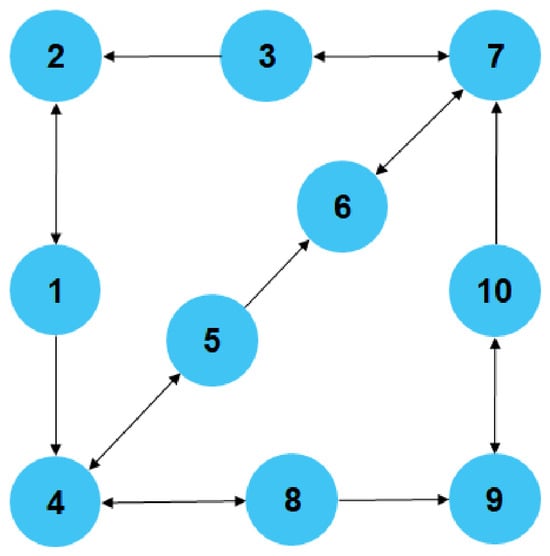
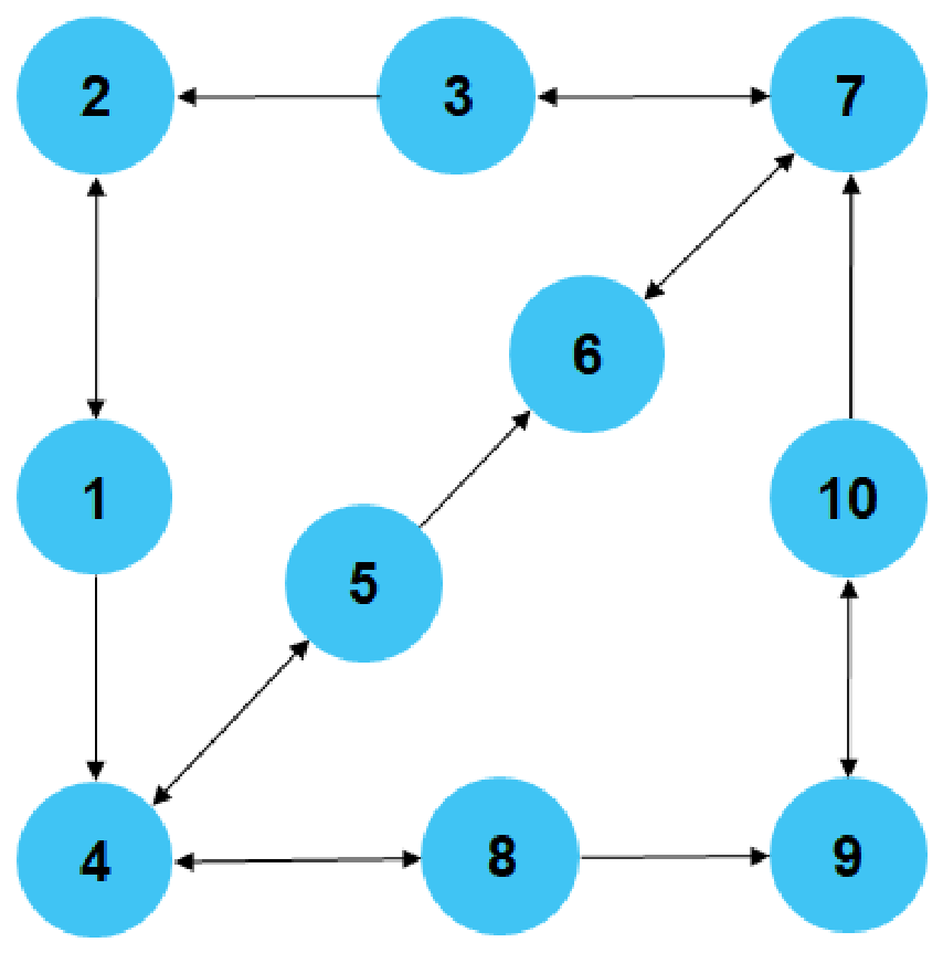
Here, $c=0.1$ is the fixed step-size scale used in the numerical study, giving an initial step size of ${\gamma }_0=0.1$. This scale has a precedent in distributed resource optimization: Hao et al. [34] use the diminishing subgradient step size $v^k=0.1/\sqrt{k}$, which has the same form after reindexing $k=t+1$. For the same one-point gradient estimate, the factor $0.1$ makes the gradient-based correction one tenth of that under the unit-scale schedule $1/\sqrt{t+1}$, thereby moderating the update magnitude. The coefficient controls the scale of the update, whereas the denominator controls its inverse-square-root decay; $0.1$ is therefore a numerator coefficient. It is a literature-supported numerical setting, not an optimal or universal constant. The regret bounds in Section 3 are written for unit scale; a fixed positive scale changes the constants associated with ${\sum }_t{\gamma }_t$ and $1/{\gamma }_T$, but not their $\sqrt{T}$ order. The scheduled grid exchange is set to $p_t^{\mathrm{grid}}=0$ in the reported case, and the initial conventional outputs sum to the initial risk-aware net demand. Figure 1 shows the strongly connected communication topology. The row-stochastic matrix $A_r$ and column-stochastic matrix $A_c$ are constructed as

$$\begin{array}{c}\hfill {\left[A_r\right]}_{ij}=\left\{\begin{array}{ccc}{\displaystyle \frac{1}{d_{i,\mathrm{in}}}},\hfill & \hfill & j\in {\mathcal{N}}_i^{\mathrm{in}},\hfill \\ 0,\hfill & \hfill & j\notin {\mathcal{N}}_i^{\mathrm{in}},\hfill \end{array}\right.\end{array}$$

(80)

and

$$\begin{array}{c}\hfill {\left[A_c\right]}_{ij}=\left\{\begin{array}{ccc}{\displaystyle \frac{1}{d_{j,\mathrm{out}}}},\hfill & \hfill & i\in {\mathcal{N}}_j^{\mathrm{out}},\hfill \\ 0,\hfill & \hfill & i\notin {\mathcal{N}}_j^{\mathrm{out}},\hfill \end{array}\right.\end{array}$$

(81)

where ${\mathcal{N}}_i^{\mathrm{in}}$ denotes the in-neighbor set of DG i, ${\mathcal{N}}_j^{\mathrm{out}}$ denotes the out-neighbor set of DG j, and $d_{i,\mathrm{in}}$ and $d_{j,\mathrm{out}}$ represent the corresponding in-degree and out-degree, respectively.

Figure 1. Communication topology diagram for 10 DGs.

4.2. Probabilistic PV Forecasting and Risk-Aware Demand

The evaluated forecasting sequence contains the actual PV output $p_{pv}^t$, the median forecast ${\widehat{p}}_{pv}^{\left(0.5\right),t}$, and the lower and upper quantiles ${\widehat{p}}_{pv}^{\left(\alpha \right),t}$ and ${\widehat{p}}_{pv}^{(1-\alpha ),t}$. In the reported case study, the lower-tail risk parameter is fixed at $\alpha =0.05$ before the online dispatch process. Accordingly, the fifth-percentile PV forecast is used as the lower forecast bound, corresponding to a nominal lower-side reliability of $1-\alpha =0.95$. Together with the upper quantile ${\widehat{p}}_{pv}^{\left(0.95\right),t}$, it forms a central prediction interval with a nominal coverage of $1-2\alpha =0.90$. This setting is adopted to provide protection against PV underproduction without introducing an excessively conservative reserve requirement.

The interval between two consecutive samples is 5 min; therefore, each complete day contains 288 samples. The time axes in the PV forecasting and prediction-interval figures use this same sampling interval.

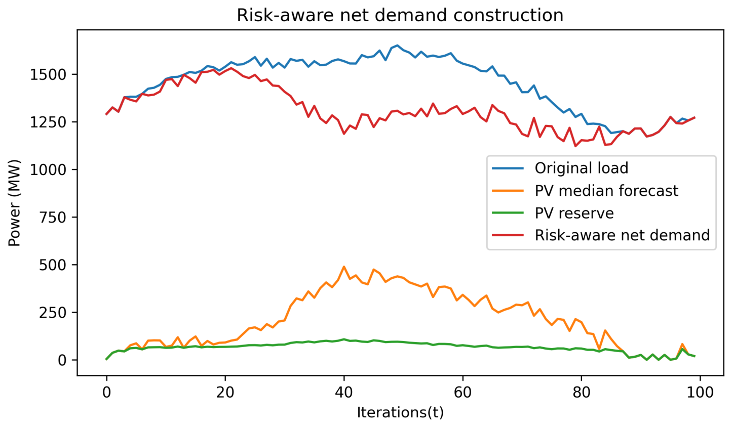
The lower-side reserve is computed as

$$R_{pv}^t={\left[{\widehat{p}}_{pv}^{\left(0.5\right),t}-{\widehat{p}}_{pv}^{\left(\alpha \right),t}\right]}_{+}.$$

Accordingly, the dispatch target is transformed from the original load demand $p_D^t$ into the risk-aware net demand

$$P_{\mathrm{net}}^t=p_D^t-{\widehat{p}}_{pv}^{\left(0.5\right),t}+R_{pv}^t.$$

The conventional DGs therefore track $P_{\mathrm{net}}^t$ rather than the original load $p_D^t$.

To further characterize the meteorological information contained in $X_t$, a supplementary correlation analysis was performed using the 5 min PV and meteorological measurements from the DKASC Alice Springs DKA-M5 C-Phase data over 2020–2022. To avoid artificially increasing the correlations because of the large number of simultaneous zero-PV and zero-irradiance observations during nighttime, only daylight samples satisfying $G_t^{\mathrm{GHI}}>20\mathrm{W}/{\mathrm{m}}^2$ and $p_{pv}^t>0.01\mathrm{kW}$ were retained. This resulted in 138,048 valid samples. Both Pearson and Spearman correlation coefficients were calculated to quantify, respectively, the linear and monotonic associations between each meteorological variable and the measured PV output. The results are reported in Table 4.

Table 4. Correlation between meteorological input features and measured PV output.

Meteorological Feature	Pearson r	Spearman $\mathit{\rho }$
Global tilted irradiance (GTI)	0.9811	0.9814
Global horizontal irradiance (GHI)	0.9626	0.9656
Diffuse horizontal irradiance (DHI)	0.1503	0.3829
Ambient temperature	0.2066	0.1965
Relative humidity	$-0.3387$	$-0.2731$

As shown in Table 4, GTI and GHI exhibit the strongest positive associations with the measured PV output, with Pearson coefficients of 0.9811 and 0.9626, respectively. Their corresponding Spearman coefficients are also high, indicating that these relationships remain strong under a rank-based measure. Relative humidity exhibits a negative association with PV generation, whereas DHI and ambient temperature show weaker marginal correlations. These pairwise coefficients are used to characterize the association of individual meteorological variables with PV output rather than to represent model-specific feature importance; weaker pairwise correlation does not imply that a variable is uninformative within the nonlinear multivariate temporal forecasting model.

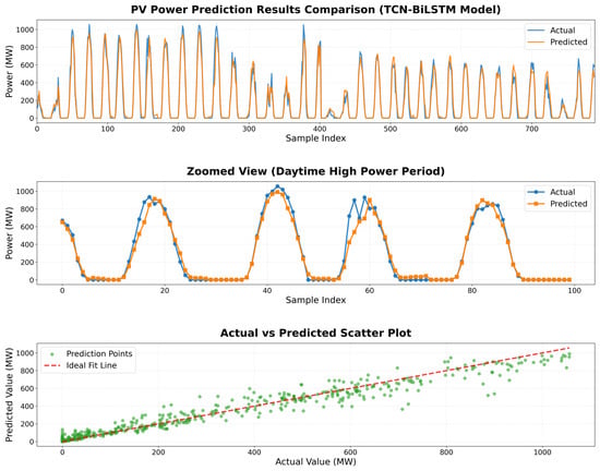
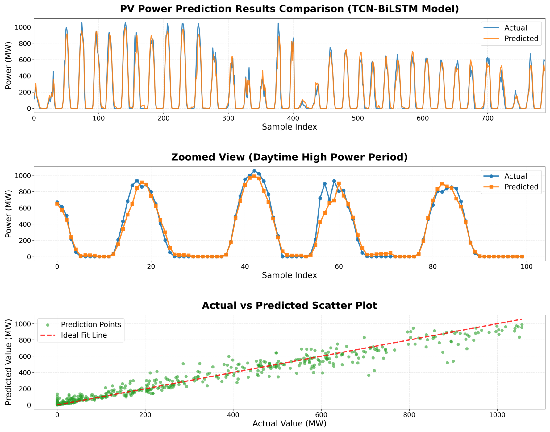
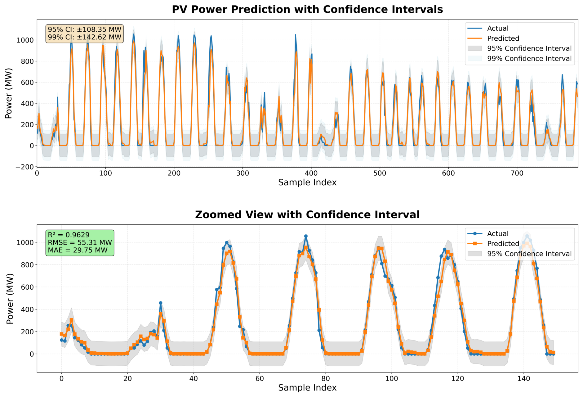
Figure 2 compares the TCN–BiLSTM prediction with the observed PV profile. On the evaluated sequence, the reported $R^2$, RMSE, and MAE are $0.9629$, $55.31$ MW, and $29.75$ MW, respectively. The enlarged region also shows visible errors during several rapid ramps, so the forecast is informative but not exact.

Figure 2. Prediction performance of the proposed TCN-BiLSTM-based PV forecasting model. The figure compares the actual PV output and predicted values, including the overall forecasting results, the enlarged daytime high-power period, and the actual-predicted correlation analysis.

To further validate the forecasting model, three representative baselines—ARIMA, CNN, and GRU—were implemented using the same dataset division and evaluation metrics. Table 5 reports the resulting RMSE, MAE, and pinball loss.

Table 5. Performance comparison among different forecasting models. Lower values indicate better performance.

Model	RMSE (MW)	MAE (MW)	Pinball Loss
ARIMA	112.64	78.35	0.0862
CNN	78.92	46.83	0.0527
GRU	66.45	36.91	0.0415
TCN–BiLSTM	55.31	29.75	0.0328

In this comparison, TCN–BiLSTM achieved the lowest error for all three metrics: its RMSE, MAE, and pinball loss were 55.31 MW, 29.75 MW, and 0.0328, respectively. These results support the use of the hybrid architecture for the evaluated sequence and are consistent with its design rationale: the TCN extracts multi-scale temporal patterns, whereas the BiLSTM represents bidirectional temporal dependencies. The comparison is limited to the reported dataset split and does not establish universal superiority across sites or operating conditions.

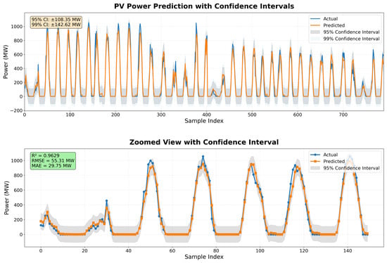
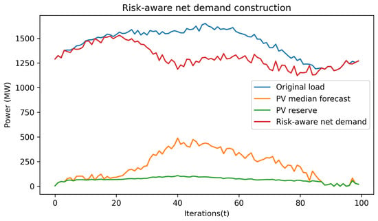
Figure 3 visualizes the associated prediction bands. These bands are used as an uncertainty diagnostic; the dispatch reserve itself is computed from the lower quantile in (13). Figure 4 then shows the resulting forecast-to-dispatch mapping. The median forecast lowers the conventional-generation requirement, whereas $R_{pv}^t$ partially offsets that reduction when lower-tail uncertainty is larger. The horizontal axis in Figure 4, Figure 5, Figure 6, Figure 7, Figure 8, Figure 9 and Figure 10 is labeled Iterations(t), where t is the dispatch iteration index.

Figure 3. Probabilistic PV forecasts and prediction intervals generated by the TCN–BiLSTM model. The intervals characterize the uncertainty range used to construct the lower-side dispatch reserve.

Figure 4. Construction of the risk-aware net demand under probabilistic PV forecasting.

4.3. Dispatch Tracking and Low-Carbon Performance

Figure 5 shows the output trajectories of the 10 conventional generators. All reported trajectories remain within the limits in Table 3 and respond to the time-varying dispatch target despite perturbations in the exchanged states.

Figure 5. Output power trajectories of conventional generators under probabilistic PV forecasting-driven dispatch.

Figure 5. Output power trajectories of conventional generators under probabilistic PV forecasting-driven dispatch.

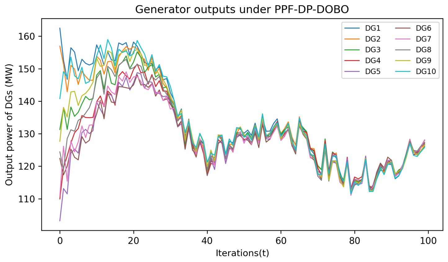
Because the load, PV contribution, and queried operating costs vary with time, the optimal dispatch is a time-indexed trajectory rather than a single static vector of generator outputs. Table 3 reports the cost coefficients and admissible output range of each controllable DG, while Figure 5 reports the corresponding optimized power trajectories over the evaluated horizon. PV is not optimized as an additional DG; its forecasted aggregate contribution is incorporated through $P_{\mathrm{net}}^t$.

Figure 6 compares aggregate conventional generation with $P_{\mathrm{net}}^t$. The two curves are visually coincident in the reported zero-grid-exchange case, showing that the balance-feasible schedule follows the target constructed from the median forecast and reserve. This experiment verifies numerical tracking for the tested profile; it does not by itself establish robustness to unmodeled network or device constraints.

Figure 6. Supply–demand balance between total conventional generation and risk-aware net demand.

Figure 6. Supply–demand balance between total conventional generation and risk-aware net demand.

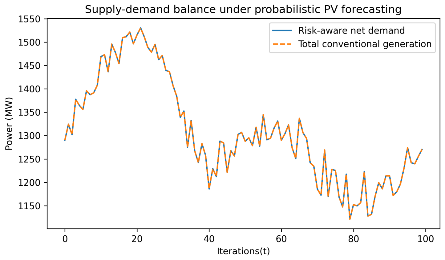
Figure 7 and Figure 8 present the with-PV and without-PV comparisons for the modified IEEE 162-bus dispatch case introduced in Section 4.1. The no-PV scenario requires the conventional DGs to meet the original load demand. The deterministic-PV scenario subtracts the median PV forecast from the load, without adding an uncertainty reserve. The probabilistic-PV scenario uses the median forecast together with the lower-side reserve to define the risk-aware net demand. Thus, the no-PV curve is the common baseline for the two PV-assisted scenarios in both figures. These are comparisons within the aggregate economic-dispatch model; they do not constitute a bus-level power-flow validation.

Figure 7. Average dynamic regret for the no-PV, deterministic-PV, and probabilistic-PV scenarios in the modified IEEE 162-bus dispatch case.

Figure 7. Average dynamic regret for the no-PV, deterministic-PV, and probabilistic-PV scenarios in the modified IEEE 162-bus dispatch case.

Figure 8. Carbon-trading costs for the no-PV, deterministic-PV, and probabilistic-PV scenarios in the modified IEEE 162-bus dispatch case.

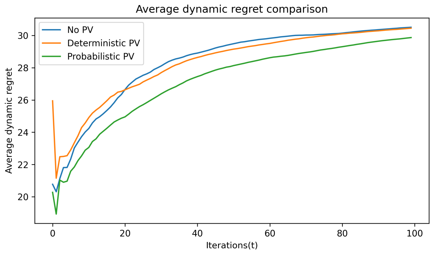
Figure 8. Carbon-trading costs for the no-PV, deterministic-PV, and probabilistic-PV scenarios in the modified IEEE 162-bus dispatch case.

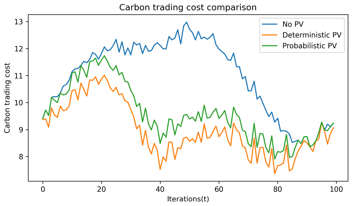
Figure 7 compares the reported average-regret values for the three scenarios. Over the displayed 100 iterations, all three curves increase and begin to flatten; therefore, this finite-horizon plot should not be described as evidence of decreasing average regret. The probabilistic-PV curve remains below the no-PV and deterministic-PV curves throughout most of the evaluated horizon. The asymptotic $\mathcal{O}\left(T^{3/4}\right)$ statement follows from Corollary 1 under its path-variation and forecasting-uncertainty conditions, rather than from this finite simulation alone.

Figure 8 shows that both PV-assisted cases reduce carbon-trading cost relative to the no-PV case over most of the horizon. The deterministic-PV case is usually lowest because it carries no lower-tail reserve. The probabilistic-PV case incurs a moderate reserve-related cost but remains below the no-PV case, illustrating the economic trade-off between renewable utilization and protection against PV underproduction.

4.4. Online Optimization and Privacy–Performance Trade-Off

Figure 9 compares PPF-DP-DOBO with RGF-DPGD [14], D-DPS [35], and D-OOA [36]. D-DPS uses exact gradients, RGF-DPGD uses two function queries, and D-OOA and PPF-DP-DOBO use one. The exact-gradient and two-point methods show faster finite-horizon reduction in regret. The proposed method pays an additional performance cost for Laplace perturbation, but it requires only one function query and protects released states. The comparison therefore illustrates an information–privacy–performance trade-off rather than uniform dominance over all baselines.

Figure 9. Average individual dynamic regret over time for the proposed method, RGF-DPGD, D-DPS, and D-OOA.

Figure 9. Average individual dynamic regret over time for the proposed method, RGF-DPGD, D-DPS, and D-OOA.

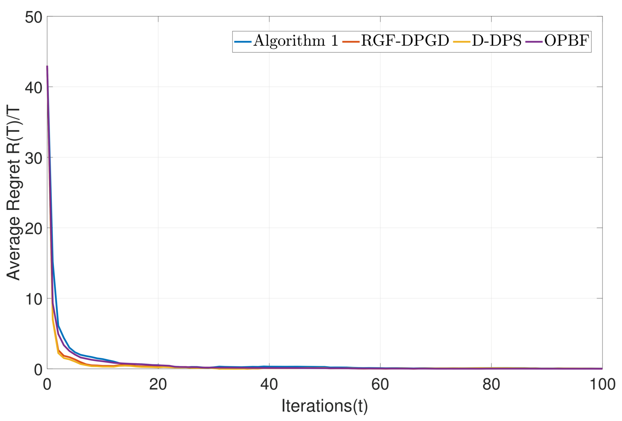
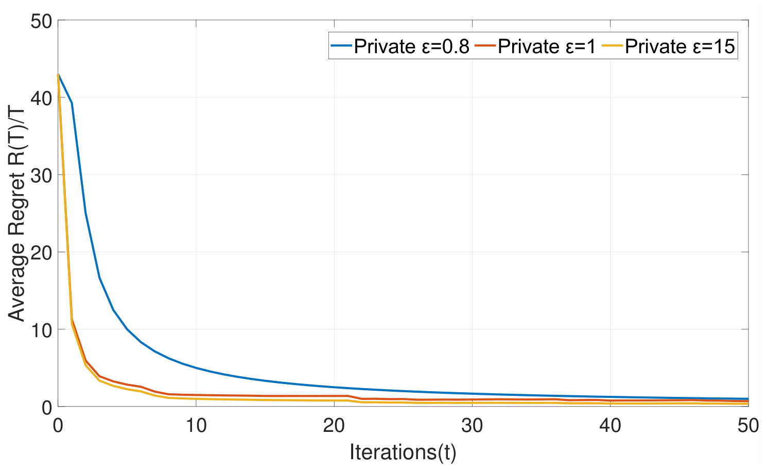
Figure 10 varies the constant per-release budget ${\epsilon }_t=\epsilon$. A larger value reduces the Laplace scale and improves the reported regret, but it weakens privacy. By Theorem 1, the corresponding horizon-level budget is $(T+1)\epsilon$ unless a nonuniform budget schedule or another composition strategy is used. Privacy parameters should therefore be selected at the horizon level rather than interpreted only per iteration.

Figure 10. Impact of the privacy budget $\epsilon$ on the average dynamic regret over time.

Figure 10. Impact of the privacy budget $\epsilon$ on the average dynamic regret over time.

To examine the sensitivity of PPF-DP-DOBO to the exploration radius and to determine whether a fixed radius remains appropriate when the generator capacity changes, an additional scale-sensitivity experiment is conducted. Since the same absolute exploration radius represents different relative perturbation magnitudes for generators with different operating ranges, we define the normalized exploration radius as

$$\overline{\delta }={\displaystyle \frac{\delta }{p_{i,\max }^{\left(s\right)}-p_{i,\min }^{\left(s\right)}}},$$

(82)

where s denotes the generator-scale factor. Three capacity scales, $s\in \{0.5,1,2\}$, are considered. For each scale, the generation limits and the corresponding risk-aware net demand are scaled consistently as $p_{i,\min }^{\left(s\right)}=s{p}_i^{\min }$, $p_{i,\max }^{\left(s\right)}=s{p}_i^{\max }$, and $P_{\mathrm{net}}^{t,\left(s\right)}=s{P}_{\mathrm{net}}^t$, while the generation-cost coefficients and the other algorithmic settings are kept unchanged. The normalized radii $\overline{\delta }\in \{0.05,0.10,0.25,0.50,0.75,0.90,1.00\}$ are evaluated, and each configuration is repeated over 20 independent random runs.

For cross-scale comparison, the cumulative dynamic regret is normalized by the cumulative magnitude of the corresponding optimal dispatch cost, i.e.,

$$\mathrm{NReg}\left(T\right)=100{\displaystyle \frac{\mathrm{Reg}\left(T\right)}{{\displaystyle {\displaystyle \sum _{t=1}^T}\left|{\displaystyle \sum _{i=1}^N}{f}_i^t\left(p_{i,t}^{\star }\right)\right|}}},$$

(83)

and is reported in percentage form.

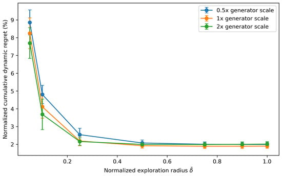
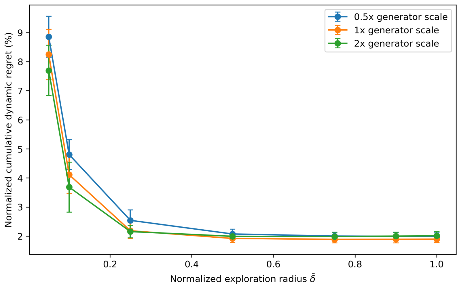
Figure 11 shows that the algorithm is sensitive to an excessively small exploration radius. For $\overline{\delta }=0.05$, the normalized cumulative dynamic regret is $8.8571\%$, $8.2467\%$, and $7.6956\%$ for the $0.5\times$, $1\times$, and $2\times$ generator scales, respectively. Increasing $\overline{\delta }$ to $0.25$ substantially reduces these values to $2.5412\%$, $2.1838\%$, and $2.1553\%$, respectively. The performance subsequently enters a broad low-regret region. At $\overline{\delta }=0.50$, the corresponding values are only $2.0726\%$, $1.9190\%$, and $1.9924\%$, and further increases in the normalized radius produce only small additional changes.

Figure 11. Sensitivity of the normalized cumulative dynamic regret to the normalized exploration radius under different generator scales. Error bars represent the mean ± standard deviation over 20 independent runs.

The results also show that a fixed absolute exploration radius is not scale invariant. In particular, the baseline value $\delta =1$ corresponds to normalized radii of approximately $0.00690$, $0.00345$, and $0.00172$ for the $0.5\times$, $1\times$, and $2\times$ cases, respectively, and produces normalized cumulative regrets of $19.3101\%$, $30.9603\%$, and $46.3544\%$. Hence, the same absolute value becomes progressively smaller relative to the generator operating range as the capacity scale increases. In contrast, scaling $\delta$ with the generator operating range produces similar low-regret behavior across the three cases.

The lowest observed regrets in the tested range occur at $\overline{\delta }=1.00$ for the $0.5\times$ case and at $\overline{\delta }=0.75$ for the $1\times$ and $2\times$ cases. However, the differences among the results for $\overline{\delta }\in [0.50,1.00]$ are small relative to the run-to-run variability. Therefore, these values should not be interpreted as unique global optima. Rather, the experiment indicates a broad low-regret region once a moderate normalized exploration radius is reached. This observation is also consistent with Corollary 1, where the theoretically balanced exploration radius depends on problem-dependent constants rather than being a universal fixed value.

Overall, the simulations support three bounded conclusions. First, probabilistic forecasts can be mapped to a risk-aware net demand that is tracked by the reported schedule. Second, PV-assisted cases reduce carbon-trading cost relative to the no-PV case, while the reserve adds cost relative to deterministic PV dispatch. Third, privacy perturbation and one-point feedback reduce the information requirement but slow finite-horizon optimization. The simulations do not establish the asymptotic regret rate, which remains a conditional theoretical result.

5. Discussion

The main contribution of PPF-DP-DOBO is the explicit coupling of learned temporal uncertainty with privacy-aware online control. The TCN–BiLSTM forecaster does not enter the dispatch recursion through its internal weights. Instead, its outputs are reduced to a median forecast and a lower-side reserve, which determine the risk-aware net demand. This modular interface makes the dispatch analysis applicable to another probabilistic forecaster if it supplies comparable quantiles and satisfies Assumption 5.

The results also expose three trade-offs. First, the lower-side reserve protects against PV underproduction but increases conventional generation relative to median-only dispatch. Second, one-point feedback reduces each update to one function query but converges more slowly than exact-gradient or two-point alternatives in the finite-horizon comparison. Third, stronger privacy requires more noise and therefore increases regret. These trade-offs are intrinsic to the problem and should not be interpreted as implementation defects.

From a practical perspective, these results provide several design implications for privacy-aware microgrid dispatch. First, the probabilistic PV forecasts are used not only as prediction outputs but also as an operational interface that converts lower-tail forecast uncertainty into a reserve-aware net-demand target. This allows the reserve level to respond to the predicted PV uncertainty instead of relying on a fixed deterministic margin. Second, the one-point bandit architecture requires only function-value feedback and is therefore relevant when analytical cost gradients are unavailable, expensive to evaluate, or undesirable to disclose. Third, the privacy-budget results indicate that privacy protection and dispatch performance should be configured jointly over the dispatch horizon, since stronger privacy increases the perturbation magnitude and may degrade finite-horizon performance. Finally, the exploration-radius sensitivity study shows that a fixed absolute exploration radius is not scale-invariant; therefore, the exploration parameter should be calibrated with respect to the generator operating range when the framework is transferred to systems with different capacity scales.

Several limitations define the scope of the conclusions. Although the updated forecasting evaluation includes ARIMA, CNN, and GRU baselines under the same dataset division, it remains limited to one site and one evaluated sequence and does not include a distribution-shift test or a broader multi-site benchmark. The forecasting experiment reports one evaluated sequence and does not provide a multi-site benchmark, distribution-shift test, or comparison with alternative probabilistic forecasters. Prediction-interval quality should also be assessed with empirical coverage and interval-width metrics in addition to point-forecast error. The dispatch study uses a modified IEEE 162-bus numerical case and omits network losses, line-flow constraints, generator ramp-rate limits, storage dynamics, demand response, and reactive power. Incorporating generator ramp-rate limits would introduce inter-temporal feasibility constraints because the admissible output at time t would depend on the generator output at time $t-1$. This extension would require a time-dependent feasible set and a corresponding extension of the present online regret analysis. Moreover, the reported simulation assumes balance-feasible schedules; a fully decentralized feasibility-restoration mechanism for detailed power-flow constraints is outside the present model. These modeling simplifications also imply several risks for practical deployment. Forecasting errors or poorly calibrated prediction intervals may lead to an inaccurate reserve requirement and consequently increase the risk of PV underproduction being insufficiently compensated. In addition, a dispatch schedule that is feasible under the present aggregate power-balance model may not remain physically feasible when network losses, line-flow limits, generator ramp-rate constraints, and other device dynamics are explicitly considered. The differential-privacy mechanism also introduces a privacy–performance trade-off, since stronger privacy requires larger perturbations and may increase finite-horizon dispatch error or regret. Therefore, the reported numerical results should be interpreted as evidence under the stated model assumptions rather than as a guarantee of identical economic or carbon-reduction performance in field operation.

The theoretical guarantees are conditional on convex bounded costs, a strongly connected directed communication graph, bounded sensitivity, controlled path variation, and controlled cumulative forecast uncertainty. The privacy guarantee is per release, and sequential composition causes the total pure-differential-privacy budget to grow over the horizon. Future work should therefore examine adaptive privacy-budget allocation, tighter composition, changing communication graphs, distributionally robust forecast-to-dispatch coupling, and network-constrained validation with real operational data.

6. Conclusions

This paper connected TCN–BiLSTM probabilistic PV forecasting with privacy-preserving distributed online low-carbon dispatch. The median forecast and lower quantile define a risk-aware net demand, while PPF-DP-DOBO combines one-point bandit feedback with Laplace-perturbed state exchange. The analysis provides a per-release differential privacy guarantee and a conditional $O\left(T^{3/4}\right)$ individual dynamic regret bound containing an explicit cumulative forecasting-uncertainty term. In the modified IEEE 162-bus dispatch case, Figure 5 and Figure 6 show that the reported probabilistic-PV schedules track the risk-aware target. The with-PV and without-PV comparisons are reported in Figure 7 and Figure 8: the probabilistic-PV scenario exhibits lower reported average regret over most of the evaluated horizon, and both PV-assisted scenarios exhibit lower carbon-trading costs than the no-PV baseline over most of that horizon. The method and privacy-budget comparisons in Figure 9 and Figure 10 show the expected query and privacy trade-offs.

From a practical perspective, the results indicate that probabilistic PV forecasts can be translated into reserve-aware dispatch targets, one-point feedback can support online optimization when analytical gradients are unavailable, and privacy and exploration parameters should be selected jointly with the acceptable dispatch-performance degradation and generator operating scale.

These findings should be interpreted within the stated convex online model and numerical setting rather than as direct field-deployment guarantees. The observed carbon-cost reductions are case-dependent, and broader practical conclusions require further validation under detailed network constraints, generator dynamics, forecast-distribution shifts, and real operational data.

References

- Cheng, J.; Wang, L.; Pan, T. Optimized Configuration of Distributed Power Generation Based on Multi-Stakeholder and Energy Storage Synergy. IEEE Access 2023, 11, 129773–129787. [Google Scholar] [CrossRef] [Scilit]
- El-Rifaie, A.M.; Shaheen, A.M.; Tolba, M.A.; Smaili, I.H.; Moustafa, G.; Ginidi, A.R.; Elshahed, M.A. Modified Gradient-Based Algorithm for Distributed Generation and Capacitors Integration in Radial Distribution Networks. IEEE Access 2023, 11, 120899–120917. [Google Scholar] [CrossRef] [Scilit]
- Han, H.; Chen, X.; Liu, Z.; Liu, Y.; Su, M.; Chen, S. A Completely Distributed Economic Dispatching Strategy Considering Capacity Constraints. IEEE J. Emerg. Sel. Top. Circuits Syst. 2021, 11, 210–221. [Google Scholar] [CrossRef] [Scilit]
- Sun, L.; An, W.; Chen, Y.; Zhao, P.; Ding, D. An Overview of Distributed Economic Dispatch of Microgrids: Advances and Challenges. Syst. Sci. Control Eng. 2025, 13, 2467077. [Google Scholar] [CrossRef] [Scilit]
- Amnuaypongsa, W.; Wangdee, W.; Songsiri, J. Probabilistic solar power forecasting using multi-objective quantile regression. In 2024 18th International Conference on Probabilistic Methods Applied to Power Systems (PMAPS); IEEE: Piscataway, NJ, USA, 2024; pp. 1–6. [Google Scholar]
- Wu, Y.-K.; Phan, Q.-T.; Lo, H.-Y.; Zhan, K.-C.; Tan, W.-S. Weighted Quantile Regression-based Probabilistic Forecasting for Solar Photovoltaic Systems. IEEE Trans. Ind. Appl. 2026, 62, 5699–5715. [Google Scholar] [CrossRef] [Scilit]
- Boroumandfar, G.; Khajehzadeh, A.; Eslami, M. A Single and Multiobjective Robust Optimization of a Microgrid in Distribution Network Considering Uncertainty Risk. Sci. Rep. 2024, 14, 28195. [Google Scholar] [CrossRef] [Scilit] [PubMed]
- Yan, J.; Cao, J.; Cao, Y. Distributed Continuous-Time Algorithm for Economic Dispatch Problem Over Switching Communication Topology. IEEE Trans. Circuits Syst. II Express Briefs 2021, 68, 2002–2006. [Google Scholar] [CrossRef] [Scilit]
- Guo, F.; Li, G.; Wen, C.; Wang, L.; Meng, Z. An Accelerated Distributed Gradient-Based Algorithm for Constrained Optimization with Application to Economic Dispatch in a Large-Scale Power System. IEEE Trans. Syst. Man Cybern. Syst. 2021, 51, 2041–2053. [Google Scholar] [CrossRef] [Scilit]
- Mi, Y.; Yuan, D.; Ratnam, E.L.; Verbic, G.; Shi, G. Distributed online algorithms for economic power dispatch. In 2025 IEEE 64th Conference on Decision and Control (CDC); IEEE: Piscataway, NJ, USA, 2025; pp. 7220–7225. [Google Scholar]
- Wei, M.; Yu, W.; Liu, H.; Chen, D. Byzantine-Resilient Distributed Bandit Online Optimization in Dynamic Environments. IEEE Trans. Ind. Cyber-Phys. Syst. 2024, 2, 154–165. [Google Scholar] [CrossRef] [Scilit]
- Yuan, D.; Hong, Y.; Ho, D.W.C.; Xu, S. Distributed Mirror Descent for Online Composite Optimization. IEEE Trans. Autom. Control 2021, 66, 714–729. [Google Scholar] [CrossRef] [Scilit]
- Li, J.; Li, C.; Yu, W.; Zhu, X.; Yu, X. Distributed Online Bandit Learning in Dynamic Environments Over Unbalanced Digraphs. IEEE Trans. Netw. Sci. Eng. 2021, 8, 3034–3047. [Google Scholar] [CrossRef] [Scilit]
- Pang, Y.; Hu, G. Randomized Gradient-Free Distributed Optimization Methods for a Multiagent System with Unknown Cost Function. IEEE Trans. Autom. Control 2020, 65, 333–340. [Google Scholar] [CrossRef] [Scilit]
- Li, J.; Gu, C.; Wu, Z.; Huang, T. Online Learning Algorithm for Distributed Convex Optimization with Time-Varying Coupled Constraints and Bandit Feedback. IEEE Trans. Cybern. 2022, 52, 1009–1020. [Google Scholar] [CrossRef] [PubMed]
- Wang, C.; Xu, S.; Yuan, D.; Zhang, B.; Zhang, Z. Push-Sum Distributed Online Optimization with Bandit Feedback. IEEE Trans. Cybern. 2022, 52, 2263–2273. [Google Scholar] [CrossRef] [Scilit] [PubMed]
- Flaxman, A.D.; Kalai, A.T.; McMahan, H.B. Online Convex Optimization in the Bandit Setting: Gradient Descent Without a Gradient. arXiv 2004, arXiv:cs/0408007. [Google Scholar]
- Yuan, D.; Proutiere, A.; Shi, G. Distributed Online Optimization with Long-Term Constraints. IEEE Trans. Autom. Control 2022, 67, 1089–1104. [Google Scholar] [CrossRef] [Scilit]
- Yi, X.; Li, X.; Yang, T.; Xie, L.; Chai, T.; Johansson, K.H. Distributed Bandit Online Convex Optimization with Time-Varying Coupled Inequality Constraints. IEEE Trans. Autom. Control 2021, 66, 4620–4635. [Google Scholar] [CrossRef] [Scilit]
- Dwork, C. Differential Privacy. In International Colloquium on Automata, Languages, and Programming; Springer: Berlin/Heidelberg, Germany, 2006; pp. 1–12. [Google Scholar]
- Sun, L.; Ding, D.; Dong, H.; Bai, X. Privacy-Preserving Distributed Economic Dispatch for Microgrids Based on State Decomposition with Added Noises. IEEE Trans. Smart Grid 2023, 15, 2424–2433. [Google Scholar] [CrossRef] [Scilit]
- Zhao, D.; Liu, D.; Liu, L. Distributed Privacy Preserving Algorithm for Economic Dispatch Over Time-Varying Communication. IEEE Trans. Power Syst. 2024, 39, 643–657. [Google Scholar] [CrossRef] [Scilit]
- Lü, Q.; Deng, S.; Li, H.; Huang, T. Privacy Protection Decentralized Economic Dispatch Over Directed Networks with Accurate Convergence. IEEE Trans. Emerg. Top. Comput. Intell. 2023, 7, 1702–1716. [Google Scholar] [CrossRef] [Scilit]
- Xiong, Y.; Xu, J.; You, K.; Liu, J.; Wu, L. Privacy-Preserving Distributed Online Optimization Over Unbalanced Digraphs via Subgradient Rescaling. IEEE Trans. Control Netw. Syst. 2020, 7, 1366–1378. [Google Scholar] [CrossRef] [Scilit]
- Lian, Z.; Yu, H.; Chen, Y.; Shahidehpour, M.; Zhou, Q. Secure Microgrid Clusters Under Integrated Satellite–Terrestrial Networks: A Differential Privacy-Preserving Control Strategy. IEEE Trans. Ind. Electron. 2026, 73, 2104–2115. [Google Scholar] [CrossRef] [Scilit]
- Liu, J.; Ma, E.; Zha, L.; Tian, E. Distributed Energy Management for Microgrids: When Privacy Preservation Meets Multiple Mechanisms. IEEE Trans. Consum. Electron. 2026, 72, 1514–1523. [Google Scholar] [CrossRef] [Scilit]
- Yan, F.; Sundaram, S.; Vishwanathan, S.V.N.; Qi, Y. Distributed Autonomous Online Learning: Regrets and Intrinsic Privacy-Preserving Properties. IEEE Trans. Knowl. Data Eng. 2013, 25, 2483–2493. [Google Scholar] [CrossRef] [Scilit]
- Li, X.; Yi, X.; Xie, L. Distributed Online Optimization for Multi-Agent Networks with Coupled Inequality Constraints. IEEE Trans. Autom. Control 2020, 66, 3575–3591. [Google Scholar] [CrossRef] [Scilit]
- Huang, B.; Zou, Y.; Chen, F.; Meng, Z. Distributed Time-Varying Economic Dispatch via a Prediction-Correction Method. IEEE Trans. Circuits Syst. I Regul. Pap. 2022, 69, 4215–4224. [Google Scholar] [CrossRef] [Scilit]
- Lesage-Landry, A.; Callaway, D.S. Dynamic and Distributed Online Convex Optimization for Demand Response of Commercial Buildings. IEEE Control Syst. Lett. 2020, 4, 632–637. [Google Scholar] [CrossRef] [Scilit]
- Hosseini, S.; Chapman, A.; Mesbahi, M. Online Distributed Convex Optimization on Dynamic Networks. IEEE Trans. Autom. Control 2016, 61, 3545–3550. [Google Scholar] [CrossRef] [Scilit]
- Abdollahi, A.; Amato, G.; Savastio, L.P.; De Tuglie, E.E. A Game-Theoretic Optimization Framework for Secure and Cost-Efficient Dynamic Reconfiguration of Multi-microgrids. In Proceedings of the International Symposium on Intelligent Technology for Power and Energy Systems; Springer: Cham, Switzerland, 2026; pp. 21–35. [Google Scholar]
- Chen, G.; Yang, Q. An ADMM-Based Distributed Algorithm for Economic Dispatch in Islanded Microgrids. IEEE Trans. Ind. Inform. 2018, 14, 3892–3903. [Google Scholar] [CrossRef] [Scilit]
- Hao, Y.; Ni, Q.; Li, H.; Hou, S. On the Energy and Spectral Efficiency Tradeoff in Massive MIMO Enabled HetNets with Capacity-Constrained Backhaul Links. IEEE Trans. Commun. 2017, 65, 4720–4733. [Google Scholar] [CrossRef] [Scilit]
- Xi, C.; Khan, U.A. Distributed Subgradient Projection Algorithm Over Directed Graphs. IEEE Trans. Autom. Control 2017, 62, 3986–3992. [Google Scholar] [CrossRef] [Scilit]
- Zhao, Z.; Xia, L.; Jiang, L.; Ge, Q.; Yu, F. Distributed Bandit Online Optimisation for Energy Management in Smart Grids. Int. J. Syst. Sci. 2023, 54, 2957–2974. [Google Scholar] [CrossRef] [Scilit]
Disclaimer/Publisher’s Note: The statements, opinions and data contained in all publications are solely those of the individual author(s) and contributor(s) and not of MDPI and/or the editor(s). MDPI and/or the editor(s) disclaim responsibility for any injury to people or property resulting from any ideas, methods, instructions or products referred to in the content. |
© 2026 by the authors. Licensee MDPI, Basel, Switzerland. This article is an open access article distributed under the terms and conditions of the Creative Commons Attribution (CC BY) license.