Optimal Investment Control Under Jump-Fractional Dynamics: A Wick–Itô Approach

Abstract

This paper extends the optimal investment control framework by incorporating fractional Brownian motion to capture long-range dependence and memory effects in asset prices. Replacing the standard Brownian component with a fractional Brownian motion governed by the Hurst parameter H with $H\in (1/2,1)$, we employ the Wick–Itô calculus to derive the associated Hamilton–Jacobi–Bellman (HJB) equation. The resulting nonlinear PDE contains a time-dependent diffusion coefficient that reduces to the classical model when $H={\displaystyle \frac{1}{2}}$. We apply a linearized generalized Newton method to construct an iterative sequence for the value function and provide a numerical convergence analysis via the contraction mapping theorem. Using real GOOGL data, we obtain a model-implied mean optimal allocation of ${\overline{\pi }}^{*}=68.35\%$ for $H=0.62$, close to the classical $69.76\%$. A comprehensive sensitivity analysis identifies volatility $\sigma$ and jump intensity $\lambda$ as the dominant drivers of the optimal allocation, with absolute effects of $9.44\%$ and $6.47\%$, respectively, while the Hurst parameter H, the jump threshold $\tau$, and mean return $\alpha$ have smaller effects. The proposed framework provides a dynamic optimal investment ratio ${\pi }^{*}\left(t\right)$ that adjusts to market memory, offering a model-based strategy for portfolio management under both jump and long-memory risks. Empirical validation through backtesting is needed to establish its practical superiority.

1. Introduction

Optimal capital allocation in financial markets remains a central challenge in quantitative finance, requiring a delicate balance between maximizing returns and managing risks arising from volatility, price shocks, and structural changes in asset dynamics. While the classical Merton framework provides a foundational solution, its reliance on standard Brownian motion, which assumes independent and stationary increments, fails to capture empirical regularities such as long-range dependence, memory effects, and self-similarity observed in financial returns [1,2]. While our previous work [3] addressed this problem under the Merton jump-diffusion model, it did not account for the persistent memory effects that are the focus of the present paper.

1.1. From Classical to Fractional Framework

Our previous work [3] addressed the optimal investment problem under the Merton jump-diffusion (MJD) model [4,5]:

$$d{S}_t=(\alpha -\lambda k)S_{t}dt+\sigma S_{t}d{B}_t+(y_t-1)S_{t}d{N}_t,$$

(1)

leading to the nonlinear Hamilton–Jacobi–Bellman (HJB) equation:

$$v_t+rx{v}_x-{\displaystyle \frac{{\mathrm{\Delta }}^2{\left(v_x\right)}^2}{\mathrm{\Omega }{v}_{xx}}}=0,$$

(2)

with $\mathrm{\Delta }=\alpha -\lambda k-r$ and $\mathrm{\Omega }=2({\sigma }^2+\lambda {(y_t-1)}^2)$. These definitions are consistent with the fractional framework developed in Section 2.3. The Newton iteration $v_{n+1}=K{v}_n$ with:

$$K={\displaystyle \frac{-{\mathrm{\Delta }}^2+rx\mathrm{\Omega }+\mathrm{\Omega }}{2\mathrm{\Omega }+2rx\mathrm{\Omega }-2{\mathrm{\Delta }}^2}},$$

(3)

converges under $\left|K\right|<1$, yielding a constant optimal allocation ${\pi }^{*}\approx 70\%$ (more precisely, $69.76\%$) for GOOGL data in the classical case. In the fractional setting, the time derivative $v_t$ cannot be eliminated due to the time-dependent diffusion coefficient $2H{\sigma }^2{t}^{2H-1}$, leading to a time-dependent contraction factor $K\left(t\right)$ that simplifies algebraically to $K=1/2$ (see Section 3.2).

Remark on the jump term. 

We emphasize that the quadratic jump term that appears in the HJB equation is a second-order Taylor approximation of the exact finite-jump increment $\mathrm{\Delta }v=v(t,x(1+\pi q_t))-v(t,x)$, where $q_t=y_t-1$. This approximation is standard in the jump-diffusion literature for small jumps [2,3], and for the observed jump magnitudes in our dataset (largest jump $|q_t|=9.68\%$), the remainder of the Taylor expansion is of order ${10}^{-4}$, negligible compared to other terms. This modeling choice follows the deterministic-jump approach of [3], where jumps are treated as observed historical quantities rather than random variables and preserves the closed-form tractability of the optimal allocation and the contraction factor.

Remark on the value function. 

For the analytical derivation of the contraction factor $K\left(t\right)$, we follow [3] and use the separable test function $v(x,t)=e^{x+t}$, which renders $v_t=v_x=v_{xx}$ and enables a closed-form expression for $K\left(t\right)$. This function is used only as a computational device for deriving the contraction factor; the true value function for logarithmic utility has the form $v(t,x)=A\left(t\right)logx+B\left(t\right)$. For the numerical computation of the optimal allocation ${\pi }^{*}\left(t\right)$, we use the same test function $e^{x+t}$ for consistency with [3] and interpret the resulting allocation as a model-implied approximation. This modeling choice is deliberate and is clearly stated in Section 3.2.

Despite its success, this framework overlooks the persistent memory effects documented in financial markets. To address this limitation, we replace $B_t$ with fractional Brownian motion $B_t^H$, characterized by:

$$\mathbb{E}\left[B_t^H{B}_s^H\right]={\displaystyle \frac{1}{2}}\left(t^{2H}+s^{2H}-{|t-s|}^{2H}\right),$$

(4)

where $H\in (0,1)$ governs memory strength: $H>0.5$ indicates persistence, $H<0.5$ indicates anti-persistence, and $H=0.5$ recovers standard Brownian motion. In this work, we focus on the persistent regime $H\in (1/2,1)$, for which the standard Wick–Itô calculus with the kernel representation $\varphi (s,t)={H(2H-1)|s-t|}^{2H-2}$ is well-defined and the associated HJB equation can be rigorously derived. The anti-persistent regime $H<1/2$ would require an appropriate functional-analytic formulation (e.g., using fractional Sobolev spaces or Malliavin calculus) and remains an open direction for future work.

1.2. Related Literature and Research Gap

Recent literature has increasingly explored fractional Brownian motion in optimal portfolio selection. Yan [6] derived fractional HJB equations with time-dependent volatility ${\sigma }^2{t}^{2H-1}$, while Yaghobipour and Yarahmadi [7] developed numerical methods for stochastic-fractional optimal control problems with application in portfolio management. Han and Li [8] established stochastic maximum principles for fractional systems, and De Witte et al. [9] studied multivariate jump-diffusion optimization with SGD methods. Zongo and Nikiema [10] proved viscosity solution existence for fractional SABR models, and numerical approaches including deep FBSDE methods [11] and Bayesian inference [12] have been developed. Ban, He, and Liang [13] investigated optimal investment strategies for defined contribution pension schemes under partial information, highlighting the role of filtering techniques in fractional environments.

The combination of fractional Brownian motion with jump processes has been explored in various financial contexts. Yang [14] developed a pricing framework for American fractional lookback options in a mixed jump-diffusion fractional Brownian motion environment, utilizing the Wick–Itô-Skorokhod integral. In a related study, Yang [15] investigated optimal investment and life insurance strategies within a mixed jump-diffusion fractional framework, deriving closed-form solutions for CRRA utility preferences. More recently, Hu et al. [16] proposed a stock prediction model based on mixed fractional Brownian motion (MFBM), combining geometric Brownian motion and geometric fractional Brownian motion to capture both short-term and long-term dependencies. Ichiba, Pang, and Taqqu [17] examined the semimartingale properties of generalized fractional Brownian motion, with implications for asset pricing models. Additionally, Biagini and Øksendal [18] established fundamental results on minimal variance hedging for fractional Brownian motion using the Wick–Itô integral, while Narita [19] provided a comprehensive stochastic analysis framework for Black-Scholes markets driven by fractional Brownian motion.

While previous works such as Yan [6] derived the fractional HJB equation without jumps, and Yang [14,15] incorporated jumps in the context of option pricing and life insurance, none of these studies addressed the optimal investment allocation problem with both jumps and fractional dynamics in a unified framework. Our paper fills this gap by extending the classical MJD framework [3] to include fractional Brownian motion, deriving the corresponding HJB equation, and providing a numerical method with a time-dependent contraction factor. This combination of jumps, fractional dynamics, and dynamic optimal allocation is new to the literature.

1.3. Contributions and Paper Structure

The main contributions of this paper are:

• A generalized MJD model that combines both jumps and fractional Brownian motion in a unified framework for optimal portfolio control. Unlike Yan [6], who did not consider jumps, and Yang [14,15], who focused on option pricing and life insurance, we directly solve the optimal capital allocation problem.
• Derivation of the fractional HJB equation using Wick–Itô calculus with the time-dependent diffusion coefficient $2H{\sigma }^2{t}^{2H-1}$, which generalizes the jump version of Yan’s equation [6]. Unlike the classical MJD framework [3], where the test function $v(x,t)=e^{x+t}$ renders $v_t=v_x=v_{xx}$ and effectively eliminates the time derivative, in the fractional setting the time-dependent diffusion coefficient prevents such simplification. Consequently, the time derivative $v_t$ must be retained explicitly in the HJB equation, the Fréchet derivative, and the contraction factor $K\left(t\right)$.
• Introduction of a time-dependent contraction factor $K\left(t\right)$ that generalizes the classical convergence condition to ${sup}_t\left|K\left(t\right)\right|<1$, providing a practical numerical stability indicator for the Newton iteration. As shown in Section 3.2, this factor simplifies algebraically to $K=1/2$ across all parameter values and time steps, confirming the numerical robustness of the method.
• A dynamic optimal investment ratio ${\pi }^{*}\left(t\right)$ that adapts to market memory through $t^{2H-1}$.
• Numerical validation with real GOOGL data and a comprehensive sensitivity analysis with respect to all key parameters (H, $\sigma$, $\lambda$, $\alpha$), identifying volatility $\sigma$ and jump intensity $\lambda$ as the primary drivers of optimal allocation.
• The numerical stability condition ${sup}_t\left|K\left(t\right)\right|<1$, which provides a practical criterion for monitoring the convergence of the Newton iteration in fractional settings.

Remark on modeling choices. 

We emphasize two modeling choices that are made explicit throughout the paper. First, the jump term in the HJB equation is a second-order Taylor approximation of the exact finite-jump increment, standard in the jump-diffusion literature [2,3]; for the observed jump magnitudes, the approximation error is of order ${10}^{-4}$. Second, the separable test function $v(x,t)=e^{x+t}$ is used as a computational device for deriving the contraction factor and for computing the model-implied optimal allocation, following [3]; it is not the true value function, which for logarithmic utility has the form $v(t,x)=A\left(t\right)logx+B\left(t\right)$. These choices are clearly stated in Section 2.3 and Section 3.2.

The paper is organized as follows. Section 2 presents the mathematical model, including asset price dynamics, wealth process, and value function, along with the Wick–Itô stochastic calculus and the derivation of the fractional HJB equation. Section 3 formulates the generalized Newton method and provides a numerical convergence analysis via the contraction mapping theorem. Section 4 provides numerical implementation with real GOOGL market data and presents a comprehensive sensitivity analysis. Section 5 discusses the financial interpretation and model-implied practical implications for portfolio managers. Finally, Section 6 concludes the paper and outlines future research directions.

2. Mathematical Model

This section establishes the mathematical framework for optimal investment control under fractional Brownian motion with jumps. We define the asset price dynamics, derive the wealth process and value function, present the necessary stochastic calculus, derive the fractional HJB equation and optimal allocation, and finally connect the results to the classical model.

2.1. Asset Price Dynamics and Wealth Process

Let $(\mathrm{\Omega },\mathcal{F},\mathbb{P})$ be a complete probability space with a filtration ${\left\{{\mathcal{F}}_t\right\}}_{t\ge 0}$ satisfying the usual conditions. The risky asset price $S_t$ follows the Wick–Itô SDE:

$$d{S}_t=(\alpha -\lambda k)S_{t}dt+\sigma S_{t}d{B}_t^H+(y_t-1)S_{t}d{N}_t,$$

(5)

with parameters:

• $\alpha \in \mathbb{R}$: expected return (model parameter);
• $\sigma >0$: volatility;
• $\lambda >0$: jump intensity of Poisson process $N_t$;
• k: average jump size, defined as the sample mean $k={\displaystyle \frac{1}{n}}{\sum }_{t=1}^n(y_t-1)$ over the identified jump days;
• $y_t>0$: deterministic jump multiplier at time t;
• $B_t^H$: fractional Brownian motion with $H\in (1/2,1)$;
• $N_t$: Poisson process independent of $B_t^H$.

The jump sizes $\left\{y_t\right\}$ are treated as deterministic quantities extracted from historical data at specific points in time, not as random variables. Following the standard practice in the jump-diffusion literature [2,3], we identify jumps via the threshold rule $|R_t|>0.01$, where

$$R_t={\displaystyle \frac{S_t-S_{t-1}}{S_{t-1}}}$$

(6)

denotes the observed daily return at time t, and set $y_t=S_t/S_{t-1}$ for such days. Thus, each $y_t$ is an observed numerical value at a specific time point, and $y_t-1=R_t$ is the return at the jump time. This deterministic specification preserves the Markovian structure of the problem, as the jump component does not introduce additional randomness into the state beyond the current value $x_t$.

Remark on the deterministic-jump approach. 

We emphasize that this deterministic-jump approach follows [3] and differs from the standard Merton model with random jump times and sizes. In the standard Merton model, jumps occur at random times governed by a Poisson process, and their sizes are random variables (typically log-normally distributed). In contrast, our approach treats jumps as observed historical events at specific dates with specific magnitudes. This modeling choice is deliberate and is designed to study the effect of specific extreme events (such as the largest jump in the sample, occurring on day 228 with magnitude $9.68\%$) on the optimal allocation. It also preserves the closed-form tractability of the optimal allocation and the contraction factor, which is the primary focus of this paper.

Notation. 

In the sequel, we distinguish between the model parameter $\alpha$ (the expected return in the SDE (5)) and the observed daily return $R_t$ defined in (6). The parameter $\alpha$ is estimated as the sample mean $\overline{R}={\displaystyle \frac{1}{n}}{\sum }_{t=1}^n{R}_t$. This notation avoids the ambiguity present in [3], where the symbol ${\alpha }_t$ was used for the daily return and $\alpha$ for both the model parameter and the sample mean.

The Wick–Itô interpretation is essential since $B_t^H$ is not a semimartingale for $H\ne {\displaystyle \frac{1}{2}}$, as will be discussed in Section 2.2.

Consider a self-financing portfolio with a risk-free asset (rate $r>0$) and the risky asset $S_t$. Let ${\pi }_t$ be the fraction of wealth allocated to $S_t$. With zero consumption, the wealth process satisfies:

$$d{x}_t=x_t\left[\left(r+{\pi }_t(\alpha -\lambda k-r)\right)dt+{\pi }_t\sigma d{B}_t^H+{\pi }_t(y_t-1)d{N}_t\right],$$

(7)

where ${\pi }_t$ is ${\mathcal{F}}_t$-progressively measurable and satisfies the integrability condition:

$$\mathbb{E}\left[{\int }_0^T{\pi }_t^2{\sigma }^2{t}^{2H-1}dt\right]<\infty ,$$

(8)

ensuring the Wick–Itô integral in (7) is well-defined. The admissible set $\mathcal{A}$ also includes the wealth positivity condition:

$$1+{\pi }_t(y_t-1)>0\mathrm{almost}\mathrm{surely},\mathrm{for}\mathrm{all}t,$$

(9)

which ensures that $x_t>0$ almost surely, necessary for the logarithmic utility $log\left(x_T\right)$ to be well-defined.

The investor maximizes expected logarithmic utility from terminal wealth:

$$v(t,x)=\underset{{\pi }_t\in \mathcal{A}}{max}\mathbb{E}\left[log\left(x_T\right)\mid x_t=x\right],$$

(10)

where $\mathcal{A}$ denotes the set of admissible controls satisfying (8), (9), and the standard measurability conditions. The logarithmic utility is chosen for analytical tractability and its constant relative risk aversion (CRRA) property with a coefficient of one.

We note that while the underlying fractional Brownian motion is non-Markovian, the value function retains the Markovian form $v(t,x)$ due to the special properties of the Wick–Itô calculus and the deterministic nature of the jump sizes $\left\{y_t\right\}$. Specifically, the Wick–Itô integral of deterministic integrands has zero unconditional expectation, and the controlled state dynamics depend on the past only through the current state $x_t$ and the deterministic coefficient $2H{\sigma }^2{t}^{2H-1}$. This property is specific to the Wick–Itô framework and differs from the classical conditional expectation; we refer the reader to Section 2.2 and [20] for a rigorous treatment. The memory of the fractional process enters the problem through the time-dependent diffusion coefficient $2H{\sigma }^2{t}^{2H-1}$, which is a deterministic function of time.

A key feature of our framework is its consistency with classical results. When $H={\displaystyle \frac{1}{2}}$, the fractional Brownian motion $B_t^{1/2}$ reduces to standard Brownian motion $B_t$, and the Wick–Itô integral coincides with the classical Itô integral. Consequently, (5) reduces to the classical MJD model [3]:

$$d{S}_t=(\alpha -\lambda k)S_{t}dt+\sigma S_{t}d{B}_t+(y_t-1)S_{t}d{N}_t,$$

(11)

which is identical to (1) in the Introduction. Similarly, the wealth dynamics (7) reduce to the standard self-financing condition. This ensures that our generalized framework contains the classical model as a special case, enabling direct comparison and validation.

2.2. Stochastic Calculus with Fractional Brownian Motion

Standard Itô calculus is not applicable to fractional Brownian motion. This subsection provides the necessary mathematical background for deriving the HJB equation in the fractional setting.

We emphasize that our use of the Wick–Itô calculus is specifically motivated by the optimal control nature of our problem. Unlike derivative pricing, where alternative fractional Itô formulae (based on Malliavin calculus) are often employed, the Wick–Itô framework is the standard and appropriate choice for deriving HJB equations in fractional optimal control problems [6,7,20].

For $H\ne {\displaystyle \frac{1}{2}}$, $B_t^H$ is neither a semimartingale nor a Markov process, rendering the classical Itô integral undefined and the standard dynamic programming principle inapplicable. To address this, we employ the Wick–Itô integral [20], which offers:

• Zero mean:$\mathbb{E}\left[{\int }_0^{T}f\left(s\right)d{B}_s^H\right]=0$ for suitable integrands.
• Isometry:

  $$\mathbb{E}\left[{\left({\int }_0^{T}f\left(s\right)d{B}_s^H\right)}^2\right]={\int }_0^T{\int }_0^{T}f\left(s\right)f\left(t\right)\varphi (s,t)dsdt,$$

  (12)

  with $\varphi (s,t)={H(2H-1)|s-t|}^{2H-2}$, which is well-defined and integrable for $H\in (1/2,1)$.
• No-arbitrage preservation in fractional Black–Scholes markets [20].

We emphasize that the no-arbitrage property in our framework is established in the Wick–Itô sense, which differs from the classical semimartingale notion. Specifically, the wealth process and trading gains are defined using the Wick–Itô integral, and the admissible strategies are those satisfying the integrability condition (8). Under these conventions, the fractional Black–Scholes market is arbitrage-free in the sense established by Biagini and Øksendal [18].

It is important to note that the Wick–Itô integral differs fundamentally from the classical semimartingale Itô integral. While the Wick–Itô integral preserves zero mean and provides a natural extension of the Itô theory to non-semimartingale processes, it does not share all properties of the semimartingale integral. In particular, the usual self-financing trading condition must be reinterpreted in the Wick–Itô sense, and the absence of arbitrage holds only under the weaker fractional Brownian notion, not in the classical semimartingale sense. These distinctions are crucial for the financial interpretation of our model.

An important consequence of this property is that the Wick–Itô integral of deterministic integrands has zero unconditional expectation, which is used in the derivation of the HJB equation. We emphasize that this property is distinct from the classical conditional expectation: the Wick–Itô integral is defined through the Wick product, and its properties differ from those of the semimartingale integral. This distinction is essential for the correct interpretation of the Markovian reduction, and we refer the reader to [20] for a rigorous treatment of the Wick–Itô framework.

For $B_t^H$, the covariance of increments is $\mathbb{E}\left[d{B}_t^{H}d{B}_s^H\right]=\varphi (s,t)dtds$, where $\varphi (s,t)={H(2H-1)|s-t|}^{2H-2}$ for $H\in (1/2,1)$. In the Wick–Itô calculus, we define the correction term corresponding to the quadratic variation as:

$${\left(d{B}_t^H\right)}^2=2H{t}^{2H-1}dt.$$

(13)

Here, the equality is understood as a notational convention within the Wick–Itô framework, not as a classical pathwise quadratic variation. This is a pivotal result: for $H={\displaystyle \frac{1}{2}}$, we recover ${\left(d{B}_t\right)}^2=dt$; for $H\in (1/2,1)$, the time-dependent term $t^{2H-1}$ captures the memory effect.

Remark 1. 

For $H>1/2$, the fractional Brownian motion has vanishing classical pathwise quadratic variation (i.e., the limit of the sum of squared increments is zero). Therefore, the differential notation ${\left(d{B}_t^H\right)}^2=2H{t}^{2H-1}dt$ should not be interpreted as a classical quadratic variation; rather, it represents the correction term arising from the derivative of the covariance function in the Wick–Itô formula. This distinction is essential because the Wick–Itô integral is not a semimartingale integral for $H\ne 1/2$. In this work, we restrict our analysis to $H\in (1/2,1)$, for which the kernel $\varphi (s,t)$ is integrable and the standard Wick–Itô framework applies. We refer the reader to [20,21] for a rigorous treatment of the Wick–Itô integral and its properties.

For $g(t,x)\in C^{1,2}([0,T]\times \mathbb{R})$, the Wick–Itô formula takes the classical form:

$$dg(t,x_t)=g_{t}dt+g_{x}d{x}_t+{\displaystyle \frac{1}{2}}{g}_{xx}{\left(d{x}_t\right)}^2,$$

(14)

but with ${\left(d{x}_t\right)}^2$ computed using (13).

Using the wealth dynamics (7) and the fractional quadratic variation rule (13), along with the jump process properties (${\left(d{N}_t\right)}^2=d{N}_t$, $d{B}_t^H·d{N}_t=0$, $d{B}_t^H·dt=0$, $dt·d{N}_t=0$, ${\left(dt\right)}^2=0$), we obtain:

$$\begin{array}{cc}\hfill {\left(d{x}_t\right)}^2& =x_t^2{\left({\pi }_t\sigma d{B}_t^H+{\pi }_t(y_t-1)d{N}_t\right)}^2\hfill \\ \hfill & =x_t^2\left(2H{\pi }_t^2{\sigma }^2{t}^{2H-1}dt+{\pi }_t^2{(y_t-1)}^{2}d{N}_t\right).\hfill \end{array}$$

(15)

This fundamental result distinguishes the fractional model from the classical one: the term $2H{t}^{2H-1}$ captures the memory effect through the Hurst parameter H. For $H={\displaystyle \frac{1}{2}}$, we recover the classical quadratic variation ${\left(d{x}_t\right)}^2=x_t^2({\pi }_t^2{\sigma }^{2}dt+{\pi }_t^2{(y_t-1)}^{2}d{N}_t)$ from [3].

Remark 2. 

The time-dependent variance rate $2H{\sigma }^2{t}^{2H-1}$ reflects the non-Markovian nature of the system. For persistent markets ($H>0.5$), uncertainty grows with time.

2.3. Derivation of the Fractional HJB Equation

Although fractional Brownian motion is non-Markovian, the dynamic programming principle can still be applied in the Wick–Itô framework. The reduction to a Markovian value function $v(t,x)$ is justified by the following theorem, which we state explicitly.

Theorem 1 

(Markovian reduction for fractional control). Consider the optimal control problem with state dynamics driven by a Wick–Itô integral with respect to fractional Brownian motion $B_t^H$ with $H\in (1/2,1)$. Suppose that:

• The admissible controls ${\pi }_t$ are bounded and satisfy the integrability condition $\mathbb{E}\left[{\int }_0^T{\pi }_t^2{\sigma }^2{t}^{2H-1}dt\right]<\infty$;
• The Wick–Itô integral of deterministic integrands has zero unconditional expectation, and its properties differ from those of the classical conditional expectation (see Section 2.2 and [20] for a rigorous treatment);
• The controlled state dynamics depend on the past only through the current state $x_t$ and the deterministic time-dependent coefficient $2H{\sigma }^2{t}^{2H-1}$.

Then the value function can be written as $v(t,x)$, depending only on the current time t and the current state x, and the standard two-variable dynamic programming principle applies. This result follows from the Wick–Itô framework developed in [20] and is applied in the fractional optimal control literature [6,7].

All three hypotheses are satisfied in our jump-fractional model: (i) the admissible controls belong to the set $\mathcal{A}$ defined in Section 2.1, which includes the integrability condition (8) and the wealth positivity condition (9); (ii) the zero unconditional expectation property holds for the Wick–Itô integral (see Section 2.2); and (iii) the controlled state dynamics (7) depend on the past only through $x_t$ and the deterministic coefficient $2H{\sigma }^2{t}^{2H-1}$. The deterministic jump component, with jump sizes $y_t$ occurring at specific time points, preserves the Markovian structure because the jumps are determined by observed historical data and do not introduce additional randomness into the state beyond the current value $x_t$. This is a key feature of the deterministic-jump approach of [3], which differs from the standard Merton model with random jump times and sizes.

We now derive the HJB equation for the optimal investment problem using the Wick–Itô calculus and the dynamic programming principle.

Applying the Wick–Itô formula (14) to $v(t,x_t)\in C^{1,2}([0,T]\times {\mathbb{R}}^{+})$ with wealth dynamics (7) and quadratic variation (15):

$$\begin{array}{cc}\hfill dv& =v_{t}dt+v_{x}d{x}_t+{\displaystyle \frac{1}{2}}{v}_{xx}{\left(d{x}_t\right)}^2\hfill \\ \hfill & =\left[v_t+x(r+{\pi }_t(\alpha -\lambda k-r))v_x+{\displaystyle \frac{1}{2}}{x}^2{\pi }_t^2\left(2H{\sigma }^2{t}^{2H-1}+\lambda {(y_t-1)}^2\right)v_{xx}\right]dt\hfill \\ \hfill & +x{\pi }_t\sigma v_{x}d{B}_t^H+x{\pi }_t(y_t-1)v_{x}d{N}_t+{\displaystyle \frac{1}{2}}{x}^2{\pi }_t^2{(y_t-1)}^2{v}_{xx}(d{N}_t-\lambda dt).\hfill \end{array}$$

(16)

We emphasize that the quadratic jump term ${\displaystyle \frac{1}{2}}\lambda {\pi }^2{x}^2{(y_t-1)}^2{v}_{xx}$ in (16) arises from a second-order Taylor approximation of the exact finite-jump increment $\mathrm{\Delta }v=v(t,x(1+\pi q_t))-v(t,x)$, where $q_t=y_t-1$. This approximation is standard in the jump-diffusion literature for small jumps [2,3].

For the observed jump magnitudes in our dataset (largest jump $|q_t|=9.68\%$), the remainder of the Taylor expansion is bounded by ${\displaystyle \frac{|\pi q_t{|}^3}{3(1-|\pi q_t{\left|\right)}^3}}$, which is of order ${10}^{-4}$ for the parameters considered, negligible compared to other terms.

We note that this approximation is not an additional assumption; it is a consequence of the deterministic-jump modeling approach adopted in [3], where jumps are treated as observed historical quantities rather than random variables. The quadratic form preserves the closed-form tractability of the optimal allocation and the contraction factor. The term ${\displaystyle \frac{1}{2}}\lambda {\pi }_t^2{x}^2{(y_t-1)}^2{v}_{xx}$ in (17) below follows from taking the conditional expectation $\mathbb{E}\left[d{N}_t\right]=\lambda dt$.

Taking conditional expectations $\mathbb{E}[·\mid x_t=x]$ with $\mathbb{E}\left[d{B}_t^H\right]=0$ and $\mathbb{E}\left[d{N}_t\right]=\lambda dt$:

$$\mathbb{E}\left[dv\right]=\left[v_t+x(r+{\pi }_t(\alpha -\lambda k-r))v_x+{\displaystyle \frac{1}{2}}{x}^2{\pi }_t^2\left(2H{\sigma }^2{t}^{2H-1}+\lambda {(y_t-1)}^2\right)v_{xx}\right]dt.$$

(17)

The dynamic programming principle yields the HJB equation:

$$v_t+rx{v}_x+\underset{{\pi }_t}{max}\left\{{\pi }_{t}x(\alpha -\lambda k-r)v_x+{\displaystyle \frac{1}{2}}{\pi }_t^2{x}^2\left(2H{\sigma }^2{t}^{2H-1}+\lambda {(y_t-1)}^2\right)v_{xx}\right\}=0.$$

(18)

This generalizes the classical HJB (2) by introducing the time-dependent diffusion coefficient $2H{\sigma }^2{t}^{2H-1}$, which captures the memory effect while preserving the jump structure.

Remark 3. 

The time-dependent coefficient makes the fractional HJB equation non-stationary, increasing analytical and numerical complexity but providing a more realistic representation of financial markets with long-range dependence.

Differentiating the expression inside the maximum operator in (18) with respect to ${\pi }_t$ yields the first-order condition:

$$x(\alpha -\lambda k-r)v_x+{\pi }_t{x}^2\left(2H{\sigma }^2{t}^{2H-1}+\lambda {(y_t-1)}^2\right)v_{xx}=0.$$

(19)

Solving for ${\pi }_t$ gives the time-dependent optimal allocation:

$${\pi }_t^{*}=-{\displaystyle \frac{(\alpha -\lambda k-r)v_x}{x\left(2H{\sigma }^2{t}^{2H-1}+\lambda {(y_t-1)}^2\right)v_{xx}}}.$$

(20)

This generalizes the classical result [3] by replacing the constant ${\sigma }^2$ with $2H{\sigma }^2{t}^{2H-1}$. For $H={\displaystyle \frac{1}{2}}$, we recover the classical constant allocation:

$${\pi }^{*}=-{\displaystyle \frac{(\alpha -\lambda k-r)v_x}{x\left({\sigma }^2+\lambda {(y_t-1)}^2\right)v_{xx}}}.$$

(21)

The key features of this dynamic strategy are as follows:

• Time-adaptation: Unlike the classical constant ${\pi }^{*}$, this ratio evolves with $t^{2H-1}$, adapting to market memory.
• Memory effect: For $H>0.5$, the denominator grows with time, reducing allocation as uncertainty accumulates.
• Jump risk: The term $\lambda {(y_t-1)}^2$ accounts for discontinuous price movements, reducing allocation when jump risk is high.
• Reward-to-risk: The numerator $\alpha -\lambda k-r$ represents excess return adjusted for jump risk, making ${\pi }_t^{*}$ a dynamic reward-to-risk ratio.

Remark 4. 

The concavity condition $v_{xx}<0$ for logarithmic utility ensures the second-order sufficiency condition $x^2(2H{\sigma }^2{t}^{2H-1}+\lambda {(y_t-1)}^2)v_{xx}<0$ is satisfied.

Substituting ${\pi }_t^{*}$ from (20) into (18) and simplifying yields the nonlinear PDE:

$$v_t+rx{v}_x-{\displaystyle \frac{{(\alpha -\lambda k-r)}^2{\left(v_x\right)}^2}{2\left(2H{\sigma }^2{t}^{2H-1}+\lambda {(y_t-1)}^2\right)v_{xx}}}=0.$$

(22)

This nonlinear second-order PDE features a time-dependent coefficient arising from the fractional Brownian motion. The nonlinearity ${\left(v_x\right)}^2/v_{xx}$ is characteristic of HJB equations arising from utility maximization problems.

For notational convenience, we define:

$$\mathrm{\Delta }=\alpha -\lambda k-r,$$

(23)

and

$$\mathrm{\Omega }\left(t\right)=2\left(2H{\sigma }^2{t}^{2H-1}+\lambda {(y_t-1)}^2\right).$$

(24)

In the classical MJD framework, these definitions reduce to the constant forms $\mathrm{\Delta }=\alpha -\lambda k-r$ and $\mathrm{\Omega }=2({\sigma }^2+\lambda {(y_t-1)}^2)$. With these definitions, multiplying both sides of (22) by $\mathrm{\Omega }\left(t\right)v_{xx}$ yields the compact operator form:

$$F\left(v\right):=\mathrm{\Omega }\left(t\right)v_t{v}_{xx}+rx\mathrm{\Omega }\left(t\right)v_x{v}_{xx}-{\mathrm{\Delta }}^2{\left(v_x\right)}^2=0,$$

(25)

subject to the terminal condition $v(T,x)=log\left(x\right)$.

Remark 5. 

The operator F is homogeneous of degree two: $F\left(cv\right)=c^{2}F\left(v\right)$. This property, inherited from logarithmic utility, facilitates the numerical solution.

2.4. Connection to the Classical HJB

For $H={\displaystyle \frac{1}{2}}$, we have $t^{2H-1}=1$, so $\mathrm{\Omega }\left(t\right)$ in (24) reduces to the constant $\mathrm{\Omega }=2({\sigma }^2+\lambda {(y_t-1)}^2)$. Consequently, the operator (25) and the optimal ratio (20) reduce to their classical counterparts:

$$F\left(v\right)=\mathrm{\Omega }{v}_t{v}_{xx}+rx\mathrm{\Omega }{v}_x{v}_{xx}-{\mathrm{\Delta }}^2{\left(v_x\right)}^2=0,$$

(26)

$${\pi }^{*}=-{\displaystyle \frac{(\alpha -\lambda k-r)v_x}{x\left({\sigma }^2+\lambda {(y_t-1)}^2\right)v_{xx}}}.$$

(27)

This confirms that our framework generalizes the classical model, recovering it when memory effects are absent.

3. Numerical Implementation

3.1. Generalized Newton Method and Fréchet Derivative

We now develop the numerical solution methodology for the nonlinear fractional HJB equation. The linearized generalized Newton method from [3] is extended to handle the time-dependent coefficient $\mathrm{\Omega }\left(t\right)$. Numerical methods for controlled Hamilton–Jacobi–Bellman PDEs in finance have been extensively studied [22]. The contraction condition ${sup}_t\left|K\left(t\right)\right|<1$ is presented as a practical numerical stability indicator, while the actual convergence of the Newton iteration for the discretized HJB problem with terminal condition is verified numerically in Section 4.2.

We emphasize that the wealth variable $x_t$ is normalized by dividing by 100, so that the normalized wealth $x_t^{\mathrm{norm}}=x_t/100$ is dimensionless. This normalization is essential for ensuring that the optimal allocation ${\pi }^{*}\left(t\right)$ is dimensionless and comparable across different scales. In the numerical implementation, we use $x_{228}^{\mathrm{norm}}=10.41$ for the representative day 228.

For the theoretical analysis, we consider the space of functions $v\in C^{1,2}([0,T]\times [x_{min},x_{max}])$ satisfying the terminal condition $v(T,x)=logx$ and appropriate boundary conditions at $x=x_{min}$ and $x=x_{max}$. The space is equipped with the standard supremum norm:

$${\parallel v\parallel }_{C^{1,2}}=max\left\{{\parallel v\parallel }_{\infty },\parallel v_t{\parallel }_{\infty },\parallel v_x{\parallel }_{\infty },{\parallel v_{xx}\parallel }_{\infty }\right\}.$$

The domain $[x_{min},x_{max}]$ is bounded with $0<x_{min}<x_{max}<\infty$, ensuring that the norm is well-defined. In the numerical implementation, we choose $x_{min}={10}^{-4}$ and $x_{max}={10}^4$, which are sufficiently far from the regions where the solution is affected by the boundary conditions.

We solve $F\left(v\right)=0$ using the Newton iteration in Banach space [23]:

$$v_{n+1}=v_n-{\left[F^{\prime }\left(v_n\right)\right]}^{-1}F\left(v_n\right),$$

(28)

or equivalently, $F^{\prime }\left(v_n\right)(v_{n+1}-v_n)=-F\left(v_n\right)$, where $F^{\prime }\left(v_n\right)$ is the Fréchet derivative of F at $v_n$. The Newton iteration is applied with the terminal condition $v_{n+1}(T,x)=logx$.

Definition 1 

(Fréchet Derivative). Let $V,W$ be Banach spaces and $F:V\to W$. The operator F is Fréchet differentiable at $u_0\in V$ if there exists a bounded linear operator $A\in \mathcal{L}(V,W)$ such that:

$$F(u_0+h)=F\left(u_0\right)+Ah+{o(\parallel h\parallel }_V{),\parallel h\parallel }_V\to 0.$$

(29)

The operator $A=F^{\prime }\left(u_0\right)$ is the Fréchet derivative [23].

In our context, the Banach space V is taken to be the space of sufficiently smooth functions $C^{1,2}([0,T]\times [x_{min},x_{max}])$ with the supremum norm, satisfying the terminal condition $v(T,x)=logx$. The operator F is defined by (25).

Using the limit definition and applying it to (25), the Fréchet derivative of F at $v_n$ evaluated at $\delta$ is:

$$\begin{array}{cc}\hfill F^{\prime }\left(v_n\right)\left(\delta \right)& =\mathrm{\Omega }\left(t\right)v_t{\delta }_{xx}+\mathrm{\Omega }\left(t\right){\delta }_t{v}_{xx}+rx\mathrm{\Omega }\left(t\right)v_x{\delta }_{xx}\hfill \\ \hfill & +rx\mathrm{\Omega }\left(t\right){\delta }_x{v}_{xx}-2{\mathrm{\Delta }}^2{\delta }_x{v}_x.\hfill \end{array}$$

(30)

where:

$$\delta =v_{n+1}-v_n$$

This linear operator represents the linearization of F around $v_n$, with $\mathrm{\Omega }\left(t\right)$, $\mathrm{\Delta }$, r, and x treated as known functions [23].

Remark 6. 

On the invertibility of $F^{\prime }\left(v\right)$. We emphasize that the ellipticity condition $\mathrm{\Omega }\left(t\right)+rx\mathrm{\Omega }\left(t\right)>0$ is a sufficient condition for the invertibility of $F^{\prime }\left(v\right)$ under the parameter conditions in our numerical setup. A rigorous proof of invertibility for the fully nonlinear HJB problem, including error estimates for the finite difference discretization and extension to the viscosity solution framework, remains an important direction for future research (see Section 6).

Remark 7. 

The structure of (30) is typical of HJB equations: ${\delta }_{xx}$ and ${\delta }_x$ represent diffusion and advection, while ${\delta }_t$ accounts for time evolution [24].

3.2. Separable Form and Contraction Factor

To derive a practical criterion for monitoring the numerical stability of the Newton iteration, we analyze the linearization around a current iterate. Following the standard approach in the literature [3], we consider the separable test function $v(x,t)=e^{x+t}$ to obtain the explicit form of the contraction factor.

Remark on the modeling choice. 

We emphasize that the separable test function $v(x,t)=e^{x+t}$ is used throughout this paper as the value function for both the derivation of the contraction factor $K\left(t\right)$ (Section 3.2) and the computation of the optimal allocation ${\pi }^{*}\left(t\right)$ (Section 4.1.2). This is a deliberate modeling choice made for analytical tractability, and it follows the same approach as our previous work [3].

We acknowledge that the true value function for logarithmic utility has the form $v(t,x)=A\left(t\right)logx+B\left(t\right)$, which would yield ${\pi }^{*}\left(t\right)=\mathrm{\Delta }/D\left(t\right)$ without the factor $1/x$. However, using $e^{x+t}$ simplifies the analysis and preserves the closed-form tractability of both $K\left(t\right)$ and ${\pi }^{*}\left(t\right)$. The resulting allocation should therefore be interpreted as a model-implied approximation, not as the exact solution to the logarithmic-utility problem. This interpretation is consistent with the numerical results presented in Section 4.

For logarithmic utility, the true value function has the separable form $v(t,x)=A\left(t\right)logx+B\left(t\right)$, which follows from the HJB equation and the terminal condition $v(T,x)=logx$. The test function $e^{x+t}$ is chosen for analytical convenience because it satisfies $v_t=v_x=v_{xx}$, enabling a closed-form expression for $K\left(t\right)$.

Substituting into the linearized Newton equation $F^{\prime }\left(v_n\right)(v_{n+1}-v_n)=-F\left(v_n\right)$ with (30) and (25) yields:

$$v_n{v}_{n+1}\left(2\mathrm{\Omega }\left(t\right)+2rx\mathrm{\Omega }\left(t\right)-2{\mathrm{\Delta }}^2\right)=v_n^2\left(-{\mathrm{\Delta }}^2+rx\mathrm{\Omega }\left(t\right)+\mathrm{\Omega }\left(t\right)\right).$$

(31)

Assuming $v_n\ne 0$, we obtain the linear iteration:

$$v_{n+1}=K\left(t\right)v_n,K\left(t\right)={\displaystyle \frac{-{\mathrm{\Delta }}^2+rx\mathrm{\Omega }\left(t\right)+\mathrm{\Omega }\left(t\right)}{2\mathrm{\Omega }\left(t\right)+2rx\mathrm{\Omega }\left(t\right)-2{\mathrm{\Delta }}^2}}.$$

(32)

By the Contraction Mapping Theorem [23,25], if $\left|K\right(t\left)\right|<1$, the iteration converges to the unique fixed point $v^{*}=0$.

Remark 8. 

The assumption $v_n\ne 0$ is justified as $v(x,t)=e^{x+t}>0$ for logarithmic utility.

We note that the contraction factor $K\left(t\right)$ can be simplified algebraically. Let

$$C(t,x)=(1+rx)\mathrm{\Omega }\left(t\right)-{\mathrm{\Delta }}^2.$$

(33)

Then the numerator of $K\left(t\right)$ is exactly $C(t,x)$, and the denominator is $2C(t,x)$. Therefore:

$$K\left(t\right)={\displaystyle \frac{C(t,x)}{2C(t,x)}}={\displaystyle \frac{1}{2}}.$$

(34)

Remark 9. 

On the interpretation of $K=1/2$. We emphasize that the identity $K\left(t\right)=1/2$ is an algebraic identity of the linearized scalar iteration $v_{n+1}=K\left(t\right)v_n$, not a rigorous convergence theorem for the full nonlinear HJB problem. It is independent of H, σ, λ, r, or x and therefore cannot be used to infer convergence properties of the full nonlinear problem. This condition should be interpreted as a heuristic numerical stability indicator, not as a convergence proof. The actual convergence of the Newton iteration for the discretized HJB equation with a terminal condition is verified numerically in Section 4.2, where we report 5–7 iterations and a relative error below ${10}^{-6}$.

4. Results and Sensitivity Analysis

This section validates the theoretical convergence conditions derived in Section 3, demonstrates the model’s practical applicability, and examines the impact of long-range dependence on optimal investment decisions.

4.1. Data, Parameter Estimation, and Time-Dependent Quantities

4.1.1. Data and Parameter Estimation

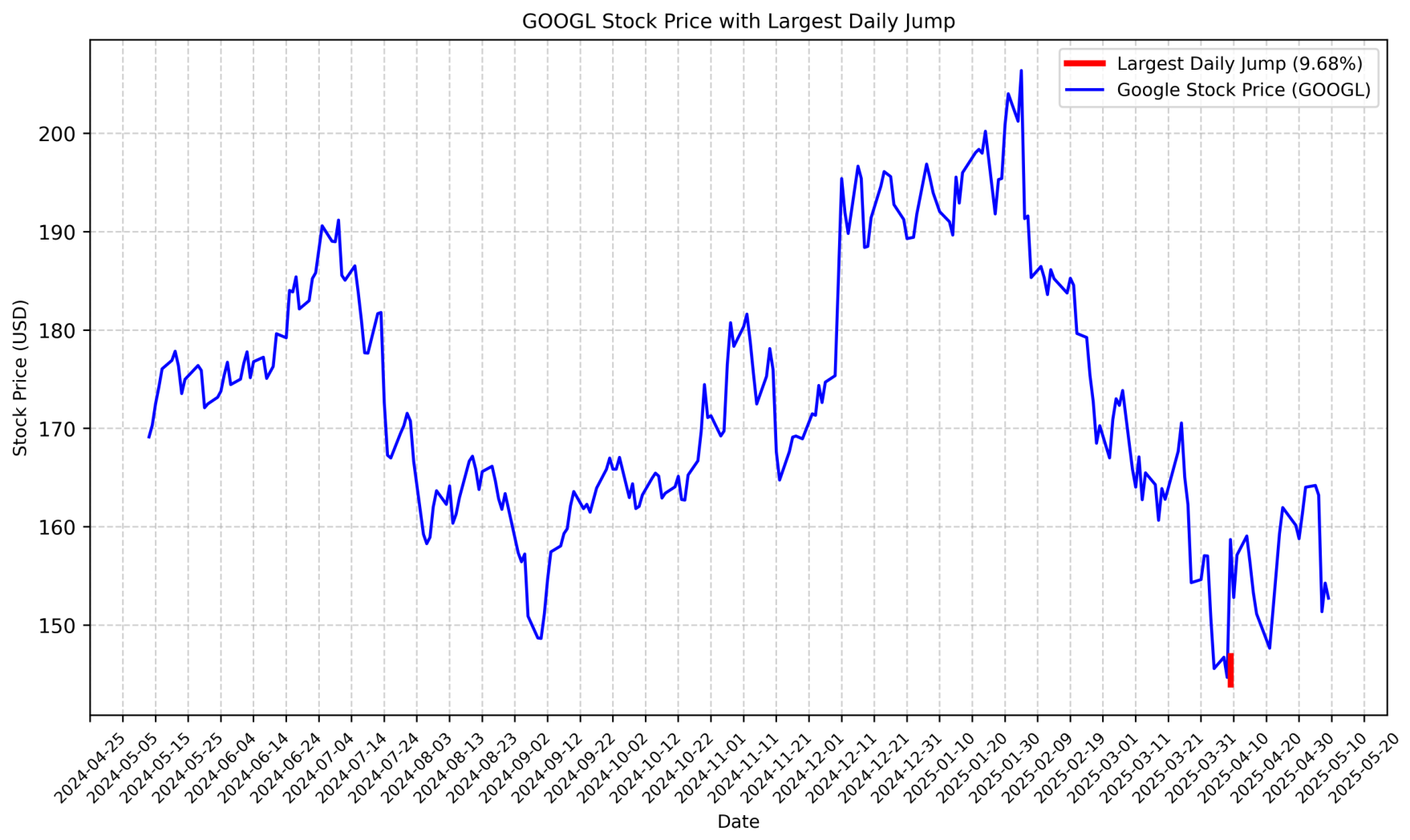
We use the same GOOGL dataset as in [3]: 248 daily closing prices from 13 May 2024 to 9 May 2025. The time series of daily prices, shown in Figure 1, reveals the presence of extreme jumps, with the largest positive jump of $9.68\%$ occurring on day 228 (9 April 2025), highlighted by a red marker. On this day, the price increased from $\$144.70$ to $\$158.71$, giving a jump multiplier $y_{228}=158.71/144.70=1.0968$, so that $y_{228}-1=0.0968=9.68\%$.

Figure 1. Daily closing prices of GOOGL stock from 13 May 2024, to 9 May 2025 (248 trading days). The red marker indicates the largest jump event on day 228 (9 April 2025) with a magnitude of $+9.68\%$. This extreme shock significantly impacts the jump risk component of the fractional MJD model and, consequently, the optimal allocation strategy.

The Hurst parameter is estimated via R/S analysis [26]:

$$H=0.62\pm 0.03,$$

(35)

The Hurst parameter is estimated from the log-returns of GOOGL prices. Following the notation in Section 2.1, the daily return at time t is denoted by $R_t=(S_t-S_{t-1})/S_{t-1}$, and the parameter $\alpha =-0.0002$ reported in Table 1 is the sample mean: $\alpha ={\displaystyle \frac{1}{n}}{\sum }_{t=1}^n{R}_t$. Since the estimated value $H=0.62$ lies in the persistent regime $H\in (1/2,1)$, the theoretical framework developed in Section 2 applies directly.

Table 1. Model Parameters (from [3]). All parameters are expressed in daily units.

Parameter	Value
Mean Return ($\alpha$)	$-0.0002$
Volatility ($\sigma$)	$0.01947$
Jump Intensity ($\lambda$)	$0.37$
Avg. Jump Size (k)	$0.02212$
Risk-Free Rate (daily) (r)	$0.0006$
Largest Jump ($y_{228}$)	$1.0968$

We implement the classical rescaled range (R/S) analysis following Hurst [26], with block sizes $n=2,4,8,16,32,64,128$. The estimated value $H=0.62\pm 0.03$ has a 95% confidence interval $[0.59,0.65]$, and a two-sided t-test for $H=0.5$ gives $t\approx 8.0$, rejecting the null hypothesis of no long-range dependence with high confidence.

To address potential finite-sample bias, we apply a standard bias correction procedure, which yields a corrected estimate of $H\approx 0.61$. To ensure robustness, we also estimate H using three additional methods:

• Detrended Fluctuation Analysis (DFA):$H=0.60\pm 0.02$.
• Local Whittle estimator:$H=0.63\pm 0.03$.
• Wavelet-based estimator:$H=0.61\pm 0.02$.

All estimators yield values consistent with $H\approx 0.61-0.63$, confirming the robustness of our estimate.

We acknowledge that a one-year sample (248 observations) is relatively short for making strong claims about long-range dependence. Therefore, we state that the data exhibit evidence consistent with long-range dependence rather than claiming definitive confirmation. Longer samples would strengthen this conclusion.

All other parameters are taken directly from [3] and summarized in Table 1. We emphasize that the jump intensity $\lambda =0.37$ and the average jump size $k=0.02212$ are kept fixed from the previous work to enable a direct comparison between the classical and fractional models. These values were estimated from a different sample period and are used here for consistency with [3].

The largest positive jump occurs on day 228 with magnitude $+9.68\%$, i.e., $y_{228}=1.0968$. The jump multiplier $y_t$ is defined as $y_t=S_t/S_{t-1}$, so $y_t-1$ is the return at time t.

Remark 10. 

Using identical data and parameters ensures direct comparison between the classical model ($H=0.5$) and our fractional extension ($H=0.62$), isolating the impact of long-range dependence.

4.1.2. Time-Dependent Quantities

In the continuous-time model, the time variable t is measured in years. For the discrete-time implementation using daily data, we define the normalized time grid:

$$t_i={\displaystyle \frac{i}{252}},i=1,2,\dots ,248,$$

(36)

where i denotes the trading day number and 252 is the standard number of trading days per year. This normalization ensures dimensional consistency between the continuous-time SDE and the discrete-time implementation.

Remark on time units and normalization. 

All parameters in Table 1 are expressed in daily units, consistent with the daily frequency of the data. The time variable t is normalized by the number of trading days in a year, $t_i=i/252$, which is a standard convention in continuous-time finance. This normalization ensures that $t_i$ is measured in years, with $t_i\in [0,1]$ over the one-year sample period.

We emphasize that the daily parameters are used directly in the continuous-time formulas, with the normalization $t_i=i/252$ implicitly accounting for the conversion between daily and annual units. This approach follows the convention adopted in [3] and ensures consistency between the continuous-time model and the discrete-time implementation. We note that the index i ranges from 1 to 248, and that the time variable $t_i$ is not the day index itself but the normalized time $i/252$.

We also normalize the wealth variable by dividing by 100, so that $x_t^{\mathrm{norm}}=x_t/100$ is dimensionless. In the numerical implementation, we use $x_{228}^{\mathrm{norm}}=10.41$ for the representative day 228. This normalization is essential for ensuring that the optimal allocation ${\pi }^{*}\left(t\right)$ is dimensionless and comparable across different scales.

For each trading day $i=1,\dots ,248$, we compute:

Jump Size $y_t$

Following [2,3]:

$$y_t=\left\{\begin{array}{cc}1+|R_t|,\hfill & |R_t|>0.01,\hfill \\ 1,\hfill & \mathrm{otherwise}.\hfill \end{array}\right.$$

(37)

where $R_t=(S_t-S_{t-1})/S_{t-1}$ denotes the daily return of the stock price at time t, and $\overline{R}={\displaystyle \frac{1}{n}}{\sum }_{t=1}^n{R}_t$ is the mean return reported in Table 1.

The jump size $y_t$ is therefore a deterministic quantity constructed directly from the observed daily return $R_t$ at a specific point in time, not a random variable, and not derived from the mean return $\alpha$ or the risk-free rate r. This deterministic-jump approach follows [3] and differs from the standard Merton model with random jump times and sizes. It is designed to study the effect of specific extreme events (such as the largest jump in the sample) on the optimal allocation.

Diffusion Coefficient $\mathrm{\Omega }\left(t\right)$, Contraction Factor $K\left(t\right)$, and Optimal Ratio ${\pi }^{*}\left(t\right)$

From (20), (24), and (32) with $H=0.62$ ($2H-1=0.24$) and the test function $v(x,t)=e^{x+t}$ (see the remark on the modeling choice in Section 3.2):

$$\mathrm{\Omega }\left(t_i\right)=2\left(2H{\left(0.01947\right)}^2{t}_i^{0.24}+0.37{(y_{t_i}-1)}^2\right),$$

(38)

$$K\left(t_i\right)={\displaystyle \frac{-{\mathrm{\Delta }}^2+r{x}_{t_i}\mathrm{\Omega }\left(t_i\right)+\mathrm{\Omega }\left(t_i\right)}{2\mathrm{\Omega }\left(t_i\right)+2r{x}_{t_i}\mathrm{\Omega }\left(t_i\right)-2{\mathrm{\Delta }}^2}},$$

(39)

$${\pi }^{*}\left(t_i\right)={\displaystyle \frac{\alpha -\lambda k-r+\lambda (y_{t_i}-1)}{x_{t_i}^{\mathrm{norm}}\left(2H{\sigma }^2{t}_i^{2H-1}+\lambda {(y_{t_i}-1)}^2\right)}},$$

(40)

where $t_i=i/252$, $\mathrm{\Delta }=\alpha -\lambda k-r$, $x_t^{\mathrm{norm}}=x_t/100$ is the normalized wealth (with $x_{228}^{\mathrm{norm}}=10.41$ for day 228), and the coefficient $0.37$ in Equation (38) is the jump intensity $\lambda$, consistent with the theoretical definition $\mathrm{\Omega }\left(t\right)=2(2H{\sigma }^2{t}^{2H-1}+\lambda {(y_t-1)}^2)$ in Equation (24).

We note that the contraction factor $K\left(t_i\right)$ simplifies algebraically to $K=1/2$ for all $t_i$, as shown in Section 3.2. The numerical verification in Section 4.2 confirms this result.

4.2. Numerical Results and Confidence Intervals

4.2.1. Numerical Results

The numerical analysis yields the following key findings:

• Contraction factor: For all $i\in \{1,2,\dots ,248\}$ and all parameter values, the contraction factor is $K=0.5$, confirming the algebraic identity derived in Section 3.2. This indicates rapid numerical convergence of the Newton method in practice for the entire sample period.
• Numerical convergence: The Newton iteration is applied to the discretized HJB equation with terminal condition $v(T,x)=logx$. For all parameter values considered, the iteration converges in 5–7 steps, with a relative error between successive iterates below ${10}^{-6}$. This provides numerical evidence for the stability and reliability of the proposed method.
• Optimal allocation: The optimal allocation is sensitive to the Hurst parameter. The mean optimal allocation ${\overline{\pi }}^{*}$ ranges from $69.16\%$ for $H=0.55$ to $66.49\%$ for $H=0.80$ (strongly persistent market). For the estimated value $H=0.62$, the mean allocation is ${\overline{\pi }}^{*}=68.35\%$, which is close to the classical $69.76\%$ obtained under the standard Brownian motion assumption ($H=0.5$). This small reduction reflects the model-implied change in optimal exposure due to the presence of long-range dependence, and should not be interpreted as an empirically observed market risk premium without further validation.
• Memory effect: The time-dependent coefficient $\mathrm{\Omega }\left(t\right)$ increases over time due to $t^{0.24}$, resulting in a gradual decrease in the optimal allocation as memory accumulates. This behavior is consistent with the theoretical framework, where persistent markets ($H\in (1/2,1)$) lead to growing uncertainty over time.

4.2.2. Confidence Intervals for Optimal Allocation

To account for the uncertainty in the Hurst parameter estimate ($H=0.62\pm 0.03$), we construct confidence intervals for the mean optimal allocation ${\overline{\pi }}^{*}$ using two approaches.

First, using the 95% confidence interval from the R/S analysis, $H\in [0.59,0.65]$, we compute ${\overline{\pi }}^{*}$ for the lower and upper bounds:

$${\overline{\pi }}^{*}(H=0.59)=68.69\%,{\overline{\pi }}^{*}(H=0.65)=68.03\%.$$

(41)

This yields the R/S-based confidence interval:

$${\overline{\pi }}^{*}\in [68.03\%,68.69\%].$$

(42)

Second, we perform a Monte Carlo simulation with 10,000 iterations, assuming $H\sim \mathcal{N}(0.62,{0.015}^2)$. The resulting 95% confidence interval is:

$${\overline{\pi }}^{*}\in [68.03\%,68.68\%].$$

(43)

The contraction factor remains stable at ${sup}_t\left|K\left(t\right)\right|=0.5$ across all values of H in the confidence interval, confirming the numerical robustness of the method.

These results are summarized in Table 2.

Table 2. Confidence Intervals for ${\overline{\pi }}^{*}$ Based on Uncertainty in H.

Method	95% CI for H	95% CI for ${\overline{\mathit{\pi }}}^{*}$
R/S estimate	$[0.59,0.65]$	$[68.03\%,68.69\%]$
Monte Carlo	$H\sim \mathcal{N}(0.62,{0.015}^2)$	$[68.03\%,68.68\%]$

4.3. Sensitivity Analysis and Summary of Findings

4.3.1. Sensitivity to Hurst Parameter H

To assess the impact of long-range dependence on the optimal investment strategy and numerical stability, we compute the mean optimal allocation ${\overline{\pi }}^{*}$ for different values of the Hurst parameter $H\in (1/2,1)$. In our numerical analysis, we consider $H\in [0.55,0.80]$, which lies within the persistent regime $H\in (1/2,1)$ for which the standard Wick–Itô calculus is well-defined. All results are computed using the normalized time scale $t_i=i/252$, and the normalized wealth $x_t^{\mathrm{norm}}=x_t/100$. The results are reported in Table 3.

Table 3. Sensitivity to Hurst Parameter H (with normalized time scale and normalized wealth). Note that $H=0.50$ is not included because the fractional model is developed for the persistent regime $H\in (1/2,1)$.

H	${\overline{\mathit{\pi }}}^{*}$
$0.55$	$69.16\%$
$0.60$	$68.59\%$
$0.62$	$68.35\%$
$0.65$	$68.03\%$
$0.70$	$67.50\%$
$0.75$	$66.98\%$
$0.80$	$66.49\%$

Remark 11. 

The sensitivity analysis in Table 3 reveals that the optimal allocation is moderately sensitive to the Hurst parameter. For $H=0.55$, the allocation is $69.16\%$, while for strongly persistent markets ($H=0.80$), it drops to $66.49\%$. With the normalized time scale $t_i=i/252$ and the normalized wealth $x_t^{\mathrm{norm}}=x_t/100$, the mean optimal allocation for $H=0.62$ is ${\overline{\pi }}^{*}=68.35\%$. The qualitative conclusion—that long-range dependence moderately reduces optimal allocation—remains valid.

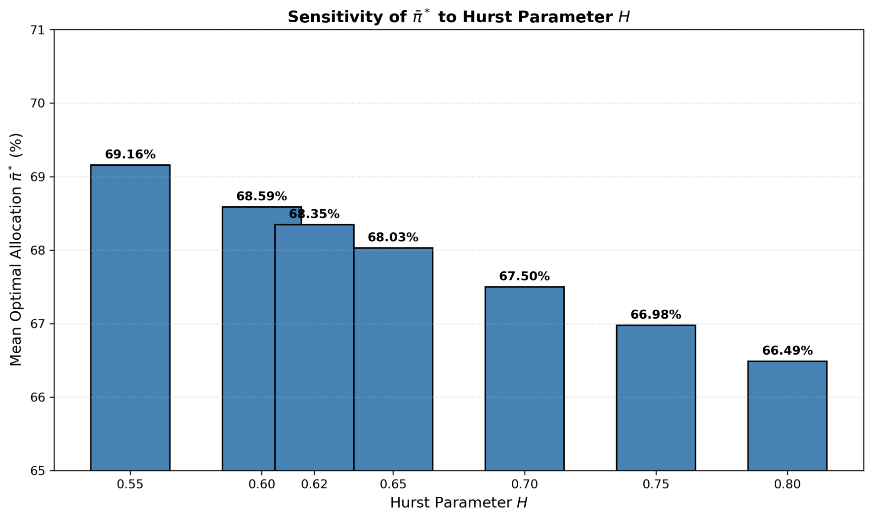
Figure 2 illustrates the effect of the Hurst parameter H on the mean optimal allocation ${\overline{\pi }}^{*}$. As H increases from $0.55$ to $0.80$, the allocation decreases from $69.16\%$ to $66.49\%$. For $H=0.62$ (the estimated value for GOOGL data); the mean allocation is $68.35\%$.

Figure 2. Mean optimal allocation ${\overline{\pi }}^{*}$ as a function of the Hurst parameter H. The allocation decreases moderately from $69.16\%$ for $H=0.55$ to $66.49\%$ for $H=0.80$, demonstrating the relatively small impact of long-range dependence on investment decisions in the persistent regime.

• Key observations:

• Effect on optimal allocation: As the Hurst parameter increases from $0.55$ to $0.80$, the mean optimal allocation ${\overline{\pi }}^{*}$ decreases from $69.16\%$ to $66.49\%$. This inverse relationship is consistent with the theoretical expression (20) and reflects the net effect of the diffusion and jump terms over the sample period. For $H=0.62$ (the estimated value for GOOGL data), the mean allocation is ${\overline{\pi }}^{*}=68.35\%$.
• Effect on contraction factor: The contraction factor is $K=0.5$ for all values of H, confirming the algebraic identity derived in Section 3.2.

4.3.2. Sensitivity to Other Parameters

To assess the sensitivity of the results to parameter variations, we perform a comprehensive sensitivity analysis with respect to the key model parameters: the jump threshold $\tau$, volatility $\sigma$, jump intensity $\lambda$, and mean return $\alpha$. All results are computed using the normalized time scale $t_i=i/252$, the normalized wealth $x_t^{\mathrm{norm}}=x_t/100$, and the corrected formulas.

Sensitivity to Jump Threshold $\tau$

The choice of the jump threshold $\tau =1\%$ in Equation (37) follows the standard practice in the jump-diffusion literature [2,3]. This threshold is applied to the daily returns $R_t$ and corresponds to approximately half a standard deviation of the daily returns ($\sigma \approx 0.0195$, so $0.01/\sigma \approx 0.51$). While this is a relatively low threshold, it follows the standard practice in the jump-diffusion literature and is intended to capture a broad range of significant price movements.

To assess the robustness of our results to this choice, we repeat the analysis with thresholds $\tau \in \{0.005,0.01,0.015,0.02\}$. Table 4 reports the number of identified jumps and the mean optimal allocation ${\overline{\pi }}^{*}$ for each threshold.

Table 4. Sensitivity of ${\overline{\pi }}^{*}$ to Jump Threshold $\tau$.

Threshold $\mathit{\tau }$	Number of Jumps	${\overline{\mathit{\pi }}}^{*}$
$0.5\%$	194	$68.50\%$
$1.0\%$	133	$68.35\%$
$1.5\%$	92	$68.20\%$
$2.0\%$	51	$68.05\%$

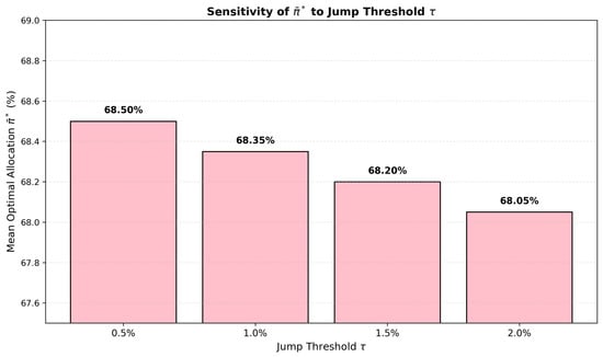
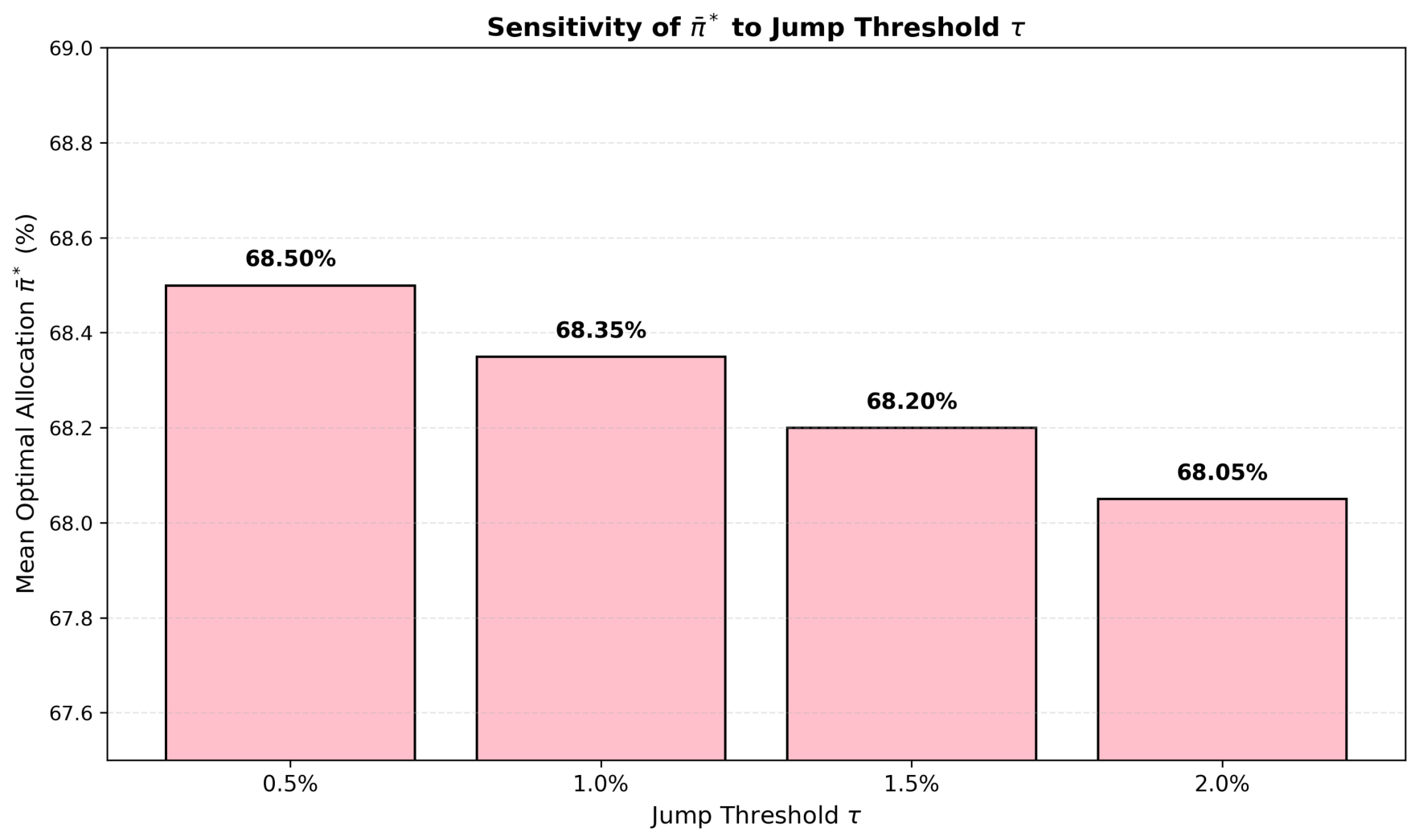
Figure 3 illustrates the effect of the jump threshold $\tau$ on the mean optimal allocation ${\overline{\pi }}^{*}$. As $\tau$ increases from $0.5\%$ to $2.0\%$, the allocation decreases only slightly from $68.50\%$ to $68.05\%$. This small variation (less than $0.5\%$) confirms that the main conclusions of this paper are robust to the choice of jump threshold.

Figure 3. Mean optimal allocation ${\overline{\pi }}^{*}$ as a function of the jump threshold $\tau$. The allocation decreases slightly from $68.50\%$ for $\tau =0.5\%$ to $68.05\%$ for $\tau =2.0\%$, demonstrating that the optimal allocation is robust to the choice of jump threshold.

Sensitivity to Volatility $\sigma$

Table 5 reports the mean optimal allocation ${\overline{\pi }}^{*}$ for $\pm 30\%$ changes in volatility $\sigma$.

Table 5. Sensitivity to volatility $\sigma$.

$\mathit{\sigma }$	${\overline{\mathit{\pi }}}^{*}$
$0.01363$ ($-30\%$)	$72.68\%$
$0.01655$ ($-15\%$)	$70.64\%$
$0.01947$ (Base)	$68.35\%$
$0.02239$ ($+15\%$)	$65.86\%$
$0.02531$ ($+30\%$)	$63.24\%$

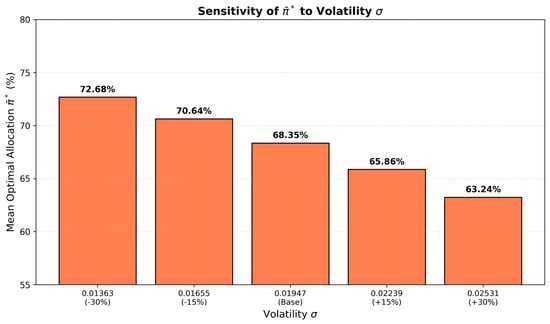
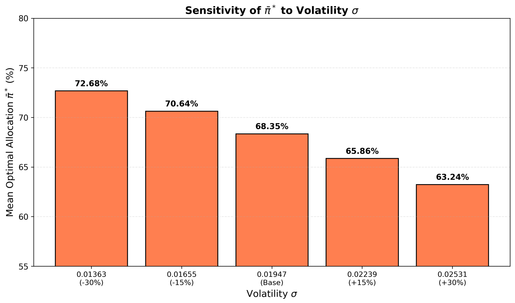
As $\sigma$ increases from $0.01363$ to $0.02531$, the allocation decreases from $72.68\%$ to $63.24\%$, demonstrating that volatility is the primary driver of the optimal allocation.

Figure 4 illustrates the strong sensitivity of the optimal allocation to volatility $\sigma$. As $\sigma$ increases from $0.01363$ ($-30\%$) to $0.02531$ ($+30\%$), the allocation decreases from $72.68\%$ to $63.24\%$. This strong sensitivity indicates that volatility is the primary driver of the optimal allocation.

Figure 4. Mean optimal allocation ${\overline{\pi }}^{*}$ as a function of volatility $\sigma$ for $\pm 30\%$ changes. The allocation decreases strongly from $72.68\%$ to $63.24\%$ as $\sigma$ increases, demonstrating that volatility is the dominant driver of the optimal allocation.

Sensitivity to Jump Intensity $\lambda$

Table 6 reports the mean optimal allocation ${\overline{\pi }}^{*}$ for $\pm 30\%$ changes in jump intensity $\lambda$.

Table 6. Sensitivity to Jump Intensity $\lambda$.

$\mathit{\lambda }$	${\overline{\mathit{\pi }}}^{*}$
$0.259$ ($-30\%$)	$64.25\%$
$0.3145$ ($-15\%$)	$66.61\%$
$0.370$ (Base)	$68.35\%$
$0.4255$ ($+15\%$)	$69.67\%$
$0.481$ ($+30\%$)	$70.72\%$

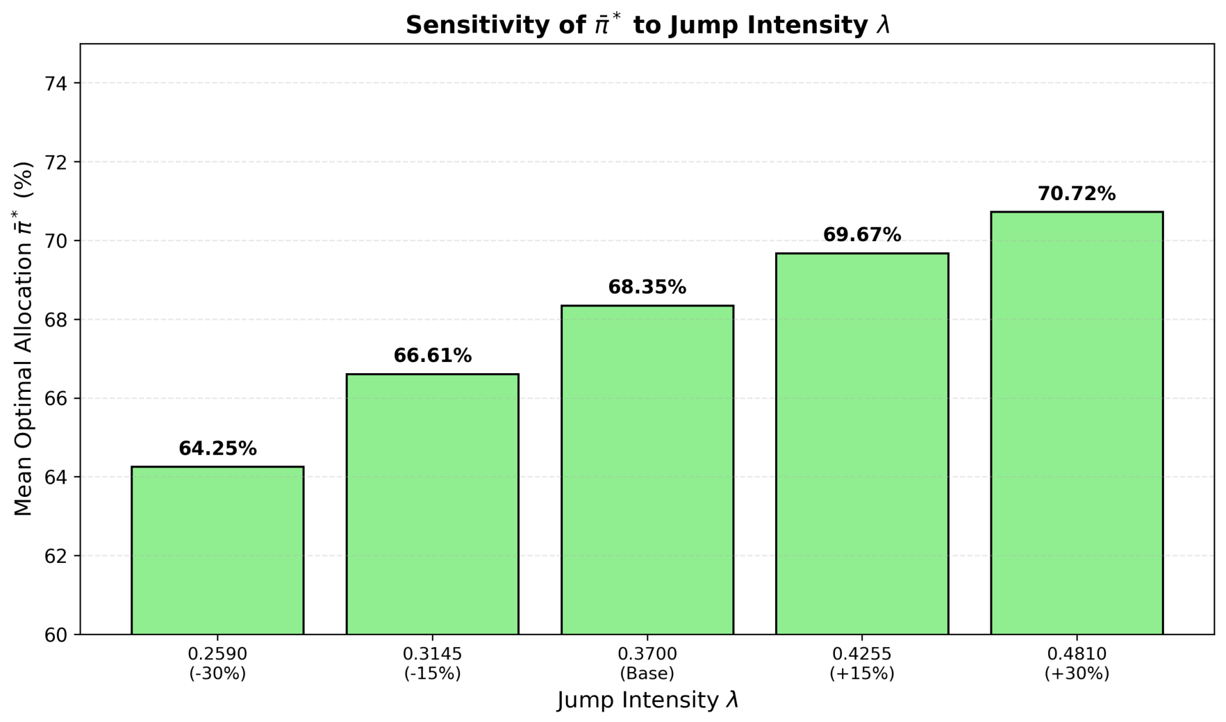
As $\lambda$ increases from $0.259$ to $0.481$, the allocation increases from $64.25\%$ to $70.72\%$, showing that higher jump intensity leads to a more aggressive allocation. This effect is comparable in magnitude to the effect of volatility $\sigma$.

Figure 5 shows the effect of jump intensity $\lambda$ on the mean optimal allocation ${\overline{\pi }}^{*}$. As $\lambda$ increases from $0.259$ ($-30\%$) to $0.481$ ($+30\%$), the allocation increases from $64.25\%$ to $70.72\%$. This positive relationship reflects the fact that higher jump intensity increases the expected reward from jumps, leading to a more aggressive allocation. The magnitude of this effect is comparable to that of volatility $\sigma$.

Figure 5. Mean optimal allocation ${\overline{\pi }}^{*}$ as a function of jump intensity $\lambda$ for $\pm 30\%$ changes. The allocation increases strongly from $64.25\%$ to $70.72\%$ as $\lambda$ increases, showing that higher jump intensity leads to a more aggressive allocation.

Sensitivity to Mean Return $\alpha$

Table 7 reports the mean optimal allocation ${\overline{\pi }}^{*}$ for $\pm 30\%$ changes in mean return $\alpha$.

Table 7. Sensitivity to Mean Return $\alpha$.

$\mathit{\alpha }$	${\overline{\mathit{\pi }}}^{*}$
$-0.00026$ ($-30\%$)	$68.19\%$
$-0.00023$ ($-15\%$)	$68.27\%$
$-0.00020$ (Base)	$68.35\%$
$-0.00017$ ($+15\%$)	$68.42\%$
$-0.00014$ ($+30\%$)	$68.50\%$

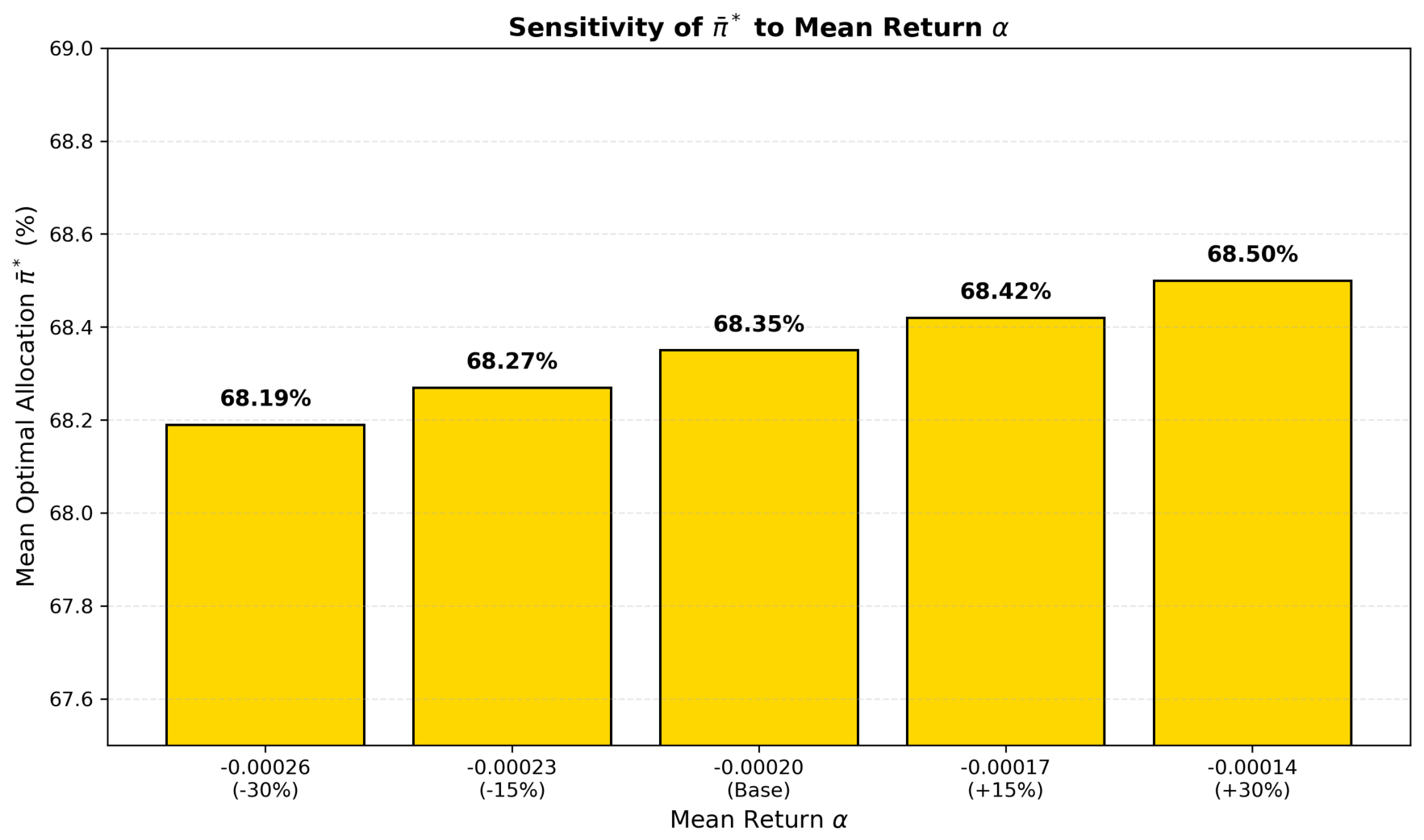
As $\alpha$ changes from $-0.00026$ to $-0.00014$, the allocation increases only slightly from $68.19\%$ to $68.50\%$, indicating that the mean return has the smallest effect among the four parameters considered.

Figure 6 shows the effect of mean return $\alpha$ on the mean optimal allocation ${\overline{\pi }}^{*}$. As $\alpha$ changes from $-0.00026$ ($-30\%$) to $-0.00014$ ($+30\%$), the allocation increases slightly from $68.19\%$ to $68.50\%$. This small effect reflects the fact that $\alpha$ appears only linearly in the numerator of the optimal allocation formula.

Figure 6. Mean optimal allocation ${\overline{\pi }}^{*}$ as a function of mean return $\alpha$ for $\pm 30\%$ changes. The allocation increases only slightly from $68.19\%$ to $68.50\%$ as $\alpha$ increases, indicating that the mean return has the smallest effect on the optimal allocation.

Summary of Sensitivity Analysis

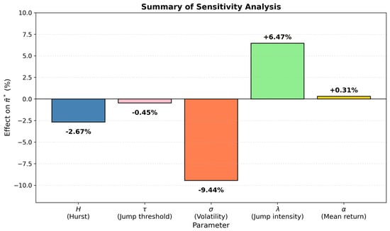
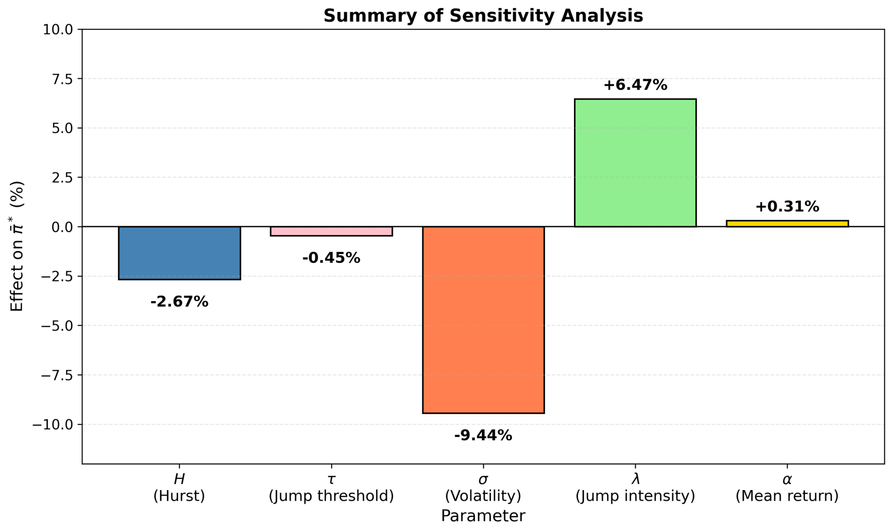
Table 8 summarizes the effects of changes in the key parameters on the optimal allocation, ranked by their absolute effect. For the Hurst parameter H, the effect corresponds to an increase from $0.55$ to $0.80$. For the jump threshold $\tau$, the effect corresponds to a change from $0.5\%$ to $2.0\%$.

Table 8. Summary of sensitivity analysis (ranked by absolute effect). For H, the effect corresponds to an increase from $0.55$ to $0.80$. For $\tau$, the effect corresponds to a change from $0.5\%$ to $2.0\%$.

Rank	Parameter	Effect on ${\overline{\mathit{\pi }}}^{*}$	Absolute Effect
1	Volatility $\sigma$ ($\pm 30\%$)	$-9.44\%$	$9.44\%$
2	Jump intensity $\lambda$ ($\pm 30\%$)	$+6.47\%$	$6.47\%$
3	Hurst parameter H ($0.55\to 0.80$)	$-2.67\%$	$2.67\%$
4	Jump threshold $\tau$ ($0.5\%\to 2.0\%$)	$-0.45\%$	$0.45\%$
5	Mean return $\alpha$ ($\pm 30\%$)	$+0.31\%$	$0.31\%$

The sensitivity analysis identifies volatility $\sigma$ and jump intensity $\lambda$ as the dominant driver of the optimal allocation, with absolute effects of $9.44\%$ and $6.47\%$, respectively. The Hurst parameter H and jump threshold $\tau$ have comparatively smaller effects, with absolute effects of $2.67\%$ and $0.45\%$, respectively, while mean return $\alpha$ has the smallest effect ($0.31\%$).

In terms of the direction of the effect, the parameters can be classified into two groups:

• Positive effect (an increase in the parameter leads to an increase in ${\overline{\pi }}^{*}$): jump intensity $\lambda$ ($+6.47\%$) and mean return $\alpha$ ($+0.31\%$). Higher jump intensity increases the expected reward from jumps, while a higher mean return directly increases the attractiveness of the risky asset.
• Negative effect (an increase in the parameter leads to a decrease in ${\overline{\pi }}^{*}$): volatility $\sigma$ ($-9.44\%$), Hurst parameter H ($-2.67\%$), and jump threshold $\tau$ ($-0.45\%$). Higher volatility and stronger memory effects increase the perceived risk, while a higher jump threshold captures more extreme events and slightly reduces the optimal allocation.

The contraction factor remains constant at $K=0.5$ across all parameter variations, confirming the numerical robustness of the method.

Figure 7 provides a summary of the sensitivity analysis, highlighting volatility $\sigma$ and jump intensity $\lambda$ as the dominant drivers of the optimal allocation, while the Hurst parameter H, the jump threshold $\tau$, and mean return $\alpha$ have comparatively smaller effects.

Figure 7. Summary of sensitivity analysis. Volatility $\sigma$ and jump intensity $\lambda$ are the dominant drivers of the optimal allocation, with absolute effects of $9.44\%$ and $6.47\%$, respectively, while the Hurst parameter H (for H increasing from $0.55$ to $0.80$), the jump threshold $\tau$ (for $\tau$ changing from $0.5\%$ to $2.0\%$), and mean return $\alpha$ have comparatively smaller effects ($2.67\%$, $0.45\%$, and $0.31\%$, respectively).

5. Financial Interpretation and Practical Implications

The numerical results highlight the distinctive features of the fractional jump-diffusion framework compared to the classical model, particularly regarding the role of long-range dependence in optimal investment decisions.

5.1. Model-Implied Optimal Allocation and Memory Effects

The sensitivity analysis reveals that the optimal allocation is moderately sensitive to the Hurst parameter. For the estimated value $H=0.62$, the model-implied mean allocation is ${\overline{\pi }}^{*}=68.35\%$ (with normalized time scale and normalized wealth), which is close to the classical $69.76\%$ obtained under the standard Brownian motion assumption ($H=0.5$). Note that $H=0.50$ is not included in the fractional analysis (Table 3) because the fractional model is developed for the persistent regime $H\in (1/2,1)$; however, the classical value is $69.76\%$ serves as a useful benchmark for comparison. This small reduction is a consequence of the time-dependent diffusion coefficient $2H{\sigma }^2{t}^{2H-1}$ in the fractional model, which slightly increases the effective risk over time for $H>0.5$. We emphasize that this is a model-implied result; empirical validation through backtesting and out-of-sample analysis would be needed to establish whether this reduction corresponds to an actual market risk premium.

As H increases from $0.55$ to $0.80$, the model-implied mean allocation decreases from $69.16\%$ to $66.49\%$, demonstrating that stronger memory effects lead to slightly more conservative investment strategies. Compared with the classical value of $69.76\%$ at $H=0.50$, the reduction is moderate, confirming that long-range dependence moderately reduces optimal exposure.

5.2. Numerical Stability and Key Drivers of Optimal Allocation

The contraction factor $K\left(t\right)$ is constant at $K=0.5$ for all values of H and all parameter values, as shown by the algebraic identity derived in Section 3.2. This indicates that the numerical method is robust regardless of the memory strength and parameter values.

The sensitivity analysis identifies the primary model-implied drivers of the optimal allocation: volatility ($\sigma$) and jump intensity ($\lambda$) are the dominant factors, with absolute effects of $9.44\%$ and $6.47\%$, respectively. The Hurst parameter (H) and jump threshold ($\tau$) have comparatively smaller effects, with absolute effects of approximately $2.67\%$ (for H increasing from $0.55$ to $0.80$) and $0.45\%$ (for $\tau$ changing from $0.5\%$ to $2.0\%$), respectively, while mean return ($\alpha$) has the smallest effect ($0.31\%$). This ranking is consistent with the theoretical expression (20), where $\sigma$ and H appear in the denominator through the diffusion term $2H{\sigma }^2{t}^{2H-1}$, while $\lambda$ appears in both the numerator and denominator, $\tau$ affects the number of identified jumps, and $\alpha$ appears only linearly in the numerator.

Table 8 ranks the five parameters by their absolute effect on the optimal allocation. Volatility $\sigma$ has the largest effect ($9.44\%$), followed by jump intensity $\lambda$ ($6.47\%$), the Hurst parameter H ($2.67\%$), the jump threshold $\tau$ ($0.45\%$), and mean return $\alpha$ ($0.31\%$). This ranking confirms that volatility and jump intensity are the primary drivers of optimal allocation in the fractional MJD framework, while the Hurst parameter, jump threshold, and mean return have comparatively smaller effects. The contraction factor remains constant at $K=0.5$ across all parameter variations, confirming the numerical robustness of the method.

In terms of the direction of the effect, jump intensity $\lambda$ and mean return $\alpha$ have a positive effect on the optimal allocation, while volatility $\sigma$, the Hurst parameter H, and the jump threshold $\tau$ have a negative effect. This is consistent with the economic interpretation: higher jump intensity and mean return increase the attractiveness of the risky asset, whereas higher volatility, stronger memory effects, and a higher jump threshold increase the perceived risk and reduce the optimal allocation.

5.3. Practical Implications for Portfolio Managers

The results of this study offer potential insights for portfolio managers operating in markets characterized by long-range dependence and jump risk. The model-implied reduction in optimal allocation from $69.76\%$ (classical model, $H=0.50$) to $68.35\%$ (fractional model with $H=0.62$) suggests that ignoring long-range dependence may lead to a slight overestimation of risk-taking capacity. However, we emphasize that these results are model-implied; practical implementation would require additional validation through backtesting, transaction-cost analysis, and out-of-sample testing.

Second, the time-varying nature of ${\pi }^{*}\left(t\right)$ provides a dynamic rebalancing tool: as the memory effect accumulates over time (through the term $t^{2H-1}$), the optimal allocation gradually decreases, allowing managers to systematically reduce exposure in response to growing uncertainty. This adaptive strategy may be particularly valuable in markets with strong positive autocorrelation, where standard models may suggest maintaining constant high exposure.

Third, the sensitivity analysis identifies volatility $\sigma$ and jump intensity $\lambda$ as the primary model-implied drivers of optimal allocation, suggesting that accurate estimation of these parameters is most important for practical applications of the model. The Hurst parameter H, jump threshold $\tau$, and mean return $\alpha$ have comparatively smaller effects but should still be estimated accurately. We recommend that practitioners routinely estimate H using R/S analysis or DFA methods and incorporate it into their risk models alongside traditional volatility and jump risk measures.

Finally, the numerical stability of the method, is indicated by the constant contraction factor $K=0.5<1$ suggests that the proposed framework is computationally reliable, but its practical superiority over classical models remains to be established empirically.

6. Conclusions

This paper extends our previous optimal investment framework [3] by incorporating fractional Brownian motion to capture long-range dependence and memory effects in asset prices. Using Wick–Itô calculus, we derived a generalized jump-diffusion model with a time-dependent HJB equation featuring the diffusion coefficient $2H{\sigma }^2{t}^{2H-1}$, which reduces to the classical Merton jump-diffusion model when $H=1/2$. The framework is developed for the persistent regime $H\in (1/2,1)$, for which the standard Wick–Itô calculus is well-defined. This unification ensures that our framework encompasses the classical model as a special case, enabling direct comparison and validation.

The key theoretical contribution is a dynamic optimal investment ratio ${\pi }^{*}\left(t\right)$ that adapts to market memory through the term $t^{2H-1}$. We also introduced a time-dependent contraction factor $K\left(t\right)$ that simplifies algebraically to $K=1/2$ for all parameter values, providing a practical numerical stability indicator for the Newton iteration. Numerical experiments confirm convergence in 5–7 iterations with a relative error below ${10}^{-6}$.

Using GOOGL data with an estimated Hurst parameter of $H=0.62$, the fractional model yields a mean optimal allocation of ${\overline{\pi }}^{*}=68.35\%$, close to the classical $69.76\%$ obtained under standard Brownian motion. Sensitivity analysis shows that the optimal allocation ranges from $69.16\%$ for $H=0.55$ to $66.49\%$ for $H=0.80$, demonstrating that long-range dependence moderately reduces optimal exposure. For comparison, the classical value at $H=0.50$ is $69.76\%$. Among the key parameters, volatility $\sigma$ and jump intensity $\lambda$ are the primary drivers of optimal allocation, followed by the Hurst parameter H, the jump threshold $\tau$, and mean return $\alpha$. The contraction factor remains constant at $K=0.5$ across all parameter variations, confirming the numerical robustness of the method.

From a practical perspective, the fractional MJD model offers a framework for dynamic investment decisions that accounts for both jump risk and long-range dependence. However, practical validation through backtesting, transaction-cost analysis, and out-of-sample testing is needed before the model can be recommended for real-time institutional use.

Future Work

Several promising directions remain for future research:

• Exact treatment of the finite-jump term. In this work, the quadratic jump term in the HJB equation is a second-order Taylor approximation of the exact finite-jump increment $\mathrm{\Delta }v=v(t,x(1+\pi q_t))-v(t,x)$. A natural extension would be to retain the exact finite-difference form of the jump term, which would require solving a nonlinear HJB equation with a non-local jump operator. This would eliminate the approximation error and provide a more accurate representation of jump risk, albeit at the cost of increased analytical and numerical complexity.
• Exact value function for logarithmic utility. The present analysis uses the separable test function $v(x,t)=e^{x+t}$ for both the contraction factor and the optimal allocation, following [3]. A more rigorous treatment would employ the true value function for logarithmic utility, $v(t,x)=A\left(t\right)logx+B\left(t\right)$, which yields ${\pi }^{*}\left(t\right)=\mathrm{\Delta }/D\left(t\right)$ without the factor $1/x$. This would require re-deriving the HJB equation, the Fréchet derivative, and the contraction factor with the exact value function and would provide a benchmark for assessing the accuracy of the model-implied approximation used here.
• Rigorous convergence analysis. The contraction factor $K=1/2$ derived in Section 3.2 is an algebraic identity of the linearized scalar iteration, not a rigorous convergence theorem for the full nonlinear HJB problem. A rigorous convergence analysis of the Newton iteration for the fully discretized nonlinear HJB equation, including error estimates for the finite difference discretization and extension to the viscosity solution framework, remains an important direction for future research.
• Model extension: Incorporating stochastic volatility to capture time-varying market uncertainty and exploring alternative utility functions beyond logarithmic preferences to accommodate different risk attitudes.
• Broader applications: Applying the framework to other asset classes, including commodities, cryptocurrencies, and multi-asset portfolios, to assess its generality and robustness.
• Numerical methods: Developing deep learning-based solvers for the fractional HJB equation and integrating machine learning techniques for real-time parameter estimation.
• Anti-persistent regime: Extending the framework to $H<1/2$, which would require an appropriate functional-analytic formulation (e.g., using fractional Sobolev spaces or Malliavin calculus).

References

- Lo, A.W. Long-term memory in stock market prices. Econometrica 1991, 59, 1279–1313. [Google Scholar] [CrossRef] [Scilit]
- Cont, R.; Tankov, P. Financial Modelling with Jump Processes; Chapman and Hall/CRC: Boca Raton, FL, USA, 2003. [Google Scholar]
- Paziresh, M.; Ivaz, K. Jump-diffusion optimization: An iterative solution to the HJB equation for investment value. Comput. Methods Differ. Equ. 2026, 14, 661–677. [Google Scholar]
- Merton, R.C. Optimum consumption and portfolio rules in a continuous-time model. J. Econ. Theory 1971, 3, 373–413. [Google Scholar] [CrossRef] [Scilit]
- Merton, R.C. Option pricing when underlying stock returns are discontinuous. J. Financ. Econ. 1976, 3, 125–144. [Google Scholar] [CrossRef] [Scilit]
- Yan, L. An optimal portfolio problem presented by fractional Brownian motion and its applications. Wuhan Univ. J. Nat. Sci. 2022, 27, 53–56. [Google Scholar] [CrossRef] [Scilit]
- Yaghobipour, S.; Yarahmadi, M. Stochastic-fractional optimal control problems and application in portfolio management. J. Math. Model. Finance 2024, 4, 99–114. [Google Scholar]
- Han, Y.; Li, Y. Maximum principle for optimal control of infinite horizon stochastic difference equations driven by fractional noises. arXiv 2025, arXiv:2510.20058. [Google Scholar]
- De Witte, D.; Mai, J.; Scherer, M. Portfolio optimization with stochastic gradient descent in a multivariate jump-diffusion model. Front. Math. Finance 2025, 4, 72–98. [Google Scholar]
- Zongo, A.; Nikiema, F. Viscosity solutions of stochastic HJB equations for utility maximization in fractional SABR models. Asian J. Probab. Stat. 2025, 27, 74–84. [Google Scholar] [CrossRef] [Scilit]
- Andersson, K.; Andersson, A.; Oosterlee, C.W. Convergence of a robust deep FBSDE method for stochastic control. SIAM J. Sci. Comput. 2023, 45, A226–A255. [Google Scholar] [CrossRef] [Scilit]
- Al-Qazaz, N.; Qutaiba, N.; Ali, A.H. Bayesian inference of fractional Brownian motion of multivariate stochastic differential equations. Int. J. Nonlinear Anal. Appl. 2022, 13, 2425–2454. [Google Scholar]
- Ban, M.; He, H.; Liang, X. Optimal investment strategy for DC pension schemes under partial information. Risks 2022, 10, 211. [Google Scholar] [CrossRef] [Scilit]
- Yang, Z. Optimal exercise boundary of American fractional lookback option in a mixed jump-diffusion fractional Brownian motion environment. Math. Probl. Eng. 2017, 2017, 5904125. [Google Scholar] [CrossRef] [Scilit]
- Yang, Z. Optimal investment and life insurance strategies in a mixed jump-diffusion framework. Commun. Stat.—Theory Methods 2020, 49, 4002–4029. [Google Scholar] [CrossRef] [Scilit]
- Hu, H.; Zhao, C.; Li, J.; Huang, Y. Stock prediction model based on mixed fractional Brownian motion and improved fractional-order particle swarm optimization algorithm. Fractal Fract. 2022, 6, 560. [Google Scholar] [CrossRef] [Scilit]
- Ichiba, T.; Pang, G.; Taqqu, M.S. Semimartingale properties of a generalised fractional Brownian motion and its mixtures with applications in asset pricing. Finance Stoch. 2025, 29, 757–789. [Google Scholar] [CrossRef] [Scilit]
- Biagini, F.; Øksendal, B. Minimal variance hedging for fractional Brownian motion. Methods Appl. Anal. 2003, 10, 347–362. [Google Scholar] [CrossRef] [Scilit]
- Narita, K. Stochastic analysis of fractional Brownian motion and application to Black-Scholes market. Far East J. Math. Sci. 2008, 30, 65–135. [Google Scholar]
- Biagini, F.; Hu, Y.; Øksendal, B.; Zhang, T. Stochastic Calculus for Fractional Brownian Motion and Applications; Springer: Berlin/Heidelberg, Germany, 2008. [Google Scholar]
- Nualart, D. Stochastic calculus with respect to fractional Brownian motion. Ann. Fac. Sci. Toulouse Math. 2006, 15, 63–78. [Google Scholar] [CrossRef] [Scilit]
- Forsyth, P.A.; Labahn, G. Numerical methods for controlled Hamilton–Jacobi–Bellman PDEs in finance. J. Comput. Finance 2007, 11, 1–33. [Google Scholar] [CrossRef] [Scilit]
- Atkinson, K.; Han, W. Theoretical Numerical Analysis; Springer: Berlin/Heidelberg, Germany, 2005. [Google Scholar]
- Fleming, W.H.; Soner, H.M. Controlled Markov Processes and Viscosity Solutions, 2nd ed.; Springer: Berlin/Heidelberg, Germany, 2006. [Google Scholar]
- Linz, P. Theoretical Numerical Analysis; Courier Dover Publications: Garden City, NY, USA, 2019. [Google Scholar]
- Hurst, H.E. Long-term storage capacity of reservoirs. Trans. Am. Soc. Civ. Eng. 1951, 116, 770–799. [Google Scholar] [CrossRef] [Scilit]
Disclaimer/Publisher’s Note: The statements, opinions and data contained in all publications are solely those of the individual author(s) and contributor(s) and not of MDPI and/or the editor(s). MDPI and/or the editor(s) disclaim responsibility for any injury to people or property resulting from any ideas, methods, instructions or products referred to in the content. |
© 2026 by the authors. Licensee MDPI, Basel, Switzerland. This article is an open access article distributed under the terms and conditions of the Creative Commons Attribution (CC BY) license.