Fairness-Aware Opinion Seeding in Undirected Signed Friedkin–Johnsen Networks

Abstract

Opinion-maximization methods often optimize an aggregate network response and may therefore distribute target-aligned intervention gains unevenly across groups. This issue is especially important in signed networks, where cooperative and antagonistic relations can make the same positive opinion seed increase the equilibrium opinion of one group while decreasing that of another. We study fairness-aware internal-opinion seeding in undirected signed Friedkin–Johnsen networks with heterogeneous anchoring strengths. The objective combines the whole-network average opinion gain with the minimum group-average gain through a tunable fairness parameter. We show that the equilibrium response of any seed set decomposes additively into candidate-wise group-gain vectors. This representation yields an equivalent mixed-integer linear program for exact optimization on tractable instances and an adjoint formulation that evaluates all candidate gains using only one shifted signed-Laplacian solve per group. Because the global averaging vector is a size-weighted combination of the group averaging vectors, no additional global solve is required. We further introduce a dynamically maintained Pareto frontier based on componentwise dominance and establish conditions under which pruning preserves the underlying greedy sequence. Theoretical results establish well-posedness and stability of the signed equilibrium, correctness of the gain and adjoint formulations, sufficient conditions for monotonicity, non-submodularity in general, residual-based numerical error bounds, and computational complexity. Experiments on 14 signed networks ranging from hundreds to more than four million nodes show that the adjoint implementation scales most robustly among the tested methods. The results further demonstrate that the fairness parameter and heterogeneous anchoring strengths can substantially affect both the selected seed sets and the fairness–efficiency balance. Against structural, random, and target-aware Top-K baselines, the proposed greedy method remains broadly competitive, and on small full-candidate instances it matches the solver-certified mixed-integer linear program (MILP) optimum in five of six tested configurations. Overall, the framework provides a scalable approach to group-aware opinion intervention in signed networks while explicitly distinguishing opinion seeding from clamped leader selection.

1. Introduction

Signed networks represent relationships of opposite polarity, including trust and distrust, agreement and opposition, and cooperation and antagonism. Unlike unsigned networks, the sign of an interaction is not merely an auxiliary label: positive edges tend to promote alignment, whereas negative edges favor disagreement or sign reversal. As a result, ignoring edge signs can alter both the magnitude and the direction of an intervention response [1,2,3,4].

The DeGroot and Friedkin–Johnsen models are classical mathematical models of opinion evolution [5,6,7]. The Friedkin–Johnsen model is well suited to intervention analysis because it combines interpersonal influence with persistent internal opinions and has a linear equilibrium representation. This structure has supported a variety of optimization problems involving internal-opinion modification, external sources, stubbornness or anchoring parameters, clamped leaders, link recommendation, and polarization or disagreement reduction [8,9,10,11,12,13,14]. Most existing formulations, however, optimize a single aggregate quantity over the entire network. A large aggregate gain does not imply that every subgroup benefits from an intervention, and this mismatch can be particularly pronounced in signed networks because positive and negative paths may produce opposite responses across different groups.

Fairness considerations have therefore become important in network intervention problems. Fair influence maximization has studied group coverage, welfare aggregation, demographic-parity criteria, and distribution-sensitive objectives in stochastic diffusion models [15,16,17,18,19,20]. More recent work has considered fairness directly in opinion propagation and Friedkin–Johnsen dynamics [21,22,23]. Nevertheless, fairness-aware opinion intervention in signed Friedkin–Johnsen systems remains less understood. In particular, antagonistic edges may cause the same internal-opinion intervention to help one group while harming another, which makes aggregate opinion maximization insufficient for controlling group-level outcomes.

In this paper, we study fairness-aware internal-opinion seeding in an undirected weighted signed Friedkin–Johnsen network. Each node has an internal opinion and an anchoring strength that may vary across nodes. A prescribed partition divides the network into groups, and a candidate set specifies which nodes are eligible for intervention. Selecting a positive opinion seed changes its internal opinion to the positive extreme but does not clamp its expressed opinion. The selected node continues to evolve according to the Friedkin–Johnsen equilibrium. We measure the resulting change in equilibrium opinion both globally and separately for each group, and optimize a convex combination of the whole-network average gain and the worst-group average gain. The group memberships are fixed at baseline. When external group labels are unavailable, signed-degree-based opinion strata provide a reproducible way to study distributional effects. These strata should not be interpreted as demographic groups.

The resulting optimization problem has a useful linear form. Because the Friedkin–Johnsen equilibrium is linear in the internal-opinion vector, the contribution of each selected seed to each group can be represented by a candidate-specific group-gain vector. This converts the original network intervention problem into a multidimensional discrete selection problem over precomputed gain vectors. The representation yields an exact mixed-integer linear formulation for tractable candidate sets. At the same time, direct column-wise recovery of the response matrix is computationally expensive on large networks. We therefore derive an adjoint formulation that evaluates all candidate gains using only one shifted signed-Laplacian solve per group, rather than one solve per candidate or per network node. Since the global average is a size-weighted combination of the group averages, no separate global solve is needed.

The group-gain representation also reveals why the fairness objective is combinatorially difficult. Each individual group gain is modular, but taking the minimum across groups introduces complementarity between candidates. Consequently, the complete objective is not submodular in general, and classical monotone-submodular approximation guarantees do not directly apply. To reduce candidate scoring while preserving the greedy rule, we use componentwise Pareto dominance and maintain a dynamic frontier of nondominated candidates. We further distinguish numerical gain-computation error from the structural gap between greedy selection and exact mixed-integer optimization.

The main contributions of this work are summarized as follows.

• We formulate fairness-aware internal-opinion seeding in undirected signed Friedkin–Johnsen networks with heterogeneous anchoring strengths. The objective balances the whole-network average equilibrium gain and the minimum group-average gain while explicitly separating the propagation model, baseline-fixed group partition, candidate set, and intervention budget.
• We derive an additive candidate-wise group-gain decomposition. Each candidate is represented by an r-dimensional group-gain vector, and the global gain is shown to be a size-weighted combination of the group gains. This representation yields an equivalent mixed-integer linear program for exact optimization on tractable instances.
• We develop an adjoint gain-computation method that obtains the gains of all candidates using only r shifted signed-Laplacian solves. A column-solve formulation is retained as a reference implementation, while the adjoint formulation avoids constructing the dense response matrix and is suitable for large signed networks.
• We introduce a dynamically maintained Pareto frontier based on componentwise dominance. Under the prescribed tie rule and exact or certified dominance comparisons, pruning preserves the underlying greedy sequence.
• We establish theoretical properties of the framework, including existence and stability of the signed Friedkin–Johnsen equilibrium, correctness of the gain and adjoint formulations, sufficient conditions for monotonicity, non-submodularity in general, residual-based numerical error bounds, and computational complexity. We also use a best-prefix strategy for the at-most-k variant. This strategy allows the algorithm to continue through nonimproving intermediate steps and identify complementary seed sets.
• We provide an empirical evaluation on 14 signed networks ranging from hundreds to more than four million nodes. The experiments examine scalability; the effect of the fairness parameter; heterogeneous anchoring strengths; comparisons with structural, random, and target-aware baselines; and MILP-certified optimality gaps. The adjoint implementation scales most robustly among the tested methods, and the scalable greedy methods match the solver-certified MILP optimum in five of six small full-candidate configurations.

The remainder of the paper is organized as follows. Section 2 reviews related work. Section 3 introduces the signed Friedkin–Johnsen model, the shifted signed-Laplacian solver, and the group construction. Section 4 defines the fairness-aware opinion-seeding problem. Section 5 derives the candidate-gain representation and the exact mixed-integer formulation. Section 6 presents the greedy and pruning algorithms. Section 7 provides the theoretical, numerical, and complexity analysis. Section 8 reports the experimental evaluation. Section 9 discusses extensions, interpretation, and limitations, and Section 10 concludes the paper.

2. Related Work

2.1. Friedkin–Johnsen Interventions

DeGroot averaging models describe repeated social learning, whereas the Friedkin–Johnsen model retains internal opinions and heterogeneous resistance to interpersonal influence [5,6,7]. Its linear equilibrium structure supports many intervention problems, including changes to internal opinions, expressed opinions, stubbornness parameters, external sources, and network links [8,9,11,12,24]. Sun and Zhang study aggregate internal-opinion optimization in directed networks [13], while Zhou et al. study aggregate opinion maximization through internal-opinion modification in signed networks [4]. These works optimize an aggregate response. In contrast, our objective balances the whole-network equilibrium gain with the minimum equilibrium gain across prescribed groups.

2.2. Signed Opinion Dynamics and Leader Selection

Signed graphs encode cooperative and antagonistic interactions and are closely connected to structural balance and antagonistic consensus [1,2,3]. Zhou et al. develop a signed-Laplacian Friedkin–Johnsen model that includes the unit-resistance setting considered in this paper as a special case; they also provide random-walk interpretations, scalable signed-Laplacian computation, and aggregate opinion optimization through internal-opinion modification [4]. Razaq and Altafini analyze signed Friedkin–Johnsen dynamics with stubbornness and antagonism [25]. Zhou et al. study clamped positive leaders in a leader–follower Altafini model [26], while Sun and Zhang study clamped leaders in an extended unsigned Friedkin–Johnsen model [14]. In contrast, a selected node in our model receives a positive internal-opinion intervention but continues to participate in the Friedkin–Johnsen updating process. We therefore use the term opinion seed rather than leader.

2.3. Fairness in Diffusion and Opinion Formation

Fair influence maximization has been studied using group coverage, welfare aggregation, demographic-parity constraints, and distribution-sensitive optimal-transport criteria [16,17,18,19,20]. Zhai et al. impose a minority-group fairness constraint in an opinion-propagation model [21]. Papachristou and Kleinberg quantify group disparity under DeGroot and Friedkin–Johnsen dynamics and study robust mitigation through opinion seeding and recommendation reweighting [22]. Theologis et al. define group influence fairness in the Friedkin–Johnsen model and adjust stubbornness to achieve a target influence share [23]. Our objective is different: it is a deterministic max–min welfare criterion based on changes in equilibrium group-average opinions under signed interactions. It should therefore be interpreted as group-gain fairness, not as a universal definition of demographic or representational fairness.

2.4. Sparse Numerical Computation and Diffusion-Based Dynamics

The proposed adjoint method efficiently evaluates multiple linear functionals of a sparse symmetric positive-definite system. We use a signed double-cover reduction that maps the shifted system to a symmetric diagonally dominant M-matrix, and then apply a Laplacian solver [4,27]. All candidate scores are recovered from one right-hand side per group, whereas a column-solve reference requires one right-hand side per response-matrix column. More broadly, studies of diffusion-type dynamical systems often analyze stability and convergence through the spectral properties of diffusion operators and their long-term behavior. Recent work has examined diffusion-driven pattern formation and instability mechanisms in reaction–diffusion systems [28], as well as exponential convergence of diffusive epidemic models with standard incidence [29]. These studies highlight the importance of operator spectra and diffusion structures for characterizing dynamical evolution. In contrast, our work focuses on linear signed Friedkin–Johnsen dynamics and exploits shifted signed-Laplacian structures to develop scalable fairness-aware opinion seeding algorithms.

3. Mathematical Model

3.1. Weighted Signed Graphs

Following standard signed-graph notation [3,30], let

$$G=(V,E^{+},E^{-},w)$$

be a weighted signed graph, where $V=\{1,2,\dots ,n\}$, the disjoint sets $E^{+}$ and $E^{-}$ contain the positive and negative edges, respectively, and $w_{ij}>0$ denotes the absolute weight of edge $(i,j)$. Self-loops are excluded. The signed adjacency matrix $A\in {\mathbb{R}}^{n\times n}$ is defined by

$$A_{ij}=\left\{\begin{array}{cc}{w}_{ij},\hfill & (i,j)\in E^{+},\hfill \\ -w_{ij},\hfill & (i,j)\in E^{-},\hfill \\ 0,\hfill & \mathrm{otherwise}.\hfill \end{array}\right.$$

Remark 1 

(Treatment of self-loops). We exclude self-loops for modeling clarity. Signed edges represent cooperative or antagonistic relations between distinct agents, whereas an agent’s resistance to social influence is already represented by its anchoring strength. Including self-loops would therefore require a separate interpretation and could duplicate the role of anchoring. The subsequent framework can still accommodate consistently defined self-interaction effects, provided that the resulting equilibrium remains well posed.

Throughout the primary model, G is undirected; hence $A=A^T$ and $w_{ij}=w_{ji}$. The absolute-degree signed Laplacian extends the ordinary graph Laplacian to antagonistic edges [3,30,31]. Its degree matrix and Laplacian are

$$D_{ii}={\displaystyle \sum _{j=1}^n}\left|A_{ij}\right|,\mathcal{L}=D-A.$$

The standard signed-Laplacian quadratic-form identity [30] gives, for every $x\in {\mathbb{R}}^n$,

$$x^T\mathcal{L}x=\sum _{(i,j)\in E^{+}}{w}_{ij}{(x_i-x_j)}^2+\sum _{(i,j)\in E^{-}}{w}_{ij}{(x_i+x_j)}^2\ge 0.$$

Thus $\mathcal{L}$ is symmetric positive semidefinite.

3.2. Signed Friedkin–Johnsen Equilibrium

Each node i has an internal opinion $s_i\in [-1,1]$ and a fixed anchoring strength ${\gamma }_i>0$. Define

$$s={(s_1,\dots ,s_n)}^T,\mathsf{\Gamma }=\mathrm{diag}({\gamma }_1,\dots ,{\gamma }_n),$$

and let

$${\gamma }_{min}=\underset{i}{min}{\gamma }_i,{\gamma }_{max}=\underset{i}{max}{\gamma }_i,{\kappa }_{\gamma }={\displaystyle \frac{{\gamma }_{max}}{{\gamma }_{min}}}.$$

Under the signed Friedkin–Johnsen model [4,6,7,25], the expressed opinions evolve according to

$$z(t+1)={(\mathsf{\Gamma }+D)}^{-1}\left(\mathsf{\Gamma }s+Az\left(t\right)\right).$$

(1)

The absolute row sum of the linear update matrix is

$${\displaystyle \frac{D_{ii}}{{\gamma }_i+D_{ii}}}<1.$$

Thus the update is a contraction in the infinity norm and has a unique equilibrium. Moreover, if $s\in {[-1,1]}^n$ and $z\left(0\right)\in {[-1,1]}^n$, then (1) leaves the cube ${[-1,1]}^n$ invariant.

At equilibrium,

$$(\mathsf{\Gamma }+\mathcal{L})z=\mathsf{\Gamma }s.$$

Define

$$M=\mathsf{\Gamma }+\mathcal{L},Q=M^{-1}.$$

Then

$$z=Q\mathsf{\Gamma }s.$$

The unit-anchoring model is recovered by setting $\mathsf{\Gamma }=I$. The standard Friedkin–Johnsen optimization interpretation yields an equivalent quadratic-energy representation [4,8,9]. It combines resistance to changing the internal opinion with positive-edge agreement and negative-edge disagreement. Specifically, z is the unique minimizer of

$$\mathcal{E}\left(x\right)={\displaystyle \frac{1}{2}}{(x-s)}^T\mathsf{\Gamma }(x-s)+{\displaystyle \frac{1}{2}}\sum _{(i,j)\in E^{+}}{w}_{ij}{(x_i-x_j)}^2+{\displaystyle \frac{1}{2}}\sum _{(i,j)\in E^{-}}{w}_{ij}{(x_i+x_j)}^2.$$

Proposition 1 

(Existence, uniqueness, and stability). For every undirected weighted signed graph and every $\mathsf{\Gamma }\succ 0$, $M=\mathsf{\Gamma }+\mathcal{L}$ is symmetric positive definite. Moreover,

$${\lambda }_{min}\left(M\right)\ge {\gamma }_{min},{\parallel M^{-1}\parallel }_2\le {\gamma }_{min}^{-1}.$$

Consequently, the signed Friedkin–Johnsen equilibrium exists uniquely and satisfies

$$\parallel Q\mathsf{\Gamma }s-Q\mathsf{\Gamma }\tilde{s}{\parallel }_2\le {\kappa }_{\gamma }{\parallel s-\tilde{s}\parallel }_2.$$

Proof. 

For nonzero x,

$$x^{T}Mx=x^T\mathsf{\Gamma }x+x^T\mathcal{L}x\ge {\gamma }_{min}{\parallel x\parallel }_2^2>0.$$

Therefore, M is symmetric positive definite and ${\lambda }_{min}\left(M\right)\ge {\gamma }_{min}$. Hence

$$\parallel M^{-1}{\parallel }_2={\lambda }_{min}{\left(M\right)}^{-1}\le {\gamma }_{min}^{-1}.$$

The last inequality follows from

$$\parallel Q\mathsf{\Gamma }(s-\tilde{s}){\parallel }_2\le {\parallel Q\parallel }_2{\parallel \Gamma \parallel }_2\parallel s-\tilde{s}{\parallel }_2\le {\kappa }_{\gamma }{\parallel s-\tilde{s}\parallel }_2.$$

   □

3.3. Shifted Signed-Laplacian Solver

We use the notation $Q=M^{-1}$ for analysis, but the computational methods do not call a generic matrix-inversion routine. Following the signed double-cover construction [4], write

$$A=A^{+}-A^{-},A_{ij}^{+}=max\{A_{ij},0\},A_{ij}^{-}=max\{-A_{ij},0\},$$

and define

$$P=\mathsf{\Gamma }+D-A^{+},\mathcal{K}=\left[\begin{array}{cc}P& -A^{-}\\ -A^{-}& P\end{array}\right]\in {\mathbb{R}}^{2n\times 2n}.$$

Every diagonal entry in a row of $\mathcal{K}$ is ${\gamma }_i+D_{ii}$, while the sum of the absolute off-diagonal entries is $D_{ii}$. Thus $\mathcal{K}$ is a symmetric strictly diagonally dominant M-matrix. Following nearly-linear-time solvers for Laplacian and symmetric diagonally dominant systems of Spielman and Teng and the approximate Gaussian-elimination solver of Kyng and Sachdeva [27,32,33], we use the following solver primitive. This is the same solver paradigm used to avoid explicitly forming a Laplacian pseudoinverse in large-scale graph computations [34]. In what follows, $\tilde{O}(·)$ hides polylogarithmic factors in the graph size.

Lemma 1 

(symmetric diagonally dominant (SDD) system). There is an algorithm

$$\widehat{x}=\mathrm{L}\mathrm{APL}\mathrm{S}\mathrm{OLVE}(\mathcal{K},y,\theta )$$

that takes the lifted symmetric diagonally dominant matrix $\mathcal{K}$, a right-hand side y, and an error parameter $\theta >0$, and returns a vector $\widehat{x}$ satisfying

$$\parallel \widehat{x}-{\mathcal{K}}^{-1}{y\parallel }_{\mathcal{K}}\le \theta \parallel {\mathcal{K}}^{-1}{y\parallel }_{\mathcal{K}},{\parallel v\parallel }_{\mathcal{K}}=\sqrt{v^T\mathcal{K}v}.$$

(2)

The expected running time is

$$\tilde{O}\left(\mathrm{nnz}\left(\mathcal{K}\right)\log (1/\theta )\right).$$

For any right-hand side $b\in {\mathbb{R}}^n$, apply Lemma 1 to the lifted system

$$\left[\begin{array}{c}\widehat{u}\\ \widehat{v}\end{array}\right]=\mathrm{L}\mathrm{APL}\mathrm{S}\mathrm{OLVE}\left(\mathcal{K},\left[\begin{array}{c}b\\ -b\end{array}\right],\theta \right),$$

(3)

and recover

$$\widehat{x}={\displaystyle \frac{\widehat{u}-\widehat{v}}{2}}.$$

(4)

For the exact lifted solution, subtracting the two block equations gives

$$(P+A^{-})(u-v)=2b.$$

Since $P+A^{-}=\mathsf{\Gamma }+D-A^{+}+A^{-}=M$, the exact recovered vector is $x=M^{-1}b=Qb$. The approximate recovered vector in (4) is denoted by $\mathrm{S}\mathrm{IGNED}\mathrm{L}\mathrm{AP}\mathrm{S}\mathrm{OLVE}(M,b,\theta )$. Reusing the preprocessing or preconditioner of $\mathrm{L}\mathrm{APL}\mathrm{S}\mathrm{OLVE}$ across multiple right-hand sides is assumed below.

3.4. Initial Opinions and Group Partitions

The optimization model allows any initial opinion vector $s\in {[-1,1]}^n$ and any nonempty partition

$$\mathcal{V}=\{V_1,\dots ,V_r\}$$

of the nodes under study. These groups may be defined by external attributes, communities, quantiles, or other application-dependent information.

When node-level opinions are not available, we use the signed structure to construct a reproducible default. Let

$$d_i^{+}=\sum _{j:A_{ij}>0}{A}_{ij},d_i^{-}=-\sum _{j:A_{ij}<0}{A}_{ij}.$$

We use the scale-invariant definition

$$s_i=\left\{\begin{array}{cc}{\displaystyle \frac{d_i^{+}-d_i^{-}}{d_i^{+}+d_i^{-}},}\hfill & d_i^{+}+d_i^{-}>0,\hfill \\ 0,\hfill & d_i^{+}+d_i^{-}=0.\hfill \end{array}\right.$$

This definition gives $s_i\in [-1,1]$ and assigns $s_i=0$ to isolated nodes without introducing a scale-dependent regularization constant. Given a threshold $\tau \in (0,1)$, the default opinion strata are

$$V_{\sup }=\{i:s_i>\tau \},V_{\mathrm{opp}}=\{i:s_i<-\tau \},$$

$$V_{\mathrm{neu}}=\{i:|s_i| \le \tau \}.$$

Empty strata are removed. The default experiment uses $\tau =1/3$.

Remark 2. 

The opinion strata are a structural surrogate used when protected or demographic attributes are not available. They provide a mathematically reproducible way to study distributional effects, but they should not be interpreted as establishing demographic fairness. All memberships are constructed from the baseline vector s and then held fixed during optimization. Allowing the groups to change after seeding would make the averaging vectors set dependent and would invalidate the additive gain decomposition below.

For each group $V_a$, define its normalized indicator vector $h_a\in {\mathbb{R}}^n$ by

$$h_a\left(i\right)=\left\{\begin{array}{cc}|V_a{|}^{-1},\hfill & i\in V_a,\hfill \\ 0,\hfill & i\notin V_a.\hfill \end{array}\right.$$

The whole-network averaging vector is

$$h_0={\displaystyle \frac{1}{n}}\mathbf{1}.$$

Because $\mathcal{V}$ is a partition of V,

$$h_0={\displaystyle \sum _{a=1}^r}{p}_a{h}_a,p_a={\displaystyle \frac{|V_a|}{n}}.$$

(5)

3.5. Notation Summary

Table 1 collects the notation used throughout the paper.

Table 1. Main notation.

Symbol	Meaning
$G=(V,E^{+},E^{-},w)$	Weighted signed graph
$A,D,\mathcal{L}$	Signed adjacency, absolute-degree, and signed Laplacian matrices
$A^{+},A^{-},\mathcal{K}$	Positive/negative adjacency parts and lifted SDD solver matrix
$\mathsf{\Gamma }$, ${\gamma }_{min}$, ${\gamma }_{max}$	Anchoring matrix and extreme anchoring strengths
$M=\mathsf{\Gamma }+\mathcal{L}$, $Q=M^{-1}$	Equilibrium system matrix and inverse system operator
$s,z$	Internal-opinion and equilibrium-opinion vectors
$\mathcal{V}=\{V_1,\dots ,V_r\}$	Prescribed nonempty group partition
$h_0,h_1,\dots ,h_r$	Whole-network and normalized group indicator vectors
$C,k,S$	Candidate set, budget, and selected opinion-seed set
$b_{a,u}$	Gain of candidate u for the whole network ($a=0$) or group a
$g_a\left(S\right)$	Cumulative target-aligned gain of seed set S for index a
$\lambda$	Fairness–efficiency trade-off parameter
${\mathrm{\Phi }}_{\lambda }\left(S\right)$	Fairness-aware objective

4. Fairness-Aware Opinion-Seeding Problem

4.1. Positive Internal-Opinion Seeding

Let $C\subseteq V$ be a prescribed candidate set and let k be a budget. We select

$$S\subseteq C,\left|S\right|\le k.$$

Selecting $u\in S$ changes its internal opinion to the positive extreme:

$$s_i\left(S\right)=\left\{\begin{array}{cc}1,\hfill & i\in S,\hfill \\ s_i,\hfill & i\notin S.\hfill \end{array}\right.$$

The resulting equilibrium is

$$z\left(S\right)=Q\mathsf{\Gamma }s\left(S\right),$$

whereas the baseline equilibrium is $z(\varnothing )=Q\mathsf{\Gamma }s$.

The candidate set is part of the optimization input. Candidate construction is therefore treated as an experimental design choice, not as part of the objective. All definitions and results remain valid for the unrestricted choice $C=V$. A selected node is not a clamped leader: its internal opinion changes, but its expressed opinion continues to follow (1).

4.2. Group Gains and Fairness Objective

For $a=1,\dots ,r$, the average equilibrium gain of group $V_a$ is

$$g_a\left(S\right)=h_a^T\left(z\left(S\right)-z(\varnothing )\right).$$

The whole-network average gain is

$$g_0\left(S\right)=h_0^T\left(z\left(S\right)-z(\varnothing )\right),$$

and the worst-group gain is

$$g_{min}\left(S\right)=\underset{1\le a\le r}{min}{g}_a\left(S\right).$$

Equation (5) implies the exact redundancy relation

$$g_0\left(S\right)={\displaystyle \sum _{a=1}^r}{p}_a{g}_a\left(S\right).$$

(6)

We define

$${\mathrm{\Phi }}_{\lambda }\left(S\right)=(1-\lambda )g_0\left(S\right)+\lambda g_{min}\left(S\right),\lambda \in [0,1].$$

Thus $\lambda =0$ gives aggregate opinion maximization, whereas $\lambda =1$ gives a max–min group objective. The criterion measures group-gain fairness: it prioritizes the smallest target-aligned change in group-average equilibrium opinion. It does not require equality of final opinions, equality of group influence, or demographic parity. In particular, the direction $+1$ must be interpreted as an application-specific target stance rather than as an intrinsically beneficial social outcome.

Problem 1 

(Fairness-aware opinion seeding). Given G, Γ, s, $\mathcal{V}$, C, k, and λ, find

$$S^{*}\in \underset{S\subseteq C,\left|S\right|\le k}{arg\; max}{\mathrm{\Phi }}_{\lambda }\left(S\right).$$

The at-most-k formulation is the default problem. An exact-k version can be used in controlled experiments to compare methods at the same intervention size, but it may force the selection of a nonbeneficial candidate in a signed network.

5. Gain Decomposition and Exact Optimization Reformulation

5.1. Candidate Gain Vectors

Selecting candidate u changes the internal opinion by

$$\mathsf{\Delta }{s}^{\left(u\right)}=(1-s_u)e_u.$$

Its equilibrium response is

$$\mathsf{\Delta }{z}^{\left(u\right)}=Q\mathsf{\Gamma }{e}_u(1-s_u)={\gamma }_u(1-s_u)Q{e}_u.$$

Define

$$b_{a,u}={\gamma }_u(1-s_u)h_a^{T}Q{e}_u,a=1,\dots ,r.$$

The vector

$${\mathbf{b}}_u={(b_{1,u},\dots ,b_{r,u})}^T$$

summarizes the group-average effects of candidate u. Its global-average effect is not an independent component:

$$b_{0,u}={\displaystyle \sum _{a=1}^r}{p}_a{b}_{a,u}.$$

(7)

Lemma 2 

(Additive group-gain decomposition). For every $S\subseteq C$ and $a=0,1,\dots ,r$,

$$g_a\left(S\right)=\sum _{u\in S}{b}_{a,u}.$$

Proof. 

Because

$$s\left(S\right)-s=\sum _{u\in S}(1-s_u)e_u,$$

linearity gives

$$z\left(S\right)-z(\varnothing )=Q\mathsf{\Gamma }\sum _{u\in S}(1-s_u)e_u=Q\sum _{u\in S}{\gamma }_u(1-s_u)e_u.$$

Multiplying by $h_a^T$ gives the result.    □

Corollary 1 

(Modularity of every group gain). For each fixed $a\in \{0,1,\dots ,r\}$, the set function $g_a$ is modular. In particular, for any $S\subseteq T\subseteq C$ and $u\in C\setminus T$,

$$g_a(S\cup \left\{u\right\})-g_a\left(S\right)=g_a(T\cup \left\{u\right\})-g_a\left(T\right)=b_{a,u}.$$

Thus, all combinatorial coupling in ${\mathrm{\Phi }}_{\lambda }$ is introduced by the minimum across groups rather than by the signed Friedkin–Johnsen response itself.

Unlike an unsigned diffusion gain, $b_{a,u}$ need not be nonnegative. Although ${\gamma }_u(1-s_u)\ge 0$, the inverse Q of a signed Laplacian shift can contain negative entries. This algebraic mechanism allows one positive opinion seed to increase the target-aligned opinion of one group and decrease that of another.

5.2. Equivalent Mixed-Integer Linear Program (MILP)

Introduce a binary variable $x_u$ for each $u\in C$ and a continuous variable t representing the minimum group gain.

Proposition 2 

(Equivalent mixed-integer linear formulation). Problem 1 is equivalent to

$$\begin{array}{cc}\hfill \underset{x,t}{\max }& (1-\lambda )\sum _{u\in C}{b}_{0,u}{x}_u+\lambda t,\hfill \end{array}$$

(8)

$$\begin{array}{cccc}\hfill s.t.& t\le \sum _{u\in C}{b}_{a,u}{x}_u,\hfill & \hfill & a=1,\dots ,r,\hfill \end{array}$$

(9)

$$\begin{array}{cc}\hfill & -2\le t\le 2,\hfill \end{array}$$

(10)

$$\begin{array}{cc}\hfill & \sum _{u\in C}{x}_u\le k,\hfill \end{array}$$

(11)

$$\begin{array}{cccc}\hfill & x_u\in \{0,1\},\hfill & \hfill & u\in C.\hfill \end{array}$$

(12)

For the exact-k variant used in the exact benchmark experiments, constraint (11) is replaced by

$$\sum _{u\in C}{x}_u=k.$$

Thus, the feasible binary vectors are in one-to-one correspondence with seed sets of cardinality exactly k.

Proof. 

Because both the baseline and post-intervention group-average opinions lie in $[-1,1]$, every group gain lies in $[-2,2]$. For any fixed feasible binary vector x, constraints (9) imply

$$t\le \underset{1\le a\le r}{min}\sum _{u\in C}{b}_{a,u}{x}_u.$$

Since $\lambda \ge 0$, there always exists an optimal choice of t satisfying

$$t=\underset{1\le a\le r}{min}\sum _{u\in C}{b}_{a,u}{x}_u.$$

When $\lambda >0$, this equality necessarily holds at optimality; when $\lambda =0$, choosing this value does not change the objective. Substituting this value of t into (8) gives exactly ${\mathrm{\Phi }}_{\lambda }\left(S\right)$ for

$$S=\{u\in C:x_u=1\}.$$

The binary budget constraint gives the corresponding cardinality constraint on S. In particular, replacing (11) by ${\sum }_{u\in C}{x}_u=k$ yields the exact-k version. Hence, the mixed-integer linear formulation is an exact reformulation of the fairness-aware opinion-seeding problem.    □

Let $c=\left|C\right|$. After the candidate gain vectors have been computed, the MILP contains c binary variables, one continuous auxiliary variable, and $O\left(r\right)$ linear constraints with $O\left(rc\right)$ nonzero coefficients. Therefore, the formulation size is $O\left(rc\right)$.

For the exact-k variant, exact optimization based only on this formulation amounts to searching over all seed sets of cardinality k. There are $\left({\displaystyle \genfrac{}{}{0pt}{}{c}{k}}\right)$ such feasible sets, and evaluating one set requires aggregating k candidate gain vectors over r groups. Hence, the exact enumeration time is

$$O\left(rk\left({\displaystyle \genfrac{}{}{0pt}{}{c}{k}}\right)\right)=O\left(rk\left({\displaystyle \genfrac{}{}{0pt}{}{\left|C\right|}{k}}\right)\right).$$

This complexity is exponential in the budgeted candidate-set size in the worst case. Consequently, the MILP formulation is used as an exact benchmark for small candidate sets and for evaluating the optimality gaps of scalable greedy methods, rather than as the main large-scale algorithm.

6. Algorithms

All methods use the same candidate gain matrix

$$B={\left[{\mathbf{b}}_u\right]}_{u\in C}\in {\mathbb{R}}^{r\times \left|C\right|}.$$

The global gains are recovered from (7). The methods differ only in how B is computed and in how many candidates are scored in each greedy round.

6.1. Common Greedy Rule

Let $S_{t-1}$ be the selected set at the beginning of round t, and define

$${\mathbf{g}}^{(t-1)}=\sum _{v\in S_{t-1}}{\mathbf{b}}_v.$$

Set $g_0^{(t-1)}={\sum }_a{p}_a{g}_a^{(t-1)}$. For $u\in C\setminus S_{t-1}$, define

$$F_t\left(u\right)=(1-\lambda )\left(g_0^{(t-1)}+b_{0,u}\right)+\lambda \underset{1\le a\le r}{min}\left(g_a^{(t-1)}+b_{a,u}\right),$$

and

$${\mathsf{\Delta }}_t\left(u\right)=F_t\left(u\right)-{\mathrm{\Phi }}_{\lambda }\left(S_{t-1}\right).$$

Because ${\mathrm{\Phi }}_{\lambda }$ is non-submodular, a zero or negative intermediate marginal score does not rule out a beneficial complementary set. All algorithms therefore run for k rounds. The exact-k variant returns the final set; the at-most-k variant returns the best objective-value prefix, including the empty prefix. This rule never returns a value below ${\mathrm{\Phi }}_{\lambda }(\varnothing )=0$ and, unlike immediate stopping, can pass through a nonimproving intermediate prefix.

To make dominance pruning preserve the greedy sequence, ties are resolved by lexicographically maximizing

$$\left(F_t\left(u\right),b_{1,u},\dots ,b_{r,u},-u\right),$$

(13)

where u is the original node identifier. If v componentwise dominates u and their trial scores are equal, this rule always prefers v.

6.2. Column-Solve Response-Matrix Reference

The reference method assembles the response matrix Q column by column. Directly forming $Q=M^{-1}$ would require computing a dense inverse of the shifted signed-Laplacian matrix M, which is unnecessary and less desirable numerically. Instead, following the nearly-linear-time solver paradigm used to avoid explicit Laplacian pseudoinverses in large graph computations [27,32,33,34], we compute each column of the response matrix by solving a linear system with one canonical right-hand side. More precisely, for $j=1,\dots ,n$, Algorithm 1 applies the solver of Lemma 1 to

$$\left[\begin{array}{c}{\widehat{u}}_j\\ {\widehat{v}}_j\end{array}\right]=\mathrm{L}\mathrm{APL}\mathrm{S}\mathrm{OLVE}\left(\mathcal{K},\left[\begin{array}{c}{e}_j\\ -e_j\end{array}\right],\theta \right),q_j={\displaystyle \frac{{\widehat{u}}_j-{\widehat{v}}_j}{2}}.$$

(14)

Thus $q_j$ approximates $M^{-1}{e}_j$ without explicitly inverting M. The columns are then assembled as

$$\widehat{Q}=[q_1,\dots ,q_n].$$

Algorithm 1 ColumnSolveFairGreedy

Require:  Signed adjacency A, anchoring matrix $\mathsf{\Gamma }$, opinion vector s, groups ${\left\{V_a\right\}}_{a=1}^r$, candidate set C, budget $k\le \left|C\right|$, fairness weight $\lambda$, solver tolerance $\theta$, and exact-budget flag $\mathtt{exactK}$. Ensure:  Selected set S and objective ${\mathrm{\Phi }}_{\lambda }\left(S\right)$ 1: Construct $\mathcal{L}=D-A$, $M=\mathsf{\Gamma }+\mathcal{L}$, and the lifted SDD matrix $\mathcal{K}$ 2: for $j=1,\dots ,n$ do 3:       $\left[\begin{array}{c}{\widehat{u}}_j\\ {\widehat{v}}_j\end{array}\right]\leftarrow \mathrm{L}\mathrm{APL}\mathrm{S}\mathrm{OLVE}\left(\mathcal{K},\left[\begin{array}{c}{e}_j\\ -e_j\end{array}\right],\theta \right)$ 4:       $q_j\leftarrow ({\widehat{u}}_j-{\widehat{v}}_j)/2$ 5: end for 6: Assemble $\widehat{Q}\leftarrow [q_1,\dots ,q_n]$ 7: Construct $h_1,\dots ,h_r$ and $p_a=\left|V_a\right|/n$ 8: for $u\in C$ do 9:       for $a=1,\dots ,r$ do 10:           $b_{a,u}\leftarrow {\gamma }_u(1-s_u)h_a^T\widehat{Q}{e}_u$ 11:     end for 12:     $b_{0,u}\leftarrow {\sum }_{a=1}^r{p}_a{b}_{a,u}$ 13: end for 14: $S\leftarrow \varnothing$, $S_{\mathrm{best}}\leftarrow \varnothing$, and ${\varphi }_{\mathrm{best}}\leftarrow 0$ 15: $g_a\leftarrow 0$ for $a=1,\dots ,r$ 16: for $t=1,\dots ,k$ do 17:     Select $u^{*}$ from $C\setminus S$ by the rule (13) 18:     $S\leftarrow S\cup \left\{u^{*}\right\}$ and $g_a\leftarrow g_a+b_{a,u^{*}}$ for all a 19:     if ${\mathrm{\Phi }}_{\lambda }\left(S\right)>{\varphi }_{\mathrm{best}}$ then 20:           $S_{\mathrm{best}}\leftarrow S$ and ${\varphi }_{\mathrm{best}}\leftarrow {\mathrm{\Phi }}_{\lambda }\left(S\right)$ 21:     end if 22: end for 23: if $\mathtt{exactK}=\mathtt{true}$ then 24:     return $S,{\mathrm{\Phi }}_{\lambda }\left(S\right)$ 25: else 26:     return $S_{\mathrm{best}},{\varphi }_{\mathrm{best}}$ 27: end if

Algorithm 1 therefore computes the action of $M^{-1}$ on all canonical basis vectors through solver calls, rather than by a generic dense matrix-inversion routine. The column residuals

$$r_j=e_j-M{q}_j,R_Q=I-M\widehat{Q}=[r_1,\dots ,r_n]$$

provide a direct numerical check of the assembled response matrix. This column-solve reference is used only to validate candidate gains and selected sequences on small graphs.

The method computes reference gain values up to the tolerance of the $\mathrm{L}\mathrm{APL}\mathrm{S}\mathrm{OLVE}$ calls, but the resulting set is still a greedy solution rather than a global optimum of Proposition 2. Let $T_{\mathrm{prep}}$ denote reusable Laplacian-solver preprocessing and let $T_{\mathrm{Lap}}$ denote the cost of one additional right-hand-side solve. Its cost is

$$O\left(T_{\mathrm{prep}}+n{T}_{\mathrm{Lap}}+k\left|C\right|r\right)$$

time and $O(n^2+|C\left|r\right)$ memory when all columns are retained. If only candidate columns are required, the n solves can be replaced with $\left|C\right|$ solves and the other columns need not be stored.

6.3. Adjoint Gain Computation

For each $a=1,\dots ,r$, let $y_a$ solve

$$M^T{y}_a=h_a.$$

Then

$$b_{a,u}={\gamma }_u(1-s_u)y_a\left(u\right).$$

Since M is symmetric, the implementation computes $y_a=\mathrm{S}\mathrm{IGNED}\mathrm{L}\mathrm{AP}\mathrm{S}\mathrm{OLVE}(M,h_a,\theta )$ through the lifted SDD system. Equation (5) gives $y_0={\sum }_a{p}_a{y}_a$, so no additional global right-hand side is needed. The Laplacian solver reuses its preprocessing or preconditioner for all group right-hand sides; a block implementation may process several right-hand sides together.

With reusable Laplacian-solver preprocessing, the computational cost is

$$O\left(T_{\mathrm{prep}}+r{T}_{\mathrm{Lap}}+k\left|C\right|r\right).$$

The method avoids materializing the dense $n\times n$ response matrix and stores only the sparse lifted system, the r adjoint vectors, and the gain matrix restricted to C.

6.4. Dynamically Pruned Greedy Selection

For two unselected candidates u and v, say that v dominates u when

$$b_{a,u}\le b_{a,v},a=1,\dots ,r,$$

with at least one strict inequality. Equation (7) then also gives $b_{0,u}\le b_{0,v}$. Only nondominated gain vectors are then scored in the current round.

The dominance relation is static because the candidate gain vectors do not change. Constructing all arcs naively costs $O\left(r\right|C{|}^2)$ time and $O\left(\right|\mathcal{D}\left|\right)$ memory. Each outgoing arc of a selected candidate is processed at most once, so the subsequent frontier-maintenance work is $O\left(\right|\mathcal{D}\left|\right)$ over a complete run. Recomputing the frontier from scratch would instead cost $O\left(kr\right|C{|}^2)$ in the worst case. The maintained-frontier method is useful only when the reduction in scoring work offsets dominance construction and storage. In floating-point implementations, only certified dominance comparisons described in Section 7.4 should be used when exact sequence preservation is required. Table 2 summarizes the roles and intended use of the four computational approaches. The mixed-integer formulation and ColumnSolveFairGreedy mainly provide small-scale optimization and numerical references, respectively, whereas AdjointFairGreedy is the primary scalable method and PrunedFairGreedy targets additional acceleration through Pareto-frontier pruning.

Table 2. Roles of the optimization and greedy methods.

Method	Status	Intended Use
Mixed-integer linear program	Globally optimal	Small candidate sets; optimality-gap evaluation
ColumnSolve FairGreedy	Laplacian-solver gains, greedy selection	Small graphs; column-wise numerical reference
Adjoint FairGreedy	Laplacian-solver gains, greedy selection	Main scalable method
Pruned FairGreedy	Same sequence under exact or certified gains and rule (13)	Candidate sets with a small maintained Pareto frontier

7. Mathematical Analysis

7.1. Correctness of the Adjoint Formula

Theorem 1. 

Let $y_a$ satisfy $M^T{y}_a=h_a$. Then, for every $u\in C$,

$$b_{a,u}={\gamma }_u(1-s_u)y_a\left(u\right).$$

Proof. 

Since $y_a=M^{-T}{h}_a$,

$$y_a\left(u\right)=e_u^T{M}^{-T}{h}_a=h_a^T{M}^{-1}{e}_u=h_a^{T}Q{e}_u.$$

Multiplying by ${\gamma }_u(1-s_u)$ proves the claim.    □

7.2. Correctness of Dominance Pruning

Theorem 2. 

Suppose $u,v\in C\setminus S_{t-1}$ and

$$b_{a,u}\le b_{a,v},a=1,\dots ,r.$$

Assume that at least one of these inequalities is strict. Then $F_t\left(u\right)\le F_t\left(v\right)$ for every cumulative gain vector and every $\lambda \in [0,1]$. Under the tie rule (13), u is never selected while v remains available. Consequently, dynamic dominance maintenance preserves the complete greedy sequence.

Proof. 

The group inequalities and (7) imply that the global trial gain for u is no larger than that for v. Taking the minimum preserves the groupwise inequality, and the coefficients $1-\lambda$ and $\lambda$ are nonnegative. Hence $F_t\left(u\right)\le F_t\left(v\right)$. If the scores are equal, componentwise dominance with at least one strict group inequality makes the gain-vector part of (13) prefer v.    □

7.3. Monotonicity, Modularity, and Submodularity

For $S\subseteq C$ and $u\in C\setminus S$, write the marginal objective gain as

$${\mathsf{\Delta }}_{\lambda }(u\mid S)={\mathrm{\Phi }}_{\lambda }(S\cup \left\{u\right\})-{\mathrm{\Phi }}_{\lambda }\left(S\right).$$

By Lemma 2, it has the exact form

$${\mathsf{\Delta }}_{\lambda }(u\mid S)=(1-\lambda )b_{0,u}+\lambda \left[\underset{1\le a\le r}{min}\left(g_a\left(S\right)+b_{a,u}\right)-\underset{1\le a\le r}{min}{g}_a\left(S\right)\right].$$

(15)

Thus, monotonicity is equivalent to ${\mathsf{\Delta }}_{\lambda }(u\mid S)\ge 0$ for every feasible pair $(S,u)$. The next result gives candidate-wise bounds that do not require enumerating all sets.

Lemma 3 

(Marginal-gain bounds). For every $S\subseteq C$ and $u\in C\setminus S$,

$$(1-\lambda )b_{0,u}+\lambda \underset{1\le a\le r}{min}{b}_{a,u}\le {\mathsf{\Delta }}_{\lambda }(u\mid S)\le (1-\lambda )b_{0,u}+\lambda \underset{1\le a\le r}{max}{b}_{a,u}.$$

Proof. 

For arbitrary vectors $x,y\in {\mathbb{R}}^r$,

$$\underset{a}{min}{x}_a+\underset{a}{min}{y}_a\le \underset{a}{min}(x_a+y_a)\le \underset{a}{min}{x}_a+\underset{a}{max}{y}_a.$$

Applying these inequalities to $x_a=g_a\left(S\right)$ and $y_a=b_{a,u}$ in (15) proves the claim.    □

Proposition 3 

(Sufficient conditions for monotonicity). For a fixed $\lambda \in [0,1]$, if

$$(1-\lambda )b_{0,u}+\lambda \underset{1\le a\le r}{min}{b}_{a,u}\ge 0\mathit{for}\mathit{every}u\in C,$$

then ${\mathrm{\Phi }}_{\lambda }$ is monotone nondecreasing. In particular, the stronger condition

$$b_{a,u}\ge 0,u\in C,a=1,\dots ,r,$$

is sufficient for monotonicity for every $\lambda \in [0,1]$.

Proof. 

The first claim follows from the lower bound in Lemma 3. The second condition makes every term in that lower bound nonnegative.    □

The sufficient conditions are not guaranteed in signed networks. Although ${\gamma }_u(1-s_u)\ge 0$, the response matrix $Q={(\mathsf{\Gamma }+\mathcal{L})}^{-1}$ may contain negative entries, and consequently some $b_{a,u}$ and some marginal gains may be negative. Immediate stopping at a nonpositive marginal gain would prevent a current decrease, but it would also be inconsistent with the complementarity established below. The best-prefix rule in Algorithms 1–3 instead explores all k greedy rounds while returning the best feasible prefix.

Every individual gain $g_a$ is modular by Corollary 1. The complete objective is also modular, and hence both submodular and supermodular, in several special cases: $\lambda =0$; $r=1$; or there exists a fixed group $a^{*}$ satisfying $g_{a^{*}}\left(S\right)\le g_a\left(S\right)$ for every feasible S and every group a. In the last case, $g_{min}\left(S\right)=g_{a^{*}}\left(S\right)$ throughout the feasible domain. For $\lambda =0$, the global optimum is obtained by selecting up to k candidates with the largest positive values of $b_{0,u}$; the greedy rule is therefore exact. Outside such cases, the minimum across groups creates complementarity between candidates and destroys diminishing returns.

Algorithm 2 AdjointFairGreedy

Require:  Signed adjacency A, anchoring matrix $\mathsf{\Gamma }$, opinion vector s, groups ${\left\{V_a\right\}}_{a=1}^r$, candidate set C, budget $k\le \left|C\right|$, fairness weight $\lambda$, solver tolerance $\theta$, and exact-budget flag $\mathtt{exactK}$. Ensure:  Selected set S and objective ${\mathrm{\Phi }}_{\lambda }\left(S\right)$ 1: Construct $\mathcal{L}=D-A$, $M=\mathsf{\Gamma }+\mathcal{L}$, $\mathcal{K}$, $h_1,\dots ,h_r$, and $p_a=\left|V_a\right|/n$ 2: for $a=1,\dots ,r$ do 3:       $y_a\leftarrow \mathrm{S}\mathrm{IGNED}\mathrm{L}\mathrm{AP}\mathrm{S}\mathrm{OLVE}(M,h_a,\theta )$ using the Laplacian solver 4: end for 5: for $u\in C$ do 6:       for $a=1,\dots ,r$ do 7:             $b_{a,u}\leftarrow {\gamma }_u(1-s_u)y_a\left(u\right)$ 8:       end for 9:       $b_{0,u}\leftarrow {\sum }_{a=1}^r{p}_a{b}_{a,u}$ 10: end for 11: $S\leftarrow \varnothing$, $S_{\mathrm{best}}\leftarrow \varnothing$, and ${\varphi }_{\mathrm{best}}\leftarrow 0$ 12: $g_a\leftarrow 0$ for $a=1,\dots ,r$ 13: for $t=1,\dots ,k$ do 14:     Select $u^{*}$ from $C\setminus S$ by the rule (13) 15:     $S\leftarrow S\cup \left\{u^{*}\right\}$ and $g_a\leftarrow g_a+b_{a,u^{*}}$ for all a 16:     if ${\mathrm{\Phi }}_{\lambda }\left(S\right)>{\varphi }_{\mathrm{best}}$ then 17:           $S_{\mathrm{best}}\leftarrow S$ and ${\varphi }_{\mathrm{best}}\leftarrow {\mathrm{\Phi }}_{\lambda }\left(S\right)$ 18:     end if 19: end for 20: if $\mathtt{exactK}=\mathtt{true}$ then 21:     return $S,{\mathrm{\Phi }}_{\lambda }\left(S\right)$ 22: else 23:     return $S_{\mathrm{best}},{\varphi }_{\mathrm{best}}$ 24: end if

Algorithm 3 PrunedFairGreedy

Require:  Candidate gains B, candidate set C, budget k, fairness weight $\lambda$, exact-budget flag $\mathtt{exactK}$ Ensure:  Selected set S and objective ${\mathrm{\Phi }}_{\lambda }\left(S\right)$ 1: Construct the dominance arcs $\mathcal{D}=\left\{\right(v,u):v\mathrm{dominates}u\}$ 2: Set $d\left(u\right)\leftarrow \left|\right\{v:(v,u)\in \mathcal{D}\left\}\right|$ and $P\leftarrow \{u:d(u)=0\}$ 3: $S\leftarrow \varnothing$, $S_{\mathrm{best}}\leftarrow \varnothing$, and ${\varphi }_{\mathrm{best}}\leftarrow 0$ 4: $g_a\leftarrow 0$ for $a=1,\dots ,r$ 5: for $t=1,\dots ,k$ do 6:       Select $u^{*}$ from P by the rule (13) 7:       Remove $u^{*}$ from P and add it to S 8:       $g_a\leftarrow g_a+b_{a,u^{*}}$ for all a 9:       for each unselected w with $(u^{*},w)\in \mathcal{D}$ do 10:           $d\left(w\right)\leftarrow d\left(w\right)-1$ 11:           if $d\left(w\right)=0$ then 12:                Add w to P 13:           end if 14:     end for 15:     if ${\mathrm{\Phi }}_{\lambda }\left(S\right)>{\varphi }_{\mathrm{best}}$ then 16:           $S_{\mathrm{best}}\leftarrow S$ and ${\varphi }_{\mathrm{best}}\leftarrow {\mathrm{\Phi }}_{\lambda }\left(S\right)$ 17:     end if 18: end for 19: if $\mathtt{exactK}=\mathtt{true}$ then 20:     return $S,{\mathrm{\Phi }}_{\lambda }\left(S\right)$ 21: else 22:     return $S_{\mathrm{best}},{\varphi }_{\mathrm{best}}$ 23: end if

Proposition 4 

(Non-submodularity). For every $\lambda >0$, the objective ${\mathrm{\Phi }}_{\lambda }$ is not submodular in general, even for a graph with no edges and nonnegative candidate gains.

Proof. 

Consider two isolated nodes x and y, unit anchoring $\mathsf{\Gamma }=I$, initial opinions $s_x=s_y=0$, and two singleton groups $V_1=\left\{x\right\}$ and $V_2=\left\{y\right\}$. Since $\mathcal{L}=0$, we have $Q=I$. Candidate x has group-gain vector $(b_{1,x},b_{2,x})=(1,0)$, while candidate y has $(b_{1,y},b_{2,y})=(0,1)$. The global gain of each candidate is $1/2$.

Let $A=⌀$ and $B=\left\{y\right\}$. The marginal gain of adding x to A is

$${\mathrm{\Phi }}_{\lambda }\left(\left\{x\right\}\right)-{\mathrm{\Phi }}_{\lambda }(⌀)={\displaystyle \frac{1-\lambda }{2}},$$

whereas its marginal gain after selecting y is

$${\mathrm{\Phi }}_{\lambda }\left(\{x,y\}\right)-{\mathrm{\Phi }}_{\lambda }\left(\left\{y\right\}\right)={\displaystyle \frac{1-\lambda }{2}}+\lambda .$$

The latter is strictly larger for every $\lambda >0$, violating the diminishing-returns inequality. □

For $\lambda =1$ and $k=2$, this same example also shows why an at-most-k heuristic must not stop at zero marginal gain: each singleton has objective zero, whereas the pair has objective one. The best-prefix implementation selects both candidates and returns the pair. Nevertheless, the classical $(1-1/e)$ guarantee for monotone submodular maximization [35] does not apply to the fairness-aware problem. No global approximation ratio is claimed for the greedy methods; the mixed-integer formulation in Proposition 2 is used to measure their structural optimality gaps on tractable instances.

7.4. Numerical and Algorithm-Specific Error Analysis

There are two distinct error sources. The first is the numerical error in the gain matrix B caused by terminating the Laplacian solves at finite tolerance. The second is the combinatorial gap between greedy selection and the global optimum of Proposition 2. The bounds below address the first source and the stability of individual greedy choices. Because ${\mathrm{\Phi }}_{\lambda }$ is not submodular in general, they do not by themselves provide a global approximation ratio for greedy selection.

Theorem 3 

(Generic gain-perturbation bound). Suppose an approximate gain matrix satisfies

$$|{\widehat{b}}_{a,u}-b_{a,u}|\le {\epsilon }_B,a=1,\dots ,r,u\in C,$$

and define ${\widehat{b}}_{0,u}={\sum }_a{p}_a{\widehat{b}}_{a,u}$. Then $|{\widehat{b}}_{0,u}-b_{0,u}|\le {\epsilon }_B$. Moreover, for every $S\subseteq C$ with $\left|S\right|\le k$,

$$|{\widehat{g}}_a\left(S\right)-g_a\left(S\right)|\le k{\epsilon }_B,a=0,1,\dots ,r,$$

$$|{\widehat{\mathrm{\Phi }}}_{\lambda }\left(S\right)-{\mathrm{\Phi }}_{\lambda }\left(S\right)|\le k{\epsilon }_B.$$

At greedy round t, every trial score satisfies

$$|{\widehat{F}}_t\left(u\right)-F_t\left(u\right)|\le t{\epsilon }_B.$$

If $u_t^{*}$ maximizes the exact score and ${\widehat{u}}_t$ maximizes the approximate score, then

$$F_t\left(u_t^{*}\right)-F_t\left({\widehat{u}}_t\right)\le 2t{\epsilon }_B.$$

In particular, the exact greedy choice is preserved whenever the gap between the largest and second-largest exact trial scores exceeds $2t{\epsilon }_B$.

Proof. 

The group-gain bound follows by summing at most k entrywise errors. The minimum operator is 1-Lipschitz in the infinity norm, and the coefficients $1-\lambda$ and $\lambda$ sum to one, which gives the objective bound. A trial set in round t contains t candidates, giving the score bound. Finally,

$$F_t\left(u_t^{*}\right)\le {\widehat{F}}_t\left(u_t^{*}\right)+t{\epsilon }_B\le {\widehat{F}}_t\left({\widehat{u}}_t\right)+t{\epsilon }_B\le F_t\left({\widehat{u}}_t\right)+2t{\epsilon }_B.$$

The score-gap statement follows immediately. □

7.4.1. Error of ColumnSolveFairGreedy

In exact arithmetic with exact Laplacian solves, ColumnSolveFairGreedy has zero gain-computation error. Let ${\widehat{q}}_j$ be the result of the jth finite-tolerance solve, assemble $\widehat{Q}=[{\widehat{q}}_1,\dots ,{\widehat{q}}_n]$, and define the column-residual matrix by

$$R_Q=I-M\widehat{Q}=[e_1-M{\widehat{q}}_1,\dots ,e_n-M{\widehat{q}}_n].$$

Since $Q=M^{-1}$ and ${\parallel Q\parallel }_2\le {\gamma }_{min}^{-1}$,

$$\parallel \widehat{Q}{-Q\parallel }_2= \parallel Q{R}_Q{\parallel }_2 \le {\gamma }_{min}^{-1}{\parallel R_Q\parallel }_2.$$

Let

$$H=\underset{1\le a\le r}{\max }{\parallel h_a\parallel }_2\le 1.$$

Then

$$|{\widehat{b}}_{a,u}-b_{a,u}|\le 2{\kappa }_{\gamma }H{\parallel R_Q\parallel }_2.$$

(16)

Consequently, Theorem 3 applies with

$${\epsilon }_B^{\mathrm{col}}=2{\kappa }_{\gamma }H{\parallel R_Q\parallel }_2.$$

For any selected set of size at most k, the reported objective therefore differs from the exact objective of the same set by at most

$$2k{\kappa }_{\gamma }H{\parallel R_Q\parallel }_2.$$

At round t, the true-score loss caused by numerical gain errors is at most $4t{\kappa }_{\gamma }H{\parallel R_Q\parallel }_2$. For the small reference instances used in the numerical validation of Section 8, $\parallel R_Q{\parallel }_2$ is reported as a computable diagnostic of the accuracy of the assembled response matrix; the Frobenius norm of the individual Laplacian-solve residuals gives the computable upper bound $\parallel R_Q{\parallel }_2\le {\parallel R_Q\parallel }_F$.

7.4.2. Error of AdjointFairGreedy

Practical Laplacian solvers report residuals rather than the unknown solution error. Proposition 1 converts these residuals into explicit gain bounds.

Theorem 4 

(Residual-to-objective error bound). Let ${\widehat{y}}_a$ be an approximate solution of $M^T{y}_a=h_a$ and define

$$r_a=h_a-M^T{\widehat{y}}_a,R=\underset{1\le a\le r}{max}{\parallel r_a\parallel }_2.$$

Let

$${\widehat{b}}_{a,u}={\gamma }_u(1-s_u){\widehat{y}}_a\left(u\right).$$

Then, for every candidate u,

$$|{\widehat{b}}_{a,u}-b_{a,u}|\le 2{\kappa }_{\gamma }{\parallel r_a\parallel }_2\le 2{\kappa }_{\gamma }R.$$

For every S with $\left|S\right|\le k$,

$$|{\widehat{g}}_a\left(S\right)-g_a\left(S\right)|\le 2k{\kappa }_{\gamma }R,$$

and

$$|{\widehat{\mathrm{\Phi }}}_{\lambda }\left(S\right)-{\mathrm{\Phi }}_{\lambda }\left(S\right)|\le 2k{\kappa }_{\gamma }R.$$

At greedy round t, the candidate selected from approximate gains has an exact trial score at most $4t{\kappa }_{\gamma }R$ below the exact best trial score. The exact score maximizer is preserved whenever the exact best-versus-second-best score gap exceeds $4t{\kappa }_{\gamma }R$.

Proof. 

Let $e_a={\widehat{y}}_a-y_a$. Since $M^T{e}_a=-r_a$,

$$\parallel e_a{\parallel }_2\le \parallel M^{-T}{\parallel }_2\parallel r_a{\parallel }_2\le {\gamma }_{min}^{-1}{\parallel r_a\parallel }_2$$

by Proposition 1. Therefore,

$$|{\widehat{b}}_{a,u}-b_{a,u}|={\gamma }_u|1-s_u\left|\right|e_a\left(u\right)|\le 2{\gamma }_{max}\parallel e_a{\parallel }_2\le 2{\kappa }_{\gamma }{\parallel r_a\parallel }_2.$$

The set-level bounds follow from Theorem 3 with ${\epsilon }_B=2{\kappa }_{\gamma }R$. The round-wise score and choice-stability bounds follow from the same substitution. □

If the relative residual is

$${\eta }_a={\displaystyle \frac{\parallel r_a{\parallel }_2}{\parallel h_a{\parallel }_2+{ϵ}_{\mathrm{num}}}},$$

where ${ϵ}_{\mathrm{num}}>0$ is a declared safeguard against division by zero, then all adjoint error bounds can be evaluated directly from the solver output. For graphs on which both implementations are feasible, we further evaluate their numerical consistency through the maximum entrywise difference between the column-solve and adjoint gain matrices; the corresponding results are reported in Section 8.

7.4.3. Error of PrunedFairGreedy

With exact gain vectors and exact componentwise comparisons, Theorem 2 and the tie rule (13) imply that pruning introduces no additional objective error and preserves the complete greedy sequence. With approximate gains, a safe dominance certificate can be obtained from Theorem 3. If

$$|{\widehat{b}}_{a,u}-b_{a,u}|\le {\epsilon }_B$$

for all entries, then the condition

$${\widehat{b}}_{a,v}-{\widehat{b}}_{a,u}\ge 2{\epsilon }_B,a=1,\dots ,r,$$

(17)

with a strict margin larger than $2{\epsilon }_B$ in at least one component, certifies true componentwise dominance and therefore prevents false pruning. Under this certified rule, pruning adds no error beyond the gain-computation and greedy-choice bounds already stated. If a heuristic dominance tolerance is used without satisfying (17), no deterministic sequence-preservation bound is available, and the number of tolerance-dependent pruning decisions should be reported.

7.4.4. Mixed-Integer Optimization and the Greedy Optimality Gap

With exact gains and a zero mixed-integer optimality gap, Proposition 2 returns a globally optimal seed set. More generally, suppose the gain error is bounded by ${\epsilon }_B$ and the mixed-integer solver returns a solution with certified absolute gap ${\delta }_{\mathrm{MIP}}$ for the approximate model. If $S^{*}$ is an exact optimum and $\widehat{S}$ is the returned solution, then

$${\mathrm{\Phi }}_{\lambda }\left(S^{*}\right)-{\mathrm{\Phi }}_{\lambda }\left(\widehat{S}\right)\le {\delta }_{\mathrm{MIP}}+2k{\epsilon }_B.$$

Thus the solver gap and the gain-computation error can be reported separately.

For the three greedy methods, numerical error bounds control the objective evaluation and the stability of each greedy step, but not the structural greedy gap relative to the mixed-integer optimum. Because Proposition 4 rules out direct use of the classical monotone-submodular guarantee, this combinatorial error is measured experimentally by $\mathrm{OptGap}$ on tractable instances. ColumnSolveFairGreedy has no numerical error with exact Laplacian solves but may still have a nonzero greedy optimality gap; AdjointFairGreedy adds residual-controlled numerical error; and certified PrunedFairGreedy adds no further error relative to the adjoint greedy sequence.

Table 3 first summarizes the numerical and optimization errors, whereas Table 4 subsequently reports computational complexity. This order separates accuracy guarantees from scalability considerations.

Table 3. Error guarantees of the optimization and greedy methods.

Method	Numerical or Pruning Error	Optimization Error
Mixed-integer linear program	At most $k{\epsilon }_B$ for evaluating a fixed set; certified true gap at most ${\delta }_{\mathrm{MIP}}+2k{\epsilon }_B$	Global optimum when gains are exact and the solver gap is zero
ColumnSolve FairGreedy	Controlled by $2{\kappa }_{\gamma }H{\parallel R_Q\parallel }_2$ per group-gain entry	Best-prefix greedy gap; evaluated against the mixed-integer optimum
Adjoint FairGreedy	At most $2{\kappa }_{\gamma }R$ per entry and $2k{\kappa }_{\gamma }R$ per selected-set objective	Same greedy gap, with round-t score loss at most $4t{\kappa }_{\gamma }R$
Pruned FairGreedy	No added error under exact or certified dominance; otherwise tolerance-dependent	Same as the underlying greedy rule

Table 4. Complexity of the main computational approaches.

Method	Main Computation	Complexity
Mixed-integer linear program	Mixed-integer optimization after gain computation	Exponential in the worst case; solver-dependent
ColumnSolve FairGreedy	n shifted signed-Laplacian solves	$O(T_{\mathrm{prep}}+n{T}_{\mathrm{Lap}}+k|C\left|r\right)$
Adjoint FairGreedy	r shifted signed-Laplacian solves	$O(T_{\mathrm{prep}}+r{T}_{\mathrm{Lap}}+k|C\left|r\right)$
Pruned FairGreedy	Adjoint gains plus maintained frontier	Adjoint cost $+O\left(r\right|C{|}^2+\left|\mathcal{D}\right|+{\sum }_{t}r\left|P_t\right|)$

7.5. Complexity

The key reduction is from recovering an $n\times n$ response matrix to computing only r linear functionals of its columns. This reduction is substantial when $r\ll n$. The dominance structure can reduce candidate scoring, but its $O\left(r\right|C{|}^2)$ construction cost must be included when assessing whether pruning is beneficial.

8. Experiments

This section evaluates the proposed fairness-aware opinion-seeding framework on signed networks of varying sizes. The experiments assess the scalability of the proposed algorithms, analyze the fairness–efficiency trade-off, examine robustness under alternative modeling settings, and evaluate solution quality against exact optimization on tractable instances. Specifically, the experiments address the following nine questions:

(i)

How do the proposed algorithms scale with the size of signed networks?

(ii)

Are the column-solve and adjoint implementations numerically consistent under finite solver tolerance?

(iii)

When does Pareto pruning provide computational benefits for PrunedFairGreedy?

(iv)

How does the fairness parameter $\lambda$ control the trade-off between global average gain and worst-group gain?

(v)

Is the framework robust to different levels of group granularity?

(vi)

Do heterogeneous anchoring strengths affect the selected seeds and the achieved fairness objectives?

(vii)

How does the proposed method compare with structural and target-aware Top-K baselines?

(viii)

Do the scalable implementations preserve the solution quality of the reference greedy method?

(ix)

How close are the greedy solutions to certified MILP optima on small full-candidate instances?

Throughout this section, all compared methods use the same preprocessed signed graph, candidate set, baseline opinions, group partition, budget, and fairness parameter. Unless otherwise stated, the reported objective is

$${\mathrm{\Phi }}_{\lambda }\left(S\right)=(1-\lambda )g_0\left(S\right)+\lambda \underset{1\le a\le r}{min}{g}_a\left(S\right),$$

where $g_0\left(S\right)$ denotes the whole-network average equilibrium gain and $g_a\left(S\right)$ denotes the average equilibrium gain of group a.

All experiments use the fixed-budget exact-K setting. Therefore, every compared method selects exactly K opinion seeds. This convention ensures that objective values are directly comparable under the same intervention budget.

Because global and group gains are normalized averages rather than totals, their numerical scales depend on the network and group sizes. When only a few seeds are selected in graphs with hundreds of thousands or millions of nodes, the resulting average equilibrium change may be on the order of ${10}^{-5}$ or smaller. Therefore, values close to zero in figures or tables may represent valid nonzero improvements below the displayed precision rather than missing or failed computations.

8.1. Experimental Setup

The signed-network datasets used in the experiments were obtained from the Stanford Large Network Dataset Collection (SNAP) (https://snap.stanford.edu/data/index.html#socnets (accessed on 22 June 2026)) and the Network Data Repository (https://networkrepository.com/web.php (accessed on 22 June 2026)).

All experiments use the undirected signed Friedkin–Johnsen model described in Section 3. Unless otherwise stated, unit anchoring is used, i.e., $\mathsf{\Gamma }=I$. The baseline internal opinion vector is constructed using the signed-degree-based initialization. The opinion groups are computed before intervention and remain fixed throughout the optimization process.

Graph preprocessing. The raw datasets may contain directed signed interactions, repeated records, or signed weights. Because the proposed model considers undirected signed networks, every interaction is first mapped to an unordered node pair before constructing the signed adjacency matrix. Repeated records between the same pair are aggregated according to their signed weights. A positive aggregated weight produces a positive edge, a negative aggregated weight produces a negative edge, and a zero aggregated weight removes the edge. The final edge weight is the absolute value of the aggregated signed weight. Self-loops are removed before constructing the signed Laplacian.

Candidate sets. For networks with at most 1000 nodes, the candidate set contains all nodes, i.e., $C=V$. For larger networks, 10% of nodes are sampled uniformly without replacement to form the candidate set. The candidate set is fixed and shared by all algorithms. This setting models practical intervention scenarios in which only a subset of individuals is eligible for direct targeting.

Implementation details. All experiments were conducted on a Windows 11 workstation with an AMD Ryzen 7 9700X processor operating at 3.8 GHz, 8 physical cores, 16 logical processors, and 128 GB of RAM. All algorithms were implemented in Julia 1.12.6. The shifted signed-Laplacian systems were solved using the Laplacian solver described in Section 3 with tolerance ${10}^{-10}$.

Running times report the complete algorithmic core time. For ColumnSolveFairGreedy, the time includes response-column computation and greedy selection. For AdjointFairGreedy, the time includes adjoint solves and greedy selection. For PrunedFairGreedy, the time additionally includes dominance checking and Pareto frontier maintenance. Data loading, graph preprocessing, plotting, and output serialization are excluded.

8.2. Running Time Comparison

Table 5 summarizes the sizes of all evaluated networks and reports the running time of the main optimization methods. The runtime comparison is presented first because it establishes the computational regime of each method before discussing objective values.

Table 5. Running times (seconds) on signed networks of increasing size. A dash indicates that a method was not run or was infeasible; boldface marks the fastest completed method in each row.

Network	n	m	CBF	CSFG	AFG	PFG
CongressVotes	219	521	12,945.261	3.417	3.386	3.311
Unicode-Language	614	1244	–	3.526	3.521	3.519
Bitcoin-Alpha	3783	14,081	–	5.929	3.326	3.670
Bitcoin-OTC	5881	21,434	–	5.613	3.192	3.450
WikiElections	7115	100,355	–	8.657	3.208	3.899
Wiki-S	9211	646,316	–	47.927	4.376	6.511
Wiki-M	34,404	904,768	–	243.572	5.354	9.171
Slashdot-Zoo	79,116	465,840	–	531.978	5.009	13.588
Epinions	131,580	708,507	–	1227.862	5.577	24.282
WikiSigned	138,587	712,337	–	1314.483	5.611	45.180
Wiki-L	258,259	3,187,096	–	–	9.171	416.853
WikiSignedNet	341,744	5,417,451	–	–	17.559	152.686
Signed-LiveJournal-1	2,584,164	25,465,973	–	–	124.177	18,809.306
Signed-LiveJournal-2	4,033,137	27,933,062	–	–	140.613	23,054.456

Runtime settings: $K=6$ and $\lambda =0.5$ for small networks ($n\le 1000$), and $K=70$ and $\lambda =0.5$ for large networks ($n>1000$). CBF: CombBruteForce; CSFG: ColumnSolveFairGreedy; AFG: AdjointFairGreedy; PFG: PrunedFairGreedy.

The results show clear differences among exhaustive search, column-wise gain computation, and adjoint-based computation. CombBruteForce is only feasible on very small instances because it enumerates candidate subsets explicitly. The column-solve implementation provides a reference solution but becomes expensive as the number of candidates increases.

In contrast, AdjointFairGreedy avoids constructing the complete response matrix and evaluates candidate gains through group-level adjoint computations. As a result, it remains scalable on networks with millions of nodes.

PrunedFairGreedy preserves the same greedy solution under the dominance condition. However, its practical acceleration depends on the structure of the Pareto frontier. The Pareto-pruning experiment below analyzes this behavior in detail.

8.3. Numerical Residual and Consistency Validation

We further examine the numerical accuracy of ColumnSolveFairGreedy (CSFG, Algorithm 1) and AdjointFairGreedy (AFG, Algorithm 2) on CongressVotes and Unicode-Language, for which both implementations can be executed with the full candidate set $C=V$. All experiments use unit anchoring $\mathsf{\Gamma }=I$, $\lambda =0.5$, solver tolerance ${10}^{-10}$, and $K\in \{3,5,7\}$. Following the numerical error analysis in Section 7, we report the response-matrix residual norm $\parallel R_Q{\parallel }_2$ for CSFG and the maximum adjoint residual R for AFG. For AFG, we also report the residual-based objective-error bound $2K{\kappa }_{\gamma }R$, evaluated at the largest tested budget $K=7$. We assess numerical consistency between the two implementations using the maximum entrywise candidate-gain difference ${\mathsf{\Delta }}_B$, the maximum objective-value difference ${\mathsf{\Delta }}_{\mathrm{\Phi }}$, and the agreement between the selected seed sets.

As shown in Table 6, the response-matrix residual norms of CSFG are $1.96\times {10}^{-10}$ and $3.47\times {10}^{-10}$ on CongressVotes and Unicode-Language, respectively. The corresponding maximum adjoint residuals of AFG are $7.22\times {10}^{-12}$ and $4.78\times {10}^{-12}$. These results indicate that the linear systems underlying both implementations are solved with small numerical residuals. For AFG, the residual-based objective-error bounds at $K=7$ are $1.01\times {10}^{-10}$ and $6.69\times {10}^{-11}$, respectively, consistent with the error analysis in Section 7.

Table 6. Numerical residual and consistency results for ColumnSolveFairGreedy (CSFG, Algorithm 1) and AdjointFairGreedy (AFG, Algorithm 2).

Dataset	CSFG Residual $\parallel {\mathit{R}}_{\mathit{Q}}{\parallel }_2$	AFG Residual R	Gain Diff. ${\mathbf{\Delta }}_{\mathit{B}}$	AFG Bound $2\mathit{K}{\mathit{\kappa }}_{\mathit{\gamma }}\mathit{R}$	Obj. Diff. ${\mathbf{\Delta }}_{\mathbf{\Phi }}$	Same Sets
CongressVotes	$1.9603\times {10}^{-10}$	$7.2239\times {10}^{-12}$	$3.7417\times {10}^{-13}$	$1.0113\times {10}^{-10}$	$8.4138\times {10}^{-14}$	Yes
Unicode-Language	$3.4723\times {10}^{-10}$	$4.7786\times {10}^{-12}$	$1.6381\times {10}^{-13}$	$6.6900\times {10}^{-11}$	$8.1312\times {10}^{-14}$	Yes

All experiments use $C=V$, $\mathsf{\Gamma }=I$, $\lambda =0.5$, solver tolerance ${10}^{-10}$, and $K\in \{3,5,7\}$. Here, $\parallel R_Q{\parallel }_2$ denotes the response-matrix residual norm of CSFG; R denotes the maximum group-wise adjoint residual of AFG; ${\mathsf{\Delta }}_B$ denotes the maximum entrywise difference between the candidate-gain matrices produced by CSFG and AFG; and ${\mathsf{\Delta }}_{\mathrm{\Phi }}$ denotes the maximum difference between their achieved objective values over the tested budgets. The AFG residual-based objective bound is evaluated at $K=7$.

The two implementations also show close numerical agreement. The maximum entrywise differences between their candidate-gain matrices are $3.74\times {10}^{-13}$ and $1.64\times {10}^{-13}$, while the maximum objective-value differences over $K\in \{3,5,7\}$ are $8.41\times {10}^{-14}$ and $8.13\times {10}^{-14}$, respectively. Moreover, CSFG and AFG return identical selected seed sets for every tested budget. On CongressVotes, two nearly tied candidates switch positions four and five, but both are subsequently selected. Therefore, the resulting seed sets and objective values remain unchanged at the reported precision. These results provide empirical evidence that the adjoint formulation preserves the numerical behavior of the column-solve reference implementation while retaining the scalability advantages described above.

8.4. Analysis of Pareto Pruning Efficiency

Although PrunedFairGreedy preserves the greedy sequence under the dominance condition, its computational benefit depends on the number of nondominated candidates. To understand when Pareto pruning reduces computation, we record the frontier size and pruning ratio during each greedy iteration.

Let $C_t$ denote the candidate set before pruning at iteration t, and let $P_t$ denote the remaining nondominated candidates. We report the average frontier size

$$\overline{\left|P\right|}={\displaystyle \frac{1}{K}}{\displaystyle \sum _{t=1}^K}\left|P_t\right|$$

and the average pruning ratio

$$\overline{\rho }={\displaystyle \frac{1}{K}}{\displaystyle \sum _{t=1}^K}(1-{\displaystyle \frac{|P_t|}{|C_t|}}).$$

The speedup is defined as $T_{\mathrm{AFG}}/T_{\mathrm{PFG}}$.

Table 7 summarizes the Pareto-pruning statistics of PrunedFairGreedy on the four signed-network datasets, including the average frontier size, average pruning ratio, and the runtime speedup relative to AdjointFairGreedy.

Table 7. Pareto pruning statistics of PrunedFairGreedy. The frontier size and pruning ratio are averaged over all greedy iterations.

Dataset	$\left|\mathit{C}\right|$	K	Avg. Frontier Size $\overline{\left|\mathit{P}\right|}$	Avg. Pruning Ratio $\overline{\mathit{\rho }}$	AFG/PFG Speedup
CongressVotes	219	6	16.00	92.61%	$1.02\times$
WikiElections	713	70	41.13	93.94%	$0.82\times$
WikiSignedNet	34,176	70	151.10	99.56%	$0.12\times$
Signed-LiveJournal-2	403,315	70	462.10	99.89%	$0.01\times$

The results show that Pareto dominance eliminates a large fraction of candidates. For example, on WikiSignedNet and Signed-LiveJournal-2, more than 99% of candidates are removed on average, leaving only a small nondominated frontier.

However, a high pruning ratio does not necessarily imply lower wall-clock time. When the frontier is compact, pruning can reduce the number of expensive candidate evaluations. When many candidates remain mutually nondominated, the overhead of dominance checking and frontier maintenance may offset the computational savings. Thus, the benefit of PrunedFairGreedy is instance-dependent, which explains the runtime differences in Table 5.

8.5. Effect of the Fairness Parameter

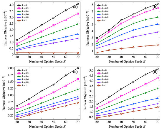
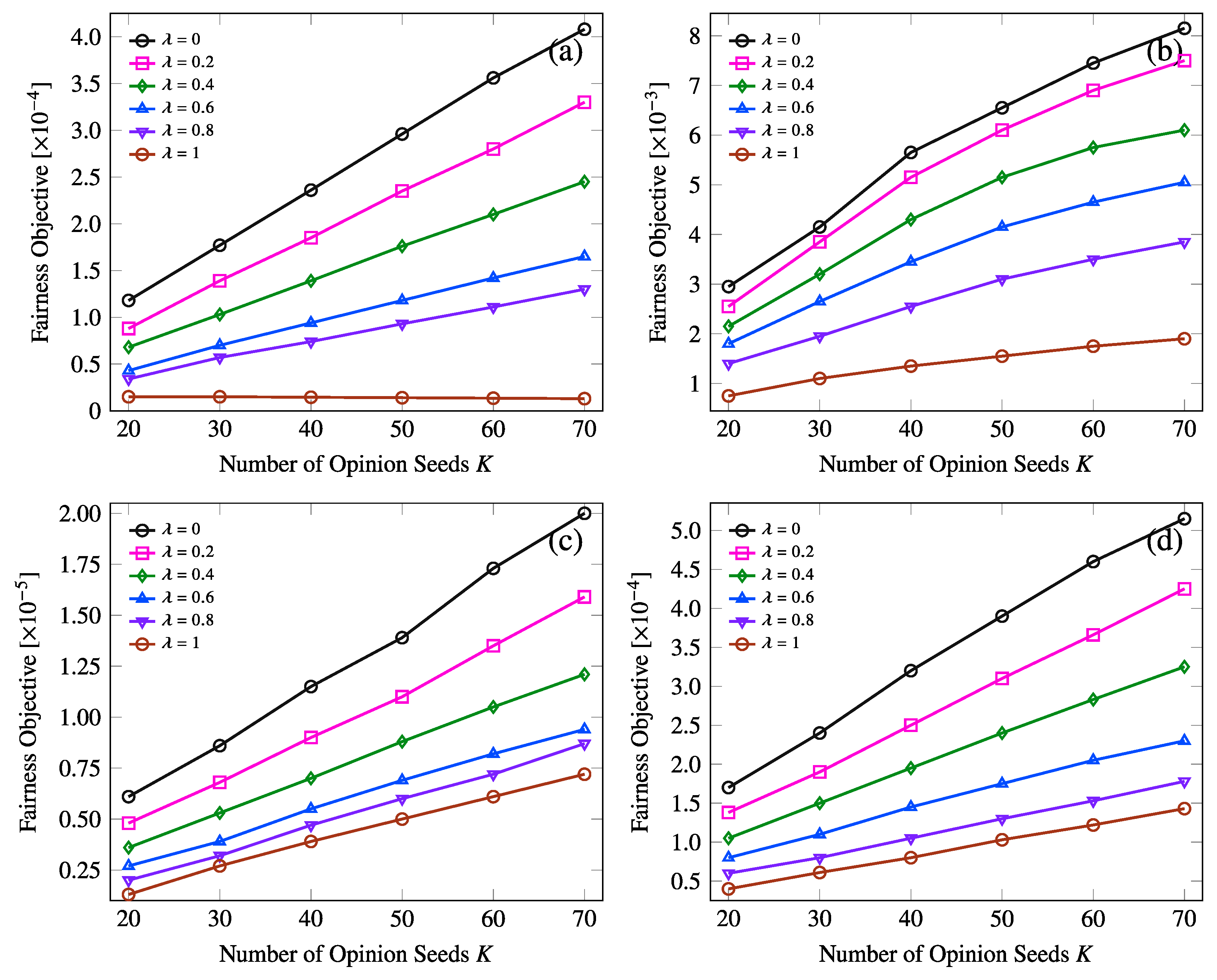
Figure 1 studies the effect of the fairness parameter $\lambda$. For each dataset, the horizontal axis represents the budget K, and the vertical axis represents the optimized fairness-aware objective ${\mathrm{\Phi }}_{\lambda }\left(S\right)$. Each curve corresponds to one value of $\lambda \in \{0,0.2,0.4,0.6,0.8,1\}$.

Figure 1. Effect of the fairness parameter $\lambda$ on the fairness-aware objective. The horizontal axis is the budget K, and the vertical axis is ${\mathrm{\Phi }}_{\lambda }\left(S\right)$. Each curve corresponds to a different value of $\lambda \in \{0,0.2,0.4,0.6,0.8,1\}$. Panels (a–d) show the results on WikiSignedNet, WikiElections, Signed-LiveJournal-2, and WikiSigned, respectively.

For a fixed value of $\lambda$, the objective value generally increases as the budget increases because more seeds provide additional opportunities to improve the equilibrium response. However, objective values corresponding to different $\lambda$ values should not be interpreted as directly comparable, since changing $\lambda$ changes the optimization criterion itself.

The endpoint $\lambda =0$ corresponds to pure global-gain maximization, whereas $\lambda =1$ corresponds to strict worst-group optimization. Therefore, increasing $\lambda$ shifts the optimization toward protecting the least-improved group. Intermediate values provide a continuous trade-off between aggregate improvement and fairness protection.

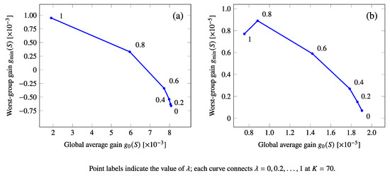
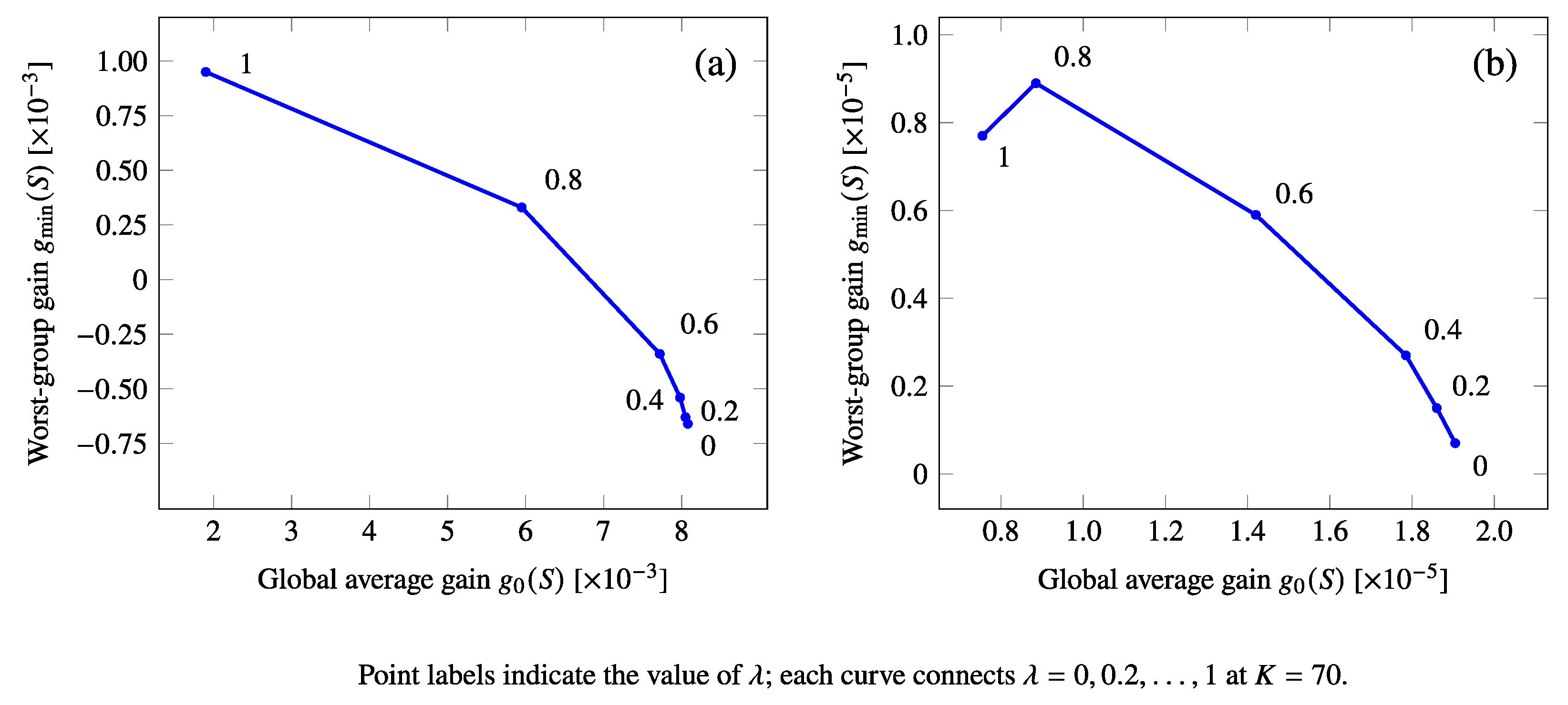
Figure 2 further illustrates this trade-off by plotting the global average gain against the worst-group gain for different values of $\lambda$.

Figure 2. Trade-off between global average gain and worst-group gain under different fairness parameters. (a) WikiElections; (b) Signed-LiveJournal-2.

The results show that fairness-aware opinion seeding does not simply maximize a single influence quantity. Instead, different values of $\lambda$ lead to different operating points between aggregate efficiency and group protection. In particular, when the global-gain solution produces an imbalanced improvement distribution, increasing $\lambda$ can trade part of the global improvement for a higher gain in the least-improved group.

In practice, $\lambda$ can be selected according to application requirements. For example, one can evaluate a prespecified grid of $\lambda$ values and select a value that satisfies an application-dependent lower bound on worst-group improvement while retaining a large global gain.

8.6. Sensitivity to Group Partition Granularity

The fairness-aware objective depends explicitly on the predefined group partition. We therefore examine whether the proposed framework is sensitive to the granularity of the group definition.

As a complementary sensitivity analysis to the default threshold-based grouping strategy described in Section 3, we sort the nodes according to their baseline opinions and partition them into approximately equal-sized groups. Specifically, G2, G3, and G5 correspond to target group proportions of $0.5$, $1/3$, and $0.2$, respectively. These settings represent coarse-, medium-, and fine-grained group partitions. When the number of nodes is not exactly divisible by the number of groups, the resulting group sizes differ by at most one node.

All experiments use AdjointFairGreedy, unit anchoring $\mathsf{\Gamma }=I$, $\lambda =0.5$, and the same candidate sets and budgets as the main experiments.

Table 8 summarizes the results under different levels of group granularity.

Table 8. Sensitivity of fairness-aware opinion seeding to different levels of group granularity. The same candidate sets, budgets, and $\lambda =0.5$ are used in all settings.

Dataset	Groups	Global Gain ${\mathit{g}}_0\left(\mathit{S}\right)$	Worst-Group Gain ${\mathit{g}}_{min}\left(\mathit{S}\right)$	${\mathbf{\Phi }}_{0.5}\left(\mathit{S}\right)$
CongressVotes	G2	0.02301900	−0.00191986	0.01054957
CongressVotes	G3	0.02301900	−0.00159556	0.01071172
CongressVotes	G5	0.02301900	−0.00274177	0.01013862
WikiElections	G2	0.00808138	−0.00048905	0.00379617
WikiElections	G3	0.00806500	−0.00049900	0.00378300
WikiElections	G5	0.00808500	−0.00059700	0.00374400
Signed-LiveJournal-2	G2	0.00001805	0.00000400	0.00001103
Signed-LiveJournal-2	G3	0.00001700	0.00000500	0.00001100
Signed-LiveJournal-2	G5	0.00001900	0.00000200	0.00001000

The results show that the proposed framework remains stable across different levels of group granularity. The global gain remains almost unchanged across these partitions, indicating that the overall improvement is relatively stable.

As the number of groups increases, the worst-group criterion becomes more restrictive, because the minimum is taken over a larger number of groups. Consequently, the worst-group gain may decrease for finer partitions. Nevertheless, the fairness-aware objective remains at a comparable level across all tested granularities, suggesting that the proposed framework is not tied to a specific group resolution.

8.7. Sensitivity to Heterogeneous Anchoring

Table 9 compares unit anchoring, random heterogeneous anchoring, and degree-dependent anchoring. We use $K=6$ for CongressVotes and $K=70$ for WikiElections and Epinions, with $\lambda =0.5$ throughout.

Table 9. Effect of heterogeneous anchoring strengths on AdjointFairGreedy. Random anchoring uses seed 2026; overlap is measured against the unit-anchoring seed set.

Dataset	Anchoring	Global Gain	Worst-Group Gain	${\mathbf{\Phi }}_{0.5}$	Overlap
CongressVotes	Unit	0.02290943	−0.00152682	0.01069131	1.0000
CongressVotes	Random	0.02241599	−0.00125863	0.01057868	1.0000
CongressVotes	Degree-dependent	0.01726472	0.00043987	0.00885229	0.8333
WikiElections	Unit	0.00807213	−0.00048665	0.00379274	1.0000
WikiElections	Random	0.00803926	−0.00049789	0.00377069	0.9429
WikiElections	Degree-dependent	0.00600834	−0.00035516	0.00282659	0.9714
Epinions	Unit	0.00061583	0.00007916	0.00034750	1.0000
Epinions	Random	0.00065279	0.00008063	0.00036671	0.6714
Epinions	Degree-dependent	0.00046836	0.00009038	0.00027937	0.8143

Under unit anchoring, ${\gamma }_i=1$ for every node. For the random heterogeneous setting, the anchoring strengths are sampled independently as

$${\gamma }_i\sim Unif(0.5,1.5),$$

using random seed 2026. For the degree-dependent setting, we define

$${\gamma }_i=0.5+{\displaystyle \frac{\log (1+d_i)}{{max}_j\log (1+d_j)}},d_i=\sum _j\left|A_{ij}\right|.$$

Thus, nodes with larger absolute signed degree are assigned greater anchoring strength. These settings are intended as representative sensitivity scenarios rather than empirically calibrated models of individual resistance.

The overlap between a heterogeneous-anchoring seed set and the corresponding unit-anchoring seed set is defined as

$$Overlap(S_{\mathsf{\Gamma }},S_I)={\displaystyle \frac{|S_{\mathsf{\Gamma }}\cap S_I|}{K}},$$

where $S_I$ is selected under unit anchoring and $S_{\mathsf{\Gamma }}$ is selected under the corresponding heterogeneous setting.

All settings are evaluated using AdjointFairGreedy with identical candidate sets. Changing $\mathsf{\Gamma }$ modifies only the diagonal of the shifted system matrix $M=\mathsf{\Gamma }+\mathcal{L}$; it does not change the sparsity pattern, the number of group-level adjoint solves, or the asymptotic complexity of the algorithm. Nevertheless, different anchoring strengths may affect the conditioning of M and hence the practical cost of the numerical solves. Because separate runtime measurements were not collected for this sensitivity experiment, we restrict the comparison to equilibrium gains, objective values, and selected seeds. We therefore do not claim that heterogeneous anchoring leaves wall-clock time unchanged.

The results show that heterogeneous anchoring can change both the equilibrium response and the selected seeds. Under random anchoring, the CongressVotes seed set remains unchanged, while the overlap is $0.9429$ for WikiElections and $0.6714$ for Epinions. Thus, random anchoring changes four of the 70 selected nodes on WikiElections and retains 47 of the 70 selected nodes on Epinions.

Degree-dependent anchoring changes the fairness–efficiency balance on all three datasets. Compared with unit anchoring, it improves the worst-group gain but reduces the global gain and the resulting value of ${\mathrm{\Phi }}_{0.5}$. This behavior illustrates that stronger anchoring at highly connected nodes can protect the least-improved group while weakening aggregate intervention propagation.

These results show that the framework is not restricted to the unit-anchoring case $\mathsf{\Gamma }=I$. It supports heterogeneous anchoring without changing the gain decomposition or the adjoint algorithm, although the anchoring specification can substantially affect equilibrium gains and the selected seeds.

8.8. Budget Sensitivity and Baseline Comparison

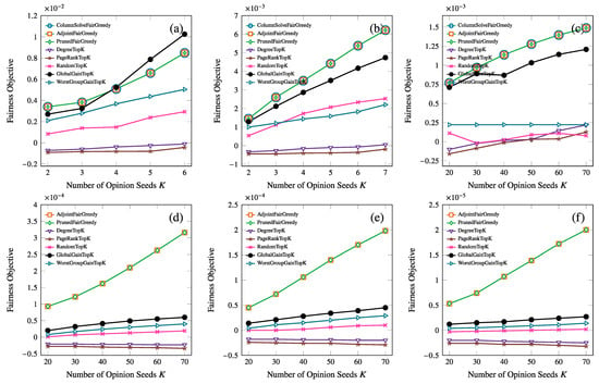
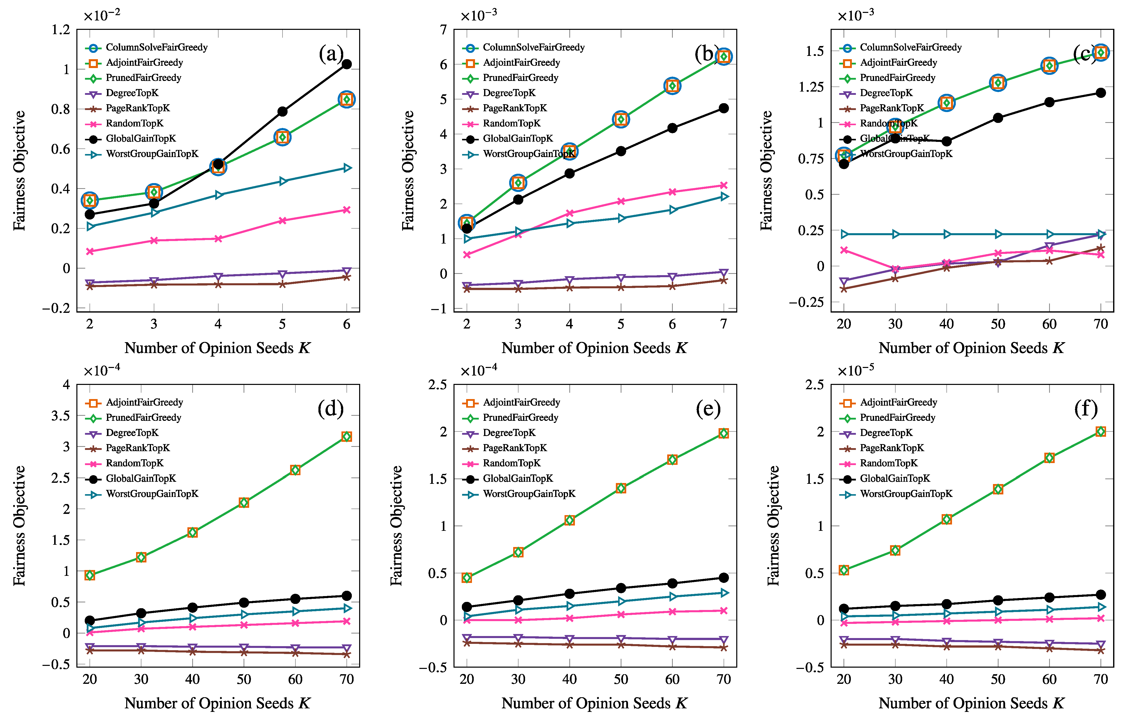
Figure 3 compares the achieved objective values of different selection methods as the exact budget K varies at $\lambda =0.5$. Panels (a)–(f) show CongressVotes, Unicode-Language, Bitcoin-OTC, Epinions, WikiSignedNet, and Signed-LiveJournal-2, respectively, covering networks ranging from hundreds of nodes to more than four million nodes.

Figure 3. Fairness-aware objective as a function of the exact budget K at $\lambda =0.5$. Panels (a–f) show CongressVotes, Unicode-Language, Bitcoin-OTC, Epinions, WikiSignedNet, and Signed-LiveJournal-2, respectively. The six panels compare ColumnSolveFairGreedy, AdjointFairGreedy, and PrunedFairGreedy with degree-, PageRank-, random-, global-gain-, and worst-group-gain-based Top-K baselines. Negative objective values are valid in signed networks because the worst-group gain can be negative; values close to zero may also result from normalization on large networks.

All methods use the same candidate set within each dataset and return exactly K selected seeds. The three fairness-aware implementations are compared with two structural baselines, DegreeTopK and PageRankTopK; one random baseline, RandomTopK; and the stronger target-aware baselines GlobalGainTopK and WorstGroupGainTopK. The exact comparison on small instances is reported separately in Table 10.

Table 10. Certified MILP objective values and relative optimality gaps of the scalable greedy methods on small full-candidate instances.

Dataset	K	MILP Optimum	AFG Gap (%)	PFG Gap (%)
CongressVotes	3	0.005784470769	7.4343	7.4343
CongressVotes	5	0.009458083724	0.0000	0.0000
CongressVotes	7	0.011921524158	0.0000	0.0000
Unicode-Language	3	0.002651013139	0.0000	0.0000
Unicode-Language	5	0.004223336387	0.0000	0.0000
Unicode-Language	7	0.005726979687	0.0000	0.0000

The three fairness-aware implementations produce identical or visually indistinguishable objective curves across all tested datasets. This agreement, together with the residual validation in Table 6, shows that the adjoint formulation reproduces the reference objective values to numerical precision. The numerical validation also yields identical selected sets for all tested small-instance budgets; the only observed ordering difference is a swap between two nearly tied candidates on CongressVotes. Thus, the scalable implementations do not obtain their computational advantages by changing the underlying fairness-aware objective.

The target-aware baselines provide a stronger comparison than purely structural rankings because they use the same signed Friedkin–Johnsen response information as the proposed method. GlobalGainTopK selects nodes with large singleton global gains, whereas WorstGroupGainTopK focuses on singleton worst-group improvement. However, both methods optimize only one component of the fairness-aware objective and ignore the interaction among multiple selected seeds.

The proposed greedy rule directly optimizes

$${\mathrm{\Phi }}_{\lambda }\left(S\right)=(1-\lambda )g_0\left(S\right)+\lambda g_{min}\left(S\right),$$

and therefore balances aggregate improvement with worst-group protection. The comparison should be interpreted as a trade-off analysis rather than a claim of universal dominance, since the fairness-aware objective is not submodular in general.

The structural baselines behave differently. DegreeTopK and PageRankTopK rank nodes according to connectivity information from the unsigned magnitude graph and do not consider edge signs, baseline opinions, or group-level gains. Consequently, a highly central node is not necessarily an effective fairness-aware opinion seed. Its intervention may propagate through positive and negative signed paths differently and may improve one group while harming another.

The small numerical magnitudes observed on WikiSignedNet and Signed-LiveJournal-2 should be interpreted according to the normalized objective. The global gain and group gains are averages, whereas the number of selected seeds is small compared with the network size. Therefore, localized equilibrium changes can lead to average gains of order ${10}^{-5}$ or smaller. Such values represent valid but small effects rather than failed computations.

RandomTopK generally remains below the optimization-based methods as the budget increases. Although random selection may occasionally avoid unfavorable structural biases, it does not exploit signed propagation or fairness information. This behavior reflects the fact that random selection does not use signed propagation or group-level gain information.

8.9. MILP Optimality Gap on Small Instances

To evaluate the solution quality of the scalable greedy methods, we compare their solutions with the exact mixed-integer linear formulation introduced in Section 5. The experiments are conducted on CongressVotes and Unicode-Language, for which the complete candidate sets are used, i.e., $C=V$. We set $\mathsf{\Gamma }=I$ and $\lambda =0.5$, and evaluate $K\in \{3,5,7\}$.

To match the fixed-budget setting used throughout the experiments, the MILP uses the exact-cardinality constraint

$$\sum _{u\in C}{x}_u=K.$$

The relative optimality gap is defined as

$$Gap\left(S\right)=100{\displaystyle \frac{{\mathrm{\Phi }}^{★}-\mathrm{\Phi }\left(S\right)}{|{\mathrm{\Phi }}^{★}|}}\%,$$

where ${\mathrm{\Phi }}^{★}$ denotes the certified MILP optimum.

The results show that both scalable greedy implementations achieve the certified MILP optimum in five of the six tested settings. The only nonzero gap occurs on CongressVotes with $K=3$, where the relative gap is $7.4343\%$. This gap disappears when the budget increases to $K=5$ and $K=7$.

These results do not establish a worst-case approximation guarantee, since the fairness-aware objective is generally non-submodular. Instead, they provide empirical evidence that the proposed greedy strategies are close to the global optimum on instances where exact verification is possible.

The identical gaps of AdjointFairGreedy and PrunedFairGreedy are consistent with the sequence-preservation property of Pareto dominance pruning under the stated dominance and tie rules.

8.10. Summary of Findings

The experiments support eight main conclusions.

First, the running-time comparison demonstrates that AdjointFairGreedy scales most robustly among the tested implementations. The column-solve method serves as a reference implementation but becomes expensive because it requires candidate-wise response computations.

Second, the numerical validation shows that the column-solve and adjoint implementations have small residuals and agree to approximately ${10}^{-13}$ in candidate gains and ${10}^{-14}$ in achieved objective values. The observed discrepancies are substantially below the residual-based theoretical bounds, providing empirical support for the numerical error analysis.

Third, the Pareto pruning analysis explains the instance-dependent behavior of PrunedFairGreedy. Compact nondominated frontiers allow large candidate reductions, whereas large frontiers may introduce additional dominance-checking and maintenance overhead.

Fourth, the fairness-parameter experiments show that $\lambda$ provides an interpretable mechanism for balancing global average improvement and worst-group protection. The corresponding trade-off curves reveal the practical meaning of fairness-aware optimization.

Fifth, the group-partition sensitivity experiment shows that the framework remains effective across different levels of group granularity. Although finer partitions make the worst-group criterion more restrictive, the overall fairness-aware objective remains stable.

Sixth, the heterogeneous-anchoring experiment shows that the proposed framework naturally supports node-dependent anchoring strengths. Different anchoring structures can affect both selected seeds and the fairness–efficiency balance.

Seventh, the baseline comparison shows that the performance of the proposed method is not solely due to weak structural baselines. Target-aware baselines use signed Friedkin–Johnsen information but optimize only individual components, whereas the proposed method directly optimizes their combination.

Finally, the MILP comparison on small full-candidate instances shows that the scalable greedy methods achieve solutions close to certified global optima while remaining applicable to large signed networks. Overall, the experiments show that the proposed framework provides a scalable and flexible approach for fairness-aware opinion seeding in signed Friedkin–Johnsen networks.

9. Extensions and Discussion

9.1. Weighted Group Welfare

The framework also permits application-dependent node weights. For nonnegative weights ${\omega }_i$, assume

$${\mathrm{\Omega }}_a=\sum _{j\in V_a}{\omega }_j>0,\mathrm{\Omega }=\sum _{j\in V}{\omega }_j,$$

and define

$$h_a^{\omega }\left(i\right)=\left\{\begin{array}{cc}{\displaystyle \frac{{\omega }_i}{{\mathrm{\Omega }}_a},}\hfill & i\in V_a,\hfill \\ 0,\hfill & i\notin V_a.\hfill \end{array}\right.$$

If global welfare is weighted consistently, set $h_0^{\omega }\left(i\right)={\omega }_i/\mathrm{\Omega }$ and $p_a^{\omega }={\mathrm{\Omega }}_a/\mathrm{\Omega }$. Then

$$h_0^{\omega }={\displaystyle \sum _{a=1}^r}{p}_a^{\omega }{h}_a^{\omega },$$

so the global adjoint remains redundant and only the right-hand sides and group proportions change. Degree, inverse degree, PageRank, betweenness, forest centrality, or resistance-based weights can therefore be incorporated without changing the optimization framework. If the global average is intentionally kept unweighted while the group averages are weighted, this identity generally fails and one additional global adjoint solve is required.

9.2. Interpretation and Limitations

The model separates three layers that should not be conflated. The signed Friedkin–Johnsen system specifies how interventions propagate. The group partition specifies whose average outcomes are compared. The candidate set specifies who is eligible for intervention. Stratified candidate construction may improve group representation, but it also restricts the feasible set and can exclude a globally optimal seed set.

The fairness objective is neither monotone nor submodular in general. Consequently, greedy selection is a computational heuristic, and its quality should be evaluated against the mixed-integer optimum whenever possible. Dynamic dominance pruning is exact relative to the stated greedy and tie rules, but its speedup is data-dependent and may disappear when most gain vectors are mutually nondominated.

The primary analysis assumes an undirected signed graph. Directed signed networks lead to nonsymmetric systems and require separate conditions for invertibility, stability, and numerical solution. Extending the residual analysis and the intervention model to that setting is an important direction for future work.

Finally, opinion-based groups are useful when only a signed network is available, but they measure balance across opinion strata rather than fairness with respect to protected attributes. Applications involving demographic fairness require externally justified group labels and an appropriate ethical interpretation of the intervention. Setting an individual’s internal opinion to $+1$ represents a strong and potentially manipulative intervention; the target stance is not intrinsically beneficial. Real deployments would additionally require a legitimate purpose, consent or other appropriate authorization, safeguards against coercion, and sensitivity analysis for misspecified edge signs, anchoring strengths, and group labels.

10. Conclusions

We formulated fairness-aware internal-opinion seeding in undirected signed Friedkin–Johnsen networks with heterogeneous anchoring strengths. The objective balances the global average equilibrium gain with the minimum group-average gain. By exploiting the linearity of the equilibrium response, we showed that each candidate can be represented by an r-dimensional group-gain vector and that the global gain is a size-weighted combination of the group gains. This representation leads to an exact mixed-integer linear program for tractable instances and an adjoint formulation requiring only one shifted signed-Laplacian solve per group. We also introduced a dynamically maintained Pareto frontier based on componentwise dominance, which can preserve the underlying greedy sequence under the stated dominance and tie conditions.

The theoretical analysis establishes the well-posedness and stability of the signed Friedkin–Johnsen equilibrium, correctness of the candidate-gain and adjoint formulations, sufficient conditions for monotonicity, non-submodularity of the fairness-aware objective in general, residual-based numerical error bounds, and computational complexity. These results clarify both the strengths and the limitations of the proposed framework: group-aware interventions in signed networks can be evaluated efficiently, but the max–min coupling introduces candidate complementarity and prevents direct application of classical monotone-submodular approximation guarantees. The best-prefix rule also allows the at-most-k greedy heuristic to continue through nonimproving intermediate prefixes without implying global optimality.

Empirically, the adjoint implementation scales most robustly among the tested methods on 14 signed networks ranging from hundreds to more than four million nodes. The experiments also show that the fairness parameter and heterogeneous anchoring strengths can substantially affect both the selected seed sets and the balance between global average gain and worst-group gain. Compared with structural, random, and target-aware Top-K baselines, the proposed greedy method remains broadly competitive. On the two small full-candidate networks used for exact verification, the scalable greedy methods match the solver-certified MILP optimum in five of the six tested configurations, with the only nonzero relative gap equal to 7.4343% on CongressVotes at $K=3$. These results provide empirical support for the practical scalability and solution quality of the framework, without implying a general worst-case approximation guarantee.

Future work includes directed and time-varying signed systems, multilayer networks, continuous or partial interventions, fairness criteria beyond weighted max–min welfare, and algorithms with stronger instance-dependent or problem-specific approximation guarantees.

References

- Leskovec, J.; Huttenlocher, D.; Kleinberg, J. Signed Networks in Social Media. In Proceedings of the SIGCHI Conference on Human Factors in Computing Systems; ACM: New York, NY, USA, 2010; pp. 1361–1370. [Google Scholar] [CrossRef] [Scilit]
- Kunegis, J.; Lommatzsch, A.; Bauckhage, C. The Slashdot Zoo: Mining a Social Network with Negative Edges. In Proceedings of the 18th International Conference on World Wide Web; ACM: New York, NY, USA, 2009; pp. 741–750. [Google Scholar] [CrossRef] [Scilit]
- Altafini, C. Consensus Problems on Networks with Antagonistic Interactions. IEEE Trans. Autom. Control 2013, 58, 935–946. [Google Scholar] [CrossRef] [Scilit]
- Zhou, X.; Sun, H.; Xu, W.; Li, W.; Zhang, Z. Friedkin–Johnsen Model for Opinion Dynamics on Signed Graphs. IEEE Trans. Knowl. Data Eng. 2024, 36, 8313–8327. [Google Scholar] [CrossRef] [Scilit]
- DeGroot, M.H. Reaching a Consensus. J. Am. Stat. Assoc. 1974, 69, 118–121. [Google Scholar] [CrossRef]
- Friedkin, N.E.; Johnsen, E.C. Social Influence and Opinions. J. Math. Sociol. 1990, 15, 193–206. [Google Scholar] [CrossRef] [Scilit]
- Friedkin, N.E.; Johnsen, E.C. Social Influence Network Theory: A Sociological Examination of Small Group Dynamics; Cambridge University Press: Cambridge, UK, 2011. [Google Scholar]
- Gionis, A.; Terzi, E.; Tsaparas, P. Opinion Maximization in Social Networks. In Proceedings of the 2013 SIAM International Conference on Data Mining; SIAM: Philadelphia, PA, USA, 2013; pp. 387–395. [Google Scholar] [CrossRef] [Scilit]
- Musco, C.; Musco, C.; Tsourakakis, C.E. Minimizing Polarization and Disagreement in Social Networks. In Proceedings of the 2018 World Wide Web Conference; ACM: New York, NY, USA, 2018; pp. 369–378. [Google Scholar] [CrossRef] [Scilit]
- Xu, P.; Hu, W.; Wu, J.; Liu, W. Opinion Maximization in Social Trust Networks. In Proceedings of the Twenty-Ninth International Joint Conference on Artificial Intelligence; International Joint Conferences on Artificial Intelligence Organization: California City, CA, USA, 2020; pp. 1251–1257. [Google Scholar] [CrossRef] [Scilit]
- Out, C.; Tu, S.; Neumann, S.; Zehmakan, A.N. The Impact of External Sources on the Friedkin–Johnsen Model. In Proceedings of the 33rd ACM International Conference on Information and Knowledge Management; ACM: New York, NY, USA, 2024; pp. 1815–1824. [Google Scholar] [CrossRef] [Scilit]
- Zhu, L.; Zhang, Z. Opinion Maximization in Social Networks via Link Recommendation. Theor. Comput. Sci. 2025, 1033, 115090. [Google Scholar] [CrossRef] [Scilit]
- Sun, H.; Zhang, Z. Opinion Optimization in Directed Social Networks. Proc. AAAI Conf. Artif. Intell. 2023, 37, 4623–4632. [Google Scholar] [CrossRef] [Scilit]
- Sun, H.; Zhang, Z. Leader Selection for Opinion Optimization in Social Networks. Theor. Comput. Sci. 2026, 1073, 115894. [Google Scholar] [CrossRef] [Scilit]
- Kempe, D.; Kleinberg, J.; Tardos, É. Maximizing the Spread of Influence through a Social Network. In Proceedings of the Ninth ACM SIGKDD International Conference on Knowledge Discovery and Data Mining; ACM: New York, NY, USA, 2003; pp. 137–146. [Google Scholar] [CrossRef] [Scilit]
- Tsang, A.; Wilder, B.; Rice, E.; Tambe, M.; Zick, Y. Group-Fairness in Influence Maximization. In Proceedings of the Twenty-Eighth International Joint Conference on Artificial Intelligence; International Joint Conferences on Artificial Intelligence Organization: California City, CA, USA, 2019; pp. 5997–6005. [Google Scholar] [CrossRef] [Scilit]
- Farnad, G.; Babaki, B.; Gendreau, M. A Unifying Framework for Fairness-Aware Influence Maximization. In Proceedings of the Web Conference 2020 Companion; ACM: New York, NY, USA, 2020; pp. 714–722. [Google Scholar] [CrossRef] [Scilit]
- Rahmattalabi, A.; Jabbari, S.; Lakkaraju, H.; Vayanos, P.; Izenberg, M.; Brown, R.; Rice, E.; Tambe, M. Fair Influence Maximization: A Welfare Optimization Approach. Proc. AAAI Conf. Artif. Intell. 2021, 35, 11630–11638. [Google Scholar] [CrossRef] [Scilit]
- Becker, R.; D’Angelo, G.; Ghobadi, S. On the Cost of Demographic Parity in Influence Maximization. Proc. AAAI Conf. Artif. Intell. 2023, 37, 14110–14118. [Google Scholar] [CrossRef] [Scilit]
- Chowdhary, S.; De Pasquale, G.; Lanzetti, N.; Stoica, A.A.; Dörfler, F. Fairness in Social Influence Maximization via Optimal Transport. In Proceedings of the 38th Conference on Neural Information Processing Systems (NeurIPS 2024); Curran Associates, Inc.: Red Hook, NY, USA, 2024; Volume 37. [Google Scholar] [CrossRef] [Scilit]
- Zhai, Y.; Han, Z.; Dong, Z.; Yang, X.; Wang, B. Opinion Maximization Based on Fairness in Social Networks. Data Sci. Eng. 2026, 11, 84–99. [Google Scholar] [CrossRef] [Scilit]
- Papachristou, M.; Kleinberg, J. Quantifying and Mitigating Consensus Disparity in Social and Information Networks. SSRN Electron. J. 2026. [Google Scholar] [CrossRef] [Scilit]
- Theologis, N.; Pitoura, E.; Terzi, E.; Tsaparas, P. Fairness in Opinion-Formation Dynamics. In Proceedings of the ACM Web Conference 2026; ACM: New York, NY, USA, 2026; pp. 4841–4852. [Google Scholar] [CrossRef] [Scilit]
- Miyauchi, A.; Kuroki, Y.; Cinus, F.; Neumann, S.; Bonchi, F. A Survey on Algorithmic Interventions in Opinion Dynamics. arXiv 2026, arXiv:2603.10756. [Google Scholar] [CrossRef] [Scilit]
- Razaq, M.A.; Altafini, C. Signed Friedkin–Johnsen Models: Opinion Dynamics with Stubbornness and Antagonism. IEEE Trans. Autom. Control 2025, 70, 5037–5051. [Google Scholar] [CrossRef] [Scilit]
- Zhou, X.; Zhou, X.; Li, Y.; Zhang, Z. Fast Leader Selection for Opinion Maximization in Signed Graphs. Theor. Comput. Sci. 2026, 1069, 115817. [Google Scholar] [CrossRef] [Scilit]
- Spielman, D.A.; Teng, S.H. Nearly Linear Time Algorithms for Preconditioning and Solving Symmetric, Diagonally Dominant Linear Systems. SIAM J. Matrix Anal. Appl. 2014, 35, 835–885. [Google Scholar] [CrossRef] [Scilit]
- Li, W.; Bai, W.; Cao, J. Turing instability and pattern formation in a diffusive predator-prey system with opportunistic predators and weak Allee effect. Phys. Rev. E 2026, 113, 044219. [Google Scholar] [CrossRef] [Scilit]
- Li, W.; Zhang, Y.; Ding, Q.; Yu, J. Exponential convergence of a diffusive SIRS epidemic model with standard incidence. J. Geom. Anal. 2026, 36, 13. [Google Scholar] [CrossRef] [Scilit]
- Hou, Y.P. Bounds for the Least Laplacian Eigenvalue of a Signed Graph. Acta Math. Sin. Engl. Ser. 2005, 21, 955–960. [Google Scholar] [CrossRef] [Scilit]
- Merris, R. Laplacian Matrices of Graphs: A Survey. Linear Algebra Its Appl. 1994, 197–198, 143–176. [Google Scholar] [CrossRef] [Scilit]
- Spielman, D.A.; Teng, S.H. Nearly-Linear Time Algorithms for Graph Partitioning, Graph Sparsification, and Solving Linear Systems. In Proceedings of the Thirty-Sixth Annual ACM Symposium on Theory of Computing; ACM: New York, NY, USA, 2004; pp. 81–90. [Google Scholar] [CrossRef] [Scilit]
- Kyng, R.; Sachdeva, S. Approximate Gaussian Elimination for Laplacians: Fast, Sparse, and Simple. In Proceedings of the 57th Annual IEEE Symposium on Foundations of Computer Science; IEEE: New York, NY, USA, 2016; pp. 573–582. [Google Scholar] [CrossRef] [Scilit]
- Lu, Z.; Xu, W.; Zhang, Z. Diagonal of Pseudoinverse of Graph Laplacian: Fast Estimation and Exact Results. Theor. Comput. Sci. 2025, 1032, 115102. [Google Scholar] [CrossRef] [Scilit]
- Nemhauser, G.L.; Wolsey, L.A.; Fisher, M.L. An Analysis of Approximations for Maximizing Submodular Set Functions—I. Math. Program. 1978, 14, 265–294. [Google Scholar] [CrossRef] [Scilit]
Disclaimer/Publisher’s Note: The statements, opinions and data contained in all publications are solely those of the individual author(s) and contributor(s) and not of MDPI and/or the editor(s). MDPI and/or the editor(s) disclaim responsibility for any injury to people or property resulting from any ideas, methods, instructions or products referred to in the content. |
© 2026 by the authors. Licensee MDPI, Basel, Switzerland. This article is an open access article distributed under the terms and conditions of the Creative Commons Attribution (CC BY) license.