


Abstract
Brushless DC (BLDC) motors are the preferred traction drive for electric vehicles (EVs), yet achieving precise speed regulation and low torque ripple under varying loads and nonlinear dynamics remains challenging. This paper proposes a cascaded control architecture for BLDC drives under Field-Oriented Control (FOC) in which a Self-Tuning Fuzzy Logic Controller (ST-FLC) continuously adapts the gains of Two-Degree-of-Freedom Proportional-Integral (2DOF-PI) controllers governing both the outer speed loop and the inner d-q current loops. The FLC membership functions and scaling factors are optimized offline by four metaheuristics, namely the Basketball Team Optimization Algorithm (BTOA), Piranha Foraging Optimization Algorithm (PFOA), Pufferfish Optimization Algorithm (POA), and Firefighter Optimization Algorithm (FFO), to minimize an Integral Squared Error (ISE) criterion. MATLAB/Simulink(R2025b) results show that the BTOA-tuned ST-FLC–2DOF-PI controller attains the lowest ISE (2776) and outperforms BTOA-tuned PI, 2DOF-PI, and FLC benchmarks, achieving a 3.5 ms settling time (65% faster than PI), 0.5% overshoot, zero steady-state speed error, the lowest steady-state torque ripple of 15%, and the lowest phase-current THD of 6.28%. Performance is maintained under ±50% parameter variations, and Bode analysis confirms phase margins of 63.4° and 101° for the speed and current loops. Hardware-in-the-Loop validation on an OPAL-RT real-time simulator closely matches the offline simulations, confirming real-time implementability.
Keywords:
self-tuning fuzzy logic controller; 2DOF-PI; torque ripple reduction; BLDC motor; field-oriented control; THD; electric vehicles; metaheuristic optimizations; speed control MSC:
35B38; 74G65; 74H80
1. Introduction
Transportation is moving away from fossil fuels, and electric vehicles (EVs) have become the leading alternative for cutting greenhouse gas emissions. The International Energy Agency counted more than 40 million EVs on the road in 2023 and expects that number to climb sharply over the coming decade, helped along by better motors, batteries, charging infrastructure, and control systems [1]. The core of any electric vehicle lies in its electric propulsion system, which relies on a brushless DC (BLDC) motor to convert electrical energy into the mechanical energy that drives the vehicle. Since the motor must deliver high performance under diverse driving conditions—including startup, acceleration, constant and variable speed cruising, hill climbing and descending, and frequent braking—energy efficiency, precise speed control, and smooth torque generation are fundamental pillars of vehicle performance [2]. These three elements form the basis for developing BLDC motor control systems; consequently, designing an appropriate control strategy and selecting the right motor are critical decisions in the electric vehicle development process.
Brushless DC (BLDC) motors have outperformed other types of motors in electric vehicle traction applications, including induction motors, wound-field synchronous motors, permanent magnet synchronous motors, and variable frequency drives. This is due to their high efficiency, energy density, small size, and low maintenance requirements. The absence of brushes or mechanical commutators means less friction and wear, and a longer service life. Therefore, BLDC motors have become widely used not only in traction systems but also in electric vehicle subsystems such as electric power steering and air conditioning [2,3,4]. Continued advances in power electronics and permanent magnet materials have also directly contributed to improving the performance of BLDC motors [5,6].
However, optimal control of a brushless DC motor is not easy. Moreover, because a BLDC motor is non-linear and operates under varying loads, temperatures, and parameters, maintaining a constant speed under rapidly changing conditions is a significant challenge [7,8]. Not only is torque ripple caused by switching effects and the interaction between the rotor and stator magnets a persistent problem that results in harmonics [7,8], but excessive ripple also leads to vibrations, mechanical stress, and noise, negatively impacting both driving and ride comfort [9,10]. Any practical control strategy must deliver strong dynamic performance despite all of this.
Field-Oriented Control (FOC), or vector control, is the standard route to high-performance BLDC and PMSM drives. Using the Clarke and Park transforms, it maps the three-phase currents onto a rotating frame aligned with the rotor flux, splitting them into a flux-generating (id) and a torque-generating (iq) component that can be regulated quickly and independently, much like a separately excited DC motor. Paired with space-vector pulse-width modulation (SVPWM), FOC produces near-sinusoidal currents with less torque ripple and harmonic distortion than conventional six-step switching [11,12], and it runs comfortably on low-cost microcontrollers and FPGAs, scaling to other machine types such as multi-stage motors (MSMs) and double-stator motors (DSMs) [13,14]. Inside the FOC loops, Proportional Integral (PI) controllers still dominate industry practice because they are simple and cheap to tune [15]. The catch is that a fixed PI is only appropriate at the operating point it was tuned for, and an EV motor rarely stays there. Not only does speed control become more difficult but also controlling the moment of inertia and load torque during hill climbing, braking, and off-road driving. Controlling current during braking and at low speeds is particularly challenging as the reverse electromotive force approaches the resistive voltage drop. Gain values high enough to reject load disturbances lead to overshoots during speed changes, while low gain values smooth the response but react slowly to load changes—a classic trade-off between tracking and rejection [16,17]. Parameter deviations across the operating range further exacerbate this imbalance [18]. For these reasons, adaptive control strategies have become necessary to bridge the gap between a single set point and the actual driving dynamics of an electric vehicle [19].
The PI two-degrees of freedom (2DOF) structure solves half of this problem by separating the reference path from the feedback path, i.e., separating command tracking from disturbance rejection so that each can be set separately [20]. The idea has a solid track record in motor drives: global exponential stability and stronger disturbance rejection in PMSM drives [21], improved dynamics with a PSO-tuned 2DOF-PI inside the FOC loop [22], and faster, better-damped transients in both PMSM and BLDC drives [23,24]. What it does not fix is adaptability. Its gains stay constant and its action is linear, so the decoupling only holds near the point it was tuned for; once speed, load, or inertia moves, a fixed 2DOF-PI drifts off just like an ordinary PI.
Fuzzy logic controllers (FLCs) bring the missing adaptability. Because they encode control action as “if-then” rules instead of a fixed transfer function, they cope with the nonlinearity and uncertainty that defeat linear controllers [25], and fuzzy-based drives have shown measurable gains in torque-ripple reduction and transient response [26,27,28,29,30]. However, traditional fuzzy logic control (FLC) systems are not self-tuning: their measurement parameters and belonging functions are fixed at the design stage, resulting in decreased performance as the operating point changes. Self-tuning FLCs (ST-FLCs), on the other hand, adjust these parameters in real time [31] and consistently outperform their fixed counterparts [32,33,34]. However, the structural safeguards offered by linear design are lost, as the FLC itself does not provide a direct path to stability margins or a separate track from rejection. Furthermore, published studies on self-tuning FLCs typically pair the fuzzy phase with a simple PI loop; its integration with a structural controller, such as the proposed 2DOF-PI, has rarely been tested.
Setting up such a microcontroller is a complex optimization issue because the input/output scaling factors and ST-FLC membership functions form a high-dimensional, non-convex search space filled with local minimums. There is no gradient information to guide the search, which is typical of population-based meta-algorithms [35]. Experiments with algorithms such as PSO, GA, and GWO show that the results depend heavily on how each algorithm balances local exploitation and global exploration, and on how the cost function is formulated [36]. Although they still outperform manual and traditional tuning [37], similar observations have been reported for hybrid meta-controller designs, including fractional-order PID microcontrollers [38,39,40]. Optimizer choice matters, in other words, and that motivates trying newer algorithms whose search behaviour may suit the FLC tuning landscape better.
Here, for the first time, four modern algorithms for selecting the best-performing brushless DC motor controller are compared, each offering a different search mechanism. The basketball team optimization algorithm (BTOA) switches player roles between offensive and defensive strategies, moving from omnidirectional exploration to local optimization while continuing to search [41]. The piranha foraging optimization algorithm (PFOA) uses cooperative offensive strategies and an adaptive population structure to continue exploring while converging [42]. The Puffer-fish Optimization Algorithm (POA) divides the search process into two explicit phases: exploration and exploitation, inspired by the natural defensive behaviour of the pufferfish [43]. The Firefighter Optimization Algorithm (FFO), on the other hand, is inspired by emergency responses and has performed competitively on standard benchmark problems [44]. Not only have neither of these algorithms been previously applied to the design of drive motor control units but determining the most suitable search behaviour for tuning an FLC system is an open question that this study addresses empirically. The choice of these four algorithms is methodological rather than designed to search for the algorithm with the highest score. Classical optimizers such as PSO, GA and DE are already well characterized on this class of problem and appear in the studies cited above; they form the reference against which newer search behaviour is judged, and their documented tendency to lose population diversity on high-dimensional multimodal landscapes is precisely the failure mode of interest here. Bayesian optimization was not adopted because it is designed for expensive low-dimensional black-box functions, whereas the present decision vector is high-dimensional and each evaluation is an inexpensive simulation, so the surrogate-model overhead outweighs its benefit. The four algorithms selected instead span four distinct exploration-exploitation mechanisms, so that comparing them isolates which search behaviour suits the FLC tuning landscape rather than merely ranking optimizers.
Hybrid systems combining fuzzy logic and PI-based control offer smoother operation for traction applications compared to traditional methods alone [45,46]. However, the integration of a self-tuning fuzzy logic controller (ST-FLC) with a two-degrees-of-freedom PI-based controller (2DOF-PI) has not been fully implemented within the FOC framework for BLDC motors. Furthermore, none of the four algorithms to be studied have been evaluated for traction tasks using BLDC motors. Current harmonics introduce losses, torque ripple, and electromagnetic interference; therefore, phase current quality is critical [47], and advanced control can significantly improve waveform quality [48,49,50].
Relative to the three families of work closest to this study, the contribution is specific rather than incremental. Compared with adaptive fuzzy controllers, which adjust gains online but are normally built on a single-degree-of-freedom loop with hand-tuned membership functions, the fuzzy adaptation here sits inside a two-degrees-of-freedom cascade and the membership-function shapes are obtained by optimization rather than by expert choice. Compared with 2DOF-PI controllers, which decouple setpoint tracking from disturbance rejection but with gains that are fixed once designed, the proposed scheme retains that decoupling while making the proportional and integral gains, and the setpoint weight functions of the instantaneous error and its rate, so both degrees of freedom remain effective across the operating range rather than only at the design point. Compared with metaheuristic-optimized BLDC controllers, which typically tune a handful of PI gains against a speed-error criterion, the optimization here spans multiple parameters covering the membership-function shapes and the separate speed-loop and current-loop scaling factors, and is driven by a multi-component objective that includes the d- and q-axis current errors alongside the speed error. The novelty is therefore the combination itself: an online-adaptive fuzzy layer and a structurally decoupled 2DOF cascade whose entire parameter set is optimized as a single vector. To our knowledge, this ST-FLC–2DOF-PI combination, together with the first application of the four studied optimizers to BLDC-drive tuning, has not previously been reported for BLDC traction drives. Accordingly, the main contributions of this study are as follows:
- (1)
- The design of a new BTOA-optimized ST-FLC–2DOF-PI controller within the FOC framework for BLDC motor drives in EVs.
- (2)
- The application and comparison of four modern exploratory methods (BTOA, PFOA, POA, and FFO) for selecting the optimal controller for a BLDC, where BTOA proved to be the most effective.
- (3)
- Benchmarking of the proposed controller against BTOA-tuned PI, 2DOF-PI, and FLCs on speed response, torque ripple, and THD of the phase current.
- (4)
- A Bode analysis to check the stability of the system and ensure there is sufficient gain and phase margins.
- (5)
- Validation of the drive system in MATLAB/Simulink and in real time via hardware-in-the-loop (HIL) testing on an OPAL-RT simulator, demonstrating the controller’s effectiveness and its implementability under real-time execution constraints.
The remainder of this paper is structured as follows. Section 2 presents the mathematical formulation of the BLDC motor. Section 3 introduces the proposed ST-FLC–2DOF-PI control architecture and formulates the associated optimization problem, including the BTOA-based tuning procedure. Section 4 details the evaluation of the proposed approach through simulation studies and compares the performance of four optimization algorithms and three reference controllers. Section 5 details the analysis of stability; Section 6 covers the HIL validation on the OPAL-RT platform. Finally, Section 7 summarizes the main findings and outlines potential directions for future research.
2. Mathematical Modeling of the Brushless DC Motor
The BLDC motor may be described as a permanent-magnet synchronous drive in which electronic commutation replaces mechanical commutation, while the stator employs a balanced three-phase winding and the rotor incorporates surface-mounted permanent magnets. Because the rotor is constructed from high-resistance materials, rotor currents are negligible [2]. Figure 1 depicts the equivalent circuit of the three-phase Y-connected BLDC motor. Each phase consists of a phase resistance , self-inductance , mutual inductance , and an induced back-EMF source represented by , , and .
Figure 1.
Equivalent circuit of the three-phase, Y-connected BLDC motor.
2.1. Three-Phase Electrical Model
In fact, the structural similarity between a three-phase synchronous motor and a BLDC motor led to the adoption of a similar modelling approach [51]. By writing Kirchhoff’s voltage law (KVL) for each phase of the circuit in Figure 1, we obtain the motor voltage equations as follows:
Equations (1)–(3) can be written in matrix form as follows:
The differential operator is represented by . To simplify handling the dynamic model, the analysis is based on the following assumptions: equal resistance across phases, minimal loss in the iron core, zero interfacial inductance, and constant self-inductance for each coil:
The potential equations can be simplified by applying these conditions and including the neutral point potential and represented as a matrix:
2.2. Back-Electromotive Force Model
The machine is a three-phase sinusoidal-back-EMF permanent-magnet synchronous machine (PMSM); it therefore generates sinusoidal back-EMF waveforms. The three-phase back-EMFs are functions of the electrical rotor angle and mechanical angular velocity :
where denotes the back-EMF constant [V·rad−1·s−1]; is the normalized sinusoidal back-EMF waveform function , periodic with period and symmetrically phase-shifted by between phases; and is the angle of the electric rotor, where is the number of poles and is the angle of the mechanical rotor.
2.3. Electromagnetic Torque and Mechanical Equations
By dividing the total air-gap power (calculated as the sum of the product of the back-EMF–current products across the three phases) by the mechanical angular velocity, the instantaneous electromagnetic torque is obtained:
Under field-oriented control in the rotor d–q reference frame with , Equation (11) simplifies to the linear torque–current relationship:
where is the torque constant [N·m/A] and denotes the q-axis (torque-producing) current , with the d-axis current regulated to zero (); equivalently, , where denotes the permanent-magnet flux linkage [Wb]. Applying the rotational form of Newton’s second law to the rotor shaft dynamics yields:
Here, represents the load torque [N·m]; denotes the inertia of the rotor [kg·m2], stands for the viscous friction coefficient [N·m·s/rad]; and denotes the mechanical angular velocity [rad/s]. The position of rotor develops according to:
Figure 2 describes a graphical representation of a three-phase BLDC motor, including the six-switch (Q1–Q6) voltage-source inverter supplied by DC voltage and the motor winding connection connected to the three-phase motor terminals .
Figure 2.
Graphical representation of a three-phase BLDC motor.
2.4. Dynamic Modelling of the BLDC
The motor’s dynamic model forms the basis of a closed-loop speed control system built from five blocks: a speed regulator, a PWM generator, a speed-feedback network, a three-phase inverter, and the machine itself. Taking the Laplace transform of the equivalent circuit (with zero initial conditions) leads to the armature current-to-voltage transfer function:
where represents the winding’s electromagnetic time constant, and denotes the average inverter output voltage. The counter-EMF to net-current transfer function is:
where is the electromechanical time constant, and is the load disturbance current. Combining Equations (15) and (16) yields the dynamic structure of the full drive, which is shown in Figure 3.
Figure 3.
Dynamic structure of the closed-loop speed-regulation scheme for the BLDC drive.
In Figure 3, the forward path comprises the speed regulator , realized in this work by the proposed ST-FLC–2DOF-PI structure; the PWM modulator , represented by its modulation gain; the three-phase inverter , represented by the gain relating the duty ratio to the average inverter output voltage; and the machine block . The feedback path is the speed-measurement network . The machine block is not an additional modelling assumption but the composition of Equations (15) and (16): Equation (15) describes the armature branch, whose input is the net voltage applied across the winding impedance, while Equation (16) describes the electromechanical branch, whose input is the net current . Closing the internal back-EMF loop formed by these two expressions gives , and since the back-EMF is proportional to the rotor speed through the back-EMF constant, the machine block of Figure 3 follows as , where collects the back-EMF constant and the conversion from angular velocity to rpm. The load-disturbance current enters at the summing junction preceding Equation (16).
2.5. Field-Oriented Control Framework
High-performance, decoupled regulation of torque and speed in this drive is achieved through FOC. The Clarke transformation first maps the three-phase stator currents and voltages from the natural abc frame onto the stationary αβ frame, after which the Park transformation carries them into the synchronously rotating frame, with the d-axis aligned with the permanent magnet rotor flux vector [10,13]. At steady state this change in coordinates turns the sinusoidal stator quantities into DC signals, allowing separate control of the flux-producing d-axis current and the torque-producing q-axis current . Setting to enforce the maximum-torque-per-ampere condition, the torque expression of Equation (12) collapses to:
Equation (17) reveals that torque control reduces to the direct linear regulation of alone, which is the key principle exploited by the proposed ST-FLC–2DOF-PI controller. Figure 4 sketches the complete FOC-based drive layout, in which the proposed controller handles the outer speed loop together with the inner - current loops, while the Clarke/Park transformation stages and SVPWM generate the three-phase PWM signals that feed the inverter.
Figure 4.
Block diagram of the FOC-based BLDC motor drive with proposed ST-FLC–2DOF-PI controller.
2.6. Simulation Parameters
Table 1 lists the motor and drive parameters adopted in all MATLAB/Simulink studies; they describe a medium-power machine typical of EV traction duty.
Table 1.
BLDC motor simulation parameters.
3. Control Strategy and Problem Formulation
This section presents the proposed ST-FLC–2DOF-PI control strategy and its optimization framework. Firstly, the cascaded controller architecture is shown, including the interaction between the self-tuning fuzzy logic controller and the 2DOF-PI controllers. Next, the optimization problem is formulated by defining the controller parameters, search ranges, and objective function. Finally, the BTOA used to fine-tune the parameters is explained.
3.1. Detailed Configuration of the Proposed ST-FLC–2DOF-PI Scheme
Figure 5 details the internal structure of the proposed speed controller and proposed current controller blocks shown in Figure 4, showing how the proposed scheme is arranged within the FOC framework. The outer speed loop produces the reference q-axis current () by adjusting the rotor speed () to its reference value (). The resulting reference current values are then tracked by two internal current loops for the d and q axes. Each loop is closed by its own 2DOF-PI controller, whose parameters a self-tuning FLC keeps adjusting online.
Figure 5.
The configuration of the proposed ST-FLC–2DOF-PI control strategy.
Unlike a conventional PI or fixed-gain 2DOF-PI controller, the proposed system continuously adjusts the 2DOF-PI controller’s proportional gain (), integral gain (), and setpoint weight () in step with the instantaneous control error () and its variation (). This enables the controller to track the varying operating conditions an EV motor encounters in practice: changing speed commands, load disturbances, and torque variations. Because the speed and current loops have substantially different dynamics, two separate FLCs are employed: serves the external speed loop and the two internal current loops. This arrangement accounts for the distinctive characteristics of the corresponding error signals, which differ in dynamic behaviour and magnitude units. The speed loop operates on a slower time scale with errors measured in rpm, whereas the current loops operate at a much higher bandwidth with errors measured in amperes. By deploying dedicated FLC instances with independently tuned scaling factors for each loop, the proposed architecture achieves optimal adaptation in both loops simultaneously, without requiring any compromise in the FLC design. In both cases, the FLC membership functions share a common normalized structure; only the input/output scaling factors differ between the speed and current FLCs. The two-degrees-of-freedom structure of Figure 5 is defined by the control law:
where denotes the rotor-speed reference in the outer loop and the d- and q-axis current references in the two inner loops, is the measured output and is the control error. The setpoint weight scales the reference in the proportional path only, while the integral path acts on the unweighted error. This asymmetry is deliberate. The integral term is weighted as well, so that the integrator acting on would force the steady state to satisfy instead of and would leave a permanent offset of whenever ; the zero steady-state speed error for the proposed controller depends on the integrator acting on the true error. The proportional path carries no such constraint because it does not determine the steady state, so may be reduced below unity to attenuate the proportional step applied at the instant of a reference change. This suppresses the resulting overshoot without altering the response to load disturbances, which enter downstream of the reference and are therefore governed by and alone. Setpoint tracking and disturbance rejection can consequently be shaped independently, and is itself adapted online by the fuzzy layer so that this separation remains effective across the operating range.
3.1.1. Self-Tuning FLC Structure
The self-tuning mechanism is realized through a Mamdani-type FLC that continuously generates the time-varying gains of the 2DOF-PI controller. As illustrated in Figure 5, two signals enter the FLC, namely the tracking error e(t) and its time derivative Δe(t), each normalized to the interval [−1, 1] through the input scaling factors and , respectively. The three FLC outputs () are each defined over the normalized universe [0, 1], and are subsequently multiplied by corresponding output scaling factors , , and to yield the actual time-varying 2DOF-PI gains , , and . Processing inside the FLC passes through fuzzification, rule inference, and defuzzification in sequence.
Fuzzification: Triangular membership functions (MFs) map the normalized input signals onto linguistic variables, with seven terms per input: Negative Big (NB), Negative Medium (NM), Negative Small (NS), Zero (ZE), Positive Small (PS), Positive Medium (PM), and Positive Big (PB). Each output uses five terms: Very Low (VL), Low (L), Medium (M), High (H), and Very High (VH).
The triangular MFs of all inputs are defined over the standard range [−1, 1], and those of the outputs over [0, 1]. Working on normalized ranges keeps the design simple and lets one rule base serve the speed and current loops alike, despite their different physical units. In this configuration, the scaling factors , , , , and account for the differences in signal magnitudes and units. Figure 6 and Figure 7 plot the BTOA-optimized membership functions of the inputs and outputs, respectively.
Figure 6.
Optimized MFs of the FLC inputs.
Figure 7.
Optimized MFs of the FLC outputs.
Rule Inference: Based on the fuzzified and , the inference engine evaluates 49 IF–THEN rules to produce fuzzy values of the three controller parameters. The fuzzy rules are organized in a 7 × 7 table and implemented using Mamdani’s inference method, which represents the rules intuitively [26]. The complete rules are shown in Table 2. In general, small errors lead to decreased gain to maintain smooth steady-state operation and minimize overshoot. In contrast, large errors and rapid changes lead to increased controller gain to improve the transient response. Similarly, lower values for are set near the operating point and higher values during large transient changes, allowing the 2DOF controller to balance fast tracking against overshoot.
Table 2.
Rule base of the Fuzzy Logic Controller (FLC) for ().
The structure of the rule base and of the membership functions follows a deliberate design logic rather than an arbitrary choice. The two antecedents are the error and its increment because together they identify the operating regime: their signs indicate whether the response is approaching or departing from the reference, while their magnitudes indicate how far away it is and how fast it is moving. Seven terms per input represent the smallest partition that still resolves large, medium, and small deviations in both directions while keeping the rule count tractable at 49, whereas five terms per output are sufficient because the gains are required to vary smoothly rather than to switch discretely. Triangular membership functions were adopted because they are piecewise linear and have compact support so that at most two terms are active per input; this bounds the online computation and produces a continuous control surface without the infinite tails of Gaussian functions. Read along its diagonals, Table 2 expresses the intended gain-scheduling behaviour: entries combining a large error with a large error rate demand high and to accelerate the response, entries close to the origin demand low gains to suppress overshoot and steady-state chatter, and the intermediate entries interpolate between these extremes, with following the same pattern so that the set-point weighting is relaxed near the operating point and increased during large transients. It should be emphasized that this reasoning fixes only the qualitative structure of the rule base and the number and ordering of the linguistic terms; the quantitative breakpoints of the membership functions and the scaling factors, which set the actual numerical gains, are deliberately left to the BTOA optimization, precisely because no reliable analytical rule exists for choosing them.
Defuzzification: By using the Centre of Gravity (CoG) technique or central Fuzzy Defogging technique, the inferred fuzzy output sets are converted into clear numerical values. For each output variable , the CoG produces a precise normalized gain value in [0, 1]:
Here μ(z) represents the overall belonging function of the fuzzy output set. The CoG method is preferred over simpler techniques (such as extreme fuzz removal) because it deals with the overall shape of the output belonging function, providing a smoother and more continuous control signal, which is beneficial for regulating drive motors.
3.1.2. 2DOF-PI Structure
In a one-degree-of-freedom PI (1DOF-PI) controller, the same error signal drives both the proportional and integral operations. This improves perturbation rejection by increasing the proportionality gain, which in turn increases overshoot during reference changes. In a 2DOF-PI controller, a weighted reference signal is introduced into the proportional path [20]. As shown in Figure 5, the weight of the set point affects only the proportional operation, while the integral operation continues to handle the tracking error.
The proportional and integral errors may be expressed as follows:
The control signal is then given by:
and, in the Laplace domain,
which can be rewritten as:
The is factor that determines the ability of two degrees of freedom to independently adjust reference tracking and reject perturbations, as illustrated in Equation (24). When , the controller behaves as a 1DOF-PI controller, while lower values of limit overshoot during set-point changes. In the proposed approach, the self-tuning FLC adjusts online according to the operating condition, providing a balance between fast tracking and smooth transient performance.
The controller parameters are generated by the self-tuning FLC according to
where , , and are output scaling factors optimized offline using BTOA. Since , , ∈ [0, 1], the physical gains are bounded by , , and respectively. This ensures that the optimizer directly controls the maximum achievable gain levels, providing a physically interpretable search space.
All three control loops share this 2DOF-PI structure. In the outer speed loop, , , and [A], which is the q-axis current reference fed to the inner current loop. For the inner d–q current loops, , , and , which are the voltage commands synthesized by SVPWM.
Regarding the real-time implementation, the cascaded controller and the fuzzy gain-update mechanism are executed in discrete time at a sampling frequency of 1 kHz, while the SVPWM stage operates at a switching frequency of 10 kHz. At every 1 ms sampling instant, the FLC re-evaluates the error and its variation and refreshes the gains , , and so that the parameters are updated once per control cycle. To prevent integrator wind-up when the loop outputs reach their physical limits (the q-axis current reference iq* is clamped to the drive current limit and the voltage commands to the SVPWM linear-modulation limit), each 2DOF-PI controller employs a back-calculation anti-windup scheme that unwinds the integral term through a tracking gain whenever its output saturates.
3.2. Optimization Problem Formulation
The performance of the proposed ST-FLC–2DOF-PI controller depends critically on the selection of its tuneable parameters, which determine the shapes of the FLC membership functions and the admissible ranges of the controller gains. Because the BLDC drive exhibits nonlinear and coupled dynamics, these parameters cannot be derived analytically. The parameter selection is therefore formulated as an optimization problem and solved offline by BTOA, with a closed-loop MATLAB/Simulink model serving as the objective-function evaluator.
Decision Variables: The complete set of optimization variables consists of three groups:
- (1)
- MF shape parameters (shared by both FLCs), comprising 14 parameters for the input MFs and 15 parameters for the output MFs.
- (2)
- Speed-loop scaling factors, comprising 5 parameters that govern the input normalization and output gain ranges of the speed FLC:
- (3)
- Current-loop scaling factors, comprising 5 parameters that govern the input normalization and output gain ranges of the current FLC:
The complete decision vector is therefore , with all variables subject to lower and upper bound constraints as specified above. The search bounds for each algorithm are set identically, ensuring a fair comparison.
Objective Function: To achieve optimal control performance, the Integral Squared Error (ISE) is selected as the objective function and evaluated over the complete simulation horizon :
Here, represents the rotor speed tracking error, denotes the d-axis current error, and represents the q-axis current error. and denote the weighting factors associated with the d-axis and q-axis current errors, respectively, and are set to and , respectively. These magnitudes compensate for the very different scales of the three errors: after a 1500 rpm step the squared speed term is of order 106, whereas the squared q-axis error is of order 102 A2 and the d-axis error, whose reference is zero, is smaller still. The factors 1 × 10³ and 1 × 10⁵ therefore raise both current terms to the same order as the speed term, with the largest weight going to the d-axis because its error is the smallest. The integration horizon is 0.04 s, long enough for the transient to decay fully. The multi-component formulation of Equation (28) ensures that the optimizer simultaneously minimizes tracking error in all three control loops, preventing solutions that improve speed regulation at the expense of current control quality, or vice versa. Because ISE weighs errors quadratically, large transients are penalized heavily, steering the optimizer toward fast-settling solutions with little overshoot and low steady-state error. ISE also tends to be less sensitive to initial conditions than the time-weighted ITSE criterion and gives a smoother optimization landscape, a desirable property for population-based search running on a limited iteration budget.
Optimization Procedure: Each metaheuristic algorithm independently executes the optimization process as follows. First, a population of candidate solutions, each encoding a complete parameter vector θ, is spread uniformly across the specified bounds. In each iteration, candidate solutions are evaluated by running the closed-loop BLDC motor drive simulation in MATLAB/Simulink for a standardized test scenario that includes a rated-speed step command and a load torque disturbance, computing according to Equation (28). Each algorithm then updates the population through its own search mechanism, and the cycle continues until the iteration budget is exhausted. To ensure a consistent comparison, the same simulation setup and stopping criterion are used for BTOA, PFOA, POA, and FFO. The optimal parameter vector, , obtained using BTOA is adopted for configuring the ST-FLC–2DOF-PI controller in the subsequent simulation studies.
A population-based metaheuristic is adopted rather than a convex-optimization or Lyapunov-based route because of the nature of the tuning task. Convex and gradient-based adaptive schemes [52] require a convex formulation, whereas the present cost, the ISE of a nonlinear cascaded closed loop with mixed scaling factors and fuzzy membership-function shape parameters, is high-dimensional, non-convex, and effectively black-box with no usable gradient. Lyapunov-based control [53] guarantees stability by construction but needs an accurate model, can be conservative, and does not readily accommodate a fuzzy inference layer. The proposed approach is therefore complementary: the deployable ST-FLC–2DOF-PI structure is tuned directly for performance, and its stability is verified separately in Section 5. BTOA suits this multimodal landscape through its role-switching balance of exploration and exploitation. The mathematical formulation of the proposed BTOA is presented in the next subsection.
3.3. Description of Basketball Team Optimization Algorithm (BTOA)
3.3.1. Inspiration
Introduced recently in [41], the Basketball Team Optimization Algorithm (BTOA) draws its inspiration from the cooperative play and tactical movement of basketball players over the course of a game. The search is organized around four game-inspired mechanisms, namely high-intensity training, fast break, dynamic positioning, and ball re-entry. In high-intensity training, players improve their positions by learning from the team’s best performer. The fast break produces rapid moves into promising regions of the search space, and dynamic positioning represents the continual repositioning of players to strengthen the team. Ball re-entry handles boundary violations whenever a solution falls outside the permitted search range. BTOA also includes two additional mechanisms: diagonal-guided dynamic positioning and Variable Attributes. The first improves exploration by guiding players toward diverse regions of the search space, while the second helps maintain population diversity during the optimization process. These features allow BTOA to balance exploration and exploitation and reduce the risk of premature convergence.
3.3.2. High-Intensity Training
In the high-intensity training phase, the best-performing players improve their positions by following the current best solution while considering the effects of fatigue and interaction with other players. This phase is applied to the strongest players in the team, defined by in accordance with the default value recommended in [41]. Player i then moves according to:
where is the current location of player , is the best solution found so far, and and mark the positions of two randomly picked teammates. The symbol indicates element-wise multiplication, while is a binary mask of length that limits the update to selected dimensions.
The Maximum Changeable Attributes Coefficient fixes how many dimensions player may alter, in line with its fitness rank:
where D is the total number of dimensions, i is the player’s fitness rank within the team, and N is the population size; a lower rank means better fitness. Weaker players may modify anywhere from 0.5D up to D dimensions, pushing them toward broader exploration, whereas the top-ranked ones touch fewer dimensions and can therefore polish promising solutions with more care.
The Fatigue Factor, , gradually reduces the effect of peer learning as the iteration number increases, representing the decline in player activity over time:
where t is the running iteration index and T the iteration limit; γ(t) therefore begins at 0.9 and falls monotonically to as .
The Interference Resilience Coefficient, , represents the ability of player to resist the influence of other players:
Since this coefficient grows with rank i, better-ranked players shrug off interference more easily and keep their fine-tuning steadier during training. Together, , , and jointly set the exploration–exploitation balance inside every iteration. Poorer candidates are given more freedom to change their positions, while top-ranked players perform more limited and focused updates. A geometric reading of the high-intensity training update in two dimensions is given in Figure 8.
Figure 8.
A geometric diagram illustrating how the BTOA undergoes high-intensity training in a two-dimensional search space. Player moves towards the optimal solution under the influence of peer player positions and , with the fatigue factor and interference resistance being weighted, and the update being restricted to the active dimensions defined by .
3.3.3. Fast Break Strategy (Exploitation Phase)
The fast break strategy is applied to the remaining players who are not selected for high-intensity training when the adaptivity factor , as discussed in Section 3.3.6. Here a player dashes toward attractive areas of the search domain, much as a real player races to the basket on a fast break. Within BTOA, the strategy is chiefly exploitative, pulling players toward the current best solution, with a stochastic term retained to keep some diversity in the search. Positions are updated as:
where rand represents a vector of values randomly distributed uniformly over the interval [0, 1], and are two random positions of the player. As the iterations progress, the limit decreases, gradually shifting the search towards exploitation and reduces random elusion. The adjustment factor f is defined as follows:
Over the course of optimization, f drops from 2 to 1, pushing the search harder in early iterations and letting it settle into steadier behavior near the finish. Figure 9 illustrates the rapid update mechanism in a two-dimensional search space.
Figure 9.
An illustration of the BTOA’s strategy fast attack in a two-dimensional search space. Player rapidly advances towards the target [which represents the goal (basketball hoop)], bypassing the defensive interference represented by players and , with the adjustment factor controlling shooting accuracy as the iterations progress.
3.3.4. Dynamic Positioning Strategy (Exploration Phase)
Dynamic positioning is activated whenever the adaptively factor . It reflects the way players continually reposition themselves in search of a more favourable scoring opportunity. In BTOA, it serves as the main exploration mechanism by using the diagonal of the search space to generate diverse candidate solutions. Because the diagonal spans the entire feasible domain, candidates scatter over different regions, reducing the risk of becoming trapped in a local optimum. Two sub-strategies are run, and the better of the two candidates is adopted as the new position.
- (a)
- Random Position Strategy
First a player is picked at random and projected onto the search-space diagonal along a randomly chosen dimension; a candidate solution is generated from this projected position:
where and mark the search-space bounds from below and above, is the diagonal projection of the randomly chosen player, denotes an intermediate position directed toward , and denotes an arbitrary binary vector that introduces dimension-wise variation.
- (b)
- Diagonal Position Strategy
For the second sub-strategy, the incumbent best solution is mapped onto the diagonal through a randomly picked dimension . A second candidate solution is then generated as follows:
where f(·) is the objective function. Pitting a randomly anchored candidate against one anchored at the best solution lets the algorithm keep exploring widely without losing sight of the best point found so far. Figure 10 illustrates the dynamic positioning mechanism and its two sub-strategies.
Figure 10.
Geometric illustration of BTOA’s dynamic positioning strategy in a 2D search space. The left panel depicts the Random Position Strategy: player is projected onto the diagonal via dimension to generate candidate . The right panel depicts the Diagonal Position Strategy: the best solution is projected onto the diagonal to generate the symmetric candidate . The better of and is selected as the new position .
3.3.5. Boundary Control Strategy: Simulated Ball Re-Entry
Whenever a solution lands outside the feasible search space, the boundary control strategy brings it back into a valid region, echoing basketball’s ball re-entry, in which play resumes from the sideline after the ball goes out of bounds. Rather than clipping the solution to the nearest bound, BTOA relocates it stochastically with the help of its last valid position:
where is the coordinate in the -th dimension, and give the matching upper and lower bounds, represents the previous valid position, and are arbitrary values. In fact, this approach keeps the solution within the realm of possibility and preserves part of the previous research direction.
3.3.6. Adaptivity Factor for Strategy Selection
The adaptability factor η determines whether a player will use a fast attack or a dynamic positioning strategy during each round. Higher-ranked players are given more opportunities to exploit them, while lower-ranked players contribute to exploration:
where and denote adjustable parameters, with default values of and . Here, i is the player’s rank inside the squad, Np is the roster size, and rand denotes a uniform random draw from (0,1). Whenever η exceeds unity, the fast-attack update is applied; otherwise, the player performs dynamic positioning. Using default parameters, a Monte Carlo simulation over 10,000 trials yields P(η > 1) ≈ 0.711, meaning that approximately 71.1% of non-professional players employ an exploit-oriented fast attack strategy, while the remaining 28.9% utilize dynamic positioning for reconnaissance. Figure 11 shows the distribution of across player ranks.
Figure 11.
Rank-wise distribution of the BTOA adaptivity factor η for a roster of 100 players under the default settings of κ = 5 and λ = 1. A purple dashed line marks the threshold η = 1: individuals above this threshold execute the rapid attack strategy (exploitation), while individuals below this threshold execute dynamic positioning (exploration).
3.3.7. Pseudocode and Execution Flow
The complete execution procedure for BTOA is summarized in the pseudocode of Algorithm 1. The algorithm spreads an initial roster of Np players uniformly across the search domain and then repeats its main loop until the iteration budget T runs out. Within every cycle, the players are ranked by fitness, the incumbent solution is refreshed, and every player’s position is revised by one of three schemes: high-intensity training for the leading Ns players, or fast break/dynamic positioning for the rest (selection made via ), followed by boundary control and fitness re-evaluation.
| Algorithm 1. Pseudocode of the Basketball Team Optimization Algorithm (BTOA). | |
| Input | Objective function , search bounds |
| Output | Best solution and its fitness |
| 1. | Initialize population randomly within |
| 2. | Evaluate for all i; set |
| 3. | For to do: |
| 4. | Sort players by fitness; update |
| 5. | Compute using Equation (31); compute using Equation (34) |
| 6. | For to do: |
| 7. | Compute using Equation (30); generate |
| 8. | If then: |
| 9. | Compute using Equation (32) |
| 10. | Update via High-Intensity Training (Equation (29)) |
| 11. | Else: |
| 12. | Compute using Equation (45) |
| 13. | If then: Update via Fast Break Strategy (Equation (33)) |
| 14. | Else: Update via Dynamic Positioning Strategy (Equations (35)–(43)) |
| 15. | End If |
| 16. | Apply Boundary Control (Equation (44)) to |
| 17. | Evaluate if improved, accept |
| 18. | Update if improved |
| 19. | End For |
| 20. | End For |
| 21. | Return |
3.3.8. Computational Complexity
BTOA’s overall computational complexity is , with D being the problem dimensionality; the algorithm thus scales favourably in both population size and dimension, and its cost is comparable to that of other state-of-the-art population-based metaheuristics [41].
4. Results and Discussion
The simulation study reported here puts the BTOA-optimized ST-FLC–2DOF-PI controller and its benchmark counterparts through four evaluation cases including fixed rated speed and torque, a multi-step speed profile with fixed torque, a torque variation profile with fixed speed, and parameter variation robustness test. Every simulation was run in MATLAB/Simulink with the BLDC motor parameters of Table 1. Prior to the case-by-case comparative analysis, the convergence behaviour of the four metaheuristic optimization algorithms was first examined to establish BTOA’s superiority as the optimizer of choice for the proposed controller.
The convergence behaviour of BTOA, PFOA, POA, and FFO over 200 tuning iterations of the proposed ST-FLC–2DOF-PI controller is traced in Figure 12, and Table 3 records the optimum parameter set each algorithm arrived at. The ISE objective function is plotted on a logarithmic scale to clearly capture the large dynamic range of the search process. As shown in Table 3, BTOA achieves the lowest final ISE value (≈2776), followed by FFO (≈2935), POA (≈3124), and PFOA (≈3306). All four algorithms exhibit satisfactory convergence; however, BTOA continues to improve its solution during the later iterations, whereas the other algorithms tend to converge earlier and show limited improvement beyond iteration 100. This behaviour results in the lowest objective-function value among the tested methods. Consequently, the parameter set obtained by BTOA is adopted for the controller configuration used in the subsequent analyses presented in the following Subsections.
Figure 12.
Convergence curves of the compared algorithms for the ST-FLC–2DOF-PI controller parameter optimization.
Table 3.
Optimum parameters of the ST-FLC–2DOF-PI controller tuned by different algorithms.
The ranking obtained in Table 3 can be interpreted in terms of how well each search mechanism matches the characteristics of the present tuning problem, namely a 39-dimensional, non-convex space populated with many local minima and offering no gradient information. POA partitions the run into two explicit phases so that once it leaves the exploration phase, it refines only locally; this is consistent with the early flattening of its curve and with its inability to leave the basin it has entered, which is a liability when local minima are dense. PFOA maintains an adaptive population, but its cooperative offensive strategy concentrates the population on the incumbent best solution, so diversity decays quickly and the search stalls at the poorest final ISE of the four. FFO exploits effectively and attains the second-best ISE, yet its emergency-response mechanism provides comparatively little directed exploration once the population has clustered, so it likewise improves only marginally beyond iteration 100. BTOA differs in two respects that matter at this dimensionality. First, its role switching is continuous rather than phase-scheduled: the strongest players exploit the neighbourhood of the incumbent best while the remaining players continue omnidirectional exploration, so exploitation never fully displaces exploration, which is why BTOA is still improving late in the run. Second, the mask restricts each update to a subset of the 39 decision variables, so that moves are partially coordinate-wise; this mitigates the penalty that full-vector updates incur in high-dimensional spaces and, together with the diagonal-guided dynamic positioning, preserves population diversity. These mechanisms are consistent with the statistics reported in Table 4, where BTOA attains not only the lowest mean ISE but also the smallest standard deviation, indicating that its advantage follows systematically from its search behaviour rather than from a fortunate run.
Table 4.
Statistical results of the final ISE with the Wilcoxon rank-sum significance test.
To assess the stochastic behavior of the four metaheuristic algorithms rather than relying on a single realization, each optimizer was executed for 30 independent runs, and every run performed 200 iterations under identical population size (30), search bounds, and objective-function settings. The statistics for the final ISE across the 30 runs are summarized in Table 4. Beyond the descriptive statistics (best, worst, mean, standard deviation, and median), a non-parametric Wilcoxon rank-sum test was applied between BTOA and each competing algorithm to determine whether the observed performance differences are statistically significant, because the ISE distributions are not guaranteed to be normal.
As reported in Table 4, BTOA attains the lowest mean ISE (2810.6) together with the smallest standard deviation (33.8), indicating that it is the most accurate as well as the most consistent optimizer across independent runs. Its worst-case ISE (2889.7) remains below the best-case ISE of every competing algorithm, which confirms that the advantage of BTOA is robust rather than the product of a single fortunate run. The Wilcoxon rank-sum test yields p-values far below the 0.05 significance level for BTOA versus PFOA, POA, and FFO, so the superiority of BTOA is statistically significant in every pairwise comparison. A Friedman test across the four algorithms corroborates this ranking (χ2(3) = 78.4, p < 0.001), with BTOA achieving the best (lowest) mean rank of 1.00, followed by FFO (2.07), POA (2.93), and PFOA (4.00).
4.1. Case 1: Fixed Rated Speed and Rated Torque
In Case 1, the controllers are assessed, from standstill, at the rated speed of 1500 rpm with the rated load torque of 3.9 N·m held constant, covering both transient and steady-state behavior. Four controllers are considered: BTOA-tuned PI, BTOA-tuned 2DOF-PI, BTOA-tuned FLC, and the proposed BTOA-tuned ST-FLC–2DOF-PI. Table 5 collects the BTOA-optimized parameters of each controller.
Table 5.
BTOA-optimized parameters of the four benchmark controllers for Case 1.
Before the comparison, it is useful to state what each benchmark is expected to deliver and where it is expected to fall short. The PI controller has a single degree of freedom, so one gain set must contribute to both command tracking and disturbance rejection, and gains chosen for a fast rise therefore produce overshoot on a step. The 2DOF-PI adds the setpoint weight, which suppresses that overshoot, but its gains remain fixed, so the compromise it strikes is optimal only near the design point. The FLC adapts to the operating condition but acts through a single-degree-of-freedom law, so it cannot separate tracking from disturbance rejection. Each benchmark therefore removes one deficiency while retaining the other, and the cases that follow test whether combining both mechanisms removes both.
The Case 1 rotor speed responses appear in Figure 13. The PI controller overshoots noticeably, by 8% (≈1620 rpm), and keeps oscillating for nearly 10 ms before settling. The 2DOF-PI controller significantly reduces the overshoot to 0.6%, although its rise time increases to 5.5 ms. The FLC provides a faster rise time of 2 ms and settles within 5 ms, but its overshoot remains relatively high at 8%. In comparison, the proposed ST-FLC–2DOF-PI controller achieves the best overall response, with only 0.5% overshoot and a settling time of 3.5 ms. Settling time thus falls by 65% relative to the PI controller and by 42% relative to the 2DOF-PI; Table 6 gathers the detailed performance indices.
Figure 13.
Rotor speed responses of the four controllers for Case 1.
Table 6.
Speed-response performance metrics of the four controllers for Case 1.
Figure 14 shows the electromagnetic responses to torque. At startup, all controllers generate a torque higher than the torque of load to overcome viscous friction and the demands of self-acceleration. The PI controller’s response is more oscillatory, with the torque fluctuating between approximately −10 and +30 Nm during the first 10 m sec. The 2DOF-PI controller produces an instantaneous peak of around 40 Nm but quickly stabilizes at around 5.5 Nm. In contrast, the FLC produces a lower peak of 30 Nm and exhibits a smoother stabilization pattern. The FLC system achieved a lower peak torque of approximately 30 Nm and smoother stability. Finally, the proposed ST-FLC–2DOF-PI control system offers more controlled torque, with a minimum initial peak of 15 Nm and reduced steady-state ripple. Quantitatively, the steady-state torque ripple, expressed as the peak-to-peak torque variation normalized by the mean steady-state torque, is 16.4% for the PI controller, 18.2% for the 2DOF-PI controller, and 17.2% for the FLC, whereas the proposed ST-FLC–2DOF-PI controller reduces it to 15.0%. This represents torque-ripple reductions of 8.5%, 17.6%, and 12.8% with respect to the PI, 2DOF-PI, and FLC controllers, respectively. This torque stability is beneficial for EV motors, where torque pulsations increase vibration, noise, and stress on the transmission system.
Figure 14.
Electromagnetic torque responses of the four controllers for Case 1.
Figure 15 shows the stator phase current of the four controllers across the full simulation window, displaying a sine current wave at prime rest and a transient current at startup. All controllers converge at rest at a current amplitude of ±4 A at a base frequency of 75 Hz (corresponding to a nominal speed of 1500 rpm with 6 poles: f = P/2 × N/60 = 3 × 1500/60 = 75 Hz), consistent with the predicted operating point. The majority of the differences are evident in the transition region: the PI controller exhibits a high peak current at startup and a slow return to a stable sinusoidal behaviour, whereas the proposed controller is faster and smoother in the transition at startup from the transition region to a stable waveform, confirming the superiority of the internal current loop control.
Figure 15.
Stator phase current responses of the four controllers for Case 1.
The three-phase stator current waveforms for each individual controller are shown in Figure 16. The balanced three-phase sinusoidal currents confirm correct FOC operation and symmetric current sharing among the three phases at steady state in all cases. The PI controller (Figure 16a) displays the most distorted waveform shape, particularly near the zero-crossings, while the proposed ST-FLC–2DOF-PI (Figure 16d) produces the smoothest waveform with the least visible distortion, which is further quantified through THD analysis shown in Figure 17.
Figure 16.
Three-phase stator current waveforms for the four controllers for Case 1: (a) PI, (b) 2DOF-PI, (c) FLC, (d) ST-FLC–2DOF-PI.
Figure 17.
Harmonic spectra of the phase current for the four controllers for Case 1: (a) PI, (b) 2DOF-PI, (c) FLC, (d) ST-FLC–2DOF-PI.
Harmonic distortion is quantified through a Fast Fourier Transform (FFT) of the steady-state phase current, with the spectra shown in Figure 17. For all controllers, the fundamental component appears at 75 Hz with an amplitude of about 4 A, which is consistent with the operating condition. THD is 9.29% with the PI controller and peaks at 10.31% with the 2DOF-PI controller, while the FLC’s nonlinear gain adjustment reduces it to 7.21%. The proposed ST-FLC–2DOF-PI controller achieves the lowest THD of 6.28%, representing reductions of 32.4%, 39.1%, and 12.9% compared with the PI, 2DOF-PI, and FLC controllers, respectively. This reduction indicates smooth current waveforms, which reduce copper loss, electromagnetic interference, and acoustic noise in electric vehicle traction applications.
4.2. Case 2: Multi-Step Speed Profile with Rated Load Torque
The reference speed tracking performance of four controllers within a multi-stage speed range for the second case is estimated at 3.9 Nm, with constant load torque. As shown in Figure 18, the reference speed changes from 1500 rpm to 200 rpm, then back to 1500 rpm, then dropping to 750 rpm, and finally returning to its initial speed of 1500 rpm. This range covers a wide operating spectrum, including the low-speed region at 200 rpm, where the low back-EMF makes current regulation challenging. To ensure smooth start-stop operation, this case tests both wide-range speed tracking and low-speed durability, two critical factors for EV operation.
Figure 18.
Multi-step speed reference profile.
Figure 19 illustrates the rotor speed responses in four combined cases. The PI controller exhibits significant overshoots, significant undershoots, and oscillations at each speed change, particularly during the transition from 1500 to 200 rpm. The 2DOF-PI controller minimizes overshoots but responds more slowly, resulting in a noticeable tracking delay. The FLC responds more quickly but produces significant undershoots during large speed drops. However, the proposed ST-FLC–2DOF-PI controller tracks the reference across the entire speed range with greater accuracy, boasting a rapid response time of 0.003 s, low overshoot of approximately 10 RPM, and limited undershoot of around 50 RPM. It also maintains stable tracking over a 200 RPM period, whereas reference controllers exhibit greater deviations.
Figure 19.
Rotor speed responses of the four controllers for Case 2.
The comparative electromagnetic torque performance of the compared controllers for Case 2 is illustrated in Figure 20. When the speed changes, the controllers generate a transient torque to accelerate or decelerate the rotor before settling near a steady-state value of approximately 5.5 Nm. The PI controller produces a highly oscillating torque response, while the 2DOF-PI controller and FLC exhibit higher transient torque peaks of approximately 40 Nm and 30 Nm, respectively. However, the proposed ST-FLC–2DOF-PI controller provides a smoother torque response, with a minimum peak of approximately 17 Nm and reduced ripple during transitions. This smoother torque behavior is beneficial for EV motors as it supports smoother acceleration and reduces mechanical stress on the transmission system.
Figure 20.
Electromagnetic torque responses of the four controllers for Case 2.
4.3. Case 3: Torque Variation Profile with Fixed Rated Speed
The third scenario evaluates the performance of four controllers in resisting disturbances under multi-stage torque load mode at a constant reference speed of 1500 rpm. Figure 21 illustrates the torque change stages: from 3.9 Nm to 1.95 Nm, then to 5.85 Nm, and finally back to the rated value of 3.9 Nm. This mode introduces abrupt load changes of up to 150% to assess each controller’s ability to maintain speed regulation for the EV’s BLDC motor under conditions such as hill climbing or rapid acceleration.
Figure 21.
Three-steps of load torque reference profile.
Figure 22 illustrates the rotor speed responses under an applied load, with the reference speed fixed at 1500 rpm. Each change in load causes a temporary speed deviation before the controller returns the speed to its reference value around 1500 rpm. The FLC exhibits the largest speed fluctuations, approximately ±20 rpm, around 1500 rpm. The PI and 2DOF-PI controllers regulate the speed more precisely, but both exhibit a slight steady-state deviation from the reference speed, making them superior to the FLC. In contrast, the proposed ST-FLC–2DOF-PI controller maintains optimal speed regulation, with minimal deviations across all load changes, including a 150% load increase. This demonstrates a greater ability to reject disturbances under rapidly changing load conditions.
Figure 22.
Rotor speed responses of the four controllers for Case 3.
Figure 23 illustrates the electromagnetic torque performance of all controllers. The torque follows the applied load curve and stabilizes at the desired torque plus a small friction component after each change. The proposed ST-FLC–2DOF-PI controller produces a smoother torque response, with less oscillation and reduced torque ripple compared to other controllers.
Figure 23.
Electromagnetic torque responses of the four controllers for Case 3.
4.4. Case 4: Parameter Variation Robustness Test
Case 4 stress-tests the proposed ST-FLC–2DOF-PI controller against motor parameter uncertainty. In EV drives, the stator resistance R may change due to winding temperature, while the rotor inertia J can vary with vehicle payload. These two parameters were selected because they dominate the electrical and mechanical time constants of the drive and are the ones that genuinely drift in service. The resistance of copper windings rises by approximately 0.4% per kelvin, so the temperature excursion of roughly 100 K between a cold start and sustained full-load operation accounts for an increase of about 40%, and a ±50% band therefore brackets the realistic thermal range with a margin. The effective inertia reflected at the motor shaft scales with the vehicle mass carried through the driveline, so the difference between an unladen vehicle and one loaded to its rated payload is of comparable magnitude. Parameters that vary far less over the same operating range, such as the stator inductance and the permanent-magnet flux linkage, were held at their nominal values. Accordingly, ±50% variations in R and J were tested under three conditions: variation in R only, variation in J only, and simultaneous variation in both parameters. In all cases, the drive operates at 1500 rpm and 3.9 N·m without controller re-tuning. Figure 24 shows the results: panels (a–c) give the rotor speed responses and panels (d–f) show the corresponding electromagnetic torque responses.
Figure 24.
Performance of the proposed ST-FLC–2DOF-PI controller under parameter variations: rotor speed responses to (a) ±50% stator resistance, (b) ±50% rotor inertia, and (c) simultaneous ±50% stator resistance and rotor inertia variations; electromagnetic torque responses to (d), (e), and (f), respectively.
Figure 24a shows that a ±50% change in R affects the speed response, though not significantly, as the nominal value curves are equally consistent at +50% and −50%. However, Figure 24b shows that the change in J has a more pronounced effect during startup due to the direct influence of inertia on mechanical dynamics. At +50% J, the acceleration is slightly slower, while at −50% J, it is slightly faster. Nevertheless, all responses reach a steady state at the same speed, with only minor differences in the transient state. Figure 24c illustrates the simultaneous changes in R and J, and that the controller maintains stable performance in both the transient and steady states.
Figure 24d–f show similar electromagnetic torque responses that stabilize not only close to the nominal response but also with only minor variations during the transition period. The torque stabilizes at approximately 5.5 Nm, indicating that the proposed controller maintains reliable torque regulation despite changes in R and J. Overall, these results show that the ST-FLC–2DOF-PI controller is robust against parameter uncertainties commonly associated with temperature changes and payload variations in EV traction drives.
Taken together, the four cases support a single mechanistic claim rather than a list of favourable numbers. Each benchmark fails in the way its structure predicts: the fixed-gain PI controller overshoots because one gain set must serve two objectives, the 2DOF-PI controller removes that overshoot but degrades once the operating point moves away from the design condition, and the FLC adapts yet cannot decouple tracking from rejection. The proposed controller is the only one that retains its advantage in all four cases simultaneously, because its two mechanisms act on different deficiencies: the 2DOF structure separates the tracking and rejection paths, while the fuzzy layer keeps that separation effective as the operating point moves. The optimizer supplies the third element, since the membership-function shapes and the per-loop scaling factors on which the separation depends cannot be set by inspection. The improvement is therefore attributable to the architecture rather than to favourable tuning, which is why the ranking persists under ±50% parameter variation and under real-time execution, where no re-tuning is performed.
5. Stability Analysis
Closed-loop stability of the drive under the proposed ST-FLC–2DOF-PI controller is checked in the frequency domain via Bode analysis of both the outer speed loop and the inner current loop. Since the controller employs a cascaded structure, each loop must be individually stable while maintaining sufficient bandwidth separation. For the analysis, the closed-loop system is linearized around the rated operating point and discretized for the frequency-domain computation with a sample period of . The delay margins quoted below are expressed in these samples.
The outer speed loop shows a phase margin of 63.4° at a gain crossover of 2.29 rad/s and a delay margin of 2420 samples (484 ms), with the margin lying within the recommended 60–70° range and indicating a well-damped response (Figure 25a). The inner current loop reaches 101° at 1160 rad/s with a delay margin of 7.55 samples (1.51 ms), combining excellent damping with the fast response required of an inner loop (Figure 25b). In neither loop does the phase cross −180°, so both have an effectively infinite gain margin. With the current loop crossing over at roughly 506 times the speed-loop frequency, the two are well separated in time and their interaction remains minimal. Together these margins confirm the robust stability of the proposed ST-FLC–2DOF-PI controlled BLDC motor drive.
Figure 25.
Bode plots of the proposed ST-FLC–2DOF-PI controlled system: (a) outer speed loop, (b) inner current loop.
These margins establish the robustness of the cascaded adaptive architecture, not merely that of one fixed-gain design. First, they imply ample delay tolerance: the 63.4° speed-loop margin corresponds to a delay margin of 484 ms, several hundred times the 1 ms control period, and increase in the 101° current-loop margin to 1.51 ms, which exceeds the control period, so neither loop is sensitive to computational or modulation delay. Second, and most importantly for an adaptive scheme, the phase of neither loop crosses −180° so the gain margin is effectively infinite; since the fuzzy layer acts by scaling , , and within the bounded ranges of Section 3.1, no admissible gain excursion can destabilize either loop, which extends the result from a single gain setting to the whole adaptive family. Third, the crossover frequencies differ by a factor of about 506, so the current loop appears to the speed loop as a fast, essentially unity-gain element and the two may legitimately be assessed individually.
Although the Bode plots are obtained at the rated operating point, the conclusion is not restricted to it. As established in Section 3.1, the online gains are hard-limited by their output-scaling saturation bounds, so the linearized loop remains within a bounded family of models, and because the fuzzy gains vary slowly relative to the loop bandwidths, the reported margins are representative of that family. The robustness test of Section 4 and the HIL validation of Section 6 confirm this in the time domain, with the drive remaining bounded and well damped throughout.
To confirm this in the frequency domain, the analysis is repeated across the speed and load envelope and at the ±50% parameter extremes. As Table 7 shows, both loops retain large positive phase margins in every case, with the phase never crossing −180°, so stability holds across the model family rather than at the rated point alone.
Table 7.
Phase margins of the speed and current loops at representative operating points and under ±50% parameter variations.
6. Hardware-in-the-Loop (HIL) Validation
Moving beyond offline simulation, the real-time implementability of the proposed ST-FLC–2DOF-PI controller was examined in a HIL study on an OPAL-RT real-time digital simulator. HIL testing executes the BLDC motor drive model on dedicated real-time hardware with the same fixed-step solver and sampling constraints that govern a physical implementation, thereby exposing the controller to realistic timing, discretization, and signal-acquisition effects that are not captured by offline simulation.
Figure 26 illustrates the assembly stages of a complete BLDC drive prototype, including the proposed ST-FLC–2DOF-PI controller, FOC chassis, three-phase inverter, and its deployment on an OPAL-RT OP4610 FPGA-based real-time simulator. The host PC running MATLAB/Simulink and the RT-LAB software environment (v2025.2) was used to build the model, manage the real-time execution, and configure the controller parameters obtained from the BTOA optimization. The real-time signals (rotor speed, electromagnetic torque, and stator currents) were monitored both through the RT-LAB scope displayed on a dedicated monitor and through an external digital oscilloscope connected to the analog output channels of the OP4610. The model was executed in real time with a fixed time step of 10 µs, identical to the sample period used in the offline simulations.
Figure 26.
Experimental HIL setup based on the OPAL-RT OP4610 real-time simulator.
To be explicit about the nature of the setup, this study employed a power-hardware-in-the-loop (P-HIL) configuration: the three-phase inverter is real physical hardware, whereas the BLDC motor and the proposed ST-FLC–2DOF-PI controller are modelled and executed in real time on the OP4610 FPGA-based real-time simulator at the fixed 10 µs step. In the closed loop, the controller running on the OP4610 generates the PWM gating signals that drive the physical inverter, and the inverter’s output voltages and currents are acquired by the OP4610 and applied to the real-time motor model, whose computed states (rotor speed and phase currents) are fed back to the controller. The physical inverter therefore subjects the drive to the real switching behaviour, dead-time, and device nonidealities that a fully simulated study cannot reproduce, while the real-time signals are also routed through the OP4610 analog output channels to an external oscilloscope for monitoring.
HIL runs reproduced the rated operating condition of Case 1 (1500 rpm reference with rated load torque), and the four controllers’ real-time responses were recorded for comparison. The rotor speed responses obtained from the HIL platform are presented in Figure 27a. The results closely match the offline simulation results in Figure 13. The close agreement between the HIL and offline traces confirms that the proposed controller retains its performance advantage under real-time execution constraints.
Figure 27.
Real-time performance of the four controllers on the OPAL-RT platform under rated conditions: (a) rotor speed response, (b) electromagnetic torque response.
The electromagnetic torque responses captured from the HIL platform are shown in Figure 27b. Consistent with the offline results, the proposed ST-FLC–2DOF-PI controller produces the lowest startup torque peak and the smoothest transition to the steady-state torque of approximately 5.5 N·m, whereas the PI and 2DOF-PI controllers exhibit larger torque excursions during the transient. The presence of realistic measurement noise in the HIL torque waveform, visible as the fine ripple superimposed on the steady-state value, further demonstrates that the proposed controller maintains low torque ripple even under realistic signal-acquisition conditions. To quantify the agreement between the offline simulations and the real-time HIL execution, Table 8 compares the key performance metrics of the proposed ST-FLC–2DOF-PI controller under the rated Case 1 condition. The ISE index, settling time, overshoot, steady-state torque ripple, and phase-current THD obtained on the OPAL-RT platform show deviations of at most about 8% (0.9% for the ISE index, 5.7% for the settling time, 6.0% for the overshoot, 6.7% for the torque ripple, and 8.4% for the phase-current THD) from the corresponding offline values. These small deviations, attributable to the real switching behaviour and dead-time of the physical inverter together with the quantization and measurement noise inherent to real-time execution, demonstrate the close quantitative agreement between the two environments, and in every case, the HIL responses remain bounded and well-damped and preserve the same qualitative behaviour as the offline simulation, confirming the validity of the proposed controller under realistic real-time conditions.
Table 8.
Quantitative comparison between offline simulation and real-time HIL results.
A final consideration is the computational cost of the proposed scheme since it combines fuzzy inference, a 2DOF-PI cascade, and a metaheuristic optimizer. It is important to distinguish the design-time burden from the run-time burden. The BTOA optimization is carried out entirely offline and only once, on the host PC, requiring the computation times listed in Table 3, and it forms no part of the deployed controller. What is executed online is modest: at each sampling instant, the two normalized inputs are evaluated against seven triangular membership functions each, so that at most four of the forty-nine rules of Table 2 are active, and the three fuzzy outputs are obtained by weighted-average defuzzification and scaled by their output factors before the three 2DOF-PI updates with back-calculation anti-windup are executed. This amounts to a fixed, bounded set of a few dozen arithmetic operations per sample, with no iteration, matrix inversion, or online search, which gives a deterministic execution time and a memory footprint of well under one kilobyte for the rule table, the membership-function parameters, and the scaling factors. Consequently, no appreciable response delay is introduced: the computational latency is a small fraction of the 1 ms control period, and the complete closed loop is executed on the OP4610 at a fixed 10 µs step without overruns; the HIL settling time (3.7 ms) differs from the offline value (3.5 ms) by only 5.7%. The proposed controller is therefore readily implementable on a standard industrial DSP or FPGA platform.
7. Conclusions
This paper has presented a cascaded ST-FLC–2DOF-PI controller for FOC-driven brushless DC motors in electric vehicles, whose novelty lies in combining online fuzzy gain adaptation with a two-degrees-of-freedom PI cascade and optimizing the complete parameter set as a single vector. In this architecture the self-tuning fuzzy stage adapts the control parameters online, while the membership functions and scaling factors are tuned offline by four recent metaheuristics (BTOA, PFOA, POA, and FFO) evaluated under identical conditions. BTOA achieved the best convergence of the four and was therefore retained for the final controller configuration. In simulation, the BTOA-optimized ST-FLC–2DOF-PI controller outperformed the BTOA-tuned PI, 2DOF-PI, and FLC benchmark controllers, achieving a 3.5 ms settling time, 0.5% overshoot, zero steady-state speed error, a reduced startup torque peak of approximately 15 N·m, and the lowest stator-current THD of 6.28%. This corresponds to THD reductions of 32.4%, 39.1%, and 12.9% compared with the PI, 2DOF-PI, and FLC controllers, respectively. The steady-state torque ripple was likewise reduced to 15.0%, corresponding to reductions of 8.5%, 17.6%, and 12.8% relative to the same three benchmarks. The robustness tests also showed that the controller maintained stable performance under ±50% variations in stator resistance and rotor inertia. In addition, Bode analysis confirmed adequate stability margins, and HIL validation using an OPAL-RT real-time simulator showed close agreement with the offline simulation results. The higher performance carries little run-time cost since the optimization is performed entirely offline and only once while the deployed controller executes a fixed, bounded computation per sample that adds no measurable latency within the 1 ms control period; the trade-off is instead a more involved design procedure than the tuning of a conventional PI loop.
Several limitations of the present study define its most immediate extensions. The machine was emulated on a real-time simulator so cogging torque, magnetic saturation, encoder noise, and thermal drift of the winding resistance were not reproduced; a dynamometer validation with a physical BLDC machine is the natural next step, and would also confirm the computation times on an embedded target rather than a host PC. The objective function (i.e., ISE) is a single weighted sum in which torque ripple and phase-current THD are improved only indirectly and whose weights are fixed a priori, so an explicit multi-objective formulation would expose these trade-offs as a Pareto front. The membership functions and scaling factors are tuned once, offline, and then held fixed, so online or periodic re-tuning would preserve performance as machine parameters drift with temperature and ageing. Finally, testing was confined to operation at zero d-axis current reference under step and load-disturbance tests, leaving the investigation of standardized driving cycles, the field-weakening region, regenerative braking, sensorless operation, and multi-phase, high-power machines for future work.
Author Contributions
Conceptualization, K.M.A. and H.B.; methodology, K.M.A. and H.B.; software, K.M.A. and H.B.; validation, K.M.A., H.B. and A.I.M.; formal analysis, K.M.A. and H.B.; investigation, K.M.A. and A.I.M.; resources, K.M.A.; data curation, K.M.A. and A.I.M.; writing—original draft preparation, K.M.A. and H.B.; writing—review and editing, K.M.A. and A.I.M.; visualization, K.M.A. and A.I.M.; supervision, K.M.A. and A.I.M.; project administration, K.M.A. and A.I.M.; funding acquisition, K.M.A. and A.I.M. All authors have read and agreed to the published version of the manuscript.
Funding
This research received no external funding.
Data Availability Statement
The original contributions presented in this study are included in the article. Further inquiries can be directed to the corresponding author.
Conflicts of Interest
The authors declare no conflicts of interest.
References
- International Energy Agency. Global EV Outlook 2024; IEA: Paris, France, 2024; Available online: https://www.iea.org/reports/global-ev-outlook-2024 (accessed on 24 March 2026).
- Mohanraj, D.; Aruldavid, R.; Verma, R.; Sathiyasekar, K.; Barnawi, A.B.; Chokkalingam, B.; Mihet-Popa, L. A review of BLDC motor: State of art, advanced control techniques, and applications. IEEE Access 2022, 10, 54833–54869. [Google Scholar] [CrossRef] [Scilit]
- Sayed, K.; El-Zohri, H.H.; Ahmed, A.; Khamies, M. Application of tilt integral derivative for efficient speed control and operation of BLDC motor drive for electric vehicles. Fractal Fract. 2024, 8, 61. [Google Scholar] [CrossRef] [Scilit]
- Aliasand, A.E.; Josh, F.T. Selection of motor for an electric vehicle: A review. Mater. Today Proc. 2020, 24, 1804–1815. [Google Scholar] [CrossRef] [Scilit]
- Mohanraj, D.; Gopalakrishnan, J.; Chokkalingam, B.; Mihet-Popa, L. Critical aspects of electric motor drive controllers and mitigation of torque ripple—Review. IEEE Access 2022, 10, 73635–73674. [Google Scholar] [CrossRef] [Scilit]
- Rimpas, D.; Kaminaris, S.D.; Piromalis, D.D.; Vokas, G.; Arvanitis, K.G.; Karavas, C.S. Comparative review of motor technologies for electric vehicles powered by a hybrid energy storage system based on multi-criteria analysis. Energies 2023, 16, 2555. [Google Scholar] [CrossRef] [Scilit]
- Huang, C.L.; Lee, F.C.; Liu, C.J.; Chen, J.Y.; Lin, Y.J.; Yang, S.C. Torque ripple reduction for BLDC permanent magnet motor drive using DC-link voltage and current modulation. IEEE Access 2022, 10, 51272–51284. [Google Scholar] [CrossRef] [Scilit]
- Li, X.; Yuan, H.; Chen, W.; Yu, L.; Gu, X. Commutation torque ripple reduction strategy of brushless DC motor drives based on boosting voltage of DC-link small capacitor. Micromachines 2022, 13, 226. [Google Scholar] [CrossRef] [Scilit] [PubMed]
- He, J.; Yan, C.; Wang, X. Torque ripple suppression of brushless DC motor drive system based on improved harmonic injection active disturbance rejection control. Sensors 2022, 22, 1069. [Google Scholar] [CrossRef] [Scilit] [PubMed]
- Abdelaziz, I.M.; Mohamed, Y.S.; Shehata, E.G.; Zaki Diab, A.A. Comprehensive analysis of IPMSM drives with FOC under different operating modes. Discov. Appl. Sci. 2025, 7, 306. [Google Scholar] [CrossRef] [Scilit]
- Prayogo, R.C.; Triwiyatno, A.; Riyadi, M.A. Field oriented control implementation on BLDC motor controller with PI and SVPWM using STM32F103C8T6. J. Phys. Conf. Ser. 2023, 2622, 012025. [Google Scholar] [CrossRef] [Scilit]
- Karan, V.K.; Alam, A.; Thakur, A. Hybrid control using fuzzy logic and adaptive space vector modulation for reduction of torque ripples in PM-BLDC motor drive. J. Eng. Appl. Sci. 2023, 70, 66. [Google Scholar] [CrossRef] [Scilit]
- Sabau, R. An open-source software framework for direct field-oriented control of a BLDC with only one sensor for ARM. Appl. Sci. 2025, 15, 11018. [Google Scholar] [CrossRef] [Scilit]
- Elnaggar, M.F.; Flah, A.; El-Bayeh, C.Z.; Alrashed, M.M. Optimized FOC control strategy for dual stators permanent magnet machine. Sci. Rep. 2025, 15, 34010. [Google Scholar] [CrossRef] [Scilit] [PubMed]
- Bozkurt, A.A. Real-time implementation of auto-tuned PID control in PMSM drives. Machines 2026, 14, 100. [Google Scholar] [CrossRef] [Scilit]
- Jarkas, A.M.; Doss, M.A.N. Optimized PI controller tuning for improved performance in BLDC motor speed control using heuristic adaptive lyrebird optimization algorithm. Electr. Eng. 2025, 10, 9467–9487. [Google Scholar] [CrossRef] [Scilit]
- Çelik, E.; Karayel, M. Effective speed control of brushless DC motor using cascade 1PDf-PI controller tuned by snake optimizer. Neural Comput. Appl. 2024, 36, 7439–7454. [Google Scholar] [CrossRef] [Scilit]
- Kroičs, K.; Būmanis, A. BLDC motor speed control with digital adaptive PID-fuzzy controller and reduced harmonic content. Energies 2024, 17, 1311. [Google Scholar] [CrossRef] [Scilit]
- Talib, M.H.N.; Ibrahim, Z.; Rahim, N.A.; Hasim, A.S.A. A novel self-tuning fuzzy logic controller based induction motor drive system: An experimental approach. IEEE Access 2019, 7, 68172–68188. [Google Scholar] [CrossRef] [Scilit]
- Yüksek, G. A novel delay-affected two degree of freedom PID controller using physics-inspired optimization for robust control applications. Sci. Rep. 2025, 16, 3453. [Google Scholar] [CrossRef] [Scilit] [PubMed]
- Mendoza-Mondragón, F.; Hernández-Guzmán, V.M.; Rodríguez-Reséndiz, J. Robust speed control of permanent magnet synchronous motors using two-degrees-of-freedom control. IEEE Trans. Ind. Electron. 2018, 65, 6099–6108. [Google Scholar] [CrossRef] [Scilit]
- Çelik, H.; Yigit, T. Field-oriented control of the PMSM with 2-DOF PI controller tuned by using PSO. In Proceedings of the 2018 International Conference on Artificial Intelligence and Data Processing (IDAP), Malatya, Turkey, 28–30 September 2018; IEEE: New York, NY, USA, 2018; pp. 1–4. [Google Scholar] [CrossRef] [Scilit]
- Mishra, I.; Tripathi, R.N.; Hanamoto, T. Two-degree-of-freedom (2DOF) speed control based FS-MPC for PMSM drives. In Proceedings of the 2020 23rd International Conference on Electrical Machines and Systems (ICEMS), Hamamatsu, Japan, 24–27 November 2020; IEEE: New York, NY, USA, 2020; pp. 1230–1234. [Google Scholar] [CrossRef] [Scilit]
- Wu, Q.; Li, W.; Feng, G.; Zhang, B. Optimization control of canned electric valve permanent magnet synchronous motor. Electronics 2023, 12, 2433. [Google Scholar] [CrossRef] [Scilit]
- Kakouche, K.; Oubelaid, A.; Mezani, S.; Rekioua, D.; Rekioua, T. Different control techniques of permanent magnet synchronous motor with fuzzy logic for electric vehicles: Analysis, modelling, and comparison. Energies 2023, 16, 3116. [Google Scholar] [CrossRef] [Scilit]
- Shenbagalakshmi, R.; Mittal, S.K.; Subramaniyan, J.; Vengatesan, V.; Manikandan, D.; Ramaswamy, K. Adaptive speed control of BLDC motors for enhanced electric vehicle performance using fuzzy logic. Sci. Rep. 2025, 15, 12579. [Google Scholar] [CrossRef] [Scilit] [PubMed]
- Kant, S.; Sreejeth, M.; Singh, M.; Devanshu, A.; Alotaibi, M.A. Development of intelligent hybrid controller for torque ripple minimization in electric drive system with adaptive flux estimator: An experimental case study. PLoS ONE 2024, 19, e0312946. [Google Scholar] [CrossRef] [Scilit] [PubMed]
- Wang, T.; Wang, H.; Hu, H.; Lu, X.; Zhao, S. A novel PID controller for BLDCM speed control using dual fuzzy logic systems with HSA optimization. Sci. Rep. 2022, 12, 11316. [Google Scholar] [CrossRef] [Scilit] [PubMed]
- Kumar, A.; Naik, M.V.; Kumar, R.; Aman. Design and analysis of BLDC motor speed control for electric vehicles powered by solar PV and grid supply. Discov. Electron. 2025, 2, 60. [Google Scholar] [CrossRef] [Scilit]
- Mohammed Eltoum, M.A.; Hussein, A.; Abido, M.A. Hybrid fuzzy fractional-order PID-based speed control for brushless DC motor. Arab. J. Sci. Eng. 2021, 46, 9423–9435. [Google Scholar] [CrossRef] [Scilit]
- Li, H.; Song, B.; Chen, T.; Xie, Y.; Zhou, X. Adaptive fuzzy PI controller for permanent magnet synchronous motor drive based on predictive functional control. J. Frankl. Inst. 2023, 360, 7333–7364, Erratum in J. Frankl. Inst. 2023, 360, 14939. [Google Scholar] [CrossRef] [Scilit]
- Bu, W.; Guo, S.; Fan, Z.; Li, J. Improved adaptive PI-like fuzzy control strategy of permanent magnet synchronous motor. Energies 2025, 18, 362. [Google Scholar] [CrossRef] [Scilit]
- Wang, T.; Wang, H.; Wang, C.; Hu, H. An adaptive fuzzy PID controller for speed control of brushless direct current motor. SN Appl. Sci. 2022, 4, 71. [Google Scholar] [CrossRef] [Scilit]
- Jouili, Y.; Garraoui, R.; Ben Hamed, M.; Sbita, L. Self-adaptive PI-FLC for BLDC motor speed supplied by PEM fuel cell stack optimized by MPPT. Arab. J. Sci. Eng. 2024, 49, 6487–6503. [Google Scholar] [CrossRef] [Scilit]
- Shafique, F.; Fakhar, M.S.; Rasool, A.; Kashif, S.A.R. Analyzing the performance of metaheuristic algorithms in speed control of brushless DC motor: Implementation and statistical comparison. PLoS ONE 2024, 19, e0310080. [Google Scholar] [CrossRef] [Scilit] [PubMed]
- Dutta, P.; Nayak, S.K. Grey wolf optimizer based PID controller for speed control of BLDC motor. J. Electr. Eng. Technol. 2021, 16, 955–961. [Google Scholar] [CrossRef] [Scilit]
- Vanchinathan, K.; Selvaganesan, N. Adaptive fractional order PID controller tuning for brushless DC motor using artificial bee colony algorithm. Results Control Optim. 2021, 4, 100032. [Google Scholar] [CrossRef] [Scilit]
- Vanchinathan, K.; Valluvan, K.R. A metaheuristic optimization approach for tuning of fractional-order PID controller for speed control of sensorless BLDC motor. J. Circuits Syst. Comput. 2018, 27, 1850123. [Google Scholar] [CrossRef] [Scilit]
- RamaKrishnan, A.; Shunmugalatha, A.; Premkumar, K. An improved tuning of PID controller for PV battery-powered brushless DC motor speed regulation using hybrid horse herd particle swarm optimization. Int. J. Photoenergy 2023, 2023, 2777505. [Google Scholar] [CrossRef] [Scilit]
- Intidam, A.; El Fadil, H.; Housny, H.; El Idrissi, Z.; Lassioui, A.; Nady, S.; Jabal Laafou, A. Development and experimental implementation of optimized PI-ANFIS controller for speed control of a brushless DC motor in fuel cell electric vehicles. Energies 2023, 16, 4395. [Google Scholar] [CrossRef] [Scilit]
- Chen, Y.; Wang, G.; Yin, B.; Ma, C.; Wu, Z.; Gao, M. Basketball team optimization algorithm (BTOA): A novel sport-inspired meta-heuristic optimizer for engineering applications. Sci. Rep. 2025, 15, 21629. [Google Scholar] [CrossRef] [Scilit] [PubMed]
- Cao, S.; Qian, Q.; Cao, Y.; Li, W.; Huang, W.; Liang, J. A novel meta-heuristic algorithm for numerical and engineering optimization problems: Piranha foraging optimization algorithm (PFOA). IEEE Access 2023, 11, 92505–92522. [Google Scholar] [CrossRef] [Scilit]
- Al-Baik, O.; Alomari, S.; Alssayed, O.; Gochhait, S.; Leonova, I.; Dutta, U.; Malik, O.P.; Montazeri, Z.; Dehghani, M. Pufferfish optimization algorithm: A new bio-inspired metaheuristic algorithm for solving optimization problems. Biomimetics 2024, 9, 65. [Google Scholar] [CrossRef] [Scilit] [PubMed]
- Naser, M.Z.; Naser, A.Z. The firefighter algorithm for optimization problems. Neural Comput. Appl. 2025, 37, 9345–9400. [Google Scholar] [CrossRef] [Scilit]
- Djelamda, I.; Boulkenafet, M.S.E.; Bouaroua, R. High performance hybrid FOC-fuzzy-PI controller for PMSM drives. Eur. J. Electr. Eng. 2021, 23, 337–344. [Google Scholar] [CrossRef] [Scilit]
- Naqvi, S.S.A.; Jamil, H.; Iqbal, N.; Khan, S.; Lee, D.-I.; Park, Y.C.; Kim, D. Multi-objective optimization of PI controller for BLDC motor speed control and energy saving in electric vehicles: A constrained swarm-based approach. Energy Rep. 2024, 12, 402–417. [Google Scholar] [CrossRef] [Scilit]
- Li, B.; Abdeen, Z.U.; Abrar, M.; Muqeet, H.A.; Shahzad, M.; Zulfiqar, M.; Hussain, M.M. A novel approach to design of a power factor correction and total harmonic distortion reduction-based BLDC motor drive. Front. Energy Res. 2023, 10, 963889. [Google Scholar] [CrossRef] [Scilit]
- Yuan, T.; Zhang, Y. Current harmonic suppression of BLDC motor utilizing frequency adaptive repetitive controller. Machines 2022, 10, 1071. [Google Scholar] [CrossRef] [Scilit]
- Thangavelu, A.; Stephen, J.E.; Samidurai, S.; Velusamy, R.; Sivarajo, S.S.; Usha, S.; Palaniswamy, S. Reduction of current harmonics in BLDC motors using the proposed sigmoid trapezoidal current hysteresis control. World Electr. Veh. J. 2025, 16, 355. [Google Scholar] [CrossRef] [Scilit]
- Sangeetha, E.; Ramachandran, V.P. Speed and current harmonics reduction using an adaptive proportional integral resonant controller for PMSM based electric vehicle drives. Sci. Rep. 2025, 15, 26514. [Google Scholar] [CrossRef] [Scilit] [PubMed]
- Lee, T.Y.; Seo, M.K.; Kim, Y.J.; Jung, S.Y. Motor design and characteristics comparison of outer-rotor-type BLDC motor and BLAC motor based on numerical analysis. IEEE Trans. Appl. Supercond. 2016, 26, 5205506. [Google Scholar] [CrossRef] [Scilit]
- Liu, J.; Wang, Q.-G.; Yu, J. Convex optimization-based adaptive fuzzy control for uncertain nonlinear systems with input saturation using command filtered backstepping. IEEE Trans. Fuzzy Syst. 2023, 31, 2086–2091. [Google Scholar] [CrossRef] [Scilit]
- Saka, I.; Unver, S.; Selim, E.; Zergeroglu, E.; Tatlicioglu, E. An experimentally verified robust backstepping approach for controlling robotic manipulators actuated via brushless DC motors. Control Eng. Pract. 2024, 153, 106073. [Google Scholar] [CrossRef] [Scilit]
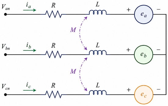
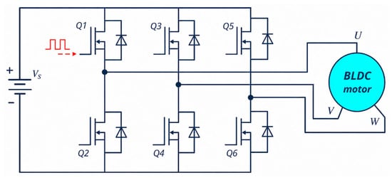
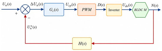
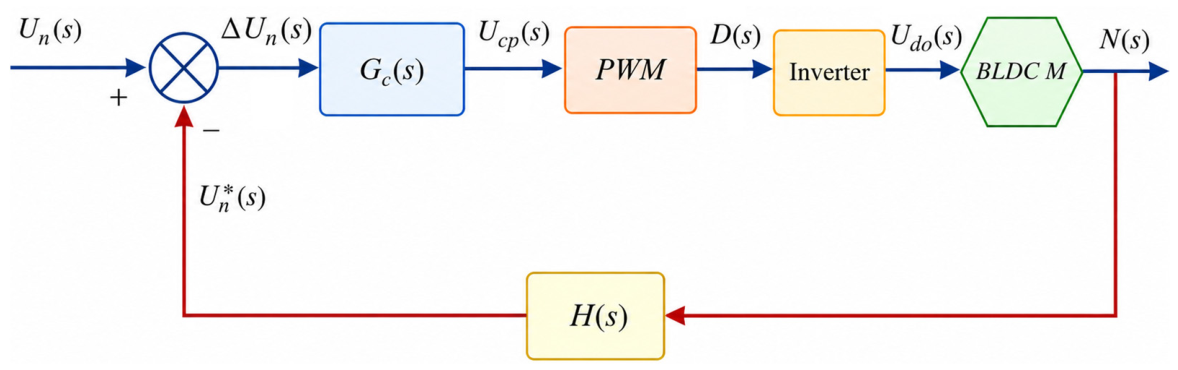
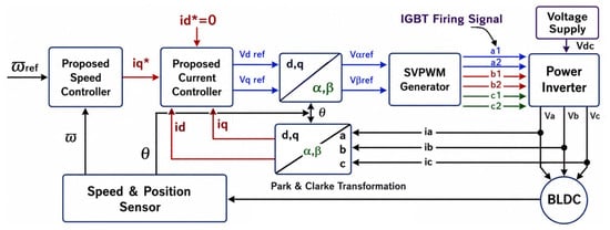
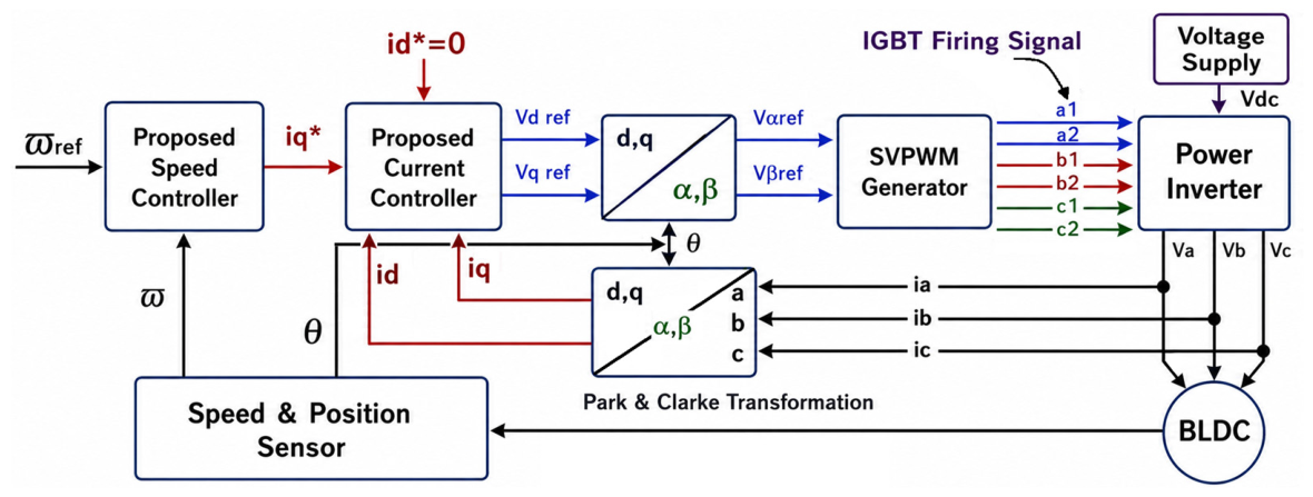
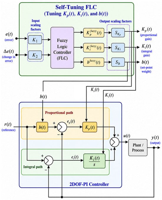
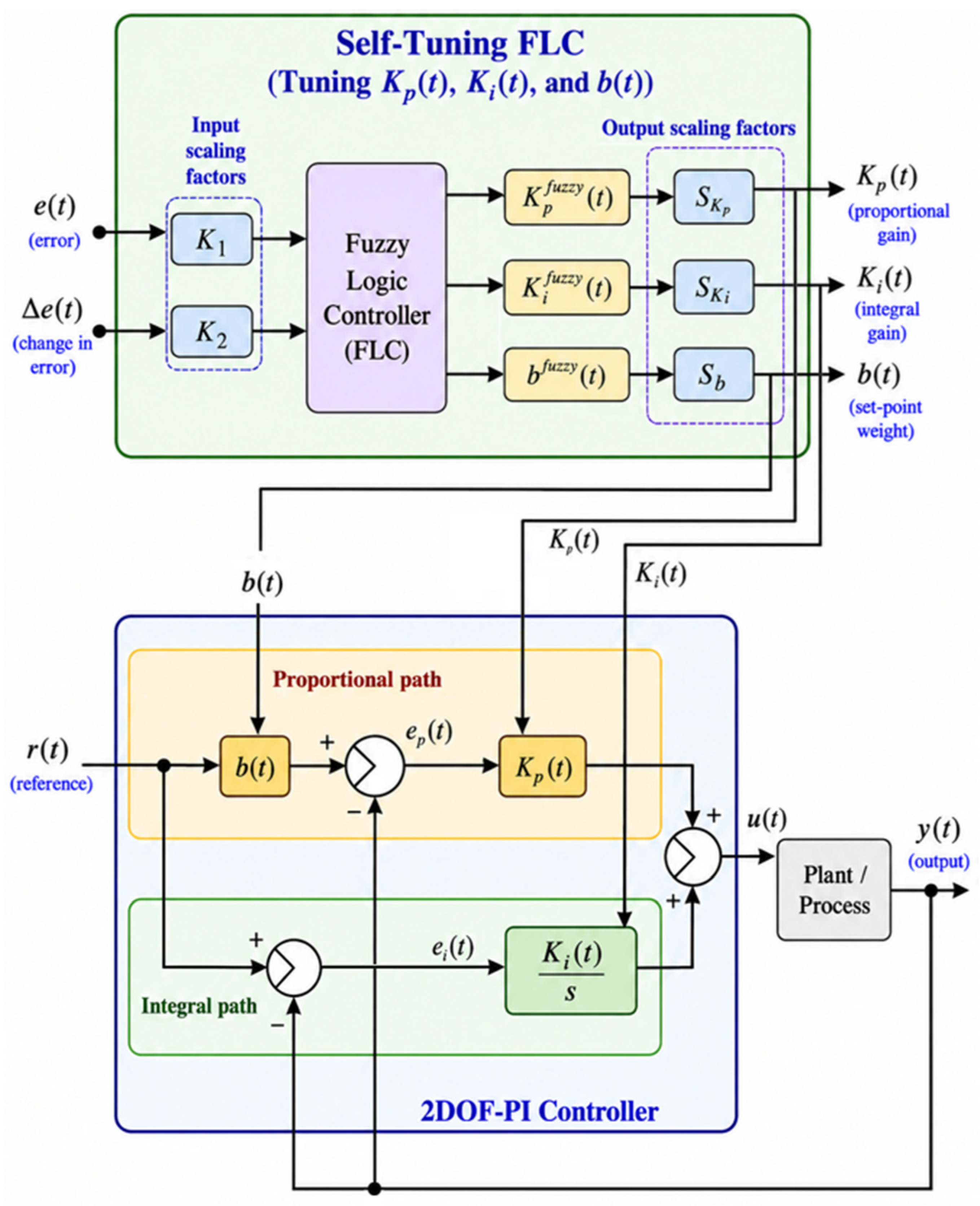
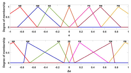
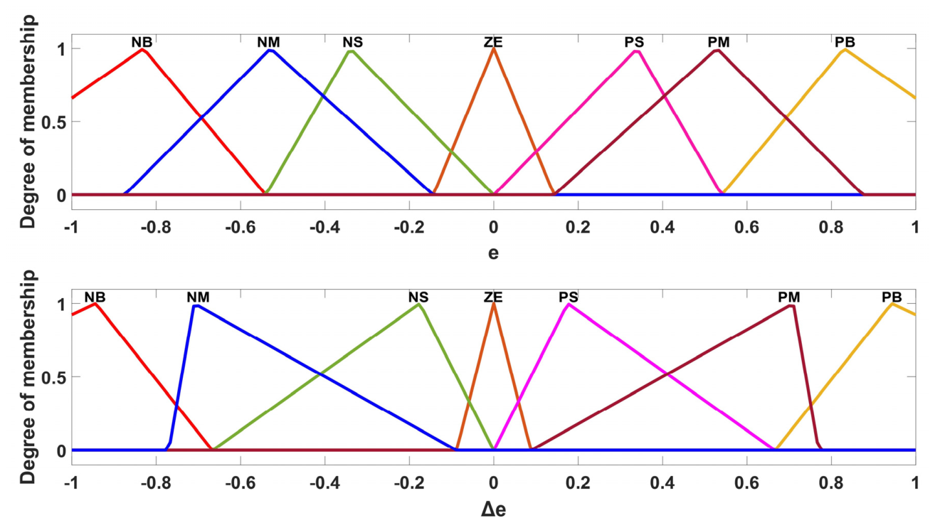
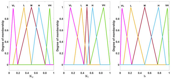
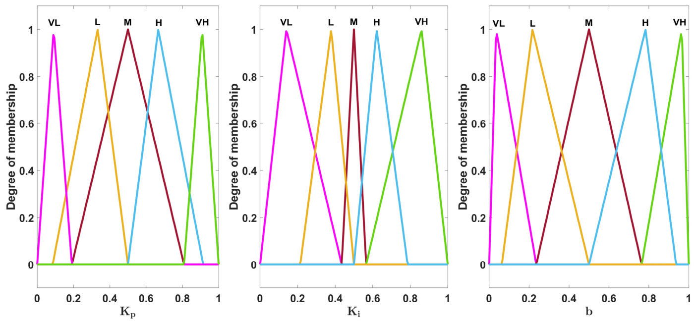
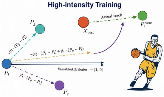
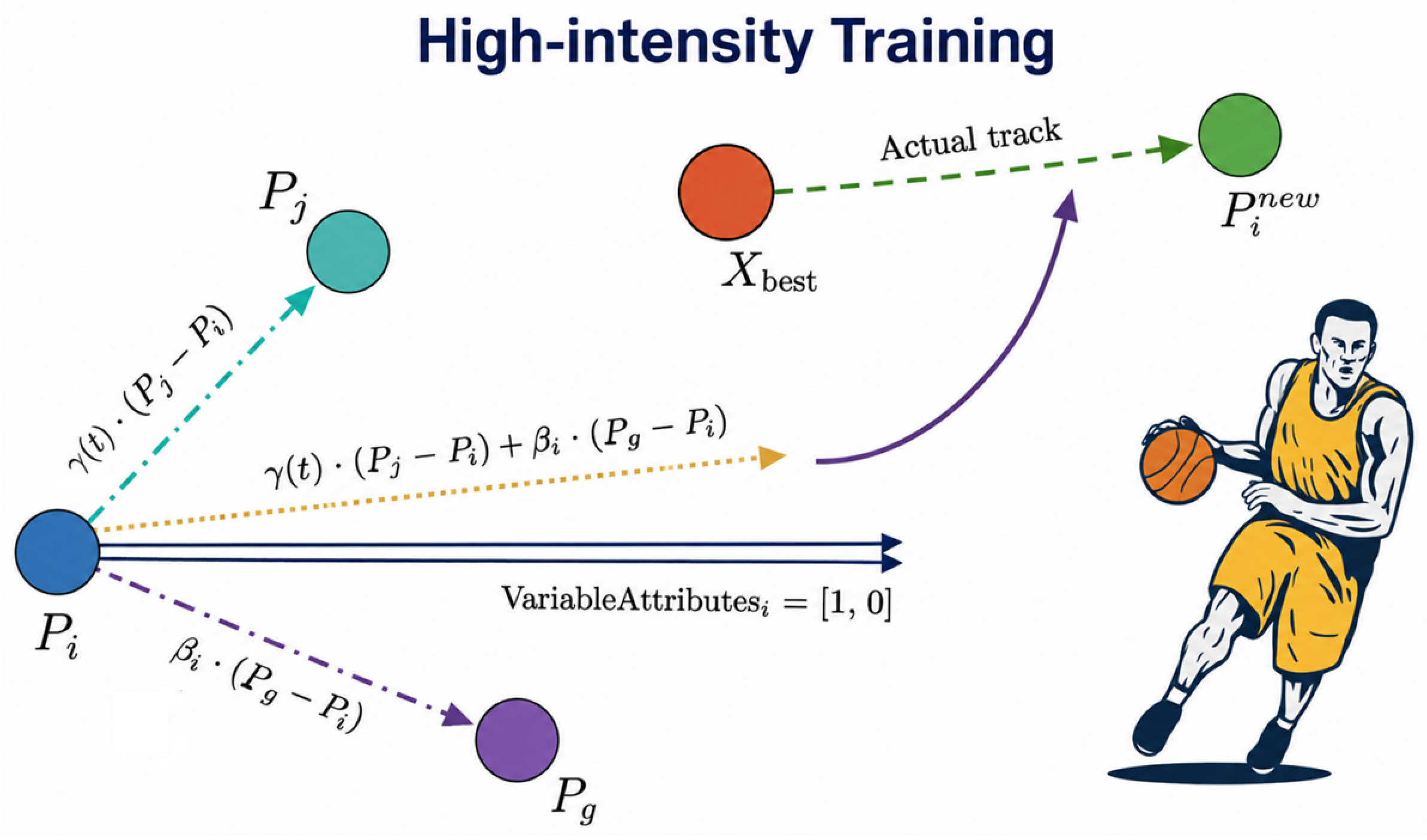
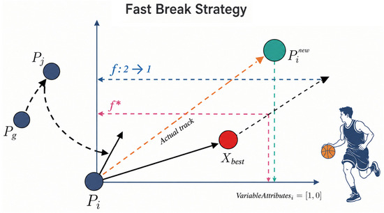
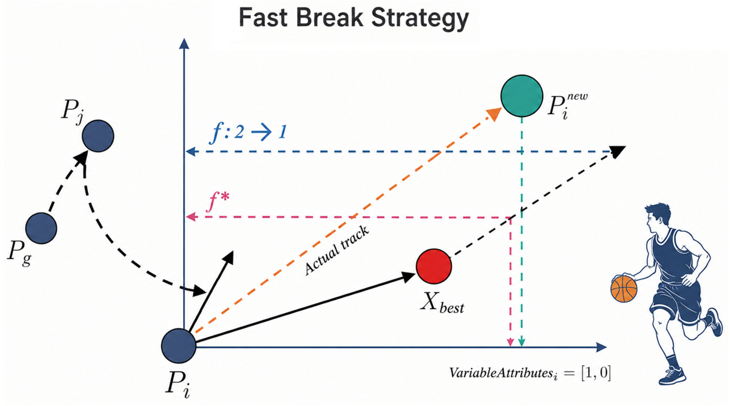
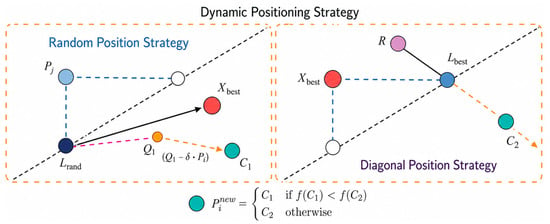
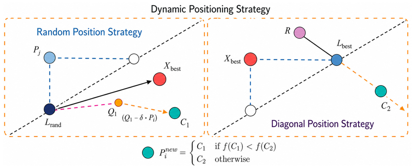
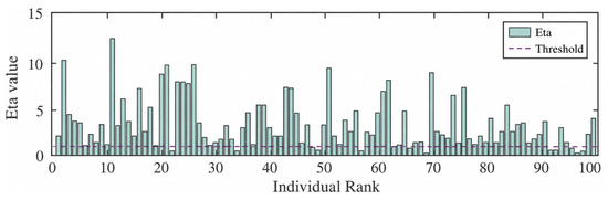
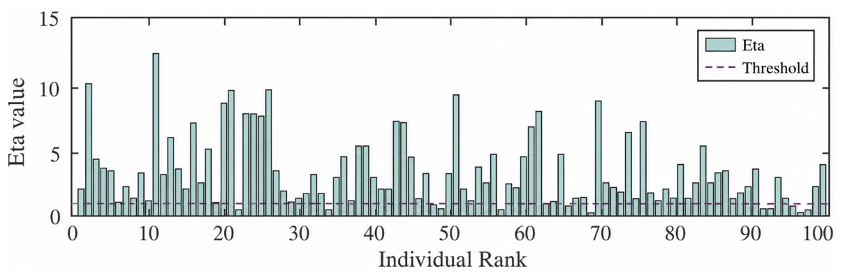
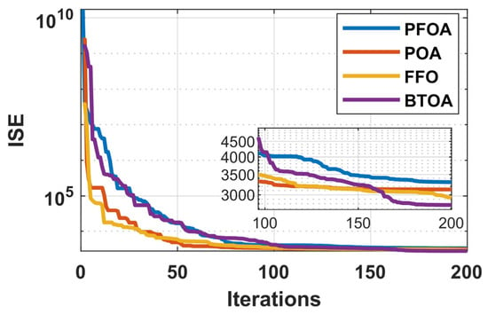
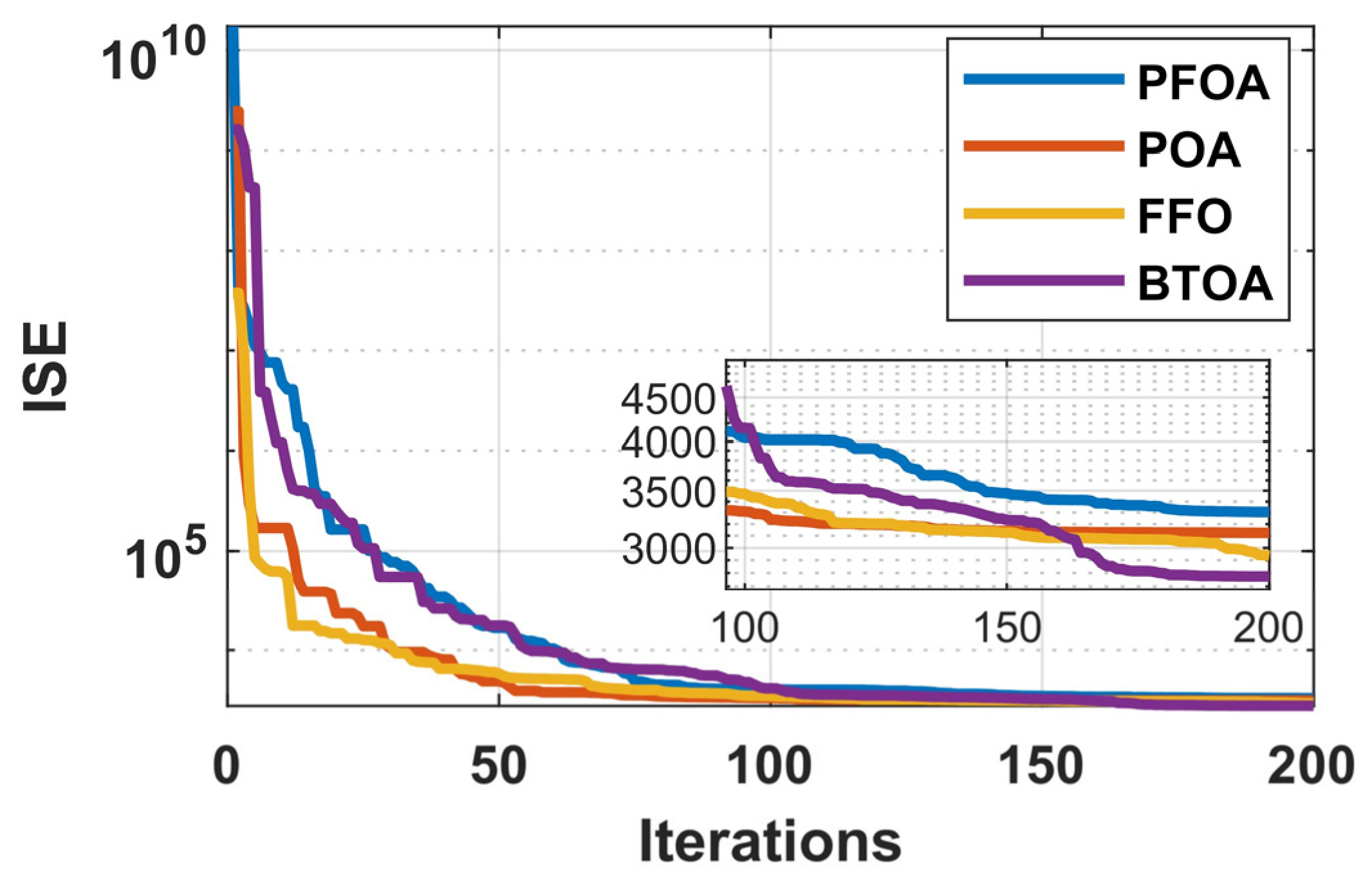
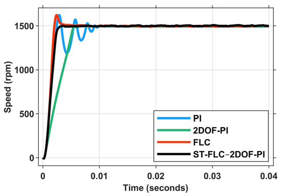
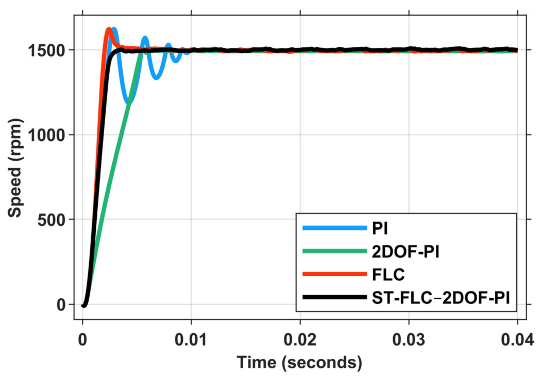
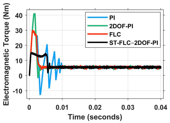
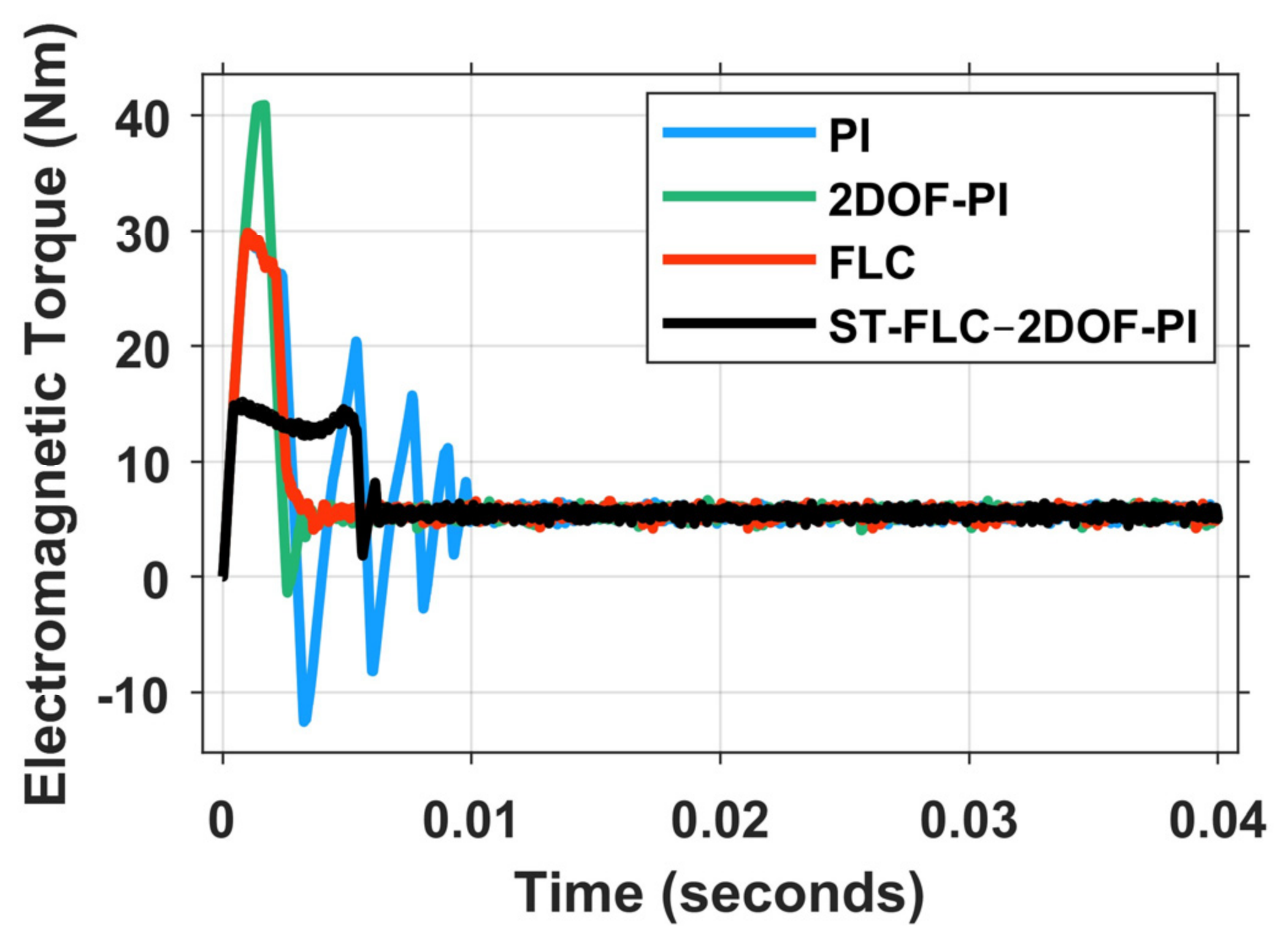
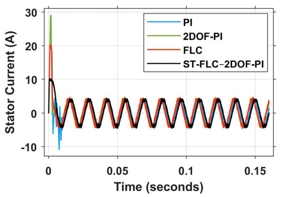
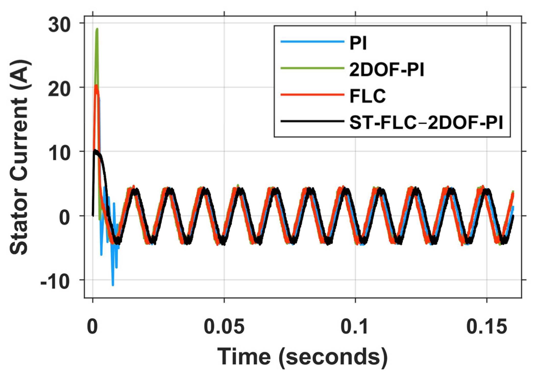
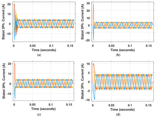
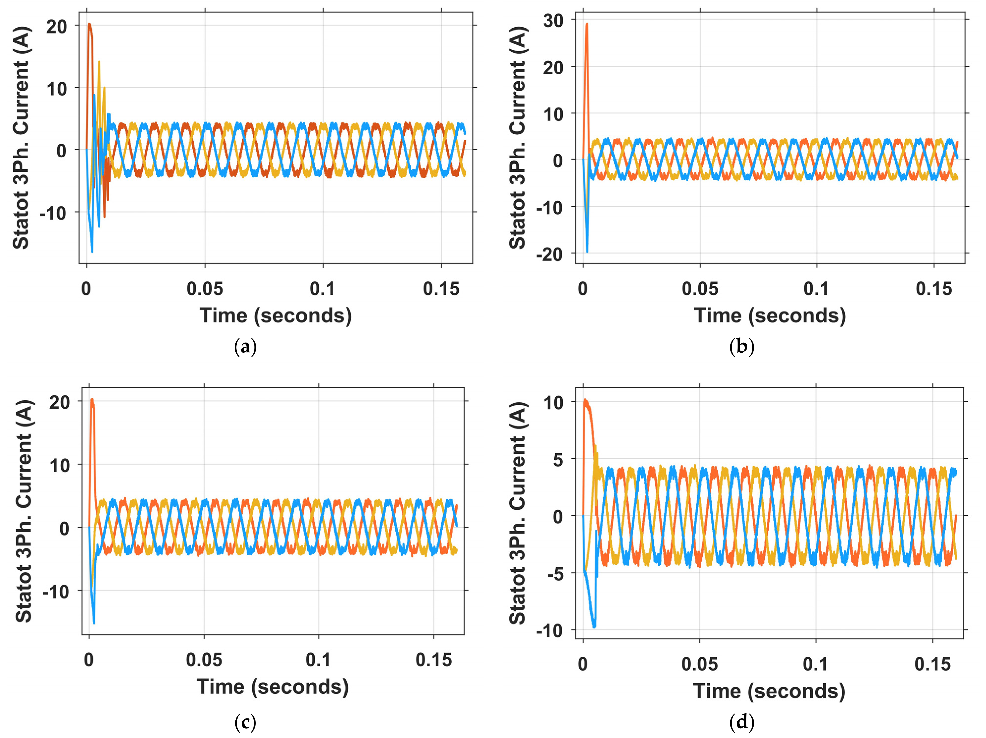
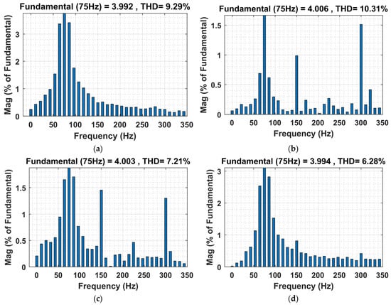
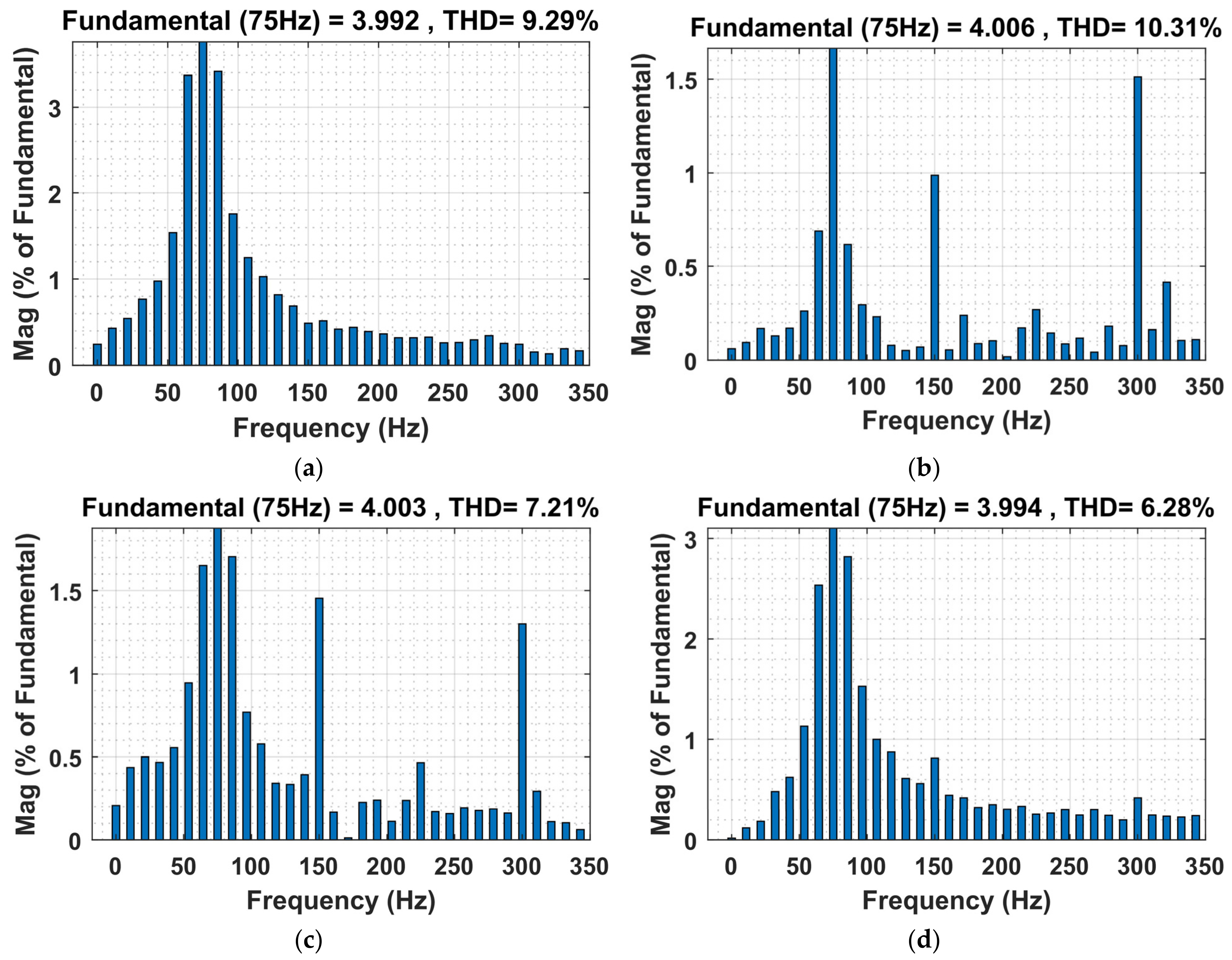
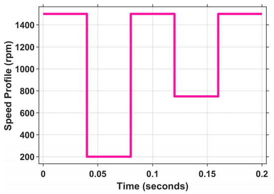
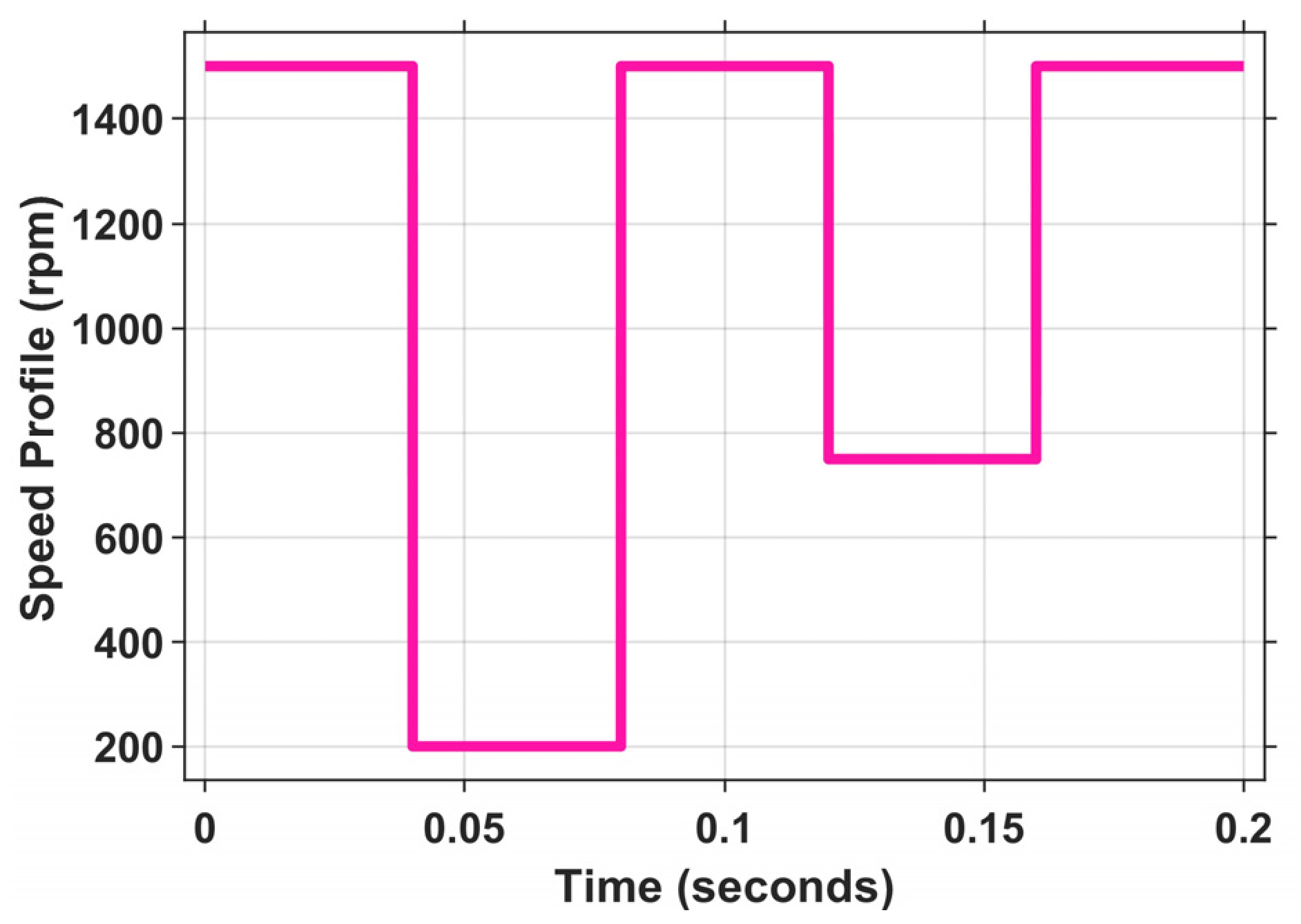
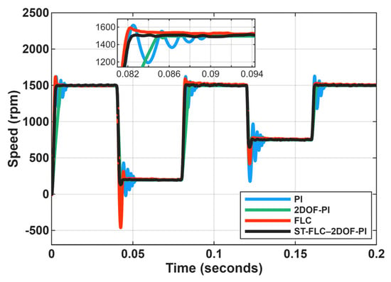
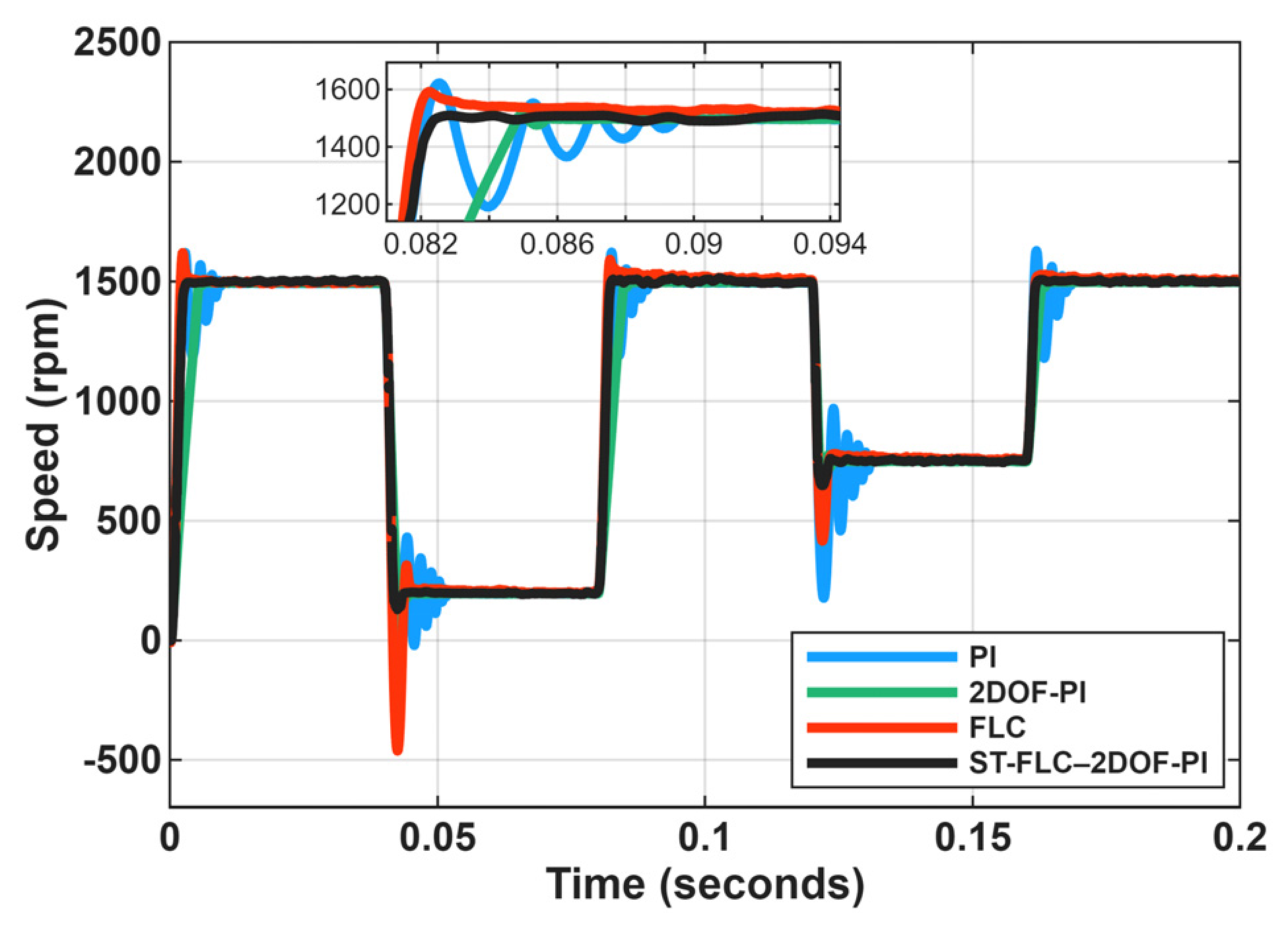
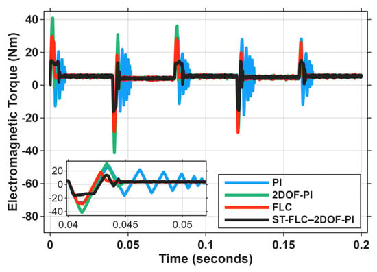
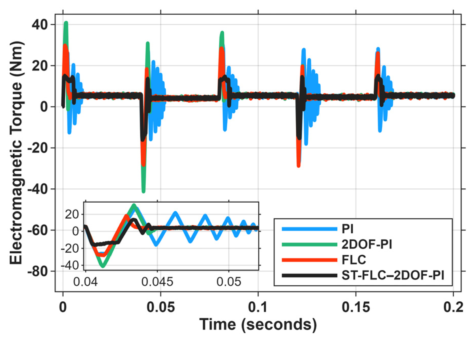
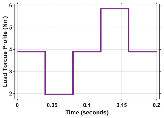
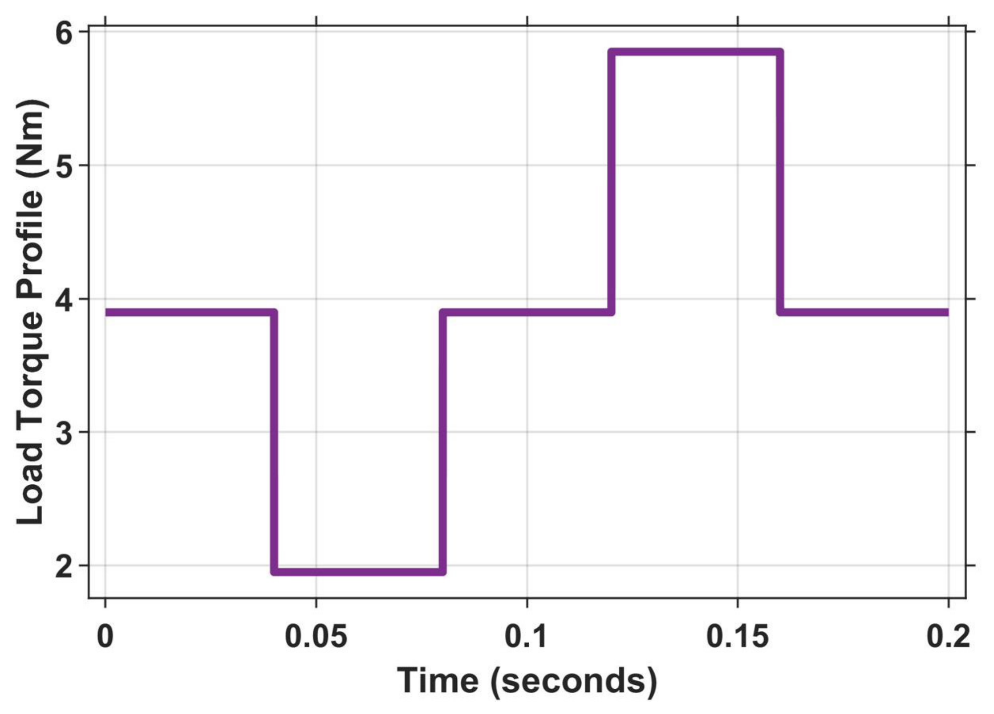
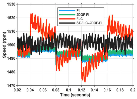
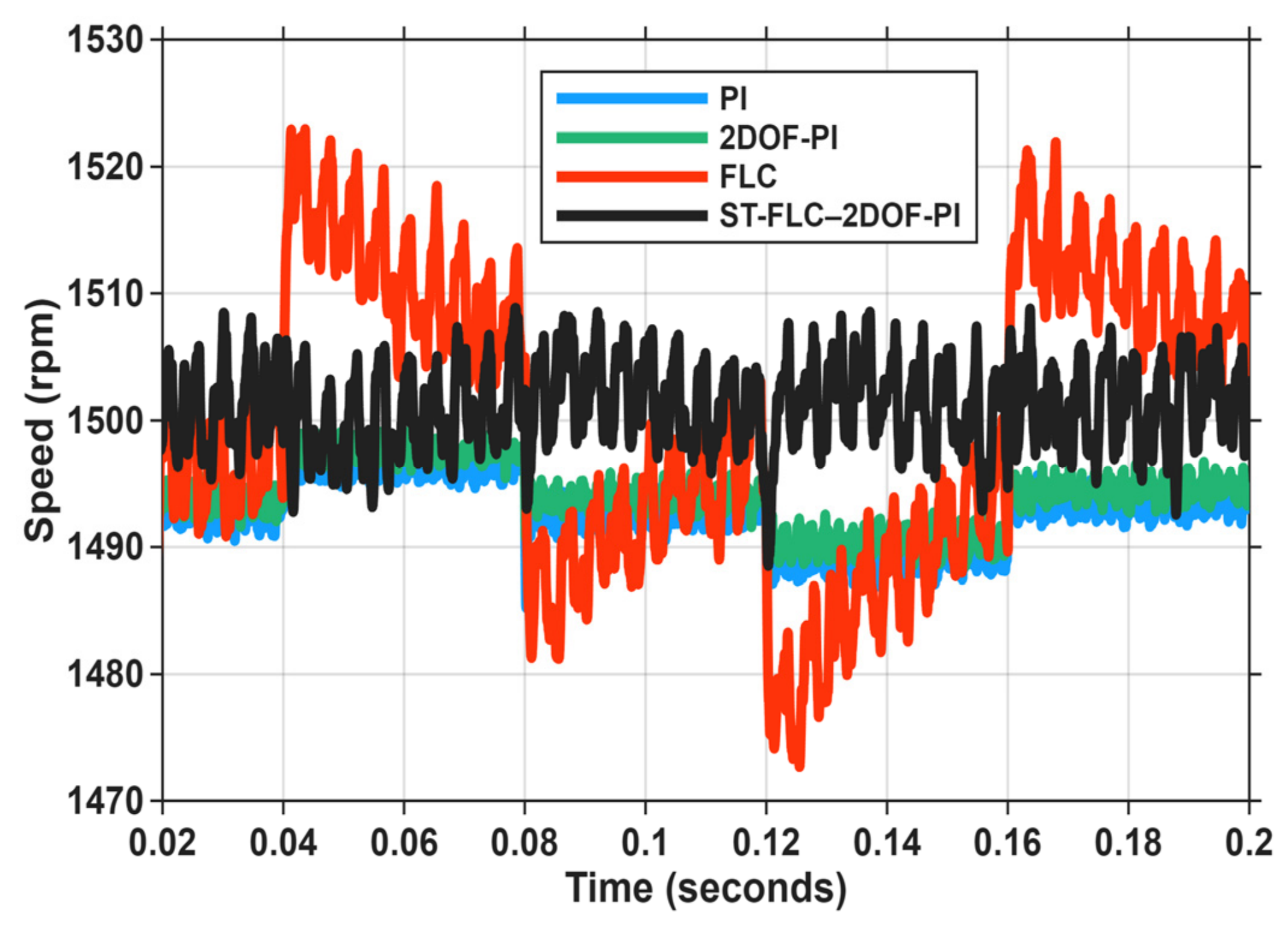
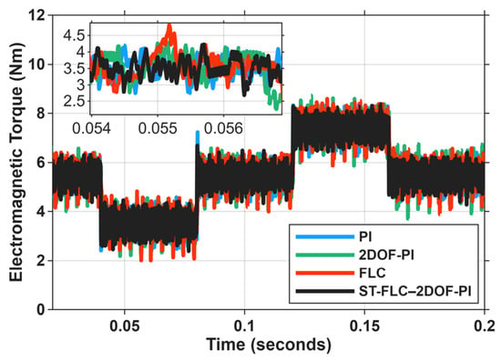
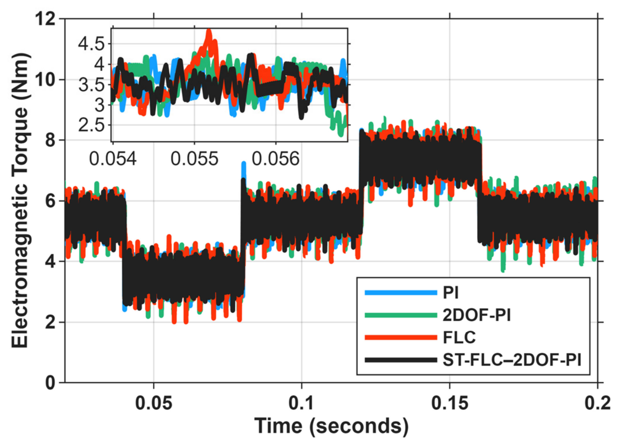
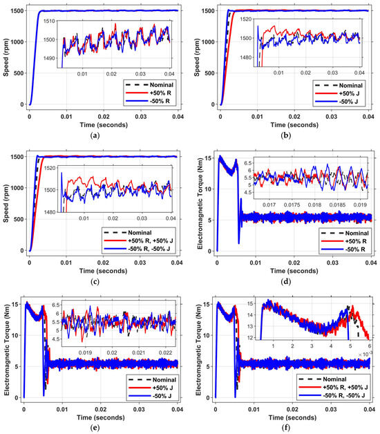
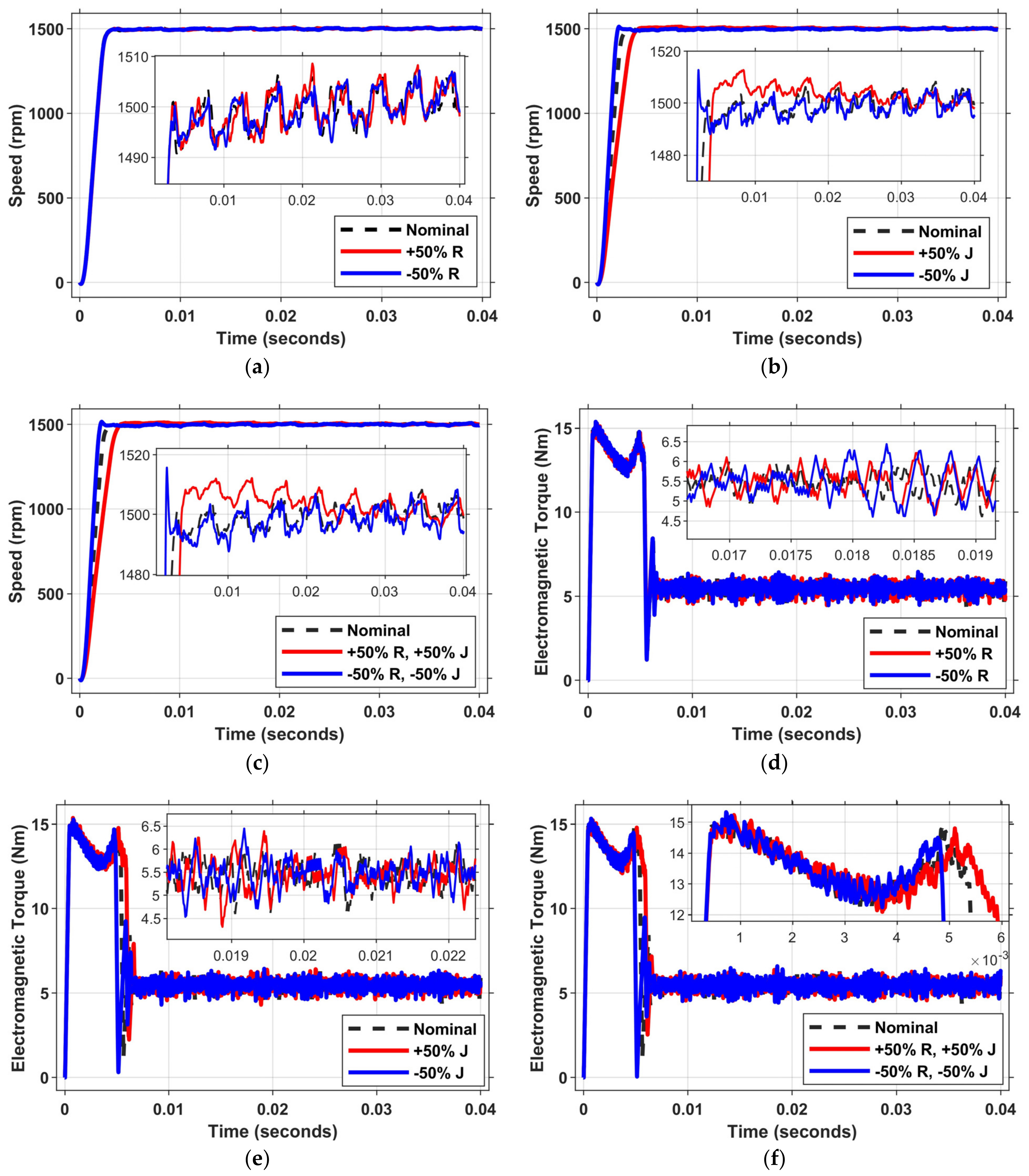
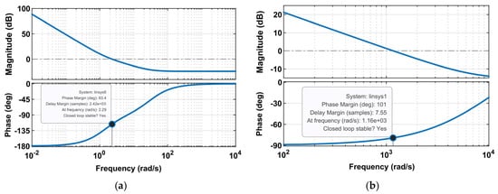
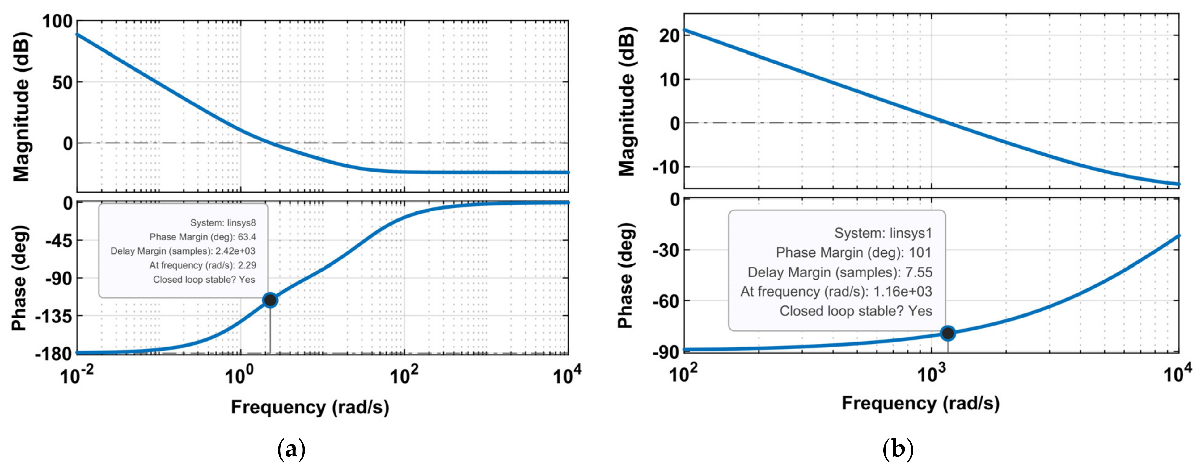
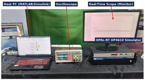
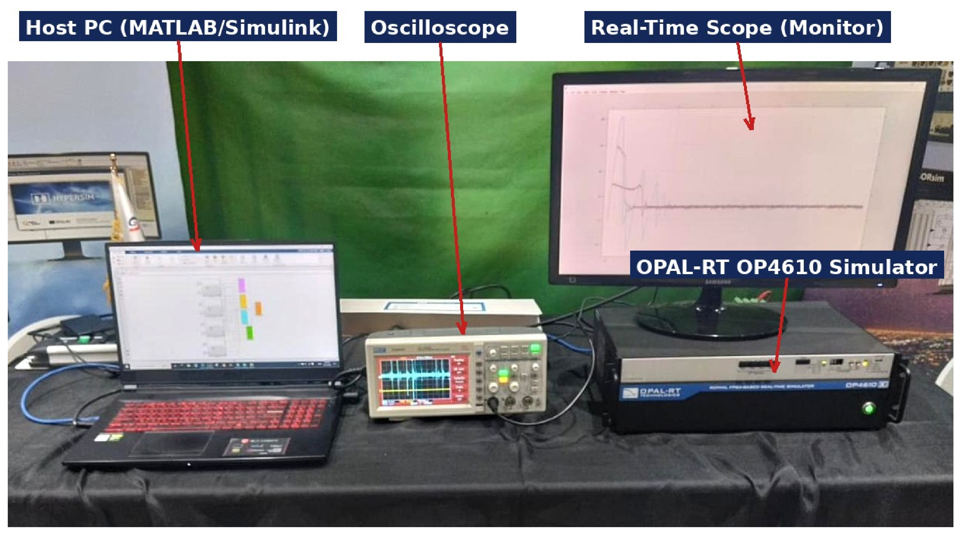
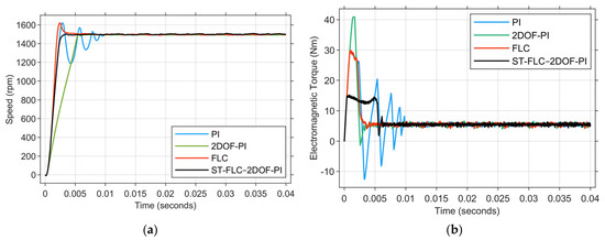
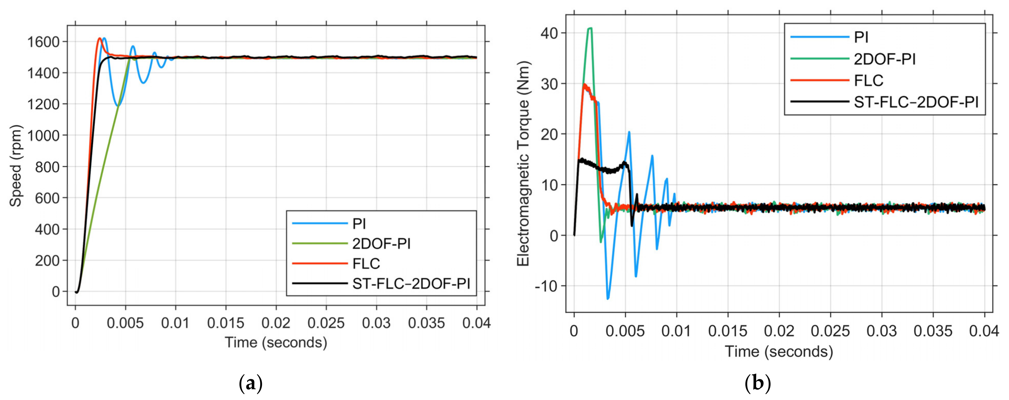

Disclaimer/Publisher’s Note: The statements, opinions and data contained in all publications are solely those of the individual author(s) and contributor(s) and not of MDPI and/or the editor(s). MDPI and/or the editor(s) disclaim responsibility for any injury to people or property resulting from any ideas, methods, instructions or products referred to in the content. |
© 2026 by the authors. Licensee MDPI, Basel, Switzerland. This article is an open access article distributed under the terms and conditions of the Creative Commons Attribution (CC BY) license.