Permutation Contractions in Complete b-Metric Spaces: Fixed Point Results and Applications

Abstract

Permutation contractions have recently been investigated as a flexible generalization of classical contractive conditions through suitable combinations of orbit distances. In this paper, we study permutation contractions on a complete b-metric space and establish a generalized Banach-type fixed point theorem ensuring the existence and uniqueness of a fixed point. We further derive a per-term dominated version in which each orbital distance is controlled by the base distance, leading to a global contractive condition and a corresponding fixed point theorem. As a consequence, suitable Kannan- and restricted Hardy–Rogers-type fixed point results are obtained under additional assumptions. To illustrate the applicability of the theoretical results, we apply the obtained fixed point principles to prove the existence and uniqueness of solutions of a linear system of equations and to the existence of a solution for a second-order boundary value problem. These results demonstrate that permutation contractions provide a flexible framework for extending fixed point techniques in b-metric spaces.

1. Introduction and Preliminaries

Fixed point (FP) theory provides a fundamental framework for the analysis of nonlinear problems arising in analysis, differential equations [1,2], integral equations [3,4], and applied mathematics. The classical Banach contraction principle [5] is one of the central results in this area, establishing the existence and uniqueness of an FP for a contraction on a complete metric space. Since its introduction, numerous generalizations have been developed by modifying either the underlying space or the contractive condition. In particular, Kannan-type contractions [6,7,8] and Chatterjea-type contractions [9] have provided important extensions of the classical Banach principle by incorporating different combinations of distances. These developments show that the choice of the distances appearing in a contractive condition can substantially enlarge the class of mappings for which FP results remain valid.

In parallel with these developments, the classical metric framework has been extended in numerous directions to accommodate more flexible notions of distance and to broaden the scope of FP theory. Among the early developments, Branciari introduced rectangular metric spaces [10,11] by replacing the classical triangle inequality with a four-point inequality, while Matthews [12,13] proposed partial metric spaces in which the self-distance of a point need not vanish. Further generalizations include quasi-metric spaces, cone metric spaces and dislocated metric spaces, each providing a distinct modification of the underlying metric structure while preserving suitable properties for convergence and FP analysis. In this continuing development, b-metric spaces, introduced by Czerwik in [14], have emerged as a particularly useful and widely studied framework in which the standard triangle inequality is relaxed by means of a constant $b\ge 1$. The triangle inequality makes the b-metric spaces particularly suitable for studying nonlinear operators for which the standard metric framework is too restrictive [15,16]. FP principles in these spaces provide useful tools for treating a broad range of nonlinear problems. Let us recall the definition of a b-metric space.

Definition 1.

Let Υ be a nonempty set and $b\ge 1$. A b-metric is a function $\underline{\mathcal{B}}:\mathrm{Y}\times \mathrm{Y}\to [0,\infty )$ such that for all $a_1,a_2,a_3\in \mathrm{Y}$,

1.

$\underline{\mathcal{B}}(a_1,a_2)=0⟺a_1=a_2$;

2.

$\underline{\mathcal{B}}(a_1,a_2)=\underline{\mathcal{B}}(a_2,a_1)$;

3.

$\underline{\mathcal{B}}(a_1,a_2)\le b[\underline{\mathcal{B}}(a_1,a_3)+\underline{\mathcal{B}}(a_3,a_2)]$.

From this perspective, the generalization of the underlying distance structure is closely connected with the broader question of which metric quantities should enter a contractive condition. Classical contraction schemes typically involve only a finite collection of distances associated with two points and their first images. A more flexible approach is obtained by considering distances along the entire orbit of the mapping. For a self-map $\mathcal{F}:\mathrm{Y}\to \mathrm{Y}$, this leads naturally to the family of $(p,q)$-orbit distances ${\underline{\mathcal{B}}}_{p,q}(e,h)=\underline{\mathcal{B}}({\mathcal{F}}^{p}e,{\mathcal{F}}^{q}h),p,q\in \mathbb{N}.$ Such a formulation simultaneously encompasses the distance between the original points, the distance between their images, mixed point–image distances, and displacement terms of the form $\left(\underline{\mathcal{B}}(e,\mathcal{F}e)\right)$ and $\left(\underline{\mathcal{B}}(h,\mathcal{F}h)\right)$. It therefore provides a natural mechanism for placing various classical contraction conditions within a common orbit-based framework.

Recently, Ayoob and Mlaiki [17] developed a permutation contraction framework in which the contractive condition involves an infinite weighted collection of orbital distances $\underline{\mathcal{B}}({\mathcal{F}}^{p}x,{\mathcal{F}}^{q}y)$ with the terms arranged according to an arbitrary permutation. Their results provide a unified formulation encompassing several classical contraction conditions, including some contractions, and establish corresponding FP results in a complete metric spaces. This framework contains many familiar contraction schemes as special cases while allowing interactions between arbitrarily high iterates of the mapping. In particular, it provides a unified setting in which the structure of the contractive condition is determined not only by the mapping itself but also by the selection, weighting, and permutation of orbit distances. The following definition introduce the orbit and orbit distances needed next to define the permutation contraction.

Definition 2

([17]). Let $(\mathrm{Y},\underline{\mathcal{B}})$ be a metric space and let $\mathcal{F}:\mathrm{Y}\to \mathrm{Y}$ be a self-map. For any $u\in \mathrm{Y}$, the (forward) orbit of u under $\mathcal{F}$ is defined by

$$O\left(u\right)=\{{\mathcal{F}}^{n}u:n\in \mathbb{N}\}.$$

For a pair $(u,v)\in \mathrm{Y}\times \mathrm{Y}$ and integers $p,q\in \mathbb{N}$, the $(p,q)$-orbit distance is defined by

$${\underline{\mathcal{B}}}_{p,q}(u,v)=\underline{\mathcal{B}}\left({\mathcal{F}}^{p}u,{\mathcal{F}}^{q}v\right)\in [0,\infty ).$$

To systematically enumerate all such $(p_i,q_i)$-orbit distances, fix a bijection

$$\iota :\mathbb{N}⟶\mathbb{N}\times \mathbb{N},\iota \left(i\right)=(p_i,q_i),$$

and define the corresponding infinite sequence

$${\underline{\mathcal{B}}}_i(u,v)={\underline{\mathcal{B}}}_{p_i,q_i}(u,v)=\underline{\mathcal{B}}\left({\mathcal{F}}^{p_i}u,{\mathcal{F}}^{q_i}v\right),i\in \mathbb{N}.$$

As particular cases, the metric distances underlying the classical contraction conditions can be recovered as follows.

Remark 1.

Many of the standard contractive conditions encountered in FP theory admit a common description in terms of distances between suitable iterates of the mapping. This observation motivates the introduction of the general distance expression ${\underline{\mathcal{B}}}_{p,q}(u,v)$, from which a number of familiar configurations emerge as special instances. The principal cases are listed below:

$$\begin{array}{ccc}\hfill {\underline{\mathcal{B}}}_{0,0}(u,v)& =\underline{\mathcal{B}}(u,v),\hfill & \hfill (thedistancebetweentheinitialpoints)\\ \hfill {\underline{\mathcal{B}}}_{1,1}(u,v)& =\underline{\mathcal{B}}(\mathcal{F}u,\mathcal{F}v),\hfill & \hfill (thedistancebetweentheirfirstimages)\\ \hfill {\underline{\mathcal{B}}}_{0,1}(u,v)& =\underline{\mathcal{B}}(u,\mathcal{F}v),\hfill & \hfill (amixedpoint–imagedistance)\\ \hfill {\underline{\mathcal{B}}}_{1,0}(u,v)& =\underline{\mathcal{B}}(\mathcal{F}u,v),\hfill & \hfill (thecomplementarymixedistance)\\ \hfill {\underline{\mathcal{B}}}_{0,1}(u,u)& =\underline{\mathcal{B}}(u,\mathcal{F}u),\hfill & \hfill (self\text{-}distanceofuunder\mathcal{F})\\ \hfill {\underline{\mathcal{B}}}_{0,1}(v,v)& =\underline{\mathcal{B}}(v,\mathcal{F}v),\hfill & \hfill (self\text{-}distanceofvunder\mathcal{F})\end{array}$$

Severals contraction schemes can be formulated through suitable combinations of these six fundamental distances.

The permutation contraction is defined as follows:

Definition 3

([17]). Let $(\mathrm{Y},\underline{\mathcal{B}})$ be a metric space and $\mathcal{F}:\mathrm{Y}\to \mathrm{Y}$ a self-map. Fix a permutation $\tau :\mathbb{N}\to \mathbb{N}$ and a sequence of non-negative real numbers ${\left(c_i\right)}_{i\ge 1}$ such that

$$\Lambda ={\displaystyle \sum _{i=1}^{\infty }}{c}_i<1.$$

Then, $\mathcal{F}$ is said to be a permutation contraction if for all $u,v\in \mathrm{Y}$,

$$\underline{\mathcal{B}}(\mathcal{F}u,\mathcal{F}v)\le {\displaystyle \sum _{i=1}^{\infty }}{c}_i{\underline{\mathcal{B}}}_{\tau \left(i\right)}(u,v),$$

where each ${\underline{\mathcal{B}}}_{\tau \left(i\right)}(u,v)$ denotes the $(p_{\tau \left(i\right)},q_{\tau \left(i\right)})$-orbit distance

$${\underline{\mathcal{B}}}_{\tau \left(i\right)}(u,v)=\underline{\mathcal{B}}\left({\mathcal{F}}^{p_{\tau \left(i\right)}}u,{\mathcal{F}}^{q_{\tau \left(i\right)}}v\right),$$

with $(p_j,q_j)$ representing the enumeration of $\mathbb{N}\times \mathbb{N}$.

Concerning the convergence of the infinite series, since the non-negative coefficients ${\left(c_i\right)}_{i\ge 1}$ are summable, with $\Lambda ={\sum }_{i=1}^{\infty }{c}_i<1$, the infinite weighted sum in the contractive condition is well defined whenever the associated orbital distances are uniformly bounded. This requirement is fulfilled, in particular, if the Picard orbit $\left\{u^{\left(n\right)}\right\}$ is bounded.

Remark 2.

The permutation contraction introduced above provides a unified framework encompassing a variety of classical contractive mappings. Appropriate choices of the weights $\left(c_i\right)$ and the permutation τ recover several familiar contraction conditions, including the following fundamental cases:

• Banach contraction: Choose $c_1=k$ with $0\le k<1$, and $c_i=0$ for $i\ge 2$, together with ${\underline{\mathcal{B}}}_{\tau \left(1\right)}(u,v)=\underline{\mathcal{B}}(u,v)$. Then, the inequality reduces to

  $$\underline{\mathcal{B}}(\mathcal{F}u,\mathcal{F}v)\le k\underline{\mathcal{B}}(u,v).$$
• Kannan contraction: Choose $c_1=c_2=k$ with $0\le k<\frac{1}{2}$, and $c_i=0$ for $i\ge 3$, with ${\underline{\mathcal{B}}}_{\tau \left(1\right)}(u,v)=\underline{\mathcal{B}}(u,\mathcal{F}u)$ and ${\underline{\mathcal{B}}}_{\tau \left(2\right)}(u,v)=\underline{\mathcal{B}}(v,\mathcal{F}v)$. Then,

  $$\underline{\mathcal{B}}(\mathcal{F}u,\mathcal{F}v)\le k\left(\underline{\mathcal{B}}(u,\mathcal{F}u)+\underline{\mathcal{B}}(v,\mathcal{F}v)\right).$$

Despite the elegance of the permutation contraction framework proposed by Ayoob and Mlaiki [17], its development and related FP theorems have so far been limited to standard metric spaces. In these spaces, the usual triangle inequality is always true. On the hand, FP theory in b-metric spaces [14,15,16] has been well developed to deal with nonlinear operators under more flexible geometric conditions. However, the existing research does not have a way to extend infinite orbital permutation contractions to spaces that have a parameter $b\ge 1$. Also, the way the structural parameter b interacts with weighted series of orbit distances has not been studied at all. This includes how relaxed triangle conditions affect the convergence rules of Kannan-type estimates and how operators can be used in value problems.

To fill this gap, in this paper, we take the permutation contraction framework and apply it to complete b-metric spaces. We show that there is an FP for infinite weighted permutation contractions under b-metric limits. We also create Kannan- and Hardy–Rogers-type conditions as specific examples. Finally, we show how these ideas work in situations like second-order boundary value problems and linear systems.

The remainder of the paper is organized as follows. Section 2 contains the main FP results for permutation contractions on a complete b-metric space ($C-\mathcal{B}m$), including the per-term dominated case. We also obtain Kannan- and restricted Hardy–Rogers-type results as special cases. Section 3 presents applications to a linear system of equations and a second-order boundary value problem to highlight the versatility of permutation contractions in b-metric spaces. Finally, Section 4 concludes the paper and outlines possible directions for further research.

2. Main Results

2.1. Fixed Point Result for Permutation-Based Contractions

We first establish the main FP theorem for permutation contractions on a $C-\mathcal{B}m$. The result provides sufficient conditions, expressed through the weighted orbit-distance, that ensure the convergence of the associated Picard iteration and, consequently, the existence and uniqueness of an FP.

Theorem 1.

Let $(\mathrm{Y},\underline{\mathcal{B}})$ be a $C-\mathcal{B}m$ and let $\mathcal{F}:\mathrm{Y}\to \mathrm{Y}$ be a permutation contraction in the sense that

$$\underline{\mathcal{B}}(\mathcal{F}u,\mathcal{F}v)\le {\displaystyle \sum _{i=1}^{\infty }}{c}_i{\underline{\mathcal{B}}}_{\tau \left(i\right)}(u,v),{\underline{\mathcal{B}}}_{p,q}(u,v)=\underline{\mathcal{B}}({\mathcal{F}}^{p}u,{\mathcal{F}}^{q}v),$$

(1)

for some non-negative weights ${\left(c_i\right)}_{i\ge 1}$ with ${\displaystyle \Lambda ={\displaystyle \sum _{i=1}^{\infty }}{c}_i<\infty }$ and a permutation $\tau :\mathbb{N}\to \mathbb{N}$ of a fixed enumeration ${\left\{(p_i,q_i)\right\}}_{i\ge 1}$ of $\mathbb{N}\times \mathbb{N}$. Assume there exist non-negative numbers ${\left\{{\delta }_i\right\}}_{i\ge 1}$ and ${\left\{{\Delta }_i\right\}}_{i\ge 1}$ such that for every $z\in \mathrm{Y}$ and every $n\ge 1$, one has the bound

$$\underline{\mathcal{B}}\left({\mathcal{F}}^{n+p_i}z,{\mathcal{F}}^{n-1+q_i}z\right)\le {\delta }_i\underline{\mathcal{B}}\left({\mathcal{F}}^{n}z,{\mathcal{F}}^{n-1}z\right)+{\Delta }_i\underline{\mathcal{B}}\left({\mathcal{F}}^{n+1}z,{\mathcal{F}}^{n}z\right),\forall i\in \mathbb{N}.$$

(2)

Set

$$M_1={\displaystyle \sum _{i=1}^{\infty }}{c}_i{\delta }_i,M_2={\displaystyle \sum _{i=1}^{\infty }}{c}_i{\Delta }_i.$$

(3)

Suppose

$$M_2<1,b{M}_1+M_2<1and\Lambda >{\displaystyle \frac{1}{b^3}}-{\displaystyle \frac{M_1}{1-M_2}}.$$

(4)

Then, $\mathcal{F}$ has a unique fixed point $s\in \mathrm{Y}$.

Proof. 

Fix $u^{\left(0\right)}\in \mathrm{Y}$ and define $u^{\left(n\right)}={\mathcal{F}}^n{u}^{\left(0\right)}$ and ${\mathcal{B}}_n=\underline{\mathcal{B}}(u^{(n+1)},u^{\left(n\right)})$ for $n\ge 0$. Applying (1) to the pair $(u^{\left(n\right)},u^{(n-1)})$ and using ${\underline{\mathcal{B}}}_{p,q}(u^{\left(n\right)},u^{(n-1)})=\underline{\mathcal{B}}({\mathcal{F}}^{n+p}{u}^{\left(0\right)},{\mathcal{F}}^{n-1+q}{u}^{\left(0\right)})$ yields

$${\mathcal{B}}_n=\underline{\mathcal{B}}(u^{(n+1)},u^{\left(n\right)})\le {\displaystyle \sum _{i=1}^{\infty }}{c}_i\underline{\mathcal{B}}\left({\mathcal{F}}^{n+p_i}{u}^{\left(0\right)},{\mathcal{F}}^{n-1+q_i}{u}^{\left(0\right)}\right),n\ge 1.$$

(5)

By (2) with $z=u^{\left(0\right)}$, we have, termwise in the sum,

$$\underline{\mathcal{B}}\left({\mathcal{F}}^{n+p_i}{u}^{\left(0\right)},{\mathcal{F}}^{n-1+q_i}{u}^{\left(0\right)}\right)\le {\delta }_i{\mathcal{B}}_{n-1}+{\Delta }_i{\mathcal{B}}_n,n\ge 1.$$

(6)

Upon applying (5) and (6), we deduce that

$${\mathcal{B}}_n\le \left({\displaystyle \sum _{i=1}^{\infty }}{c}_i{\delta }_i\right){\mathcal{B}}_{n-1}+\left({\displaystyle \sum _{i=1}^{\infty }}{c}_i{\Delta }_i\right){\mathcal{B}}_n=M_1{\mathcal{B}}_{n-1}+M_2{\mathcal{B}}_n.$$

(7)

Since $M_2<1$, inequality (7) may be rewritten as

$$(1-M_2){\mathcal{B}}_n\le M_1{\mathcal{B}}_{n-1}⟹{\mathcal{B}}_n\le \alpha {\mathcal{B}}_{n-1},\alpha ={\displaystyle \frac{M_1}{1-M_2}}\in [0,1).$$

(8)

Applying (8) successively, we obtain

$${\mathcal{B}}_n\le {\alpha }^n{\mathcal{B}}_0={\alpha }^n\underline{\mathcal{B}}(u^{\left(1\right)},u^{\left(0\right)}),n\ge 0.$$

(9)

From (9) and using the triangle inequality for $m>n$, we obtain

$$\begin{array}{ccc}\hfill \underline{\mathcal{B}}(u^{\left(m\right)},u^{\left(n\right)})\le {\displaystyle \sum _{k=n}^{m-1}}{b}^{k-n+1}{\mathcal{B}}_k& \le & {\mathcal{B}}_0{b}^{1-n}{\displaystyle \sum _{k=n}^{m-1}}{\left(b\alpha \right)}^k\hfill \\ & \le & {\mathcal{B}}_0{b}^{1-n}{\displaystyle \sum _{k=n}^{\infty }}{\left(b\alpha \right)}^k\hfill \\ & \le & b^{1-n}\underline{\mathcal{B}}(u^{\left(1\right)},u^{\left(0\right)}){\displaystyle \frac{{\left(b\alpha \right)}^n}{1-b\alpha }}\hfill \end{array}$$

(10)

Since $b\ge 1$ and using condition (4), then $b^{1-n}\le 1$ and $b\alpha <1$. It follows that $\left\{u^{\left(n\right)}\right\}$ is a Cauchy sequence; since $\mathrm{Y}$ is complete, there exists $s\in \mathrm{Y}$ such that $u^{\left(n\right)}\to s$.

We next verify that s is an FP. Since $u^{(n+1)}=\mathcal{F}{u}^{\left(n\right)}$ and the metric is continuous, passing to the limit as $n\to \infty$ gives

$$\underline{\mathcal{B}}(\mathcal{F}s,s)\le b[\underline{\mathcal{B}}(\mathcal{F}s,u^{(n+1)})+\underline{\mathcal{B}}(u^{(n+1)},s)]⟶b\underset{n\to \infty }{lim\; sup}\underline{\mathcal{B}}(\mathcal{F}s,u^{(n+1)}).$$

(11)

Applying (1) to the pair $(s,u^{\left(n\right)})$ gives

$$\underline{\mathcal{B}}(\mathcal{F}s,u^{(n+1)})=\underline{\mathcal{B}}(\mathcal{F}s,\mathcal{F}{u}^{\left(n\right)})\le {\displaystyle \sum _{i=1}^{\infty }}{c}_i\underline{\mathcal{B}}\left({\mathcal{F}}^{p_i}s,{\mathcal{F}}^{q_i}{u}^{\left(n\right)}\right).$$

(12)

Fixing i, the finiteness of $q_i\in \mathbb{N}$ and the convergence $u^{\left(n\right)}\to s$ ensure that ${\mathcal{F}}^{q_i}{u}^{\left(n\right)}\to {\mathcal{F}}^{q_i}s$. Furthermore, combining the triangle inequality with the geometric estimate in (9), we deduce that

$$\underline{\mathcal{B}}\left({\mathcal{F}}^{p_i}s,{\mathcal{F}}^{q_i}{u}^{\left(n\right)}\right)\le b[\underline{\mathcal{B}}\left({\mathcal{F}}^{p_i}s,{\mathcal{F}}^{q_i}s\right)+\underline{\mathcal{B}}\left({\mathcal{F}}^{q_i}s,{\mathcal{F}}^{q_i}{u}^{\left(n\right)}\right)]\underset{n\to \infty }{\to }b\underline{\mathcal{B}}\left({\mathcal{F}}^{p_i}s,{\mathcal{F}}^{q_i}s\right).$$

(13)

The non-negativity of the series terms allows us to apply Fatou’s lemma; combined with (12) and (13), this yields

$$\underset{n\to \infty }{lim\; sup}\underline{\mathcal{B}}(\mathcal{F}s,u^{(n+1)})\le {\displaystyle \sum _{i=1}^{\infty }}b{c}_i\underline{\mathcal{B}}\left({\mathcal{F}}^{p_i}s,{\mathcal{F}}^{q_i}s\right).$$

(14)

For a fixed i, we apply (2) by setting $z=s$ and $n=1$. Thus, all indices involved in the resulting inequality are non-negative, and we obtain

$$\underline{\mathcal{B}}\left({\mathcal{F}}^{1+p_i}s,{\mathcal{F}}^{q_i}s\right)\le {\delta }_i\underline{\mathcal{B}}(\mathcal{F}s,s)+{\Delta }_i\underline{\mathcal{B}}({\mathcal{F}}^{2}s,\mathcal{F}s).$$

(15)

By the triangle inequality,

$$\underline{\mathcal{B}}\left({\mathcal{F}}^{p_i}s,{\mathcal{F}}^{q_i}s\right)\le b[\underline{\mathcal{B}}\left({\mathcal{F}}^{p_i}s,{\mathcal{F}}^{1+p_i}s\right)+\underline{\mathcal{B}}({\mathcal{F}}^{p_i+1}s,{\mathcal{F}}^{q_i}s)]$$

(16)

Let us prove that $\underline{\mathcal{B}}\left({\mathcal{F}}^{p_i}s,{\mathcal{F}}^{1+p_i}s\right)=\underline{\mathcal{B}}(s,\mathcal{F}s)$.

$$\begin{array}{ccc}\hfill \underline{\mathcal{B}}\left({\mathcal{F}}^{p_i}s,{\mathcal{F}}^{1+p_i}s\right)& =& {\displaystyle \underline{\mathcal{B}}\left({\mathcal{F}}^{p_i}\left(\underset{n\to \infty }{lim}{u}^{\left(n\right)}\right),{\mathcal{F}}^{1+p_i}s\left(\underset{n\to \infty }{lim}{u}^{\left(n\right)}\right)\right)}\hfill \\ & =& {\displaystyle \underline{\mathcal{B}}\left(\underset{n\to \infty }{lim}{\mathcal{F}}^{p_i}\left(u^{\left(n\right)}\right),\underset{n\to \infty }{lim}{\mathcal{F}}^{1+p_i}\left(u^{\left(n\right)}\right)\right)}\hfill \\ & =& {\displaystyle \underline{\mathcal{B}}\left(\underset{n\to \infty }{lim}\left(u^{(n+p_i)}\right),\underset{n\to \infty }{lim}\mathcal{F}\left(u^{(n+p_i)}\right)\right)}\hfill \\ & =& {\displaystyle \underline{\mathcal{B}}\left(\underset{n\to \infty }{lim}{u}^{(n+p_i)},\mathcal{F}\left(\underset{n\to \infty }{lim}{u}^{(n+p_i)}\right)\right)}\hfill \\ & =& \underline{\mathcal{B}}(s,\mathcal{F}s).\hfill \end{array}$$

(17)

Then, from (15), (16) and (17), we obtain

$$\begin{array}{ccc}\hfill \underline{\mathcal{B}}\left({\mathcal{F}}^{p_i}s,{\mathcal{F}}^{q_i}s\right)& \le & b\underline{\mathcal{B}}(s,\mathcal{F}s)+b[{\delta }_i\underline{\mathcal{B}}(\mathcal{F}s,s)+{\Delta }_i\underline{\mathcal{B}}({\mathcal{F}}^{2}s,\mathcal{F}s)]\hfill \\ & \le & b(1+b_i^{-})\underline{\mathcal{B}}(s,\mathcal{F}s)+b{b}_i^{+}\underline{\mathcal{B}}({\mathcal{F}}^{2}s,\mathcal{F}s).\hfill \end{array}$$

(18)

Taking the weighted sum of the inequalities in (18) with respect to the coefficients $c_i$ and then applying (3), we arrive at

$$\begin{array}{ccc}\hfill {\displaystyle \sum _{i=1}^{\infty }}{c}_i\underline{\mathcal{B}}\left({\mathcal{F}}^{p_i}s,{\mathcal{F}}^{q_i}s\right)& \le & {\displaystyle {\displaystyle \sum _{i=1}^{\infty }}b{c}_i(1+b_i^{-})\underline{\mathcal{B}}(\mathcal{F}s,s)+{\displaystyle \sum _{i=1}^{\infty }}b{b}_i^{+}{c}_i\underline{\mathcal{B}}({\mathcal{F}}^{2}s,\mathcal{F}s)}\hfill \\ & \le & b(\Lambda +M_1)\underline{\mathcal{B}}(\mathcal{F}s,s)+b{M}_2\underline{\mathcal{B}}({\mathcal{F}}^{2}s,\mathcal{F}s).\hfill \end{array}$$

(19)

A simultaneous use of (11), (14), and (19), together with (8) applied to the orbit originating at s, yields

$$\begin{array}{ccc}\hfill \underline{\mathcal{B}}(\mathcal{F}s,s)& \le & {\displaystyle b^2{\displaystyle \sum _{i=1}^{\infty }}{c}_i\underline{\mathcal{B}}\left({\mathcal{F}}^{p_i}s,{\mathcal{F}}^{q_i}s\right)}\hfill \\ & \le & b^2[(b(\Lambda +M_1)\underline{\mathcal{B}}(\mathcal{F}s,s)+b{M}_2\underline{\mathcal{B}}({\mathcal{F}}^{2}s,\mathcal{F}s)]\hfill \\ & \le & b^2[b(\Lambda +M_1)\underline{\mathcal{B}}(\mathcal{F}s,s)+b{M}_2\alpha \underline{\mathcal{B}}(\mathcal{F}s,s)]\hfill \\ & =& b^3[\Lambda +M_1+M_2\alpha ]\underline{\mathcal{B}}(\mathcal{F}s,s).\hfill \end{array}$$

Then,

$$\left(1-b^3(\Lambda +M_1+M_2\alpha )\right)\underline{\mathcal{B}}(\mathcal{F}s,s)=0.$$

(20)

From (4), we obtain that $\underline{\mathcal{B}}(\mathcal{F}s,s)=0$ which gives $\mathcal{F}s=s$.

For uniqueness, assume that $z_1,z_2\in \mathrm{Y}$ both satisfy $\mathcal{F}{z}_1=z_1$ and $\mathcal{F}{z}_2=z_2$. Consequently, ${\mathcal{F}}^p{z}_1=z_1$ and ${\mathcal{F}}^q{z}_2=z_2$ for all $p,q\in \mathbb{N}$. Substituting these identities into (1), we obtain

$$\underline{\mathcal{B}}(z_1,z_2)=\underline{\mathcal{B}}(\mathcal{F}{z}_1,\mathcal{F}{z}_2)\le {\displaystyle \sum _{i=1}^{\infty }}{c}_i\underline{\mathcal{B}}(z_1,z_2)=\Lambda \underline{\mathcal{B}}(z_1,z_2).$$

(21)

Since $\Lambda <1$, (21) implies that $\underline{\mathcal{B}}(z_1,z_2)=0$; hence, $z_1=z_2$. Therefore, the asserted result follows. □

Example 1.

Consider the $C-\mathcal{B}m$ with $\mathrm{Y}=\mathbb{R}$, $\underline{\mathcal{B}}(u,v)={|u-v|}^2,$ with $b=2$. Note that $(\mathrm{Y},\underline{\mathcal{B}})$ is a $C-\mathcal{B}m$ and not a metric space. Define $\mathcal{F}\left(u\right)={\displaystyle \frac{u}{3}}$, $u\in \mathbb{R}.$ Then,

$${\mathcal{F}}^n\left(u\right)={\displaystyle \frac{u}{3^n}}.$$

Choose an enumeration of $\mathbb{N}\times \mathbb{N}$ such that $(p_1,q_1)=(1,1)$, $(p_2,q_2)=(2,2)$ and let τ be the identity permutation. Set

$$c_1=1,c_2={\displaystyle \frac{1}{10}},c_i=0(i\ge 3).$$

Hence,

$$\Lambda ={\displaystyle \sum _{i=1}^{\infty }}{c}_i={\displaystyle \frac{11}{10}}.$$

Moreover,

$$\underline{\mathcal{B}}(\mathcal{F}u,\mathcal{F}v)={\displaystyle \frac{1}{9}}\underline{\mathcal{B}}(u,v),$$

while

$${\underline{\mathcal{B}}}_{1,1}(u,v)={\displaystyle \frac{1}{9}}\underline{\mathcal{B}}(u,v),{\underline{\mathcal{B}}}_{2,2}(u,v)={\displaystyle \frac{1}{81}}\underline{\mathcal{B}}(u,v).$$

Therefore,

$$\underline{\mathcal{B}}(\mathcal{F}u,\mathcal{F}v)\le c_1{\underline{\mathcal{B}}}_{1,1}(u,v)+c_2{\underline{\mathcal{B}}}_{2,2}(u,v),$$

so that $\mathcal{F}$ is a permutation contraction. Next, choose

$${\delta }_1={\delta }_2={\displaystyle \frac{3}{10}},{\Delta }_1={\displaystyle \frac{1}{5}},{\Delta }_2={\displaystyle \frac{1}{10}}.$$

Since

$$\underline{\mathcal{B}}({\mathcal{F}}^{n+1}z,{\mathcal{F}}^{n}z)={\displaystyle \frac{1}{9}}\underline{\mathcal{B}}({\mathcal{F}}^{n}z,{\mathcal{F}}^{n-1}z),$$

and

$$\underline{\mathcal{B}}({\mathcal{F}}^{n+2}z,{\mathcal{F}}^{n+1}z)={\displaystyle \frac{1}{81}}\underline{\mathcal{B}}({\mathcal{F}}^{n}z,{\mathcal{F}}^{n-1}z),$$

the two-term domination condition holds for $i=1,2$. Consequently,

$$M_1=c_1{\delta }_1+c_2{\delta }_2={\displaystyle \frac{33}{100}},$$

and

$$M_2=c_1{\Delta }_1+c_2{\Delta }_2={\displaystyle \frac{21}{100}}.$$

Thus, $M_2={\displaystyle \frac{21}{100}}<1$ and $b{M}_1+M_2=2\left({\displaystyle \frac{33}{100}}\right)+{\displaystyle \frac{21}{100}}={\displaystyle \frac{87}{100}}<1.$

Finally,

$${\displaystyle \frac{1}{b^3}}-{\displaystyle \frac{M_1}{1-M_2}}={\displaystyle \frac{1}{8}}-{\displaystyle \frac{33}{79}}<0<{\displaystyle \frac{11}{10}}=\Lambda .$$

Hence, all the hypotheses of Theorem 1 are satisfied. Therefore, $\mathcal{F}$ has a unique FP. In fact,

$$\mathcal{F}\left(u\right)=u⟺u=0.$$

Thus, the unique FP is $s=0$.

Corollary 1.

Let $(\mathrm{Y},\underline{\mathcal{B}})$ be a complete b-metric space with constant $b\ge 1$, and let $\mathcal{F}:\mathrm{Y}\to \mathrm{Y}$. Suppose $\mathcal{F}$ satisfies the classical Banach contraction condition

$$\underline{\mathcal{B}}(\mathcal{F}u,\mathcal{F}v)\le k\underline{\mathcal{B}}(u,v),\forall u,v\in \mathrm{Y},$$

(22)

for some constant k with

$${\displaystyle \frac{1}{2b^3}}<k<{\displaystyle \frac{1}{b}}.$$

(23)

Then, Theorem 1 applies to $\mathcal{F}$ and yields a unique FP $s\in \mathrm{Y}$.

Proof. 

Fix the enumeration ${\left\{(p_i,q_i)\right\}}_{i\ge 1}$ of $\mathbb{N}\times \mathbb{N}$ so that

$$(p_1,q_1)=(0,0),$$

(24)

and choose the permutation $\tau$ to be the identity together with the weights

$$c_1=k,c_i=0(i\ge 2).$$

(25)

Since ${\mathcal{F}}^0={\mathrm{id}}_{\mathrm{Y}}$,

$${\underline{\mathcal{B}}}_{\tau \left(1\right)}(u,v)={\underline{\mathcal{B}}}_{0,0}(u,v)=\underline{\mathcal{B}}({\mathcal{F}}^{0}u,{\mathcal{F}}^{0}v)=\underline{\mathcal{B}}(u,v),$$

(26)

and because $c_i=0$ for $i\ge 2$, the series in (1) collapses to ${\sum }_{i=1}^{\infty }{c}_i{\underline{\mathcal{B}}}_{\tau \left(i\right)}(u,v)=k\underline{\mathcal{B}}(u,v).$ Thus, (1) is exactly (22), and $\Lambda ={\sum }_{i=1}^{\infty }{c}_i=k$.

For $i=1$, i.e., $(p_1,q_1)=(0,0)$, the left-hand side of (2) is

$$\underline{\mathcal{B}}\left({\mathcal{F}}^{n+0}z,{\mathcal{F}}^{n-1+0}z\right)=\underline{\mathcal{B}}\left({\mathcal{F}}^{n}z,{\mathcal{F}}^{n-1}z\right),$$

(27)

which coincides with the first term on the right-hand side when

$${\delta }_1=1,{\Delta }_1=0.$$

(28)

This choice makes (2) hold as an equality for $i=1$, for every $z\in \mathrm{Y}$ and every $n\ge 1$, with no further hypothesis on $\mathcal{F}$. Since $c_i=0$ for $i\ge 2$, any non-negative choice of ${\delta }_i,{\Delta }_i$ satisfying (2) is admissible, and none of them contributes to $M_1$ and $M_2$.

From (3), (25) and (28),

$$M_1={\displaystyle \sum _{i=1}^{\infty }}{c}_i{\delta }_i=k·1=k,M_2={\displaystyle \sum _{i=1}^{\infty }}{c}_i{\Delta }_i=k·0=0.$$

Moreover, with $\Lambda =k$, $M_1=k$, $M_2=0$, the three conditions in (4) become

$$\begin{array}{cccc}\hfill M_2<1& \iff 0<1,\hfill & \hfill & (\mathrm{always}\mathrm{true}),\hfill \\ \hfill b{M}_1+M_2<1& \iff bk<1\hfill & \hfill & \iff k<{\displaystyle \frac{1}{b}},\hfill \\ \hfill \Lambda >{\displaystyle \frac{1}{b^3}}-{\displaystyle \frac{M_1}{1-M_2}}& \iff k>{\displaystyle \frac{1}{b^3}}-k\hfill & \hfill & \iff k>{\displaystyle \frac{1}{2b^3}}.\hfill \end{array}$$

These are precisely (23). Hence, all hypotheses of Theorem 1 hold, and the conclusion follows. □

Corollary 2.

Let $(\mathrm{Y},\underline{\mathcal{B}})$ be a $C-\mathcal{B}m$, and let $\mathcal{F}:\mathrm{Y}\to \mathrm{Y}$ be a mapping satisfying the Kannan contraction condition for some non-negative $0<{\Lambda }_1<{\displaystyle \frac{1}{2}}$ such

$$\underline{\mathcal{B}}(\mathcal{F}u,\mathcal{F}v)\le {\Lambda }_1\underline{\mathcal{B}}(u,\mathcal{F}u)+{\Lambda }_1\underline{\mathcal{B}}(v,\mathcal{F}v)(\forall u,v\in \mathrm{Y}).$$

(29)

Then, $\mathcal{F}$ has a unique FP provided,

$$b{\Lambda }_1+{\Lambda }_1<1.$$

(30)

Proof. 

We proceed by checking the conditions required in Theorem 1. Accordingly, consider a permutation $\tau$ together with weights $\left(c_i\right)$ assigned to the two basic orbit distances,

$$\underline{\mathcal{B}}(u,\mathcal{F}u)\mathrm{and}\underline{\mathcal{B}}(v,\mathcal{F}v)$$

with respective coefficients $c_1={\Lambda }_1,c_2={\Lambda }_1$, and taking $c_i=0$ for the remaining indices, we see that (1) becomes precisely (29), and

$$\Lambda ={\displaystyle \sum _{i=1}^{\infty }}{c}_i=2{\Lambda }_1<\infty .$$

Let $u^{(n+1)}=\mathcal{F}{u}^{\left(n\right)}$ and ${\mathcal{B}}_n=\underline{\mathcal{B}}(u^{(n+1)},u^{\left(n\right)})$ for $n\ge 0$. Applying (29) to the pair $(u^{\left(n\right)},u^{(n+1)})$, we obtain

$$\begin{array}{cc}\hfill \underline{\mathcal{B}}(u^{(n+1)},u^{\left(n\right)})& \le {\Lambda }_1\underline{\mathcal{B}}(u^{\left(n\right)},u^{(n+1)})+{\Lambda }_1\underline{\mathcal{B}}(u^{(n-1)},u^{\left(n\right)})\hfill \\ \hfill & \le {\Lambda }_1({\mathcal{B}}_n+{\mathcal{B}}_{n-1}).\hfill \end{array}$$

(31)

Then,

$${\mathcal{B}}_n\le {\Lambda }_1{\mathcal{B}}_{n-1}+{\Lambda }_1{\mathcal{B}}_n.$$

(32)

Comparing (32) with (2) of Theorem 1, the two Kannan terms correspond to the choices,

$$({\delta }_i,{\Delta }_i)\in \{(1,0),(0,1)\},$$

namely,

$$\begin{array}{ccc}{\Lambda }_1·\underline{\mathcal{B}}(u^{(n-1)},u^{\left(n\right)})& \Rightarrow & (\delta ,\Delta )=(1,0),\hfill \\ {\Lambda }_1·\underline{\mathcal{B}}(u^{\left(n\right)},u^{(n+1)})& \Rightarrow & (\delta ,\Delta )=(0,1),\hfill \end{array}$$

Hence, by (3),

$$M_1={\Lambda }_1,M_2={\Lambda }_1.$$

(33)

From (30), we immediately have

$$M_2<1\mathrm{and}b{M}_1+M_2<1.$$

(34)

So, the first and second conditions in (4) hold. Moreover, the third hypothesis $\Lambda >{\displaystyle \frac{1}{b^3}}-{\displaystyle \frac{M_1}{1+M_2}}$ can be written as $\Lambda =2{\Lambda }_1>{\displaystyle \frac{1}{b^3}}-{\displaystyle \frac{{\Lambda }_1}{1-{\Lambda }_1}}$, which is satisfied. Indeed,

$$\begin{array}{ccc}\hfill \Lambda +{\displaystyle \frac{M_1}{1-M_2}}& =& 2{\Lambda }_1+{\displaystyle \frac{{\Lambda }_1}{1-{\Lambda }_1}}\hfill \\ & =& {\displaystyle \frac{3{\Lambda }_1-2{\Lambda }_1^2}{1-{\Lambda }_1}}\hfill \\ & >& {\displaystyle \frac{3{\Lambda }_1}{1-{\Lambda }_1}}.\hfill \end{array}$$

Since $0<{\Lambda }_1<{\displaystyle \frac{1}{2}}$, then ${\displaystyle \frac{1}{1-{\Lambda }_1}}>1$, we obtain

$$\begin{array}{ccc}\hfill \Lambda +{\displaystyle \frac{M_1}{1+M_2}}& >& 3{\Lambda }_1\hfill \\ & >& 1\ge {\displaystyle \frac{1}{b^3}}(\mathrm{since}b\ge 1).\hfill \end{array}$$

It follows that Theorem 1 applies directly, ensuring that $\mathcal{F}$ has a unique FP $u^{*}\in \mathrm{Y}$. □

2.2. Permutation Contractions with Termwise Domination

Theorem 2.

Consider a $C-\mathcal{B}m$ space $(\mathrm{Y},\underline{\mathcal{B}})$ together with a self-mapping $\mathcal{F}:\mathrm{Y}\to \mathrm{Y}$. Let ${\left(c_i\right)}_{i\ge 1}$ be a sequence of non-negative weights, and let $\tau :\mathbb{N}\to \mathbb{N}$ be a permutation corresponding to a fixed enumeration ${\left\{(p_i,q_i)\right\}}_{i\ge 1}$ of $\mathbb{N}\times \mathbb{N}$. For $u,v\in \mathrm{Y}$, put

$${\underline{\mathcal{B}}}_{p,q}(u,v)=\underline{\mathcal{B}}\left({\mathcal{F}}^{p}u,{\mathcal{F}}^{q}v\right),{\underline{\mathcal{B}}}_i(u,v)={\underline{\mathcal{B}}}_{p_i,q_i}(u,v).$$

(35)

Suppose that for all $u,v\in \mathrm{Y}$,

$$\begin{array}{cc}\hfill \underline{\mathcal{B}}(\mathcal{F}u,\mathcal{F}v)& \le {\displaystyle \sum _{i=1}^{\infty }}{c}_i{\underline{\mathcal{B}}}_{\tau \left(i\right)}(u,v),\hfill \end{array}$$

(36)

$$\begin{array}{cc}\hfill {\underline{\mathcal{B}}}_i(u,v)& \le N_i\underline{\mathcal{B}}(u,v)\mathit{for}\mathit{each}i\ge 1,\hfill \end{array}$$

(37)

for some non-negative constants ${\left(N_i\right)}_{i\ge 1}$, and that

$$\Lambda ={\displaystyle \sum _{i=1}^{\infty }}{c}_i{N}_i<1andb.\Lambda <1.$$

(38)

Then, $\mathcal{F}$ has a unique FP $s\in \mathrm{Y}$.

Proof. 

Combining (36) with the termwise estimate (37), applied after replacing i by $\tau \left(i\right)$, we obtain, for arbitrary $e,h\in \mathrm{Y}$,

$$\begin{array}{cc}\hfill \underline{\mathcal{B}}(\mathcal{F}u,\mathcal{F}v)& \le {\displaystyle \sum _{i=1}^{\infty }}{c}_i{\underline{\mathcal{B}}}_{\tau \left(i\right)}(u,v)\hfill \end{array}$$

(39)

$$\begin{array}{cc}\hfill & \le {\displaystyle \sum _{i=1}^{\infty }}{c}_i{N}_{\tau \left(i\right)}\underline{\mathcal{B}}(u,v)\hfill \end{array}$$

(40)

$$\begin{array}{cc}\hfill & =\left({\displaystyle \sum _{i=1}^{\infty }}{c}_i{N}_{\tau \left(i\right)}\right)\underline{\mathcal{B}}(u,v)\hfill \end{array}$$

(41)

$$\begin{array}{cc}\hfill & =\left({\displaystyle \sum _{i=1}^{\infty }}{c}_i{N}_i\right)\underline{\mathcal{B}}(u,v)=\Lambda .\underline{\mathcal{B}}(u,v),\hfill \end{array}$$

(42)

where the transition to (42) is justified by the fact that $\tau$ is a permutation of $\mathbb{N}$ and therefore leaves the value of the series in (38) unchanged. It follows that $\mathcal{F}$ satisfies a global Lipschitz condition with constant $\Lambda <1$.

Starting from an arbitrary point $u^{\left(0\right)}\in \mathrm{Y}$ and define $u^{(n+1)}=\mathcal{F}\left(u^{\left(n\right)}\right)$ and $s_n=\underline{\mathcal{B}}(u^{(n+1)},u^{\left(n\right)})$ for $n\ge 0$. Then, applying (42) to the consecutive iterates $(u,v)=(u^{\left(n\right)},u^{(n-1)})$, we obtain

$$s_n=\underline{\mathcal{B}}(\mathcal{F}{u}^{\left(n\right)},\mathcal{F}{u}^{(n-1)})\le \Lambda \underline{\mathcal{B}}(u^{\left(n\right)},u^{(n-1)})=\Lambda s_{n-1}(n\ge 1).$$

(43)

Applying (43) successively, we obtain

$$s_n\le {\Lambda }^n{s}_0={\Lambda }^n\underline{\mathcal{B}}(u^{\left(1\right)},u^{\left(0\right)}),n\ge 0.$$

(44)

For $m>n$, applying the triangle inequality and (44), we obtain

$$\begin{array}{cc}\hfill \underline{\mathcal{B}}(u^{\left(m\right)},u^{\left(n\right)})& \le {\displaystyle \sum _{k=n}^{m-1}}{b}^{k-n+1}\underline{\mathcal{B}}(u^{(k+1)},u^{\left(k\right)})={\displaystyle \sum _{k=n}^{m-1}}{b}^{k-n+1}{s}_{k+1}\hfill \\ \hfill & \le {\displaystyle \sum _{k=n}^{\infty }}{b}^{k-n+1}{\Lambda }^{k+1}{s}_0\hfill \\ \hfill & =b^{1-n}{s}_0\Lambda {\displaystyle \sum _{k=n}^{\infty }}{(b\Lambda )}^k.\hfill \end{array}$$

Since $\Lambda <1$, then

$$\underline{\mathcal{B}}(u^{\left(m\right)},u^{\left(n\right)})\le b^{1-n}{s}_0{\displaystyle \frac{\left(b{\Lambda }^n\right)}{1-b\Lambda }}.$$

(45)

Knowing that $b\Lambda <1$ and $b>1$, the quantity on the right-hand side of (45) converges to zero as $n\to \infty$. Therefore, $\left(u^{\left(n\right)}\right)$ is a Cauchy sequence in $\mathrm{Y}$. The completeness of $(\mathrm{Y},\underline{\mathcal{B}})$ then guarantees the existence of some $s\in \mathrm{Y}$ such that

$$\underset{n\to \infty }{lim}{u}^{\left(n\right)}=s,\underset{n\to \infty }{lim}\underline{\mathcal{B}}(u^{\left(n\right)},s)=0.$$

(46)

Now, we use the triangle inequality and (42) to prove that s is an FP,

$$\begin{array}{cc}\hfill \underline{\mathcal{B}}(\mathcal{F}s,s)& \le b[\underline{\mathcal{B}}(\mathcal{F}s,\mathcal{F}{u}^{\left(n\right)})+\underline{\mathcal{B}}(\mathcal{F}{u}^{\left(n\right)},s)]\hfill \end{array}$$

(47)

$$\begin{array}{cc}\hfill & \le b[\Lambda \underline{\mathcal{B}}(s,u^{\left(n\right)})+\underline{\mathcal{B}}(u^{(n+1)},s)].\hfill \end{array}$$

(48)

Taking the limit as $n\to \infty$ and applying (46), we deduce that $\underline{\mathcal{B}}(\mathcal{F}s,s)=0$, and hence

$$\mathcal{F}s=s.$$

(49)

To establish uniqueness, assume that $s_1,s_2\in \mathrm{Y}$ are two FP. From (42),

$$\underline{\mathcal{B}}(s_1,s_2)=\underline{\mathcal{B}}(\mathcal{F}{s}_1,\mathcal{F}{s}_2)\le \Lambda \underline{\mathcal{B}}(s_1,s_2).$$

(50)

Since $\Lambda <1$, (50) implies $(1-\Lambda )\underline{\mathcal{B}}(s_1,s_2)\le 0$; hence, $\underline{\mathcal{B}}(s_1,s_2)=0$ and $s_1=s_2$. □

Corollary 3.

Let $(\mathrm{Y},\underline{\mathcal{B}})$ be a $C-\mathcal{B}m$ space with constant $b\ge 1$, and let $\mathcal{F}:\mathrm{Y}\to \mathrm{Y}$ satisfy the classical Banach contraction condition

$$\underline{\mathcal{B}}(\mathcal{F}u,\mathcal{F}v)\le k\underline{\mathcal{B}}(u,v),\forall u,v\in \mathrm{Y},$$

(51)

for some constant k with

$$0\le k<{\displaystyle \frac{1}{b}}.$$

(52)

Then, $\mathcal{F}$ satisfies the hypotheses of Theorem 2, and consequently it has a unique FP $s\in \mathrm{Y}$.

Proof. 

Take the sequence of pairs $(p_i,q_i)=(0,0)$ for every $i\ge 1$ (recall ${\mathcal{F}}^0={\mathrm{id}}_{\mathrm{Y}}$), the identity permutation $\tau =\mathrm{id}$, and the weights

$$c_1=k,c_i=0(i\ge 2).$$

(53)

Verification of (36). With this choice, ${\underline{\mathcal{B}}}_{\tau \left(1\right)}(u,v)={\underline{\mathcal{B}}}_{0,0}(u,v)=\underline{\mathcal{B}}(u,v)$, and since $c_i=0$ for $i\ge 2$,

$${\displaystyle \sum _{i=1}^{\infty }}{c}_i{\underline{\mathcal{B}}}_{\tau \left(i\right)}(u,v)=k\underline{\mathcal{B}}(u,v).$$

(54)

Hence, (36) is exactly (51).

Verification of (37). Since $(p_i,q_i)=(0,0)$ for every $i\ge 1$, we have ${\underline{\mathcal{B}}}_i(u,v)=\underline{\mathcal{B}}(u,v)$ for every i, so (37) reads $\underline{\mathcal{B}}(u,v)\le N_i\underline{\mathcal{B}}(u,v)$, which holds for all $u,v\in \mathrm{Y}$ and every $i\ge 1$ with the uniform choice

$$N_i=1,\forall i\ge 1.$$

(55)

Computing $\Lambda$. From (38), (53) and (55),

$$\Lambda ={\displaystyle \sum _{i=1}^{\infty }}{c}_i{N}_i=k·1=k.$$

(56)

Checking (38). The two required conditions become

$$\Lambda <1\iff k<1,b\Lambda <1\iff bk<1\iff k<{\displaystyle \frac{1}{b}}.$$

(57)

Since $b\ge 1$, $k<{\displaystyle \frac{1}{b}}$ already implies $k<1$, so the binding requirement is exactly (52). All hypotheses of Theorem 2 hold, and the conclusion follows. □

Corollary 4.

Let the mapping $\mathcal{F}$ satisfy the Hardy–Rogers-type condition, for all $u,v\in \mathrm{Y}$

$$\underline{\mathcal{B}}(\mathcal{F}u,\mathcal{F}v)\le {\Lambda }_1\underline{\mathcal{B}}(u,v)+{\Lambda }_2\underline{\mathcal{B}}(u,\mathcal{F}u)+{\Lambda }_3\underline{\mathcal{B}}(v,\mathcal{F}v)+{\Lambda }_4\underline{\mathcal{B}}(u,\mathcal{F}u)+{\Lambda }_5\underline{\mathcal{B}}(v,\mathcal{F}u),$$

(58)

where ${\Lambda }_1,{\Lambda }_2,{\Lambda }_3,{\Lambda }_4,{\Lambda }_5\ge 0$.

Assume that all the requirements of Theorem 2 hold, notably the per-term estimates ${\underline{\mathcal{B}}}_i(u,v)\le N_i,\underline{\mathcal{B}}(u,v)$ for all $u,v$. These assumptions yield a nontrivial consequence of (58) only in the Banach setting, corresponding to ${\Lambda }_2={\Lambda }_3={\Lambda }_4={\Lambda }_5=0$; in this case,

$$\underline{\mathcal{B}}(\mathcal{F}u,\mathcal{F}v)\le {\Lambda }_1,\underline{\mathcal{B}}(u,v),{\Lambda }_1<1.$$

Therefore, Theorem 2 does not generally provide the full Hardy–Rogers inequality (58).

Proof. 

Suppose that the five Hardy–Rogers terms are taken as the quantities ${\underline{\mathcal{B}}}_i$ in Theorem 2. The corresponding per–term domination would then require the existence of finite constants $N_i\ge 0$ satisfying, for every $u,v\in \mathrm{Y}$,

$$\begin{array}{ccc}\hfill \underline{\mathcal{B}}(u,\mathcal{F}u)& \le & N_2\underline{\mathcal{B}}(u,v),\hfill \\ \hfill \underline{\mathcal{B}}(v,\mathcal{F}v)& \le & N_3\underline{\mathcal{B}}(u,v),\hfill \\ \hfill \underline{\mathcal{B}}(u,\mathcal{F}v)& \le & N_4\underline{\mathcal{B}}(u,v),\hfill \\ \hfill \underline{\mathcal{B}}(v,\mathcal{F}u)& \le & N_5\underline{\mathcal{B}}(u,v).\hfill \end{array}$$

Consider first the inequalities involving $N_2$ and $N_3$. Choosing $v=u$ makes their right-hand sides equal to zero. Hence, $\underline{\mathcal{B}}(u,\mathcal{F}u)=0$ and $\underline{\mathcal{B}}(v,\mathcal{F}v)=0$ for every $u,v\in \mathrm{Y}$, which implies $\mathcal{F}u=u$ for all u. Thus, finite uniform constants $N_2$ and $N_3$ can exist only in the trivial case where $\mathcal{F}$ is the identity map.

The remaining cross-terms present a similar obstruction. In a general metric space and for an arbitrary self-map $\mathcal{F}$, no uniform constants $N_4$ and $N_5$ can be guaranteed to satisfy

$$\begin{array}{ccc}\hfill \underline{\mathcal{B}}(u,\mathcal{F}v)& \le & N_4\underline{\mathcal{B}}(u,v),\hfill \\ \hfill \underline{\mathcal{B}}(v,\mathcal{F}u)& \le & N_5\underline{\mathcal{B}}(u,v),\hfill \end{array}$$

as u and v vary independently. Consequently, the per-term domination requirement in Theorem 2 is generally incompatible with the self-distance and cross-distance terms appearing in the Hardy–Rogers condition. The only term that naturally fits the required domination structure is the Banach term $\underline{\mathcal{B}}(u,v)$. □

Nevertheless, Theorem 2 yields the following restricted form of a Hardy–Rogers-type FP result.

Corollary 5.

Let $(\mathrm{Y},\underline{\mathcal{B}})$ be a $C-\mathcal{B}m$ and let $\mathcal{F}:\mathrm{Y}\to \mathrm{Y}$ be a self-map. Suppose that there exist non-negative coefficients ${\Lambda }_1,{\Lambda }_2,{\Lambda }_3,{\Lambda }_4,{\Lambda }_5$ such that, for every $u,v\in \mathrm{Y}$,

$$\underline{\mathcal{B}}(\mathcal{F}u,\mathcal{F}v)\le {\Lambda }_1\underline{\mathcal{B}}(u,v)+{\Lambda }_2\underline{\mathcal{B}}(u,\mathcal{F}u)+{\Lambda }_3\underline{\mathcal{B}}(v,\mathcal{F}v)+{\Lambda }_4\underline{\mathcal{B}}(u,\mathcal{F}v)+{\Lambda }_5\underline{\mathcal{B}}(v,\mathcal{F}u).$$

(59)

Assume further that there are constants $C_2,C_3,C_4,C_5\ge 0$, independent of u and v, such that the following inequalities hold:

$$\begin{array}{ccc}\hfill \underline{\mathcal{B}}(u,\mathcal{F}u)& \le & C_2\underline{\mathcal{B}}(u,v),\hfill \\ \hfill \underline{\mathcal{B}}(v,\mathcal{F}v)& \le & C_3\underline{\mathcal{B}}(u,v),\hfill \\ \hfill \underline{\mathcal{B}}(u,\mathcal{F}v)& \le & C_4\underline{\mathcal{B}}(u,v),\hfill \\ \hfill \underline{\mathcal{B}}(v,\mathcal{F}u)& \le & C_5\underline{\mathcal{B}}(u,v).\hfill \end{array}$$

If

$$\Lambda ={\Lambda }_1+{\Lambda }_2{C}_2+{\Lambda }_3{C}_3+{\Lambda }_4{C}_4+{\Lambda }_5{C}_5<1andb\Lambda <1$$

(60)

then $\mathcal{F}$ has a unique FP $s\in \mathrm{Y}$.

Proof. 

Using the five orbit-distance terms within Theorem 2,

$$\begin{array}{c}\hfill {\underline{\mathcal{B}}}_1(u,v)=\underline{\mathcal{B}}(u,v),{\underline{\mathcal{B}}}_2(u,v)=\underline{\mathcal{B}}(u,\mathcal{F}u),{\underline{\mathcal{B}}}_3(u,v)=\underline{\mathcal{B}}(v,\mathcal{F}v),\\ \hfill {\underline{\mathcal{B}}}_4(u,v)=\underline{\mathcal{B}}(u,\mathcal{F}v),\mathrm{and}{\underline{\mathcal{B}}}_5(u,v)=\underline{\mathcal{B}}(v,\mathcal{F}u),\end{array}$$

and choose $\left(c_i\right)$ so that its nonzero components correspond exactly to these five entries, namely,

$$c_1={\Lambda }_1,c_2={\Lambda }_2,c_3={\Lambda }_3,c_4={\Lambda }_4,c_5={\Lambda }_5,c_i=0(i\ge 6).$$

Thus, (59) is precisely the aggregation condition (36), and (60) gives the per-term domination (37) with

$$N_1=1,N_2=C_2,N_3=C_3,N_4=C_4,N_5=C_5.$$

Under these choices, the requirement (38) is reduced to the condition stated in (60). Thus, Theorem 2 is applicable, and its conclusion guarantees that $\mathcal{F}$ possesses a unique FP. □

3. Applications

In this section, we present two applications of Corollary 2. Throughout, we use the squared supremum norm as a genuine b-metric. Recall that if for $u,v\in {\mathbb{R}}^n$

$$\underline{\mathcal{B}}(u,v)={\parallel u-v\parallel }_{\infty }^2,$$

then

$$\underline{\mathcal{B}}(u,z)\le 2\left(\underline{\mathcal{B}}(u,v)+\underline{\mathcal{B}}(v,z)\right),$$

so the corresponding b-metric coefficient is $b=2$.

The following application demonstrates the effectiveness of Corollary 2 to solve a linear system within the framework of the considered b-metric space. The system is reformulated as an FP problem for a suitably defined self-mapping on $({\mathbb{R}}^n,\underline{\mathcal{B}})$.

3.1. Application to a Linear System of Equations

Let $\mathrm{Y}={\mathbb{R}}^n$, endowed with the b-metric

$$\underline{\mathcal{B}}(u,v)={\parallel u-v\parallel }_{\infty }^2{,\parallel u\parallel }_{\infty }=\underset{1\le i\le n}{max}\left|u_i\right|.$$

Since $({\mathbb{R}}^n,\parallel ·{\parallel }_{\infty })$ is complete, $(\mathrm{Y},\underline{\mathcal{B}})$ is a complete b-metric space with $b=2$.

Consider the linear system

$$Bu=r,$$

where $B={\left(s_{ij}\right)}_{1\le i,j\le n}\in {\mathbb{R}}^{n\times n}$ and $r\in {\mathbb{R}}^n$. Define

$$A=I_n+B$$

and introduce the self-map $\mathcal{F}:\mathrm{Y}\to \mathrm{Y}$ by

$$\mathcal{F}u=Au-r.$$

Observe that u is an FP of $\mathcal{F}$ if and only if

$$u=Au-r=(I_n+B)u-r,$$

which is equivalent to

$$Bu=r.$$

Theorem 3.

Assume that

$$\lambda :=\parallel I_n{+B\parallel }_{\infty }=\underset{1\le i\le n}{max}\left(|1+s_{ii}|+{\displaystyle \sum _{\begin{array}{c}j=1\\ j\ne i\end{array}}^n}\left|s_{ij}\right|\right)<{\displaystyle \frac{1}{1+\sqrt{6}}}.$$

Then, the linear system $Bu=r$ has a unique solution in ${\mathbb{R}}^n$.

Proof. 

For all $u,v\in \mathrm{Y}$,

$${\parallel \mathcal{F}u-\mathcal{F}v\parallel }_{\infty }={\parallel A(u-v)\parallel }_{\infty }\le \lambda {\parallel u-v\parallel }_{\infty }.$$

Also,

$${\parallel u-v\parallel }_{\infty }\le {\parallel u-\mathcal{F}u\parallel }_{\infty }{+\parallel \mathcal{F}u-\mathcal{F}v\parallel }_{\infty }+{\parallel \mathcal{F}v-v\parallel }_{\infty }.$$

Hence,

$${\parallel \mathcal{F}u-\mathcal{F}v\parallel }_{\infty }\le \lambda \left({\parallel u-\mathcal{F}u\parallel }_{\infty }{+\parallel \mathcal{F}u-\mathcal{F}v\parallel }_{\infty }+{\parallel \mathcal{F}v-v\parallel }_{\infty }\right).$$

Since $\lambda <1$, we obtain

$${\parallel \mathcal{F}u-\mathcal{F}v\parallel }_{\infty }\le {\displaystyle \frac{\lambda }{1-\lambda }}\left({\parallel u-\mathcal{F}u\parallel }_{\infty }+{\parallel v-\mathcal{F}v\parallel }_{\infty }\right).$$

Squaring both sides and using

$${(a+b)}^2\le 2(a^2+b^2),$$

we obtain

$$\underline{\mathcal{B}}(\mathcal{F}u,\mathcal{F}v)\le {\Lambda }_1\left(\underline{\mathcal{B}}(u,\mathcal{F}u)+\underline{\mathcal{B}}(v,\mathcal{F}v)\right),$$

where

$${\Lambda }_1={\displaystyle \frac{2{\lambda }^2}{{(1-\lambda )}^2}}.$$

Thus, $\mathcal{F}$ satisfies the Kannan-type condition appearing in Corollary 2. Since $\lambda <{\displaystyle \frac{1}{1+\sqrt{6}}},$ we have ${\Lambda }_1<{\displaystyle \frac{1}{3}}.$

Because the b-metric coefficient is $b=2$,

$$b{\Lambda }_1+{\Lambda }_1=3{\Lambda }_1<1.$$

In particular, ${\Lambda }_1<1/2$, and therefore all hypotheses of Corollary 2 are satisfied. Consequently, $\mathcal{F}$ has a unique FP $u^{*}\in \mathrm{Y}$. By the fixed-point equivalence above,

$$B{u}^{*}=r.$$

Hence, the linear system has a unique solution. □

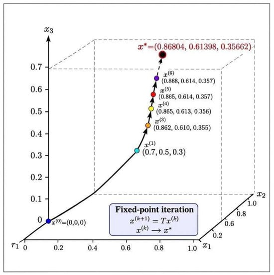
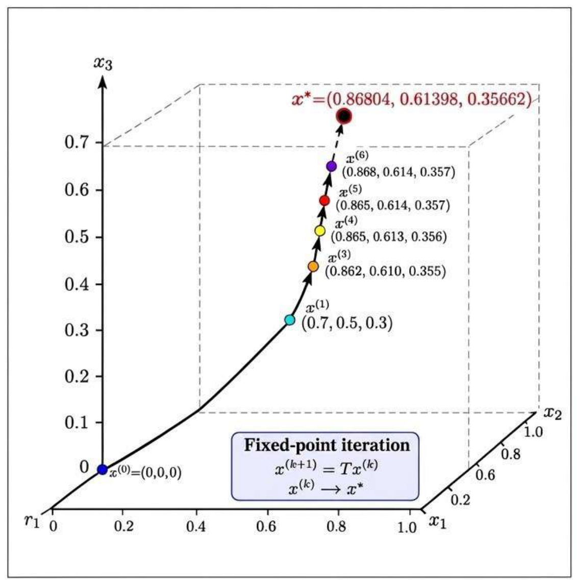
To demonstrate the applicability of the above result, we present a concrete numerical example that illustrates the geometric interpretation of Theorem 3 in ${\mathbb{R}}^3$. We consider a concrete $3\times 3$ matrix satisfying the required contractive condition and study the corresponding iterative process. Figure 1 depicts the resulting trajectory in three-dimensional space and illustrates its convergence toward the unique FP.

Figure 1. Numerical illustration in dimension 3 of the fixed-point approach to the linear system $Bx=r$.

Example 2.

Consider the linear system

$$Bu=r,$$

where

$$B=\left(\begin{array}{ccc}-0.85& 0.05& 0.02\\ 0.03& -0.88& 0.04\\ 0.01& 0.02& -0.90\end{array}\right),r=\left(\begin{array}{c}-0.7\\ -0.5\\ -0.3\end{array}\right).$$

Following the construction in Theorem 3, we set

$$A=I_3+B=\left(\begin{array}{ccc}0.15& 0.05& 0.02\\ 0.03& 0.12& 0.04\\ 0.01& 0.02& 0.10\end{array}\right).$$

Define $T\left(x\right)=Ax-r$. Explicitly,

$$T(x_1,x_2,x_3)=\left(\begin{array}{c}0.15x_1+0.05x_2+0.02x_3+0.7\\ 0.03x_1+0.12x_2+0.04x_3+0.5\\ 0.01x_1+0.02x_2+0.10x_3+0.3\end{array}\right).$$

Moreover,

$$T\left(x\right)=x⟺Ax-r=x⟺(I_3-A)x=-r⟺Bx=r.$$

We now verify the contraction condition of Theorem 3. Since $\lambda =\parallel I_3{+B\parallel }_{\infty }={\parallel A\parallel }_{\infty }$, we calculate the three row sums:

$${\displaystyle \sum _{j=1}^3}|a_{1j}|=0.22,{\displaystyle \sum _{j=1}^3}|a_{2j}|=0.19,{\displaystyle \sum _{j=1}^3}|a_{3j}|=0.13.$$

Therefore, $\lambda ={\parallel A\parallel }_{\infty }=max\{0.22,0.19,0.13\}=0.22$.

On the other hand, ${\displaystyle \frac{1}{1+\sqrt{6}}}\approx 0.2899.$ Consequently, $\lambda =0.22<0.2899={\displaystyle \frac{1}{1+\sqrt{6}}}$.

Thus, all the hypotheses of Theorem 3 are satisfied, and the linear system has a unique solution.

For completeness, the solution can be approximated by the fixed-point iteration

$$x^{(k+1)}=T\left(x^{\left(k\right)}\right),x^{\left(0\right)}=(0,0,0).$$

The first iterates are

$$\begin{array}{cc}\hfill x^{\left(1\right)}& =T\left(x^{\left(0\right)}\right)=(0.700000,0.500000,0.300000),\hfill \\ \hfill x^{\left(2\right)}& =T\left(x^{\left(1\right)}\right)=(0.836000,0.593000,0.347000),\hfill \\ \hfill x^{\left(3\right)}& =T\left(x^{\left(2\right)}\right)=(0.861990,0.610120,0.354920),\hfill \\ \hfill x^{\left(4\right)}& =T\left(x^{\left(3\right)}\right)=(0.866903,0.613271,0.356314),\hfill \\ \hfill x^{\left(5\right)}& =T\left(x^{\left(4\right)}\right)=(0.867825,0.613852,0.356566),\hfill \\ \hfill x^{\left(6\right)}& =T\left(x^{\left(5\right)}\right)=(0.867998,0.613960,0.356612).\hfill \end{array}$$

Hence, $x^{\left(k\right)}⟶x^{*}\mathit{as}k\to \infty$, where $x^{*}\approx (0.86804,0.61398,0.35662)$.

Indeed, direct substitution gives $B{x}^{*}\approx \left(\begin{array}{c}-0.7\\ -0.5\\ -0.3\end{array}\right)=r$, confirming that

$u^{*}=(0.86804,0.61398,0.35662)$ is the unique solution of the original linear system.

3.2. Application to a Second-Order Boundary Value Problem

Consider the boundary value problem

$$\left\{\begin{array}{cc}-w^{″}\left(t\right)=h(t,w\left(t\right)),\hfill & t\in [0,1],\hfill \\ w\left(0\right)=w\left(1\right)=0,\hfill & \end{array}\right.$$

(61)

where $h:[0,1]\times \mathbb{R}\to \mathbb{R}$ is continuous.

The Green function associated with the Dirichlet problem is

$$G(t,s)=\left\{\begin{array}{cc}t(1-s),\hfill & 0\le t\le s\le 1,\hfill \\ s(1-t),\hfill & 0\le s\le t\le 1.\hfill \end{array}\right.$$

A solution of (61) is equivalently an FP of the operator $F:C\left(\right[0,1],\mathbb{R})\to C\left(\right[0,1],\mathbb{R})$ defined by

$$\left(Fw\right)\left(t\right)={\int }_0^{1}G(t,s)h(s,w\left(s\right))ds.$$

Equip $C\left(\right[0,1],\mathbb{R})$ with

$$\underline{\mathcal{B}}(w,\rho )={\parallel w-\rho \parallel }_{\infty }^2{,\parallel w\parallel }_{\infty }=\underset{t\in [0,1]}{max}\left|w\left(t\right)\right|.$$

This is a complete b-metric space with $b=2$.

Theorem 4.

Assume that there exists a constant $L>0$ such that

$$\left|h\right(t,u)-h(t,v\left)\right|\le L|u-v|$$

for all $t\in [0,1]$ and all $u,v\in \mathbb{R}$, and suppose that

$$L<{\displaystyle \frac{8}{1+\sqrt{6}}}.$$

Then, the boundary value problem (61) has a unique solution $w^{*}\in C^2\left([0,1]\right)$.

Proof. 

The proof is obtained by an application of Corollary 2. More precisely, we shall verify that the operator associated with the boundary value problem satisfies all the hypotheses of this corollary. We first identify the underlying function space as a complete $(C-\underline{\mathcal{B}}m)$ space and then establish the Kannan-type contractive condition.

Let $X=C\left(\right[0,1],\mathbb{R})$ and define

$$\underline{\mathcal{B}}(w,\rho )={\parallel w-\rho \parallel }_{\infty }^2,w,\rho \in X,$$

where ${\parallel w-\rho \parallel }_{\infty }={max}_{t\in [0,1]}|w\left(t\right)-\rho \left(t\right)|$.

Since $C\left(\right[0,1],\mathbb{R})$, equipped with the supremum norm, is a Banach space, it remains only to verify that $\underline{\mathcal{B}}$ defines a complete b-metric.

Clearly,

$$\underline{\mathcal{B}}(w,\rho )\ge 0,$$

and

$$\underline{\mathcal{B}}(w,\rho )=0⟺{\parallel w-\rho \parallel }_{\infty }=0⟺w=\rho .$$

Moreover,

$$\underline{\mathcal{B}}(w,\rho )={\parallel w-\rho \parallel }_{\infty }^2={\parallel \rho -w\parallel }_{\infty }^2=\underline{\mathcal{B}}(\rho ,w).$$

For any $w,\rho ,z\in X$, the triangle inequality for the supremum norm gives

$${\parallel w-\rho \parallel }_{\infty }\le {\parallel w-z\parallel }_{\infty }+{\parallel z-\rho \parallel }_{\infty }.$$

Therefore,

$$\begin{array}{cc}\hfill \underline{\mathcal{B}}(w,\rho )& ={\parallel w-\rho \parallel }_{\infty }^2\hfill \\ & \le {\left({\parallel w-z\parallel }_{\infty }+{\parallel z-\rho \parallel }_{\infty }\right)}^2\hfill \\ & ={\parallel w-z\parallel }_{\infty }^2{+2\parallel w-z\parallel }_{\infty }{\parallel z-\rho \parallel }_{\infty }+{\parallel z-\rho \parallel }_{\infty }^2.\hfill \end{array}$$

Using $2ab\le a^2+b^2$, we obtain $\underline{\mathcal{B}}(w,\rho )\le {2\parallel w-z\parallel }_{\infty }^2+2{\parallel z-\rho \parallel }_{\infty }^2$, and hence

$$\underline{\mathcal{B}}(w,\rho )\le 2\left(\underline{\mathcal{B}}(w,z)+\underline{\mathcal{B}}(z,\rho )\right).$$

Thus, $\underline{\mathcal{B}}$ is a b-metric with coefficient $b=2$. Completeness follows directly from the completeness of $(C([0,1],\mathbb{R}),\parallel ·{\parallel }_{\infty })$.

Define the operator $F:X\to X$ by

$$\left(Fw\right)\left(t\right)={\int }_0^{1}G(t,s)h(s,w\left(s\right))ds,$$

where

$$G(t,s)=\left\{\begin{array}{cc}t(1-s),\hfill & 0\le t\le s\le 1,\hfill \\ s(1-t),\hfill & 0\le s\le t\le 1.\hfill \end{array}\right.$$

Since h is continuous and $w\in C\left(\right[0,1],\mathbb{R})$, the function $s⟼h(s,w(s\left)\right)$ is continuous on $[0,1]$. Since G is continuous on $[0,1]\times [0,1]$, it follows that

$$t⟼{\int }_0^{1}G(t,s)h(s,w\left(s\right))ds$$

is continuous. Consequently,

$$Fw\in C\left(\right[0,1],\mathbb{R}),$$

and hence F is indeed a self-map of X.

Let $w,\rho \in X$. For every $t\in [0,1]$, we have

$$\begin{array}{cc}\hfill \left|\right(Fw\left)\right(t)-(F\rho \left)\right(t\left)\right|& =\left|{\int }_0^{1}G(t,s)\left[h(s,w(s\left)\right)-h(s,\rho (s\left)\right)\right]ds\right|\hfill \\ & \le {\int }_0^{1}G(t,s)\left|h(s,w(s\left)\right)-h(s,\rho (s\left)\right)\right|ds.\hfill \end{array}$$

By the assumed Lipschitz condition,

$$\left|h\right(s,w\left(s\right))-h(s,\rho \left(s\right)\left)\right|\le L\left|w\right(s)-\rho (s\left)\right|,$$

so

$$\begin{array}{cc}\hfill \left|\right(Fw\left)\right(t)-(F\rho \left)\right(t\left)\right|& \le L{\int }_0^{1}G(t,s)|w\left(s\right)-\rho \left(s\right)|ds\hfill \\ & \le {L\parallel w-\rho \parallel }_{\infty }{\int }_0^{1}G(t,s)ds.\hfill \end{array}$$

For a fixed $t\in [0,1]$, using the definition of G,

$$\begin{array}{cc}\hfill {\int }_0^{1}G(t,s)ds& ={\int }_0^{t}s(1-t)ds+{\int }_t^{1}t(1-s)ds\hfill \\ & =(1-t){\int }_0^{t}sds+t{\int }_t^1(1-s)ds\hfill \\ & =(1-t){\displaystyle \frac{t^2}{2}}+t{\left[s-{\displaystyle \frac{s^2}{2}}\right]}_{s=t}^{s=1}\hfill \\ & ={\displaystyle \frac{t^2(1-t)}{2}}+t\left({\displaystyle \frac{1}{2}}-t+{\displaystyle \frac{t^2}{2}}\right)\hfill \\ & ={\displaystyle \frac{t^2-t^3}{2}}+{\displaystyle \frac{t}{2}}-t^2+{\displaystyle \frac{t^3}{2}}\hfill \\ & ={\displaystyle \frac{t(1-t)}{2}}.\hfill \end{array}$$

The function $t(1-t)$ attains its maximum at $t=1/2$, and therefore

$$\underset{t\in [0,1]}{sup}{\int }_0^{1}G(t,s)ds={\displaystyle \frac{1}{2}}\left({\displaystyle \frac{1}{2}}\right)\left(1-{\displaystyle \frac{1}{2}}\right)={\displaystyle \frac{1}{8}}.$$

Consequently,

$$|\left(Fw\right)\left(t\right)-\left(F\rho \right)\left(t\right)|\le {\displaystyle \frac{L}{8}}{\parallel w-\rho \parallel }_{\infty },$$

for every $t\in [0,1]$. Taking the supremum over t, we obtain

$${\parallel Fw-F\rho \parallel }_{\infty }\le {\displaystyle \frac{L}{8}}{\parallel w-\rho \parallel }_{\infty }.$$

Put $\mu ={\displaystyle \frac{L}{8}}$. Then, ${\parallel Fw-F\rho \parallel }_{\infty }\le \mu {\parallel w-\rho \parallel }_{\infty }$.

We now express the right-hand side in terms of the displacement quantities appearing in the Kannan contraction. Observe that

$$w-\rho =(w-Fw)+(Fw-F\rho )+(F\rho -\rho ).$$

Hence, by the triangle inequality,

$${\parallel w-\rho \parallel }_{\infty }\le {\parallel w-Fw\parallel }_{\infty }{+\parallel Fw-F\rho \parallel }_{\infty }+{\parallel F\rho -\rho \parallel }_{\infty }.$$

It follows that

$$\begin{array}{cc}\hfill {\parallel Fw-F\rho \parallel }_{\infty }& \le {\mu \parallel w-\rho \parallel }_{\infty }\hfill \\ & \le \mu \left({\parallel w-Fw\parallel }_{\infty }{+\parallel Fw-F\rho \parallel }_{\infty }+{\parallel F\rho -\rho \parallel }_{\infty }\right).\hfill \end{array}$$

Therefore,

$${(1-\mu )\parallel Fw-F\rho \parallel }_{\infty }\le \mu \left({\parallel w-Fw\parallel }_{\infty }+{\parallel \rho -F\rho \parallel }_{\infty }\right).$$

The hypothesis $L<{\displaystyle \frac{8}{1+\sqrt{6}}}$ implies $\mu ={\displaystyle \frac{L}{8}}<{\displaystyle \frac{1}{1+\sqrt{6}}}<1$.

Thus, $1-\mu >0$, and consequently,

$${\parallel Fw-F\rho \parallel }_{\infty }\le {\displaystyle \frac{\mu }{1-\mu }}\left({\parallel w-Fw\parallel }_{\infty }+{\parallel \rho -F\rho \parallel }_{\infty }\right).$$

Squaring both sides yields

$${\parallel Fw-F\rho \parallel }_{\infty }^2\le {\displaystyle \frac{{\mu }^2}{{(1-\mu )}^2}}{\left({\parallel w-Fw\parallel }_{\infty }+{\parallel \rho -F\rho \parallel }_{\infty }\right)}^2.$$

Using again ${(a+b)}^2\le 2(a^2+b^2)$, we obtain

$$\begin{array}{cc}\hfill {\parallel Fw-F\rho \parallel }_{\infty }^2& \le {\displaystyle \frac{2{\mu }^2}{{(1-\mu )}^2}}\left({\parallel w-Fw\parallel }_{\infty }^2+{\parallel \rho -F\rho \parallel }_{\infty }^2\right)\hfill \\ & ={\displaystyle \frac{2{\mu }^2}{{(1-\mu )}^2}}\left(\underline{\mathcal{B}}(w,Fw)+\underline{\mathcal{B}}(\rho ,F\rho )\right).\hfill \end{array}$$

Since

$$\underline{\mathcal{B}}(Fw,F\rho )={\parallel Fw-F\rho \parallel }_{\infty }^2,$$

we have

$$\underline{\mathcal{B}}(Fw,F\rho )\le {\Lambda }_1\left(\underline{\mathcal{B}}(w,Fw)+\underline{\mathcal{B}}(\rho ,F\rho )\right),$$

where ${\Lambda }_1={\displaystyle \frac{2{\mu }^2}{{(1-\mu )}^2}}$..

We verify explicitly the numerical condition required by Corollary 2. Since $\mu <{\displaystyle \frac{1}{1+\sqrt{6}}}$, we have $\sqrt{6}\mu <1-\mu$.

Both sides are positive, so squaring gives

$$6{\mu }^2<{(1-\mu )}^2.$$

Dividing by the positive number ${(1-\mu )}^2$, we obtain

$${\displaystyle \frac{6{\mu }^2}{{(1-\mu )}^2}}<1.$$

Since ${\Lambda }_1={\displaystyle \frac{2{\mu }^2}{{(1-\mu )}^2}}$, it follows that $3{\Lambda }_1={\displaystyle \frac{6{\mu }^2}{{(1-\mu )}^2}}<1$. Therefore, ${\Lambda }_1<{\displaystyle \frac{1}{3}}<{\displaystyle \frac{1}{2}}$.

Furthermore, because the coefficient of the b-metric is $b=2$,

$$b{\Lambda }_1+{\Lambda }_1=2{\Lambda }_1+{\Lambda }_1=3{\Lambda }_1<1.$$

Thus, F satisfies all the assumptions of Corollary 2. Hence, there exists a unique $w^{*}\in C([0,1],\mathbb{R})$ such that

$$F{w}^{*}=w^{*}.$$

Accordingly,

$$w^{*}\left(t\right)={\int }_0^{1}G(t,s)h(s,w^{*}\left(s\right))ds,t\in [0,1].$$

It remains to verify that this FP is a classical solution of the boundary value problem. Put

$$q\left(s\right)=h(s,w^{*}\left(s\right)).$$

Since h and $w^{*}$ are continuous, $q\in C\left(\right[0,1\left]\right)$. Using the explicit expression for G, the fixed-point equation becomes

$$w^{*}\left(t\right)=(1-t){\int }_0^{t}sq\left(s\right)ds+t{\int }_t^1(1-s)q\left(s\right)ds.$$

Differentiating and applying the Leibniz rule gives

$$\begin{array}{cc}\hfill w^{*\prime }\left(t\right)& =-{\int }_0^{t}sq\left(s\right)ds+(1-t)tq\left(t\right)\hfill \\ & +{\int }_t^1(1-s)q\left(s\right)ds-t(1-t)q\left(t\right).\hfill \end{array}$$

The two terms involving $t(1-t)q\left(t\right)$ cancel, and hence

$$w^{*\prime }\left(t\right)=-{\int }_0^{t}sq\left(s\right)ds+{\int }_t^1(1-s)q\left(s\right)ds.$$

Differentiating once more yields

$$\begin{array}{cc}\hfill w^{*″}\left(t\right)& =-tq\left(t\right)-(1-t)q\left(t\right)\hfill \\ & =-q\left(t\right)\hfill \\ & =-h(t,w^{*}\left(t\right)).\hfill \end{array}$$

Therefore,

$$-w^{*″}\left(t\right)=h(t,w^{*}\left(t\right)).$$

Moreover, evaluating the Green representation at $t=0$ gives

$$w^{*}\left(0\right)=0,$$

and evaluating it at $t=1$ gives

$$w^{*}\left(1\right)=0.$$

Since q is continuous, the above calculation also shows that $w^{*″}$ is continuous. Hence,

$$w^{*}\in C^2\left([0,1]\right).$$

Thus, $w^{*}$ is a classical solution of the boundary value problem. The uniqueness of the FP of F implies the uniqueness of the solution. Therefore, problem (61) has a unique solution in $C^2\left([0,1]\right)$. □

Example 3.

Consider the boundary value problem

$$\left\{\begin{array}{cc}-w^{″}\left(t\right)=w\left(t\right)+1,\hfill & t\in [0,1],\hfill \\ w\left(0\right)=w\left(1\right)=0.\hfill & \end{array}\right.$$

Consider the function $h(t,u)=u+1$, which is continuous on $[0,1]\times \mathbb{R}$, and for all $t\in [0,1]$ and $u,v\in \mathbb{R}$,

$$\left|h\right(t,u)-h(t,v\left)\right|=\left|\right(u+1)-(v+1\left)\right|=|u-v|.$$

Hence, the Lipschitz constant is $L=1$. Since ${\displaystyle \frac{8}{1+\sqrt{6}}}\approx 2.194,$ we have $L=1<{\displaystyle \frac{8}{1+\sqrt{6}}}.$

Therefore, all the hypotheses of the theorem are satisfied, and the boundary value problem has a unique solution.

Indeed, the associated fixed-point operator is

$$\left(Fw\right)\left(t\right)={\int }_0^{1}G(t,s)\left(w\left(s\right)+1\right)ds,$$

where

$$G(t,s)=\left\{\begin{array}{cc}t(1-s),\hfill & 0\le t\le s\le 1,\hfill \\ s(1-t),\hfill & 0\le s\le t\le 1.\hfill \end{array}\right.$$

For $w,\rho \in C\left(\right[0,1],\mathbb{R})$, we obtain

$$\begin{array}{cc}\hfill \left|\right(Fw\left)\right(t)-(F\rho \left)\right(t\left)\right|& =\left|{\int }_0^{1}G(t,s)\left(w\left(s\right)-\rho \left(s\right)\right)ds\right|\hfill \\ & \le {\int }_0^{1}G(t,s)|w\left(s\right)-\rho \left(s\right)|ds\hfill \\ & \le {\parallel w-\rho \parallel }_{\infty }{\int }_0^{1}G(t,s)ds.\hfill \end{array}$$

A direct calculation gives

$${\int }_0^{1}G(t,s)ds={\displaystyle \frac{t(1-t)}{2}}\le {\displaystyle \frac{1}{8}},t\in [0,1].$$

Consequently,

$${\parallel Fw-F\rho \parallel }_{\infty }\le {\displaystyle \frac{1}{8}}{\parallel w-\rho \parallel }_{\infty }.$$

Since $\underline{\mathcal{B}}(w,\rho )={\parallel w-\rho \parallel }_{\infty }^2$, it follows that

$$\begin{array}{cc}\hfill \underline{\mathcal{B}}(Fw,F\rho )& ={\parallel Fw-F\rho \parallel }_{\infty }^2\hfill \\ & \le {\displaystyle \frac{1}{64}}{\parallel w-\rho \parallel }_{\infty }^2\hfill \\ & ={\displaystyle \frac{1}{64}}\underline{\mathcal{B}}(w,\rho ).\hfill \end{array}$$

Thus, the induced contraction coefficient is $\Lambda ={\displaystyle \frac{1}{64}}.$ In particular, $\Lambda ={\displaystyle \frac{1}{64}}<{\displaystyle \frac{1}{1+\sqrt{6}}}$, so the fixed-point theorem applies directly.

Remark 3.

Under the global Lipschitz assumption on h, the classical Banach contraction principle yields the stronger numerical condition $L<8$. Indeed, the Green-function estimate gives

$${\parallel Fw-F\rho \parallel }_{\infty }\le {\displaystyle \frac{L}{8}}{\parallel w-\rho \parallel }_{\infty }.$$

However, the purpose of the present application is different: it illustrates how the Kannan-type fixed-point criterion established in Corollary 2 can be applied to the Green operator in the complete b-metric space $(C([0,1],\mathbb{R}),\underline{\mathcal{B}})$. The resulting Kannan coefficient is

$${\Lambda }_1=2{\left({\displaystyle \frac{L}{8-L}}\right)}^2,$$

and, since $b=2$, the condition $b{\Lambda }_1+{\Lambda }_1<1$ is satisfied whenever

$$L<{\displaystyle \frac{8}{1+\sqrt{6}}}.$$

Thus, the application demonstrates the applicability of the proposed Kannan/permutation framework rather than an improvement over the classical Banach contraction bound for this particular boundary value problem.

4. Conclusions and Further Perspectives

This paper set out an FP framework for permutation contractions in C-$\mathcal{B}m$ spaces. By arranging a weighted family of orbital distances through an arbitrary permutation, we obtained a generalized Banach-type FP theorem that secures both existence and uniqueness under a suitable contractive condition.

A second contribution lies in the per-term domination framework we introduced, where each orbital distance is bounded individually in terms of the underlying distance. Working within this framework, we were also able to recover Kannan-type contractions and a restricted version of the Hardy-Rogers condition once the weights and domination assumptions are chosen appropriately.

To test the applicability of these results, we considered two rather different problems. The first is a linear system of equations, where the FP formulation yields conditions guaranteeing the existence and uniqueness of the solution. The second is a second-order boundary value problem that is chosen precisely to show that the approach is not tied to finite-dimensional algebra and extends naturally to differential equations as well.

A number of questions remain open. Perhaps the most immediate is whether the per-term domination assumptions can be relaxed further—that is, whether individual orbital distances can still be controlled under weaker hypotheses without the permutation contraction collapsing back into an ordinary global Lipschitz condition. Beyond this, it would be worth exploring analogous results in other generalized metric structures and in multivalued, cyclic, or graph-based versions of permutation contractions. We hope these directions contribute to a broader theory of orbit-dependent contractions and to closer ties between generalized metric FP theory and its applications.

References

- Shehzad, U.; Batul, S.; Sagheer, D.E.S.; Ayoob, I.; Mlaiki, N. Fixed point results via fuzzy mappings in b-metric spaces and an application to differential equations. J. Inequalities Appl. 2025, 2025, 66. [Google Scholar] [CrossRef] [Scilit]
- Sonam, S.K.; Paul, S.K.; Bhardwaj, R. Exploring fixed point results in fuzzy bipolar metric spaces and application to differential equations. J. Comput. Appl. Math. 2026, 485, 117601. [Google Scholar] [CrossRef] [Scilit]
- Qawasmeh, T.; Malkawi, A.A. Fixed Point Theory in MR-Metric Spaces Fundamental Theorems and Applications to Integral Equations and Neutron Transport. Eur. J. Pure Appl. Math. 2025, 18, 6440. [Google Scholar] [CrossRef] [Scilit]
- Beg, I.; Ermis, T.; Gelisgen, Ö.; Abbas, M. Applications of Asymptotic Fixed Point Theorems in A-Metric Spaces to Integral Equations. J. Funct. Spaces 2025, 2025, 1727696. [Google Scholar] [CrossRef] [Scilit]
- Banach, S. Sur les opérations dans les ensembles abstraits et leur application aux équations intégrales. Fund. Math. 1922, 3, 133–181. [Google Scholar] [CrossRef] [Scilit]
- Kannan, R. Some results on fixed points. Bull. Cal. Math. Soc. 1968, 60, 71–76. [Google Scholar]
- Reich, S. Kannan’s fixed point theorem. Boll. Un. Mat. Ital. 1971, 4, 1–11. [Google Scholar]
- Saikia, J.; Debnath, P. Fixed points and attractors of iterated function systems via generalized enriched Kannan-type cyclic contractions. Optimization 2026, 1–21. [Google Scholar] [CrossRef] [Scilit]
- Chatterjea, S.K. Fixed-point theorems. Comptes Rendus de L’Académie Bulgare des Sci. 1972, 25, 727–730. [Google Scholar]
- Branciari, A. A fixed point theorem of Banach-Caccioppoli type on a class of generalized metric spaces. Publ. Math. 2000, 57, 31–37. [Google Scholar] [CrossRef] [Scilit]
- Mlaiki, N.; Hajji, M.; Abdeljawad, T. A New Extension of the Rectangular b-Metric Spaces. Adv. Math. Phys. 2020, 2020, 8319584. [Google Scholar] [CrossRef] [Scilit]
- Matthews, S.G. Partial metric topology. Ann. N. Y. Acad. Sci. 1994, 728, 183–197. [Google Scholar] [CrossRef] [Scilit]
- Huang, M.; Jia, X.; Li, Q. Topologies and fixpoints on weak partial metric spaces. Topol. Its Appl. 2026, 377, 109601. [Google Scholar] [CrossRef] [Scilit]
- Czerwik, S. Contraction mappings in b-metric spaces. Acta Math. Inform. Univ. Ostrav. 1993, 1, 5–11. [Google Scholar]
- Devi, M.; Chauhan (Gonder), S.S.; Shukla, R. Computational Analysis of Common Fixed Points in b-Metric Spaces with Applications to Well-Posedness and Projectile Motion. Int. J. Differ. Equ. 2026, 2026, 5593734. [Google Scholar] [CrossRef] [Scilit]
- Alsulami, S.M.; Alarfaj, T.A. Fixed-Point Results for Ćirić Contraction Mappings in Strong b-Metric Spaces. Axioms 2026, 15, 463. [Google Scholar] [CrossRef] [Scilit]
- Ayoob, I.; Mlaiki, N. A generalized fixed point theorem via permutation contractions with an application to integral equations. Bound. Value Probl. 2026, 2026, 126. [Google Scholar] [CrossRef] [Scilit]
Disclaimer/Publisher’s Note: The statements, opinions and data contained in all publications are solely those of the individual author(s) and contributor(s) and not of MDPI and/or the editor(s). MDPI and/or the editor(s) disclaim responsibility for any injury to people or property resulting from any ideas, methods, instructions or products referred to in the content. |
© 2026 by the author. Licensee MDPI, Basel, Switzerland. This article is an open access article distributed under the terms and conditions of the Creative Commons Attribution (CC BY) license.