Equivariant Cohomology for Slice Groupoids and Its Local Linear Models

Abstract

Let G be a compact Lie group acting smoothly on a manifold M. The local structure of such actions is described by the slice theorem, which reduces the study of G-spaces to smaller isotropy group actions. In this paper, we investigate the equivariant cohomology of these local models from the viewpoint of Weil and Cartan complexes. We construct explicit reduction morphisms between the equivariant cohomology complexes associated with a slice neighborhood $G{ \times }_{G_x}{S}_x$ and the slice $S_x$ with the isotropy group $G_x$. We prove that these morphisms induce isomorphisms in equivariant cohomology. Based on this local description, we introduce slice groupoids, a class of groupoids locally modeled on Lie group actions, and define their equivariant cohomology using sheaf-theoretic methods. Finally, we show that for slice groupoids arising from action groupoids, the resulting cohomology agrees with the classical equivariant cohomology of the underlying group action.

1. Equivariant Cohomology

1.1. Introduction

The topology and cohomology of a G-space M and of the quotient space $M/G$ arise in many branches of geometry. Let M be a manifold. In general, if G does not act freely on M, the quotient space may be singular even though M is smooth. From the viewpoint of equivariant homotopy theory, one is naturally led to the equivariant cohomology of M. Throughout this paper, group actions on manifolds are taken to be left actions. Let $E_G$ be a contractible space equipped with a free right G-action (see [1] for the existence of $E_G$). For a left G-space M, define the Borel construction by

$$E_G{ \times }_{G}M=(E_G\times M)/G,$$

where G acts freely from the right on $E_G\times M$ by

$$(p,x)·g=(pg,g^{-1}·x).$$

Equivalently, the quotient relation is

$$[p,x]=[pg,g^{-1}·x].$$

The equivariant cohomology of M is defined by

$$H_G^{\ast }(M;\mathbb{R})=H^{\ast }(E_G{ \times }_{G}M;\mathbb{R}).$$

Throughout this paper, all cohomology groups are taken with coefficients in $\mathbb{R}$, unless otherwise stated. Accordingly, $H_G^{\ast }\left(M\right)$ denotes $H^{\ast }(E_G{ \times }_{G}M;\mathbb{R})$, and all de Rham, Weil, and Cartan complexes are considered over $\mathbb{R}$.

Since the right G-action on $E_G$ is free, the induced right action

$$(p,x)·g=(pg,g^{-1}·x)$$

on $E_G\times M$ is free. In particular, if G acts freely on M, then $M/G$ is a manifold, and the equivariant cohomology is naturally isomorphic to the ordinary cohomology of $M/G$ [2]. One may also consider a de Rham realization of the equivariant cohomology. Formally, this is related to differential forms on the Borel construction $E_G{ \times }_{G}M$. Since $E_G$ is generally infinite dimensional when G is nontrivial, one usually uses finite-dimensional approximations, or an equivalent algebraic model such as the Weil or Cartan model.

A convenient way to compute the equivariant cohomology of M is to replace the complex ${\Omega }^{\ast }\left(E_G{ \times }_{G}M\right)$ by an algebraic model. The Weil model is the complex of basic elements ${[\Omega \left(M\right)\otimes \Lambda \left({\mathfrak{g}}^{\ast }\right)\otimes S\left({\mathfrak{g}}^{\ast }\right)]}_{\mathrm{bas}}$, while the Cartan model is the complex of invariant elements ${[\Omega \left(M\right)\otimes S\left({\mathfrak{g}}^{\ast }\right)]}^G$, equipped with an appropriate differential. When G is compact, the cohomology groups of both complexes are isomorphic to equivariant cohomology. The explicit constructions of the Weil and Cartan models are given as follows; see [1].

Let G be an m-dimensional Lie group, let $\{{\xi }_1,\dots ,{\xi }_m\}$ be a basis of its Lie algebra $\mathfrak{g}$, and let $\{x^1,\dots ,x^m\}$ be the dual basis of ${\mathfrak{g}}^{\ast }$. We use the Einstein summation convention $[{\xi }_i,{\xi }_j]=c_{ij}^k{\xi }_k$ for the Lie bracket. If $H\subset G$ is a closed Lie subgroup, choose $\{{\xi }_1,\dots ,{\xi }_t\}$ to be a basis of its Lie algebra $\mathfrak{h}$. Then

$$c_{ij}^k=0,$$

when $i,j\le t$ and $k>t$.

Let

$$\begin{array}{cc}\hfill {\theta }^i=& x^i\otimes 1\in {\Lambda }^1\left({\mathfrak{g}}^{\ast }\right)\otimes S^0\left({\mathfrak{g}}^{\ast }\right)\hfill \\ \hfill z^i=& 1\otimes x^i\in {\Lambda }^0\left({\mathfrak{g}}^{\ast }\right)\otimes S^1\left({\mathfrak{g}}^{\ast }\right),\hfill \end{array}$$

then the Weil algebra $W\left({\mathfrak{g}}^{\ast }\right)=\Lambda \left({\mathfrak{g}}^{\ast }\right)\otimes S\left({\mathfrak{g}}^{\ast }\right)$ is generated by ${\theta }^1,\dots ,{\theta }^m,z^1,\dots ,z^m$, with

$$\begin{array}{c}\hfill {\theta }^i{\theta }^j=(x^i\wedge x^j)\otimes 1,z^i{z}^j=1\otimes x^i{x}^j\end{array}$$

and

$${\theta }^{i_1}\cdots {\theta }^{i_p}{z}^{j_1}\cdots z^{j_q}=(x^{i_1}\wedge \cdots \wedge x^{i_p})\otimes (x^{j_1}\cdots x^{j_q}).$$

The degree of an element ${\theta }^{i_1}\cdots {\theta }^{i_p}{z}^{j_1}\cdots z^{j_q}\in W\left({\mathfrak{g}}^{\ast }\right)$ is defined to be $p+2q$. The collection of all degree d elements in $W\left({\mathfrak{g}}^{\ast }\right)$ is denoted by $W^d\left({\mathfrak{g}}^{\ast }\right)$.

There are three operators on the Weil algebra. The Lie derivative on the Weil algebra is defined by

$${\mathcal{L}}_{{\xi }_a}{\theta }^b=-c_{ak}^b{\theta }^k$$

and

$${\mathcal{L}}_{{\xi }_a}{z}^b=-c_{ak}^b{z}^k.$$

The differential $\delta$ on the Weil algebra is defined by

$$\delta {\theta }^a=z^a,\delta z^a=0.$$

The interior operator $\iota$ on the Weil algebra is defined by

$${\iota }_{{\xi }_a}{\theta }^b={\delta }_a^b,{\iota }_{{\xi }_a}{z}^b=-c_{ak}^b{\theta }^k,$$

and these operators are extended as derivations to all of W.

From now on we use ${\mathcal{L}}_a$ and ${\iota }_a$ to replace ${\mathcal{L}}_{{\xi }_a}$ and ${\iota }_{{\xi }_a}$ to simplify the notation once the basis ${\left\{{\xi }_a\right\}}_{a=1}^m$ has been fixed.

Let ${[\Omega \left(M\right)\otimes W\left({\mathfrak{g}}^{\ast }\right)]}_{\mathrm{bas},G}\subset \Omega \left(M\right)\otimes W\left({\mathfrak{g}}^{\ast }\right)$ denote the subspace consisting of elements $\sigma \in \Omega \left(M\right)\otimes W\left({\mathfrak{g}}^{\ast }\right)$ such that ${\mathcal{L}}_a\sigma =0$ and ${\iota }_a\sigma =0$. Note that ${\mathcal{L}}_a$ is computed by the Leibniz rule and

$${\iota }_a={\iota }_a\otimes 1+1\otimes {(-1)}^p{\iota }_a$$

when applied to an element ${\alpha }^{p,q}\in {\Omega }^p\left(M\right)\otimes W^q\left({\mathfrak{g}}^{\ast }\right)$ for $a=1,\cdots ,m$. Then the Weil model is defined as the graded algebra

$$\mathrm{Weil}(M,G)=\underset{d\ge 0}{⨁}{\mathrm{Weil}}^d(M,G)$$

where

$${\mathrm{Weil}}^d(M,G)=\underset{p+q=d}{⨁}{[{\Omega }^p\left(M\right)\otimes W^q\left({\mathfrak{g}}^{\ast }\right)]}_{\mathrm{bas},G}$$

with the graded differential operator

$$D=d\otimes 1+{(-1)}^{p}1\otimes \delta .$$

The complex $\mathrm{Weil}(M,G)$ with differential D is called the Weil model; in the rest of the paper we write $\mathrm{Weil}(M,G)$ for the differential graded algebra $\left(\mathrm{Weil}\right(M,G),D)$. We call an element $\tau \in \Omega \left(M\right)\otimes W\left({\mathfrak{g}}^{\ast }\right)$ G-invariant if ${\mathcal{L}}_a\tau =0$ for every a, and G-horizontal if ${\iota }_a\tau =0$ for every a. If $\tau$ is both horizontal and invariant, then it is called a basic element. Thus, the Weil model $\mathrm{Weil}(M,G)$ is the graded algebra of basic elements in $\Omega \left(M\right)\otimes W\left({\mathfrak{g}}^{\ast }\right)$ equipped with the differential D. The operators D, ${\iota }_a$, and ${\mathcal{L}}_a$ satisfy the Cartan homotopy formula

$${\mathcal{L}}_a=[D,{\iota }_a]=D{\iota }_a+{\iota }_{a}D.$$

To construct the Cartan model, let

$$u^a=z^a+{\displaystyle \frac{1}{2}}{c}_{jk}^a{\theta }^j{\theta }^k$$

(1)

define a change of variables. Then, we have

$$\begin{array}{cc}\hfill d{u}^a& =-c_{ij}^a{\theta }^i{u}^j\hfill \\ \hfill {\mathcal{L}}_a{u}^b& =-c_{ak}^b{u}^k\hfill \\ \hfill {\iota }_a{u}^b& =0.\hfill \end{array}$$

Note that the new generators $u^a$ are horizontal. If $u^b$ is invariant (i.e., ${\mathcal{L}}_a{u}^b=0$ for any a), then $u^b=z^b$.

After this change of variables, $W\left({\mathfrak{g}}^{\ast }\right)$ is generated by $\{{\theta }^1,\dots ,{\theta }^m,u^1,\dots ,u^m\}$. Since ${\iota }_a{\theta }^b={\delta }_a^b$, the horizontal subalgebra is $W{\left({\mathfrak{g}}^{\ast }\right)}_{\mathrm{hor}}=1\otimes S\left({\mathfrak{g}}^{\ast }\right)$, and the basic subalgebra is $W{\left({\mathfrak{g}}^{\ast }\right)}_{\mathrm{bas}}=1\otimes S{\left({\mathfrak{g}}^{\ast }\right)}^G\cong S{\left({\mathfrak{g}}^{\ast }\right)}^G$, where $S{\left({\mathfrak{g}}^{\ast }\right)}^G$ denotes the G-invariant subalgebra. Let $\gamma ={\sum }_a{\iota }_a\otimes {\theta }^a$ be an endomorphism of $\Omega \left(M\right)\otimes W\left({\mathfrak{g}}^{\ast }\right)$ such that

$$\gamma (\omega \otimes \alpha )=\sum _a{\iota }_a\omega \otimes {\theta }^a\alpha ,$$

Define

$$\Phi =e^{\gamma }=1+\gamma +{\displaystyle \frac{1}{2}}{\gamma }^2+{\displaystyle \frac{1}{3!}}{\gamma }^3+\cdots ,$$

Then $\Phi$ is an automorphism of $\Omega \left(M\right)\otimes W\left({\mathfrak{g}}^{\ast }\right)$ known as the Mathai–Quillen isomorphism [3]. In particular, $\Phi$ carries ${[\Omega \left(M\right)\otimes W\left({\mathfrak{g}}^{\ast }\right)]}_{\mathrm{hor}}$ into $\Omega \left(M\right)\otimes {\left[W\left({\mathfrak{g}}^{\ast }\right)\right]}_{\mathrm{hor}}$, hence we have the restriction

$$\Phi :{[\Omega \left(M\right)\otimes W\left({\mathfrak{g}}^{\ast }\right)]}_{\mathrm{bas}}\to {[\Omega \left(M\right)\otimes S\left({\mathfrak{g}}^{\ast }\right)]}^G.$$

Moreover, $\Phi$ defines a differential $D_C$ on ${[\Omega \left(M\right)\otimes S\left({\mathfrak{g}}^{\ast }\right)]}^G$ by

$$D_C=\Phi D{\Phi }^{-1}=d\otimes 1-\sum _a{\iota }_a\otimes u^a.$$

The differential graded algebra ${[\Omega \left(M\right)\otimes S\left({\mathfrak{g}}^{\ast }\right)]}^G$ with differential $D_C$ is called the Cartan model and is denoted by $\mathrm{Car}(M,G)$.

The Weil and Cartan models can be used to compute equivariant de Rham cohomology. This is a classical result; see [1]. Explicitly,

Theorem 1. 

When G is compact, the cohomology of the Weil model and the cohomology of the Cartan model are isomorphic to the equivariant de Rham cohomology.

The equivariant de Rham isomorphism

$${\mathcal{DR}}_{G,M}:H^{\ast }\left(\mathrm{Car}(M,G)\right)\to H^{\ast }\left(E_G{ \times }_{G}M\right)$$

is the composition of the Mathai–Quillen identification between the Weil and Cartan models and the Weil realization induced by the universal connection on $E_G$. See [1] (Chapters 2–4).

1.2. Local Models

Now, we derive local properties of the equivariant cohomology. Assume that G acts properly on M, and let

$$\pi :M\to M/G$$

be the quotient map. Let $y\in M/G$, and let $U_y$ be a sufficiently small neighborhood of y. By the slice theorem, for such a neighborhood $U_y\subset M/G$, the inverse image ${\pi }^{-1}\left(U_y\right)$ is G-equivariantly diffeomorphic to $G{ \times }_{G_x}{S}_x$, where $x\in {\pi }^{-1}\left(y\right)$, $S_x$ is a $G_x$-invariant slice, and $G_x$ acts freely from the right on $G\times S_x$ by

$$(g,z)·h=(gh,h^{-1}·z),h\in G_x.$$

Thus the quotient relation is

$$[g,z]=[gh,h^{-1}·z].$$

The left G-action on $G{ \times }_{G_x}{S}_x$ is given by

$$k·[g,z]=[kg,z].$$

By definition,

$$H_G^{\ast }(G{ \times }_{G_x}{S}_x;\mathbb{R})=H^{\ast }\left(E_G{ \times }_G\left(G{\times }_{G_x}{S}_x\right);\mathbb{R}\right).$$

Since the right G-action on $E_G$ restricts to a free right $G_x$-action, the same space $E_G$ may also be used as a model for $E_{G_x}$. Define

$$\begin{array}{cc}\hfill f:E_G{ \times }_G\left(G{\times }_{G_x}{S}_x\right)& ⟶E_G{ \times }_{G_x}{S}_x,\hfill \\ \hfill [p,[g,z\left]\right]& ⟼[pg,z].\hfill \end{array}$$

We first check that f is well defined with respect to the G-quotient. For $k\in G$,

$$[p,[g,z]]=[pk,k^{-1}·[g,z]]=[pk,[k^{-1}g,z]],$$

and hence

$$f\left([pk,[k^{-1}g,z]]\right)=[pk{k}^{-1}g,z]=[pg,z].$$

It is also well defined with respect to the $G_x$-quotient. Indeed, if

$$[g,z]=[gh,h^{-1}z],h\in G_x,$$

then

$$f\left([p,[gh,h^{-1}z]]\right)=[pgh,h^{-1}z]=[pg,z]$$

in $E_G{ \times }_{G_x}{S}_x$. Define

$$\begin{array}{cc}\hfill f^{-1}:E_G{ \times }_{G_x}{S}_x& ⟶E_G{ \times }_G\left(G{\times }_{G_x}{S}_x\right),\hfill \\ \hfill [p,z]& ⟼[p,[e,z\left]\right].\hfill \end{array}$$

This map is well defined. For $h\in G_x$,

$$\begin{array}{cc}\hfill f^{-1}\left([ph,h^{-1}z]\right)& =[ph,[e,h^{-1}z]]\hfill \\ & =[ph,[h^{-1},z]]\hfill \\ & =[p,[e,z\left]\right].\hfill \end{array}$$

Moreover,

$$f\circ f^{-1}={\mathrm{id}}_{E_G{\times }_{G_x}{S}_x}$$

and

$$f^{-1}\circ f={\mathrm{id}}_{E_G{ \times }_G\left(G{ \times }_{G_x}{S}_x\right)}.$$

Therefore f is a homeomorphism. Consequently,

$$H_G^{\ast }(G{ \times }_{G_x}{S}_x;\mathbb{R})\cong H_{G_x}^{\ast }(S_x;\mathbb{R}).$$

Let $x_1,x_2\in {\pi }^{-1}\left(y\right)$ with $g·x_1=x_2$, and let $G_{x_i}$ denote the isotropy group of $x_i$. Then, for $h_1\in G_{x_1}$,

$$g{h}_1{g}^{-1}·x_2=g{h}_1{g}^{-1}g·x_1=g{h}_1·x_1=g·x_1=x_2,$$

hence, the isotropy group of $x_2$ is $g{G}_{x_1}{g}^{-1}$. Note that the slices $S_{x_1}$ and $S_{x_2}$ are homeomorphic and the quotient spaces $S_{x_i}/G_{x_i}$ and ${\pi }^{-1}\left(U_y\right)/G$ are homeomorphic.

The preceding homeomorphism suggests that the local equivariant cohomology of a proper G-action is determined by the isotropy action on a slice. A chain-level version of this statement will be proved in Theorem 3. In particular, for a sufficiently small $G_x$-invariant slice $S_x$, we will obtain

$$H_G^{\ast }({\pi }^{-1}\left(U_y\right);\mathbb{R})\cong H_{G_x}^{\ast }(S_x;\mathbb{R}).$$

Let M be a manifold with an action of a compact Lie group G. In addition to equivariant cohomology, one may also consider other cohomology theories such as $H^{\ast }(M/G)$, $H^{\ast }(\Omega {\left(M\right)}_{\mathrm{bas},G})$. The relations between these cohomology theories have been studied (see [4] for more details).

In fact, when $M\cong {\mathbb{R}}^n$, the cohomology of the complex ${\mathrm{Weil}}^{\ast ,0}({\mathbb{R}}^n,G)$

$$0\to {\Omega }^0{\left({\mathbb{R}}^n\right)}_{\mathrm{bas},G}\to {\Omega }^1{\left({\mathbb{R}}^n\right)}_{\mathrm{bas},G}\to \cdots$$

vanishes in degree $i>0$. This follows from the de Rham-type theorem for orbit spaces [5] together with the Conner conjecture [6]. The Conner conjecture asserts that the orbit space of any action of a compact Lie group on ${\mathbb{R}}^n$ is contractible. The Conner conjecture was proved by R. Oliver [7]. Related results can be found in Conner [6], Conner and Floyd [8,9], and Floyd [10].

1.3. Free Lie Group Actions

Let G be a compact Lie group acting smoothly and freely on a smooth manifold M. Since a compact group action is proper, the orbit space $M/G$ is a smooth manifold and the quotient map

$$\pi :M⟶M/G$$

is a principal G-bundle.

Let $\mathfrak{g}$ be the Lie algebra of G. Since G is compact, there exists a G-invariant Riemannian metric on M. The orthogonal complement of the tangent spaces to the G-orbits defines a G-invariant horizontal distribution and, hence, a principal connection $A\in {\Omega }^1(M;\mathfrak{g}).$ The connection form satisfies

$$A\left(X_{\xi }\right)=\xi ,{\phi }_g^{\ast }A={\mathrm{Ad}}_{g^{-1}}A$$

for every $\xi \in \mathfrak{g}$ and $g\in G$, where $X_{\xi }$ is the fundamental vector field generated by $\xi$ and ${\phi }_g:M\to M$ is the diffeomorphism defined by the G-action. Let

$$F_A=dA+{\displaystyle \frac{1}{2}}[A,A]\in {\Omega }^2(M;\mathfrak{g})$$

and ${\xi }_1,\dots ,{\xi }_m$ be a basis of $\mathfrak{g}$, with dual basis $x^1,\dots ,x^m$, write

$$A=\sum _a{A}^a{\xi }_a,F_A=\sum _a{F}_A^a{\xi }_a.$$

Recall that the Weil algebra $W\left({\mathfrak{g}}^{\ast }\right)$ is generated by elements ${\theta }^a$ of degree 1 and $u^a$ of degree 2. The connection A determines the Weil homomorphism

$$w_A:W\left({\mathfrak{g}}^{\ast }\right)⟶\Omega \left(M\right)$$

defined on generators by

$$w_A\left({\theta }^a\right)=A^a,w_A\left(u^a\right)=F_A^a.$$

The structure equations for A and the Bianchi identity imply that $w_A$ commutes with the differentials and is compatible with the contraction and Lie derivative operators.

Define

$${\mathcal{W}}_A:\Omega \left(M\right)\otimes W\left({\mathfrak{g}}^{\ast }\right)⟶\Omega \left(M\right)$$

by

$${\mathcal{W}}_A(\omega \otimes \sigma )=\omega \wedge w_A\left(\sigma \right).$$

Its restriction to the basic subcomplex gives a chain map

$${\mathcal{W}}_A:\mathrm{Weil}(M,G)⟶\Omega {\left(M\right)}_{\mathrm{bas}}.$$

Since the action is free and proper, pullback by the quotient map induces an isomorphism of differential graded algebras

$${\pi }^{\ast }:\Omega (M/G)\stackrel{\cong }{\to }\Omega {\left(M\right)}_{\mathrm{bas}}.$$

Consequently, the composition

$${\left({\pi }^{\ast }\right)}^{-1}\circ {\mathcal{W}}_A:\mathrm{Weil}(M,G)⟶\Omega (M/G)$$

is a quasi-isomorphism. Therefore,

$$H^{\ast }\left(\mathrm{Weil}(M,G)\right)\cong H_{\mathrm{dR}}^{\ast }(M/G)\cong H_G^{\ast }(M;\mathbb{R}).$$

The induced isomorphism in cohomology is independent of the chosen connection.

Now, let $U_y\subset M/G$ be a sufficiently small open neighborhood and let $S\subset {\pi }^{-1}\left(U_y\right)$ be a slice. Since the action is free, the isotropy group of every point is trivial and

$${\pi }^{-1}\left(U_y\right)\cong S\times G.$$

Moreover, the restriction

$${\pi |}_S:S⟶U_y$$

is a diffeomorphism. If

$$i_S:S\hookrightarrow {\pi }^{-1}\left(U_y\right)$$

denotes the inclusion, define

$${\mathcal{W}}_S=i_S^{\ast }\circ {\mathcal{W}}_A:\mathrm{Weil}({\pi }^{-1}\left(U_y\right),G)⟶\Omega \left(S\right).$$

Since

$$\Omega \left(S\right)=\mathrm{Weil}(S,e),$$

the map ${\mathcal{W}}_S$ may equivalently be regarded as a chain map

$${\mathcal{W}}_S:\mathrm{Weil}({\pi }^{-1}\left(U_y\right),G)⟶\mathrm{Weil}(S,e).$$

It is a quasi-isomorphism and hence induces an isomorphism

$$H^{\ast }\left(\mathrm{Weil}({\pi }^{-1}\left(U_y\right),G)\right)\cong H^{\ast }\left(\mathrm{Weil}(S,e)\right)=H_{\mathrm{dR}}^{\ast }\left(S\right).$$

The analogous statement for the Cartan model follows from the Mathai–Quillen isomorphism [3].

When the G-action is not free, the quotient map is no longer a principal G-bundle, and a global principal connection form satisfying $A\left(X_{\xi }\right)=\xi$ cannot exist, since some fundamental vector fields may vanish. In the next section, we construct a local reduction map adapted to the slice model $G{\times }_{G_x}{S}_x$.

2. Reduction over an Induced $\mathit{G}$-Manifold

Let G be a compact Lie group, let $H\subset G$ be a closed subgroup, and let S be a smooth H-manifold. We consider the induced G-manifold

$$M=G{ \times }_{H}S,$$

where H acts freely on $G\times S$ from the right by

$$(g,s)·h=(gh,h^{-1}·s).$$

(2)

The equivalence class of $(g,s)$ is denoted by $[g,s]$. The group G acts on M from the left by

$$k·[g,s]=[kg,s].$$

Let $𝚥:H\hookrightarrow G$ denote the inclusion homomorphism, and let

$$i:S⟶G{ \times }_{H}S,i\left(s\right)=[e,s],$$

be the natural inclusion. We regard $G{ \times }_{H}S$ as an H-manifold by restricting the G-action along 𝚥. Then i is H-equivariant. Indeed, for every $h\in H$,

$$i(h·s)=[e,h·s]=[h,s]=h·[e,s]=h·i\left(s\right).$$

This equivariant pair

$$(𝚥,i):(H,S)⟶(G,G{ \times }_{H}S)$$

will be used to define the reduction morphisms in both the Weil and Cartan models.

2.1. Reduction Map of the Weil and Cartan Models

We use the standard notation

$$W\left({\mathfrak{g}}^{\ast }\right)=\Lambda \left({\mathfrak{g}}^{\ast }\right)\otimes S\left({\mathfrak{g}}^{\ast }\right)$$

for the Weil algebra of ${\mathfrak{g}}^{\ast }$. The Lie algebra homomorphism

$$𝚥:\mathfrak{h}\hookrightarrow \mathfrak{g}$$

induces a morphism of differential graded algebras

$$W\left(𝚥\right):W\left({\mathfrak{g}}^{\ast }\right)⟶W\left({\mathfrak{h}}^{\ast }\right).$$

On generators, $W\left(𝚥\right)$ is induced by the restriction map

$${𝚥}^{\ast }:{\mathfrak{g}}^{\ast }⟶{\mathfrak{h}}^{\ast }.$$

More explicitly, if $\lambda \in {\mathfrak{g}}^{\ast }$, then

$$W\left(𝚥\right)\left({\theta }_{\lambda }\right)={\theta }_{{𝚥}^{\ast }\lambda },W\left(𝚥\right)\left(u_{\lambda }\right)=u_{{𝚥}^{\ast }\lambda }.$$

Define

$${\widetilde{\mathrm{Red}}}_W=i^{\ast }\otimes W\left(𝚥\right):\Omega \left(G{ \times }_{H}S\right)\otimes W\left({\mathfrak{g}}^{\ast }\right)⟶\Omega \left(S\right)\otimes W\left({\mathfrak{h}}^{\ast }\right).$$

Thus,

$${\widetilde{\mathrm{Red}}}_W(\omega \otimes \sigma )=i^{\ast }\omega \otimes W\left(𝚥\right)\left(\sigma \right).$$

Lemma 1. 

For every $\eta \in \mathfrak{h}$, the map ${\widetilde{\mathrm{Red}}}_W$ satisfies

$$\begin{array}{cc}\hfill {\iota }_{\eta }^H\circ {\widetilde{\mathrm{Red}}}_W& ={\widetilde{\mathrm{Red}}}_W\circ {\iota }_{𝚥\left(\eta \right)}^G,\hfill \end{array}$$

(3)

$$\begin{array}{cc}\hfill {\mathcal{L}}_{\eta }^H\circ {\widetilde{\mathrm{Red}}}_W& ={\widetilde{\mathrm{Red}}}_W\circ {\mathcal{L}}_{𝚥\left(\eta \right)}^G,\hfill \end{array}$$

(4)

$$\begin{array}{cc}\hfill D_H\circ {\widetilde{\mathrm{Red}}}_W& ={\widetilde{\mathrm{Red}}}_W\circ D_G.\hfill \end{array}$$

(5)

Proof. 

Since i is H-equivariant with respect to the inclusion $𝚥:H\hookrightarrow G$, the fundamental vector fields are i-related:

$$T_{s}i\left(X_{\eta }^S\left(s\right)\right)=X_{𝚥\left(\eta \right)}^{G{ \times }_{H}S}\left(i\left(s\right)\right).$$

(6)

Therefore,

$$\begin{array}{cc}\hfill i^{\ast }\circ {\iota }_{X_{𝚥\left(\eta \right)}}& ={\iota }_{X_{\eta }}\circ i^{\ast },\hfill \\ \hfill i^{\ast }\circ {\mathcal{L}}_{X_{𝚥\left(\eta \right)}}& ={\mathcal{L}}_{X_{\eta }}\circ i^{\ast }.\hfill \end{array}$$

On the Weil algebra, functoriality gives

$$\begin{array}{cc}\hfill {\iota }_{\eta }\circ W\left(𝚥\right)& =W\left(𝚥\right)\circ {\iota }_{𝚥\left(\eta \right)},\hfill \\ \hfill {\mathcal{L}}_{\eta }\circ W\left(𝚥\right)& =W\left(𝚥\right)\circ {\mathcal{L}}_{𝚥\left(\eta \right)},\hfill \\ \hfill d_{W\left(\mathfrak{h}\right)}\circ W\left(𝚥\right)& =W\left(𝚥\right)\circ d_{W\left({\mathfrak{g}}^{\ast }\right)}.\hfill \end{array}$$

Combining these identities with the definition of the total contraction, Lie derivative, and differential proves (3)–(5). □

Proposition 1. 

The map ${\widetilde{\mathrm{Red}}}_W$ sends G-basic elements to H-basic elements. Hence, it restricts to a morphism of differential graded algebras

$${\mathrm{Red}}_W:\mathrm{Weil}(G{ \times }_{H}S,G)⟶\mathrm{Weil}(S,H).$$

Proof. 

Let

$$\alpha \in \mathrm{Weil}(G{ \times }_{H}S,G).$$

For every $\eta \in \mathfrak{h}$, Lemma 1 gives

$$\begin{array}{cc}\hfill {\iota }_{\eta }^H\left({\widetilde{\mathrm{Red}}}_W\left(\alpha \right)\right)& ={\widetilde{\mathrm{Red}}}_W\left({\iota }_{𝚥\left(\eta \right)}^G\alpha \right)=0,\hfill \\ \hfill {\mathcal{L}}_{\eta }^H\left({\widetilde{\mathrm{Red}}}_W\left(\alpha \right)\right)& ={\widetilde{\mathrm{Red}}}_W\left({\mathcal{L}}_{𝚥\left(\eta \right)}^G\alpha \right)=0.\hfill \end{array}$$

Thus, ${\widetilde{\mathrm{Red}}}_W\left(\alpha \right)$ is H-basic.

Equation (5) shows that

$$D_H\circ {\mathrm{Red}}_W={\mathrm{Red}}_W\circ D_G.$$

Since both $i^{\ast }$ and $W\left(𝚥\right)$ preserve products, ${\mathrm{Red}}_W$ is a morphism of differential graded algebras. □

Next, we record the functoriality of the Cartan model with respect to equivariant pairs. This general statement will also be used later for the comparison morphisms between local slice models.

Proposition 2 

(Functoriality of the Cartan model). Let $K_1$ and $K_2$ be compact Lie groups, let $N_1$ be a smooth $K_1$-manifold, and let $N_2$ be a smooth $K_2$-manifold. Suppose that

$$\phi :K_1⟶K_2$$

is a Lie group homomorphism and

$$f:N_1⟶N_2$$

is a smooth φ-equivariant map, namely,

$$f(k·x)=\phi \left(k\right)·f\left(x\right)$$

for every

$$k\in K_1,x\in N_1.$$

Then, the equivariant pair

$$(\phi ,f):(K_1,N_1)⟶(K_2,N_2)$$

induces a morphism of differential graded algebras

$${(\phi ,f)}^{\ast }:\mathrm{Car}(N_2,K_2)⟶\mathrm{Car}(N_1,K_1)$$

(7)

defined by

$$\left({(\phi ,f)}^{\ast }\alpha \right)\left(\xi \right)=f^{\ast }\left(\alpha \left(d\phi \right(\xi \left)\right)\right),\xi \in {\mathfrak{k}}_1.$$

(8)

In particular,

$$d_{C,K_1}\circ {(\phi ,f)}^{\ast }={(\phi ,f)}^{\ast }\circ d_{C,K_2}.$$

Proof. 

An element $\alpha \in \mathrm{Car}(N_2,K_2)$ may be regarded as a $K_2$-equivariant polynomial map

$$\alpha :{\mathfrak{k}}_2⟶\Omega \left(N_2\right).$$

We first show that ${(\phi ,f)}^{\ast }\alpha$ belongs to $\mathrm{Car}(N_1,K_1).$ Since f is $\phi$-equivariant, for every $k\in K_1$ one has

$$f\circ k=\phi \left(k\right)\circ f.$$

Moreover,

$$d\phi \left({\mathrm{Ad}}_k\xi \right)={\mathrm{Ad}}_{\phi \left(k\right)}d\phi \left(\xi \right).$$

Together with the $K_2$-equivariance of $\alpha$, these identities show that ${(\phi ,f)}^{\ast }\alpha$ is $K_1$-equivariant. Hence,

$${(\phi ,f)}^{\ast }\alpha \in \mathrm{Car}(N_1,K_1).$$

We next check compatibility with the Cartan differential. Since f is $\phi$-equivariant, the fundamental vector fields are f-related:

$$T_{x}f\left(X_{\xi }^{N_1}\left(x\right)\right)=X_{d\phi \left(\xi \right)}^{N_2}\left(f\left(x\right)\right).$$

Therefore,

$${\iota }_{X_{\xi }^{N_1}}\circ f^{\ast }=f^{\ast }\circ {\iota }_{X_{d\phi \left(\xi \right)}^{N_2}}.$$

For $\xi \in {\mathfrak{k}}_1,$ we have

$$\begin{array}{cc}\hfill \left(d_{C,K_1}{(\phi ,f)}^{\ast }\alpha \right)\left(\xi \right)& =d\left(f^{\ast }\alpha \left(d\phi \left(\xi \right)\right)\right)-{\iota }_{X_{\xi }^{N_1}}\left(f^{\ast }\alpha \left(d\phi \left(\xi \right)\right)\right)\hfill \\ \hfill & =f^{\ast }\left(d\alpha \left(d\phi \right(\xi \left)\right)\right)-f^{\ast }\left({\iota }_{X_{d\phi \left(\xi \right)}^{N_2}}\alpha \left(d\phi \left(\xi \right)\right)\right)\hfill \\ \hfill & =f^{\ast }\left(\left(d_{C,K_2}\alpha \right)\left(d\phi \left(\xi \right)\right)\right)\hfill \\ \hfill & =\left({(\phi ,f)}^{\ast }{d}_{C,K_2}\alpha \right)\left(\xi \right).\hfill \end{array}$$

Thus,

$$d_{C,K_1}\circ {(\phi ,f)}^{\ast }={(\phi ,f)}^{\ast }\circ d_{C,K_2}.$$

Finally, pullback of differential forms and restriction of polynomial functions both preserve products. Therefore, ${(\phi ,f)}^{\ast }$ is a morphism of differential graded algebras. □

We now apply Proposition 2 to the equivariant pair

$$(𝚥,i):(H,S)⟶(G,G{ \times }_{H}S)$$

introduced above. An element of $\mathrm{Car}(G{ \times }_{H}S,G)$ may be regarded as a G-equivariant polynomial map

$$\alpha :\mathfrak{g}⟶\Omega \left(G{ \times }_{H}S\right).$$

Define the Cartan reduction morphism

$${\mathrm{Red}}_C:\mathrm{Car}(G{ \times }_{H}S,G)⟶\mathrm{Car}(S,H)$$

(9)

by

$$\left({\mathrm{Red}}_C\alpha \right)\left(\eta \right)=i^{\ast }\left(\alpha \left(d𝚥\right(\eta \left)\right)\right),\eta \in \mathfrak{h}.$$

(10)

Proposition 3. 

The Cartan reduction morphism

$${\mathrm{Red}}_C:\mathrm{Car}(G{ \times }_{H}S,G)⟶\mathrm{Car}(S,H)$$

is a morphism of differential graded algebras. In particular,

$$d_{C,H}\circ {\mathrm{Red}}_C={\mathrm{Red}}_C\circ d_{C,G}.$$

(11)

Proof. 

The inclusion

$$𝚥:H\hookrightarrow G$$

and the map

$$i:S⟶G{ \times }_{H}S,i\left(s\right)=[e,s],$$

form an equivariant pair

$$(𝚥,i):(H,S)⟶(G,G{ \times }_{H}S).$$

Therefore, Proposition 2 gives a morphism of differential graded algebras

$${(𝚥,i)}^{\ast }:\mathrm{Car}(G{ \times }_{H}S,G)⟶\mathrm{Car}(S,H).$$

By definition,

$${(𝚥,i)}^{\ast }={\mathrm{Red}}_C.$$

Hence, ${\mathrm{Red}}_C$ is a morphism of differential graded algebras. □

Denote the Mathai–Quillen isomorphisms by

$${\Phi }_G:\mathrm{Weil}(G{ \times }_{H}S,G)\stackrel{\cong }{\to }\mathrm{Car}(G{ \times }_{H}S,G)$$

and

$${\Phi }_H:\mathrm{Weil}(S,H)\stackrel{\cong }{\to }\mathrm{Car}(S,H).$$

Proposition 4. 

The Weil and Cartan reduction morphisms are compatible with the Mathai–Quillen isomorphisms. More precisely, the following diagram commutes:

$$\begin{array}{ccc}\mathrm{Weil}(G{ \times }_{H}S,G)& \stackrel{{\Phi }_G}{\to }& \mathrm{Car}(G{ \times }_{H}S,G)\\ {\mathrm{Red}}_W\downarrow \phantom{{\mathrm{Red}}_W}& & \phantom{{\mathrm{Red}}_C}\downarrow {\mathrm{Red}}_C& & \\ \mathrm{Weil}(S,H)& \stackrel{{\Phi }_H}{\to }& \mathrm{Car}(S,H).\end{array}$$

Equivalently,

$${\Phi }_H\circ {\mathrm{Red}}_W={\mathrm{Red}}_C\circ {\Phi }_G.$$

(12)

In particular,

$${\mathrm{Red}}_W={\Phi }_H^{-1}\circ {\mathrm{Red}}_C\circ {\Phi }_G.$$

(13)

Proof. 

Let $m=\dim G$ and $r=\dim H.$ Choose a basis $\{{\xi }_1,\dots ,{\xi }_r\}$ of $\mathfrak{h}$, and extend it to a basis $\{{\xi }_1,\dots ,{\xi }_r,{\xi }_{r+1},\dots ,{\xi }_m\}$ of $\mathfrak{g}$. Let $\{x^1,\dots ,x^m\}$ be the dual basis of ${\mathfrak{g}}^{\ast }$, and let $\{{\overline{x}}^1,\dots ,{\overline{x}}^r\}$ be the dual basis of ${\mathfrak{h}}^{\ast }$. Then,

$${𝚥}^{\ast }{x}^a=\left\{\begin{array}{cc}{\overline{x}}^a,\hfill & 1\le a\le r,\hfill \\ 0,\hfill & r<a\le m.\hfill \end{array}\right.$$

Accordingly, for the degree-one generators of the Weil algebras,

$$W\left(𝚥\right)\left({\theta }_G^a\right)=\left\{\begin{array}{cc}{\theta }_H^a,\hfill & 1\le a\le r,\hfill \\ 0,\hfill & r<a\le m.\hfill \end{array}\right.$$

Recall that the Mathai–Quillen transformations are

$${\Phi }_G=e^{{\gamma }_G},{\Phi }_H=e^{{\gamma }_H},$$

where

$${\gamma }_G(\omega \otimes \sigma )={\displaystyle \sum _{a=1}^m}{\iota }_{X_{{\xi }_a}^{G{ \times }_{H}S}}\omega \otimes {\theta }_G^a\sigma$$

and

$${\gamma }_H(\beta \otimes \tau )={\displaystyle \sum _{a=1}^r}{\iota }_{X_{{\xi }_a}^S}\beta \otimes {\theta }_H^a\tau .$$

We first show that

$${\widetilde{\mathrm{Red}}}_W\circ {\gamma }_G={\gamma }_H\circ {\widetilde{\mathrm{Red}}}_W.$$

(14)

Indeed, for $\omega \otimes \sigma \in \Omega \left(G{ \times }_{H}S\right)\otimes W\left({\mathfrak{g}}^{\ast }\right)$, we have

$$\begin{array}{cc}\hfill & {\widetilde{\mathrm{Red}}}_W\left({\gamma }_G(\omega \otimes \sigma )\right)\hfill \\ \hfill =& {\displaystyle \sum _{a=1}^m}{i}^{\ast }\left({\iota }_{X_{{\xi }_a}^{G{ \times }_{H}S}}\omega \right)\otimes W\left(𝚥\right)\left({\theta }_G^a\right)W\left(𝚥\right)\left(\sigma \right)\hfill \\ \hfill =& {\displaystyle \sum _{a=1}^r}{i}^{\ast }\left({\iota }_{X_{{\xi }_a}^{G{ \times }_{H}S}}\omega \right)\otimes {\theta }_H^{a}W\left(𝚥\right)\left(\sigma \right).\hfill \end{array}$$

Since $i:S\to G{ \times }_{H}S$ is H-equivariant, for $1\le a\le r$ the corresponding fundamental vector fields are i-related. Hence,

$$i^{\ast }\circ {\iota }_{X_{{\xi }_a}^{G{ \times }_{H}S}}={\iota }_{X_{{\xi }_a}^S}\circ i^{\ast }.$$

Therefore,

$$\begin{array}{cc}\hfill & {\widetilde{\mathrm{Red}}}_W\left({\gamma }_G(\omega \otimes \sigma )\right)\hfill \\ \hfill =& {\displaystyle \sum _{a=1}^r}{\iota }_{X_{{\xi }_a}^S}{i}^{\ast }\omega \otimes {\theta }_H^{a}W\left(𝚥\right)\left(\sigma \right)\hfill \\ \hfill =& {\gamma }_H\left(i^{\ast }\omega \otimes W\left(𝚥\right)\left(\sigma \right)\right)\hfill \\ \hfill =& {\gamma }_H\left({\widetilde{\mathrm{Red}}}_W(\omega \otimes \sigma )\right).\hfill \end{array}$$

This proves (14).

It follows by induction that, for every $k\ge 0$,

$${\widetilde{\mathrm{Red}}}_W\circ {\gamma }_G^k={\gamma }_H^k\circ {\widetilde{\mathrm{Red}}}_W.$$

Hence,

$$\begin{array}{cc}\hfill {\widetilde{\mathrm{Red}}}_W\circ {\Phi }_G& ={\widetilde{\mathrm{Red}}}_W\circ e^{{\gamma }_G}\hfill \\ \hfill & =e^{{\gamma }_H}\circ {\widetilde{\mathrm{Red}}}_W\hfill \\ \hfill & ={\Phi }_H\circ {\widetilde{\mathrm{Red}}}_W.\hfill \end{array}$$

On the Weil basic subcomplex, ${\widetilde{\mathrm{Red}}}_W$ restricts to ${\mathrm{Red}}_W$. On the Cartan side, $W\left(𝚥\right)$ restricts on the symmetric algebra to the map

$$S\left({𝚥}^{\ast }\right):S\left({\mathfrak{g}}^{\ast }\right)⟶S\left({\mathfrak{h}}^{\ast }\right),$$

and, therefore, the restriction of $i^{\ast }\otimes W\left(𝚥\right)$ is precisely the Cartan reduction morphism ${\mathrm{Red}}_C$. Consequently,

$${\mathrm{Red}}_C\circ {\Phi }_G={\Phi }_H\circ {\mathrm{Red}}_W,$$

which proves the proposition. □

2.2. The Chain Quasi-Isomorphism Theorem

In this section, we will prove that the reduction maps induces isomorphism on cohomology.

Let $K_1$ and $K_2$ be compact Lie groups, let $N_1$ be a smooth $K_1$-manifold, and let $N_2$ be a smooth $K_2$-manifold. Suppose that

$$\phi :K_1⟶K_2$$

is a Lie group homomorphism and

$$f:N_1⟶N_2$$

is a smooth $\phi$-equivariant map. By Proposition 2, the equivariant pair

$$(\phi ,f):(K_1,N_1)⟶(K_2,N_2)$$

induces a morphism of Cartan complexes

$${(\phi ,f)}^{\ast }:\mathrm{Car}(N_2,K_2)⟶\mathrm{Car}(N_1,K_1)$$

given by

$$\left({(\phi ,f)}^{\ast }\alpha \right)\left(\xi \right)=f^{\ast }\left(\alpha \left(d\phi \right(\xi \left)\right)\right),\xi \in {\mathfrak{k}}_1.$$

Choose models $E_{K_1}$ and $E_{K_2}$ as contractible free right $K_1$- and $K_2$-spaces, respectively. Let

$$E\phi :E_{K_1}⟶E_{K_2}$$

be a map equivariant with respect to the right actions, so that

$$E\phi \left(pk\right)=E\phi \left(p\right)\phi \left(k\right),p\in E_{K_1},k\in K_1.$$

For the left $K_i$-manifolds $N_i$, the corresponding Borel constructions are defined by

$$E_{K_i}{ \times }_{K_i}{N}_i=(E_{K_i}\times N_i)/K_i,$$

where

$$(p,x)·k=(pk,k^{-1}·x).$$

Since $f:N_1\to N_2$ is $\phi$-equivariant, the pair $(E\phi ,f)$ induces a map

$$\overline{f}:E_{K_1}{ \times }_{K_1}{N}_1⟶E_{K_2}{ \times }_{K_2}{N}_2$$

defined by

$$\overline{f}\left([p,x]\right)=[E\phi \left(p\right),f\left(x\right)].$$

Indeed, if

$$[p,x]=[pk,k^{-1}x],$$

then

$$\begin{array}{cc}\hfill \overline{f}\left([pk,k^{-1}x]\right)& =[E\phi \left(pk\right),f\left(k^{-1}x\right)]\hfill \\ & =[E\phi \left(p\right)\phi \left(k\right),\phi {\left(k\right)}^{-1}f\left(x\right)]\hfill \\ & =\left[E\phi \right(p),f(x\left)\right].\hfill \end{array}$$

Thus, $\overline{f}$ is well defined.

Lemma 2. 

The equivariant de Rham isomorphisms are natural with respect to $(\phi ,f)$, namely,

$${\mathrm{DR}}_{K_1,N_1}\circ H^{\ast }\left({(\phi ,f)}^{\ast }\right)={\overline{f}}^{\ast }\circ {\mathrm{DR}}_{K_2,N_2},$$

where

$${\mathrm{DR}}_{K,N}:H^{\ast }\left(\mathrm{Car}(N,K)\right)\stackrel{\cong }{\to }{H}^{\ast }(E_K{ \times }_{K}N;\mathbb{R})$$

is the equivariant de Rham isomorphism.

Proof. 

By Proposition 2,

$$(\phi ,f):(K_1,N_1)\to (K_2,N_2)$$

induces the morphism

$${(\phi ,f)}^{\ast }:\mathrm{Car}(N_2,K_2)\to \mathrm{Car}(N_1,K_1).$$

By [1] (Chapter 4), the construction of the equivariant de Rham isomorphism through the Weil model and the Mathai–Quillen identification is natural with respect to equivariant maps. In other words, chain-level equivariant de Rham morphisms satisfy

$${\overline{f}}^{\ast }\circ {\mathcal{DR}}_{K_2,N_2}\simeq {\mathcal{DR}}_{K_1,N_1}\circ {(\phi ,f)}^{\ast }$$

up to chain homotopy. Passing to cohomology gives

$${\mathrm{DR}}_{K_1,N_1}\circ H^{\ast }\left({(\phi ,f)}^{\ast }\right)={\overline{f}}^{\ast }\circ {\mathrm{DR}}_{K_2,N_2},$$

(15)

where

$${\mathrm{DR}}_{K,N}:H^{\ast }\left(\mathrm{Car}(N,K)\right)\stackrel{\cong }{\to }{H}^{\ast }(EK{ \times }_{K}N;\mathbb{R})$$

is the equivariant de Rham isomorphism. □

Theorem 2. 

Let G be a compact Lie group, let $H\subset G$ be a closed subgroup, and let S be a smooth H-manifold. Then, the reduction morphisms

$$\begin{array}{cc}\hfill {\mathrm{Red}}_W:\mathrm{Weil}(G{ \times }_{H}S,G)& ⟶\mathrm{Weil}(S,H),\hfill \end{array}$$

(16)

$$\begin{array}{cc}\hfill {\mathrm{Red}}_C:\mathrm{Car}(G{ \times }_{H}S,G)& ⟶\mathrm{Car}(S,H)\hfill \end{array}$$

(17)

are quasi-isomorphisms. Consequently,

$$H_G^{\ast }(G{ \times }_{H}S;\mathbb{R})\cong H_H^{\ast }(S;\mathbb{R}).$$

Proof. 

Firstly, let $E_G$ be a contractible free right G-space. By restricting the right action along the inclusion

$$𝚥:H\hookrightarrow G,$$

the same space $E_G$ becomes a contractible free right H-space and hence may also be used as a model for $E_H$. Recall that

$$M=G{ \times }_{H}S,$$

where H acts freely from the right on $G\times S$ by

$$(g,s)·h=(gh,h^{-1}·s).$$

The Borel constructions are $E_G{ \times }_{G}M$ and $E_G{ \times }_{H}S$, where the quotient relations are

$$[p,m]=[pg,g^{-1}·m],g\in G,$$

and

$$[p,s]=[ph,h^{-1}·s],h\in H,$$

respectively. The equivariant pair

$$(𝚥,i):(H,S)⟶(G,M),i\left(s\right)=[e,s],$$

induces a continuous map

$$\begin{array}{cc}\hfill \overline{i}:E_G{ \times }_{H}S& ⟶E_G{ \times }_{G}M,\hfill \\ \hfill [p,s]& ⟼[p,[e,s\left]\right].\hfill \end{array}$$

This map is well defined. Indeed, for $h\in H$,

$$\begin{array}{cc}\hfill \overline{i}\left([ph,h^{-1}s]\right)& =[ph,[e,h^{-1}s]]\hfill \\ & =[ph,[h^{-1},s]]\hfill \\ & =[p,[e,s\left]\right].\hfill \end{array}$$

Conversely, define

$$\begin{array}{cc}\hfill \Psi :E_G{ \times }_{G}M& ⟶E_G{ \times }_{H}S,\hfill \\ \hfill [p,[g,s\left]\right]& ⟼[pg,s].\hfill \end{array}$$

The map $\Psi$ is well defined. First, if

$$[g,s]=[gh,h^{-1}s],h\in H,$$

then

$$[pgh,h^{-1}s]=[pg,s]$$

in $E_G{ \times }_{H}S$. Second, for $k\in G$,

$$\begin{array}{cc}\hfill \Psi \left([pk,k^{-1}·[g,s]]\right)& =\Psi \left([pk,[k^{-1}g,s]]\right)\hfill \\ & =[pk{k}^{-1}g,s]\hfill \\ & =[pg,s].\hfill \end{array}$$

Thus $\Psi$ is well defined. It is immediate that

$$\Psi \circ \overline{i}={\mathrm{id}}_{E_G{ \times }_{H}S}$$

and

$$\overline{i}\circ \Psi ={\mathrm{id}}_{E_G{ \times }_{G}M}.$$

Therefore $\overline{i}$ is a homeomorphism. In particular,

$${\overline{i}}^{\ast }:H^{\ast }(E_G{ \times }_{G}M;\mathbb{R})\stackrel{\cong }{\to }{H}^{\ast }(E_G{ \times }_{H}S;\mathbb{R})$$

is an isomorphism.

Secondly, we will show that the following diagram commutes.

$$\begin{array}{ccc}{H}^{\ast }\left(\mathrm{Car}(G{ \times }_{H}S,G)\right)& \stackrel{H^{\ast }\left(Re{d}_{\mathcal{C}}\right)}{\to }& H^{\ast }\left(\mathrm{Car}(S,H)\right)\\ D{R}_G\downarrow \phantom{D{R}_G}& & \phantom{D{R}_H}\downarrow D{R}_H& \\ H^{\ast }\left(E_G{ \times }_G\left(G{ \times }_{H}S\right)\right)& \stackrel{{\overline{i}}^{\ast }}{\to }& H^{\ast }\left(E_G{ \times }_{H}S\right)\end{array}$$

Apply Lemma 2, setting

$$K_1=H,K_2=G,N_1=S,N_2=M=G{ \times }_{H}S,$$

with

$$\phi =𝚥:H\hookrightarrow G$$

and

$$f=i:S⟶M,i\left(s\right)=[e,s].$$

The corresponding Cartan pullback is

$$\left({(𝚥,i)}^{\ast }\alpha \right)\left(\eta \right)=i^{\ast }\left(\alpha \left(d𝚥\right(\eta \left)\right)\right),\eta \in \mathfrak{h}.$$

Since $d𝚥:\mathfrak{h}\hookrightarrow \mathfrak{g}$ is the inclusion, this is exactly the Cartan reduction morphism:

$${(𝚥,i)}^{\ast }={\mathrm{Red}}_C.$$

We use $E_G$, with its action restricted to H, as a model for $E_H$. The map between universal spaces associated with $𝚥:H\hookrightarrow G$ can therefore be chosen to be

$$E𝚥={\mathrm{id}}_{E_G}.$$

The induced map is then

$$\overline{i}:E_G{ \times }_{H}S⟶E_G{ \times }_{G}M,\overline{i}\left([p,s]\right)=[p,[e,s]].$$

Substituting these data into (15), we obtain

$${\mathrm{DR}}_{H,S}\circ H^{\ast }\left({\mathrm{Red}}_C\right)={\overline{i}}^{\ast }\circ {\mathrm{DR}}_{G,M}.$$

(18)

Equivalently, for every class

$$\left[\alpha \right]\in H^{\ast }\left(\mathrm{Car}(M,G)\right),$$

one has

$${\mathrm{DR}}_{H,S}\left(\left[{\mathrm{Red}}_C\left(\alpha \right)\right]\right)={\overline{i}}^{\ast }\left({\mathrm{DR}}_{G,M}\left(\left[\alpha \right]\right)\right).$$

Since $\overline{i}$ is a homeomorphism, the homomorphism

$${\overline{i}}^{\ast }:H^{\ast }(E_G{ \times }_{G}M;\mathbb{R})⟶H^{\ast }(E_G{ \times }_{H}S;\mathbb{R})$$

is an isomorphism. Since the equivariant de Rham maps ${\mathrm{DR}}_{G,M}$ and ${\mathrm{DR}}_{H,S}$ are also isomorphisms [1], Equation (18) gives

$$H^{\ast }\left({\mathrm{Red}}_C\right)={\mathrm{DR}}_{H,S}^{-1}\circ {\overline{i}}^{\ast }\circ {\mathrm{DR}}_{G,M}.$$

Therefore, $H^{\ast }\left({\mathrm{Red}}_C\right)$ is an isomorphism, and hence ${\mathrm{Red}}_C$ is a quasi-isomorphism.

At last, we apply Mathai–Quillen isomorphisms to conclude that the reduction map between the Weil model is also an isomorphism. Let

$${\Phi }_G:\mathrm{Weil}(M,G)\stackrel{\cong }{\to }\mathrm{Car}(M,G)$$

and

$${\Phi }_H:\mathrm{Weil}(S,H)\stackrel{\cong }{\to }\mathrm{Car}(S,H)$$

be the Mathai–Quillen isomorphisms.

By the the Mathai–Quillen transformation with respect to the equivariant pair $(𝚥,i)$, the following diagram commutes:

$$\begin{array}{ccc}\mathrm{Weil}(M,G)& \stackrel{{\Phi }_G}{\to }& \mathrm{Car}(M,G)\\ {\mathrm{Red}}_W\downarrow \phantom{{\mathrm{Red}}_W}& & \phantom{{\mathrm{Red}}_C}\downarrow {\mathrm{Red}}_C& & \\ \mathrm{Weil}(S,H)& \stackrel{{\Phi }_H}{\to }& \mathrm{Car}(S,H).\end{array}$$

Thus,

$${\Phi }_H\circ {\mathrm{Red}}_W={\mathrm{Red}}_C\circ {\Phi }_G.$$

Passing to cohomology gives

$$H^{\ast }\left({\mathrm{Red}}_W\right)=H^{\ast }{\left({\Phi }_H\right)}^{-1}\circ H^{\ast }\left({\mathrm{Red}}_C\right)\circ H^{\ast }\left({\Phi }_G\right).$$

The maps $H^{\ast }\left({\Phi }_G\right)$ and $H^{\ast }\left({\Phi }_H\right)$ are isomorphisms, and $H^{\ast }\left({\mathrm{Red}}_C\right)$ is an isomorphism. Consequently, $H^{\ast }\left({\mathrm{Red}}_W\right)$ is also an isomorphism. Hence ${\mathrm{Red}}_W$ is a quasi-isomorphism. This implies

$$H_G^{\ast }(G{ \times }_{H}S;\mathbb{R})\cong H_H^{\ast }(S;\mathbb{R}).$$

□

We next consider examples of the reduction morphism.

Example 1 

(Torus action). Let

$$G=T^2=S^1\times S^1$$

and let

$$H=S^1\times \left\{1\right\}\subset T^2.$$

Then,

$$G/H\simeq S^1.$$

Let

$$\mathfrak{g}=\mathbb{R}{e}_1\oplus \mathbb{R}{e}_2$$

and assume that

$$\mathfrak{h}=\mathbb{R}{e}_1.$$

Let

$$\{x_1,x_2\}$$

be the dual basis of ${\mathfrak{g}}^{\ast }$. Since G is abelian,

$$S{\left({\mathfrak{g}}^{\ast }\right)}^G=S\left({\mathfrak{g}}^{\ast }\right)=\mathbb{R}[x_1,x_2].$$

Consider the Cartan model of the homogeneous space

$$G/H.$$

Since the G-action on $G/H$ is transitive and the stabilizer of the identity coset is H, Theorem 2 gives

$$H_G^{\ast }(G/H;\mathbb{R})\cong H_H^{\ast }(\mathrm{pt};\mathbb{R}).$$

The Cartan reduction map is induced by the inclusion

$$𝚥:\mathfrak{h}\hookrightarrow \mathfrak{g}.$$

Therefore, on polynomial variables, it is the restriction map

$$S{\left({\mathfrak{g}}^{\ast }\right)}^G⟶S{\left({\mathfrak{h}}^{\ast }\right)}^H.$$

Let $u\in {\mathfrak{h}}^{\ast }$ be the dual basis element of $e_1$. Then,

$$x_1{{|}_{\mathfrak{h}}=u,x_2|}_{\mathfrak{h}}=0.$$

Hence, the Cartan reduction map satisfies

$${\mathrm{Red}}_C\left(x_1\right)=u,{\mathrm{Red}}_C\left(x_2\right)=0.$$

Consequently, the induced homomorphism on invariant polynomial algebras is

$$\mathbb{R}[x_1,x_2]⟶\mathbb{R}\left[u\right],$$

given by

$$x_1⟼u,x_2⟼0.$$

Therefore, the induction theorem gives the explicit computation

$$H_{T^2}^{\ast }(T^2/H;\mathbb{R})\cong H_{S^1}^{\ast }(\mathrm{pt};\mathbb{R})=\mathbb{R}\left[u\right],\left|u\right|=2.$$

This example shows that for abelian groups the Cartan reduction is simply the restriction of polynomial variables along the Lie algebra inclusion

$$\mathfrak{h}\hookrightarrow \mathfrak{g}.$$

Example 2 

(The homogeneous space $SO\left(3\right)/SO\left(2\right)$). Let

$$G=SO\left(3\right),H=SO\left(2\right)\subset SO\left(3\right),$$

where H is the subgroup fixing the north pole of $S^2$. Then,

$$G/H\simeq S^2.$$

By Theorem 2, the reduction maps

$${\mathrm{Red}}_W:\mathrm{Weil}(S^2,SO\left(3\right))⟶\mathrm{Weil}(\mathrm{pt},SO\left(2\right))$$

and

$${\mathrm{Red}}_C:\mathrm{Car}(S^2,SO\left(3\right))⟶\mathrm{Car}(\mathrm{pt},SO\left(2\right))$$

are quasi-isomorphisms. Hence

$$H_{SO\left(3\right)}^{\ast }(S^2;\mathbb{R})\cong H_{SO\left(2\right)}^{\ast }(\mathrm{pt};\mathbb{R}).$$

Since $SO\left(2\right)$ is abelian, its Cartan model at a point is

$$\mathrm{Car}(\mathrm{pt},SO\left(2\right))=S\left(\mathfrak{so}{\left(2\right)}^{\ast }\right).$$

Let

$$u\in \mathfrak{so}{\left(2\right)}^{\ast }$$

be the standard generator. It has cohomological degree two, and therefore

$$H_{SO\left(2\right)}^{\ast }(\mathrm{pt};\mathbb{R})=\mathbb{R}\left[u\right],\left|u\right|=2.$$

The reduction morphism identifies the equivariant cohomology of the homogeneous space with the equivariant cohomology of the isotropy group:

$$H_{SO\left(3\right)}^{\ast }(S^2;\mathbb{R})\cong \mathbb{R}\left[u\right].$$

More explicitly, the generator u corresponds under the induction isomorphism to the equivariant cohomology class on $S^2$ obtained from the invariant polynomial on the Lie algebra $S{\left(\mathfrak{so}{\left(2\right)}^{\ast }\right)}^{SO\left(2\right)}.$ Thus, the reduction map sends the corresponding equivariant class in $H_{SO\left(3\right)}^2(S^2;\mathbb{R})$ to the universal degree-two generator of $H^2(BSO\left(2\right);\mathbb{R})$.

This example illustrates that for a homogeneous space $G/H$, the equivariant cohomology with respect to the left G-action is completely determined by the characteristic classes of the isotropy subgroup H.

Remark 1. 

Assume that G is compact and Abelian, and let $H\subset G$ be a closed subgroup. Then the Cartan reduction morphism

$${\mathrm{Red}}_C:\mathrm{Car}(G{ \times }_{H}S,G)⟶\mathrm{Car}(S,H)$$

is given by

$$\left({\mathrm{Red}}_C\alpha \right)\left(\eta \right)=i^{\ast }\left(\alpha \left(\eta \right)\right),\eta \in \mathfrak{h}.$$

Equivalently, after choosing a decomposition

$$\mathfrak{g}=\mathfrak{h}\oplus \mathfrak{m},$$

the map restricts the polynomial variables from $\mathfrak{g}$ to $\mathfrak{h}$ and pulls back the differential-form component along

$$i:S⟶G{ \times }_{H}S,i\left(s\right)=[e,s].$$

2.3. The Canonical Connection

Choose an ${\mathrm{Ad}}_G$-invariant inner product on $\mathfrak{g}$. Since G is compact, such an inner product exists. Let

$$\mathfrak{g}=\mathfrak{h}\oplus \mathfrak{m},\mathfrak{m}={\mathfrak{h}}^{\perp }.$$

(19)

The subspace $\mathfrak{m}$ is ${\mathrm{Ad}}_H$-invariant.

Let

$$q:G\times S⟶G{\times }_{H}S$$

be the quotient map. It is a principal H-bundle with respect to the action in (2).

Let $L_g:G\to G$ be the left translation defined by $L_g\left(h\right)=gh$, ${\left(L_g\right)}_{\ast }:TG\to TG$ be the tangent map, then the left Maurer–Cartan form ${\theta }^L\in {\Omega }^1(G;\mathfrak{g})$ is defined to be

$${\theta }_g^L\left(X_g\right)={\left(L_{g^{-1}}\right)}_{\ast }{X}_g$$

for any $X_g\in T_{g}G$. Let $R_h:G\to G$ be the right translation, $R_h^{\ast }$ be the pull back of differential forms, then the left Maurer–Cartan form ${\theta }^L\in {\Omega }^1(G;\mathfrak{g})$ satisfies [11]

$$\begin{array}{cc}\hfill d{\theta }^L+{\displaystyle \frac{1}{2}}[{\theta }^L,{\theta }^L]& =0,\hfill \\ \hfill R_h^{\ast }{\theta }^L& =A{d}_{h^{-1}}{\theta }^L.\hfill \end{array}$$

Let

$${\mathrm{pr}}_{\mathfrak{h}}:\mathfrak{g}⟶\mathfrak{h}$$

be the orthogonal projection associated with (19). Define a Lie algebra valued one form $A\in {\Omega }^1(G\times S;\mathfrak{h})$ by

$$A_{(g,s)}(v_g,v_s)={\mathrm{pr}}_{\mathfrak{h}}\left({\theta }_g^L\left(v_g\right)\right).$$

Proposition 5. 

The form $A\in {\Omega }^1(G\times S;\mathfrak{h})$ is a principal connection on the principal H-bundle

$$q:G\times S⟶G{ \times }_{H}S.$$

It satisfies

$$A\left(X_{\xi }\right)=\xi ,R_h^{\ast }A={\mathrm{Ad}}_{h^{-1}}A$$

for every $\xi \in \mathfrak{h}$ and $h\in H$.

Proof. 

For $\xi \in \mathfrak{h}$, the fundamental vector field associated with the right H-action

$$(g,s)·h=(gh,h^{-1}·s)$$

is

$$X_{\xi }{|}_{(g,s)}={\displaystyle \frac{d}{dt}}{|}_{t=0}\left(g\exp \left(t\xi \right),\exp (-t\xi )·s\right).$$

Hence,

$$A\left(X_{\xi }\right)={\mathrm{pr}}_{\mathfrak{h}}\left({\theta }_g^L\left({\displaystyle \frac{d}{dt}}{|}_{t=0}g\exp \left(t\xi \right)\right)\right)={\mathrm{pr}}_{\mathfrak{h}}\left(\xi \right)=\xi .$$

Moreover, since

$$q:G\times S⟶G{ \times }_{H}S$$

is the quotient by the free right H-action,

$$\ker \left(d{q}_{(g,s)}\right)=\{X_{\xi }{|}_{(g,s)}:\xi \in \mathfrak{h}\}.$$

Thus, A restricts to an isomorphism from the vertical subspace onto $\mathfrak{h}$, and consequently

$$T_{(g,s)}(G\times S)=\ker A_{(g,s)}\oplus \ker \left(d{q}_{(g,s)}\right).$$

In particular, $\ker A$ defines a horizontal distribution.

Finally, using

$$R_h^{\ast }{\theta }^L={\mathrm{Ad}}_{h^{-1}}{\theta }^L$$

and the ${\mathrm{Ad}}_H$-invariance of the decomposition

$$\mathfrak{g}=\mathfrak{h}\oplus \mathfrak{m},$$

we obtain

$$R_h^{\ast }A={\mathrm{Ad}}_{h^{-1}}A.$$

Therefore, $\ker A$ is H-invariant, and A is a principal H-connection on

$$q:G\times S⟶G{ \times }_{H}S.$$

□

Its curvature is

$$F_A=dA+{\displaystyle \frac{1}{2}}[A,A]\in {\Omega }^2(G\times S;\mathfrak{h}).$$

If

$${\theta }^L={\theta }_{\mathfrak{h}}+{\theta }_{\mathfrak{m}}$$

is the decomposition determined by (19), then

$$F_A=-{\displaystyle \frac{1}{2}}{\mathrm{pr}}_{\mathfrak{h}}[{\theta }_{\mathfrak{m}},{\theta }_{\mathfrak{m}}],$$

implied by the Maurer–Cartan equation.

2.4. The Homogeneous-Space Case

Taking $S=\left\{\mathrm{pt}\right\}$, we have

$$G{ \times }_H\left\{\mathrm{pt}\right\}\cong G/H.$$

Theorem 2 immediately gives the following result.

Corollary 1. 

Let $H\subset G$ be a closed subgroup of a compact Lie group. Then, the reduction morphisms induce canonical isomorphisms

$$H_G^{\ast }(G/H;\mathbb{R})\cong H_H^{\ast }(\left\{\mathrm{pt}\right\};\mathbb{R})\cong H^{\ast }(BH;\mathbb{R}).$$

In particular,

$$H_G^q(G/H;\mathbb{R})\cong \left\{\begin{array}{cc}0,\hfill & q\mathit{is}\mathit{odd},\hfill \\ {\left(S^{q/2}{\mathfrak{h}}^{\ast }\right)}^H,\hfill & q\mathit{is}\mathit{even}.\hfill \end{array}\right.$$

(20)

Proof. 

The first isomorphism follows from Theorem 2. Since the H-action on a point is trivial, the Cartan complex is

$$\mathrm{Car}(\left\{\mathrm{pt}\right\},H)=S{\left({\mathfrak{h}}^{\ast }\right)}^H$$

with zero differential, where elements of $S^k\left({\mathfrak{h}}^{\ast }\right)$ have cohomological degree $2k$. This gives (20). □

Example 3. 

Let G be a compact Lie group with $\dim G=5$, and let $H\subset G$ be a closed subgroup with $\dim H=2$. Choose an ${\mathrm{Ad}}_G$-invariant inner product on $\mathfrak{g}$, and let

$$\mathfrak{g}=\mathfrak{h}\oplus \mathfrak{m},\mathfrak{m}={\mathfrak{h}}^{\perp }.$$

Choose a basis $\{{\xi }_1,{\xi }_2\}$ of $\mathfrak{h}$, and extend it to a basis $\{{\xi }_1,\dots ,{\xi }_5\}$ of $\mathfrak{g}$, where $\{{\xi }_3,{\xi }_4,{\xi }_5\}$ is a basis of $\mathfrak{m}$. Consider the principal H-bundle

$$q:G⟶G/H.$$

By Proposition 5,

$$A={\mathrm{pr}}_{\mathfrak{h}}{\theta }^L\in {\Omega }^1(G;\mathfrak{h})$$

is a principal H-connection. Its curvature is

$$F_A=dA+{\displaystyle \frac{1}{2}}[A,A].$$

The left G-action on G commutes with the right H-action and preserves A. Hence A is a G-equivariant connection. Define

$${\mu }_A:\mathfrak{g}⟶C^{\infty }(G,\mathfrak{h})$$

by

$${\mu }_A\left(\xi \right)={\iota }_{X_{\xi }}A.$$

Explicitly,

$${\mu }_A\left(\xi \right)\left(g\right)={\mathrm{pr}}_{\mathfrak{h}}\left({\mathrm{Ad}}_{g^{-1}}\xi \right).$$

Let $d=2k$, since $\mathfrak{h}$ is a two-dimensional compact Lie algebra, it is Abelian. Thus, in terms of the generators $z^1,z^2$ of $W\left({\mathfrak{h}}^{\ast }\right)$, by linearity it suffices to consider a monomial $\sigma \in S^k{\left({\mathfrak{h}}^{\ast }\right)}^H$ where

$$\sigma =z^{i_1}\cdots z^{i_k},i_j\in \{1,2\},$$

and provided that σ is H-invariant.

With the convention

$$d_{C,G}=d-{\iota }_X,$$

the equivariant curvature is

$$F_A^G\left(\xi \right)=F_A-{\mu }_A\left(\xi \right).$$

Define

$${\beta }_{\sigma }\left(\xi \right)={(-1)}^k\sigma \left(F_A^G\left(\xi \right)\right).$$

By the equivariant Chern–Weil construction,

$${\beta }_{\sigma }\in {\mathrm{Car}}^d(G/H,G)$$

is $d_{C,G}$-closed. Let

$$i:\left\{\mathrm{pt}\right\}⟶G/H,i\left(\mathrm{pt}\right)=\left[e\right].$$

For every $\eta \in \mathfrak{h}$,

$${\mu }_A\left(\eta \right)\left(e\right)=\eta ,$$

whereas

$$i^{\ast }{F}_A=0.$$

Consequently,

$$\begin{array}{cc}\hfill \left({\mathrm{Red}}_C{\beta }_{\sigma }\right)\left(\eta \right)& =i^{\ast }\left({\beta }_{\sigma }\left(\eta \right)\right)\hfill \\ & ={(-1)}^k\sigma (-\eta )\hfill \\ & =\sigma \left(\eta \right).\hfill \end{array}$$

Therefore,

$${\mathrm{Red}}_C\left({\beta }_{\sigma }\right)=\sigma .$$

Let

$${\Phi }_G:\mathrm{Weil}(G/H,G)⟶\mathrm{Car}(G/H,G)$$

be the Mathai–Quillen isomorphism, and define

$${\tau }_{\sigma }={\Phi }_G^{-1}\left({\beta }_{\sigma }\right).$$

Then,

$${\tau }_{\sigma }\in {\mathrm{Weil}}^d(G/H,G)$$

is a G-basic cocycle. If

$${\gamma }_G={\displaystyle \sum _{a=1}^5}{\iota }_{X_{{\xi }_a}}\otimes {\theta }^a,$$

then locally

$${\tau }_{\sigma }=e^{-{\gamma }_G}{\beta }_{\sigma }={\beta }_{\sigma }-{\gamma }_G{\beta }_{\sigma }+{\displaystyle \frac{1}{2!}}{\gamma }_G^2{\beta }_{\sigma }-\cdots .$$

This is a finite correction expansion in every fixed total degree.

By Proposition 4,

$${\Phi }_H\circ {\mathrm{Red}}_W={\mathrm{Red}}_C\circ {\Phi }_G.$$

Since H is two-dimensional and hence has Abelian Lie algebra, the Mathai–Quillen transformation on the point identifies $S{\left({\mathfrak{h}}^{\ast }\right)}^H$ with the basic Weil algebra. Hence

$${\mathrm{Red}}_W\left({\tau }_{\sigma }\right)=1\otimes \sigma .$$

Therefore,

$$H^{\ast }\left({\mathrm{Red}}_W\right)\left(\left[{\tau }_{\sigma }\right]\right)=[1\otimes \sigma ],$$

and

$$H^{\ast }{\left({\mathrm{Red}}_W\right)}^{-1}\left([1\otimes \sigma ]\right)=\left[{\tau }_{\sigma }\right].$$

When H is normal in G, the construction simplifies. In particular, if the polynomial σ, regarded in $W\left({\mathfrak{g}}^{\ast }\right)$, is already G-basic, then one may take

$${\tau }_{\sigma }=1\otimes \sigma .$$

2.5. Application to a Slice

Let G act properly on a smooth manifold N, let $x\in N$, and let $H=G_x$ be the isotropy group of x. Let $S_x$ be an H-invariant slice at x. After shrinking the slice if necessary, the slice theorem gives a G-equivariant diffeomorphism

$$\phi :G{ \times }_H{S}_x\stackrel{\cong }{\to }{U}_x,$$

where $U_x\subset N$ is a G-invariant neighborhood of the orbit $G·x$.

Define

$${\mathrm{Red}}_{W,x}={\mathrm{Red}}_W\circ {\phi }^{\ast }:\mathrm{Weil}(U_x,G)⟶\mathrm{Weil}(S_x,H),$$

and

$${\mathrm{Red}}_{C,x}={\mathrm{Red}}_C\circ {\phi }^{\ast }:\mathrm{Car}(U_x,G)⟶\mathrm{Car}(S_x,H).$$

Theorem 3. 

The maps

$${\mathrm{Red}}_{W,x}\mathit{and}{\mathrm{Red}}_{C,x}$$

are quasi-isomorphisms. Consequently,

$$H_G^{\ast }(U_x;\mathbb{R})\cong H_{G_x}^{\ast }(S_x;\mathbb{R}).$$

Proof. 

The pullback ${\phi }^{\ast }$ is an isomorphism of the corresponding Weil and Cartan complexes because $\phi$ is a G-equivariant diffeomorphism. The conclusion, therefore, follows from Theorem 2. □

If $S_x$ is chosen to be an invariant open ball in the normal representation at x, then radial contraction gives a $G_x$-equivariant homotopy between $S_x$ and the point x. Therefore, we obtain the following local computation.

Corollary 2. 

Let $S_x$ be a sufficiently small $G_x$-invariant ball. Then

$$H_G^q(U_x;\mathbb{R})\cong H_{G_x}^q(S_x;\mathbb{R})\cong H^q(B{G}_x;\mathbb{R}).$$

Equivalently,

$$H_G^q(U_x;\mathbb{R})\cong \left\{\begin{array}{cc}0,\hfill & q\mathit{is}\mathit{odd},\hfill \\ {\left(S^{q/2}{\mathfrak{g}}_x^{\ast }\right)}^{G_x},\hfill & q\mathit{is}\mathit{even}.\hfill \end{array}\right.$$

Proof. 

The radial homotopy

$$r_t:S_x⟶S_x,r_t\left(v\right)=tv,0\le t\le 1,$$

is $G_x$-equivariant. Thus, $S_x$ is $G_x$-equivariantly contractible and

$$H_{G_x}^{\ast }(S_x;\mathbb{R})\cong H_{G_x}^{\ast }(\left\{\mathrm{pt}\right\};\mathbb{R}).$$

The result follows from Theorem 3. □

3. Slice Groupoids

Groupoids provide a convenient framework for studying singular spaces arising from group actions—including orbifolds and stratified spaces, which typically lack the smooth structure of manifolds (see, for example [12,13]). In this section, we define a special type of groupoid, called a slice groupoid. Slice groupoids are locally equivalent to action groupoids $G⋉S$, where S is a contractible space. The notion of a slice groupoid generalizes the local framework of orbifolds and action groupoids. We also generalize equivariant cohomology to slice groupoids using sheaf-theoretic methods. We use terminology of Lie groupoids following Moerdijk [14]. Local properties of Lie groupoids are often studied via linearization theorems (see, e.g., [15,16,17,18]).

Given two groupoids $\mathcal{G}$ and $\mathcal{H}$, a homomorphism

$$\varphi :\mathcal{H}\to \mathcal{G}$$

consists of two continuous maps

$$\begin{array}{c}\hfill {\varphi }_0:H_0\to G_0\\ \hfill {\varphi }_1:H_1\to G_1\end{array}$$

that commute with all the structure maps of the groupoids. If both $\mathcal{H}$ and $\mathcal{G}$ are Lie groupoids, and both ${\varphi }_0$ and ${\varphi }_1$ are embeddings of manifolds, we call $\varphi$ an embedding.

Definition 1. 

Let $\mathcal{G}:G_1\rightrightarrows G_0$ be a topological groupoid and let $U\subset \left|\mathcal{G}\right|$ be an open subset of the orbit space,

$$\pi :G_0\to \left|\mathcal{G}\right|$$

be the orbit projection. The restriction of $\mathcal{G}$ to U is the topological groupoid

$${\mathcal{G}|}_U:G_1{{|}_U\rightrightarrows G_0|}_U,$$

where

$$G_0{|}_U={\pi }^{-1}\left(U\right),$$

and

$$G_1{|}_U=\{g\in G_1|s\left(g\right),t\left(g\right)\in G_0{|}_U\}.$$

The structure maps are restrictions of the original groupoid structure maps.

Definition 2. 

A homomorphism $\varphi :\mathcal{H}\to \mathcal{G}$ is called an equivalence if

1.

the mapping

$$t\circ {\pi }_1:{G_1}_s{ \times }_{\varphi }{H}_0\to G_0$$

defined on the fibered product $\left\{(g,y)\right|g\in G_1,y\in H_0,s\left(g\right)=\varphi \left(y\right)\}$ is a continuous open surjection, where ${\pi }_1$ is the projection to the first component.

2.

$H_1$ is homeomorphic to the fiber product

$$H_1\cong {(H_0\times H_0)}_{{\varphi }_0\times {\varphi }_0}{ \times }_{(s,t)}{G}_1.$$

Note that $\mathcal{H}$ and $\mathcal{G}$ are not required to be Lie groupoids. A similar definition is given in [12] when $\mathcal{H}$ and $\mathcal{G}$ are Lie groupoids. If $\mathcal{H}$ and $\mathcal{G}$ are equivalent, then $\left|\mathcal{G}\right|$ is homeomorphic to $\left|\mathcal{H}\right|$.

Remark 2. 

Given two groupoids $\mathcal{G}$ and $\mathcal{H}$, if there exist a groupoid $\mathcal{K}$ and equivalence

$$\mathcal{G}\leftarrow \mathcal{K}\to \mathcal{H},$$

then we say that $\mathcal{G}$ and $\mathcal{H}$ are Morita equivalent.

Definition 3. 

Let $\mathcal{G}:G_1\rightrightarrows G_0$ be a groupoid such that $\left|\mathcal{G}\right|$ is Hausdorff, and let $\pi :G_0\to \left|\mathcal{G}\right|$ be the orbit projection. For every $y\in \left|\mathcal{G}\right|$, suppose that there exists a neighborhood $U_y$ and an equivalence

$${\Psi }_{U_y}{:\mathcal{G}|}_{U_y}\to G_y⋉S_y$$

where $S_y$ is a space diffeomorphic to a Euclidean space ${\mathbb{R}}^m$, all points in the orbit corresponding to y are mapped to the origin $0\in S_y$, and $G_y$ fixes the origin. We call $\mathcal{G}$ locally linearizable, and we call $(U_y,{\Psi }_{U_y})$ a local linearized chart of $\mathcal{G}$.

Note that the dimensions of $G_y$ and $S_y$ depend on y, and $\mathcal{G}$ is not required to be a Lie groupoid in the definition. Globally, a local linearizable groupoid might not be equivalent or Morita equivalent to an action groupoid.

Example 4. 

Let $G_0=\mathbb{R}\bigsqcup \mathbb{C}$. We construct the groupoid by gluing a 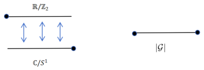${\mathbb{Z}}_2$-action on $\mathbb{R}$ and an $S^1$-action on $\mathbb{C}$.Explicitly, let A and $A^{-1}$ be the sets

$$\begin{array}{cc}\hfill A=& \{(x,z)\in G_0\times G_0|x\in \mathbb{R},z\in \mathbb{C},x\ne 0,|z|={\displaystyle \frac{1}{|x|}}\}\hfill \\ \hfill A^{-1}=& \{(z,x)\in G_0\times G_0|x\in \mathbb{R},z\in \mathbb{C},x\ne 0,|z|={\displaystyle \frac{1}{|x|}}\}.\hfill \end{array}$$

Let

$$G_1=({\mathbb{Z}}_2\times \mathbb{R})\bigsqcup (S^1\times \mathbb{C})\bigsqcup A\bigsqcup A^{-1}$$

and define the source and target maps by

$$\begin{array}{cccccc}\hfill & s\left(\right(g,x\left)\right)=x,\hfill & \hfill & t\left(\right(g,x\left)\right)=gx,\hfill & \hfill & \mathit{for}(g,x)\in {\mathbb{Z}}_2\times \mathbb{R}\hfill \\ \hfill & s\left((e^{i\theta },z)\right)=z,\hfill & \hfill & t\left((e^{i\theta },z)\right)=e^{i\theta }z,\hfill & \hfill & \mathit{for}(e^{i\theta },z)\in S^1\times \mathbb{C}\hfill \\ \hfill & s\left(\right(x,z\left)\right)=x,\hfill & \hfill & t\left(\right(x,z\left)\right)=z,\hfill & \hfill & \mathit{for}(x,z)\in A\hfill \\ \hfill & s\left(\right(z,x\left)\right)=z,\hfill & \hfill & t\left(\right(z,x\left)\right)=x,\hfill & \hfill & \mathit{for}(z,x)\in A^{-1},\hfill \end{array}$$

We can verify that the definition satisfies the groupoid axioms.

Note that the arrows ${\mathbb{Z}}_2\times \mathbb{R}$ and $S^1\times \mathbb{C}$ are the arrows from the action groupoids, hence satisfy the composition associativity, unit and inverse groupoid axioms.

For the glueing arrows A and $A^{-1}$, if $g,h\in A\cup A^{-1}$, $t\left(g\right)=s\left(h\right)$, then by the source and target map, $g\in A$, $h\in A^{-1}$ or $g\in A^{-1}$, $h\in A$.

When $g\in A$ and $h\in A^{-1}$ with $t\left(g\right)=s\left(h\right)$, by definition of A and $A^{-1}$, $\left|x\right|=\left|y\right|\in \mathbb{R}$. Let $y=\alpha x$ for $\alpha =1$ or $-1$, then $hg=(\alpha ,x)in{\mathbb{Z}}_2\times \mathbb{R}$. In addition, $hg\left(x\right)=y=h\left(z\right)=h\left(g\right(x\left)\right)$. Also $s\left(hg\right)=s\left(g\right)$, $t(h\circ g)=t\left(h\right)$. Therefore, the composition and associativity axioms are satisfied. By the same argument, if $g\in A^{-1}$ and $h\in A$ with $t\left(g\right)=s\left(h\right)$, then $hg\in S^1\times \mathbb{C}$. In addition, $hg\left(z\right)=x=h\left(x\right)=h\left(g\right(z\left)\right)$. Also $s\left(hg\right)=s\left(g\right)$, $t(h\circ g)=t\left(h\right)$. Therefore, the composition and associativity axioms are satisfied. Since unit arrows and inverse clearly exist, then $\mathcal{G}:G_1\rightrightarrows G_0$ is a groupoid.

Let

$$\pi :G_0=\mathbb{R}\bigsqcup \mathbb{C}⟶\left|\mathcal{G}\right|$$

be the orbit projection. There are three types of points in $|\mathcal{G}|$, and their local linearized charts can be described explicitly as follows.

1.

Let $x_0=0\in \mathbb{R}$. For $0<\epsilon <1$, set

$${\tilde{U}}_{x_0}=(-\epsilon ,\epsilon )\bigsqcup \{z\in \mathbb{C}:|z|>{\epsilon }^{-1}\},U_{x_0}=\pi \left({\tilde{U}}_{x_0}\right).$$

Then,

$${\mathcal{G}|}_{U_{x_0}}\simeq {\mathbb{Z}}_2⋉(-\epsilon ,\epsilon ),$$

where ${\mathbb{Z}}_2$ acts by $x\mapsto -x$. Thus, $(U_{x_0},{\Psi }_{x_0})$ is a local linearized chart at $\pi \left(x_0\right)$.

2.

Let $x\in \mathbb{R}\setminus \left\{0\right\}$, and put $r_0=\left|x\right|$. Choose $0<\delta <r_0$ and set $I=(r_0-\delta ,r_0+\delta ).$ The corresponding saturated neighborhood is

$${\tilde{U}}_x={\{r\in \mathbb{R}:|r|\in I\}\bigsqcup \{z\in \mathbb{C}:|z|}^{-1}\in I\}.$$

Then,

$${\mathcal{G}|}_{\pi \left({\tilde{U}}_x\right)}\simeq \left\{e\right\}⋉I.$$

Hence, every nonzero orbit has a local linearized chart with trivial isotropy group.

3.

Let $z_0=0\in \mathbb{C}$. For $0<\epsilon <1$, let $D_{\epsilon }=\{z\in \mathbb{C}:|z|<\epsilon \}$ and set

$${\tilde{U}}_{z_0}=\{x\in \mathbb{R}:|x|>{\epsilon }^{-1}\}\bigsqcup D_{\epsilon },U_{z_0}=\pi \left({\tilde{U}}_{z_0}\right).$$

Then,

$${\mathcal{G}|}_{U_{z_0}}\simeq S^1⋉D_{\epsilon },$$

where $S^1$ acts on $D_{\epsilon }$ by rotations. Thus, $(U_{z_0},{\Psi }_{z_0})$ is a local linearized chart at $\pi \left(z_0\right)$.

Therefore, $\mathcal{G}$ is locally linearizable.

Remark 3. 

Although the local linearizable groupoid $\mathcal{G}$ is not assumed to be a Lie groupoid globally, every local model appearing in the definition is equivalent to an action Lie groupoid by a chart. Differential geometric constructions are performed on these local action Lie groupoid charts.

Recall that let $\mathcal{G}:G_1\rightrightarrows G_0$ be a local linearizable groupoid and let $X=\left|\mathcal{G}\right|$ be its orbit space. A local linearized chart on an open subset $U\subset X$ consists of a local model

$${\Psi }_U{:\mathcal{G}|}_U⟶G_U⋉S_U,$$

where $G_U$ is a compact Lie group and $S_U$ is a smooth $G_U$-manifold.

Definition 4. 

We say that a collection

$${\left\{(U,{\Psi }_U)\right\}}_{U\in \mathcal{B}}$$

of local linearized charts is compatible if the following conditions are satisfied.

1.

The collection $\mathcal{B}$ of chart domains forms a basis for the topology of X. In particular, for every open subset $O\subset X$ and every point $y\in O$, there exists $U\in \mathcal{B}$ such that

$$y\in U\subset O.$$

2.

Let $(U,{\Psi }_U)$, and $(V,{\Psi }_V)$ be two local linearized charts and let $y\in U\cap V.$ Then there exists a local linearized chart $(W,{\Psi }_W)$ with $y\in W\subset U\cap V,$ together with embeddings of action groupoids

$${\lambda }_{W,U}:G_W⋉S_W⟶G_U⋉S_U$$

and

$${\lambda }_{W,V}:G_W⋉S_W⟶G_V⋉S_V.$$

Each such embedding is induced by an equivariant pair

$$({𝚥}_{W,U},i_{W,U}):(G_W,S_W)⟶(G_U,S_U)$$

and, respectively,

$$({𝚥}_{W,V},i_{W,V}):(G_W,S_W)⟶(G_V,S_V),$$

where

$${𝚥}_{W,U}:G_W⟶G_U,{𝚥}_{W,V}:G_W⟶G_V$$

are Lie group homomorphisms and

$$i_{W,U}:S_W⟶S_U,i_{W,V}:S_W⟶S_V$$

are equivariant smooth embeddings. Let

$$q_U:S_U⟶S_U/G_U\simeq U,$$

$$q_V:S_V⟶S_V/G_V\simeq V,$$

and

$$q_W:S_W⟶S_W/G_W\simeq W$$

be the quotient maps. The embeddings are required to induce the ordinary inclusions on the orbit spaces:

$$q_U\circ i_{W,U}={\iota }_{W,U}\circ q_W$$

$$q_V\circ i_{W,V}={\iota }_{W,V}\circ q_W,$$

where

$${\iota }_{W,U}:W\hookrightarrow U,{\iota }_{W,V}:W\hookrightarrow V$$

are the inclusion maps.

3.

Refinement embeddings are compatible with composition. More precisely, suppose $W\subset V\subset U$ are chart domains and refinement embeddings

$${\lambda }_{W,V}:G_W⋉S_W⟶G_V⋉S_V$$

$${\lambda }_{V,U}:G_V⋉S_V⟶G_U⋉S_U$$

are given. Then, their composition

$${\lambda }_{V,U}\circ {\lambda }_{W,V}:G_W⋉S_W⟶G_U⋉S_U$$

is again an admissible refinement embedding. Equivalently, for the corresponding equivariant pairs,

$${𝚥}_{W,U}={𝚥}_{V,U}\circ {𝚥}_{W,V},$$

$$i_{W,U}=i_{V,U}\circ i_{W,V}$$

whenever ${\lambda }_{W,U}$ is defined to be this composite.

4.

The refinement embeddings are locally coherent in the sense of germs. Namely, suppose that two refinement embeddings are given after possibly different refinements:

$${\lambda }_{V_1,U}:G_{V_1}⋉S_{V_1}\to G_U⋉S_U,$$

and

$${\lambda }_{V_2,U}:G_{V_2}⋉S_{V_2}\to G_U⋉S_U,$$

where $V_1\subset U$, $V_2\subset U$ and $y\in V_1\cap V_2$. Then there exists a further refinement

$$W\subset V_1\cap V_2$$

such that the two induced refinements from W to U coincide.

A groupoid equipped with such a compatible system of local linearized charts will be called a slice groupoid.

Remark 4. 

The compatibility condition above is local. It does not require a specified comparison morphism for every inclusion of chart domains $V\subset U.$ Instead, it requires that comparison morphisms exist after passing to sufficiently small neighborhoods and that different choices become equal after a further refinement.

This is precisely the amount of compatibility needed to define germs of local Cartan elements.

Recall that when M is a manifold with a proper action of a compact Lie group G, the slice theorem gives, for every $y\in M/G$ and every $x\in {\pi }^{-1}\left(y\right)$,

$$\tilde{U}\simeq G{ \times }_{G_x}{S}_x,$$

where $\tilde{U}\subset M$ is a G-invariant neighborhood of the orbit ${\pi }^{-1}\left(y\right)$. We use the right $G_x$-action on $G\times S_x$ and the left G-action on $G{ \times }_{G_x}{S}_x$ given by

$$(g,p)·h=(gh,h^{-1}·p)$$

and

$$k·[g,q]=[kg,q].$$

Theorem 4. 

The action groupoids $G_x⋉S_x$ and $G⋉\left(G{ \times }_{G_x}{S}_x\right)$ are equivalent. In particular, they are Morita equivalent.

Proof. 

Define

$$\Phi :G_x⋉S_x⟶G⋉\left(G{ \times }_{G_x}{S}_x\right)$$

by

$$\begin{array}{cc}\hfill {\Phi }_0:S_x& ⟶G{ \times }_{G_x}{S}_x\hfill \\ \hfill s& \mapsto [e,s]\hfill \end{array}$$

and

$$\begin{array}{cc}\hfill {\Phi }_1:G_x\times S_x& ⟶G\times \left(G{ \times }_{G_x}{S}_x\right)\hfill \\ \hfill (h,s)& \mapsto (h,[e,s\left]\right).\hfill \end{array}$$

Then,

$$s\left({\Phi }_1(h,s)\right)=[e,s]={\Phi }_0\left(s\right),$$

while

$$t\left({\Phi }_1(h,s)\right)=h·[e,s]=[h,s].$$

Since

$$[h,s]=[e,h·s],$$

we obtain

$$t\left({\Phi }_1(h,s)\right)=[e,h·s]={\Phi }_0(h·s).$$

Thus, $\Phi$ is a well-defined morphism of action groupoids.

Next, we verify that $\Phi$ is an equivalence. Firstly, consider the map

$$t\circ {\mathrm{pr}}_1:{\left(G\times \left(G{ \times }_{G_x}{S}_x\right)\right)}_s{ \times }_{{\Phi }_0}{S}_x⟶G{ \times }_{G_x}{S}_x,$$

where

$${\left(G\times \left(G{ \times }_{G_x}{S}_x\right)\right)}_s{ \times }_{{\Phi }_0}{S}_x=\left\{\left((g,[e,s\left]\right),s\right)|g\in G,s\in S_x\right\}.$$

This fiber product is naturally diffeomorphic to $G\times S_x$ via

$$\begin{array}{cc}\hfill G\times S_x& ⟶{\left(G\times \left(G{ \times }_{G_x}{S}_x\right)\right)}_s{ \times }_{{\Phi }_0}{S}_x\hfill \\ \hfill (g,s)& ⟼\left((g,[e,s\left]\right),s\right).\hfill \end{array}$$

Under this identification, the map $t\circ {\mathrm{pr}}_1$ becomes

$$q:G\times S_x⟶G{ \times }_{G_x}{S}_x,q(g,s)=[g,s].$$

The map q is the quotient map of the free and proper right $G_x$-action

$$(g,s)·h=(gh,h^{-1}s).$$

Hence, q is a surjective submersion. Therefore the first condition for equivalence is satisfied.

It remains to verify full faithfulness. Consider the fiber product

$${(S_x\times S_x)}_{{\Phi }_0\times {\Phi }_0}{ \times }_{(s,t)}\left(G\times \left(G{ \times }_{G_x}{S}_x\right)\right).$$

An element of this fiber product is a triple $(s_1,s_2,g)$ such that

$$[e,s_1]=s(g,[e,s_1])$$

and

$$g·[e,s_1]=[e,s_2].$$

Thus, the condition is precisely

$$[g,s_1]=[e,s_2].$$

By the definition of the quotient $G{ \times }_{G_x}{S}_x$, this equality holds if and only if there exists $h\in G_x$ such that

$$g=h\mathit{and}{s}_2=h·s_1.$$

Indeed,

$$[g,s_1]=[e,s_2]$$

means that for some $h\in G_x$,

$$(g,s_1)·h=(e,s_2),$$

that is,

$$gh=e,h^{-1}{s}_1=s_2.$$

Equivalently, with $k=h^{-1}\in G_x$,

$$g=k,s_2=k·s_1.$$

Hence, the map

$$G_x\times S_x⟶{(S_x\times S_x)}_{{\Phi }_0\times {\Phi }_0}{ \times }_{(s,t)}\left(G\times \left(G{ \times }_{G_x}{S}_x\right)\right),$$

defined by

$$(h,s)⟼\left(s,h·s,h\right),$$

is a diffeomorphism. Under this identification, the canonical map from the arrow space of $G_x⋉S_x$ to the above fiber product is exactly this diffeomorphism.

Therefore $\Phi$ is fully faithful and essentially surjective. Hence, $G_x⋉S_x$ and $G⋉\left(G{ \times }_{G_x}{S}_x\right)$ are equivalent groupoids. Consequently, they are Morita equivalent. □

Example 5. 

An action groupoid $G⋉M$ with a proper G-action is a slice groupoid. One may also construct another slice groupoid that encodes the slice data. Explicitly, let ${\left\{U_{\alpha }\right\}}_{\alpha }$ be an open cover of the orbit space $|G⋉M|$ such that the slice theorem holds for each $U_{\alpha }$. We take a slice $S_{\alpha }$ in M and define

$$G_0=\underset{\alpha }{⨆}{S}_{\alpha },$$

then we have a natural inclusion

$$i:G_0\to M.$$

Let

$$G_1=\{(p,q,g)\in G_0\times G_0 \times G|g·i\left(p\right)=i\left(q\right)\},$$

and define the source and target maps by

$$\begin{array}{cc}\hfill s(p,q,g)& =p\hfill \\ \hfill t(p,q,g)& =q.\hfill \end{array}$$

Then, the local charts define a slice groupoid $G_1\rightrightarrows G_0$.

Example 6. 

Orbifold groupoids are slice groupoids because an orbifold is locally modeled by an action groupoid $G⋉{\mathbb{R}}^n$ for a finite group G.

We give one more example of a slice groupoid whose orbit space is not a global quotient.

Example 7. 

Let $U=D/Z_m$ be a topological space, where D is the open unit disk in $\mathbb{C}\simeq {\mathbb{R}}^2$ and ${\mathbb{Z}}_m$ is a finite group whose generator τ acts on D by

$$\tau ·z=e^{i{\displaystyle \frac{2\pi }{m}}}z.$$

Let $V=(D\times S^1)/S^1$ where $S^1$ acts on $D\times S^1$ by

$$e^{i\theta }·(z,e^{i\lambda })=(e^{i\theta }z,e^{i\lambda }).$$

The orbit space $|\mathcal{G}|$ is given by gluing U and V as follows

$$|\mathcal{G}|=(U\bigsqcup V)/\sim$$

where $x\in U$, $y\in V$ are equivalent if

$$\begin{array}{cc}\hfill x=& \left[r{e}^{i\lambda }\right],r\ne 0\hfill \\ \hfill y=& [(1-r)e^{i2\pi },e^{im\lambda }].\hfill \end{array}$$

The following figure illustrates how U and V are glued together.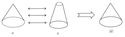

Explicitly, let $\mathcal{G}=G_1\rightrightarrows G_0$ be a groupoid, where

$$G_0=D\bigsqcup (D\times S^1)$$

and

$$\begin{array}{cc}\hfill G_1=& ({\mathbb{Z}}_m\times D)\bigsqcup \left(S^1\times (D\times S^1)\right)\hfill \\ \hfill & \bigsqcup \{(x,y)\in D\times (D\times S^1)|x=r{e}^{i\theta },y=(z,e^{im\theta }),0<r<1,|z|=1-r\}\hfill \\ \hfill & \bigsqcup \{(y,x)\in (D\times S^1)\times D|x=r{e}^{i\theta },y=(z,e^{im\theta }),0<r<1,|z|=1-r\}\hfill \end{array}$$

where the source and target maps on the action-groupoid components generate the group actions on $G_0$, while the source and target maps on the remaining two components generate the gluing arrows and their inverses.

In this example, there are three types of points in $\left|\mathcal{G}\right|$:

• If $p=[0,\theta ]\in V\subset \left|\mathcal{G}\right|$, there is a neighborhood $V_p^{\prime }\subset \left|\mathcal{G}\right|$ of p such that ${\mathcal{G}|}_{V_p^{\prime }}$ is Morita equivalent to $S^1⋉\left(D_{\delta }\times (\theta -ϵ,\theta +ϵ)\right)$, where $D_{\delta }$ is a disk with radius δ, ϵ is a small real number greater than zero, and $S^1$ acts on $D_{\delta }$ by rotation.
• If $q=\left[0\right]\in U\subset \left|\mathcal{G}\right|$, there is a neighborhood $U_q^{\prime }\subset \left|\mathcal{G}\right|$ of q such that ${\mathcal{G}|}_{U_q^{\prime }}$ is Morita equivalent to ${\mathbb{Z}}_m⋉D_{\delta }$.
• The other points are smooth points, i.e., there is a neighborhood $W^{\prime }$ of each point such that ${\mathcal{G}|}_{W^{\prime }}$ is Morita equivalent to $\left\{e\right\}⋉D_{\delta }$. where $\left\{e\right\}$ is the trivial group.

Therefore, for any point in $\left|\mathcal{G}\right|$, there exists a neighborhood that is locally modeled on the quotient of a slice by a compact Lie group action.

This example illustrates that slice groupoids encompass spaces that are not global quotients, thereby generalizing the framework of orbifolds and proper Lie group actions.

4. Equivariant Cohomology on Slice Groupoids

4.1. Sheaf-Theoretic Preliminaries

We briefly recall the sheaf-theoretic notation and standard facts that will be used in the sequel. For general background on sheaves, complexes of sheaves, and hypercohomology, we refer to [19,20,21].

Let $\mathcal{F}$ be a sheaf on a topological space X. For $x\in X$, we denote by ${\mathcal{F}}_x$ the stalk of $\mathcal{F}$ at x, and by ${\left[s\right]}_x$ the germ at x of a local section s. If ${\mathcal{F}}^{\prime }$ is a presheaf, its sheafification has the same stalks as ${\mathcal{F}}^{\prime }$. We shall also use the standard étalé-space realization of a sheaf: the disjoint union

$$\coprod _{x\in X}{\mathcal{F}}_x$$

of its stalks is endowed with the usual topology for which local sections of $\mathcal{F}$ correspond to continuous sections of the projection onto X; see [20].

Let ${\mathcal{F}}^{•}$ be a complex of sheaves on X. Its q-th cohomology sheaf is denoted by ${\mathcal{H}}^q\left({\mathcal{F}}^{•}\right),$ and its stalk at x is naturally identified with the cohomology of the stalk complex:

$${\mathcal{H}}^q{\left({\mathcal{F}}^{•}\right)}_x\cong H^q\left({\mathcal{F}}_x^{•}\right).$$

A morphism of complexes of sheaves

$$\varphi :{\mathcal{F}}^{•}⟶{\mathcal{G}}^{•}$$

is called a quasi-isomorphism if it induces an isomorphism

$${\mathcal{H}}^q\left({\mathcal{F}}^{•}\right)⟶{\mathcal{H}}^q\left({\mathcal{G}}^{•}\right)$$

for every q.

For a bounded-below complex of sheaves ${\mathcal{F}}^{•}$, we denote its hypercohomology by

$${\mathbb{H}}^q(X;{\mathcal{F}}^{•}).$$

A quasi-isomorphism of bounded-below complexes of sheaves induces an isomorphism on hypercohomology. Moreover, if each sheaf ${\mathcal{F}}^q$ is acyclic for the global-section functor, then

$${\mathbb{H}}^{\ast }(X;{\mathcal{F}}^{•})\cong H^{\ast }\left(\Gamma (X,{\mathcal{F}}^{•})\right).$$

Finally, on a paracompact Hausdorff space, fine sheaves are soft and soft sheaves are acyclic (see, for example [20]). Consequently, a bounded-below complex whose terms are fine has hypercohomology computed by its complex of global sections.

4.2. Equivariant Cohomology of Slice Groupoids

We apply the preceding sheaf-theoretic results to generalize equivariant cohomology to slice groupoids.

Theorem 5 

(Morita invariance for action groupoids). Let

$$\mathcal{H}=H⋉N,\mathcal{G}=G⋉M$$

be action Lie groupoids, where H and G are compact Lie groups. If $\mathcal{H}$ and $\mathcal{G}$ are equivalent Lie groupoids, then there is a canonical isomorphism

$$H_H^{\ast }(N;\mathbb{R})\cong H_G^{\ast }(M;\mathbb{R}).$$

More generally, the same conclusion holds if $\mathcal{H}$ and $\mathcal{G}$ are Morita equivalent.

Proof. 

Recall that the classifying space of an action groupoid is naturally homotopy equivalent to the corresponding Borel construction:

$$B(H⋉N)\simeq E_H{ \times }_{H}N,$$

and

$$B(G⋉M)\simeq E_G{ \times }_{G}M.$$

A groupoid equivalence induces a weak homotopy equivalence between classifying spaces [14]. Hence, an equivalence

$$\mathcal{H}⟶\mathcal{G}$$

induces a weak homotopy equivalence

$$B\mathcal{H}\simeq B\mathcal{G}.$$

The same conclusion holds for a Morita equivalence, since a span of groupoid equivalences

$$\mathcal{H}⟵\mathcal{K}⟶\mathcal{G}$$

induces weak homotopy equivalences

$$B\mathcal{H}\simeq B\mathcal{K}\simeq B\mathcal{G}.$$

Therefore,

$$H^{\ast }(E_H{ \times }_{H}N;\mathbb{R})\cong H^{\ast }(E_G{ \times }_{G}M;\mathbb{R}).$$

By the definition of equivariant cohomology,

$$H_H^{\ast }(N;\mathbb{R})=H^{\ast }(E_H{ \times }_{H}N;\mathbb{R})$$

and

$$H_G^{\ast }(M;\mathbb{R})=H^{\ast }(E_G{ \times }_{G}M;\mathbb{R}).$$

Thus

$$H_H^{\ast }(N;\mathbb{R})\cong H_G^{\ast }(M;\mathbb{R}).$$

□

4.3. The Cartan Sheaf of a Slice Groupoid

Let

$$\mathcal{G}:G_1\rightrightarrows G_0$$

be a slice groupoid and let $X=\left|\mathcal{G}\right|$ be its orbit space. Fix a compatible system of local linearized charts ${\left\{(U,{\Psi }_U)\right\}}_{U\in \mathcal{B}}$ as in Definition 4.

For every $U\in \mathcal{B},$ write

$${\Psi }_U{:\mathcal{G}|}_U⟶G_U⋉S_U,$$

and associate to the chart the Cartan complex

$${\mathcal{A}}^{•}\left(U\right):=\mathrm{Car}(S_U,G_U).$$

We emphasize that no restriction morphism

$${\mathcal{A}}^{•}\left(U\right)⟶{\mathcal{A}}^{•}\left(V\right)$$

is assumed to exist for every inclusion $V\subset U.$ Instead, restriction morphisms are defined only when a compatible refinement embedding of the corresponding local models is available.

Suppose that $V\subset U$ are chart domains and that there is a refinement embedding

$${\lambda }_{V,U}:G_V⋉S_V⟶G_U⋉S_U.$$

Write the corresponding equivariant pair as

$$({𝚥}_{V,U},i_{V,U}):(G_V,S_V)⟶(G_U,S_U).$$

Thus,

$${𝚥}_{V,U}:G_V⟶G_U$$

is a Lie group homomorphism and

$$i_{V,U}:S_V⟶S_U$$

is a ${𝚥}_{V,U}$-equivariant smooth embedding.

The refinement embedding determines a Cartan morphism

$${\rho }_{U,V}:\mathrm{Car}(S_U,G_U)⟶\mathrm{Car}(S_V,G_V)$$

defined by

$$\left({\rho }_{U,V}\alpha \right)\left(\eta \right)=i_{V,U}^{\ast }\left(\alpha \left(d{𝚥}_{V,U}\left(\eta \right)\right)\right),\eta \in {\mathfrak{g}}_V.$$

(21)

By Proposition 2, the equivariant pair

$$({𝚥}_{V,U},i_{V,U}):(G_V,S_V)⟶(G_U,S_U)$$

induces a morphism of differential graded algebras

$${\rho }_{U,V}:\mathrm{Car}(S_U,G_U)⟶\mathrm{Car}(S_V,G_V).$$

In particular,

$$D_{C,V}\circ {\rho }_{U,V}={\rho }_{U,V}\circ D_{C,U}.$$

We now organize these local Cartan complexes pointwise.

Definition 5. 

Let $y\in X.$ The category ${\mathcal{N}}_y$ is defined as follows. Its objects are the local linearized charts $(U,{\Psi }_U)$ such that $y\in U.$ A morphism

$$U⟶V$$

in ${\mathcal{N}}_y$ is represented by a refinement

$$y\in V\subset U$$

together with a refinement embedding

$${\lambda }_{V,U}:G_V⋉S_V⟶G_U⋉S_U.$$

The direction of the morphism is chosen so that the associated Cartan morphism has the same direction:

$${\rho }_{U,V}:\mathrm{Car}(S_U,G_U)⟶\mathrm{Car}(S_V,G_V).$$

Two refinement morphisms are identified if they agree after passing to a further chart neighborhood of y.

Composition is induced by composition of refinement embeddings.

Proposition 6. 

For every $y\in X,$ the category ${\mathcal{N}}_y$ is filtered.

Proof. 

The category is nonempty because the local linearized chart domains form a basis of the topology of X.

Let $U\mathrm{and}V\in {\mathcal{N}}_y.$ By compatibility of the local linearized charts, there exists $W\in \mathcal{B}$ such that

$$y\in W\subset U\cap V$$

and there are refinement embeddings

$$G_W⋉S_W⟶G_U⋉S_U$$

and

$$G_W⋉S_W⟶G_V⋉S_V.$$

Thus, there are morphisms

$$U⟶W\mathrm{and}V⟶W$$

in ${\mathcal{N}}_y$.

Suppose now that two parallel refinement morphisms are given. By the local coherence condition in Definition 4, after passing to a sufficiently small chart neighborhood $W\ni y,$ the two induced refinement morphisms agree. Hence the two parallel morphisms are equalized after a further refinement. Therefore, ${\mathcal{N}}_y$ is filtered. □

The Cartan complexes and the admissible refinement morphisms define a functor

$${\mathcal{A}}_y^{•}:{\mathcal{N}}_y⟶{\mathbf{CDGA}}_{\mathbb{R}},$$

given on objects by

$$U⟼\mathrm{Car}(S_U,G_U)$$

and on morphisms by

$$U⟶V⟼{\rho }_{U,V}.$$

Definition 6 

(Cartan stalk). For $y\in X,$ define the Cartan stalk of the slice groupoid at y by the filtered direct limit

$${\mathcal{C}}_{\mathcal{G},y}^{•}:=\underset{U\in {\mathcal{N}}_y}{\underrightarrow{lim}}\mathrm{Car}(S_U,G_U).$$

(22)

An element of ${\mathcal{C}}_{\mathcal{G},y}^{•}$ will be called a Cartan germ at y.

More explicitly, a representative of a Cartan germ at y is a pair $(U,\alpha ),$ where $y\in U\in \mathcal{B}$ and $\alpha \in \mathrm{Car}(S_U,G_U).$ Two representatives $(U,\alpha )\mathit{and}(V,\beta )$ represent the same germ at y if there exists a common refinement

$$y\in W\subset U\cap V$$

with refinement morphisms

$${\rho }_{U,W}:\mathrm{Car}(S_U,G_U)⟶\mathrm{Car}(S_W,G_W)$$

and

$${\rho }_{V,W}:\mathrm{Car}(S_V,G_V)⟶\mathrm{Car}(S_W,G_W)$$

such that

$${\rho }_{U,W}\left(\alpha \right)={\rho }_{V,W}\left(\beta \right).$$

The equivalence class of $(U,\alpha )$ is denoted by ${\left[\alpha \right]}_{y,U},$ or simply by ${\left[\alpha \right]}_y.$ Because the category ${\mathcal{N}}_y$ is filtered, this relation is an equivalence relation.

Since every refinement morphism commutes with the Cartan differential, the differential passes to the filtered direct limit:

$$D_C:{\mathcal{C}}_{\mathcal{G},y}^k⟶{\mathcal{C}}_{\mathcal{G},y}^{k+1},$$

with

$$D_C{\left[\alpha \right]}_y={\left[D_C\alpha \right]}_y.$$

The product also passes to the direct limit. Hence, ${\mathcal{C}}_{\mathcal{G},y}^{•}$ is a differential graded algebra.

We now construct the associated étalé space. For every degree k, set

$$E_{\mathcal{G}}^k=\underset{y\in X}{⨆}{\mathcal{C}}_{\mathcal{G},y}^k$$

and define

$$p^k:E_{\mathcal{G}}^k⟶X$$

by

$$p^k\left({\left[\alpha \right]}_y\right)=y.$$

Let $U\in \mathcal{B}$ and $\alpha \in {\mathrm{Car}}^k(S_U,G_U).$ Define

$$\widehat{\alpha }:U⟶E_{\mathcal{G}}^k$$

by

$$\widehat{\alpha }\left(y\right)={\left[\alpha \right]}_y.$$

(23)

We give $E_{\mathcal{G}}^k$ the topology generated by the subsets

$$\widehat{\alpha }\left(U\right)=\left\{{\left[\alpha \right]}_y\mid y\in U\right\},$$

where $U\in \mathcal{B}$ and $\alpha \in {\mathrm{Car}}^k(S_U,G_U).$ The common-refinement property implies that these subsets form a basis for a topology. Indeed, if

$${\left[\alpha \right]}_y={\left[\beta \right]}_y,$$

then, by the definition of equality of germs, there exists a common refinement $y\in W$ on which the two representatives agree. Consequently,

$$\widehat{\alpha }\left(W\right)=\widehat{\beta }\left(W\right).$$

With this topology,

$$p^k:E_{\mathcal{G}}^k⟶X$$

is a local homeomorphism.

Definition 7 

(Cartan sheaf of a slice groupoid). For every open subset $O\subset X,$ define ${\mathcal{C}}_{\mathcal{G}}^k\left(O\right)$ to be the space of continuous sections of the espace étalé

$$p^k:E_{\mathcal{G}}^k⟶X$$

over O:

$${\mathcal{C}}_{\mathcal{G}}^k\left(O\right)=\left\{s:O⟶E_{\mathcal{G}}^k|p^k\circ s={\mathrm{id}}_O,s\mathit{is}\mathit{continuous}\right\}.$$

If $V\subset O$ are arbitrary open subsets of X, define the restriction morphism by ordinary restriction of sections:

$${\rho }_{O,V}:{\mathcal{C}}_{\mathcal{G}}^k\left(O\right)⟶{\mathcal{C}}_{\mathcal{G}}^k\left(V\right),$$

$${\rho }_{O,V}{\left(s\right)=s|}_V.$$

Thus, the restriction morphism is now defined for every inclusion $V\subset O$ and does not require a comparison map between slice charts.

The stalkwise Cartan differential defines

$$D_C:{\mathcal{C}}_{\mathcal{G}}^k⟶{\mathcal{C}}_{\mathcal{G}}^{k+1}$$

by

$$\left(D_{C}s\right)\left(y\right)=D_C\left(s\left(y\right)\right).$$

Since every section is locally represented by an element of a local Cartan complex, the section $D_{C}s$ is again continuous. Therefore, $({\mathcal{C}}_{\mathcal{G}}^{•},D_C)$ is a complex of sheaves. The product is defined stalkwise, and hence ${\mathcal{C}}_{\mathcal{G}}^{•}$ is a sheaf of differential graded algebras.

By construction, the stalk of this sheaf at

$$y\in X$$

is naturally identified with the filtered direct limit

$${({\mathcal{C}}_{\mathcal{G}}^{•})}_y\cong {\mathcal{C}}_{\mathcal{G},y}^{•}=\underset{U\in {\mathcal{N}}_y}{\underrightarrow{lim}}\mathrm{Car}(S_U,G_U).$$

For every chart domain

$$U\in \mathcal{B},$$

there is a natural morphism

$$\mathrm{Car}(S_U,G_U)⟶\Gamma \left(U,{\mathcal{C}}_{\mathcal{G}}^{•}\right)$$

given by

$$\alpha ⟼\widehat{\alpha },$$

where

$$\widehat{\alpha }\left(y\right)={\left[\alpha \right]}_y.$$

Definition 8. 

The Cartan complex of the slice groupoid $\mathcal{G}$ is the complex of global sections

$$\mathrm{Car}\left(\mathcal{G}\right):=\Gamma \left(X,{\mathcal{C}}_{\mathcal{G}}^{•}\right).$$

The equivariant cohomology of $\mathcal{G}$ is defined by

$$H_{\mathcal{G}}^{\ast }(\mathcal{G};\mathbb{R}):=H^{\ast }\left(\mathrm{Car}\left(\mathcal{G}\right),D_C\right).$$

Now let G be a compact Lie group acting smoothly and properly on a manifold M, and let

$$\pi :M⟶X=M/G$$

be the quotient map. For every open subset $U\subset X$, define

$${\mathcal{C}}_{G,M}^{•}\left(U\right)=\mathrm{Car}({\pi }^{-1}\left(U\right),G).$$

The usual restriction of differential forms defines the restriction maps. Hence,

$$U⟼\mathrm{Car}({\pi }^{-1}\left(U\right),G)$$

is a sheaf of complexes on X, which we call the ordinary Cartan sheaf of the G-manifold M. Its global sections are

$$\Gamma \left(X,{\mathcal{C}}_{G,M}^{•}\right)=\mathrm{Car}(M,G).$$

Proposition 7. 

Let G be a compact Lie group acting smoothly and properly on M, and let

$$X=M/G.$$

Let $\mathcal{G}$ be a slice groupoid representation of the action groupoid $G⋉M$, constructed from a compatible system of local linearized charts in the sense of Definition 4.

Then, the local Cartan reduction morphisms define a morphism of complexes of sheaves

$$\mathcal{R}:{\mathcal{C}}_{G,M}^{•}⟶{\mathcal{C}}_{\mathcal{G}}^{•}.$$

Moreover, $\mathcal{R}$ is a quasi-isomorphism of complexes of sheaves.

Proof. 

We first construct the morphism of sheaves. Let $O\subset X$ be open and let

$$\alpha \in {\mathcal{C}}_{G,M}^{•}\left(O\right)=\mathrm{Car}({\pi }^{-1}\left(O\right),G).$$

For every point $y\in O,$ choose a chart domain $U\in \mathcal{B}$ such that $y\in U\subset O.$ For the slice-groupoid representation associated with the G-action, the chart over U is represented by a slice model $G_U⋉S_U.$ The slice reduction theorem gives a chain map

$${\mathcal{R}}_U:\mathrm{Car}({\pi }^{-1}\left(U\right),G)⟶\mathrm{Car}(S_U,G_U).$$

Define $\left({\mathcal{R}}_O\alpha \right)\left(y\right)$ to be the germ represented by ${\mathcal{R}}_U\left({\alpha |}_{{\pi }^{-1}\left(U\right)}\right).$ Thus,

$$\left({\mathcal{R}}_O\alpha \right)\left(y\right)={\left[{\mathcal{R}}_U\left({\alpha |}_{{\pi }^{-1}\left(U\right)}\right)\right]}_y.$$

(24)

We must show that this definition is independent of the chosen chart U. Suppose $U,V\in \mathcal{B}$ both contain y and are contained in O. By the compatibility of the local linearized charts, there exists a common refinement

$$y\in W\subset U\cap V$$

together with refinement embeddings from the model over W to the models over U and V.

Denote the restriction map of both complex by $\rho$ when there is no ambiguity. Naturality of the Cartan reduction morphism gives

$${\rho }_{U,W}\circ {\mathcal{R}}_U={\mathcal{R}}_W\circ {\rho }_{U,W}$$

and

$${\rho }_{V,W}\circ {\mathcal{R}}_V={\mathcal{R}}_W\circ {\rho }_{V,W}.$$

Therefore,

$${\rho }_{U,W}\left({\mathcal{R}}_U\left(\alpha {|}_{{\pi }^{-1}\left(U\right)}\right)\right)={\mathcal{R}}_W\left(\alpha {|}_{{\pi }^{-1}\left(W\right)}\right)$$

and

$${\rho }_{V,W}\left({\mathcal{R}}_V\left(\alpha {|}_{{\pi }^{-1}\left(V\right)}\right)\right)={\mathcal{R}}_W\left(\alpha {|}_{{\pi }^{-1}\left(W\right)}\right).$$

Hence, the two representatives determine the same germ at y. Thus, $\left({\mathcal{R}}_O\alpha \right)\left(y\right)$ is well defined.

Moreover, let $y\in O$. Choose a sufficiently small chart domain $U\in \mathcal{B}$ such that $y\in U\subset O$, and set

$${\beta }_U={\mathcal{R}}_U\left({\alpha |}_{{\pi }^{-1}\left(U\right)}\right)\in {\mathrm{Car}}^{•}(S_U,G_U).$$

By the definition of ${\mathcal{R}}_O$, for every $z\in U$,

$$\left({\mathcal{R}}_O\alpha \right)\left(z\right)={\left[{\beta }_U\right]}_z.$$

Let

$$\widehat{{\beta }_U}:U⟶E_{\mathcal{G}}^{•},z⟼{\left[{\beta }_U\right]}_z.$$

Then,

$$\left({\mathcal{R}}_O\alpha \right){|}_U=\widehat{{\beta }_U}.$$

Hence,

$$\left({\mathcal{R}}_O\alpha \right){|}_U=\widehat{{\beta }_U}.$$

The topological structure of $E_{\mathcal{G}}^k$ is generated by the basis

$${\mathfrak{B}}_E=\left\{\widehat{\alpha }\left(U\right)|U\in \mathcal{B},\alpha \in {\mathrm{Car}}^k(S_U,G_U)\right\},$$

where

$$\widehat{\alpha }\left(U\right)=\left\{{\left[\alpha \right]}_y|y\in U\right\}.$$

Equivalently, for each

$$U\in \mathcal{B},\alpha \in {\mathrm{Car}}^k(S_U,G_U),$$

the associated map

$$\widehat{\alpha }:U⟶E_{\mathcal{G}}^k,y⟼{\left[\alpha \right]}_y,$$

determines a basic open subset $\widehat{\alpha }\left(U\right)\subset E_{\mathcal{G}}^k$.

By the definition of the étale topology on $E_{\mathcal{G}}^{•}$, the map

$$\widehat{{\beta }_U}:U⟶E_{\mathcal{G}}^{•},z⟼{\left[{\beta }_U\right]}_z,$$

is a continuous local section. Since every point of O admits such a neighborhood U, the section ${\mathcal{R}}_O\alpha$ is continuous on O.

Next we verify that ${\mathcal{R}}_O$ commutes with the restriction maps. Let

$$\alpha \in {\mathcal{C}}_{\mathcal{G},M}^{•}\left(U\right).$$

We prove that

$${\rho }_{U,W}\circ {\mathcal{R}}_U={\mathcal{R}}_W\circ {\rho }_{U,W}.$$

Let $Z\subset W$ be a slice chart. By the definition of the reduction morphism, the restriction of ${\mathcal{R}}_U\left(\alpha \right)$ to Z is

$${\left.{\mathcal{R}}_U\left(\alpha \right)\right|}_Z={\mathrm{Red}}_Z\left({\left.\alpha \right|}_{{\pi }^{-1}\left(Z\right)}\right).$$

On the other hand,

$${\mathcal{R}}_W\left({\rho }_{U,W}\left(\alpha \right)\right)$$

restricted to the same slice chart Z is

$${\mathrm{Red}}_Z\left({\left.\left(\alpha {|}_W\right)\right|}_{{\pi }^{-1}\left(Z\right)}\right).$$

Since $Z\subset W\subset U$, we have

$${\left.\left(\alpha {|}_W\right)\right|}_{{\pi }^{-1}\left(Z\right)}={\left.\alpha \right|}_{{\pi }^{-1}\left(Z\right)}.$$

Therefore, the two expressions coincide on every slice chart $Z\subset W$. Hence, they define the same germ, and consequently

$${\rho }_{U,W}\circ {\mathcal{R}}_U={\mathcal{R}}_W\circ {\rho }_{U,W}.$$

Since the family $\left\{{\mathcal{R}}_U\right\}$ commutes with the restriction maps, the local definitions glue together and define a morphism of sheaves

$$\mathcal{R}:{\mathcal{C}}_{\mathcal{G},M}^{•}⟶{\mathcal{C}}_{\mathcal{G}}^{•},$$

which does not depend on the choice of O.

Moreover, in a sufficiently small slice neighborhood U, the section ${\mathcal{R}}_O\alpha$ is represented by the single Cartan element ${\mathcal{R}}_U\left(\alpha {|}_{{\pi }^{-1}\left(U\right)}\right).$ Therefore, it is a continuous section of the étalé space. Consequently,

$${\mathcal{R}}_O:{\mathcal{C}}_{G,M}^{•}\left(O\right)⟶{\mathcal{C}}_{\mathcal{G}}^{•}\left(O\right)$$

is well defined. If $V\subset O$ is open, the construction immediately gives

$${\rho }_{O,V}\circ {\mathcal{R}}_O={\mathcal{R}}_V\circ {\rho }_{O,V}.$$

Therefore, the morphisms ${\mathcal{R}}_O$ define a morphism of complexes of sheaves

$$\mathcal{R}:{\mathcal{C}}_{G,M}^{•}⟶{\mathcal{C}}_{\mathcal{G}}^{•}.$$

Since each local slice reduction morphism commutes with the Cartan differential, one has

$$D_C\circ \mathcal{R}=\mathcal{R}\circ D_C.$$

It remains to prove that $\mathcal{R}$ is a quasi-isomorphism. Fix $y\in X.$ The stalk of the ordinary Cartan sheaf is

$${\left({\mathcal{C}}_{G,M}^{•}\right)}_y=\underset{y\in O}{\underrightarrow{lim}}\mathrm{Car}({\pi }^{-1}\left(O\right),G).$$

Because the slice-chart domains form a basis for the topology of X, the direct limit may be computed on the cofinal system of slice neighborhoods:

$${\left({\mathcal{C}}_{G,M}^{•}\right)}_y\cong \underset{U\in {\mathcal{N}}_y}{\underrightarrow{lim}}\mathrm{Car}({\pi }^{-1}\left(U\right),G).$$

By construction of the Cartan sheaf of the slice groupoid,

$${\left({\mathcal{C}}_{\mathcal{G}}^{•}\right)}_y\cong \underset{U\in {\mathcal{N}}_y}{\underrightarrow{lim}}\mathrm{Car}(S_U,G_U).$$

The induced morphism on stalks is therefore the filtered direct limit of the local slice reduction morphisms

$${\mathcal{R}}_U:\mathrm{Car}({\pi }^{-1}\left(U\right),G)⟶\mathrm{Car}(S_U,G_U).$$

For every $U\in {\mathcal{N}}_y,$ Theorem 3 implies that ${\mathcal{R}}_U$ is a quasi-isomorphism.

Since ${\mathcal{N}}_y$ is filtered and filtered direct limits of real vector spaces are exact, cohomology commutes with these direct limits. Hence,

$$\begin{array}{cc}\hfill H^q\left({\left({\mathcal{C}}_{G,M}^{•}\right)}_y\right)& \cong \underset{U\in {\mathcal{N}}_y}{\underrightarrow{lim}}{H}^q\left(\mathrm{Car}({\pi }^{-1}\left(U\right),G)\right)\hfill \\ \hfill & \stackrel{\cong }{\to }\underset{U\in {\mathcal{N}}_y}{\underrightarrow{lim}}{H}^q\left(\mathrm{Car}(S_U,G_U)\right)\hfill \\ \hfill & \cong H^q\left({\left({\mathcal{C}}_{\mathcal{G}}^{•}\right)}_y\right).\hfill \end{array}$$

Thus, the induced morphism

$$H^q\left({\left({\mathcal{C}}_{G,M}^{•}\right)}_y\right)⟶H^q\left({\left({\mathcal{C}}_{\mathcal{G}}^{•}\right)}_y\right)$$

is an isomorphism for every q and every $y\in X.$

Therefore,

$$\mathcal{R}:{\mathcal{C}}_{G,M}^{•}⟶{\mathcal{C}}_{\mathcal{G}}^{•}$$

is a quasi-isomorphism of complexes of sheaves. □

Proposition 8. 

Assume that $X=M/G$ is paracompact and that for every locally finite open covering $\left\{U_{\alpha }\right\}$ of X, there exists a subordinate partition of unity $\left\{{\rho }_{\alpha }\right\}$ such that every pullback ${\pi }^{\ast }{\rho }_{\alpha }$ is a smooth G-invariant function on M. Then, for every degree q, the sheaves ${\mathcal{C}}_{G,M}^q\mathit{and}{\mathcal{C}}_{\mathcal{G}}^q$ are fine. In particular, they are acyclic.

Proof. 

Let $\left\{U_{\alpha }\right\}$ be a locally finite open covering of X, and choose a subordinate partition of unity $\left\{{\rho }_{\alpha }\right\}$ as in the hypothesis.

For the ordinary Cartan sheaf, define

$$h_{\alpha }:{\mathcal{C}}_{G,M}^q⟶{\mathcal{C}}_{G,M}^q$$

locally by

$$h_{\alpha }\left(\omega \right)=\left({\pi }^{\ast }{\rho }_{\alpha }\right)\omega .$$

Since ${\pi }^{\ast }{\rho }_{\alpha }$ is smooth and G-invariant, multiplication by ${\pi }^{\ast }{\rho }_{\alpha }$ preserves the Cartan complex. Moreover,

$$\mathrm{supp}\left(h_{\alpha }\right)\subset U_{\alpha }$$

and

$$\sum _{\alpha }{h}_{\alpha }=\mathrm{id}.$$

Thus, ${\mathcal{C}}_{G,M}^q$ is fine. For the slice-groupoid Cartan sheaf, let $(U,G_U⋉S_U)$ be a local linearized chart. The function ${\rho }_{\alpha }{|}_U$ pulls back along the quotient map

$$q_U:S_U⟶S_U/G_U\simeq U$$

to a smooth $G_U$-invariant function $q_U^{\ast }\left({\rho }_{\alpha }{|}_U\right)$ on $S_U$. Multiplication by this function defines an endomorphism

$$h_{\alpha ,U}:{\mathrm{Car}}^q(S_U,G_U)⟶{\mathrm{Car}}^q(S_U,G_U)$$

given by

$$h_{\alpha ,U}\left(\omega \right)=q_U^{\ast }\left({\rho }_{\alpha }{|}_U\right)\omega .$$

We show that this operation is compatible with Cartan germs. Suppose that $V\subset U$ is an admissible refinement with equivariant embedding

$$i_{V,U}:S_V⟶S_U.$$

Since the refinement embedding induces the inclusion

$$V\hookrightarrow U$$

on orbit spaces, one has

$$q_U\circ i_{V,U}={\iota }_{V,U}\circ q_V.$$

Consequently,

$$i_{V,U}^{\ast }{q}_U^{\ast }\left({\rho }_{\alpha }{|}_U\right)=q_V^{\ast }\left({\rho }_{\alpha }{|}_V\right).$$

It follows that

$${\rho }_{U,V}\left(q_U^{\ast }\left({\rho }_{\alpha }{|}_U\right)\omega \right)=q_V^{\ast }\left({\rho }_{\alpha }{|}_V\right){\rho }_{U,V}\left(\omega \right).$$

Therefore, multiplication by ${\rho }_{\alpha }$ preserves the equivalence relation defining Cartan germs. Hence, it induces a well-defined endomorphism on every stalk ${({\mathcal{C}}_{\mathcal{G}}^q)}_y.$ Equivalently, for a germ represented by ${\left[\omega \right]}_y$, with $\omega \in {\mathrm{Car}}^q(S_U,G_U),$ define

$${\tilde{h}}_{\alpha }\left({\left[\omega \right]}_y\right)={\left[q_U^{\ast }\left({\rho }_{\alpha }{|}_U\right)\omega \right]}_y.$$

This is independent of the choice of representative. Since the operation is locally represented by multiplication in a local Cartan complex, it defines a sheaf endomorphism

$${\tilde{h}}_{\alpha }:{\mathcal{C}}_{\mathcal{G}}^q⟶{\mathcal{C}}_{\mathcal{G}}^q.$$

Moreover,

$$\mathrm{supp}({\tilde{h}}_{\alpha })\subset U_{\alpha }$$

and

$$\sum _{\alpha }{\tilde{h}}_{\alpha }=\mathrm{id}.$$

Hence, ${\mathcal{C}}_{\mathcal{G}}^q$ is fine.

Fine sheaves on a paracompact Hausdorff space are soft and therefore acyclic. Thus, both sheaves are acyclic in every degree. □

Let $G⋉M$ be an action groupoid, and $\mathcal{G}$ be a slice groupoid that represents $G⋉M$ given as in Example 5, we will show that the ordinary equivariant cohomology of $G⋉M$ is isomorphic to the equivariant cohomology of $\mathcal{G}$.

Lemma 3. 

Let G be a compact Lie group acting smoothly on a manifold M, and let

$$\pi :M⟶M/G$$

be the quotient map. Suppose that ${\left\{U_{\alpha }\right\}}_{\alpha \in A}$ is a locally finite open covering of $M/G$. Then, there exists a partition of unity ${\left\{{\rho }_{\alpha }\right\}}_{\alpha \in A}$ subordinate to $\left\{U_{\alpha }\right\}$ such that every pullback ${\pi }^{\ast }{\rho }_{\alpha }$ is a smooth G-invariant function on M.

Proof. 

The family ${\left\{{\pi }^{-1}\left(U_{\alpha }\right)\right\}}_{\alpha \in A}$ is a locally finite G-invariant open covering of M. Since M is a smooth manifold, there exists a smooth partition of unity ${\left\{{\phi }_{\alpha }\right\}}_{\alpha \in A}$ subordinate to this covering. Thus,

$$\mathrm{supp}\left({\phi }_{\alpha }\right)\subset {\pi }^{-1}\left(U_{\alpha }\right).$$

Let $dg$ be the normalized Haar measure on the compact Lie group G. Define

$${\tilde{\phi }}_{\alpha }\left(x\right)={\int }_G{\phi }_{\alpha }(g^{-1}·x)dg.$$

Since the action map

$$G\times M⟶M$$

is smooth and G is compact, the function ${\tilde{\phi }}_{\alpha }$ is smooth. Moreover, for any $h\in G$,

$$\begin{array}{cc}\hfill {\tilde{\phi }}_{\alpha }(h·x)& ={\int }_G{\phi }_{\alpha }(g^{-1}h·x)dg\hfill \\ & ={\int }_G{\phi }_{\alpha }(k^{-1}·x)dk\hfill \\ & ={\tilde{\phi }}_{\alpha }\left(x\right),\hfill \end{array}$$

where we used the left invariance of the Haar measure. Hence, ${\tilde{\phi }}_{\alpha }$ is G-invariant.

Because each ${\pi }^{-1}\left(U_{\alpha }\right)$ is G-invariant, we have

$$\mathrm{supp}\left({\tilde{\phi }}_{\alpha }\right)\subset {\pi }^{-1}\left(U_{\alpha }\right).$$

Furthermore,

$$\sum _{\alpha }{\tilde{\phi }}_{\alpha }={\int }_G\sum _{\alpha }{\phi }_{\alpha }(g^{-1}·x)dg=1.$$

Therefore,

$${\left\{{\tilde{\phi }}_{\alpha }\right\}}_{\alpha \in A}$$

is a G-invariant smooth partition of unity on M.

Since each ${\tilde{\phi }}_{\alpha }$ is constant on G-orbits, there exists a unique function

$${\rho }_{\alpha }:M/G⟶\mathbb{R}$$

such that

$${\pi }^{\ast }{\rho }_{\alpha }={\tilde{\phi }}_{\alpha }.$$

The support condition implies

$$\mathrm{supp}\left({\rho }_{\alpha }\right)\subset U_{\alpha },$$

and, hence, ${\left\{{\rho }_{\alpha }\right\}}_{\alpha \in A}$ is a partition of unity subordinate to $\left\{U_{\alpha }\right\}$. By construction, ${\pi }^{\ast }{\rho }_{\alpha }$ is smooth and G-invariant. □

Theorem 6. 

Let G be a compact Lie group acting smoothly and properly on a manifold M, and let $X=M/G.$ Let $\mathcal{G}$ be a slice groupoid representation of the action groupoid $G⋉M$ associated with a compatible family of slices. Then, there is a natural isomorphism

$$H_{\mathcal{G}}^{\ast }(\mathcal{G};\mathbb{R})\cong H_G^{\ast }(M;\mathbb{R}).$$

Proof. 

Let ${\mathcal{C}}_{G,M}^{•}$ be the ordinary Cartan sheaf on $X=M/G,$ and let ${\mathcal{C}}_{\mathcal{G}}^{•}$ be the Cartan sheaf of the slice groupoid. By Proposition 7, the local slice reduction morphisms define a quasi-isomorphism of complexes of sheaves

$$\mathcal{R}:{\mathcal{C}}_{G,M}^{•}⟶{\mathcal{C}}_{\mathcal{G}}^{•}.$$

Therefore, the induced map on hypercohomology is an isomorphism:

$${\mathbb{H}}^{\ast }\left(X;{\mathcal{C}}_{G,M}^{•}\right)\cong {\mathbb{H}}^{\ast }\left(X;{\mathcal{C}}_{\mathcal{G}}^{•}\right).$$

By Lemma 3 and Proposition 8, each sheaf ${\mathcal{C}}_{G,M}^q\mathrm{and}{\mathcal{C}}_{\mathcal{G}}^q$ is fine, hence, acyclic. Therefore, the hypercohomology of each complex is computed by its complex of global sections:

$${\mathbb{H}}^{\ast }\left(X;{\mathcal{C}}_{G,M}^{•}\right)\cong H^{\ast }\left(\Gamma \left(X,{\mathcal{C}}_{G,M}^{•}\right)\right)$$

and

$${\mathbb{H}}^{\ast }\left(X;{\mathcal{C}}_{\mathcal{G}}^{•}\right)\cong H^{\ast }\left(\Gamma \left(X,{\mathcal{C}}_{\mathcal{G}}^{•}\right)\right).$$

By construction,

$$\Gamma \left(X,{\mathcal{C}}_{G,M}^{•}\right)=\mathrm{Car}(M,G),$$

whereas Definition 8 gives

$$\Gamma \left(X,{\mathcal{C}}_{\mathcal{G}}^{•}\right)=\mathrm{Car}\left(\mathcal{G}\right).$$

Consequently,

$$H^{\ast }\left(\mathrm{Car}(M,G)\right)\cong H^{\ast }\left(\mathrm{Car}\left(\mathcal{G}\right)\right).$$

Since G is compact, Theorem 1 gives

$$H^{\ast }\left(\mathrm{Car}(M,G)\right)\cong H_G^{\ast }(M;\mathbb{R}).$$

By the definition of the equivariant cohomology of the slice groupoid,

$$H^{\ast }\left(\mathrm{Car}\left(\mathcal{G}\right)\right)=H_{\mathcal{G}}^{\ast }(\mathcal{G};\mathbb{R}).$$

Hence,

$$H_G^{\ast }(M;\mathbb{R})\cong H_{\mathcal{G}}^{\ast }(\mathcal{G};\mathbb{R}).$$

□

This theorem shows that the equivariant cohomology of slice groupoids indeed generalizes the ordinary equivariant cohomology of Lie group actions on manifolds.

References

- Guillemin, V.; Sternberg, S. Supersymmetry and Equivariant de Rham Theory; Springer: Berlin/Heidelberg, Germany, 1999. [Google Scholar]
- Borel, A. Sur la cohomologie des espaces fibrés principaux et des espaces homogènes des groupes de Lie compacts. Ann. Math. 1953, 57, 115–207. [Google Scholar] [CrossRef] [Scilit]
- Mathai, V.; Quillen, D. Superconnections, Thom classes and equivariant differential forms. Topology 1986, 25, 85–110. [Google Scholar] [CrossRef] [Scilit]
- Tu, L. Introductory Lectures on Equivariant Cohomology; Princeton University Press: Princeton, NJ, USA, 2020. [Google Scholar]
- Verona, A. A de Rham type theorem for orbit spaces. Proc. Amer. Math. Soc. 1988, 104, 300–302. [Google Scholar] [CrossRef] [Scilit]
- Conner, P. Retraction properties of the orbit space of a compact topological transformation group. Duke Math. J. 1960, 27, 341–357. [Google Scholar] [CrossRef] [Scilit]
- Oliver, R. A proof of the Conner conjecture. Ann. Math. 1976, 103, 637–644. [Google Scholar] [CrossRef] [Scilit]
- Conner, P.; Floyd, E. Orbit spaces of circle groups of transformations. Ann. Math. 1958, 67, 90–98. [Google Scholar] [CrossRef] [Scilit]
- Conner, P.; Floyd, E. A note on the action of SO(3). Proc. Amer. Math. Soc. 1959, 10, 616–620. [Google Scholar] [CrossRef] [Scilit][Green Version]
- Floyd, E. Some retraction properties of the orbit decomposition spaces of periodic maps. Amer. J. Math. 1951, 73, 363–367. [Google Scholar] [CrossRef] [Scilit]
- Kobayashi, S.; Nomizu, K. Foundations of Differential Geometry; Wiley-Interscience: New York, NY, USA, 1963. [Google Scholar]
- Adem, A.; Leida, J.; Ruan, Y. Orbifolds and Stringy Topology; Cambridge University Press: Cambridge, UK, 2007. [Google Scholar]
- Chen, B.; Li, A.; Wang, B. Gluing Principle for Orbifold Stratified Spaces. In Proceedings in Mathematics and Statistics; Springer: Tokyo, Japan, 2016; Volume 154, pp. 15–57. [Google Scholar]
- Moerdijk, I. Orbifolds as Groupoids: An Introduction, Orbifolds in Mathematics and Physics; Contemporary Mathematics; American Mathematical Society: Providence, RI, USA, 2002; Volume 310, pp. 205–222. [Google Scholar]
- Fernandes, R. Normal forms and Lie groupoid theory. In Geometric Methods in Physics; Trends in Mathematics; Birkhäuser: Cham, Switzerland, 2015; pp. 49–66. [Google Scholar]
- Nguyen, T.Z. Proper groupoids and momentum maps: Linearization, affinity, and convexity. Ann. Sci. Éc. Norm. Super. 2006, 39, 841–869. [Google Scholar] [CrossRef] [Scilit]
- Smilde, W. Linearization of Poisson groupoids. Indag. Math. 2022, 33, 682–717. [Google Scholar] [CrossRef] [Scilit]
- Weinstein, A. Linearization of regular proper groupoids. J. Inst. Math. Jussieu 2002, 1, 493–511. [Google Scholar] [CrossRef] [Scilit]
- Bredon, G. Sheaf Theory; Graduate Texts in Mathematics; Springer: Berlin/Heidelberg, Germany, 1997; Volume 170. [Google Scholar]
- Brylinski, J. Loop Spaces, Characteristic Classes and Geometric Quantization; Birkhäuser: Boston, MA, USA, 2008. [Google Scholar]
- Maxim, L. Intersection Homology, Perverse Sheaves with Applications to Singularities; Springer: Cham, Switzerland, 2019. [Google Scholar]
Disclaimer/Publisher’s Note: The statements, opinions and data contained in all publications are solely those of the individual author(s) and contributor(s) and not of MDPI and/or the editor(s). MDPI and/or the editor(s) disclaim responsibility for any injury to people or property resulting from any ideas, methods, instructions or products referred to in the content. |
© 2026 by the author. Licensee MDPI, Basel, Switzerland. This article is an open access article distributed under the terms and conditions of the Creative Commons Attribution (CC BY) license.