


Abstract
Logarithmic Scaling and Normalization (LSN) of power system measurements has recently shown potential for improving modal representations and visualizing inter-area dynamic behavior. However, the logarithmic base used in LSN is commonly selected empirically, without a systematic criterion related to the modal structure of different measurement families. This work proposes an artificial-intelligence-driven framework for optimizing the logarithmic base by signal family to obtain an orthogonal modal representation of power system measurements. Particle Swarm Optimization (PSO), Bayesian Optimization (BO), and Genetic Algorithms (GA) are implemented to select family-specific bases for angular, voltage, and speed measurements from a two-area power system. The optimization is formulated using pre-projection modal quantities, including the raw dominant–residual angular deviation and the correction effort required by the Orthogonalized Residual Projection (ORP) stage. Then, the corrected angle is interpreted as a post-projection validation result rather than as the only evidence of AI-based optimization. After applying LSN with the optimized bases and Orthogonalized Residual Projection, the corrected orthogonality angle remained within the target interval of to for the three signal families. Time-domain, decomposition, and polar representations confirmed the quadrature relationship between the dominant modal component and the orthogonalized residual component. Additionalrobustness tests under operating-point-like variations, additive noise, different sample counts, different time windows, modal superposition, and non-orthogonal mixing showed a post-ORP feasible rate of in all tested cases. A comparison with grid search and golden-section search showed that one-dimensional optimizers are competitive for the scalar base-selection problem, while PSO, BO, and GA provide complementary evidence on consistency, repeatability, and computational effort. The proposed LSN–AI–Orthogonalized Residual Projection framework improves the interpretability of modal components for inter-area identification and provides an offline intelligent modal-preprocessing stage for power system dynamic analysis.
Keywords:
inter-area identification; logarithmic scaling and normalization; logarithmic base optimization; orthogonalized residual projection; particle swarm optimization; Bayesian optimization; genetic algorithms MSC:
93-10; 93-08
1. Introduction
Inter-area identification is a fundamental task in the analysis, monitoring, and control of interconnected power systems. In large-scale grids, electromechanical oscillations may involve groups of generators or buses that exhibit similar dynamic behavior after a disturbance. The identification of these groups is relevant for wide-area monitoring, dynamic model reduction, controlled islanding, oscillation damping, and the design of corrective control actions. With the increasing availability of synchronized measurements, data-driven coherency detection and modal analysis methods have become attractive alternatives to purely model-based approaches, since they allow the dynamic behavior of the system to be inferred directly from measured angular, voltage, frequency, or speed-related variables [1,2,3,4].
Recent research has shown that wide-area measurements can provide valuable information for detecting inter-area groups, identifying inter-area oscillation modes, and improving the dynamic awareness of modern power systems. Typicality-based coherency detection, voltage-angle-based coherency identification, coherent power grid partitioning, and dynamic mode decomposition approaches have been proposed to extract spatial and temporal modal patterns from measured signals [1,3,5,6]. These methods are particularly important under changing operating conditions, high penetration of inverter-based resources (IBR), and increasing system complexity, where conventional assumptions on modal behavior, signal amplitude, and phase relationships may not always be sufficient [4,7]. Nevertheless, the quality of the resulting modal representation strongly depends on the preprocessing stage applied to the measured variables.
In this framework, Logarithmic Scaling and Normalization (LSN) of multi-area measurements is considered as a preprocessing stage for empirical modal extraction in power system oscillation analysis. The method, introduced in Ref. [8], uses logarithmic scaling together with normalization and complex signal representation to attenuate multiscale effects and to make modal patterns easier to interpret in interconnected systems. Unlike standard normalization procedures, which mainly rescale amplitudes, LSN changes the way the measured data are represented by modifying both the amplitude range and the resulting modal geometry. A remaining limitation, however, is that the logarithmic base is usually chosen by empirical judgment. This makes the procedure less reproducible and reduces its systematic use when different families of measurements are analyzed.
The logarithmic base is therefore treated in this work as more than a numerical adjustment. Its value affects the geometry of the normalized data, the distribution of modal amplitudes, and the phase relationship between the extracted components. Selecting one common base for all signals implicitly assumes that angular, voltage, and speed measurements respond in the same way to the logarithmic transformation. In practice, these families may have different amplitudes, phase behavior, modal sensitivity, and residual content. For this reason, a single global base may not be adequate when the desired outcome is a prescribed modal condition, particularly the orthogonality between the dominant modal component and the residual component.
Orthogonality is relevant because it gives a direct geometric meaning to the modal decomposition. When the residual component is orthogonal to the dominant modal direction, the two components provide complementary information rather than overlapping contributions. In the ideal case, this relation corresponds to a quadrature condition with a phase difference of . From the time-domain viewpoint, this condition can be associated with a quarter-period displacement between two nearly sinusoidal components.
Therefore, maintaining an orthogonality angle close to provides both a quantitative and visual criterion to evaluate whether the modal decomposition generates a well-defined dominant component and a quadrature residual counterpart.
Motivated by this issue, this work proposes an AI-driven methodology for optimizing the logarithmic base by signal family in power system inter-area identification. Three artificial intelligence (AI) algorithms are implemented and compared: Particle Swarm Optimization (PSO), Bayesian Optimization (BO), and Genetic Algorithms (GA). These algorithms are suitable for derivative-free and black-box optimization problems, where the objective function is nonlinear, depends on numerical signal-processing operations, and does not admit a simple analytical gradient [9,10,11]. In the proposed formulation, the optimization problem is focused on determining the logarithmic base that improves the quadrature relationship between the dominant modal component and the residual modal component.
Recent developments in Adaptive Dynamic Programming (ADP), reinforcement learning, and online intelligent optimal control have shown the relevance of learning-based decision mechanisms for nonlinear systems subject to uncertainty, constraints, quantization, communication limitations, and event-driven operation. For instance, Ning et al. [12] proposed a fuzzy event-driven optimal quantized control method based on ADP for unmanned surface vehicles under thruster saturation, positioning constraints, quantized feedback, and limited communication resources. In ADP-based approaches, the control problem is usually addressed through value-function approximation, Bellman- or Hamilton–Jacobi–Bellman-related optimality principles, and adaptive or online policy-improvement mechanisms.
The present work is different from those ADP-based control formulations because it does not develop an online controller, approximate a value function, solve a Bellman or Hamilton–Jacobi–Bellman equation, or implement reinforcement-learning policy updates. Instead, its contribution is located at the measurement-representation level. The proposed LSN–AI–Orthogonalized Residual Projection framework uses offline intelligent optimization to select a logarithmic base that improves the modal geometry of power-system measurements. In this sense, the resulting dominant–residual orthogonal representation can be interpreted as a preprocessing or feature-extraction layer that may support future ADP, reinforcement-learning, or online optimal-control schemes when multi-area oscillatory measurements are used as input information. This work provides an intelligent modal-preprocessing stage that may support future ADP/RL-based monitoring and control.
Unlike previous global-base formulations, the proposed strategy determines independent optimal logarithmic bases for angular, voltage, and speed signal families. In this work, the objective is not primarily focused on modal separation, compactness, robustness, or phase preservation as independent performance criteria. Instead, the main goal is to maintain an orthogonal modal representation in which the corrected phase relationship remains within the desired interval from to . To achieve this, the proposed methodology combines LSN, AI-based logarithmic base optimization, and an Orthogonalized Residual Projection stage. This final projection maintains the quadrature condition between the dominant modal component and the residual component after the optimized logarithmic transformation has been applied.
The proposed methodology is assessed using measurements obtained from a two-area power system. The results indicate that the three AI algorithms identify consistent logarithmic bases for the angular, voltage, and speed signal families. This finding supports the idea that the logarithmic base should not be considered a universal scaling factor, but rather a parameter whose effect depends on the characteristics of each measurement family within the LSN-based modal representation. Once the Orthogonalized Residual Projection stage is applied, the corrected modal components satisfy the prescribed quadrature condition in the three analyzed families. The time-domain responses also show sine–cosine-like behavior between the dominant modal component and its quadrature counterpart, which provides graphical support for the achieved orthogonal relationship. In addition, the decomposition of each representative signal into its measured response, mean or equilibrium level, dominant modal component, and residual fluctuation helps clarify the practical meaning of the proposed modal representation.
The main contributions of this work are as follows. First, an AI-based framework is developed to select the logarithmic base used in the LSN of power system measurements. Second, the base optimization is carried out separately for angular, voltage, and speed signal families, considering that each family may present different scaling behavior and modal phase characteristics. Third, an orthogonality-oriented objective function is formulated to guide the selection of the logarithmic base toward a quadrature relationship between the dominant modal component and the residual component. Fourth, the scope of the proposed framework is clarified with respect to ADP, reinforcement learning, and online intelligent optimal control. The method is not presented as an ADP controller and does not rely on value-function approximation, Bellman–HJB equations, or online policy learning. Instead, it is positioned as an offline AI-based modal preprocessing stage that provides structured and interpretable dominant–residual features for future intelligent monitoring, learning-based control, or online optimal-decision schemes. Fifth, the methodology explicitly separates pre-ORP optimization evidence from post-ORP validation. The raw dominant–residual angular error, ORP correction effort, modal overlap, and energy distribution are used to interpret the modal structure before and after projection, whereas the corrected angle is used only as a final validation of the constructed quadrature representation.
Sixth, PSO, BO, and GA are implemented and compared using measurements from a two-area power system. In addition, their behavior is compared against one-dimensional scalar optimization baselines, including grid search and golden-section search, to clarify their role in terms of consistency, repeatability, and computational effort. Seventh, an Orthogonalized Residual Projection stage is incorporated after the optimized LSN process to obtain the quadrature relationship between the dominant mode and the orthogonalized residual component. Finally, the resulting modal representations are validated through numerical orthogonality indicators, sine–cosine-like time-domain visualizations, decomposition plots, polar geometric representations, scenario-based robustness tests, and optimizer-comparison results.
The remainder of this paper is organized as follows. Section 2 presents the proposed methodology, including the LSN process, the pre-ORP and post-ORP metrics, the Orthogonalized Residual Projection stage, the AI-based optimization strategies, and the two-area power system description. Section 3 presents the numerical and graphical results obtained for the angular, voltage, and speed signal families, including the optimized logarithmic bases, the pre-ORP/post-ORP comparison, the scenario-based robustness analysis, and the comparison with one-dimensional and AI-based optimizers. Section 4 discusses the practical meaning of the quadrature-based modal representation and its connection with intelligent dynamic-system analysis. Finally, Section 5 summarizes the conclusions.
2. Proposed Methodology
This section presents the proposed methodology for AI-driven logarithmic base optimization by signal family in a two-area power system. From a practical point of view, the methodology is designed to process the measured dynamic response of an interconnected power system and to obtain an orthogonal modal representation for each relevant family of measurements. The considered signal families are angular measurements, bus voltage measurements, and generator speed measurements. These signals are directly related to the electromechanical behavior of the two-area system and provide complementary information about inter-area oscillations and modal energy distribution. Measurement-based coherency identification and modal analysis are widely used for wide-area monitoring, dynamic reduction, and coherent area detection in modern power systems [1,13,14].
The complete methodology combines three main stages:
where the LSN stage is based on the methodology reported in [8]. In contrast with an empirical selection of the logarithmic base, this work treats the base as an optimization variable. The optimization is performed independently for each signal family Equation (3) using PSO, BO, and GA. These AI algorithms are appropriate for derivative-free and black-box optimization problems because the objective function depends on signal processing operations, modal extraction, and projection-based orthogonality evaluation [15,16,17,18,19,20].
A key point of the proposed methodology is that the AI algorithms do not use the corrected post-projection angle as the main evidence of optimization. Since the Orthogonalized Residual Projection stage enforces orthogonality by construction, using only the corrected angle as the optimization target could lead to a circular interpretation. To avoid this issue, the optimization stage is formulated in terms of pre-projection quantities: the raw dominant–residual angular deviation and the correction effort required to orthogonalize the residual. Then, the role of PSO, BO, and GA is to identify a logarithmic base that produces a more suitable modal structure before the final projection, whereas the role of ORP is to construct the final quadrature representation after the base has been selected.
From a practical implementation perspective, the two-area power system provides the measured output matrices:
where N is the number of time samples and s denotes the signal family. The set of signal families is defined as follows:
where represents angular measurements, v represents bus voltage measurements, and represents generator speed measurements. Then, the proposed method does not seek a single logarithmic base for all measurements. Instead, it searches for the following:
because each signal family in Equation (3) may exhibit different modal sensitivity, amplitude range, phase behavior, and residual structure.
2.1. Metrics
The metrics used in this work are focused on evaluating whether the dominant modal component and the residual modal component satisfy a quadrature relationship close to . This aspect is relevant because the quadrature condition gives the modal decomposition a direct geometric meaning. In this representation, the dominant component contains the principal oscillatory behavior, whereas the residual component is projected onto an orthogonal direction. As a result, the modal relationship can be evaluated quantitatively by means of an angle in degrees and, at the same time, inspected visually through a sine–cosine-like response in the time domain. Modal decomposition and residue-based analysis are still useful tools for examining oscillatory behavior in power systems [21].
From a practical perspective, the quadrature condition is also useful because it separates the dominant oscillatory contribution from a complementary residual direction. This separation can support signal filtering, since residual fluctuations or parasitic components can be analyzed in a direction that is decoupled from the dominant modal behavior. It may also be useful for control-oriented applications, such as modal damping, oscillation suppression, and controller tuning, because the dominant dynamic contribution and the residual information are represented in different modal directions. In addition, a compact orthogonal representation can reduce redundant processing in multi-area signal analysis, which is relevant when large sets of synchronized measurements are considered. In this work, these aspects are interpreted as practical implications of the proposed modal representation, while their detailed use in control, cyber-physical anomaly rejection, and real-time implementation is left for future work.
For this reason, two different angular quantities are distinguished in this work. The first one is the raw dominant–residual angle, which is computed before applying ORP and is used by the AI algorithms as part of the optimization criterion. The second one is the corrected quadrature angle, which is computed after ORP and is used only to validate the final orthogonal representation. This separation prevents the corrected angle from being interpreted as an independent optimization result, since its value is a consequence of the projection stage.
2.1.1. Logarithmic Scaling and Normalization
For each signal family defined in Equation (3), the LSN stage is carried out prior to modal extraction. In this step, the logarithmic base is treated as the optimization variable and is searched within the bounded interval:
The interval in Equation (5) was selected to guarantee numerical stability and to keep the search domain physically and computationally meaningful. The lower bound avoids values of the logarithmic base too close to one. This is important because, when , the denominator in the logarithmic transformation becomes very small, which amplifies numerical sensitivity and may produce unstable scaling factors. Therefore, bases close to one were excluded to avoid ill-conditioned logarithmic scaling.
The upper bound was selected to avoid excessively large logarithmic bases. For large values of b, the logarithmic scaling factor changes slowly and the transformation tends to produce only marginal differences in the normalized modal representation. In this sense, increasing b beyond a sufficiently large value does not necessarily provide additional modal interpretability, but it increases the search domain and may reduce the efficiency of the optimization process. The interval is therefore wide enough to include small, intermediate, and large candidate bases, including the heuristic and AI-selected bases evaluated in this work, while avoiding numerically sensitive values near and unnecessarily large values with limited practical benefit.
For each measured signal , a sign-preserving logarithmic transformation is applied:
where k is the time index and b is the logarithmic base. This transformation preserves the oscillatory sign of the original signal while compressing the amplitude scale. The use of Logarithmic Scaling and Normalization follows the LSN principle proposed in Ref. [8], where logarithmic amplitude compression and normalization improve empirical modal extraction from multi-area signal measurements.
The transformed signal is normalized as follows:
where is the mean value of and avoids division by zero. The family matrix after LSN is as follows:
In this work, the main difference with respect to an empirical LSN application is that the logarithmic base b is optimized independently for each family of measurements in Equation (3).
2.1.2. Dominant Modal Component
After LSN, the dominant modal component is extracted from each family matrix Equation (3). For the normalized matrix Equation (8), the singular value decomposition is:
The dominant temporal component is defined as follows:
where is the largest singular value and is the first left singular vector. In practical terms, in Equation (10) represents the strongest oscillatory pattern extracted from the angular, voltage, or speed family in Equation (3). This dominant component is expected to contain the largest modal contribution of the corresponding family, while the remaining modal content is assigned to the residual component.
The residual component used for the pre-projection evaluation is denoted as and represents the portion of the LSN-transformed response that is not explained by the dominant modal contribution. This residual is intentionally defined before the orthogonalization step because it is needed to evaluate how close the LSN-based modal representation is to a quadrature structure before ORP is applied:
2.1.3. Pre-Projection Orthogonality Angle
Before applying ORP, the raw dominant–residual angle is computed as follows:
This metric evaluates the angular relationship between the dominant modal component and the uncorrected residual component. Unlike the corrected angle obtained after ORP, is not imposed by construction. Therefore, it provides useful information about how the logarithmic base modifies the modal geometry before the final projection is performed.
The corresponding raw angular error is defined as follows:
A smaller value of indicates that the residual component generated after LSN is already closer to being orthogonal to the dominant component before the ORP stage. This quantity is one of the main elements used by the AI algorithms to select the logarithmic base.
2.1.4. Orthogonalized Residual Projection
The raw residual component is not necessarily orthogonal to the dominant modal component. Therefore, the residual is projected onto the subspace orthogonal to Equation (10):
By construction:
This means that the projected residual is orthogonal to the dominant component. From a time-domain viewpoint, this pair can be visualized as a dominant oscillatory component and its quadrature counterpart, similar to a sine–cosine relation.
Because the orthogonality in Equation (15) is imposed by projection, the corrected post-projection angle is not used as the principal evidence that the logarithmic base was optimized. Instead, it is used to verify that the final modal representation satisfies the required quadrature geometry after the base has already been selected through pre-projection metrics.
The corrected orthogonality angle is computed as follows:
where the desired practical tolerance band is
Therefore, a family is considered feasible when its dominant component and orthogonalized residual remain within this angular band after ORP.
2.1.5. Residual Correction Ratio
Since the projection modifies the original residual, the correction ratio is used to quantify the magnitude of this modification:
A smaller in Equation (18) indicates that the LSN-transformed residual was already close to the desired orthogonal condition before projection. Then, the optimized logarithmic base should reduce the correction effort required to obtain an orthogonal representation.
Then, acts as a bridge between the pre-projection and post-projection stages. It does not measure the final angle imposed by ORP; rather, it measures how much the raw residual had to be changed to produce the final orthogonalized residual. This helps distinguish the contribution of the AI-based base optimization from the geometric effect of the projection itself.
2.1.6. Family Objective Function
For each signal family in Equation (3), the optimal base is obtained from the following:
The family objective is formulated using pre-projection information and the correction effort required by ORP:
The first term penalizes raw angular deviations outside the 89– interval before ORP. The second term penalizes excessive modification of the residual during the projection stage. The third term avoids unnecessarily large logarithmic bases. Therefore, the AI algorithms search for a logarithmic base that makes the pre-projection modal geometry closer to a quadrature structure and, at the same time, reduces the amount of correction required to obtain the final orthogonal representation.
It is important to emphasize that in Equation (16) is not used as the main optimization evidence, since ORP enforces orthogonality by construction. The optimization is guided by , , and . Consequently, the corrected angle is interpreted as a final validation of the constructed quadrature representation, whereas the improvement due to the AI-based stage is evaluated through pre-projection angular deviation and projection correction effort.
The global comparison metric is as follows:
This value is used only to compare the performance of PSO, BO, and GA under the same practical validation framework. It is not used to impose a single common logarithmic base.
2.2. Particle Swarm Optimization
PSO is used to solve the family-wise optimization problem defined in Equation (19). PSO is a population-based AI algorithm suitable for nonlinear and derivative-free optimization problems [15,16]. For each signal family in Equation (3), each particle represents a candidate logarithmic base:
where i is the particle index and k is the iteration number. The velocity update is as follows:
and the position update is as follows:
Here, is the inertia coefficient, and are acceleration coefficients, and are uniformly distributed random numbers, is the personal best base, is the global best base, and enforces the admissible base interval.
For every candidate base in Equation (22), PSO evaluates the LSN transformation, extracts the dominant modal component, computes the raw residual, and evaluates the pre-projection objective function in Equation (20). The ORP stage is also computed to obtain the correction ratio , but the corrected angle is reserved for final validation rather than used as the main optimization evidence.
The PSO solution is as follows:
This procedure is independently applied to angular, voltage, and speed measurements.
2.3. Bayesian Optimization
BO is used as a surrogate-based AI optimization method for logarithmic base selection. BO is suitable for black-box problems where each objective evaluation requires a complete signal processing and modal evaluation pipeline [17,18]. For each family in Equation (3), the unknown objective function is modeled as:
where is the mean function and is the covariance kernel.
After n evaluations, the dataset is as follows:
Then, the next candidate base is selected by maximizing an acquisition function:
The BO optimal base is as follows:
As in PSO, each BO objective evaluation is based on the pre-projection modal quantities generated after LSN and modal extraction. The acquisition function guides the search toward logarithmic bases that reduce the raw angular deviation and the ORP correction effort. Once the optimal base has been selected, the corrected quadrature angle is computed to validate the final orthogonalized modal representation.
2.4. Genetic Algorithm
GA is used as an evolutionary AI optimization method for the same bounded base-selection problem. GA-based optimization relies on selection, crossover, and mutation operators to explore the solution space and improve candidate solutions across generations [19,20]. For each family, the population at generation g is as follows:
Each individual is evaluated through:
Given two parent bases and , an offspring can be generated as follows:
The mutation is introduced as follows:
where is the mutation amplitude. The GA optimal base is as follows:
In this case, the fitness value is also computed from the pre-projection objective in Equation (20). Therefore, the evolutionary search favors candidate bases that improve the raw dominant–residual angular relation and reduce the correction required by ORP. The corrected orthogonality angle is evaluated after the optimization stage to verify that the final projected residual satisfies the quadrature condition.
The same family-wise procedure is applied to the three signal families in Equation (3).
2.5. Two-Area Power System Description
The methodology proposed in this work is evaluated using a two-area power system. This benchmark is practical because it contains the main dynamic features required to evaluate inter-area behavior: two interconnected areas, four synchronous generators, an inter-area transmission corridor, angular oscillations, voltage responses, and generator speed deviations. Two-area and multi-area systems are commonly used to study inter-area oscillations, coherent generator groups, and reduced-order dynamic representations in power systems [1,13,14].
The generator set is as follows:
Generators 1 and 2 belong to the first area, whereas generators 8 and 9 belong to the second area. The remaining buses are as follows:
In this system, the interconnection between the two areas allows the emergence of inter-area oscillatory behavior. Therefore, the two-area benchmark provides a suitable test case to evaluate whether the proposed LSN-based optimization can generate interpretable and orthogonal modal components.
The system is represented in continuous-time state-space form as follows:
with output equation:
where is the state vector and is the input vector. The output matrices associated with the three families are as follows:
Thus:
In practical terms, angular measurements describe the electromechanical displacement behavior of the system, voltage measurements describe the response of the bus voltage magnitudes, and speed measurements describe the generator speed deviations. These three families are processed independently because they do not necessarily require the same logarithmic base to achieve an orthogonal modal representation.
The sampled output matrices are as follows:
Each matrix is processed through the complete framework in Equation (1). Therefore, the final output of the methodology is as follows:
where:
The final validation is performed after selecting the optimized bases. At this point, ORP is applied to construct the corrected residual component, and the resulting post-projection angle is checked against the prescribed tolerance band:
and:
These validation conditions confirm the final quadrature representation, but they are not the only evidence of the AI-based optimization. The contribution of the optimized logarithmic base is assessed through the pre-projection raw angle, the raw angular error, the residual correction ratio, and the comparison with heuristic bases. In this way, the methodology separates the optimization role of PSO, BO, and GA from the geometric guarantee introduced by ORP.
If these three conditions are satisfied, the proposed methodology produces an orthogonal modal representation for the angular, voltage, and speed families of the two-area power system.
3. Results
This section presents the results obtained after applying the proposed methodology to the two-area power system described in Section 2.5. As established in Section 2, the complete framework combines LSN, AI-based logarithmic base optimization, and Orthogonalized Residual Projection. The analysis was carried out independently for the angular, voltage, and speed signal families in order to determine a family-specific logarithmic base capable of preserving a quadrature relationship between the dominant modal component and the residual modal component.
The target orthogonality condition was defined as follows:
where denotes the corrected quadrature angle for the signal family . Therefore, a value close to indicates that the residual component is orthogonal, or in quadrature, with respect to the dominant modal component.
3.1. Optimal Logarithmic Bases and Corrected Orthogonality
The proposed strategy does not impose a single logarithmic base for all measurements. Instead, the logarithmic base is optimized independently for each signal family. This is important from a practical point of view because angular, voltage, and speed signals have different amplitude ranges, damping characteristics, and modal phase behavior after LSN.
The optimal logarithmic bases obtained with the AI-based optimization stage are summarized in Table 1. The three AI algorithms, namely PSO, BO, and GA, led to practically equivalent values for each family. Therefore, the identified bases are not associated with a particular optimization method, but with the modal structure of each measurement family.
Table 1.
Optimal logarithmic bases obtained for each signal family using AI-based optimization.
The voltage family required the largest logarithmic base, followed by the angular family, while the speed family required the smallest value. This confirms that the logarithmic base is a family-dependent structural parameter of the LSN process. The resulting relation can be expressed as follows:
After LSN with the optimized bases, the Orthogonalized Residual Projection stage was applied to obtain the quadrature relationship between the dominant modal component and the residual component. The resulting corrected quadrature angles are reported in Table 2. For the three signal families, the corrected angle remains inside the target interval defined in Equation (47).
Table 2.
Corrected quadrature orthogonality obtained after LSN, AI-based logarithmic base optimization, and Orthogonalized Residual Projection.
Then, the complete framework satisfies the following:
which confirms that the corrected modal representation achieves the desired quadrature condition for the three measurement families.
3.2. Visualization of Quadrature Orthogonality
To give a time-domain interpretation of the orthogonality condition, the dominant modal component and its associated quadrature component were represented within the interval s. This time window was selected to match the required visualization range and to show the phase displacement from the initial part of the simulated response.
The expected behavior is analogous to a sine–cosine relationship. That is, the quadrature component must be shifted approximately one quarter of the dominant oscillation period with respect to the dominant component. This relationship can be written as follows:
where is the dominant oscillation period of the corresponding signal family. Then, the orthogonality condition can also be interpreted as a quarter-period time displacement.
Figure 1 shows the angular signal family. The dominant modal component and the quadrature component exhibit a clear sine–cosine-like relationship over s. The phase displacement between the solid and dashed curves provides visual evidence of the corrected quadrature condition.
Figure 1.
Angular signal family: Sine–cosine visualization of quadrature orthogonality in the interval s after LSN, AI-based logarithmic base optimization, and Orthogonalized Residual Projection.
Figure 2 presents the voltage signal family. In this case, the response is more strongly damped, which is consistent with the voltage dynamics of the two-area system. Nevertheless, the quadrature component follows the dominant mode with the expected phase displacement, confirming that the corrected voltage representation also satisfies the orthogonality condition.
Figure 2.
Voltage signal family: Sine–cosine visualization of quadrature orthogonality in the interval s after LSN, AI-based logarithmic base optimization, and Orthogonalized Residual Projection.
Figure 3 shows the speed signal family. Similar to the angular case, the dominant modal component and the quadrature component display a smooth sine–cosine-like behavior. This confirms that the optimized base produces a clear quadrature representation for speed measurements.
Figure 3.
Speed signal family: Sine–cosine visualization of quadrature orthogonality in the interval s after LSN, AI-based logarithmic base optimization, and Orthogonalized Residual Projection.
Overall, Figure 1, Figure 2 and Figure 3 show that the corrected residual component acts as a quadrature counterpart of the dominant modal component. This result is important because it shows the achieved orthogonality not only through a numerical angle, but also as a visible phase shift in the time domain.
3.3. Real Signal, Mean Value, Dominant Mode, and Residual Component
To support the practical interpretation of the modal decomposition, each representative signal was plotted together with its mean or equilibrium level, dominant modal component, and residual component. This representation makes it possible to observe how the measured response is divided into a dominant dynamic contribution and a residual fluctuating part.
Figure 4 presents the result for the angular family. In this case, the representative angular signal and the dominant modal component follow a similar slow dynamic trend, indicating that the dominant mode captures most of the angular response. The residual component contains the remaining fluctuation after removing the dominant modal contribution, which shows that the decomposition preserves the main angular behavior while separating the complementary oscillatory content.
Figure 4.
Angular signal family: Decomposition of the representative measured response into its mean or equilibrium level, dominant modal component, and residual fluctuation over s.
Figure 5 presents the decomposition obtained for the voltage signal family. As indicated in the caption, the figure shows the representative measured voltage response together with its mean or equilibrium level, dominant modal component, and residual fluctuation over the interval s. The voltage response exhibits a damped oscillatory behavior, where the dominant modal component follows the main voltage trajectory. In contrast, the residual component represents the remaining fluctuation around the dominant response, including faster oscillatory content that is not captured by the principal mode. This separation supports the interpretation of the residual as complementary modal information.
Figure 5.
Voltage signal family: Decomposition of the representative measured voltage response into its mean or equilibrium level, dominant modal component, and residual fluctuation over s.
Figure 6 shows the decomposition obtained for the speed signal family. As described in the caption, the figure presents the representative measured speed response, its mean or equilibrium level, the dominant modal component, and the residual fluctuation over the interval s. The dominant modal component follows the main electromechanical trend of the speed response, whereas the residual component contains the remaining oscillatory fluctuation after the principal modal contribution has been extracted. This behavior confirms that the dominant and residual components represent different dynamic contributions, which is consistent with the objective of separating the main modal behavior from the complementary residual information.
Figure 6.
Speed signal family: Decomposition of the representative measured speed response into its mean or equilibrium level, dominant modal component, and residual fluctuation over s.
The results shown in Figure 4, Figure 5 and Figure 6 indicate that the dominant modal component represents the main dynamic trend of each representative signal, while the residual component contains the remaining fluctuation around that dominant behavior. This separation is important because it prepares the residual information to be projected onto a direction that is orthogonal to the dominant modal component. Therefore, the Orthogonalized Residual Projection stage does not replace the modal decomposition, but complements it by enforcing a quadrature relationship between the dominant contribution and the residual information.
3.4. Average Phase-Angle Polar Representation
The polar phase-angle representation was included to complement the time-domain analysis with a geometric view of the corrected modal decomposition. In this plot, the representative real signal, the dominant modal component, the mean or equilibrium contribution, and the orthogonalized residual component are shown in the same modal plane.
In contrast with a direct average phase comparison of the raw residual, the polar diagrams reported in this subsection are constructed after applying the Orthogonalized Residual Projection stage. Therefore, the plotted residual direction corresponds to the orthogonalized residual component and not to the uncorrected residual.
This representation is useful because it allows the quadrature condition to be verified graphically. The dominant modal component is aligned with the dominant-mode axis, whereas the orthogonalized residual is represented along the orthogonal residual axis. Consequently, the angle between both components should be close to the ideal quadrature condition of . In addition, the real signal vector is included to show its proximity to the dominant modal direction, while the mean or equilibrium contribution is displayed near the origin when its relative amplitude is small.
Figure 7 shows the polar representation for the angular signal family. The dominant modal component is practically aligned with the representative real signal, which indicates that the angular response is almost completely described by the dominant modal contribution. This is consistent with the reported dominant energy ratio of and the orthogonalized residual energy ratio of . Since the orthogonalized residual component has a very small magnitude, its direction is represented by an explicit vertical reference line in order to make the quadrature relationship visually identifiable. As indicated in Figure 7, the dominant modal component and the orthogonalized residual direction form an angle of , which confirms that the quadrature condition is satisfied after applying LSN, AI-based logarithmic base optimization, and the Orthogonalized Residual Projection stage.
Figure 7.
Angular signal family: Polar representation of the dominant modal component and the orthogonalized residual direction after LSN, AI-based logarithmic base optimization, and Orthogonalized Residual Projection.
Figure 8 shows the polar representation for the speed signal family after LSN, AI-based logarithmic base optimization, and Orthogonalized Residual Projection. As illustrated in the figure, the representative real signal remains close to the dominant modal direction, although a slight deviation is still visible because of the nonzero residual contribution. The dominant energy ratio is , while the orthogonalized residual energy ratio is , indicating that most of the modal energy is concentrated in the dominant component and that the residual contribution is comparatively small but still observable. The figure also shows that the orthogonalized residual direction is perpendicular to the dominant-mode axis, yielding a dominant–orthogonalized residual angle of . This confirms that the imposed quadrature relationship is satisfied for the speed signal family.
Figure 8.
Speed signal family: Polar representation of the dominant modal component and the orthogonalized residual direction after LSN, AI-based logarithmic base optimization, and Orthogonalized Residual Projection.
Figure 9 shows the polar representation for the voltage signal family. Similar to the speed case, the representative real signal is close to the dominant modal component, confirming that the dominant mode captures most of the voltage-family behavior. The dominant energy ratio is , while the orthogonalized residual energy ratio is . The residual contribution is therefore small, but its orthogonal direction is clearly represented. The measured dominant–orthogonalized residual angle is , which agrees with the corrected quadrature condition reported in Table 2.
Figure 9.
Voltage signal family: Polar visualization of the dominant modal component and the orthogonalized residual direction after LSN, AI-based logarithmic base optimization, and Orthogonalized Residual Projection.
Overall, the polar results confirm that, with the proposed framework, a quadrature modal relationship is obtained between the dominant component and the orthogonalized residual for the three signal families. The angular family exhibits an almost complete dominance of the principal modal component, whereas the speed and voltage families retain small residual contributions. Nevertheless, in all cases, the orthogonalized residual direction remains perpendicular to the dominant-mode axis, with a dominant–orthogonalized residual angle of . These results support the interpretation that the optimized logarithmic bases and the Orthogonalized Residual Projection stage jointly provide a geometrically consistent modal representation for inter-area identification.
3.5. Robust Pre-Projection and Post-Projection Comparison
To make the validation consistent with the revised methodology, the numerical analysis was expanded by separating the quantities evaluated before ORP from those obtained after the Orthogonalized Residual Projection stage. This distinction is important because the corrected post-projection angle is expected to be by construction, whereas the raw dominant–residual angle and the ORP correction ratio describe the modal structure obtained before the final projection.
Table 3 summarizes the main pre-ORP and post-ORP quantities for the heuristic base and for the AI-selected bases. The raw angle measures the dominant–residual angular relationship before applying ORP, while is the corresponding deviation with respect to . The correction ratio quantifies the relative modification required to obtain the orthogonalized residual. Finally, is reported as a post-projection validation metric.
Table 3.
Pre-ORP and post-ORP comparison for heuristic and AI-selected logarithmic bases.
The results show that the angular and voltage families already satisfy the prescribed 89– interval before ORP, with raw angular errors of and , respectively. The speed family presents a slightly larger raw deviation, with , and therefore it does not satisfy the pre-ORP tolerance band. However, the required ORP correction remains small in all cases: approximately for angular signals, for voltage signals, and for speed signals. After ORP, the corrected angle becomes for the three families, confirming the final quadrature representation.
Table 4 reports the numerical conditioning, energy distribution, and modal overlap before and after ORP. The rank remains equal to two for all families, while the post-ORP condition number is equal to one. The raw modal overlap is small before ORP and becomes practically zero after projection, which verifies that the residual component has been effectively decoupled from the dominant modal direction.
Table 4.
Conditioning, energy distribution, and modal-overlap indicators after the robust pre-ORP/post-ORP analysis.
The energy ratios indicate that the dominant modal component contains most of the modal energy in the three families. The angular family is almost completely dominated by the principal component, with and a negligible orthogonalized residual contribution. The voltage and speed families preserve small but nonzero residual contributions, with and , respectively. These values agree with the polar visualizations, where the real signal remains close to the dominant modal direction, while the residual contribution is represented along the orthogonal residual axis.
To further compare heuristic and AI-related bases, a base-sweep analysis was carried out. Table 5 summarizes the range of variation observed when several logarithmic bases were evaluated. In the present implementation, the raw angle, rank, condition number, energy ratios, and correction ratio remain practically invariant with respect to the tested logarithmic bases within each signal family. Therefore, these metrics are useful to verify the pre-ORP/post-ORP separation, but they do not provide strong discrimination among bases by themselves.
Table 5.
Base-sweep sensitivity summary for heuristic and AI-related logarithmic bases.
This result is relevant for addressing the possible circular interpretation of the ORP stage. The corrected angle is not interpreted as independent evidence of AI performance; instead, it is used as the final validation of the projected representation. The pre-ORP quantities show how close the raw dominant–residual pair is to the quadrature condition before projection, while measures the correction required to obtain the final orthogonalized residual. In this sense, the robust comparison confirms that ORP performs the final geometric construction, whereas the pre-ORP metrics and the correction effort provide the evidence needed to evaluate the structure of the modal representation before projection.
3.6. Scenario-Based Robustness Analysis
To further evaluate the behavior of the proposed LSN–AI–ORP framework beyond the nominal two-area case, an additional scenario-based robustness analysis was performed. The purpose of this test was not to re-optimize the logarithmic bases for every operating condition, but to verify whether the family-specific bases obtained in the nominal case remain useful when the signals are affected by representative changes in the data and dynamic conditions. The tested scenarios included operating-point-like variations, additive measurement noise, different sample counts, different time windows, modal superposition, and non-orthogonal component mixing.
Table 6 summarizes the maximum raw angular error before ORP, the maximum ORP correction effort, the maximum raw-pair condition number, and the post-ORP feasibility rate for each signal family and scenario class. The same family-specific optimal logarithmic bases were used in all scenarios, namely , , and .
Table 6.
Scenario-robustness summary using the family-specific optimal logarithmic bases and the revised pre-ORP/post-ORP validation.
The baseline case confirms the behavior reported in the previous analysis. The maximum raw angular error was for the angular family, for the voltage family, and for the speed family. The corresponding ORP correction efforts were , , and , respectively. These values show that the nominal pre-ORP modal geometry is already close to quadrature for angular and voltage signals, while the speed family requires a slightly larger correction.
Under additive noise, the proposed representation preserved a stable post-ORP response. For the angular family, the maximum raw error increased only to , while the voltage family remained very close to the ideal quadrature condition with a maximum raw error of . For the speed family, the maximum raw error was , which is close to the nominal value. In all noisy cases, the post-ORP feasibility remained equal to , showing that the corrected quadrature representation was preserved after projection.
The most demanding cases were associated with operating-point-like variations, modal superposition, and time-window selection. For the angular family, the largest deviation appeared under operating-point variation, where the maximum raw angular error reached and the maximum correction effort was . Modal superposition also increased the angular raw error to . For voltage and speed signals, the largest deviations appeared when different time windows were used, with maximum raw errors of and , respectively. These results indicate that the pre-ORP modal geometry is sensitive to the analyzed time interval and to changes that modify the dominant–residual structure of the data.
Despite these variations, the condition number remained low in all scenario classes. The largest raw-pair condition numbers were 1.2413 for angular signals, 1.0978 for voltage signals, and 1.1293 for speed signals. Therefore, the dominant–residual pair did not become severely ill-conditioned even under the most demanding tested scenarios. More importantly, the post-ORP feasible rate was for every family and every scenario class, confirming that the final orthogonalized representation satisfied the prescribed quadrature condition after projection.
These results provide additional evidence that the proposed framework is not limited to a single nominal response. The family-specific bases preserve an interpretable modal representation under noise, changes in sample count, different time windows, operating-point-like variations, modal superposition, and non-orthogonal mixing. At the same time, the results reinforce the distinction between pre-ORP and post-ORP quantities: the raw angular error and ORP correction effort reveal how much the modal structure changes under each scenario, whereas the corrected post-ORP feasibility confirms the final quadrature representation.
3.7. Comparison with One-Dimensional and AI-Based Optimizers
To address the need for a clearer comparison between the AI-based optimizers and simpler scalar optimization strategies, the corrected pre-ORP objective was also solved using deterministic one-dimensional optimizers. In particular, grid search and golden-section search were compared with PSO, BO, and GA under the same objective-function evaluation framework. This comparison is relevant because the logarithmic base is a scalar decision variable; therefore, simple one-dimensional methods provide useful deterministic baselines.
The comparison includes deterministic one-dimensional methods and stochastic AI-based optimizers. Since grid search and golden-section search are deterministic, they were evaluated once. In contrast, PSO, BO, and GA were evaluated over 30 independent runs with different random seeds, allowing mean ± standard deviation, random-seed effects, function evaluations, and CPU time to be reported.
Table 7 summarizes the optimizer configurations. Grid search was implemented as a uniform scan with 2000 points in the interval , whereas golden-section search was implemented with a tolerance of . For the AI-based optimizers, PSO was configured with 30 particles and a maximum of 60 iterations, BO used a squared-exponential kernel and expected-improvement acquisition function, and GA used a population of 40 individuals with a maximum of 60 generations. The stochastic methods were evaluated over 30 independent runs.
Table 7.
Configuration of simple one-dimensional and AI-based optimizers.
Table 8 reports the comparison between the deterministic one-dimensional methods and the AI-based optimizers. The results show that all methods reached comparable objective-function values under the corrected pre-ORP objective. This confirms that the logarithmic-base selection problem, in its present scalar form, can also be solved effectively by deterministic one-dimensional search strategies. Therefore, the purpose of using PSO, BO, and GA is not to claim that these algorithms always outperform scalar optimizers, but to provide independent intelligent search mechanisms for evaluating consistency, stochastic repeatability, and computational effort.
Table 8.
Comparison between simple one-dimensional optimizers and AI-based optimizers under the corrected pre-ORP objective.
The deterministic methods provide useful reference values. Grid search reached the same objective-function region as the other methods, but required 2000 function evaluations and the largest CPU time. Golden-section search reached comparable objective values with only 50 function evaluations and much lower CPU time. This result is expected because the optimization variable is scalar and the corrected pre-ORP objective presents a well-defined minimum region in the analyzed interval.
Among the AI-based optimizers, BO required the lowest number of function evaluations and the shortest CPU time. On average, BO required approximately evaluations, while PSO and GA required approximately and evaluations, respectively. This behavior is consistent with the surrogate-based nature of BO, which is designed to reduce the number of expensive objective-function evaluations. However, BO produced a larger dispersion in the selected logarithmic base, with and . In contrast, PSO and GA produced bases very close to , with standard deviations close to , showing greater repeatability with respect to random seeds.
The comparison also shows that the objective-function values were practically equivalent among golden-section search, PSO, and GA for the three signal families. BO produced objective values in the same region, although with slightly larger dispersion due to its probabilistic surrogate search. In all cases, the post-ORP feasible rate remained equal to , confirming that the final quadrature representation was achieved after projection.
These results clarify the role of PSO, BO, and GA in the proposed framework. Since the current logarithmic-base optimization is a scalar problem, simple one-dimensional methods such as golden-section search can be computationally competitive. Therefore, PSO, BO, and GA are not presented as strictly necessary for solving the scalar problem, nor as universally superior to deterministic one-dimensional methods. Rather, they are used as complementary intelligent optimization strategies to evaluate consistency, stochastic repeatability, and computational cost under the same pre-ORP objective.
3.8. Comparative Positioning with Existing Approaches
To explicitly clarify the contribution of the proposed framework with respect to existing and baseline approaches, Table 9 summarizes the main methodological differences. The comparison focuses on the specific gap addressed in this work: the systematic selection of the logarithmic base by signal family, the separation between pre-ORP and post-ORP quantities, and the construction of an interpretable quadrature dominant–residual modal representation.
Table 9.
Comparison between existing or baseline approaches and the proposed LSN–AI–ORP framework.
The comparison in Table 9 clarifies that the proposed contribution is not the development of a new PSO, BO, GA, or ADP algorithm. Instead, the contribution is located in the modal-representation stage. The proposed framework treats the logarithmic base as a signal-family-dependent structural parameter, separates the pre-ORP quantities from the post-ORP validation, and constructs a quadrature dominant–residual representation that can be evaluated through angular error, correction effort, modal overlap, energy distribution, robustness scenarios, and optimizer-comparison metrics.
3.9. Summary of Results
The main results obtained from the two-area power system case study can be summarized as follows:
- The proposed framework successfully combines LSN, AI-based logarithmic base optimization, and Orthogonalized Residual Projection.
- The optimal logarithmic base is signal-family-dependent. The approximate values obtained were as follows:
- PSO, BO, and GA identified practically equivalent logarithmic bases, validating the consistency of the optimization strategy.
- The robust comparison separated the pre-ORP quantities from the post-ORP validation metrics. Therefore, the corrected angle was interpreted as the final ORP validation result, not as the only evidence of AI-based optimization.
- The raw dominant–residual angular error was for the angular family, for the voltage family, and for the speed family. The corresponding ORP correction ratios remained small in all cases.
- The plots obtained over s show the expected quarter-period shift between the dominant modal component and its quadrature counterpart.
- The decomposition plots show the real signal, the mean or equilibrium level, the dominant modal component, and the fluctuating residual component, providing a practical interpretation of the modal separation.
- The polar plots confirmed the corrected geometric interpretation of the modal decomposition: the representative real signal remains close to the dominant modal direction, the mean or equilibrium contribution is located near the origin, and the orthogonalized residual direction is perpendicular to the dominant-mode axis.
- The post-ORP modal overlap was practically zero for the angular, voltage, and speed signal families, confirming that the orthogonalized residual was effectively decoupled from the dominant modal direction.
- The energy analysis showed that the dominant modal component contains most of the modal energy: approximately for angular signals, for voltage signals, and for speed signals.
- The comparison with heuristic bases showed that numerical rank and conditioning alone are not sufficient to guarantee quadrature modal interpretability. The pre-ORP angular error, ORP correction ratio, modal overlap, and energy distribution provide additional evidence for evaluating the modal structure before and after projection.
- The internal optimizer benchmark showed that PSO, BO, and GA reached similar objective-function values under the corrected pre-ORP objective, although BO required fewer function evaluations. This result provides additional information about computational effort and optimizer behavior.
- The scenario-based robustness analysis showed that the proposed representation was evaluated beyond the nominal response by considering operating-point-like variations, additive noise, different sample counts, different time windows, modal superposition, and non-orthogonal component mixing.
- The post-ORP feasible rate remained equal to for the angular, voltage, and speed signal families in all tested scenario classes. The largest pre-ORP deviations were observed under angular operating-point variation, angular modal superposition, and time-window changes in the voltage and speed families.
- The multiple-run optimizer assessment showed that PSO and GA produced highly repeatable logarithmic bases across 30 independent runs, while BO required the lowest number of function evaluations and CPU time. These results provide the requested statistical evidence in terms of mean ± standard deviation, random-seed effects, optimizer configuration, termination criteria, function evaluations, and computational effort.
- The comparison with one-dimensional optimizers showed that grid search, golden-section search, PSO, BO, and GA reached comparable objective-function regions under the corrected pre-ORP objective. Golden-section search was competitive for the scalar problem, BO required the lowest number of function evaluations and CPU time, and PSO/GA provided highly repeatable base estimates across random seeds.
The results demonstrate that the logarithmic base should be treated as a structural parameter of the LSN process. In addition, the robust pre-ORP/post-ORP comparison clarifies that the corrected angle is a final validation outcome of ORP, whereas the AI-based optimization is evaluated through pre-projection angular deviation, correction effort, modal overlap, and energy-distribution indicators. Therefore, optimizing the logarithmic base independently by signal family supports a clearer and more interpretable quadrature modal representation for angular, voltage, and speed measurements from the two-area power system.
4. Discussion
Practical Discussion of the Quadrature-Based Modal Representation
The results obtained in the two-area power system show that the proposed framework should not be interpreted only as a numerical procedure for forcing a angle. The main purpose of the quadrature-based representation is to separate the dominant oscillatory behavior from a complementary residual direction. In this sense, the dominant modal component represents the principal dynamic contribution of each signal family, whereas the orthogonalized residual component contains the remaining fluctuating information in a direction that is decoupled from the dominant modal axis.
This interpretation is relevant for coherent area identification because angular, voltage, and speed measurements may contain different modal contributions. When these signals are represented using a family-specific logarithmic base, the LSN process modifies the scaling and modal geometry of each family before the final projection is applied. Therefore, the role of the AI algorithms is not to prove orthogonality after ORP, since this condition is guaranteed by the projection. Instead, PSO, BO, and GA are used to select logarithmic bases that improve the pre-projection modal structure and reduce the correction required to obtain the final orthogonalized residual component.
From a practical point of view, this separation may support signal filtering, because residual fluctuations or parasitic components can be analyzed in a direction that is not aligned with the dominant oscillatory behavior. It may also be useful in control-oriented studies, where the dominant mode and the residual information can be treated as different modal contributions for damping analysis, oscillation suppression, or controller tuning. In addition, an orthogonal dominant–residual representation can help reduce redundant information in multi-area signal processing, which is relevant when large sets of synchronized measurements are analyzed.
Nevertheless, these practical implications should be interpreted as potential applications of the proposed representation rather than as final demonstrations of closed-loop control, anomaly rejection, or real-time implementation. The present work focuses on the construction and validation of the orthogonal modal representation. Future studies should evaluate the proposed framework in specific control, filtering, cyber-physical anomaly detection, and real-time monitoring scenarios.
The scenario-based robustness analysis also helps position the proposed framework within intelligent dynamic-system analysis. The method does not perform online adaptation in the ADP or reinforcement-learning sense; however, it evaluates whether a family-specific modal representation remains meaningful under operating-point-like variations, additive noise, different sample counts, different time windows, modal superposition, and non-orthogonal mixing. This behavior is relevant for future intelligent monitoring or adaptive control schemes, where the quality of the measured-state representation can affect feature extraction, modal interpretation, and subsequent decision-making. Therefore, the proposed LSN–AI–ORP stage can be viewed as an offline intelligent preprocessing layer for dynamic power-system measurements, rather than as a direct ADP controller.
5. Conclusions
This work proposed an AI-driven framework for optimizing the logarithmic base used in Logarithmic Scaling and Normalization of power system measurements. The methodology was applied to a two-area power system using three signal families: angular, voltage, and speed measurements. In contrast with a single global-base formulation, the proposed strategy optimized the logarithmic base independently for each signal family and combined the optimized LSN transformation with an Orthogonalized Residual Projection stage.
The results confirmed that the logarithmic base should not be interpreted as an empirical or universal tuning parameter. Instead, it behaves as a signal-family-dependent structural parameter that affects the modal representation obtained after LSN. In the nominal family-wise analysis, the optimal bases were , , and . The revised optimizer analyses further clarified that PSO, BO, and GA are used as complementary derivative-free strategies to examine consistency, repeatability, and computational effort, rather than as newly proposed search mechanisms.
The main objective of the proposed framework was to obtain a quadrature modal relationship between the dominant modal component and the residual modal component. After applying LSN with the optimized family-specific bases and the Orthogonalized Residual Projection, the corrected orthogonality angle remained within the desired interval: Therefore, the complete framework successfully produced a corrected orthogonal modal representation for the angular, voltage, and speed signal families.
A key clarification introduced in the revised analysis is that the corrected angle is interpreted as a post-ORP validation result, not as the only evidence of AI optimization. The pre-ORP analysis showed raw dominant–residual angular errors of , , and for angular, voltage, and speed signals, respectively. The corresponding ORP correction ratios remained small, and the post-ORP modal overlap was practically zero for the three signal families.
The orthogonality condition was assessed using both numerical metrics and graphical results. The time-domain visualizations showed that the dominant modal component and its quadrature counterpart present an approximate quarter-period displacement. This behavior gives a direct interpretation of the relationship in the time domain and shows that the projected residual behaves as a quadrature component with respect to the dominant mode.
The decomposition plots also helped clarify the practical meaning of the modal separation. For each signal family, the representative measured signal was expressed in terms of its mean or equilibrium level, dominant modal component, and residual fluctuation. The results show that the dominant mode follows the main dynamic trend of the measurement, while the residual component contains complementary oscillatory information.
The polar phase-angle plots provided a complementary geometric view of the corrected modal representation after Orthogonalized Residual Projection. For the three signal families, the dominant modal component was aligned with the dominant-mode axis, and the orthogonalized residual direction was perpendicular to it. As a result, the dominant–orthogonalized residual angle was for the angular, voltage, and speed families.
The scenario-based robustness analysis showed that the proposed representation was not evaluated only under a nominal two-area response. The same family-specific bases were tested under operating-point-like variations, additive noise, different sample counts, different time windows, modal superposition, and non-orthogonal mixing. In all tested scenario classes, the post-ORP feasible rate remained equal to , while the pre-ORP angular error and ORP correction effort quantified the sensitivity of the dominant–residual structure.
The comparison with one-dimensional optimizers showed that grid search, golden-section search, PSO, BO, and GA reached comparable objective-function regions under the corrected pre-ORP objective. Golden-section search was competitive for the scalar optimization problem, BO required the lowest number of function evaluations and CPU time, and PSO/GA provided highly repeatable base estimates across random seeds. Then, PSO, BO, and GA are not claimed to be universally superior, but useful as independent optimization strategies for consistency and reproducibility assessment.
From a practical point of view, the proposed framework offers a structured procedure for analyzing power system measurements by separating the dominant modal behavior from an orthogonal residual component. This representation is useful for inter-area identification because angular, voltage, and speed measurements can be analyzed under the same quadrature-based modal interpretation. In this way, the method supports the visualization of dominant dynamics, residual fluctuations, and phase relationships in interconnected power systems.
The proposed framework should also be interpreted as an offline intelligent preprocessing and modal-representation stage, rather than as an ADP or reinforcement-learning controller. Its connection with intelligent systems lies in providing structured dominant–residual features that may support future learning-based monitoring, adaptive control, or online optimal-decision schemes.
Finally, although robustness was assessed through additional scenarios, the optimization criterion adopted in this work was intentionally centered on modal orthogonality. Other aspects, such as coherency separation, modal compactness, phase preservation, robustness, and numerical conditioning, should be incorporated in future multi-objective formulations. The methodology should also be tested on larger power system models, real synchronized measurements, and different disturbance scenarios to further assess its scalability and practical applicability.
Overall, the results demonstrate that the combination of LSN, AI-based logarithmic-base optimization, and Orthogonalized Residual Projection provides an effective framework for obtaining family-specific logarithmic bases and achieving an interpretable quadrature modal representation in power system measurements. These findings support the use of the proposed LSN–AI–ORP framework as a modal preprocessing tool for inter-area identification in interconnected power systems.
Author Contributions
Conceptualization, C.E.C., P.E. and H.V.R.; Methodology, C.E.C. and J.C.A.T.; Software, C.E.C.; Validation, C.E.C., P.E. and J.C.A.T.; Formal analysis, C.E.C., J.C.A.T. and H.V.R.; Investigation, C.E.C. and P.E.; Resources, C.E.C.; Data curation, C.E.C., J.C.A.T. and H.V.R.; Writing—original draft, C.E.C.; Writing—review & editing, C.E.C., P.E., J.C.A.T. and H.V.R.; Visualization, C.E.C.; Supervision, C.E.C. and J.C.A.T.; Project administration, C.E.C.; Funding acquisition, C.E.C. All authors have read and agreed to the published version of the manuscript.
Funding
This work was supported by Universidad de Guadalajara through the “Programa de Apoyo a la Mejora en las Condiciones de Producción de las Personas Integrantes del SNII y SNCA, (PROSNII 2026)”.
Data Availability Statement
The original contributions presented in this study are included in the article. Further inquiries can be directed to the corresponding authors.
Acknowledgments
The authors affiliated with the Universidad de Guadalajara, Centro Universitario de los Lagos, gratefully acknowledge its institutional support.
Conflicts of Interest
The authors declare no conflicts of interest.
Abbreviations
The following abbreviations are used in this manuscript:
| AI | Artificial Intelligence |
| LSN | Logarithmic Scaling and Normalization |
| PSO | Particle Swarm Optimization |
| BO | Bayesian Optimization |
| GA | Genetic Algorithm |
| ORP | Orthogonalized Residual Projection |
| IBR | Inverter-Based Resource |
References
- Lugnani, L.; Arrieta Paternina, M.R.; Dotta, D.; Chow, J.H.; Liu, Y. Power System Coherency Detection From Wide-Area Measurements by Typicality-Based Data Analysis. IEEE Trans. Power Syst. 2022, 37, 388–401. [Google Scholar] [CrossRef] [Scilit]
- Chamorro, H.R.; Gomez-Diaz, E.O.; Arrieta Paternina, M.R.; Andrade, M.A.; Barocio, E.; Rueda, J.L.; Gonzalez-Longatt, F.; Sood, V.K. Power System Coherency Recognition and Islanding: Practical Limits and Future Perspectives. IET Energy Syst. Integr. 2023, 5, 1–14. [Google Scholar] [CrossRef] [Scilit]
- Alnassar, Z. Voltage Angle-Based Coherency Identification in Power System. IET Gener. Transm. Distrib. 2024, 18, 1559–1575. [Google Scholar] [CrossRef] [Scilit]
- Massaoudi, M.; Ez Eddin, M.; Ghrayeb, A.; Abu-Rub, H.; Refaat, S.S. Advancing Coherent Power Grid Partitioning: A Review Embracing Machine and Deep Learning. IEEE Open Access J. Power Energy 2025, 12, 59–75. [Google Scholar] [CrossRef] [Scilit]
- Berizzi, A.; Bosisio, A.; Simone, R.; Vicario, A.; Giannuzzi, G.; Pisani, C.; Zaottini, R. Real-Time Identification of Electromechanical Oscillations Through Dynamic Mode Decomposition. IET Gener. Transm. Distrib. 2020, 14, 3992–3999. [Google Scholar] [CrossRef] [Scilit]
- Zuhaib, M.; Rihan, M. Identification of Low-Frequency Oscillation Modes Using PMU Based Data-Driven Dynamic Mode Decomposition Algorithm. IEEE Access 2021, 9, 49434–49447. [Google Scholar] [CrossRef] [Scilit]
- Zhang, M.; Miao, Z.; Fan, L.; Shah, S. Data-Driven Interarea Oscillation Analysis for a 100% IBR-Penetrated Power Grid. IEEE Open Access J. Power Energy 2023, 10, 93–103. [Google Scholar] [CrossRef] [Scilit]
- Esquivel, P.; Castañeda, C.E.; Romero, G.; Ornelas-Tellez, F.; Reyes, E.N. Enhancing Empirical Modal Extraction by Logarithmic Scaling and Normalization of Multi-Area Signal Measurements. J. Appl. Math. 2026, 2026, 1–15. [Google Scholar] [CrossRef] [Scilit]
- Salgotra, R.; Chaudhary, R.; Verma, P.; Mirjalili, S. The Rise of Particle Swarm Optimization: A Systematic Bibliometric & Thematic Review (1995–2025). Arch. Comput. Methods Eng. 2026. [Google Scholar] [CrossRef] [Scilit]
- Wang, X.; Jin, Y.; Schmitt, S.; Olhofer, M. Recent Advances in Bayesian Optimization. ACM Comput. Surv. 2023, 55, 1–36. [Google Scholar] [CrossRef] [Scilit]
- Katoch, S.; Chauhan, S.S.; Kumar, V. A Review on Genetic Algorithm: Past, Present, and Future. Multimed. Tools Appl. 2021, 80, 8091–8126. [Google Scholar] [CrossRef] [Scilit] [PubMed]
- Ning, J.; Cui, X.; Gao, X.; Li, T.; Tong, S.; Chen, C.L.P. Fuzzy Event-Driven Optimal Quantized Control for USVs Under Thruster and Positioning Constraints: An Adaptive Dynamic Programming Method. IEEE Trans. Fuzzy Syst. 2026, 34, 2601–2613. [Google Scholar] [CrossRef] [Scilit]
- Tyuryukanov, I.; Popov, M.; van der Meijden, M.A.M.M.; Terzija, V. Slow Coherency Identification and Power System Dynamic Model Reduction by Using Orthogonal Structure of Electromechanical Eigenvectors. IEEE Trans. Power Syst. 2021, 36, 1482–1492. [Google Scholar] [CrossRef] [Scilit]
- Naglic, M.; Popov, M.; van der Meijden, M.A.M.M.; Terzija, V. Synchronized Measurement Technology Supported Online Generator Slow Coherency Identification and Adaptive Tracking. IEEE Trans. Smart Grid 2020, 11, 3405–3417. [Google Scholar] [CrossRef] [Scilit]
- Gad, A.G. Particle Swarm Optimization Algorithm and Its Applications: A Systematic Review. Arch. Comput. Methods Eng. 2022, 29, 2531–2561. [Google Scholar] [CrossRef] [Scilit]
- Freitas, D.; Lopes, L.G.; Morgado-Dias, F. Particle Swarm Optimisation: A Historical Review Up to the Current Developments. Entropy 2020, 22, 362. [Google Scholar] [CrossRef] [Scilit] [PubMed]
- Greenhill, S.; Rana, S.; Gupta, S.; Vellanki, P.; Venkatesh, S. Bayesian Optimization for Adaptive Experimental Design: A Review. IEEE Access 2020, 8, 13937–13948. [Google Scholar] [CrossRef] [Scilit]
- Amini, S.; Vannieuwenhuyse, I.; Morales-Hernández, A. Constrained Bayesian Optimization: A Review. IEEE Access 2025, 13, 1581–1593. [Google Scholar] [CrossRef] [Scilit]
- Guariso, G.; Sangiorgio, M. Improving the Performance of Multiobjective Genetic Algorithms: An Elitism-Based Approach. Information 2020, 11, 587. [Google Scholar] [CrossRef] [Scilit]
- Papazoglou, G.; Biskas, P. Review and Comparison of Genetic Algorithm and Particle Swarm Optimization in the Optimal Power Flow Problem. Energies 2023, 16, 1152. [Google Scholar] [CrossRef] [Scilit]
- Oscullo Lala, J.; Salazar, L.; Orozco Garzón, N.; Carvajal Mora, H.; Vega-Sánchez, J.; Ohishi, T. Automated Residue Extraction for Modal Analysis in Power Systems Using DIgSILENT PowerFactory. Energies 2025, 18, 5762. [Google Scholar] [CrossRef] [Scilit]
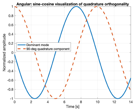
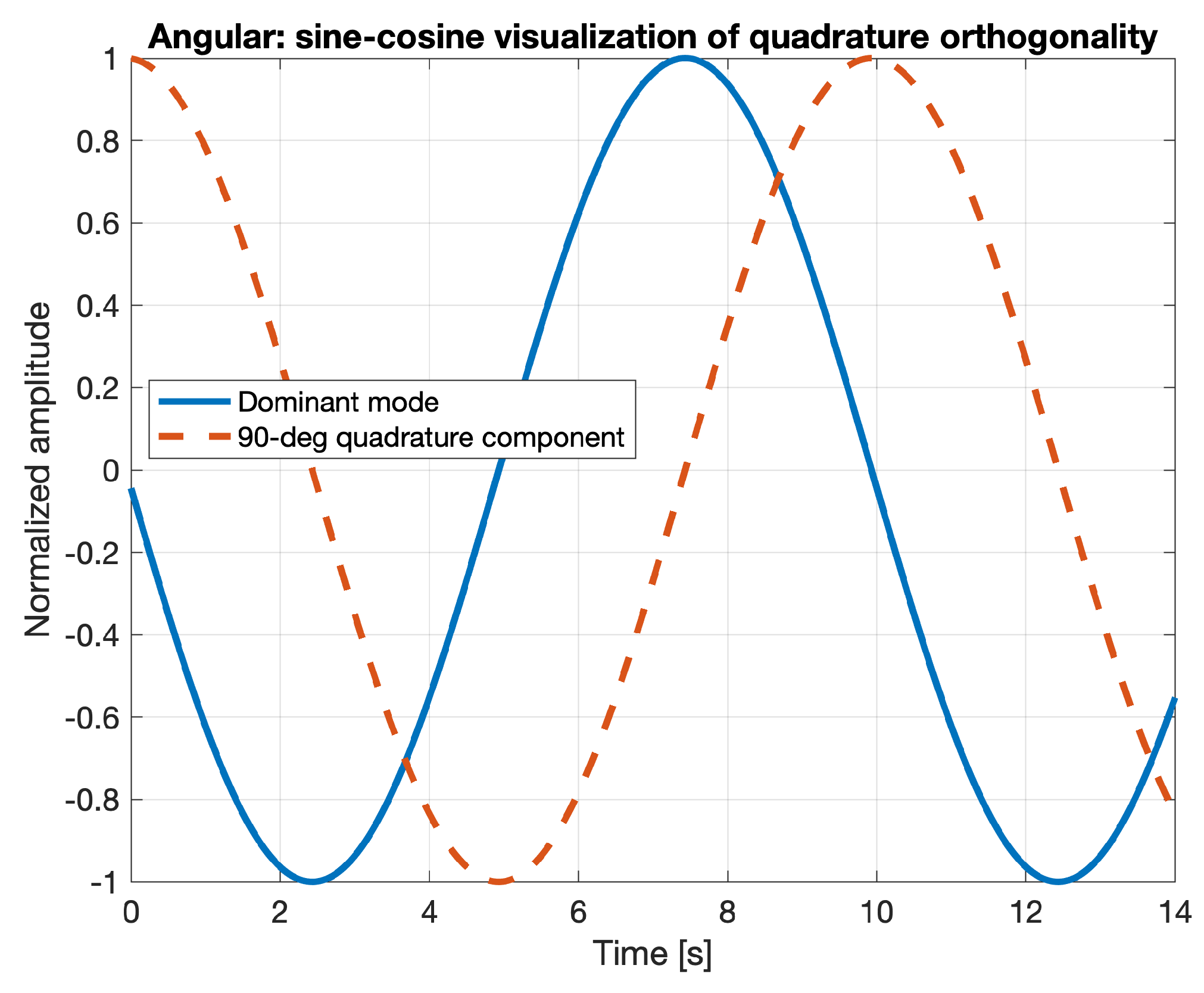
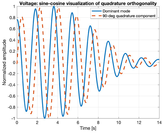
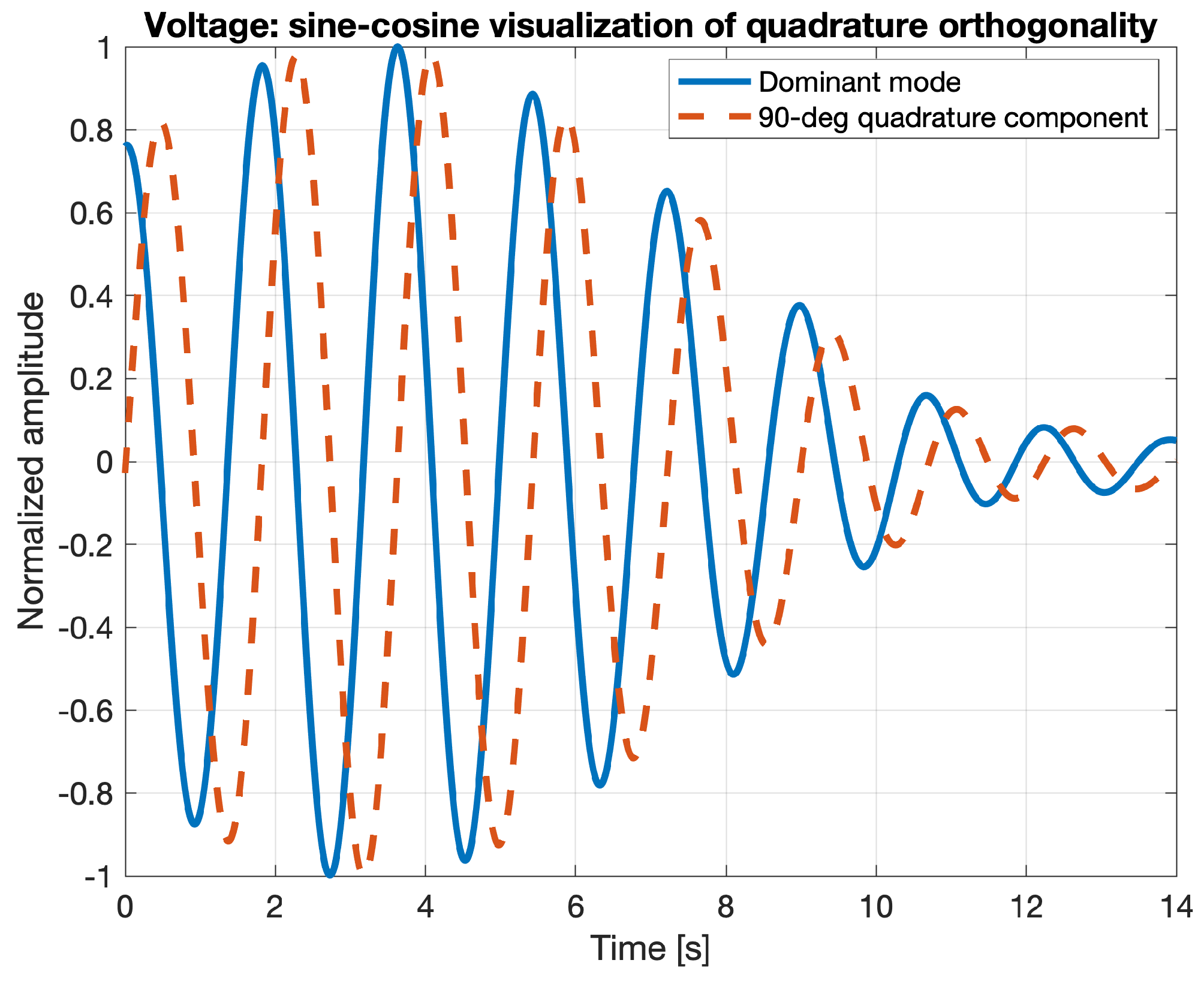
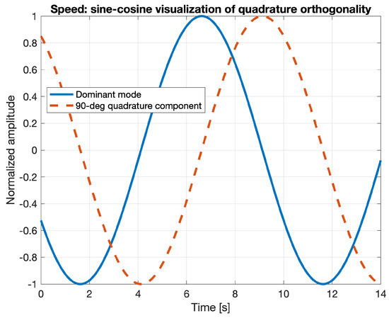
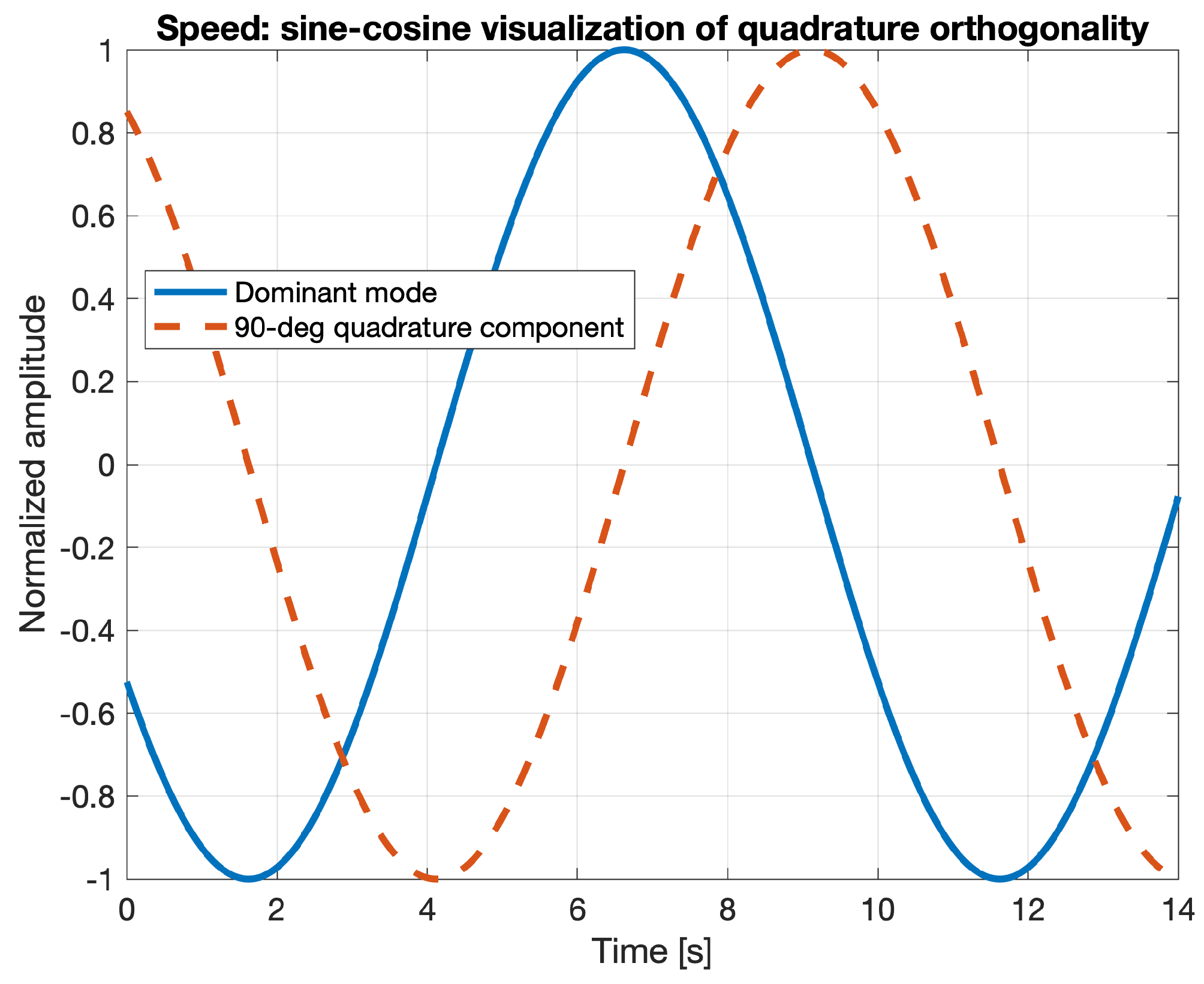
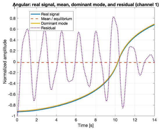
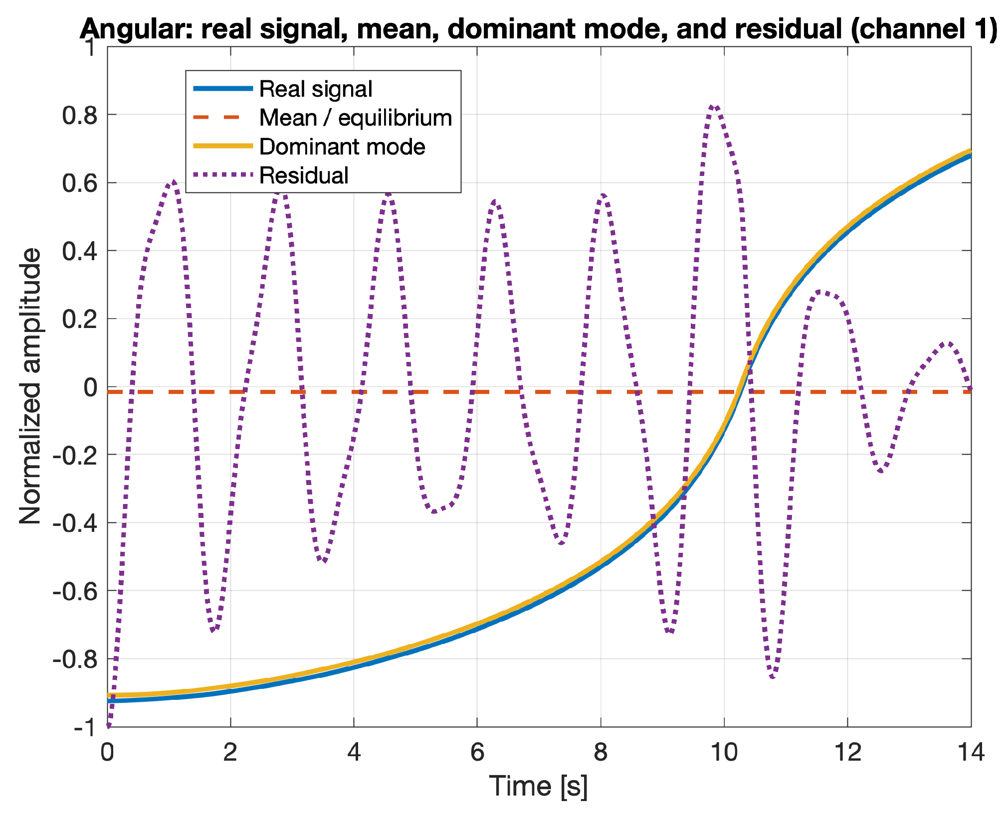
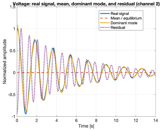
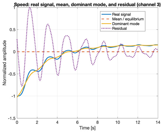
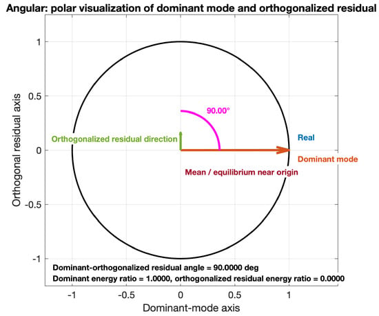
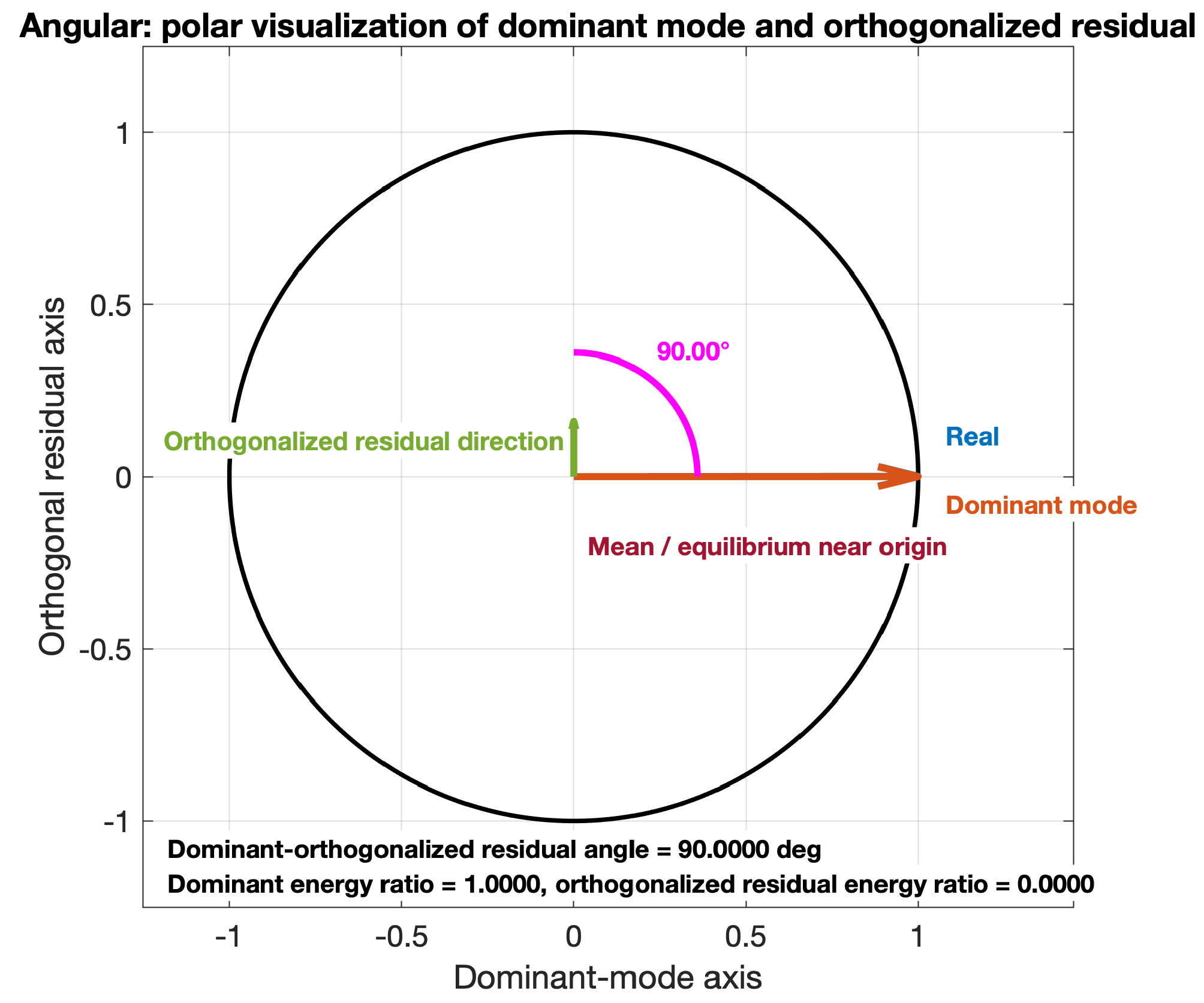
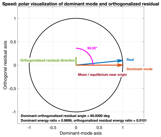
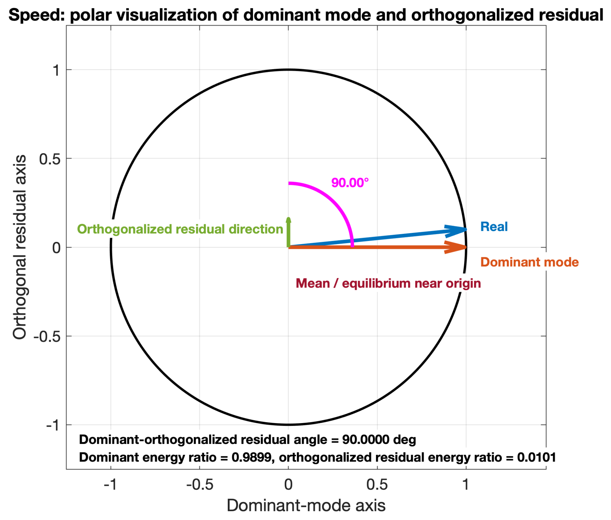
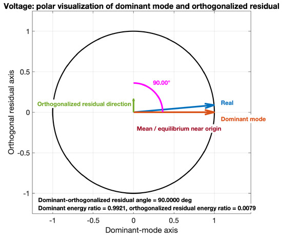
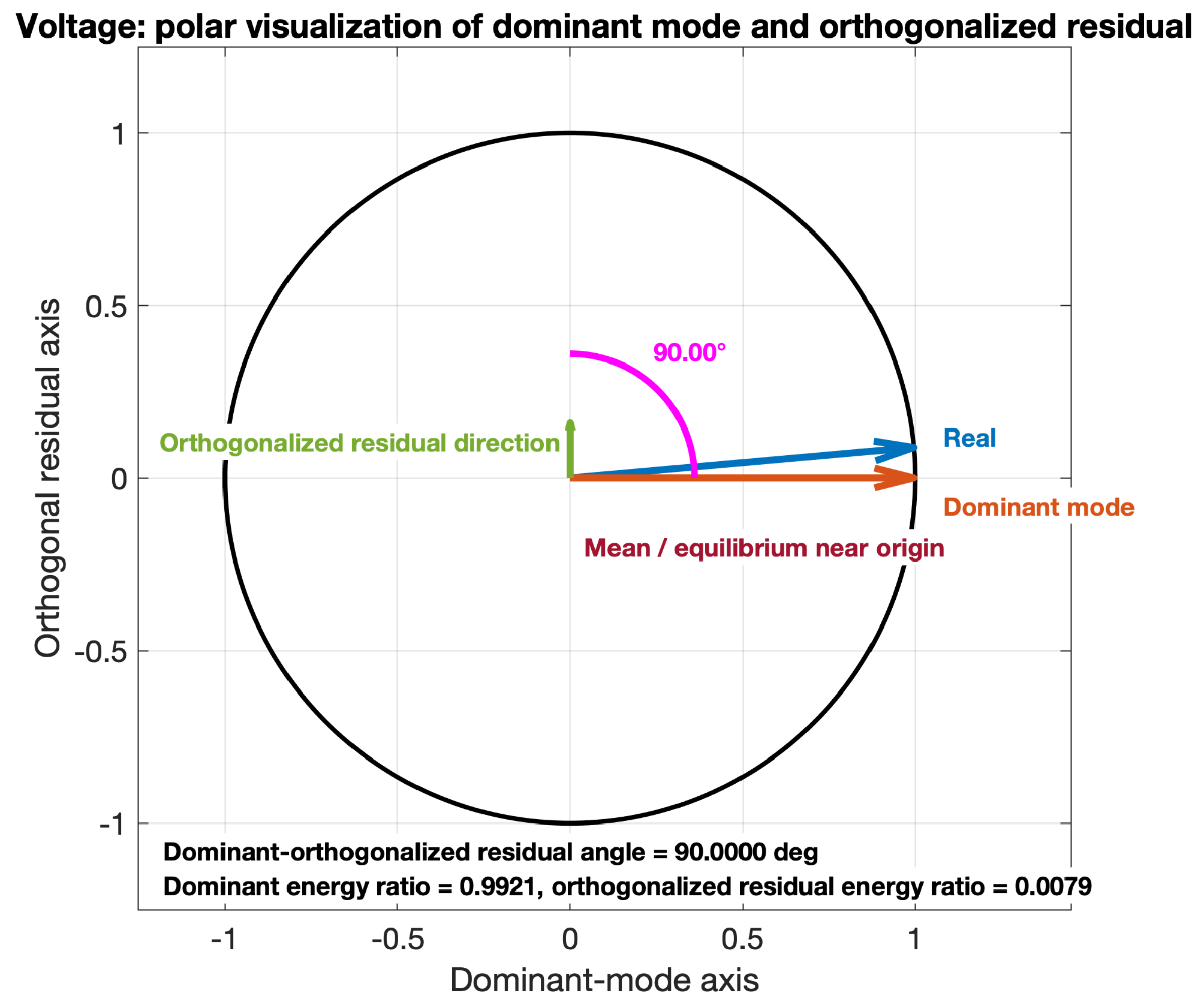

Disclaimer/Publisher’s Note: The statements, opinions and data contained in all publications are solely those of the individual author(s) and contributor(s) and not of MDPI and/or the editor(s). MDPI and/or the editor(s) disclaim responsibility for any injury to people or property resulting from any ideas, methods, instructions or products referred to in the content. |
© 2026 by the authors. Licensee MDPI, Basel, Switzerland. This article is an open access article distributed under the terms and conditions of the Creative Commons Attribution (CC BY) license.