An Infinite Precision Implementation of Regular Periodic Infinite Continued Fractions

Abstract

We give a detailed description of the process that is used to obtain the regular periodic continued fraction that represents $\sqrt{D}$, where D is a non-square positive integer. We give a new combinatorial proof of Lagrange’s theorem, showing that this process eventually enters a loop. We provide an infinite precision implementation of this process with the GMP library. We consider two algorithms for identifying the initial states, before the process reaches a state in the loop, and both require storing a constant amount of integers. Our experimental results show that the algorithm based on Galois’s criteria is faster than using Floyd’s algorithm, especially when the number of initial states is small. We also give an implementation of the inverse process of determining a degree-two polynomial that yields a particular continued fraction.

1. Introduction

We discuss a process for obtaining continued fractions that represent square roots, i.e., numbers of the form $\sqrt{D}$ where $D>1$ is a positive non-square integer. For example, $\sqrt{61}$ can be represented by an infinite periodic regular continued fraction as $7+1/(1+1/(4+1/(3+1/(1+1/(2+1/(2+1/(1+1/(3+1/(4+1/(1+1/(14+\dots )\left)\right)\left)\right)\left)\right)\left)\right)\left)\right)$, where the ellipsis portion can be replaced by the same expression without the initial 7. We use the following notation to represent this continued fraction is $[7;(1,4,3,1,2,2,1,3,4,1,14\left)\right]$. In this notation the periodic part of the fraction is shown inside parenthesis. The coefficients are separated by commas, except for the initial integer part, which uses a semicolon. For the fraction to be classified as regular, all the values should be positive integers, but the notation itself can be used with any number, so for example, $[0;0.5]=2$. The numerical representation of $\sqrt{61}$ is around $7.8102497$. Where the initial value of 7 is the integer part of $\sqrt{61}$. To obtain the next value in the expansion, we need to find the value y such that $\sqrt{61}=7+1/y$. Using some algebra this number simplifies to $y=(7+\sqrt{61})/12$. Now the integer part of this number is 1. This value is simpler to calculate as $\lfloor (7+7)/12\rfloor$. Hence we can again find the next number as ${(-1+(7+\sqrt{61})/12)}^{-1}$. This simplifies to $(5+\sqrt{61})/3$. Again, we can repeat this process by observing that the integer part of this number is $4=12/3$ and then obtain $(7+\sqrt{61})/4$. So far, this sequence of numbers has no indication of repeating but let us consider the full sequence:

$$\begin{array}{ccccccccccccc}x=\hfill & \hfill {\displaystyle \frac{0+\sqrt{61}}{1}}& \hfill {\displaystyle \frac{7+\sqrt{61}}{12}}& \hfill {\displaystyle \frac{5+\sqrt{61}}{3}}& \hfill {\displaystyle \frac{7+\sqrt{61}}{4}}& \hfill {\displaystyle \frac{5+\sqrt{61}}{9}}& \hfill {\displaystyle \frac{4+\sqrt{61}}{5}}& \hfill {\displaystyle \frac{6+\sqrt{61}}{5}}& \hfill {\displaystyle \frac{4+\sqrt{61}}{9}}& \hfill {\displaystyle \frac{5+\sqrt{61}}{4}}& \hfill {\displaystyle \frac{7+\sqrt{61}}{3}}& \hfill {\displaystyle \frac{5+\sqrt{61}}{12}}& \hfill {\displaystyle \frac{7+\sqrt{61}}{1}}\\ \lfloor x\rfloor =\hfill & \hfill 7& \hfill 1& \hfill 4& \hfill 3& \hfill 1& \hfill 2& \hfill 2& \hfill 1& \hfill 3& \hfill 4& \hfill 1& \hfill 14\end{array}$$

Now consider the last element in the sequence $7+\sqrt{61}$. Notice that its integer part is 14, by applying the usual transformation we obtain $(7+\sqrt{61})/12$. This number occurred as the second number in the sequence, thus this process will now repeat indefinitely.

In this paper we focus in achieving the following goals:

• Provide a detailed description of the process of computing the regular periodic infinite continued fraction of non-square integer D. We study this process both as a sequence of surds and as a sequence of degree-two polynomial roots, see Lemma 1. Except for Theorem 3, all other results apply to a general sequence of degree-two polynomials with real roots and integer coefficients that do not necessarily represent a square root of D.
• We give a new combinatorial proof that this sequence of numbers will eventually repeat, see Theorem 1. We also describe how to invert this process by obtaining a polynomial that produces a desired continued fraction, Theorem 2.
• We then describe how to implement these processes with the GNU MP library and how to use Floyd’s algorithm or Galois’s criteria to determine the size of the initial sequence and the size of the looping sequence in minimal space, Section 3.2. We experimentally validate the performance of our implementation, Section 4.

2. General Form

Let us consider the general procedure for generating these types of sequences. A general term in the sequence is represented by the variable x. Note that we always have $x>0$. We are only interested in the continued fraction representation of positive numbers of the form $\sqrt{D}$. We can observe that, in this example, the value D is constant throughout the process. This is true in general. The general form for x is then as follows:

$$x={\displaystyle \frac{-B+\sqrt{D}}{A}}$$

(1)

In this expression, A and B are integers. In the simple case when $B=0$ and $A=1$, the surd simplifies to the square root of D. Also note that this general form can be used to represent the square root of a rational number, i.e., $x=\sqrt{p/q}=\sqrt{pq}/q$. Hence we could use $A=q$, $B=0$, and $D=pq$. An interesting property of this expression is that the coefficient associated with $\sqrt{D}$ is always 1. It is not immediately clear why this should be so. We will explain why this property holds in a moment. Before that, let us summarized the information that is necessary to identify a state of the sequence. It consists of the integers A and B. The value of D is stored globally and not in the state information.

To explain why D remains invariant and that the coefficient of $\sqrt{D}$ is always 1, we need to consider an alternate form of representing x. For this goal we use a quadratic equation ${(Ax+B)}^2-D=0$. Now x is a zero of this equation. The  polynomial representation is useful in determining the transformation process. To start, we expand the polynomial into $A^2{x}^2+2ABx+B^2-D$. This representation has the desirable property that all the coefficients are integers. Moreover, we divide by $A\ne 0$ to have simple coefficients for the $x^2$ and x terms. Thus we will consider the following polynomial:

$$q\left(x\right)={\displaystyle \frac{{(Ax+B)}^2-D}{A}}=A{x}^2+2Bx+{\displaystyle \frac{B^2-D}{A}}$$

Again, x is a zero in this polynomial. Note that the surd in Equation (1) corresponds to the usual quadratic formula. In general, there are two solutions to a quadratic equation, which is normally represented by a ± sign. When $A>0$, the plus represents the largest solution and the minus the smallest one. We will always use a plus sign of for $\sqrt{D}$. Hence it is possible to represent the smallest solution by changing the sign of A and B. Hence the other zero of the quadratic equation is ${\displaystyle \frac{B+\sqrt{D}}{-A}}$. Incorporating these considerations into the expansion process means that, when A is positive, x is the largest zero of the quadratic equation $q\left(x\right)=0$ and, when A is negative, x is instead the smallest zero.

There is another question with the representation of $q\left(x\right)$. Is $(B^2-D)/A$ an integer? When this term is an integer, we say that Equation (1) is a canonical representation of the surd. In this case, it is possible to choose a degree-two polynomial $q\left(x\right)=A{x}^2+2Bx+C$ with integer coefficients. Moreover, by rewriting the formula for C, we obtain that $D=B^2-AC$. Therefore, the value of D is similar to the usual discriminate expression of the quadratic formula. In fact, it is the usual value divided by 4, i.e., $D=({\left(2B\right)}^2-4AC)/4$.

Even though not all representations are canonical, it is always possible to obtain a canonical form. To illustrate this point we consider the surd $(-1+\sqrt{5})/3$. Let us assume that a non-canonical has the following form:

$$x={\displaystyle \frac{-B^{*}+\sqrt{D^{*}}}{A^{*}}}$$

(2)

In this example, we have that $B^{*}=1$, $D^{*}=5$, and $A^{*}=3$. Now the expression $(B^{*2}-D^{*})/A^{*}$ evaluates to $-4/3$, which is not an integer. Note that this problem does not occur when the surd is a pure square root, i.e., when $B^{*}=0$ and $A^{*}=1$. In such a case $(B^{*2}-D^{*})/A^{*}=-D^{*}$, which is an integer. Hence transforming a non-canonical representation into a canonical representation is only necessary when computing the continued fraction representation of a generalized surd. In the remainder of this section we explain this process. Hence the reader who is only interested in the continued fraction representation of a square root can safely skip to Section 3.

We thus want to modify the surd representation, without  altering the actual value of x. Hence we multiply both the numerator and denominator by $|A^{*}|$. We thus obtain the following:

$$x={\displaystyle \frac{-B^{*}\left|A^{*}\right|+\sqrt{D^{*}{A}^{*2}}}{A^{*}\left|A^{*}\right|}}={\displaystyle \frac{-B+\sqrt{D}}{A}}$$

Hence, to obtain a canonical representation from a non-canonical one, we set $A=A^{*}\left|A^{*}\right|$, $B=B^{*}\left|A^{*}\right|$, and $D=D^{*}{A}^{*2}$. In our example, the resulting representation is $(-3+\sqrt{45})/9$, which represents the same value of x as before. In this representation $B=3$, $D=45$, and $A=9$. Hence the expression $(B^2-D)/A$ evaluates to $-36/9=-4$. This is indeed an integer, as 9 is a factor of $-36$.

It is straight forward to check that this procedure works in general as $A^{*}\left|A^{*}\right|$ will always be a factor of $B^{*2}{A}^{*2}-D^{*}{A}^{*2}$. Therefore, we can assume without loss of generality that the original representation was canonical and therefore $C=(B^2-D)/A=\mathrm{sgn}\left(A^{*}\right)(B^{*2}-D^{*})$ represents an integer. Note that, in this last expression, $\mathrm{sgn}\left(A^{*}\right)$ represents the sign of the value $A^{*}$. Again, for the above example, we obtain $C=+1\times (1-5)=-4$.

Also note that a canonical representation is not necessarily unique. We can further multiply both the numerator and denominator by some integer. For example, if we multiply the last configuration by 2, we obtain $(-6+\sqrt{180})/18$, which represents the same value of x as the previous forms. In general, we prefer the simpler canonical form, i.e., when the greatest common divisor of A, B, and C is 1. Still, this is not strictly necessary because the process we describe is still correct when A, B, and C have a non-trivial common factor. However, a GCD of 1 has the advantage of reducing the computational complexity of the underlying integer operations, addition, subtraction, multiplication, and division. For  completeness, note that, for $(-3+\sqrt{45})/9$, we have $A=9$, $B=-3$, and $C=-4$, with a GCD of 1, and for $(-6+\sqrt{180})/18$, we have $A=18$, $B=-6$, and $C=-8$ with a GCD of 2.

We will soon show that the value of D is invariant on the steps taken to compute the continued fraction, Section 3.1. This is not the case for the transformation from the non-canonical representation to the canonical one. In particular, in the example we considered, the initial value of $D^{*}$ was 5, but the value of D in the canonical representation was $45=9\times 5$, i.e., the value was multiplied by $A^2=9$. This is the case in general because the canonization process uses $D=D^{*}{A}^{*2}$.

3. Sequence Properties

In this section we describe the general computation procedure, along with several important properties. Section 3.1 contains a complete overview, but we delay proofs and details to Section 3.3.

3.1. Complete Overview

Now let us focus on a step of the process. We first determine the integer part of x as $p=\lfloor x\rfloor$. We then compute the next number y in the sequence using the following process:

$$\begin{array}{cc}\hfill y& =1/(x-p)={\left({\displaystyle \frac{-B+\sqrt{D}}{A}}-p\right)}^{-1}={\displaystyle \frac{-A}{(Ap+B)-\sqrt{D}}}={\displaystyle \frac{-A((Ap+B)+\sqrt{D})}{{(Ap+B)}^2-D}}={\displaystyle \frac{(Ap+B)+\sqrt{D}}{-q\left(p\right)}}\hfill \end{array}$$

Hence we can write y in the same form as x, i.e., $y=(-B^{\prime }+\sqrt{D})/A^{\prime }$. Given the above derivation, we obtain the following update formulas:

$$\begin{array}{cc}\hfill A^{\prime }& =-q\left(p\right)\hfill \end{array}$$

(3)

$$\begin{array}{cc}\hfill -B^{\prime }& =Ap+B\hfill \end{array}$$

(4)

This derivation established that the value of D is preserved, and so is the sign and coefficient of $\sqrt{D}$. Moreover, it also establishes that $A^{\prime }$ and $B^{\prime }$ are integers. From Equation (4) it is simple to conclude that $B^{\prime }$ is an integer because A, B, and p are also integers. Concluding that $A^{\prime }$ is an integer follows from Equation (3) and the fact that C is an integer, discussed in Section 2. Hence, to preserve this property, by induction, for all the elements in the sequence, we need an update formula for $C^{\prime }$. This can be obtained by studying the update process with the polynomial $q\left(x\right)$. We deduce the same update formulas if we transform the polynomial $q\left(x\right)$ into the polynomial $q^{\prime }\left(y\right)=A^{\prime }{y}^2+B^{\prime }y+C^{\prime }$ by applying the substitution $x=p+1/y$. We then multiply by $-y^2$ and collect similar terms:

$$q^{\prime }\left(y\right)=-(A{p}^2+2Bp+C)y^2-2(Ap+B)y-A=0$$

(5)

This yields the same update formulas as before and furthermore gives us the update $C^{\prime }=-A$. Hence we conclude that $C^{\prime }$ must also be an integer, given that A is known to be an integer.

Note that we can multiply the whole equation by $-1$. In this case the update formulas would become $A^{\prime }=q\left(p\right)$, $B^{\prime }=Ap+B$ and $C^{\prime }=A$. However, if we used these formulas, we would need also to keep track of the sign of $\sqrt{D}$. To avoid extra book-keeping we instead use the updates given by Equations (3) and (4).

In the surd representation it is clear that the value of D does not change in this process, i.e., $D^{\prime }=D$. However, in the polynomial representation, this fact is not immediate. It can be observed by evaluating $D^{\prime }=B^{\prime 2}-A^{\prime }{C}^{\prime }$ as follows:

$$D^{\prime }={(Ap+B)}^2-(A{p}^2+2Bp+C)A=B^2-AC=D$$

On the other hand, the polynomial update formulas are necessary to prove that, if the original coefficients are integers, the updated values are also integers, as explained. We can thus summarize the whole process in the following lemma:

Lemma 1.

Given a non-square positive integer D, it is possible to obtain its regular continued fraction representation $[p_1:p_2,\dots ]$ with values $p_i>0$ obtained as the integer part of a sequence of surds defined as $x_1=\sqrt{D}$ and $x_i=p_i+1/x_{i+1}$ with canonical representations as $x_i={\displaystyle \frac{-B_i+\sqrt{D}}{A_i}}>1$ and the following properties:

1. 

Values $A_i$, $B_i$, and $C_i=(B_i^2-D)/A_i$ are always integers.

2. 

$x_i$ is a solution of the quadratic equation $q_i\left(x\right)=A_i{x}^2+2B_{i}x+C_i=0$. If $A_i>0$, then $x_i$ is the largest solution; otherwise, $x_i$ is the smallest solution.

3. 

These values are updated as $A_{i+1}=-q_i\left(p_i\right)$, $-B_{i+1}=A_i{p}_i+B_i$, and $C_{i+1}=-A_i$.

We illustrate the values in this lemma, using the example with $D=61$.

$$\begin{array}{ccccccccccccccc}i\hfill & \hfill 1& \hfill 2& \hfill 3& \hfill 4& \hfill 5& \hfill 6& \hfill 7& \hfill 8& \hfill 9& \hfill 10& \hfill 11& \hfill 12& \hfill 13=2& \hfill \dots \\ \sqrt{61}\ge B_i=\hfill & \hfill 0& \hfill -7& \hfill -5& \hfill -7& \hfill -5& \hfill -4& \hfill -6& \hfill -4& \hfill -5& \hfill -7& \hfill -5& \hfill -7& \hfill -7& \\ A_i=\hfill & \hfill 1& \hfill 12& \hfill 3& \hfill 4& \hfill 9& \hfill 5& \hfill 5& \hfill 9& \hfill 4& \hfill 3& \hfill 12& \hfill 1& \hfill 12& \\ C_i=\hfill & \hfill -61& \hfill -1& \hfill -12& \hfill -3& \hfill -4& \hfill -9& \hfill -5& \hfill -5& \hfill -9& \hfill -4& \hfill -3& \hfill -12& \hfill -1& \\ p_i=\hfill & \hfill 7& \hfill 1& \hfill 4& \hfill 3& \hfill 1& \hfill 2& \hfill 2& \hfill 1& \hfill 3& \hfill 4& \hfill 1& \hfill 14& \hfill 1& \end{array}$$

This table contains the same information presented in the surd sequence, but arranged according to the notation of Lemma 1. Note that in this sequence the $A_i$ values are always positive and the $B_i$ values are always smaller than $\sqrt{61}$. The relation between these two observations is given by the following lemma.

Lemma 2.

During the execution of this process if $A_i>0$ then $B_i\le \sqrt{D}$; otherwise, if $A_i<0$, then $-\sqrt{D}\le B_i$.

The case where $A_i>0$ follows from Equation (1). For the other case, see the proof in Section 3.3. In essence, Lemma 2 restricts the range of values that $B_i$ can assume. However, this range of values is still infinite. Thus, to establish a restriction that forces the sequence of surds to repeat, we will show that the values of $B_i$ are actually strongly attracted to the interval $[-\sqrt{D},+\sqrt{D}]$. This forces the sequence of $B_i$ values to assume values inside this interval an infinite number of times. Therefore, the $B_i$ values will eventually repeat because the values are necessarily integers and there is only a finite number of integers inside this interval. This is the core of our proof.

Lemma 3.

If  $|B_i|>\sqrt{D}$, then $|B_i\left|>\right|B_{i+1}|$, for any index $i\ge 1$.

This is shown by using the update formula and proving that $B_i^2>B_{i+1}^2$, see Section 3.3. An interesting consequence of this lemma when combined with the formula $C_i=(B_i^2-D)/A_i$ from Lemma 1 is that, if for some value of i we have $C_i{A}_i>0$, then $C_i{A}_i>C_{i+1}{A}_{i+1}$. The lemma’s hypothesis may seem unlikely; in fact, it never occurs in the example table for $D=61$, near Lemma 1. However, it may indeed occur in a general sequence of surds. Another example table for $D=61$ is shown near Theorem 2, where the $|B_i|$ values form the sequence $\mathrm{245,725}>\mathrm{11,341}>336>\sqrt{D}=\sqrt{61}\approx 7.8102497$.

We can now complete our argument to show that the sequence of surds will eventually repeat.

Theorem 1

(Lagrange). For any non-square positive integer D, the value $\sqrt{D}$ can be represented by an infinite periodic regular continued fraction. More precisely, for the sequence of quadratic polynomials defined in Lemma 1, there exists an index $m\ge 0$ and a period of size n such that, for any index $i>m$, we have $q_i\left(x\right)=q_{i+n}\left(x\right)$.

Our argument uses the pigeon hole principle by noticing that the number of integers in the interval $[-\sqrt{D},\sqrt{D}]$ is finite and that Lemma 3 forces $B_i$ to return to this interval an infinite number of times. Likewise, we show that the corresponding $A_i$ is also forced to be chosen from a finite set. For the detailed proof, see Section 3.3.

There are several natural questions that can arise from these results. How large are the cycles in relation to D? What are the properties of $A_i$, $B_i$ when they are inside a cycle versus when they are in the initial phase? We will answer these questions shortly, as they provide further insight into the cycling process.

Our proof of Theorem 1 implies that, for both $A_i$ and $B_i$, values inside the cycle are limited to integers from a set of size $O\left(\sqrt{D}\right)$. Therefore, the maximum cycle will be $O\left(D\right)$. However, sharper bounds of $O\left(\sqrt{D}\log D\right)$ [1,2] are known.

By observing our current example we immediately notice that, for the values inside the cycle, the values of $A_i$ are always positive and therefore the values of $C_i$ are always negative. Moreover, inside the cycle we always observe $|B_i|\le \sqrt{D}$. These observations turn out to be true in general.

To establish these observations we also implemented the converse of the previous theorem, i.e., the process of determining D for a given cycle of n integers $p_{m+1},\dots ,p_{m+n}$. In fact, we implemented a function that, given a sequence of m numbers $p_1,\dots ,p_m$ and a cycle, outputs the values $A_1$, $B_1$, and D such that $x_1=[p_1;p_2,\dots ,p_m,(p_{m+1},\dots ,p_{m+n})]$ is a zero of the corresponding polynomial $q_1\left(x\right)$.

This is implemented in a two-step process. In the first step we determine $A_{m+1}$, $B_{m+1}$ and D for the corresponding cycle. In the second step we prepend the information related to the initial part of the fraction. To solve the first step we essentially need to write the equation $x_{m+1}=[p_{m+1};p_{m+2},\dots ,p_{m+n},x_{m+n+1}]$ and simultaneously have $x_{m+n+1}=x_{m+1}$. We can obtain a more explicit form for the right side of the equation by evaluating the convergents of the continued fraction. The i-th convergent is $h_i/k_i$, where $h_i$ and $k_i$ are positive integers. To maintain the indexes consistent throughout the presentation, we start the convergent sequence for $i=m+1$. Hence the integer sequence $h_i$ is defined, for $i>m$, recursively, as follows:

$$h_i=p_i{h}_{i-1}+h_{i-2}$$

(6)

Two base numbers need to defined, $h_m=1$ and $h_{m-1}=0$. The integers $k_i$ are defined with a similar recurrence to Equation (6). However, the base numbers are instead $k_m=0$ and $k_{m-1}=1$. Hence we can now write the desired equation for $x_{m+1}$.

$$x_{m+1}={\displaystyle \frac{x_{m+n+1}{h}_{m+n}+h_{m+n-1}}{x_{m+n+1}{k}_{m+n}+k_{m+n-1}}}$$

(7)

We can now simplify both $x_{m+1}$ and $x_{m+n+1}$ to $x=x_{m+1}=x_{m+n+1}$ and rearrange terms and multiply by two to obtain the following equation:

$$2k_{m+n}{x}^2+2(k_{m+n-1}-h_{m+n})x-2h_{m+n-1}=0$$

(8)

We have thus obtained the form of $q_{m+1}\left(x\right)$, where $A_{m+1}=2k_{m+n}$, $B_{m+1}=k_{m+n-1}-h_{m+n}$, and $C_{m+1}=-2h_{m+n-1}$. Moreover, the value of D can now be determined as $D={(k_{m+n-1}-h_{m+n})}^2+4k_{m+n}{h}_{m+n-1}$. Note that the $h_i$ and $k_i$ values are always non-negative integers, for any index i. The continued fraction representation of the root x that satisfies this equation is a purely periodic continued fraction.

In Lemma 4 we highlight some properties of the coefficients $A_i$, $B_i$, and $C_i$ inside the cycle. Note that it is possible to flip the signs of all the coefficient and still obtain the same roots. However, in our approach, we use a positive value of $A_{m+1}$ when considering the largest root of $q_{m+1}\left(x\right)$. Hence we need to verify that we are interested in the largest root of $q_{m+1}\left(x\right)$. For this, we observe that the formula for D implies that $B^2\le D$ and therefore that $\left|B\right|\le \sqrt{D}$, i.e., the hypothesis of Lemma 3 is false. This also implies that $-B-\sqrt{D}$ is necessarily a negative number, even when B is negative. Therefore, the smallest root of $q_{m+1}\left(x\right)$ is a negative number and not the desired root. We can now establish some properties for the coefficients inside the cycle.

Lemma 4.

Let m be the index described in Theorem 1. For any $i>m$, we have that $A_i>0$, $C_i<0$, $|B_i|<\sqrt{D}$, and $A_i+C_i>2B_i$.

This is a consequence of the formulation in Equation (8), see Section 3.3 for the proof.

It turns out that whenever the conditions $A_i>0$ and $C_i<0$ occur they are preserved by the update process and moreover also imply the other properties. Note that the next result does not require the restriction that i is inside the cycle.

Lemma 5.

For any quadratic polynomial $q_i\left(x\right)$ defined in Lemma 1, if $A_i>0$ and $C_i<0$, then $A_{i+1}>0$, $C_{i+1}<0$, $-\sqrt{D}<B_{i+1}<0$, and $A_{i+1}+C_{i+1}>2B_{i+1}$.

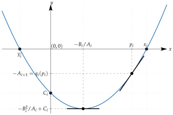
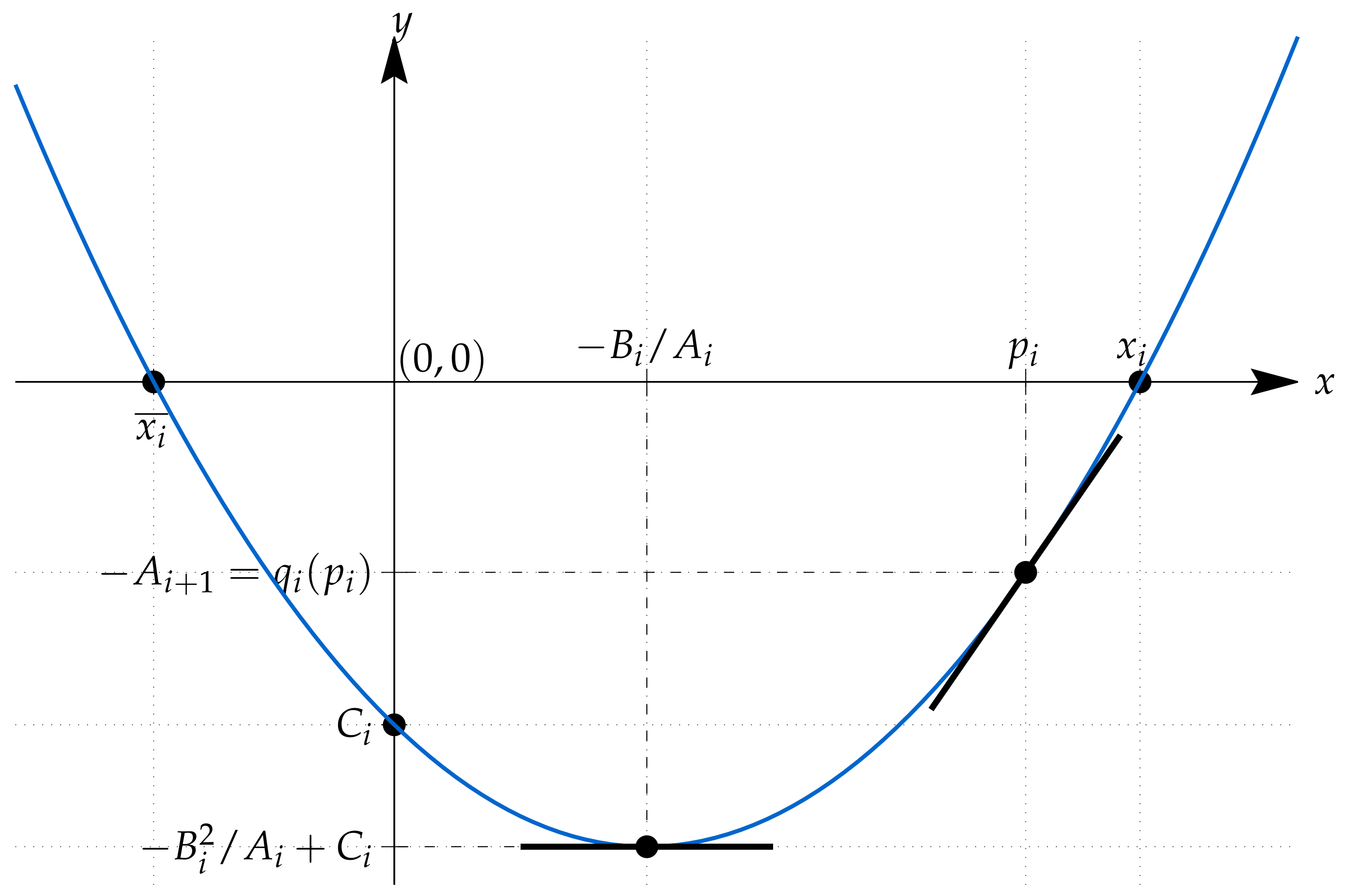
A schematic representation of the corresponding parabola is given in Figure 1, which illustrates the result. The formal proof is given in Section 3.3.

Figure 1. Plot of $q_i\left(x\right)$ in the conditions of Lemma 5.

This lemma provides insights into the proof of Theorem 1. Essentially, the lemma locks the sign configuration of the coefficients. Moreover, in this configuration, we have a solution for the Diophantine equation $B^2-AC=D$, where $-AC$ is a positive number. For a fixed value of D, there is a finite amount of such solutions. In fact, the size of these cycles is known to be bounded by $O\left(\sqrt{D}\log D\right)$ [1,2], although bounds based on the number of solutions to this Diophantine equation are a bit larger [3,4].

Before considering the second process, we highlight the mirror property, which will be relevant for Galois’s theorem. The previous process focused on determining the coefficients of the equation $x_{m+1}=[p_{m+1};p_{m+2},\dots ,p_{m+n},x_{m+1}]$. Let us simplify $x_{m+1}$ to x and write the equation more explicitly so that we can manipulate it. In essence, our goal is to transfer the p values from the right side of the equation to the left side. The following derivation gives an illustration of the process

$$\begin{array}{c}\hfill x=-(-x)=p_{m+1}+1/(p_{m+2}+1/(p_{m+3}+1/(\dots p_{m+n}+1/x\dots )))\\ \hfill -1/(p_{m+1}-x)=p_{m+2}+1/(p_{m+3}+1/(\dots p_{m+n}+1/x\dots ))\\ \hfill -1/(p_{m+3}+1/(p_{m+2}+1/(p_{m+1}-x)))=\dots p_{m+n}+1/x\dots \\ \hfill \dots \\ \hfill -1/(p_{m+n}+\dots 1/(p_{m+3}+1/(p_{m+2}+1/(p_{m+1}-x)))\dots )=1/x\\ \hfill 1/(p_{m+n}+\dots 1/(p_{m+3}+1/(p_{m+2}+1/(p_{m+1}-x)))\dots )=-1/x\\ \hfill \overline{1/(p_{m+n}+\dots 1/(p_{m+3}+1/(p_{m+2}+1/(p_{m+1}-x)))\dots )}=-1/\overline{x}\\ \hfill l1/(p_{m+n}+\dots 1/(p_{m+3}+1/(p_{m+2}+1/(p_{m+1}-\overline{x})))\dots )=-1/\overline{x}\\ \hfill 1/(p_{m+n}+\dots 1/(p_{m+3}+1/(p_{m+2}+1/(p_{m+1}+1/z)))\dots )=z\end{array}$$

Note that, in the last equation, we substituted $-1/\overline{x}$ by z and obtained a new equation. Note that, before the substitution, we apply the algebraic conjugate to both sides of the equation. This step is not strictly essential, but it makes the mapping from the roots of one equation to the roots of the other equation coincide with the variable substitution. In essence, the issue is that, if $x>0$, then $-1/x<0$ and therefore its continued fraction expansion cannot be obtained by using only positive integers $p_i$. Hence the expansion we obtain is actually the representation of $-1/\overline{x}>0$. Alternatively, the same derivation can be illustrated with continued fraction notation:

$$\begin{array}{c}\hfill x=-[-x]=[p_{m+1};p_{m+2},\dots ,p_{m+n},x]\\ \hfill -[0;-1/x]=[p_{m+1};p_{m+2},\dots ,p_{m+n},x]\\ \hfill -[p_{m+1};-1/x]=[0;p_{m+2},\dots ,p_{m+n},x]\\ \hfill -[0;p_{m+1},-1/x]=[p_{m+2};\dots ,p_{m+n},x]\\ \hfill -[p_{m+2};p_{m+1},-1/x]=[0;\dots ,p_{m+n},x]\\ \hfill -[0;p_{m+2};p_{m+1},-1/x]=[\dots ,p_{m+n},x]\\ \hfill \dots \\ \hfill -[0;\dots ,p_{m+2};p_{m+1},-1/x]=[p_{m+n};x]\\ \hfill -[p_{m+n};\dots ,p_{m+2};p_{m+1},-1/x]=[0;x]=1/x\\ \hfill p_{m+n};\dots ,p_{m+2};p_{m+1},-1/x] =-1/x\\ \hfill p_{m+n};\dots ,p_{m+2};p_{m+1},-1/\overline{x}] =-1/\overline{x}\\ \hfill p_{m+n};\dots ,p_{m+2};p_{m+1},z]=z\end{array}$$

The solution of the new equation on z is now such that its continued fraction expansion is the mirror of the original one. Stated in another way, $x=[p_{m+1};p_{m+2},\dots ,p_{m+n},x]$ and $z=[p_{m+n};\dots ,p_{m+2},p_{m+1},z]$. We can now consider this substitution from the point of view of the quadratic equation. In essence, we want to apply the substitution to the following equation:

$$A{x}^2+2Bx+C=0$$

Using the substitution $x=-1/\overline{z}$, we obtain the following:

$$\begin{array}{c}\hfill A/{\overline{z}}^2-2B/\overline{z}+C=0\\ \hfill -C{\overline{z}}^2+2B\overline{z}-A=0\\ \hfill \overline{-C{\overline{z}}^2+2B\overline{z}-A}=\overline{0}\\ \hfill -C{z}^2+2Bz-A=0\end{array}$$

To obtain the second form, we multiply both sides by $-z^2$. Note that we multiply by $-z^2$, instead of $z^2$, because we know that inside the cycle the value of C is negative and we want the coefficient of $z^2$ to be positive. Hence we conclude that, given a quadratic equation $q\left(x\right)=0$ such that its solution is a purely periodic continued fraction, it is possible to obtain a quadratic equation whose solution is the mirror continued fraction by flipping the sign of A and C and swapping them with each other. As an example of this lemma, consider the surd $(5+\sqrt{61})/3$, which we know is part of the cycle for $\sqrt{61}$. For this surd the corresponding equation is $9x^2-5\times 2x-4=0$ and the corresponding solution is $\left[\right(1;2,2,1,3,4,1,14,1,4,3\left)\right]$. Hence the corresponding equation on $z=-1/x$ is $4z^2-5\times 2z-9=0$ and the solution is the mirror $z=\left[\right(3;4,1,14,1,4,3,1,2,2,1\left)\right]$. In our example there is another equation that is worth pointing out in the context of this lemma. For the surd $(6+\sqrt{61})/5$ the corresponding equation is $5x^2-6\times 2x-5=0$. Notice that in this equation $A=-C$. Therefore, the lemma implies that the corresponding solution should be a mirror of itself. Hence the continued fraction expansion should be a palindrome. Indeed, we have that the solution is $x=\left[\right(2;1,3,4,1,14,1,4,3,1,2\left)\right]$.

Lemma 6.

If the largest solution of a quadratic equation $q\left(x\right)=A{x}^2+2Bx+C=0$, with integer coefficients, is a purely periodic continued fraction, then the largest solution of the quadratic equation $-C{z}^2+2Bz-A=0$ is the purely periodic continued fraction that mirrors x.

Let us now move on to the second process, prepending the initial sequence. For this we proceed backwards. We will determine $q_m\left(x\right)$ from $q_{m+1}\left(x\right)$. To use a notation similar to that of Equation (5), we write x for $x_m$, y for $x_{m+1}$, and $A^{\prime }$, $B^{\prime }$, and $C^{\prime }$ for the coefficients of $q^{\prime }\left(y\right)=q_{m+1}\left(y\right)$. Our goal is to now obtain the coefficients A, B, and C of $q\left(x\right)=q_m\left(x\right)$. Hence we rewrite the equation $x=p+1/y$, where $p=p_m$, to obtain $y=1/(x-p)$. We can now substitute this into $q^{\prime }\left(y\right)=0$. After some algebra we obtain the following equation:

$$-C^{\prime }{x}^2+2(C^{\prime }p-B^{\prime })x-(A^{\prime }-2B^{\prime }p+C^{\prime }{p}^2)=0$$

(9)

This therefore implies the following update formulas:

$$\begin{array}{cc}\hfill A& =-C^{\prime }\hfill \end{array}$$

(10)

$$\begin{array}{cc}\hfill B& =C^{\prime }p-B^{\prime }\hfill \end{array}$$

(11)

$$\begin{array}{cc}\hfill C& =-p^2{q}^{\prime }(-1/p)\hfill \end{array}$$

(12)

These formulas are chosen to perfectly invert the formulas of the forward direction. This can be seen by writing these processes in matrix form:

$$\left(\begin{array}{c}{A}^{\prime }\\ B^{\prime }\\ C^{\prime }\end{array}\right)=\left(\begin{array}{ccc}-p^2& -2p& -1\\ -p& -1& 0\\ -1& 0& 0\end{array}\right)\times \left(\begin{array}{c}A\\ B\\ C\end{array}\right)$$

(13)

$$\left(\begin{array}{c}A\\ B\\ C\end{array}\right)=\left(\begin{array}{ccc}0& 0& -1\\ 0& -1& p\\ -1& 2p& -p^2\end{array}\right)\times \left(\begin{array}{c}{A}^{\prime }\\ B^{\prime }\\ C^{\prime }\end{array}\right)$$

(14)

It can easily be checked that these two matrices are the inverse of each other. (It may be simpler to notice that, for $3\times 3$ triangular matrices of this type, the inversion formula is the following):

$${\left(\begin{array}{ccc}x& y& -1\\ z& -1& 0\\ -1& 0& 0\end{array}\right)}^{-1}=\left(\begin{array}{ccc}0& 0& -1\\ 0& -1& -z\\ -1& -y& -x-yz\end{array}\right)$$

Another interesting property of these matrices is that their determinate is $-1$. We could instead flip all the signs and have a determinate of 1, as this would not change the equations $q\left(x\right)=0$. However, we prefer this version as this way we obtain useful information from the sign of $A_i$, as explained in Lemma 1.

Besides the fact that these matrices are inverses, it is also necessary to show that $\lfloor x\rfloor =p$. This can be seen by substituting the update formulas into the surd form:

$$\begin{array}{cc}\hfill x& ={\displaystyle \frac{-B+\sqrt{D}}{A}}={\displaystyle \frac{-C^{\prime }p+B^{\prime }+\sqrt{D}}{-C^{\prime }}}=p+1/\left({\displaystyle \frac{-C^{\prime }}{B^{\prime }+\sqrt{D}}}\right)=p+1/\left({\displaystyle \frac{-C^{\prime }}{B^{\prime }+\sqrt{D}}}\right)\hfill \\ \hfill & =p+1/\left({\displaystyle \frac{-C^{\prime }(-B^{\prime }+\sqrt{D})}{D-B^{\prime 2}}}\right)=p+1/\left({\displaystyle \frac{-B^{\prime }+\sqrt{D}}{A^{\prime }}}\right)=p+1/y\hfill \end{array}$$

Hence, because we assumed $x_{i+1}=y>1$, it follows that p is indeed the integer part of x when using the previous backwards update formulas. Hence let us now summarize this process and move onto the discussion of how to implement it.

Theorem 2

(Euler). A number x with a continued fraction representation $[p_1;p_2,\dots ,p_m,(p_{m+1},$$\dots ,p_{m+n}\left)\right]$ can also be represented as a surd.

We can exemplify this prepending process by generating the equation $q\left(x\right)=0$ for $x=[4;5,6,7(1,\dots ,14\left)\right]$, given that we known that the equation for $x=[7;(1,\dots ,14\left)\right]$ is $1x^2+2\times 0x-61=0$. The resulting sequence of this process is the following:

$$\begin{array}{cccccccccc}i\hfill & \hfill 1& \hfill 2& \hfill 3& \hfill 4& \hfill 5& \hfill \dots & \hfill 15& \hfill 16=5& \hfill \dots \\ B_i=\hfill & \hfill -245,725& \hfill 11,341& \hfill -366& \hfill 0& \hfill -7& \hfill \dots & \hfill -7& \hfill -7& \\ A_i=\hfill & \hfill 58,596& \hfill -2195& \hfill 61& \hfill 1& \hfill 12& \hfill \dots & \hfill 1& \hfill 12& \\ C_i=\hfill & \hfill 1,030,459& \hfill -58,596& \hfill 2195& \hfill -61& \hfill -1& \hfill \dots & \hfill 12& \hfill -1& \\ p_i=\hfill & \hfill 4& \hfill 5& \hfill 6& \hfill 7& \hfill 1& \hfill \dots & \hfill 14& \hfill 1& \end{array}$$

This sequence is interesting as it illustrates cases where $A_i<0$ and $|B_i|>\sqrt{D}=\sqrt{61}$. As stated in Lemma 3, when this occurs, we should have $|B_i\left|>\right|B_{i+1}|$. We do in fact observe a decreasing sequence of these values $\mathrm{245,725}>\mathrm{11,341}>336>0$.

3.2. GNU MP Implementation

We will now discuss how to implement the process described in Lemma 1 and how to detect the cycle proven in Theorem 1. The first observation is how to compute $p_i$, the integer part of each surd $x_i$. We initially calculate the value $d=\lfloor \sqrt{D}\rfloor$ and use this integer throughout the process to determine $p_i$. If $A_i>0$, then we can use the following formula:

$$p_i=⌊{\displaystyle \frac{-B_i+\sqrt{D}}{A_i}}⌋=⌊{\displaystyle \frac{-B_i+\lfloor \sqrt{D}\rfloor }{A_i}}⌋=⌊{\displaystyle \frac{-B_i+d}{A_i}}⌋$$

(15)

Otherwise, if $A_i<0$, we instead have the following formula:

$$p_i=⌊{\displaystyle \frac{-B_i+\sqrt{D}}{A_i}}⌋=⌊{\displaystyle \frac{-B_i+⌈\sqrt{D}⌉}{A_i}}⌋=⌊{\displaystyle \frac{-B_i+1+d}{A_i}}⌋$$

(16)

We used the multiple-precision library GNU MP (https://gmplib.org/). To represent the information necessary to a given state, we use the struct quadratic, which stores the A and B values., see Listing 1.

Listing 1. Structure for storing A and B values.

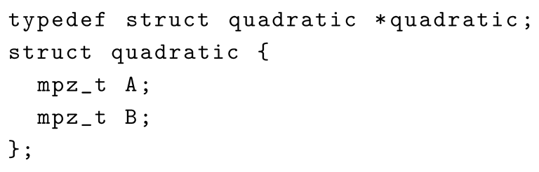The value of D is instead kept as a global variable. As explained the value of D is kept constant throughout the process. The value of C is also kept as a global variable this time because it can be obtained from A, B, and D.

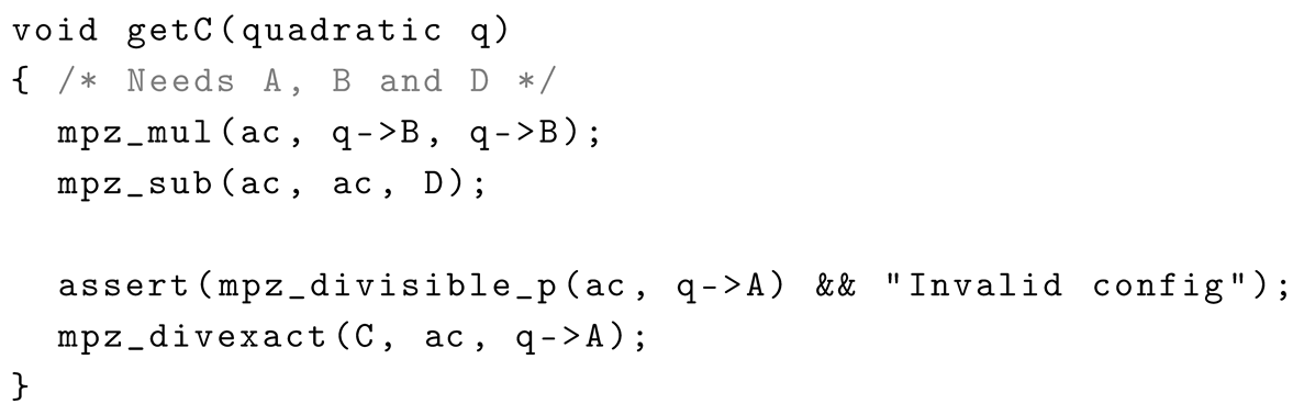
The function getC obtains the value of $C=(B^2-D)/A$, as stated in Lemma 1, omitting the index i, see Listing 2. We use the variable ac to hold intermediate calculations. The result is stored in the global variable C.

Listing 2. Implementation of getC.

The function floorx is used to determine the integer parts $p_i$ according to the formulas in Equations (15) and (16). The global variables d and $dp1$ store pre-computed values for $\lfloor \sqrt{D}\rfloor$ and $\lceil \sqrt{D}\rceil$, respectively, see Listing 3.

Listing 3. Implementation of floorx.

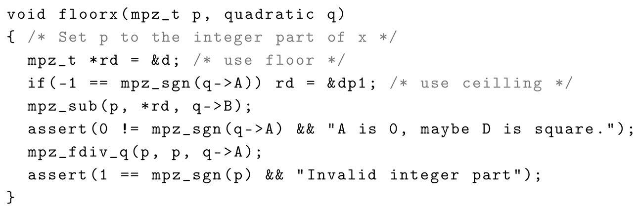The mpz_sgn function is used to check the sign of the corresponding integer. It returns $-1$, 0, or 1 when the sign is, respectively, negative, zero, or positive.

We now have the necessary components to implement the update process given in Equations (3) and (4). This is implemented in the function move, see Listing 4.

Listing 4. Implementation of move.

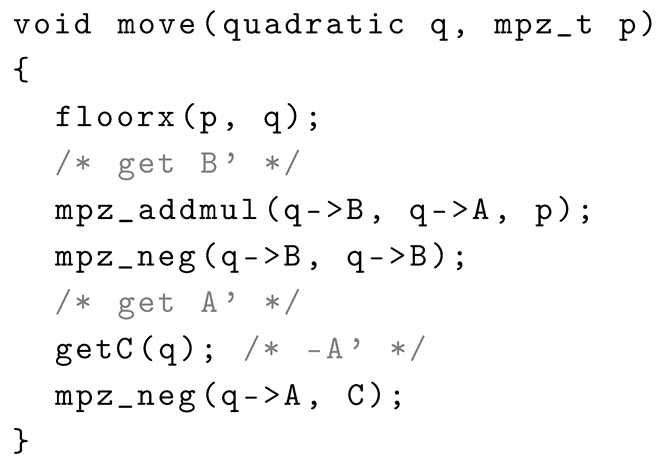In this implementation we use Equation (4) to update B to $B^{\prime }$. However, once this is carried out, we can no longer use Equation (3). Instead, we used the getC function, which gives $-A^{\prime }$ and then switches its sign.

It is fundamental to guarantee that the code executes correctly and does not output incorrect solutions or terminates unexpectedly. Towards this goal, we use the assert function to check that certain local properties hold. The argument of the function should always evaluate to true; otherwise, the function terminates the program to prevent incorrect outputs. In such cases it outputs the error message associated with the problem. In the context of this process, there are a couple of problematic cases that may occur. In the getC function, we need to check that A is a factor of $B^2-D$, before computing an integer division. In the floorx function we need to check that $A\ne 0$, before computing the surd division. Note that this can be the result of an incorrect input or the next step from a computation where D is a perfect square. In essence, when D is a perfect square, the first call to the move function will yield $A^{\prime }=0$. To see this, notice that in this case $D=d^2$ and the first integer part will be $p=(-B+d)/A$. Hence $q\left(p\right)$ evaluates to ${(Ap+B)}^2-D={(-B+d+B)}^2-d^2=0$. The last kind of error that we may encounter is the square root of a negative number, i.e., $D<0$. In fact, we need $D>0$, as $D=0$ is also problematic. The corresponding assert test is used in the discriminant function. (This function is omitted from the manuscript but is available in the git repository).

We consider two approaches to detect the cycle behavior. As a straightforward computational approach, we consider Floyd’s algorithm [5]. For this particular problem we can also consider a simple characterization of looping states, the Galois’s criteria.

First let us describe Floyd’s algorithm. The algorithm assumes that the discriminant function was computed, as this initializes the D, d, and dp1 global variables. Moreover, the Floyd function should not be called if the discriminant function reports any problem, see Listing 5. This may occur when D is a square or not positive. The algorithm keeps two states, h and t, also referred to as hare and turtle, respectively. The algorithms consists of two parts. In the first cycle both states use the move operation. However, the hare moves twice while the turtle one moves once. This difference in speed guarantees that the two states are always distinct while outside the cycle. Moreover, no matter the parity of the cycle size, the two states will eventually meet inside the cycle. At this point we found a state inside the cycle. Also, this state has some useful properties due to the process that was used to find it.

Listing 5. Implementation of Floyd’s algorithm.

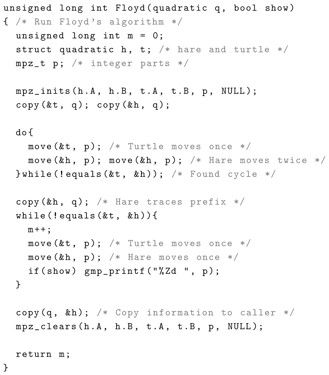Recall that the process starts at state $q_1$. We use the copy function to duplicate the information from the argument q into the turtle and hare structs. There are m steps until the first state inside the cycle is reached, i.e., state $q_{m+1}$. The size of the cycle is n, which means that $q_{m+1}=q_{m+1+n}$. In general, we have that $q_{m+j}=q_{m+j+kn}$, for any value $j\ge 1$ and $k\ge 0$. To check if the hare and the turtle are in the same state, we use the equals function, which returns true if both the hare and turtle struct quadratic store the same information.

Let w represent the number of states traversed by the turtle inside the cycle and s be the total number of steps performed by the turtle. Clearly, the number of steps performed by the hare is $2s$. Hence we have the following equations:

$$\begin{array}{cc}\hfill m+w& =s\hfill \end{array}$$

(17)

$$\begin{array}{cc}\hfill m+w+kn& =2s\hfill \end{array}$$

(18)

In these equations, k represents the number of times the hare loops around the cycle. Subtracting the first equation from the second one, we conclude that $kn=s=m+w$. Hence the size of the cycle is a factor of the number of steps taken by the turtle. Also, it gives us a way to subtract w from s to obtain m. This is performed in the second part of the algorithm. This time, the turtle and the hare move in sync. The hare re-starts at the beginning of the process, but the turtle continues from the state $q_{s+1}$. Hence, after m steps, the hare is at state $q_{m+1}$ and the turtle at state $q_{m+1+s}=q_{m+1+kn}=q_{m+1}$. Therefore, both the hare and the turtle meet in the first state of the cycle. Hence we can determine the value of m; this is the return of the Floyd function. Moreover, the identified state $q_{m+1}$ is copied to the argument structure and therefore passed back to the caller function. We can determine the same state with the Galois function. Once we determine the state $q_{m+1}$, we can simply move around the cycle to measure its size n. For this, we keep the turtle static and let the hare loop around the cycle. This is implemented by the Cycle function, see Listing 6.

Listing 6. Implementation of cycle.

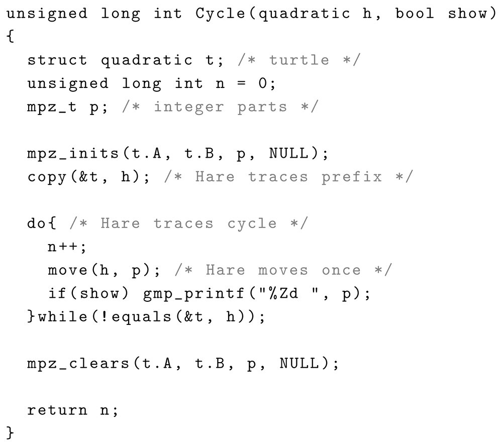Finally, note that all three of these functions receive an argument show that is used to printout the information related to the integer parts $p_i$ determined in the process. For example, for $q_1\left(x\right)=x^2-61$, we would obtain 7 (1 4 3 1 2 2 1 3 4 1 14).

To invoke Floyd’s algorithm, we instead use the letters F or D. In this case the input contains the coefficients A, B, and C or D depending on the given command. For example, both the following commands give the previous output.

• F 1 0 -61
  D 1 0 61

Likewise, to invoke the same result with Galois’s criteria, we use the letters G or H. So the previous output can also be obtained with the following lines:

• G 1 0 -61
  H 1 0 61

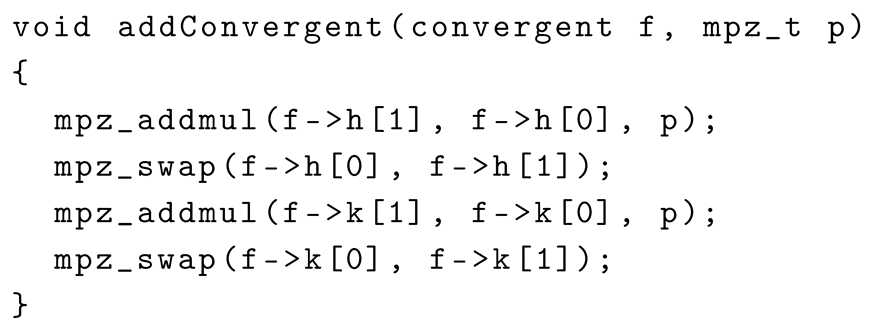
We also implemented the process described in Theorem 2. The addConvergent function updates the convergent information by applying Equation (6) to $h_i$ and $k_i$. The struct convergent stores a pair of values for h and a pair of values for k, see Listing 7.

Listing 7. Structure for storing hi and ki values.

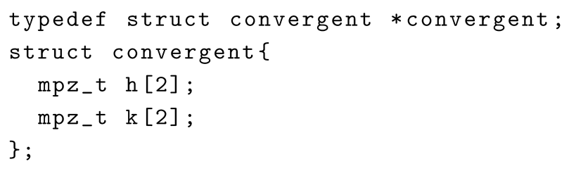We interpret the index 1 in the C array as the index $-1$ in our notation. Therefore, the value at index 0 is always the last computed value.

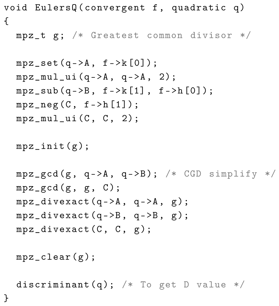
The addConvergent uses the mpz_addmul function to perform the desired computation, but the value is stored in the entry at index 1, see Listing 8. Therefore, it must be swapped to index 0 with the mpz_swap function. Once the convergents are computed, the coefficients $A_{m+1}$, $B_{m+1}$, and $C_{m+1}$ can be determined with Equation (8), see Listing 9. Our implementation simplifies A, B, and C so that their greatest common divisor is 1.

Listing 8. Implementation of addConvergent.

Listing 9. Coefficient computation according to Equation (8).

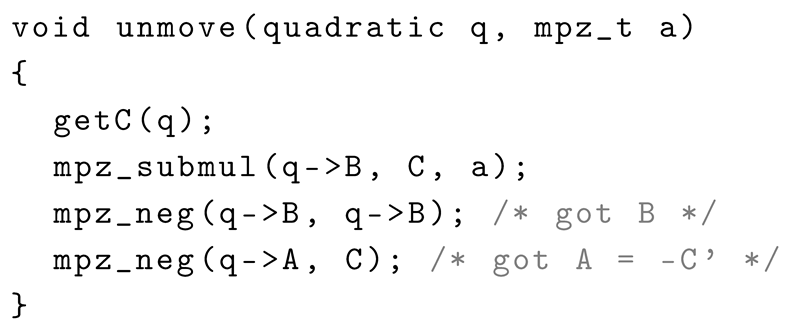
To implement the second part of Theorem 2, we use the function unmove, which implements the inverse of the move transformation, as described in Equation (14), see Listing 10.

Listing 10. Implementation of unmove.

For this second part, the numbers are given in reverse order. Hence, to obtain the example given before, we would input B 11 1 4 3 1 2 2 1 3 4 1 14 4 7 6 5 4.

The initial letter B indicates that we wish to build a polynomial. The number 11 is n. Next we input the 11 numbers that form the cycle $1,\dots ,14$. Then the number 4 represents m. Finally, the numbers we want to prepend before the cycle are given in reverse order since the computation is performed backwards as explained before. The resulting polynomial is outputted as 58,596 x^2 -245,725 * 2x +1,030,459.

We will now consider Galois’s criterion as a more efficient process for identifying the states inside the cycle.

Lemma 7

(Galois). For any quadratic polynomial $q_i\left(x\right)$ defined in Lemma 1, if $A_i>0$, $C_i<0$, and $A_i+C_i>2B_i$, then $x_i$ is part of the cycle, i.e., $i>m$ for the index m of Theorem 1.

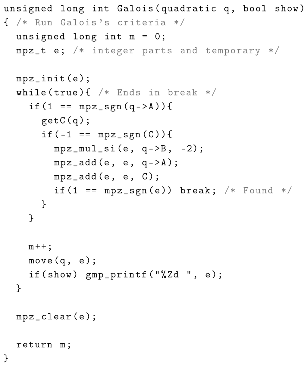
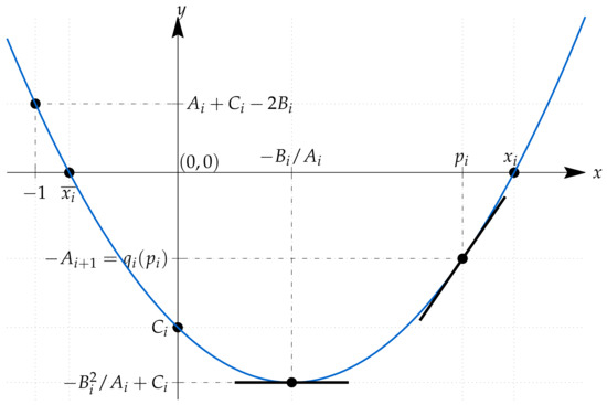
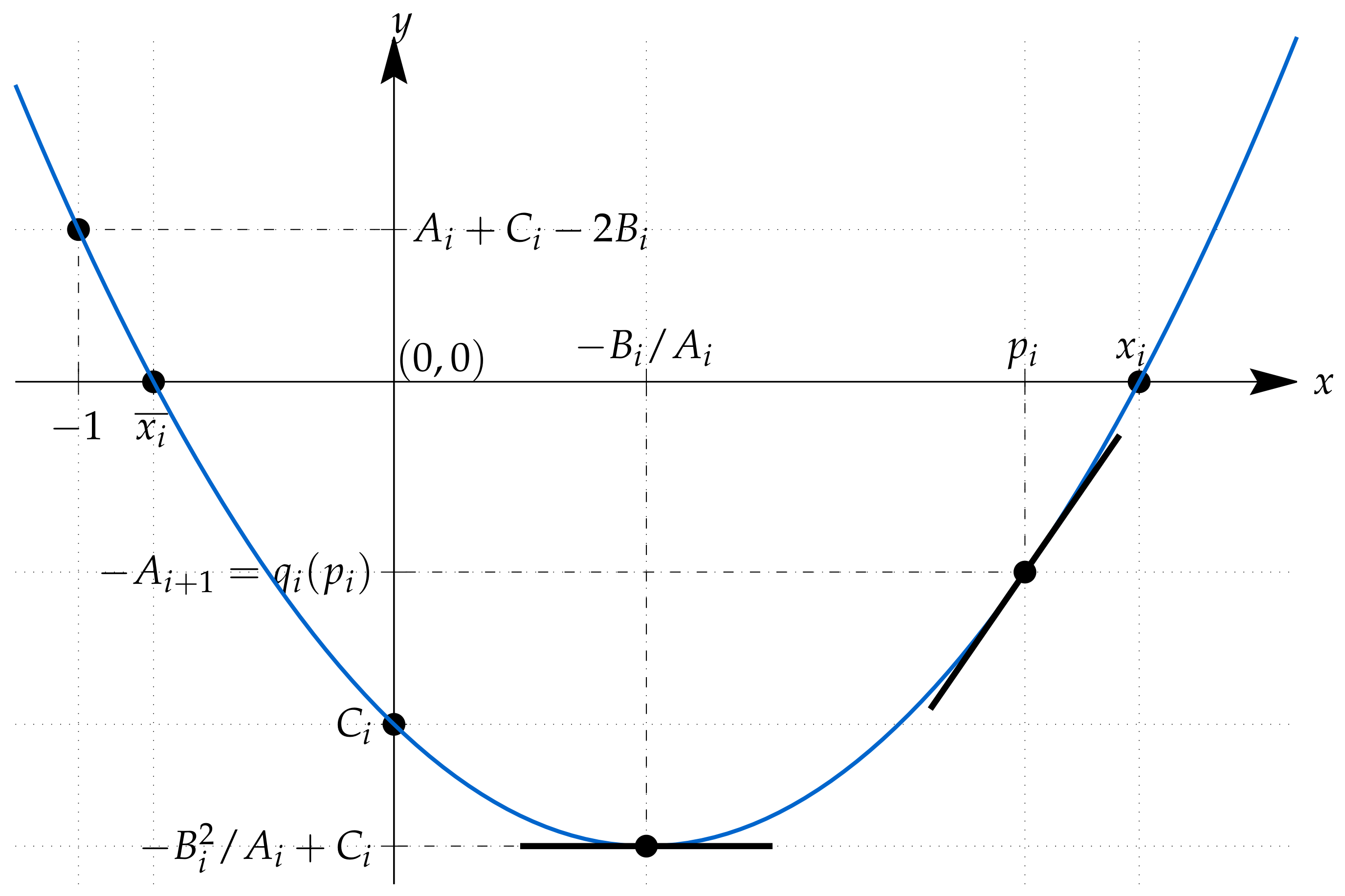
This gives a much simpler implementation of the cycle detection procedure, implemented in the function Galois, see Listing 11. A schematic representation of the corresponding parabola is Given in Figure 2. The formal proof focus on $\overline{x_i}$, the small root of the parabola. The proof is given in Section 3.3.

Figure 2. Plot of $q_i\left(x\right)$ in the conditions of Lemma 7.

Listing 11. Implementation of Galois’ criterion.

For completeness, we recall a fundamental consequence of Galois’s criteria. Let us consider the integer parts in the continued fraction expansion of $\sqrt{61}$. Note that, aside from the final value of $14=2\times 7=2\times \lfloor 61\rfloor$, the other coefficients inside the cycle form a palindrome, i.e., $p_1=p_{11}$, $p_2=p_{10}$, $p_3=p_9$, etc. This kind of structure occurs in general as described by the following theorem:

Theorem 3

(Galois). Given a non-square positive integer D, its regular continued fraction representation is of the form $[d:(p_2,\dots ,p_n,2d)]$, where $d=\lfloor \sqrt{D}\rfloor$, the size of the repeating values is n, and its initial part forms a palindrome, i.e., $p_{2+i}=p_{n-i}$ for any i between 0 and $n-2$.

This result is proven by using the update formulas with generic values d and $2d$, forward and backward, respectively, and applying Lemma 7. The proof is given in Section 3.3. The theorem states that the continued fraction representation of $\sqrt{D}$ contains an initial term of d that is not part of the periodic portion. The periodic portion starts at $p_2$, so according to our notation $m=1$. The $p_i$ values in the periodic part always form an even palindrome followed by the value $2d$. We can observe this structure in our example, where $\sqrt{D}=[7;(1,4,3,1,2,2,1,3,4,1,14)]$. In this case, $n=11$, the initial part of the periodic portion contains the even palindrome formed from $1,4,3,1,2$ and the value $14=2\times d$, because $d=7$. Likewise, $\sqrt{2}=[1;\left(2\right)]$, so $d=1$ and the palindromic part is empty. The palindromic part may also be an odd palindrome, as in the case of $\sqrt{3}=[1;(1,2)]$, where again $d=1$.

As a final command we also implemented a solution to Pell’s equation. This is a Diophantine equation of the form $x^2-D{y}^2=1$, where D is a given non-square integer, and x and y are the sought-out integer solutions of the equation. In these conditions, Lagrange proved that Pell’s equation has infinitely many distinct integer solutions. These solutions approximate $\sqrt{D}$ by rational numbers of the form $x/y$. These approximations can be obtained from the convergents of the continued fractions of $\sqrt{D}$. Our software outputs the fundamental solution, i.e., the one that minimizes x but is not the trivial solution $x=1$ and $y=0$. This can be obtained using the P command. Therefore, the input P 61 results in the following output:

• 1,766,319,049^2 - 61 * 226,153,980^2 = 1

Note that from the fundamental solution $x,y$, the remaining integer solutions $x_k,y_k$ can be obtained from the following equation, where k is a natural number:

$$x_k+y_k\sqrt{D}={(x+y\sqrt{D})}^k$$

(19)

Our implementation provides only the fundamental solution, which it obtains by computing the convergents of $\sqrt{D}$ and checking whether these values provide a solution to the equation.

3.3. Proofs

In this sub-section we give the proofs we omitted so far.

Proof of Lemma 1.

Most of the properties can be shown by induction. Clearly, in the base case, we have that $x_1>1$ can be represented as a surd, where $A_1=1$, $B_1=0$, and $C_1=-D$ are integers. The update formulas imply that $A_{i+1}$, $B_{i+1}$, and $C_{i+1}$ are also integers and that $x_{i+1}>0$, as discussed in the text.

We will now explain why the chosen update formula guarantees that there is no need to keep track of the signal of the $\sqrt{D}$ term, i.e., that when $A_i>0$ then $x_i$ is the largest zero of $q_i\left(x\right)$ and when $A_i<0$ then $x_i$ is the smallest zero of $q_i\left(x\right)$.

Let $x^{\prime }<x^{″}$ be the two zeros of $q_i\left(x\right)$. First assume that $A_i>0$, in which case $x_i=x^{″}$. In this case, we have $x^{\prime }-p_i<x^{″}-p_i$. We have two cases. If $\lfloor x^{\prime }\rfloor =p_i$, then $x^{\prime }-p_i>0$, in which case both terms are positive and we obtain that $1/(x^{\prime }-p_i)>1/(x^{″}-p_i)=x_{i+1}$. Hence $x_{i+1}$ is the smaller zero of $q_{i+i}\left(x\right)$ so $A_{i+1}=-q_i\left(p_i\right)$ should be negative, which is necessarily the case because $p_i<x^{\prime }$ and $-q_i\left(x\right)$ is a downwards-facing parabola. If $\lfloor x^{\prime }\rfloor <p_i$, then $x^{\prime }-p_i<0<x^{″}-p_i$, and therefore $1/(x^{\prime }-p_i)<1/(x^{″}-p_i)=x_{i+1}$. Hence $x_{i+1}$ is the larger zero of $q_{i+i}\left(x\right)$, so $A_{i+1}=-q_i\left(p_i\right)$ should be positive. Which is the case because $p_i$ is in between zeros of $q_i\left(x\right)$, i.e., $x^{\prime }<p_i<x^{″}$, and $-q_i\left(x\right)$ is a downwards-facing parabola.

Finally, we consider the case where $A_i<0$. In this case, $x_i=x^{\prime }<x^{″}$ and therefore $\lfloor x^{\prime }\rfloor =p_i$. Therefore, $x_i-p_i<x^{″}-p_i$. In this case, both terms are positive as $p_i<x^{\prime }<x^{″}$. Hence, by inverting the terms, the inequality changes, i.e., $x_{i+1}=1/(x_i-p_i)>1/(x^{″}-p_i)$. Hence $A_{i+1}=-q_i\left(p_i\right)$ should be positive, which is necessarily the case because $p_i<x^{\prime }$ and $-q_i\left(x\right)$ is an upwards-facing parabola.    □

Proof of Lemma 2.

For the first case we assume that $A_i>0$ and, by contradiction, that $B_i>\sqrt{D}$. Hence we conclude that $x_i=(-B_i+\sqrt{D})/A_i<0$, which contradicts the hypothesis of Lemma 1 that $x_i>1$.

For the second case we use a more elaborate deduction. Let us assume that $A_i<0$ and, by contradiction, that $B_i<-\sqrt{D}$. This implies that $B_i^2>D$ and therefore that $C_i=(B_i^2-D)/A_i<0$, because $A_i<0$. Hence we have all the values of $A_i$, $B_i$, and $C_i$ strictly smaller than zero, i.e., $A_i<0$, $B_i<0$, and $C_i<0$. Hence we get $A_i{x}^2<0$ and $2B_{i}x<0$ for any $x>0$. We can then add all these inequalities to obtain that $q\left(x\right)<0$ for any $x\ge 0$. Hence $q\left(x_i\right)=0$ must have $x_i<0$, which also contradicts the hypothesis of Lemma 1 that $x_i>1$.    □

Proof of Lemma 3.

To establish this property we consider the update formula of $B_i$. To  handle both cases of the sign of B, we square both sides and obtain the following:

$$B_{i+1}^2={(A_i{p}_i+B_i)}^2=A_i^2{p}_i^2+2A_i{B}_i{p}_i+B_i^2=A_i{p}_i(A_i{p}_i+2B_i)+B_i^2$$

Our goal is to show that $B_i^2-B_{i+1}^2>0$, which implies the desired result $|B_i\left|>\right|B_{i+1}|$. From the above derivation we conclude that $B_i^2-B_{i+1}^2=-A_i{p}_i(A_i{p}_i+2B_i)$. We now split the analysis into cases. When $A_i>0$, the first factor is smaller than zero, i.e., $-A_i{p}_i<0$. Moreover, from Lemma 2, we conclude that $B_i\le \sqrt{D}$. Recall that the hypothesis of Lemma 3 is that $|B_i|>\sqrt{D}$. Combining these two observations means that $B_i<-\sqrt{D}$. We can now show that $A_i{p}_i+2B_i<0$ with the following deduction:

$$\begin{array}{cc}\hfill A_i{p}_i+2B_i& <A_i\left({\displaystyle \frac{-B_i+\sqrt{D}}{A_i}}\right)+2B_i=-B_i+\sqrt{D}+2B_i=\sqrt{D}+B_i\hfill \\ \hfill & <\sqrt{D}-\sqrt{D}=0\hfill \end{array}$$

The other element of the deduction is the fact that $p_i$ is the largest integer that is smaller than the corresponding surd.

Now let us analyze the case when $A_i<0$. In this case, $-A_i{p}_i>0$. Hence we need to show that $A_i{p}_i+2B_i>0$. From the hypothesis of this lemma, we obtain that $B_i>\sqrt{D}>0$. We can combine this property with Lemma 2 and obtain the following deduction:

$$\begin{array}{cc}\hfill A_i{p}_i+2B_i& >A_i\left({\displaystyle \frac{-B_i+\sqrt{D}}{A_i}}\right)+2B_i=-B_i+\sqrt{D}+2B_i=\sqrt{D}+B_i>0\hfill \end{array}$$

Note that, for the first inequality, we have $p_i<(-B_i+\sqrt{D})/A_i$ combined with $A_i<0$.    □

Proof of Theorem 1.

Consider again the sequence of surds $x_i$ described in Lemma 1. It follows from Lemma 3 that the coefficients $B_i$ must be taken from the finite amount of integers in the interval $[-\sqrt{D},\sqrt{D}]$ an infinite amount of times. To  see this, notice that since all $B_i$ are integers, Lemma 3 actually implies that if $|B_i|>\sqrt{D}$ then $|B_i\left|-\right|B_{i+1}|\ge 1$. Hence iterating Lemma 3 means that if a given $B_i$ is outside this interval, it will become closer and closer to it until eventually, for some $i^{\prime }>i$, it will be such that $|B_{i^{\prime }}|\le \sqrt{D}$. Moreover, we can bound the value of index $i^{\prime }$ as $i^{\prime }-i\le \left|B_i\right|-\sqrt{D}$.

Now let us focus on the whole surd $x_i$, which depends on the values of $A_i$ and $B_i$. Thus far we have studied $B_i$ since $A_i$ is even simpler to pin to a finite set of integers. Note that, in Lemma 1, we have the formula $C_i=(B_i^2-D)/A_i$, where $C_i$ is necessarily an integer. This implies that $A_i$ is a factor of $B_i^2-D$. Hence, for a fixed value of $B_i$, there are only a finite amount of values that $A_i$ may assume. We thus conclude that the sequence of surds $x_i$ is such that the pairs of integers $(A_i,B_i)$ return a infinite amount of times to a finite amount of possibilities and therefore the sequence must eventually repeat one such pair. Let us assume that this repetition occurs at indexes $m+1$ and $m+n+1$, i.e., $(A_{m+1},B_{m+1})=(A_{m+n+1},B_{m+n+1})$. Now notice that the next state, $A_{m+2}$ and $B_{m+2}$, can be uniquely determined from $A_{m+1}$, $B_{m+1}$, and D, see Lemma 1. Recall also that D is invariant throughout the process. Hence we conclude that this implies that $(A_{m+2},B_{m+2})=(A_{m+n+2},B_{m+n+2})$. Likewise, the same argument can be repeated any number of times, and it therefore implies that the whole process repeats indefinitely.    □

Proof of Lemma 4.

As argued before, we have that $A_{m+1}=2k_{m+n}$. By induction we can show that this value is greater than 0. This follows from the calculation formula and the fact that the $p_i$ values are positive. Hence $A_{m+1}>0$. To conclude that these properties apply to all the coefficients $A_i$, $B_i$, and $C_i$ inside the cycle, and not just the very first one, note that the cycle can be rotated by swapping a suffix into a prefix. Our running example cycle is $(1,4,3,1,2,2,1,3,4,1,14)$, which can, for example, be rotated into $(3,4,1,14,1,4,3,1,2,2,1)$. Now the new quadratic polynomial $q_{m+1}^{\prime }$ is actually the original quadratic polynomial $q_{m+8}$. Thus this observation also applies to $A_{m+8}$ and in general to any of the quadratic polynomials inside the cycle. We can use the same argument for the sign of $C_i$, since $C_{m+1}=-2h_{m+n-1}<0$.

Finally, we now have that $A_i{C}_i<0$. Therefore, $B_i^2=D+A_i{C}_i$ implies $B_i^2<D$, which implies the desired property that $|B_i|<\sqrt{D}$.

Finally, note that the condition $A_i+C_i>2B_i$ reduces to checking that $2k_{m+n}-2h_{m+n-1}>2(k_{m+n-1}-h_{m+n})$. This is the same as checking that $k_{m+n}+h_{m+n}>k_{m+n-1}+h_{m+n-1}$, which is true as both the k and h values are strictly increasing.    □

Proof of Lemma 5.

The property that $C_{i+1}<0$ follows directly from the update formula $C_{i+1}=-A_i$ and the hypothesis $A_i>0$.

For the property $A_{i+1}>0$, we consider a schematic representation of $q_i\left(x\right)$ in the conditions of this lemma. We show such a scheme in Figure 1. The parabola faces upwards, because $A_i>0$. The  axis of the parabola is at x-coordinate $-B/A$. The parabola crosses the x-axis at two points and $x_i$ is the largest of the two. The integer $p_i$ is the floor of $x_i$. According to the update Formula (3), we have that $A_{i+1}=-q_i\left(p_i\right)$. Hence, to have $A_{i+1}>0$, we need to show that $p_i$ occurs in the part where the parabola is below the x-axis. For this, it is enough to show that $p_i$ cannot be smaller than the small root. We will instead show the stronger claim that $-B_i/A_i\le p_i$, as this is necessary to obtain the sign of $B_{i+1}$.

Assume by contradiction that $p_i\le -B_i/A_i$. We can then deduce that

$$\begin{array}{c}\hfill {\displaystyle \frac{-B_i+\sqrt{D}-A_i}{A_i}}=x_i-1<p_i\le -B_i/A_i\end{array}$$

From this, it follows that $D<A_i^2$. From Lemma 1 we have that $B_i^2-A_i{C}_i=D$, but the hypothesis of Lemma 5 implies that $-A_i{C}_i>0$ and therefore $B_i^2<A_i^2$. Therefore, we conclude that $-B_i/A_i<1$. Combined with the contradiction hypothesis, we conclude that $p_i<1$, which is absurd.

Therefore, we must have $-B_i/A_i<p_i$. This implies that $A_{i+1}>0$. It also implies that $B_{i+1}<0$. Recall the Formula (4), which is used to update the B coefficients. This formula is essentially $B_{i+1}=-q_i^{\prime }\left(p_i\right)/2$, where $q_i^{\prime }\left(x\right)$ represents the derivative of $q_i\left(x\right)$. Hence, to show that $B_{i+1}<0$, it is enough to show that the derivative of $q_i\left(x\right)$ is positive at $p_i$. This is true for all values larger than the axis, at $-B_i/A_i$. Therefore, the result follows from the inequality we have just shown, $-B_i/A_i<p_i$.

Recall that having $-A_{i+1}{C}_{i+1}>0$ implies that $B_{i+1}^2<D$ and therefore we get the desired bounds that $-\sqrt{D}<B_{i+1}<0$.

For the last property, we will verify that $A_{i+1}-2B_{i+1}+C_{i+1}>0$. According to the update Equation (13), we have the following derivation:

$$\begin{array}{cc}\hfill A_{i+1}-2B_{i+1}+C_{i+1}& =-A_i{p}_i^2-2B_i{p}_i-C+2A_i{p}_i+2B_i-A_i\hfill \\ \hfill & =-(A_i(p_i^2-2p_i+1)+2B_i(p_i-1)+C_i)\hfill \\ \hfill & =-q_i(p_i-1)\hfill \end{array}$$

Hence it is enough to show that $q_i(p_i-1)$ is negative. By  Lemma 1 we have that $1\le p_i$ and therefore $0\le p_i-1$. By looking at Figure 1, we can observe that $q_i\left(x\right)$ is negative for x in the interval $[0,p_i]$. Since $p_i-1$ is in this interval, the desired property is true.    □

Proof of Lemma 7.

Let us assume by contradiction that the statement is false. Consider the largest value of i for which the property fails, i.e., $q_i\left(x\right)$ is not part of the cycle but $q_{i+1}\left(x\right)$ is inside the cycle. Let p be the integer that is used to transition from $q\left(x\right)$ to $q^{\prime }\left(y\right)$, i.e., we have $x=p+1/y$. Because $q^{\prime }\left(y\right)$ is inside the cycle, there will be some other polynomial $q^{″}\left(z\right)$, which is also inside the cycle and that transitions to $q^{\prime }\left(y\right)$, letting r be the integer that is used for this transition. Hence we have that $z=r+1/y$. From these two conditions we conclude that $x-z=p-r$. Note that all the polynomials, $q\left(x\right)$, $q^{\prime }\left(y\right)$, and $q^{″}\left(z\right)$, follow the scheme in Figure 2. The  polynomial $q\left(x\right)$, by this hypothesis, and the polynomials $q^{\prime }\left(y\right)$ and $q^{″}\left(z\right)$, because of Lemma 4, as the states are inside the cycle. Hence x, y, and z are the largest roots of the corresponding equations.

Note that our hypothesis states that $A>0$, $q\left(0\right)=C<0$ and $q(-1)=A+C-2B>0$. Hence Bolzano’s theorem implies that there is a root of $q\left(x\right)$ in $]-1,0[$, see also Figure 1. This is not the root we are calculating, i.e., the largest root. Instead it is the smaller root, the one that contains the $-\sqrt{D}$ radical. We represent the smaller root as $\overline{x}$, where the bar represents an automorphism  on $\mathbb{Q}\left[\sqrt{D}\right]$, that preserves $\mathbb{Q}$ and consists of changing the sign of $\sqrt{D}$. For completeness, this notation represents the complex conjugate of x, and the fact that it is also a root of $q\left(x\right)$ follows from the complex conjugate root Theorem [6]. Using these properties we have that $\overline{x}-\overline{z}=\overline{x-z}=\overline{p-r}=\overline{p}-\overline{r}=p-r.$ Again, considering the scheme in Figure 2, we conclude that both $\overline{x}$ and $\overline{z}$ must lie in $[-1,0]$, in which case $|\overline{x}-\overline{z}|<1$. This implies that $|p-r|<1$ and therefore $p=r$, as both p and r are integers. Hence the polynomials $q\left(x\right)$ and $q^{″}\left(z\right)$ are the same and $q\left(x\right)$ is inside the cycle with yields a contradiction.    □

Proof of Theorem 3.

Recall that the first polynomial used for the expansion of $\sqrt{D}$ is $q_1\left(x\right)=x^2-D$. From this polynomial we obtain $q_2\left(x\right)=(D-d^2)x^2-2dx-1$, using the update described in Lemma 1. It is straightforward to check that $q_2\left(x\right)$ verifies Galois’s criteria, Lemma 7, as  $D-d^2>0$, $-1<0$ and $D-d^2-1\ge 0>-2d$. Hence $q_2\left(x\right)$ is already inside the cycle and thus only the value $p_1=d$ is outside the cycle. We can now use $q_2\left(x\right)$ to obtain $q_{n+1}\left(x\right)$ by moving backwards, i.e., using the update in Equations (10)–(12), with  $p=2d$. This yields $q_{n+1}\left(x\right)=1x^2+2(d-2d)x+d^2-D-4d^2+{\left(2d\right)}^2=x^2-2dx-(D-d^2)$. Hence we can observe that $q_2\left(x\right)$ and $q_{n+1}\left(x\right)$ are very similar; in fact, we can obtain one from the other by flipping the signs of the coefficients of $x^2$ and $x^0$ and swapping them with each other. This is the mirroring transformation we summarized in Lemma 6. Hence the sequence from $q_2\left(x\right)$ moving forward is the same as moving backwards from $q_{n+1}\left(x\right)$. Thus the resulting sequence forms a palindrome.    □

4. Experiments

Our implementation, including the scripts we used to perform the following experiments are publicly available at https://github.com/LuisRusso-INESC-ID/RegularPICF (accessed on 6 July 2026).

We setup a couple of experiments to test the performance of our implementation. We expect the approach based on Floyd’s algorithm to always require $O(n+m)$ steps both for determining n and m. However, Galois’s criteria require only $O\left(m\right)$ steps to determine m and $O(m+n)$ steps to determine n. Both algorithms need to store only a constant $O\left(1\right)$ amount of states. However, the actual amount of bits necessary will be $O(1+\log (\max A,B,C,D\left)\right)$. Moreover, computing operations over large integers is also not constant. Adding or subtracting two b bit numbers requires $O(b/W)$ time, where W is the size of the computer word. However, multiplication requires algorithms based on the FFT, see Schönhage and Strassen [7], and requires $O\left(\right(b/W\left)\log b\right)$ time. Hence each step of the algorithm actually has this complexity instead of constant time. Therefore, for $b=\lceil 1+\log \left(\max A,B,C,D\right)\rceil$, the overall time performance of the algorithms will be $O\left(\right(n+m\left)\right(b/W\left)\log b\right)$ time for Floyd’s algorithm and $O\left(m\right(b/W\left)\log b\right)$ time for Galois’s criteria to determine m. Moreover, if we consider the initial processing step to compute a canonical surd, which may include a call to the mpz_gcd function, the overall time becomes $O\left(\right(n+m+b\left)\right(b/W\left)\log b\right)$ and $O\left(\right(n+b\left)\right(b/W\left)\log b\right)$, respectively. The precise space bound of all these algorithms is just $O(b/W)$.

The tests were executed in a PC equipped with an Intel(R) Core(TM) i5-4278U CPU @ 2.60GHz and 7.6 GiB of RAM running Linux I 6.13.8-arch1-1. The algorithms are written in C and compiled with 14.2.1 20250207 with optimization flags -O9 and linked with the GMP version 6.3.0-2.

To measure the space and time resources we used the time command. It outputs both the “Elapsed real time (in seconds)” and the “Maximum resident set size of the process during its lifetime, in Kbytes.”. To guarantee time precision, the process is forced to run up to at least 5 s, repeating the calculation of the same input instance. The estimated time for each run was obtained by dividing the total time by the number of repetitions. The tests where executed with no background processes that might affect real-time performance.

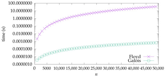
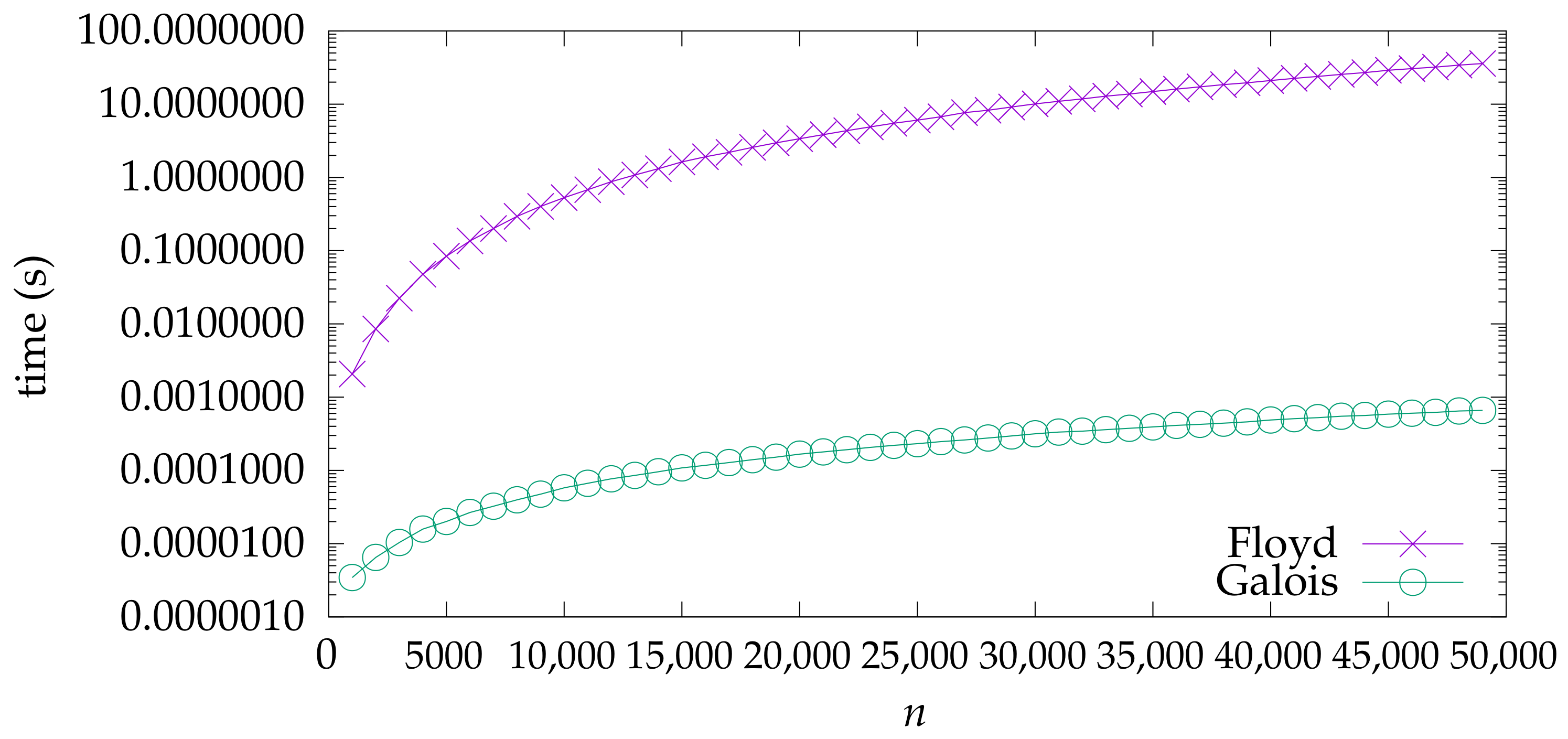
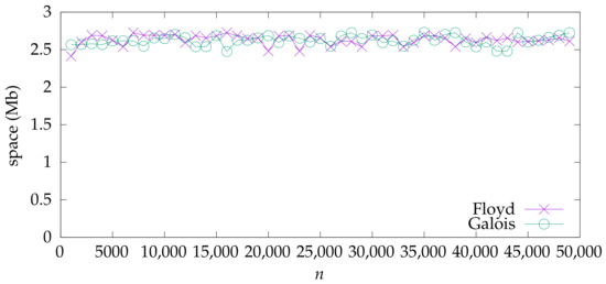
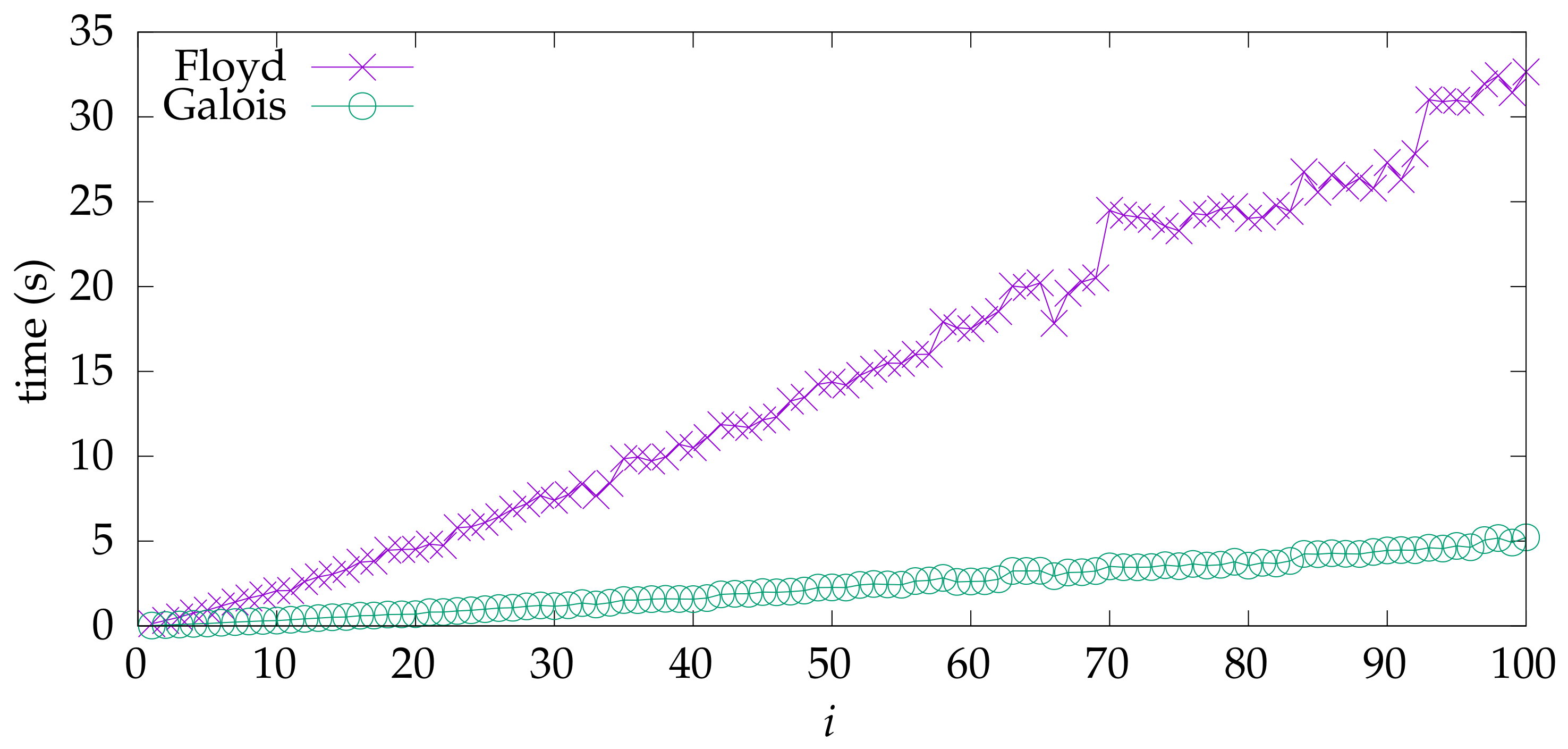
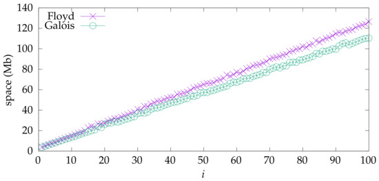
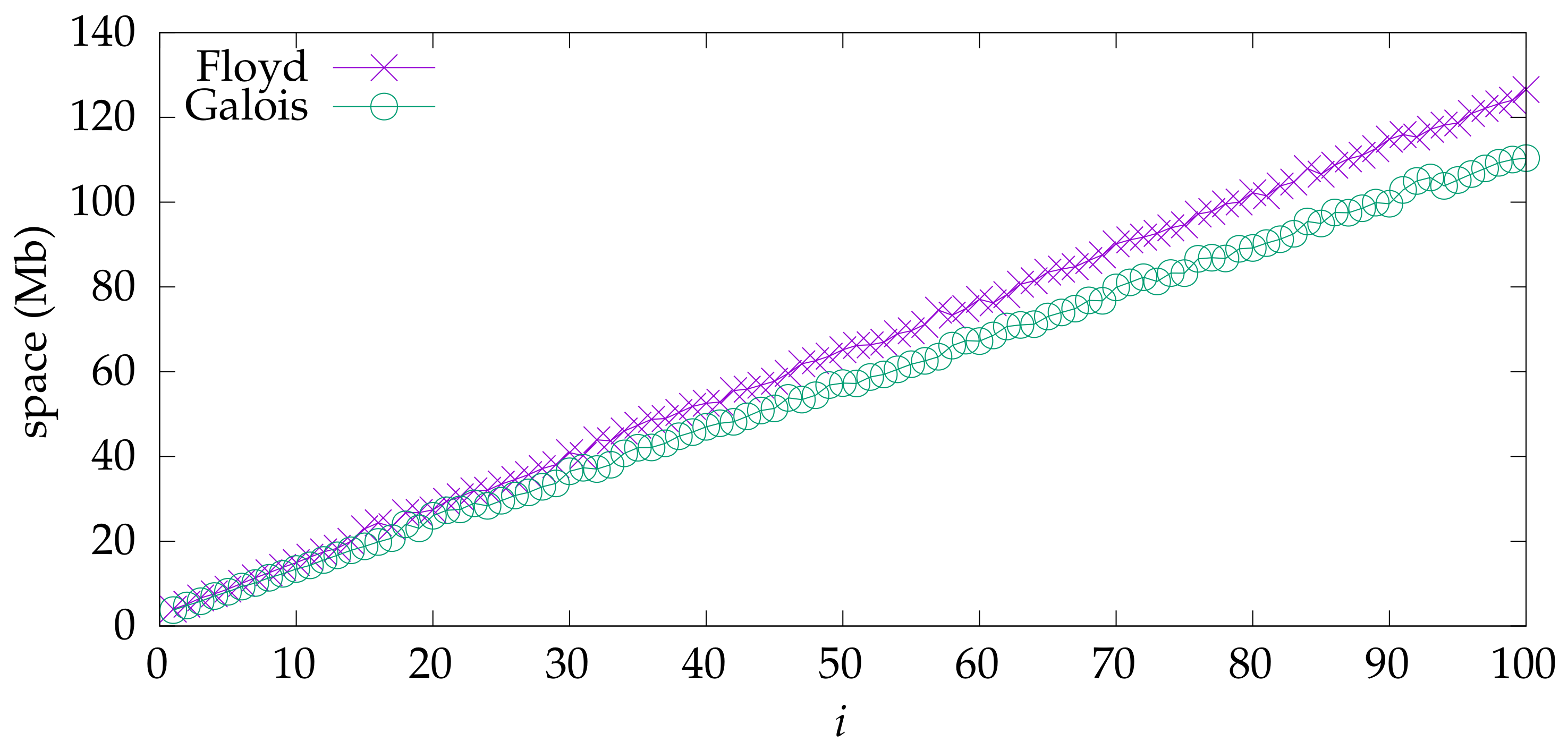
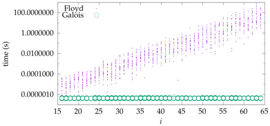
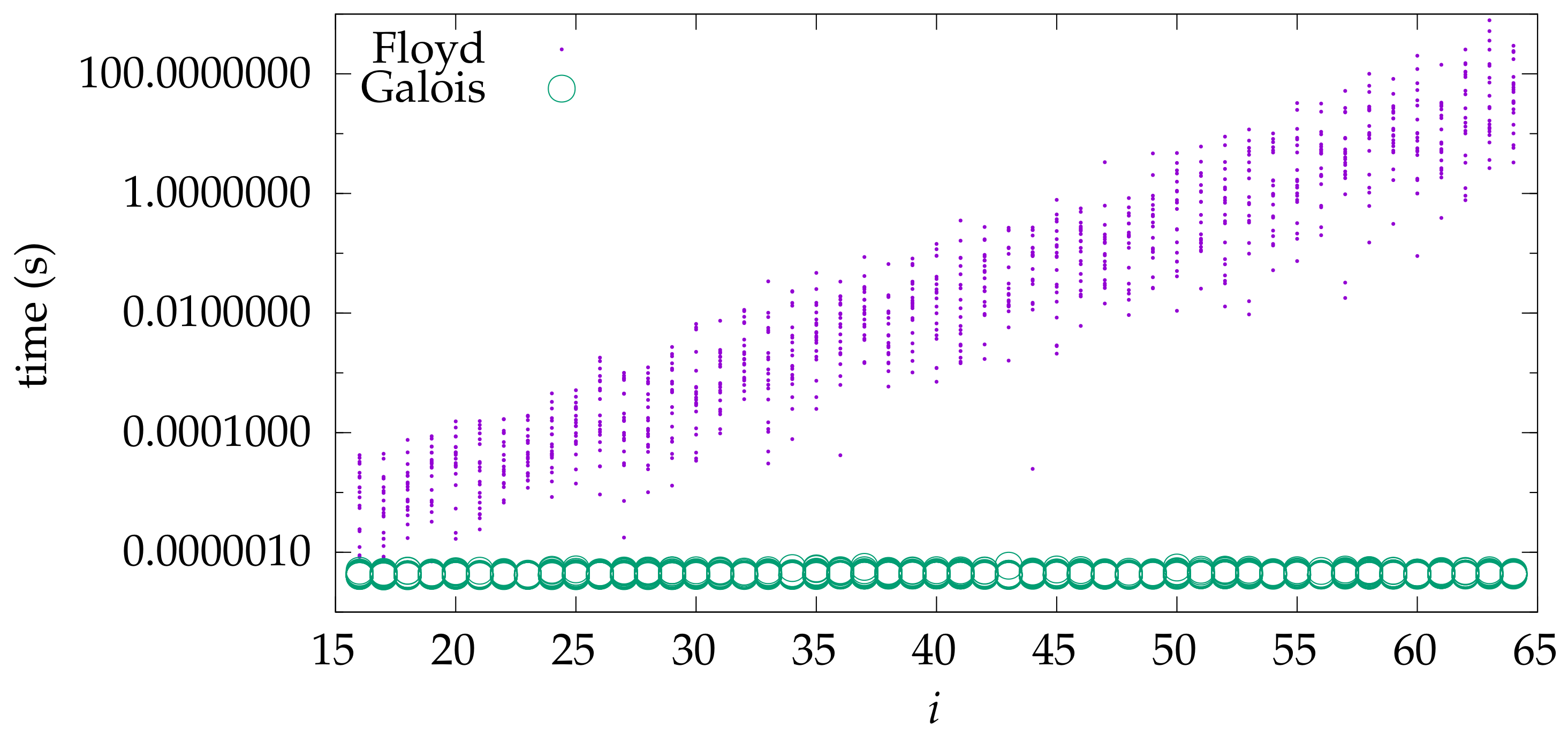
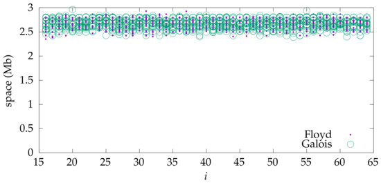
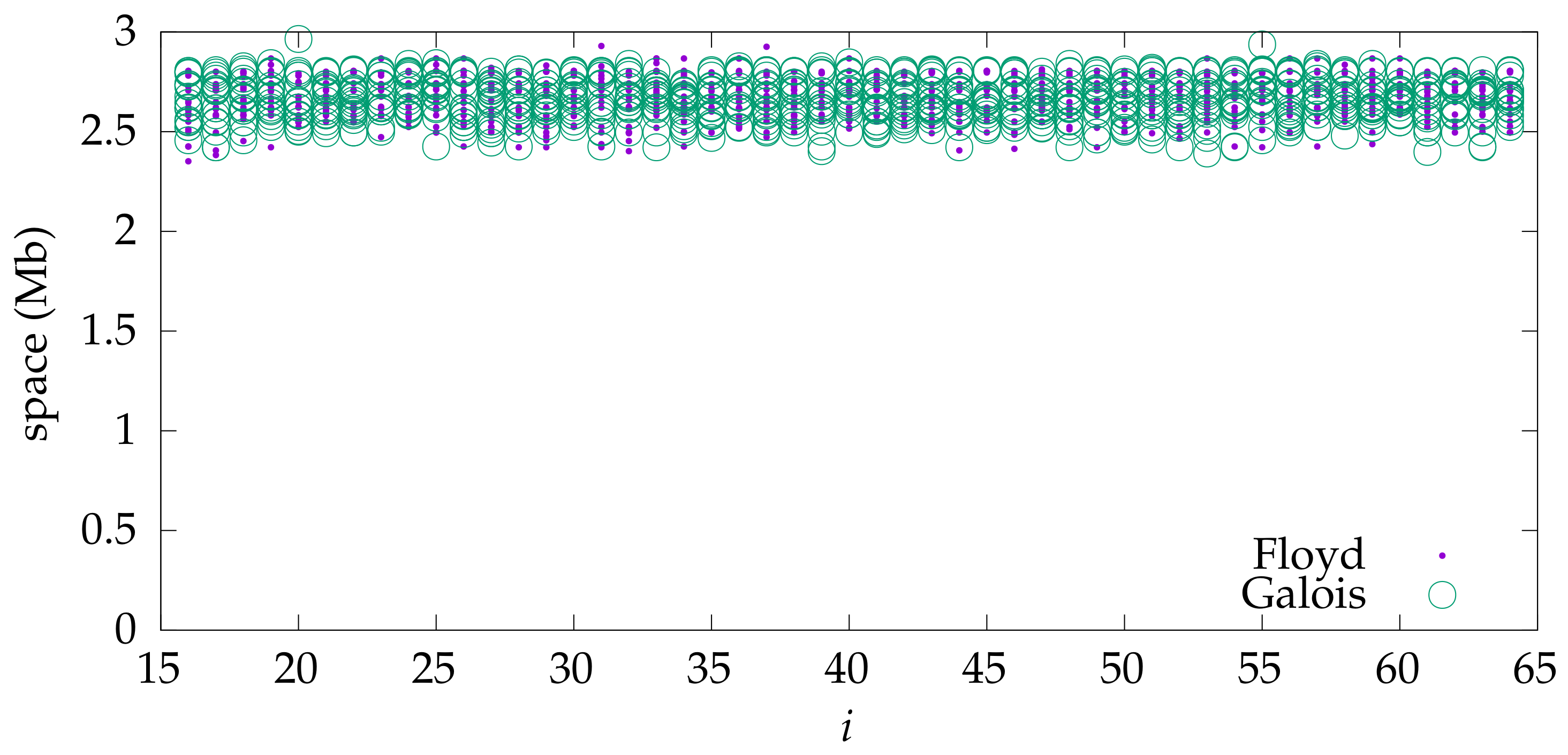
Hence we first setup a sequence of tests to show the improvements provided by Galois’s criteria. We generate a sequence of polynomials for which $m=0$ and n increases. These yield repeating continued fractions of the form $\left[\right(1,\dots ,1,2\left)\right]$, i.e., where all entries of the repeating period are 1, except the last one, which is 2. The experimental results of this experiment are shown in Figure 3 and Figure 4. The space plot of Figure 4 confirms that the space requirements are essentially “constant” as n increases, i.e., are independent from the cycle size. The underlying performance function is not exactly constant and depends on the number of bits in the coefficients of $q\left(x\right)$, i.e., it is $O(1+\log (\max A,B,C,D\left)\right)$ bits. In practice, in this test set, this value is constant. The time plot of Figure 3 confirms that Galois’s criteria are several orders of magnitude faster than the approach based on Floyd’s algorithm. Note that we plotted these result with a logarithmic y scale. Again, the time performance is not completely independent of n, but the impact is very small.

Figure 3. Time performance for fixed $m=0$.

Figure 4. Space performance for fixed $m=0$.

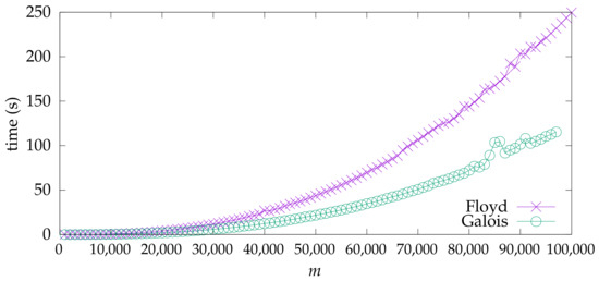
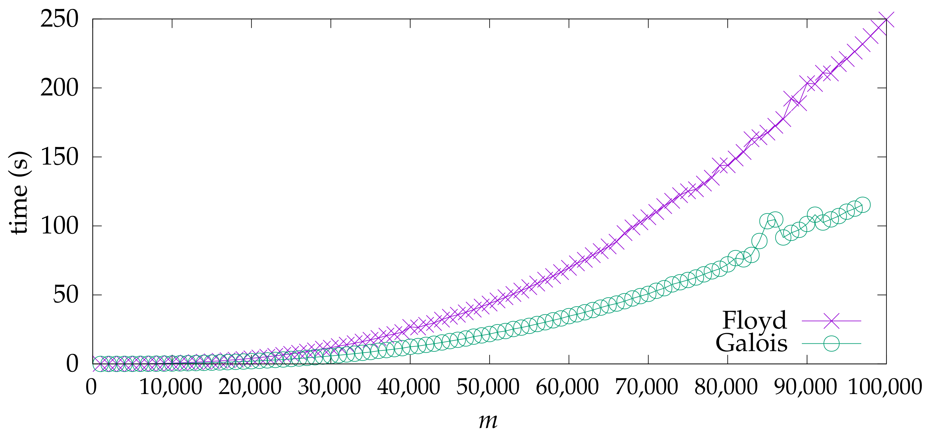
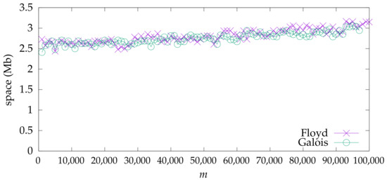
Likewise, to study configurations where the value of m increases and the value of n is always 1, we generate a sequence of polynomials. These generate repeating continued fractions of the form $[1;\dots ,1,(2\left)\right]$, i.e., where there is a big initial sequence of m entries equal to 1 and all entries of the repeating period are 2. The experimental results of this experiment are shown in Figure 5 and Figure 6. The space plot of Figure 6 again reinforces the claim that the space usage is essentially “constant” as m increases. The time plot of Figure 5 again shows that Galois’s criteria are faster. However, in this test case, both algorithms require only $O\left(m\right)$ steps, so the resulting speedup revels the underlying hidden multiplicative factor. This is close to two, as Floyd’s algorithm performs twice the computation as it tracks two states, while Galois criteria only require one such state. Therefore, in this particular plot, we use a linear scale for the y-axis, instead of a logarithmic scale used for the similar case when $m=0$.

Figure 5. Time performance for fixed $n=1$.

Figure 6. Space performance for fixed $n=1$.

Moreover, to further highlight the computational cost of the underlying infinite precision operations, we tested the following continued fractions $[8^{10,000\times i},2;\dots ,1,(8^{10,000\times i},\dots ,$ $8^{10,000\times i},1)]$. In these fractions, both $m=2$ and $n=11$ are fixed, but the size of the underlying integers increases. Inside the repeating portion, most of the coefficients are $8^{10,000\times i}$, except the last one which is 1. The initial prefix consists of another $8^{10,000\times i}$ number followed by a 2. The resulting performance is shown in Figure 7 and Figure 8.

Figure 7. Time performance for fixed $m=2$ and $n=11$.

Figure 8. Space performance for fixed $m=2$ and $n=11$.

As expected in terms of space both algorithms present a very similar performance. But the constant associated with Floyd’s algorithm seems to be larger. This starts to show for very long integers but is not very significant. In terms of time, the difference favors Galois’ criterion much more. Note that $n=11$ is the size of the size, where $m=2$ is the size of the initial prefix. Because Galois’s criterion does not need to traverse the cycle, one would expect the performance difference between these to algorithms to be a factor of around $13/2=6.5$. The experimental factor for $i=100$ is around 6, so the behavior is consistent with the expectation.

Finally, we added some tests where we choose a non-square value for D uniformly at random up to $2^i$. The resulting performance is shown in Figure 9 and Figure 10. The resulting performance is similar to the fixed m tests. The space requirements store only a constant amount of integers whose size does not increase significantly. The time performance shows that Floyd’s algorithm is slower as the value of n should be around $\sqrt{D}\log \left(D\right)$. Recall that according to Theorem 3 the value of m in this data set is always 1.

Figure 9. Time performance for a random value of $D\le 2^i$.

Figure 10. Space performance for a random value of $D\le 2^i$.

5. Related Work

Theorem 1 was famously described and proved by Lagrange [8]. The original proof of the theorem was based on the convergence properties of regular continued fractions. Several other proofs based on similar principles exist, such as the ones from Charves [9] and Hermite [10].

Proofs that do not rely on convergence arguments were given by Ballieu [11], Gonçalves [12], and Perron [13,14]. These proofs make no reference to the convergence of the continued fraction and rely only on the formal algorithm, similar to the one explained in Lemma 1. In the algorithm described by Steinng [15], the sign of $A_i$ was not associated with the size of the zero of the corresponding quadratic polynomials and therefore the resulting cycle of polynomials could be twice as large as the ones we consider. These kinds of proofs are quite direct and require less computation than the earlier ones. A further simplified algorithmic proof was given by Steinng [15]. These proofs are essentially different from the one we present and moreover consider only the sequence of polynomial $q_i\left(x\right)$ and not, explicitly, the sequence of surds $x_i$. An alternative proof, based on Dirichlet groups, is described by Karpenkov [16].

The palindromic structure of the repeating cycle was proven by Galois [17]. A bound on the size of the underlying cycles was proved by Hickerson [4]. This result was further improved by Stanton et al. [2] and Cohn [1], who provided the bound $O\left(\sqrt{D}\log D\right)$. Further studies of the statistical properties of the underlying cycles are also available [3,18].

Recent work on the stability of systems of rational difference equations with Pell coefficients was carried out by Ghe [19]. Also there is an interesting framework relating systems of nonlinear difference equations to generalized Fibonacci sequences given by Salman [20]. Note that the Fibonacci numbers appear as the sequence of cumulants when evaluating the purely periodic continued fraction $\left[\right(1\left)\right]$.

The algorithm for identifying general cycles in minimal space was given by Floyd, according to Knuth [5]. Several other alternatives exist, such as Brent’s algorithm [21], which has the same asymptotic performance as Floyd’s algorithm, but better hidden constants, that can improve experimental performance. Moreover, there is also Gosper’s algorithm. This is a sort of concurrent version of Brent’s algorithm. We chose Floyd’s algorithm as it is simple and requires minimal space and is thus a good alternative to something like a hash table, which also obtains optimal time but requires more space. For a more in-depth discussion of alternative methods consult the survey given by Nivasch [22]. For this specific problem, it is possible to identify in-cycle configurations using Galois’s Criteria [17].

6. Conclusions

We gave a detailed description of the process that is used to obtain the regular periodic continued fraction that represents $\sqrt{D}$, where D is a non-square positive integer. Our description purposely unifies the surd and quadratic polynomial views of the process, as this approach allows us to give simple proofs of the basic properties of the process.

We naturally consider Lagrange’s theorem, which states that this process is bound to repeat. We give a new proof of this result, based only on combinatorial arguments, i.e., without resorting to convergence or analytical arguments.

We implement this process using the infinite precision library GMP. This allows us to experimentally study this process for arbitrarily large values. We consider two approaches to determine which states are initial and which states are part of the loop. Both approaches use only a constant amount of integers. Naive approaches of keeping lists of states were excluded as they would unnecessarily waste space. We consider two approaches, Floyd’s algorithm and Galois’s criteria. Our experimental results showed that Galois’s criteria are clearly the fastest approach.

Our implementation also includes routines to invert the given process, i.e., to determine a degree-two polynomial from a given regular periodic continued fraction. We added a routine to solve Pell’s equation and made the resulting software publicly available.

Several interesting mathematical results are related with this process, particularly, the bound on the size of the resulting loops $O\left(D\log D\right)$. We expect this software can help in the study of this and other related problems. We may consider studying the size of the initial states in relation to the polynomial coefficients, or investigating the alternative cycles associated with a given discriminant D.

References

- Cohn, J. The length of the period of the simple continued fraction of d1/2. Pac. J. Math. 1977, 71, 21–32. [Google Scholar] [CrossRef] [Scilit]
- Stanton, R.; Sudler, C.; Williams, H. An upper bound for the period of the simple continued fraction for . Pac. J. Math. 1976, 67, 525–536. [Google Scholar] [CrossRef] [Scilit][Green Version]
- Battistoni, F.; Grenié, L.; Molteni, G. The first and second moments for the length of the period of the continued fraction expansion for . Mathematika 2024, 70, 4. [Google Scholar] [CrossRef] [Scilit]
- Hickerson, D.R. Length of period simple continued fraction expansion of √d. Pac. J. Math. 1973, 46, 429–432. [Google Scholar] [CrossRef] [Scilit][Green Version]
- Knuth, D.E. The Art of Computer Programming; Seminumerical Algorithms; Exercises 6 and 7; Addison Wesley Longman Publishing Co., Inc.: Reading, MA, USA, 1969; Volume 2, 7p. [Google Scholar]
- Jeffrey, A. Complex Analysis and Applications, 2nd ed.; Taylor & Francis: Oxfordshire, UK, 2005. [Google Scholar]
- Schönhage, A.; Strassen, V. Schnelle Multiplikation großer Zahlen. Computing 1971, 7, 281–292. [Google Scholar] [CrossRef] [Scilit]
- Lagrange, J.-L. Additions au m moire sur la r solution des quations numériques. MéMoires L’AcadéMie R. Sci.-Belles-Lettres 1770, 24. [Google Scholar]
- Charves. Démonstration de la périodicité des fractions continues, engendrées par les racines d’une équation du deuxième degré. Bull. Sci. Math. Astron. 1877, 1, 41–43. [Google Scholar]
- Hermite, C. Sur La Théorie Des Fractions Continues; Cambridge University Press: Cambridge, UK, 2009; pp. 178–180. [Google Scholar]
- Ballieu, R. Sur le développement des irrationnelles quadratiques en fractions continues régulières. Mathesis 1942, 54, 304–314. [Google Scholar]
- Gonçalves, J.V. Sur les fractions continues réelles. Univ. Lisb. Rev. Fac. Ciências 1952, 2, 297–335. [Google Scholar]
- Hlawka, E.; Schoissengeier, J. Zahlentheorie: Eine Einführung; Manz: Vienna, Austria, 1979. [Google Scholar]
- Perron, O. Neue Periodizitätsbeweise für die regelmäßigen und halbregelmäßigen Kettenbrüche quadratischer Irrationalzahlen. Sitzungsber. Bayer. Akad. Wiss. Math.-Naturwiss. Kl. 1955, 1954, 321–333. [Google Scholar]
- Steinig, J. A proof of Lagrange’s theorem on periodic continued fractions. Arch. Math. 1992, 59, 21–23. [Google Scholar] [CrossRef] [Scilit]
- Karpenkov, O.N. Lagrange’s Theorem; Springer: Berlin/Heidelberg, Germany, 2022; pp. 129–138. [Google Scholar]
- Galois, É. Analyse algébrique. Démonstration d’un théorème sur les fractions continues périodiques. In Annales de Mathématiques Pures et Appliquées; Joseph-Diez Gergonne: Nîmes, France, 1828; Volume 19, pp. 294–301. [Google Scholar]
- Aka, M.; Shapira, U. On the evolution of continued fractions in a fixed quadratic field. J. D’Analyse Math. 2018, 134, 335–397. [Google Scholar] [CrossRef] [Scilit]
- Ghezal, A.; Zemmouri, I. Global stability of multi-dimensional system of rational difference equations of higher-order with Pell-coefficients. Bol. Soc. Parana. Mat. 2025, 43, 1–9. [Google Scholar] [CrossRef] [Scilit]
- Al Salman, H.J. Closed-form solutions of systems of nonlinear difference equations and their connections to generalized Fibonacci numbers and related sequences. AIMS Math. 2025, 10, 25307–25328. [Google Scholar] [CrossRef] [Scilit]
- Brent, R.P. An improved Monte Carlo factorization algorithm. BIT 1980, 20, 176–184. [Google Scholar] [CrossRef] [Scilit]
- Nivasch, G. Cycle detection using a stack. Inform. Process. Lett. 2004, 90, 135–140. [Google Scholar] [CrossRef] [Scilit]
Disclaimer/Publisher’s Note: The statements, opinions and data contained in all publications are solely those of the individual author(s) and contributor(s) and not of MDPI and/or the editor(s). MDPI and/or the editor(s) disclaim responsibility for any injury to people or property resulting from any ideas, methods, instructions or products referred to in the content. |
© 2026 by the author. Licensee MDPI, Basel, Switzerland. This article is an open access article distributed under the terms and conditions of the Creative Commons Attribution (CC BY) license.