Redundancy-Suppressed Multi-Objective Evolutionary Algorithm with Validation-Calibrated Archiving for Sea Surface Temperature Sensor Placement

Abstract

The sea surface temperature sparse sensor placement (SST-SSP) problem involves selecting a limited number of in situ observation sites to reconstruct full sea surface temperature fields. We first establish the SST-SSP model, considering proper orthogonal decomposition (POD) information, deployment burden, and modal redundancy. This is different from well-known POD-based solutions. Then, we propose a cost-aware redundancy-suppressed multi-objective evolutionary algorithm based on decomposition (CARS-MOEA/D) to solve this problem. Specifically, CARS-MOEA/D uses redundancy-assisted decomposition search to explore complementary layouts and validation-calibrated external archiving to retain favorable reconstruction-burden trade-offs. Experiments on 36 Optimum Interpolation Sea Surface Temperature (OISST) instances cover eleven regional and basin-scale domains, as well as the global ocean at three spatial resolutions. The results demonstrate that CARS-MOEA/D outperforms state-of-the-art multi-objective evolutionary algorithms. A Tropical Atmosphere Ocean buoy-network case study further illustrates the practical value of CARS-MOEA/D. The official data sources and source-code repository are provided to support reproducible research and future work in this area.

1. Introduction

The sea surface temperature sparse sensor placement (SST-SSP) problem is concerned with selecting a limited set of observation sites for reconstructing complete sea surface temperature (SST) fields. SST observations support climate monitoring [1], data-product validation [2], and regional ocean analysis [3]. Continued ocean warming and marine heatwaves increase the need for sustained observing capability [4,5,6]. In practice, moored-buoy networks are constrained by platform availability, ship time, access windows, communication capacity, and maintenance resources [7]. Observing system experiments provide system-level evidence for network decisions [8], while the Tropical Pacific Observing System redesign emphasizes platform complementarity, sustained records, and robust operation [9]. As the candidate network and allowed sensor number grow, the number of feasible station portfolios increases rapidly. SST-SSP is therefore a difficult combinatorial planning problem that requires efficient reconstruction-oriented screening before field evaluation.

Proper orthogonal decomposition (POD) links sparse observations to full-field reconstruction through a low-dimensional basis [10,11]. Current approaches mainly optimize observability, information volume, or reconstruction stability [12,13,14], subject to constraints such as finite sensor numbers, task specificity, and mobility [15,16,17]. While these models offer effective criteria, information-rich layouts often require numerous stations or remote sites. Additionally, selected sites may produce similar responses across the retained POD modes. In this case, information quality alone does not characterize deployment burden or marginal modal coverage provided by each station. This motivates considering deployment burden and marginal modal coverage in the model.

The proposed SST-SSP model has three objectives. The first objective minimizes the negative log determinant of the selected POD observation matrix, favoring high global information. The second objective combines station count and normalized offshore distance. Each selected site consumes platform and service capacity, and remote access adds vessel effort and operational exposure. The third objective minimizes modal redundancy. Two sites that are informative individually may exhibit similar responses in the retained modes, so selecting both consumes two station slots but adds little modal coverage. Earlier empirical orthogonal function (EOF)-based methods used cross products or exclusion-volume constraints to reduce redundant measurements [18,19]. Since fixed thresholds can have different meanings across regions, resolutions, POD ranks, and sensor numbers, modal redundancy is treated as a graded objective that favors complementary POD responses.

The resulting model has a variable-cardinality binary decision vector and three conflicting objectives. No single layout can minimize all objectives simultaneously, so a set of nondominated layout solutions is required to provide valuable information for decision makers [20,21]. Recently, the decomposition-based multi-objective evolutionary algorithm (MOEA/D) has been shown to be powerful for many multi-objective optimization problems. It distributes the search among scalar subproblems and exchanges information through weight-vector neighborhoods [22]. This decomposition structure is suitable when no trade-off direction is prescribed in advance [23]. These facts motivate a decomposition-based evolutionary search for the SST-SSP problem.

However, information objectives and held-out reconstruction error characterize different aspects of a layout [24,25]. A Pareto archive constructed only in the three-objective search space may retain layouts with unfavorable validation root-mean-square error (RMSE), whereas evaluating every offspring by full-field reconstruction would substantially increase the search cost. To address this mismatch, we propose a cost-aware redundancy-suppressed MOEA/D (CARS-MOEA/D). Redundancy-assisted decomposition search explores complementary layouts across sensor budgets. A validation-calibrated external archive periodically evaluates representative layouts and retains favorable validation-RMSE–burden trade-offs. The independent test set is reserved for final evaluation.

The contributions of this work are summarized as follows.

First, a cost-aware tri-objective SST-SSP model jointly represents POD information, region-normalized deployment burden, and modal redundancy. The same formulation supports prospective site planning and retention decisions for existing networks.

Second, CARS-MOEA/D combines redundancy-assisted decomposition search with validation-calibrated external archiving. The search component promotes complementary layouts, while the archive component converts the explored objective trade-offs into reconstruction-oriented decisions.

Third, the method is evaluated on 36 Optimum Interpolation Sea Surface Temperature (OISST) instances for Pareto quality, reconstruction accuracy, scalability, component effectiveness, and robustness. A Tropical Atmosphere Ocean (TAO) buoy-network case further examines station retention, criticality, and backup-site selection under historical missingness.

The rest of this paper is organized as follows. Section 2 describes the POD-based SST reconstruction model and formulates the tri-objective sensor placement problem. Section 3 presents the proposed CARS-MOEA/D method. Section 4 reports the experimental settings, parameter analysis, algorithm comparisons, ablation studies, and engineering assessments. Finally, Section 5 concludes this paper and suggests future research directions.

2. Problem Formulation

The cost-aware SST-SSP model combines a cardinality-constrained layout, POD reconstruction, three placement objectives, and validation-based decision selection.

2.1. Problem Description

The SST field in a selected oceanic region is divided into valid ocean grid points. The notation used throughout the paper is listed in Table 1. Symbols used within a single equation or algorithm are defined when introduced. The problem is formulated below using this notation.

Table 1. Main notation used throughout the paper.

Symbol	Meaning
$\mathsf{\Omega },P$	Candidate-site set and its number of valid sites.
$\mathit{b},X,\mathcal{S}$	Binary layout vector, selected sensor set, and feasible solution space.
$K_{min},K_{max},K$	Lower and upper sensor-number bounds, and layout cardinality (a fixed sensor budget where specified).
${\mathit{x}}_t,\overline{\mathit{x}}$	SST snapshot at time t and the training-period mean field.
${\mathcal{D}}_{\mathrm{tr}},{\mathcal{D}}_{\mathrm{val}},{\mathcal{D}}_{\mathrm{test}},T_{\mathrm{tr}}$	Training, validation, and temporally held-out test sets, and number of training snapshots.
${\tilde{\mathit{X}}}_{\mathrm{tr}},\mathit{U},\mathsf{\Sigma },\mathit{V}$	Centered training matrix and its singular-value-decomposition factors.
$\mathsf{\Phi },{\mathit{\varphi }}_i,r,r_{min},r_{max},\eta$	POD basis, its ith row, retained rank and bounds, and explained-variance threshold.
$C_X,{\mathsf{\Psi }}_X$	Row-selection matrix and POD observation matrix $C_X\mathsf{\Phi }$.
${\mathit{y}}_t,{\mathit{a}}_t,{\widehat{\mathit{x}}}_t$	Sparse observations, estimated POD coefficients, and reconstructed field.
$\rho ,I,ϵ$	Ridge coefficient, identity matrix, and positive numerical safeguard.
${\mathsf{\Omega }}_{\mathrm{land}},({\phi }_i,{\ell }_i),\overline{\phi },\Delta {\ell }_{iq}$	Land-cell set, latitude–longitude coordinates, regional mean latitude, and periodic longitude separation.
${\delta }_i,{\tilde{\delta }}_i,{\delta }_{min},{\delta }_{max},\gamma$	Offshore distance, its normalization and extrema, and the distance exponent.
${\mathit{u}}_i$	Normalized POD response of candidate site i.
$f_1,f_2,f_3,\mathit{F}$	Information, deployment-burden, redundancy objectives, and their vector.
${RMSE}_{\mathcal{D}}$	Reconstruction RMSE evaluated on snapshot set $\mathcal{D}$.
ND	Nondominated filtering operator.
${\mathcal{A}}_{\mathrm{s}},{\mathcal{A}}_{\mathrm{val}},\mathcal{H}$	Search archive, validation-calibrated external archive, and cumulative validation-RMSE cache.
$N,N_{\mathrm{nb}},G_{max},T_{max}$	Population/search-archive size, weight-neighborhood size, generation limit, and wall-clock limit.
${\tau }_{\mathrm{cal}},N_{\mathrm{cal}},N_{\mathrm{val}}$	Calibration interval, layouts calibrated per event, and external-archive capacity.
$\mathcal{P},\mathcal{Q}$	Current population and offspring set.
$\mathrm{\Lambda },{\mathsf{\lambda }}^i,{\mathcal{B}}^i$	Weight-vector set, its ith vector, and the corresponding neighborhood.
$g^{\mathrm{te}},{\mathit{z}}^{*},{\mathit{z}}^{\mathrm{nad}}$	Tchebycheff scalar function and current ideal and nadir objective vectors.
$h_i,{\kappa }_i,p_c,p_m$	Leverage score, cluster label, crossover rate, and mutation rate.
$R,S$	Normalized common empirical reference front and normalized approximation front returned by an algorithm.
$\mathrm{HV},\mathrm{IGD},\mathrm{GD}$	Hypervolume, inverted generational distance, and generational distance.
$C_{\mathrm{cov}}(S_1,S_2),R_{\mathrm{ND}}$	Pairwise front coverage and nondominated retention rate.
$\mathrm{S}/{\mathrm{N}}_{\mathrm{STB}},\mathrm{S}/{\mathrm{N}}_{\mathrm{LTB}}$	Taguchi signal-to-noise (S/N) ratios for smaller-the-better (STB) and larger-the-better (LTB) responses.

Let $\mathsf{\Omega }=\{1,2,\dots ,P\}$ denote the candidate site set. Depending on the planning task, $\mathsf{\Omega }$ describes prospective ocean cells or the coordinates of an existing buoy network. The task selects observations that retain sufficient SST information under station and access constraints. The POD basis, site-specific burden index, and admissible sensor-number range define the problem inputs. The model returns a portfolio of feasible layouts with different resource–reconstruction trade-offs.

A sensor layout is encoded by $\mathit{b}\in {\{0,1\}}^P$, where $b_i=1$ means that candidate site i is selected. Its sensor set and the feasible cardinality-constrained solution space are jointly defined by

$$\begin{array}{cc}\hfill X\left(\mathit{b}\right)& =\{i\in \mathsf{\Omega }:b_i=1\},\hfill \end{array}$$

(1)

$$\begin{array}{cc}\hfill \mathcal{S}& =\left\{\mathit{b}\in {\{0,1\}}^P:K_{min}\le \left|X\left(\mathit{b}\right)\right|\le K_{max}\right\}.\hfill \end{array}$$

(2)

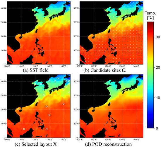
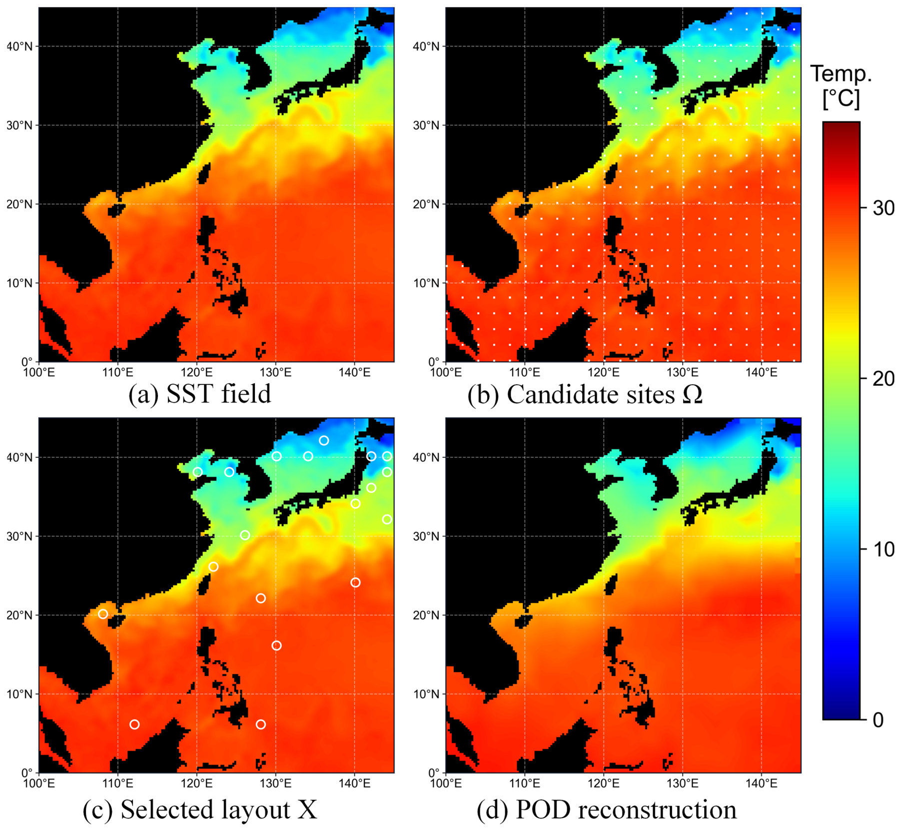
Figure 1 illustrates the connections between the discrete layout and the physical reconstruction process. Panels (a) and (b) show an SST snapshot over the study region and its valid candidate sites, respectively. Panel (c) shows the layout selected by the binary vector $\mathit{b}$. Sampling the snapshot at these sites gives ${\mathit{y}}_t=C_X{\mathit{x}}_t$, from which the POD reconstruction in panel (d) is obtained.

Figure 1. Definition of sea surface temperature sparse sensor placement (SST-SSP) on the small-scale China Sea instance. (a) Sea surface temperature (SST) snapshot ${\mathit{x}}_t$; (b) candidate set $\mathsf{\Omega }$; (c) selected layout $X\subseteq \mathsf{\Omega }$; and (d) proper orthogonal decomposition (POD) reconstruction ${\widehat{\mathit{x}}}_t\left(X\right)$. White squares and open circles mark candidate and selected sites, respectively. Dashed lines are graticules, black denotes land or invalid cells, and one temperature scale is used throughout.

2.2. POD-Based Reconstruction Representation

POD provides the low-dimensional link between sparse observations and the full SST field. Following the standard POD-based sparse-reconstruction setting [10,11], let ${\mathit{x}}_t\in {\mathbb{R}}^P$ denote the SST snapshot at time t. For the $T_{\mathrm{tr}}$ training snapshots, let $\overline{\mathit{x}}$ be their temporal mean and stack ${({\mathit{x}}_t-\overline{\mathit{x}})}^{\top }$ as the rows of the centered matrix ${\tilde{\mathit{X}}}_{\mathrm{tr}}$. Its singular value decomposition separates dominant spatial patterns from their temporal amplitudes:

$$\begin{array}{cc}\hfill {\tilde{\mathit{X}}}_{\mathrm{tr}}& =\mathit{U}\mathsf{\Sigma }{\mathit{V}}^{\top },\hfill \end{array}$$

(3)

$$\begin{array}{cc}\hfill \mathsf{\Phi }& ={\mathit{V}}_{:,1:r}\in {\mathbb{R}}^{P\times r}.\hfill \end{array}$$

(4)

The retained rank r is the smallest rank whose squared singular values explain at least the prescribed fraction $\eta$ of training variability, clipped to $[r_{min},r_{max}]$ and the available matrix rank. Each row of $\mathsf{\Phi }$ is therefore the retained modal response of one candidate site. For a selected sensor set X, let $C_X$ be its row-selection matrix. The observation matrix, sparse measurement, ridge estimate, and reconstructed field form the chain

$$\begin{array}{cc}\hfill {\mathsf{\Psi }}_X& =C_X\mathsf{\Phi },\hfill \end{array}$$

(5)

$$\begin{array}{cc}\hfill {\mathit{y}}_t& =C_X{\mathit{x}}_t,\hfill \end{array}$$

(6)

$$\begin{array}{cc}\hfill {\mathit{a}}_t\left(X\right)& ={\left({\mathsf{\Psi }}_X^{\top }{\mathsf{\Psi }}_X+\rho I\right)}^{-1}{\mathsf{\Psi }}_X^{\top }\left({\mathit{y}}_t-C_X\overline{\mathit{x}}\right),\hfill \end{array}$$

(7)

$$\begin{array}{cc}\hfill {\widehat{\mathit{x}}}_t\left(X\right)& =\overline{\mathit{x}}+\mathsf{\Phi }{\mathit{a}}_t\left(X\right).\hfill \end{array}$$

(8)

where ${\mathsf{\Psi }}_X\in {\mathbb{R}}^{\left|X\right|\times r}$ contains the modal responses available at the selected sites and $\rho >0$ is a small ridge coefficient. Thus, the layout determines the sampled modal rows and, through them, the stability and accuracy of full-field reconstruction.

2.3. Tri-Objective Sensor Placement Formulation

Each feasible layout is evaluated from three complementary perspectives. The first objective measures whether the selected POD rows support stable coefficient estimation, the second quantifies the station and offshore-access burden of the selected sites, and the third identifies repeated modal responses as an additional dimension of layout quality. All three objectives are formulated for minimization. The first two define the planning trade-off ultimately returned to the decision maker, whereas $f_3$ is termed auxiliary because it guides candidate generation toward layouts with complementary POD responses.

2.3.1. POD Information Objective

The first requirement is that the selected rows collectively observe the retained POD subspace. The Gram matrix ${\mathsf{\Psi }}_X^{\top }{\mathsf{\Psi }}_X$ summarizes this joint observability, and its determinant provides a D-optimal information-volume criterion for sensor selection [24,25,26]. Converting determinant maximization into the common minimization form gives

$$f_1\left(X\right)=-logdet\left({\mathsf{\Psi }}_X^{\top }{\mathsf{\Psi }}_X+\rho I\right).$$

(9)

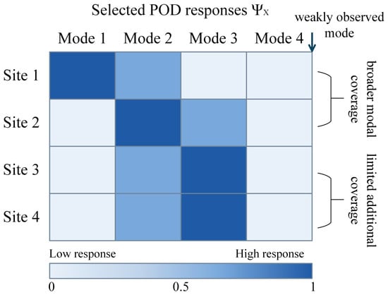
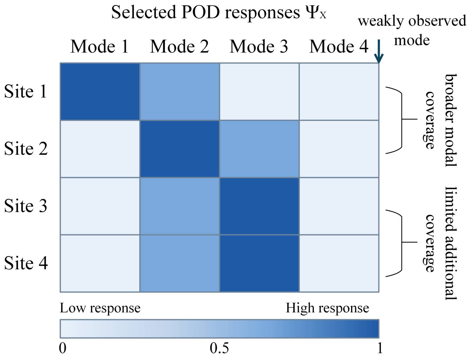
The interpretation of this objective is illustrated in Figure 2. Each row of ${\mathsf{\Psi }}_X$ records the retained-mode responses at one selected site. Each column describes how strongly the complete layout observes one mode. The displayed intensities represent normalized absolute response magnitudes, while the actual POD entries retain their signs. A weak column, illustrated by Mode 4, indicates a poorly observed direction of the retained subspace. Rows with complementary patterns expand the jointly observed modal subspace. Near-duplicate rows add comparatively little information.

Figure 2. Schematic interpretation of the POD information objective for a selected layout X. Rows and columns of ${\mathsf{\Psi }}_X$ correspond to selected sites and retained POD modes, respectively. Darker cells denote larger normalized absolute response magnitudes. Complementary site responses broaden modal coverage, near-duplicate responses add limited new information, and a weakly observed mode contracts the information volume measured by $det({\mathsf{\Psi }}_X^{\top }{\mathsf{\Psi }}_X+\rho I)$.

Algebraically, $det({\mathsf{\Psi }}_X^{\top }{\mathsf{\Psi }}_X+\rho I)$ is the product of the regularized eigenvalues of the Gram matrix. A weakly observed direction produces a small eigenvalue and contracts this information volume. The ridge term $\rho I$ keeps the criterion well-defined for rank-deficient or poorly conditioned layouts. Consequently, a smaller $f_1\left(X\right)$ indicates larger information volume and, generally, a more stable coefficient-estimation problem.

2.3.2. Deployment-Burden Objective

The second objective distinguishes nearshore and remote-ocean layouts by combining a fixed station term with grid-based offshore distance. This formulation quantifies deployment burden consistently across a region. Let ${\mathsf{\Omega }}_{\mathrm{land}}$ contain the land-cell centers in the full-resolution OISST mask, let $({\phi }_i,{\ell }_i)$ and $({\phi }_q,{\ell }_q)$ be the coordinates of ocean site i and land cell q, respectively, and let $\overline{\phi }$ be the regional mean latitude. The periodic longitude separation is

$$\Delta {\ell }_{iq}=min\left\{|{\ell }_i-{\ell }_q|,{360}^{\circ }-|{\ell }_i-{\ell }_q|\right\}.$$

(10)

The offshore distance, its regional normalization, and the layout burden are

$$\begin{array}{cc}\hfill {\delta }_i& =\underset{q\in {\mathsf{\Omega }}_{\mathrm{land}}}{min}\sqrt{{\left[111({\phi }_i-{\phi }_q)\right]}^2+{\left[111cos\left({\displaystyle \frac{\pi \overline{\phi }}{180}}\right)\Delta {\ell }_{iq}\right]}^2},\hfill \end{array}$$

(11)

$$\begin{array}{cc}\hfill {\tilde{\delta }}_i& ={\displaystyle \frac{{\delta }_i-{\delta }_{min}}{{\delta }_{max}-{\delta }_{min}}},\hfill \end{array}$$

(12)

$$\begin{array}{cc}\hfill f_2\left(X\right)& =\sum _{i\in X}\left(1+{\tilde{\delta }}_i^{\gamma }\right),\gamma >0.\hfill \end{array}$$

(13)

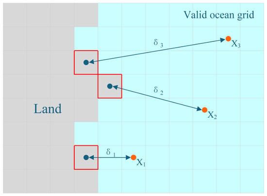
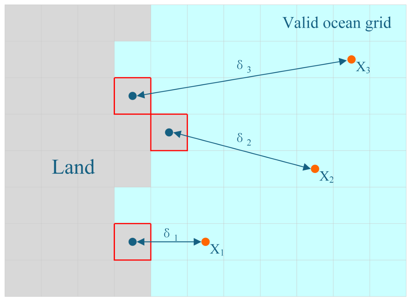
Angular coordinates are in degrees and ${\delta }_i$ is in kilometers; when ${\delta }_{max}={\delta }_{min}$, ${\tilde{\delta }}_i$ is set to zero. The periodic separation in Equation (10) supplies the shorter longitudinal arc across the $0^{\circ }/{360}^{\circ }$ boundary. The raster-index approximation converts latitude to approximately 111 km per degree and scales longitude by the regional mean latitude $\overline{\phi }$, yielding a reproducible within-domain burden index. Figure 3 illustrates how the raster land–sea mask converts a selected ocean cell into a nearest-land distance and then into a site burden. The schematic uses cell centers to match the gridded OISST mask used in the formal experiments.

Figure 3. Grid-based definition of the deployment-burden objective. Gray and cyan cells denote land and valid ocean cells, respectively. Orange circles indicate three illustrative selected sites, whereas blue circles and red outlines mark the centers and extents of their nearest land cells. The double-headed segments represent the center-to-center distances ${\delta }_1$, ${\delta }_2$, and ${\delta }_3$.

The unit term represents the burden associated with one station, while the normalized distance term represents additional offshore access; $\gamma =1$ is used unless stated otherwise. Hence, $f_2$ increases with both sensor number and relative distance from land and provides a consistent within-domain deployment-burden index.

2.3.3. Modal-Redundancy Auxiliary Objective

The determinant in $f_1$ measures global observability, but layouts with similar information volumes may still contain locally repeated modal responses. Let ${\mathit{\varphi }}_i^{\top }$ be the ith row of $\mathsf{\Phi }$. Its normalized response and the average worst-case pairwise similarity of a layout are

$$\begin{array}{cc}\hfill {\mathit{u}}_i& ={\displaystyle \frac{{\mathit{\varphi }}_i}{max\left(\parallel {\mathit{\varphi }}_i{\parallel }_2,ϵ\right)}},\hfill \end{array}$$

(14)

$$\begin{array}{cc}\hfill f_3\left(X\right)& ={\displaystyle \frac{1}{\left|X\right|}}\sum _{i\in X}\underset{\begin{array}{c}j\in X\\ j\ne i\end{array}}{max}\left|{\mathit{u}}_i^{\top }{\mathit{u}}_j\right|,\left|X\right|\ge 2.\hfill \end{array}$$

(15)

Here, $ϵ$ is a positive safeguard and $|{\mathit{u}}_i^{\top }{\mathit{u}}_j|\in [0,1]$ is the modal similarity between two sites; $f_3=0$ for a singleton layout. Larger values indicate stronger repeated responses, so minimizing $f_3$ supplies an auxiliary modal-complementarity direction alongside the primary information–burden trade-off. Because maximum similarity can increase with sensor cardinality K, the independent contribution of $f_3$ is assessed through fixed-K comparisons in Section 4.5.

With $f_m\left(\mathit{b}\right)=f_m\left(X\left(\mathit{b}\right)\right)$, the complete model is

$$\underset{\mathit{b}\in \mathcal{S}}{min}\mathit{F}\left(\mathit{b}\right)=\left(f_1\left(\mathit{b}\right),f_2\left(\mathit{b}\right),f_3\left(\mathit{b}\right)\right).$$

(16)

Standard minimization-based Pareto dominance returns a portfolio of trade-off layouts.

2.4. Validation-Based Decision Criterion

The information objective $f_1$ guides efficient combinatorial search, and validation RMSE measures realized reconstruction on pre-test snapshots. Because $f_1$ depends only on the selected POD rows, it is substantially cheaper to evaluate than reconstructing all validation snapshots. Validation RMSE is therefore applied to a bounded set of candidate layouts during archive calibration. For a snapshot set $\mathcal{D}$, define

$${RMSE}_{\mathcal{D}}\left(X\right)={\displaystyle \frac{1}{\left|\mathcal{D}\right|}}\sum _{{\mathit{x}}_t\in \mathcal{D}}\sqrt{{\displaystyle \frac{1}{P}}{∥{\mathit{x}}_t-{\widehat{\mathit{x}}}_t\left(X\right)∥}_2^2}.$$

(17)

For $\mathcal{D}={\mathcal{D}}_{\mathrm{val}}$, this quantity is denoted by ${RMSE}_{\mathrm{val}}$. Among candidate layouts evaluated on the validation set, preference is defined by Pareto dominance in $({RMSE}_{\mathrm{val}},f_2)$, thereby retaining the reconstruction–burden trade-off in the returned decisions. The capacity-bounded realization of this criterion is described in Section 3.3. Once the validation-based decisions are fixed, they are evaluated on the temporally held-out test set using ${RMSE}_{\mathrm{test}}\equiv {RMSE}_{{\mathcal{D}}_{\mathrm{test}}}$.

3. CARS-MOEA/D Algorithm

CARS-MOEA/D combines tri-objective decomposition search with a validation-calibrated external archive. The former explores information–burden–redundancy trade-offs, whereas the latter retains reconstruction–burden portfolios.

3.1. General Scheme

Let N, $N_{\mathrm{nb}}$, $G_{max}$, and $T_{max}$ denote the population size, neighborhood size, generation limit, and wall-clock limit. External refinement is controlled by interval ${\tau }_{\mathrm{cal}}$, per-event sample count $N_{\mathrm{cal}}$, and archive capacity $N_{\mathrm{val}}$. CARS-MOEA/D maintains population $\mathcal{P}$, a search archive ${\mathcal{A}}_{\mathrm{s}}$ in $(f_1,f_2,f_3)$, and a validation-calibrated external archive ${\mathcal{A}}_{\mathrm{val}}$ in $({RMSE}_{\mathrm{val}},f_2)$. The two archives serve evolutionary search and returned-decision selection, respectively. The overall workflow is summarized in Algorithm 1.

Algorithm 1 Main framework of CARS-MOEA/D.

Input: POD basis $\mathrm{\Phi }$, normalized offshore distances $\left\{{\tilde{\delta }}_i\right\}$, validation set ${\mathcal{D}}_{\mathrm{val}}$, $K_{min}$, $K_{max}$, N, $G_{max}$, $T_{max}$, ${\tau }_{\mathrm{cal}}$, $N_{\mathrm{cal}}$, and $N_{\mathrm{val}}$

Output: Search archive ${\mathcal{A}}_{\mathrm{s}}$ and validation-calibrated external archive ${\mathcal{A}}_{\mathrm{val}}$

1: Construct $\left\{{\mathit{u}}_i\right\}$, leverage scores $\left\{h_i\right\}$, cluster labels $\left\{{\kappa }_i\right\}$, and $\mathit{F}=(f_1,f_2,f_3)$   2: Generate weight vectors $\mathrm{\Lambda }=\{{\mathit{\lambda }}^1,\dots ,{\mathit{\lambda }}^N\}$ and neighborhoods $\left\{{\mathcal{B}}^i\right\}$   3: $\mathcal{P}\leftarrow$ RandomFeasibleInitialization$(K_{min},K_{max},N)$   4: Evaluate $\mathcal{P}$ and initialize ${\mathcal{A}}_{\mathrm{s}}\leftarrow$ EnvironmentalSelect$(\mathcal{P},N)$   5: ${\mathcal{A}}_{\mathrm{val}}\leftarrow ⌀$, $\mathcal{H}\leftarrow ⌀$; initialize the objective cache   6: for $\nu =1$ to $G_{max}$ do   7:     if elapsed wall-clock time reaches $T_{max}$ then   8:         break   9:     end if 10:     Update the ideal and nadir points from $\mathcal{P}$ 11:     $(\mathcal{P},\mathcal{Q})\leftarrow$ DecompositionSearch$(\mathcal{P},\mathrm{\Lambda },\left\{{\mathcal{B}}^i\right\},\mathit{h},\mathsf{\kappa })$ 12:     ${\mathcal{A}}_{\mathrm{s}}\leftarrow$ EnvironmentalSelect$({\mathcal{A}}_{\mathrm{s}}\cup \mathcal{P}\cup \mathcal{Q},N)$ 13:     if $\nu mod{\tau }_{\mathrm{cal}}=0$ then 14:         ${\mathcal{A}}_{\mathrm{val}}\leftarrow$ CalibrateArchive$({\mathcal{A}}_{\mathrm{s}},{\mathcal{D}}_{\mathrm{val}},N_{\mathrm{cal}},N_{\mathrm{val}},\mathcal{H})$ 15:     end if 16: end for 17: ${\mathcal{A}}_{\mathrm{s}}\leftarrow {ND}_{(f_1,f_2,f_3)}({\mathcal{A}}_{\mathrm{s}}\cup \mathcal{P})$ 18: Perform one final external-archive refinement for unevaluated representatives when the remaining budget permits 19: return ${\mathcal{A}}_{\mathrm{s}}$ and ${\mathcal{A}}_{\mathrm{val}}$

The search archive uses inexpensive objective evaluations to drive evolution. The external archive applies validation reconstruction to selected candidates. Initial sensor numbers are drawn uniformly from $[K_{min},K_{max}]$ to cover the admissible network sizes. Sorted sensor-index tuples serve as cache keys for repeated layouts.

3.2. Redundancy-Assisted Decomposition Search

The core search assigns one layout to each weight vector ${\mathsf{\lambda }}^i$ on the three-objective simplex. The $N_{\mathrm{nb}}$ nearest weight vectors form neighborhood ${\mathcal{B}}^i$. Because the objectives have different ranges, replacement uses the normalized Tchebycheff function

$$g^{\mathrm{te}}(X\mid {\mathsf{\lambda }}^i,{\mathit{z}}^{*},{\mathit{z}}^{\mathrm{nad}})=\underset{m\in \{1,2,3\}}{max}\left\{max({\lambda }_m^i,{10}^{-3}){\displaystyle \frac{|f_m\left(X\right)-z_m^{*}|}{max(z_m^{\mathrm{nad}}-z_m^{*},{10}^{-12})}}\right\},$$

(18)

where ${\mathit{z}}^{*}$ and ${\mathit{z}}^{\mathrm{nad}}$ are the current ideal and nadir points. Normalization prevents an objective with a larger numerical range from dominating replacement. The simplex contains boundary and interior weight vectors, so different subproblems emphasize information, burden, redundancy, or their combinations; no single fixed weighting is imposed on the complete population. In particular, information-oriented subproblems remain active when the sensor budget is small, while redundancy-oriented subproblems introduce complementary alternatives. The term auxiliary describes the downstream role of $f_3$: it participates fully in candidate generation, but layouts returned for deployment are selected by the validation-RMSE–burden archive in Section 3.3. Section 4.5 evaluates this design at fixed sensor cardinality to separate the contribution of $f_3$ from changes in network size.

The set operators use a fixed structure extracted from the POD basis and candidate coordinates. Candidate site i has leverage score $h_i={\parallel {\mathit{\varphi }}_i\parallel }_2^2$ [11], and K-means labels ${\kappa }_i$ are computed once from standardized latitude, sine and cosine of longitude, and the first $min(5,r)$ POD components [27]. Set crossover samples from the parental union and fill missing sites with probability proportional to $h_i/(1+n_{{\kappa }_i})$, where $n_{{\kappa }_i}$ counts selected sites in cluster ${\kappa }_i$. Add, remove, and swap mutation moves are selected with probabilities 0.2, 0.2, and 0.6, respectively; the higher swap probability favors spatial refinement at fixed cardinality, while balanced add and remove moves explore the admissible sensor-number range.

Algorithm 2 allows an offspring to update several neighboring subproblems when it improves their scalarized values, so one complementary layout can benefit nearby trade-off directions.

Algorithm 2 Redundancy-assisted MOEA/D decomposition search.

Input: Population $\mathcal{P}$, weight vectors $\mathrm{\Lambda }$, neighborhoods $\left\{{\mathcal{B}}^i\right\}$, scores $\mathit{h}$, labels $\mathsf{\kappa }$, rates $p_c,p_m$

Output: Offspring set $\mathcal{Q}$ and updated population $\mathcal{P}$

1: $\mathcal{Q}\leftarrow ⌀$; update ${\mathit{z}}^{*}$ and ${\mathit{z}}^{\mathrm{nad}}$   2: for each subproblem i in random order do   3:     Select two parents $X^{p_1}$ and $X^{p_2}$ from ${\mathcal{B}}^i$   4:     if $rand<p_c$ then   5:         Draw $K^c\sim Unif\{K_{min},\dots ,K_{max}\}$ and form $X^c$ from $X^{p_1}\cup X^{p_2}$   6:         Fill missing sites using $\mathit{h}$ and $\mathsf{\kappa }$   7:     else   8:         $X^c\leftarrow X^{p_1}$   9:     end if 10:     if $rand<p_m$ then 11:         Apply an add, remove, or swap move to $X^c$ and enforce $K_{min}\le \left|X^c\right|\le K_{max}$ 12:     end if 13:     Evaluate $\mathit{F}\left(X^c\right)=(f_1,f_2,f_3)$ using the objective cache 14:     Update ${\mathit{z}}^{*}$ and ${\mathit{z}}^{\mathrm{nad}}$ with $\mathit{F}\left(X^c\right)$ 15:     for each $j\in {\mathcal{B}}^i$ do 16:         if $g^{\mathrm{te}}(X^c\mid {\mathit{\lambda }}^j,{\mathit{z}}^{*},{\mathit{z}}^{\mathrm{nad}})\le g^{\mathrm{te}}(X^j\mid {\mathit{\lambda }}^j,{\mathit{z}}^{*},{\mathit{z}}^{\mathrm{nad}})$ then 17:            $X^j\leftarrow X^c$ 18:         end if 19:     end for 20:     $\mathcal{Q}\leftarrow \mathcal{Q}\cup \left\{X^c\right\}$ 21: end for 22: return $\mathcal{Q}$ and $\mathcal{P}$

3.3. Validation-Calibrated External Archive Refinement

Algorithm 3 limits validation cost by evaluating at most $N_{\mathrm{cal}}$ unseen layouts every ${\tau }_{\mathrm{cal}}$ generations. Its cumulative archive retains at most $N_{\mathrm{val}}$ layouts in $({RMSE}_{\mathrm{val}},f_2)$.

Algorithm 3 Validation-calibrated external archive refinement.

Input: Search archive ${\mathcal{A}}_{\mathrm{s}}$, validation set ${\mathcal{D}}_{\mathrm{val}}$, per-event sample count $N_{\mathrm{cal}}$, archive capacity $N_{\mathrm{val}}$, RMSE cache $\mathcal{H}$

Output: Updated validation-calibrated external archive ${\mathcal{A}}_{\mathrm{val}}$

1: Rank ${\mathcal{A}}_{\mathrm{s}}$ by three-objective nondominance   2: Within each front, sort layouts by decreasing crowding distance   3: Concatenate the fronts to obtain the representative order $\mathcal{L}$   4: $n_{\mathrm{eval}}\leftarrow 0$   5: for each layout $X\in \mathcal{L}$ do   6:     if $X\notin \mathcal{H}$ and $n_{\mathrm{eval}}<N_{\mathrm{cal}}$ then   7:         Reconstruct all snapshots in ${\mathcal{D}}_{\mathrm{val}}$ and compute ${RMSE}_{\mathrm{val}}\left(X\right)$   8:         Store ${RMSE}_{\mathrm{val}}\left(X\right)$ in $\mathcal{H}$ and set $n_{\mathrm{eval}}\leftarrow n_{\mathrm{eval}}+1$   9:     end if 10:     if $n_{\mathrm{eval}}=N_{\mathrm{cal}}$ then 11:         break 12:     end if 13: end for 14: Form ${\mathcal{C}}_{\mathrm{val}}=\{(X,{RMSE}_{\mathrm{val}}\left(X\right),f_2\left(X\right)):X\in \mathcal{H}\}$ 15: ${\mathcal{A}}_{\mathrm{val}}\leftarrow$ EnvironmentalSelect$({\mathcal{C}}_{\mathrm{val}},N_{\mathrm{val}})$ in $({RMSE}_{\mathrm{val}},f_2)$ 16: return  ${\mathcal{A}}_{\mathrm{val}}$

For one layout containing k sensors and r retained modes, calculating $f_1$ requires forming an $r\times r$ Gram matrix and its log determinant, while $f_3$ requires the pairwise similarities among the k normalized modal rows. The dominant costs are therefore $O(k{r}^2+r^3)$ and $O\left(k^{2}r\right)$, respectively. For one newly calibrated layout, reconstruction over $|{\mathcal{D}}_{\mathrm{val}}|$ validation snapshots and P ocean cells additionally costs approximately $O\left(|{\mathcal{D}}_{\mathrm{val}}|(kr+r^2+Pr)\right)$ after the layout-specific least-squares factors are formed. At most $N_{\mathrm{cal}}$ new layouts incur this cost at one calibration event. The objective and RMSE caches reduce repeated work, and the calibration budget bounds the number of validation reconstructions per event. Because the reconstruction term grows linearly with P after the layout-specific factors are formed, periodic bounded calibration is most consequential on basin-scale and global instances. Empirical growth with P and k is reported in Section 4.6.2.

4. Results and Discussion

4.1. Experimental Setup

The experiments use the daily mean SST variable of the National Oceanic and Atmospheric Administration (NOAA) OISST version 2.1 from 2010 to 2025 [1]. Starting from the first daily field in each annual file, every seventh time index is retained, giving 53 snapshots per year. The snapshots from 2010–2018, 2019–2021, and 2022–2025 form the training, validation, and temporally held-out test sets, respectively. The three sets contain 477, 159, and 212 snapshots. The training set determines the POD basis and its retained rank. The rank is the smallest value explaining at least 95% of training variance within $[20,50]$. The effect of relaxing the upper rank bound on the large global instance is examined in Section 4.6.4. The calibrated archive in Section 3.3 uses the validation set, and the test set supplies the final evaluation. (The NOAA OISST v2.1 data used to construct the test instances are publicly available from the https://www.ncei.noaa.gov/products/optimum-interpolation-sst (accessed on 17 May 2026); the TAO buoy observations used in the engineering case are available from the https://tao.ndbc.noaa.gov/tao/data_download/ (accessed on 16 July 2026)).

OISST is a Level-4 blended analysis constructed from satellite and in situ observations with spatial interpolation [1]. The temporal split isolates a held-out period and evaluates reconstruction of the OISST analysis product under a fixed historical POD basis. Section 4.7 then evaluates transfer with recorded in situ observations and historical missingness from the TAO network.

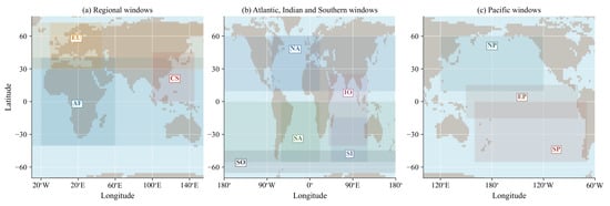
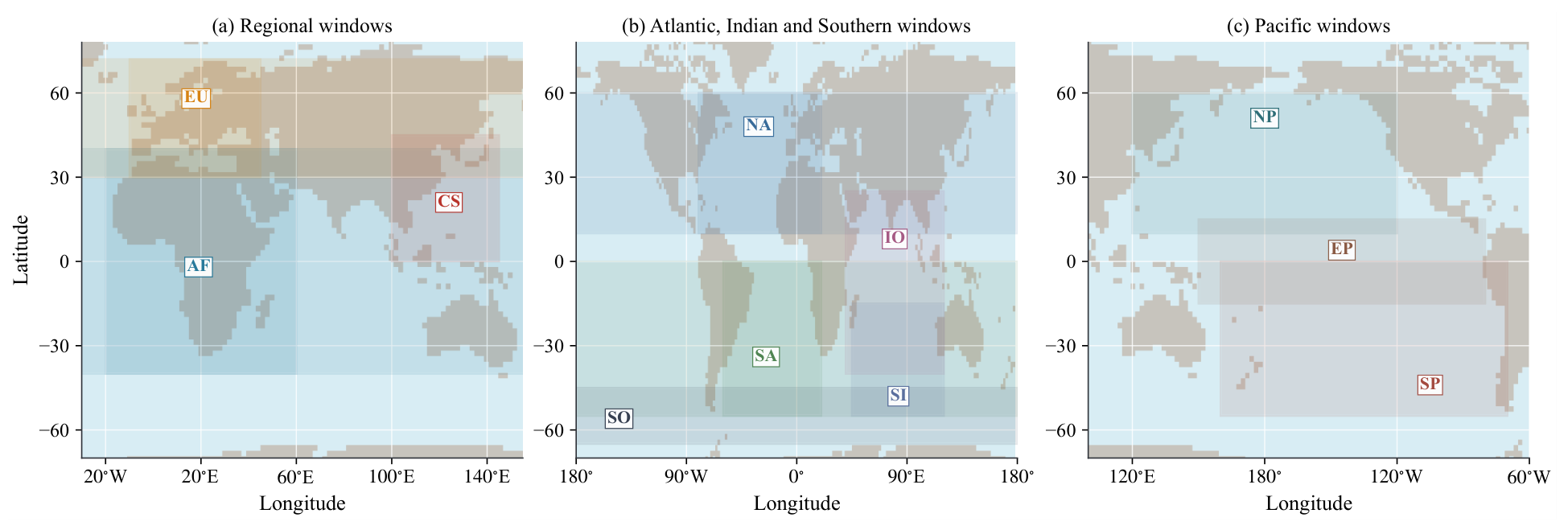
Twelve oceanic domains are considered. The coordinate windows are China Sea (0–${45}^{\circ }$ N, 100–${145}^{\circ }$ E), African waters (${40}^{\circ }$ S–${40}^{\circ }$ N, ${20}^{\circ }$ W–${60}^{\circ }$ E), European waters (30–${72}^{\circ }$ N, ${10}^{\circ }$ W–${45}^{\circ }$ E), North Atlantic (10–${60}^{\circ }$ N, ${80}^{\circ }$ W–${20}^{\circ }$ E), South Atlantic (${55}^{\circ }$ S–$0^{\circ }$, ${60}^{\circ }$ W–${20}^{\circ }$ E), North Pacific (10–${60}^{\circ }$ N, ${120}^{\circ }$ E–${120}^{\circ }$ W), South Pacific (${55}^{\circ }$ S–$0^{\circ }$, ${160}^{\circ }$ E–${70}^{\circ }$ W), Indian Ocean (${40}^{\circ }$ S–${25}^{\circ }$ N, 40–${120}^{\circ }$ E), South Indian Ocean (55–${15}^{\circ }$ S, 45–${120}^{\circ }$ E), Equatorial Pacific (${15}^{\circ }$ S–${15}^{\circ }$ N, ${150}^{\circ }$ E–${80}^{\circ }$ W), and Southern Ocean (65–${45}^{\circ }$ S, all longitudes). Longitude-wrapping windows are assembled before the valid-ocean mask is applied. The global domain uses all valid OISST ocean cells and is therefore not represented by another rectangle in Figure 4.

Figure 4. Spatial coverage of the eleven regional and basin-scale OISST coordinate windows. (a) African waters (AF), European waters (EU), and China Sea (CS); (b) North Atlantic (NA), South Atlantic (SA), Indian Ocean (IO), South Indian Ocean (SI), and Southern Ocean (SO); and (c) North Pacific (NP), South Pacific (SP), and Equatorial Pacific (EP). Only valid ocean cells inside each window enter the corresponding instance. The global domain uses all valid OISST ocean cells and is not outlined separately.

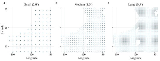
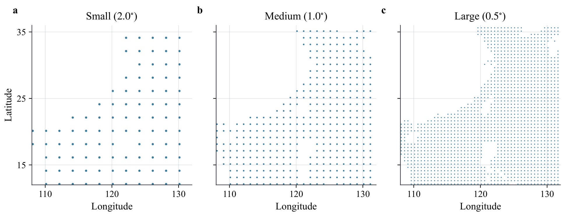
The three spatial resolutions are obtained by direct coordinate subsampling of the native ${0.25}^{\circ }$ grid with strides 8, 4, and 2, yielding ${2.0}^{\circ }$, ${1.0}^{\circ }$, and ${0.5}^{\circ }$ candidate grids; no block averaging is applied. Cells with invalid SST values under the OISST land–sea mask are excluded. As summarized in Table 2, the resulting 36 instances range from 231 candidate sites in the small European instance to 172,681 sites in the large global instance. Figure 5 illustrates the corresponding change in candidate-grid density within the same China Sea subregion. This range evaluates the method across local, basin-scale, and global search spaces. Within each geographical domain, the small, medium, and large instances are nested coordinate subsamples of the same temporally split OISST fields rather than three independent ocean-temperature data sets. They are treated as distinct optimization instances because their candidate sets, POD bases, and search spaces differ; algorithm runs and random seeds are independent across every domain–scale combination.

Table 2. Spatial scales and search settings of the formal instances.

Scale	Grid Spacing	Candidate Sites	Sensor-Number Range	POD Rank
Small	${2.0}^{\circ }$	231–10,741	5–40	20–50
Medium	${1.0}^{\circ }$	941–43,063	5–80	20–50
Large	${0.5}^{\circ }$	3761–172,681	10–160	20–50

Figure 5. Candidate ocean cells in the same China Sea subregion at (a) small, (b) medium, and (c) large spatial scales, corresponding to grid spacings of ${2.0}^{\circ }$, ${1.0}^{\circ }$, and ${0.5}^{\circ }$, respectively.

Five evolutionary methods are included in the main comparison. NSGA-II uses nondominated sorting and crowding distance to balance convergence and diversity [28]. MOPSO maintains personal-best states and samples leaders from a nondominated external archive [29]. Conventional MOEA/D decomposes the tri-objective problem into normalized Tchebycheff subproblems connected by weight-vector neighborhoods [22]. Compact calibrated MOEA/D is a mechanism-based comparison method constructed during this study rather than a previously published algorithm. It integrates graph-guided initialization, probability-based search guidance, and local improvement, which showed comparatively effective search performance in the preliminary experiments. It is therefore included as an enhanced comparison method. CARS-MOEA/D instead uses the proposed redundancy-assisted decomposition search and cumulative validation-calibrated archive described in Section 3.

All five methods use the same binary subset encoding, sensor-number bounds, three objective definitions, population size $N=40$, and instance-specific wall-clock budget. Their algorithm-specific selection and update rules remain unchanged. The wall-clock budget includes all objective-evaluation and external-refinement costs of CARS-MOEA/D. Larger regions receive longer budgets because the cost of evaluating a layout grows with the number of valid ocean cells. The budgets are listed in Table 4. Every algorithm–instance combination is independently repeated 21 times using seeds 1–21. Table 3 summarizes the algorithm-specific settings.

Table 3. Principal algorithm-specific settings used in the formal comparison. Common settings are $N=40$, $p_m=0.9$, the same objectives and bounds, seeds 1–21, and the wall-clock budgets in Table 4.

Method	Core Search Rule	Initialization and Guidance	Archive or Refinement
NSGA-II	Nondominated sorting; crowding distance	Random feasible; set crossover; add/remove/swap mutation	Population selection
MOPSO	Personal-best and nondominated leader	Random feasible; state weights 0.45/0.25/0.30	Leader archive (capacity: 40)
MOEA/D	Normalized Tchebycheff; $N_{\mathrm{nb}}=8$	Random feasible; union-set crossover; add/remove/swap mutation	Weight-vector population
Compact calibrated MOEA/D	Normalized Tchebycheff; $N_{\mathrm{nb}}=8$	Graph initialization; probability guidance; local search 0.10	Validation-calibrated archive
CARS-MOEA/D	Normalized Tchebycheff; $N_{\mathrm{nb}}=8$	Random feasible; add/remove/swap mutation	Search archive 40; ${\tau }_{\mathrm{cal}}=30$, $N_{\mathrm{cal}}=32$, $N_{\mathrm{val}}=80$

Table 3. Principal algorithm-specific settings used in the formal comparison. Common settings are $N=40$, $p_m=0.9$, the same objectives and bounds, seeds 1–21, and the wall-clock budgets in Table 4.

Method	Core Search Rule	Initialization and Guidance	Archive or Refinement
NSGA-II	Nondominated sorting; crowding distance	Random feasible; set crossover; add/remove/swap mutation	Population selection
MOPSO	Personal-best and nondominated leader	Random feasible; state weights 0.45/0.25/0.30	Leader archive (capacity: 40)
MOEA/D	Normalized Tchebycheff; $N_{\mathrm{nb}}=8$	Random feasible; union-set crossover; add/remove/swap mutation	Weight-vector population
Compact calibrated MOEA/D	Normalized Tchebycheff; $N_{\mathrm{nb}}=8$	Graph initialization; probability guidance; local search 0.10	Validation-calibrated archive
CARS-MOEA/D	Normalized Tchebycheff; $N_{\mathrm{nb}}=8$	Random feasible; add/remove/swap mutation	Search archive 40; ${\tau }_{\mathrm{cal}}=30$, $N_{\mathrm{cal}}=32$, $N_{\mathrm{val}}=80$

Table 4. Equal wall-clock budgets assigned to each algorithm on each instance(s).

Region Group	Small	Medium	Large
China Sea and Europe	60	180	600
Africa	90	300	900
Equatorial Pacific	120	420	1200
Six Atlantic, Pacific, and Indian basin regions	180	600	1800
Southern Ocean and global ocean	240	900	2400

Table 4. Equal wall-clock budgets assigned to each algorithm on each instance(s).

Region Group	Small	Medium	Large
China Sea and Europe	60	180	600
Africa	90	300	900
Equatorial Pacific	120	420	1200
Six Atlantic, Pacific, and Indian basin regions	180	600	1800
Southern Ocean and global ocean	240	900	2400

The experiments were implemented in Python 3.13 and executed on a 64-bit Linux computing server equipped with two Intel Xeon Platinum 8358P processors at 2.60 GHz (64 physical cores in total) and 503 GiB of memory. (The source code and reproducibility package are publicly available at https://github.com/caomeiweikaoya/CARS-MOEAD (accessed on 27 July 2026)). All experiments are performed using central processing units (CPUs). Up to 56 independent runs are scheduled concurrently on one server node, and each run uses one numerical thread. Completed runs are cached when an interrupted batch resumes, and every algorithm retains its assigned instance-specific wall-clock budget.

The fixed CARS-MOEA/D settings are ridge coefficient $\rho ={10}^{-6}$, crossover rate $p_c=0.8$, mutation rate $p_m=0.9$, and search-archive capacity N. The orthogonal experiment selects the remaining principal parameters. The neighborhood size $N_{\mathrm{nb}}$ is $round\left(\sqrt{N}\right)+2$, clipped to $[3,N]$. The set operators use 15, 30, and 60 K-means labels for the small, medium, and large scales, respectively. These labels are computed once before search.

4.2. Performance Metrics and Statistical Protocol

The third objective guides the search, whereas the final planning decision concerns reconstruction error and deployment burden. Primary evaluation is therefore performed in $(f_2,{RMSE}_{\mathrm{test}})$, where ${RMSE}_{\mathrm{test}}={RMSE}_{{\mathcal{D}}_{\mathrm{test}}}$ is the reconstruction criterion in Section 2 evaluated over the 212 test snapshots. The two-dimensional indicators are computed from the archive supplied by the stated evaluation route. The three-dimensional indicators are computed separately from each run’s search archive in $(f_1,f_2,f_3)$ and quantify the approximation of the information-objective front.

For each instance, the outputs of all compared algorithms and all 21 runs are pooled and nondominated to construct one common empirical reference front. The ideal and nadir values of this pooled front define a fixed normalization range for every run of that instance. After applying this common normalization, let R denote the normalized reference front and S the normalized approximation set returned by one algorithm. Following established multi-objective performance assessment practice [30,31], the inverted generational distance (IGD) and generational distance (GD) are

$$\begin{array}{c}\hfill IGD(S,R)={\displaystyle \frac{1}{\left|R\right|}}\sum _{\mathit{r}\in R}\underset{\mathit{s}\in S}{min}{\parallel \mathit{r}-\mathit{s}\parallel }_2,\end{array}$$

(19)

$$\begin{array}{c}\hfill GD(S,R)={\displaystyle \frac{1}{\left|S\right|}}\sum _{\mathit{s}\in S}\underset{\mathit{r}\in R}{min}{\parallel \mathit{s}-\mathit{r}\parallel }_2.\end{array}$$

(20)

Hypervolume (HV) is calculated with the common normalized reference point $(1.1,1.1)$ in two dimensions and $(1.1,1.1,1.1)$ in three dimensions. A larger HV indicates a better joint approximation of convergence and spread, whereas lower IGD and GD values are preferred. Best RMSE and median RMSE characterize the extreme reconstruction accuracy and the overall quality of a returned front, respectively. For pairwise front comparison, $C_{\mathrm{cov}}(S_1,S_2)$ is the proportion of points in $S_2$ dominated by at least one point in $S_1$. Reporting several indicators avoids relying on one Pareto metric whose stability may vary with front geometry or sampling density [32,33].

For a higher-is-better response m, the reported paired improvement over baseline b is $100(m_{\mathrm{CARS}}-m_b)/\left|m_b\right|$; for a lower-is-better response, the numerator is reversed. In the formal comparison and heatmaps, the “strongest evolutionary comparator” is the compact calibrated MOEA/D selected from overall average ranks. This comparator remains fixed across all 36 instances. After constructing the instance-level reference front and normalization range, the 21 run-level indicators are calculated. Their instance-level means provide the inputs for statistical testing.

Three evaluation routes separate archive construction from postprocessing. The raw-output route evaluates every returned layout. The test-Pareto route removes layouts dominated in $(f_2,{RMSE}_{\mathrm{test}})$ and measures the realized test front. The validation-to-test route first fixes a nondominated archive in $(f_2,{RMSE}_{\mathrm{val}})$ and then transfers that unchanged archive to the test set. Because layout selection is completed before test evaluation, the validation-to-test route defines the deployable decision protocol and supplies the primary inferential ranking table. The test-Pareto route quantifies how accurately the search archive maps to the realized reconstruction front. Its retention rate is $R_{\mathrm{ND}}=|ND\left(S\right)|/\left|S\right|$, and the corresponding dominated-point removal rate is $1-R_{\mathrm{ND}}$.

Table 5 summarizes the direction of each primary metric. For statistical comparison, the mean of the 21 independent runs is first obtained for each of the 36 region–scale instances. A Friedman test at the 95% confidence level is then applied across the 36 paired instance blocks. When the null hypothesis is rejected, two-sided paired Wilcoxon signed-rank tests compare CARS-MOEA/D with each competitor, and the resulting p-values are adjusted by Holm’s procedure, following the recommended nonparametric protocol for comparing algorithms over multiple data sets [34]. Rank-biserial correlation and Kendall’s W are additionally reported as effect-size measures for the pairwise and omnibus tests, respectively. This protocol prevents the 21 random repetitions of the same instance from being treated as 21 independent problem instances.

Table 5. Primary performance indicators used in the experiments.

Indicator	Preferred Direction	Main Interpretation
HV	Larger	Convergence and extent of the burden–RMSE front
IGD	Smaller	Distance from the common reference front to the obtained front
GD	Smaller	Distance from the obtained front to the common reference front
Best RMSE	Smaller	Best reconstruction accuracy found in one run
Median RMSE	Smaller	Overall reconstruction quality of the returned front
$C_{\mathrm{cov}}(S_1,S_2)$	Larger	Fraction of front $S_2$ covered by front $S_1$
$R_{\mathrm{ND}}$	Larger	Fraction of returned layouts remaining nondominated

4.3. Parameter Settings

With the evaluation protocol fixed, the principal CARS-MOEA/D parameters are determined before algorithmic comparison. An $L_{16}\left(4^4\right)$ orthogonal design examines four parameters with four levels. They are population size N, calibration interval ${\tau }_{\mathrm{cal}}$, calibrated layouts per event $N_{\mathrm{cal}}$, and external archive capacity $N_{\mathrm{val}}$; Table 6 lists the tested levels and selected values. The experiment uses the medium China Sea instance. Each combination is repeated 21 times with a 300-s budget. All parameter arms use the same controlled initial-layout policy. The selected values are subsequently evaluated with the final random initialization on all 36 formal instances.

Table 6. Factors, levels, and selected values in the $L_{16}\left(4^4\right)$ experiment.

Factor	Parameter	Level 1	Level 2	Level 3	Level 4	Selected
A	N	40	60	80	100	$A_1$
B	${\tau }_{\mathrm{cal}}$	30	60	90	120	$B_1$
C	$N_{\mathrm{cal}}$	8	16	24	32	$C_4$
D	$N_{\mathrm{val}}$	40	80	120	160	$D_2$

Note: Bold values indicate the selected level for each parameter.

Parameter selection uses validation data only. For each seed, the 16 treatments are pooled to construct a common empirical front in $(f_2,{RMSE}_{\mathrm{val}})$, from which validation HV, best validation RMSE, median validation RMSE, and nondominated retention rate are calculated. The smaller-the-better Taguchi signal-to-noise (S/N) ratio is used for the two RMSE responses, whereas HV and retention rate use the larger-the-better form [35]:

$$\begin{array}{cc}\hfill \mathrm{S}/{\mathrm{N}}_{\mathrm{STB}}& =-10{log}_{10}\left({\displaystyle \frac{1}{n}}{\displaystyle \sum _{j=1}^n}{y}_j^2\right),\hfill \end{array}$$

(21)

$$\begin{array}{cc}\hfill \mathrm{S}/{\mathrm{N}}_{\mathrm{LTB}}& =-10{log}_{10}\left({\displaystyle \frac{1}{n}}{\displaystyle \sum _{j=1}^n}{\displaystyle \frac{1}{y_j^2}}\right).\hfill \end{array}$$

(22)

Here, $y_j$ is the response from independent run j and $n=21$. A larger S/N value indicates a more favorable combination of mean performance and run-to-run stability. The four S/N indicators are ranked separately and then averaged to determine the level effect of each factor.

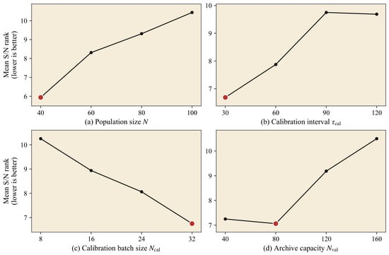
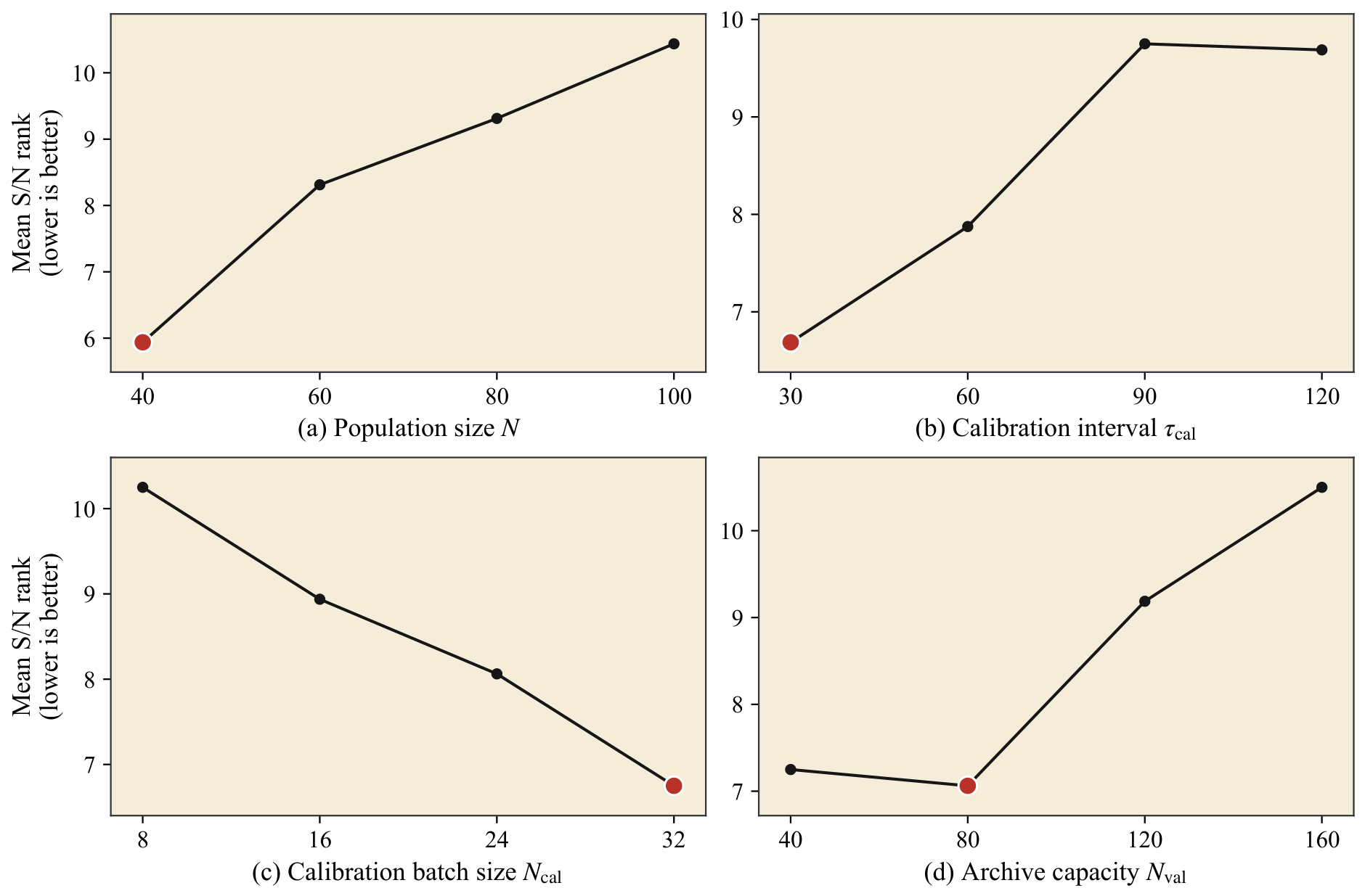
The equal-weight mean rank of the four S/N responses selects $A_1{B}_1{C}_4{D}_2$. The corresponding values are $N=40$, ${\tau }_{\mathrm{cal}}=30$, $N_{\mathrm{cal}}=32$, and $N_{\mathrm{val}}=80$. This level-effect combination is used in all subsequent experiments. Repeating the ranking with validation IGD and GD produces the same selected levels and confirms the parameter setting.

Figure 6 explains the selected levels. Under a fixed 300-s budget, increasing N worsens the mean S/N rank because fewer population updates and calibration events are completed. A shorter ${\tau }_{\mathrm{cal}}$ accelerates validation of search-archive layouts. A larger $N_{\mathrm{cal}}$ checks a broader portion of the archive at each event. The capacity effect is nonmonotonic. A capacity of 40 restricts the trade-off portfolio, while capacities above 80 retain more lower-ranked layouts. The selected levels balance search turnover, validation coverage, and decision-set size.

Figure 6. Taguchi S/N level trends of the four principal CARS-MOEA/D parameters. The ordinate is the mean rank obtained from the four S/N responses, so a lower value is better; red markers identify the selected levels $A_1{B}_1{C}_4{D}_2$.

An analysis-of-variance-style main-effect decomposition complements the level trends for the 16 S/N responses. Each factor has three degrees of freedom, and the residual of the main-effects model provides three error degrees of freedom. Table 7 reports the resulting contribution ratios. Parameter selection follows the agreement of the four S/N responses, while the main-effect p-values quantify sensitivity.

Table 7. Main-effect contribution ratios in the $L_{16}\left(4^4\right)$ parameter experiment. The unreported remainder is residual variation; the last column gives the p-value of the largest main effect.

S/N Response	A (%)	B (%)	C (%)	D (%)	Largest-Effect p
Validation HV	20.73	31.97	43.60	1.18	C: 0.022
Best validation RMSE	73.50	17.60	2.95	0.80	A: 0.028
Median validation RMSE	25.12	17.65	36.07	6.54	C: 0.239
Nondominated retention rate	3.11	4.25	8.43	83.30	D: 0.002
Mean S/N rank	36.42	31.35	24.34	3.97	A: 0.050

Note: Bold values indicate the largest main-effect contribution ratio in each row.

The composite level-range order is $A>B>C>D$. Population size has the largest effect on best validation RMSE and on the mean response rank because a larger population reduces the number of updates completed within 300 s. Calibration batch size contributes most to validation HV and median validation RMSE, showing that the number of layouts checked at each event affects both front extent and archive-wide reconstruction quality. Archive capacity dominates nondominated retention ($p=0.002$), as expected from its direct control of the returned portfolio. The agreement of the four validation responses and the unchanged choice after adding validation IGD and GD support $A_1{B}_1{C}_4{D}_2$ as a robust pre-test setting.

4.4. Comparison with Multi-Objective and Classical Placement Methods

Table 8 ranks CARS-MOEA/D first for HV, IGD, GD, best RMSE, and median RMSE under the validation-to-test route. Compared with compact calibrated MOEA/D, it improves HV by 12.64% and reduces IGD and GD by 46.70% and 47.94%. Best and median RMSE decrease by 2.76% and 8.90%. CARS-MOEA/D wins all 36 instances for the three front indicators and median RMSE, and records 35 wins and one loss for best RMSE. Friedman tests reject equal performance for all five indicators ($p\le 1.39\times {10}^{-19}$; Kendall’s $W=0.657$–$0.895$). Its paired differences from compact calibrated MOEA/D remain significant after Holm correction ($p_{\mathrm{Holm}}\le 9.61\times {10}^{-10}$), with rank-biserial correlations of 0.973–1.00.

Table 8. Average Friedman ranks of the five evolutionary algorithms over 36 instances under the validation-to-test decision route. Lower ranks are better; the best rank in each column is shown in bold.

Method	HV	IGD	GD	Best RMSE	Median RMSE
Tri-objective NSGA-II	4.861	4.472	4.694	3.833	4.333
Tri-objective MOPSO	4.000	4.417	3.722	4.444	3.611
Tri-objective MOEA/D	2.806	2.889	2.583	3.278	3.528
Compact calibrated MOEA/D	2.333	2.222	3.000	2.361	2.500
CARS-MOEA/D	1.000	1.000	1.000	1.083	1.028

Compact calibrated MOEA/D ranks first for three-dimensional HV and IGD and also obtains the best three-dimensional GD rank. CARS-MOEA/D instead ranks first for all five deployment-burden–RMSE criteria in Table 8. The two results distinguish approximation of the surrogate-objective front from selection of layouts with better held-out reconstruction performance.

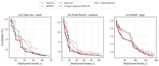
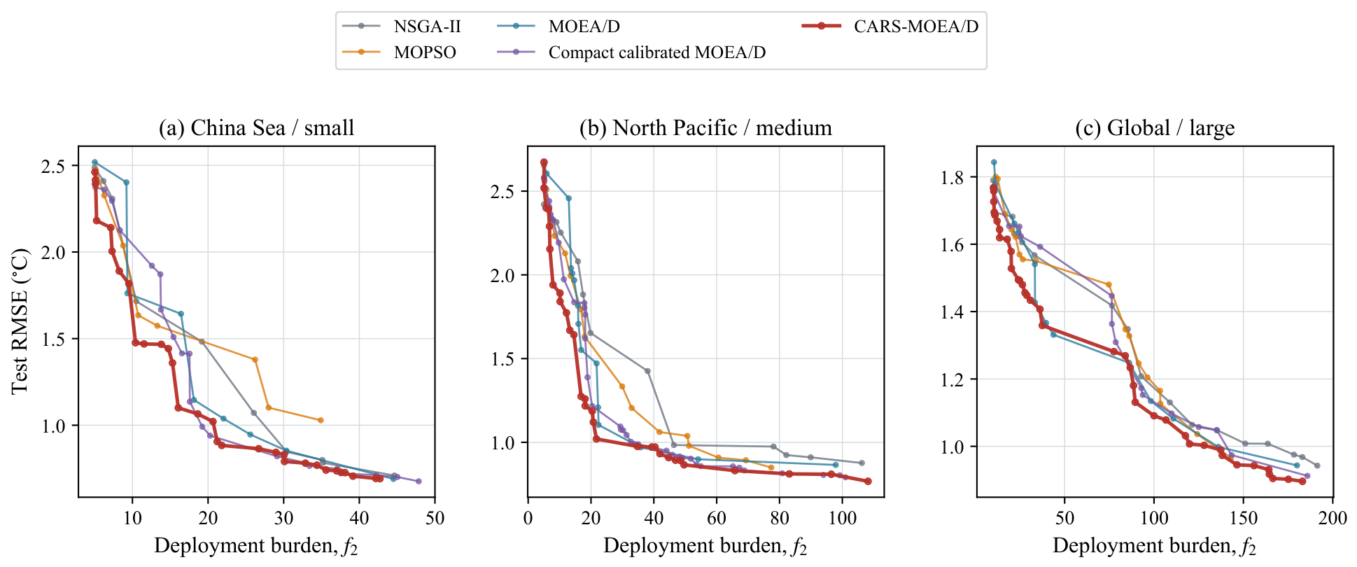
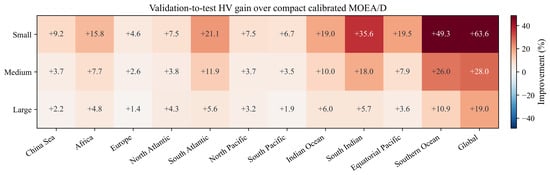
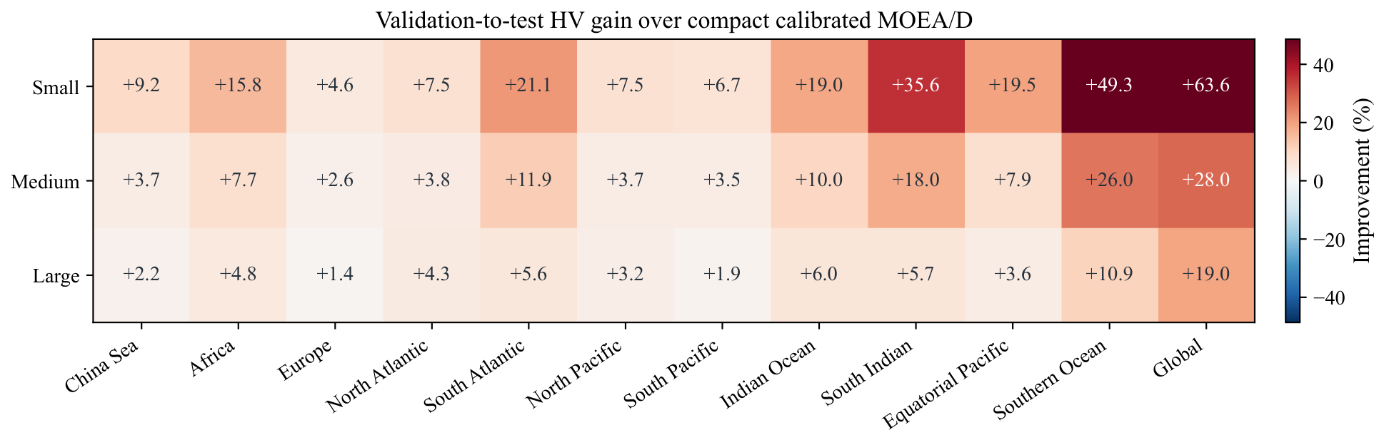
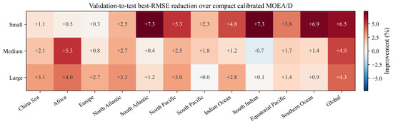
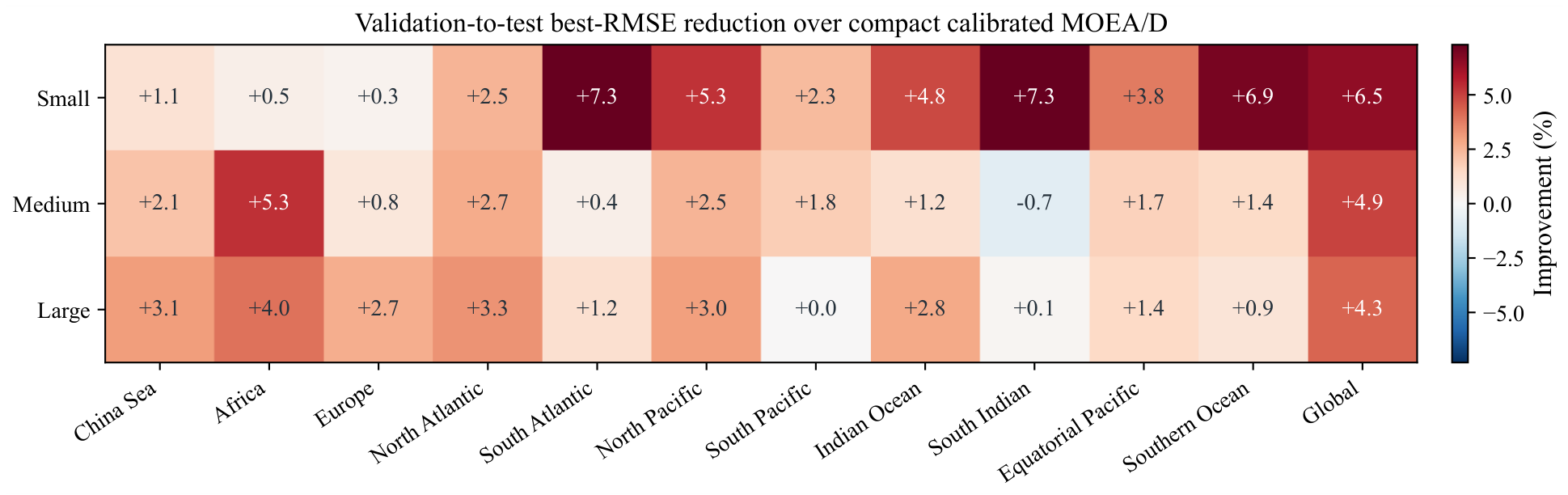
Figure 7 shows the burden–RMSE trade-offs returned for representative local, basin-scale, and global instances. The HV map in Figure 8 is positive in every region–scale cell. Mean HV gains over compact calibrated MOEA/D are 21.63%, 10.58%, and 5.71% from small to large instances, while the corresponding IGD reductions remain between 45.59% and 47.89%. Endpoint gains are less uniform: the best-RMSE map in Figure 9 contains one negative cell, although the global reductions remain 6.47%, 4.94%, and 4.27% from small to large.

Figure 7. Representative test-space nondominated subsets obtained by projecting the validation-selected layouts onto deployment burden and test RMSE for (a) the small China Sea instance, (b) the medium North Pacific instance, and (c) the large global instance. For each algorithm and instance, the run closest to its median HV over 21 repetitions is shown.

Figure 8. Validation-to-test HV improvement in CARS-MOEA/D over compact calibrated MOEA/D across twelve domains and three spatial scales. Positive values favor CARS-MOEA/D.

Figure 9. Validation-to-test reduction in best RMSE achieved by CARS-MOEA/D relative to compact calibrated MOEA/D across twelve domains and three spatial scales. Positive values favor CARS-MOEA/D.

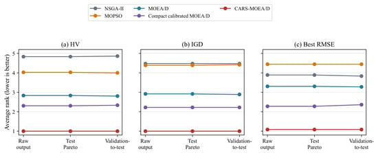
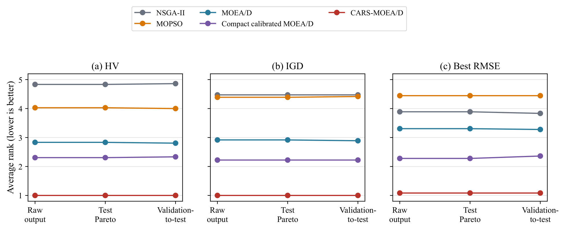
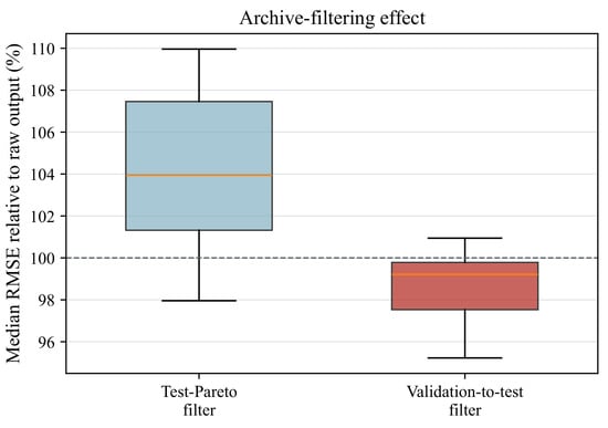
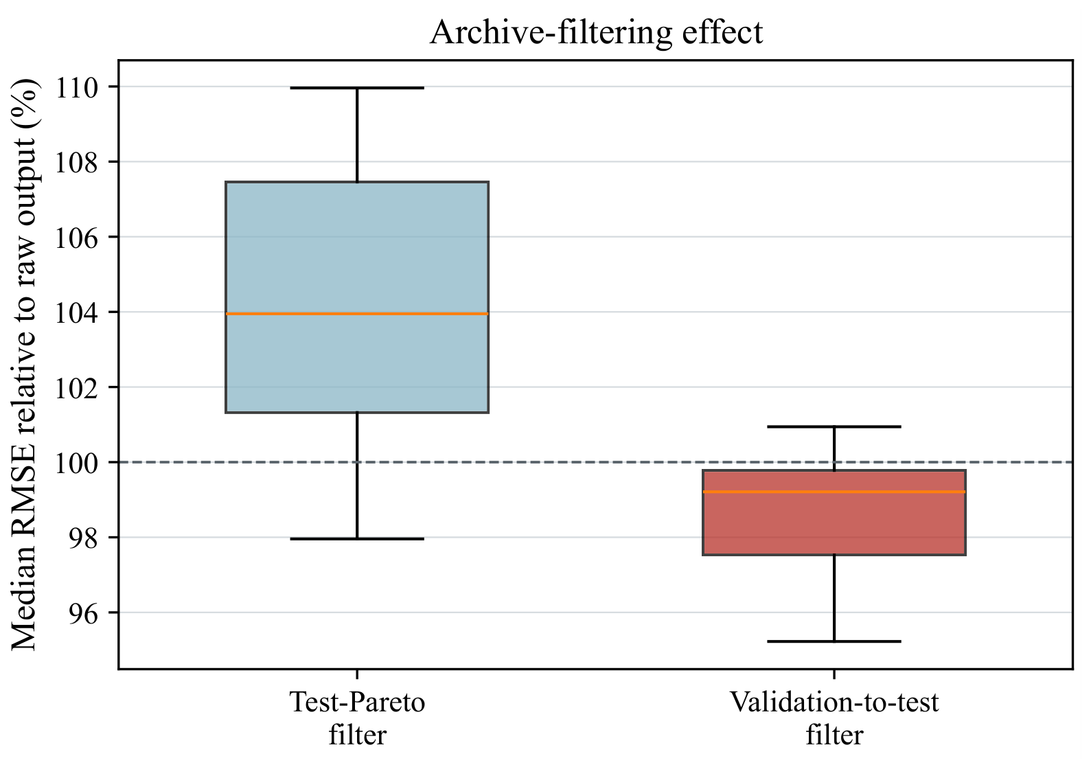
The route comparison in Figure 10 shows that CARS-MOEA/D keeps the best average rank for HV, IGD, and best RMSE under all three routes. Figure 11 shows how post-reconstruction and validation-based filtering alter the median quality of the returned set without changing the primary ranking.

Figure 10. Average algorithm ranks for HV, IGD, and best RMSE under raw-output, test-Pareto, and validation-to-test evaluation routes.

Figure 11. Effect of test-Pareto and validation-to-test archive filtering on the median RMSE of CARS-MOEA/D. Values are normalized by the corresponding raw-output median RMSE for each instance; the dashed line denotes no change.

Four classical placement strategies are additionally evaluated: K-means centers [27], leverage-score selection [11], column-pivoted QR factorization (where Q is orthogonal and R is upper triangular) with the QR-based discrete empirical interpolation method (Q-DEIM) [36], and repeated random selection. For each instance, layouts are generated at $K\in \{K_{min},max(K_{min},\lfloor r/2\rfloor ),r,2r\}$ after duplicate and infeasible values are removed. The random baseline retains the smallest-$f_1$ layout among 100 draws using seed 2026. Q-DEIM follows the full column-pivot order returned by QR and takes its first K indices, including when $K>r$. These deterministic and sampling baselines return sparse sets of layouts, so their burden–RMSE fronts are compared using HV together with bidirectional coverage. As shown in Table 9, CARS-MOEA/D achieves a larger HV on all 36 instances. Its front covers 86.4–97.6% of the baseline points on average, whereas the reverse coverage is at most 0.6%.

Table 9. Comparison with classical sensor-placement baselines over 36 instances.

Baseline	HV Wins	$\mathit{C}(\mathbf{Proposed},\mathbf{Baseline})$	$\mathit{C}(\mathbf{Baseline},\mathbf{Proposed})$
K-means centers	36/36	0.875	0.006
Leverage scores	36/36	0.864	0.000
Pivoted QR/Q-DEIM	36/36	0.968	0.001
Repeated random selection	36/36	0.976	0.001

Across the four classical strategies, the proposed front covers 86.4–97.6% of the baseline layouts, whereas reverse coverage does not exceed 0.6%. Relative to the best classical best-RMSE value on each instance, CARS-MOEA/D improves the large-scale instances by 18.74% on average and wins all 12 of them. The comparison therefore supports its advantage on the larger sparse-placement search spaces.

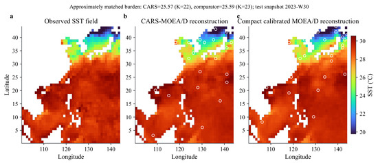
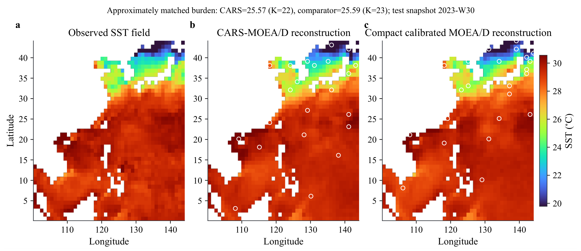
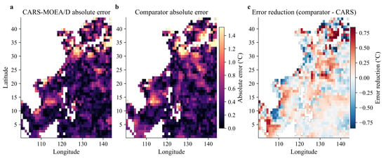
Figure 12 and Figure 13 compare the reconstructed fields and spatial errors of CARS-MOEA/D and the strongest evolutionary comparator for an approximately burden-matched medium-scale case using the same test snapshot and color scale. For each method, the run whose HV is closest to the median of 21 runs is used. The two layouts are matched without reference to test RMSE, and the displayed snapshot is the one whose instantaneous RMSE difference is closest to the median difference over the complete test period.

Figure 12. Approximately matched-burden spatial reconstruction case. (a) Observed test SST field; (b) CARS-MOEA/D reconstruction and selected layout; and (c) compact calibrated MOEA/D reconstruction and selected layout. Open circles indicate selected sensor sites. The layouts come from the median-HV runs, and the displayed snapshot represents the median instantaneous RMSE difference over the complete test period.

Figure 13. Spatial reconstruction errors for the approximately burden-matched case. (a) Absolute error of CARS-MOEA/D; (b) absolute error of the comparator; and (c) comparator error minus CARS-MOEA/D error, where positive values indicate lower error for CARS-MOEA/D. Panels (a,b) use a common color scale.

Both layouts reconstruct the broad low-latitude SST structure, with the largest errors in the northern and subtropical regions. CARS-MOEA/D reduces several coherent error patches while retaining a few localized losses. These spatial reductions produce a lower domain-wide RMSE at approximately matched burden.

4.5. Effectiveness of the Search Components

4.5.1. Contribution of the Two Proposed Components

Two variants isolate the proposed components. No-auxiliary removes $f_3$ and performs a two-objective information–burden search. No-external-refinement retains the tri-objective search but returns the information-objective archive directly. The complete method and both ablations use the same random feasible initialization, population size, variation rates, seeds, and wall-clock budgets; only the stated component is removed.

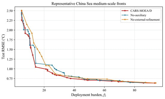
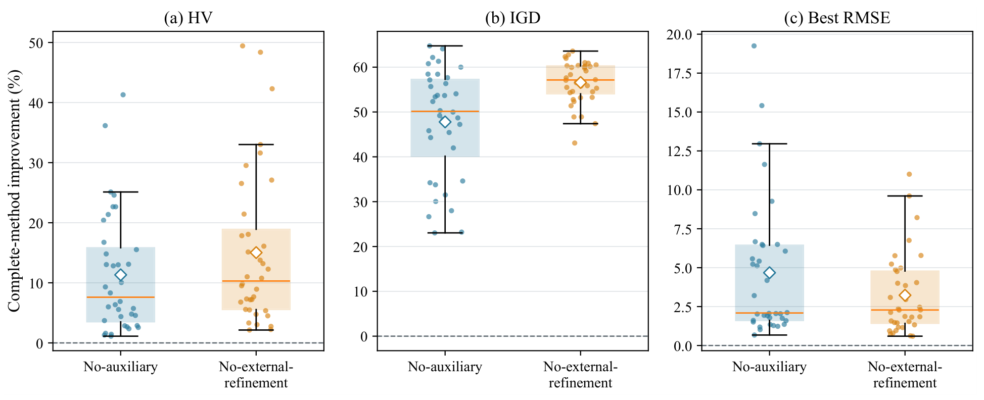
Table 10 summarizes the component effects. Relative to No-auxiliary, the complete method improves HV by 11.33% and reduces best RMSE by 4.68%, with wins on all 36 instances for HV, IGD, GD, and best RMSE. Relative to No-external-refinement, it improves HV by 15.03%, reduces GD by 49.20%, and reduces median RMSE by 11.49%. All Holm-adjusted Wilcoxon tests are significant.

Table 10. Mean improvement in CARS-MOEA/D over its ablated variants on 36 instances. Positive entries indicate an advantage of the complete method.

Removed Component	HV (%)	IGD (%)	GD (%)	BestRMSE (%)	MedianRMSE (%)
Auxiliary redundancy objective	11.33	47.79	46.10	4.68	2.98
External archive refinement module	15.03	56.58	49.20	3.23	11.49

The representative front and paired distributions in Figure 14 and Figure 15 show complementary effects. Removing the auxiliary objective increases best RMSE by 4.68%, whereas removing external refinement increases median RMSE by 11.49%. The first component improves the layouts reached during search, and the second improves the reconstruction quality of the returned archive.

Figure 14. Representative test-space nondominated subsets of the validation-selected layouts for CARS-MOEA/D, No-auxiliary, and No-external-refinement on the medium China Sea instance. For each method, the run closest to its median HV over 21 repetitions is shown.

Figure 15. Paired improvements of CARS-MOEA/D over No-auxiliary and No-external-refinement across 36 region–scale instances. Points denote instances, boxes summarize their distributions, and diamonds indicate means. Positive values favor CARS-MOEA/D.

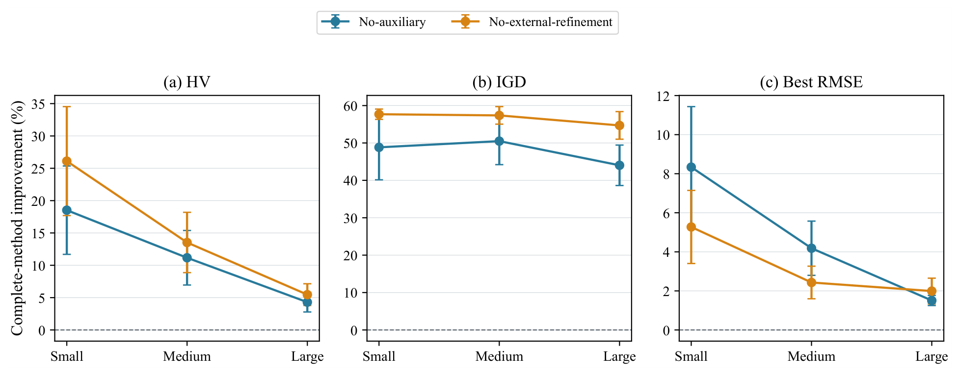
The scale-separated results in Figure 16 show that the HV and best-RMSE effects decrease with candidate-space size but remain positive at all three scales, while IGD reductions remain high across scales.

Figure 16. Scale-separated ablation effects. Markers show mean improvements over the 12 regions at each spatial scale, and error bars show 95% confidence intervals.

The two components address different failure modes. The auxiliary objective is most useful when many candidate sites have similar POD response vectors, because it redirects some decomposition subproblems toward complementary rows that the global log-determinant alone may not distinguish locally. External refinement is most useful when layouts with similar information values have different validation RMSE, because it prevents such proxy-equivalent layouts from being returned indiscriminately. Their combination is therefore expected to matter most in dense candidate grids with repeated modal patterns and under temporal transfer from the POD training period to unseen SST fields.

4.5.2. Cardinality-Controlled Role of Modal Redundancy

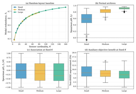
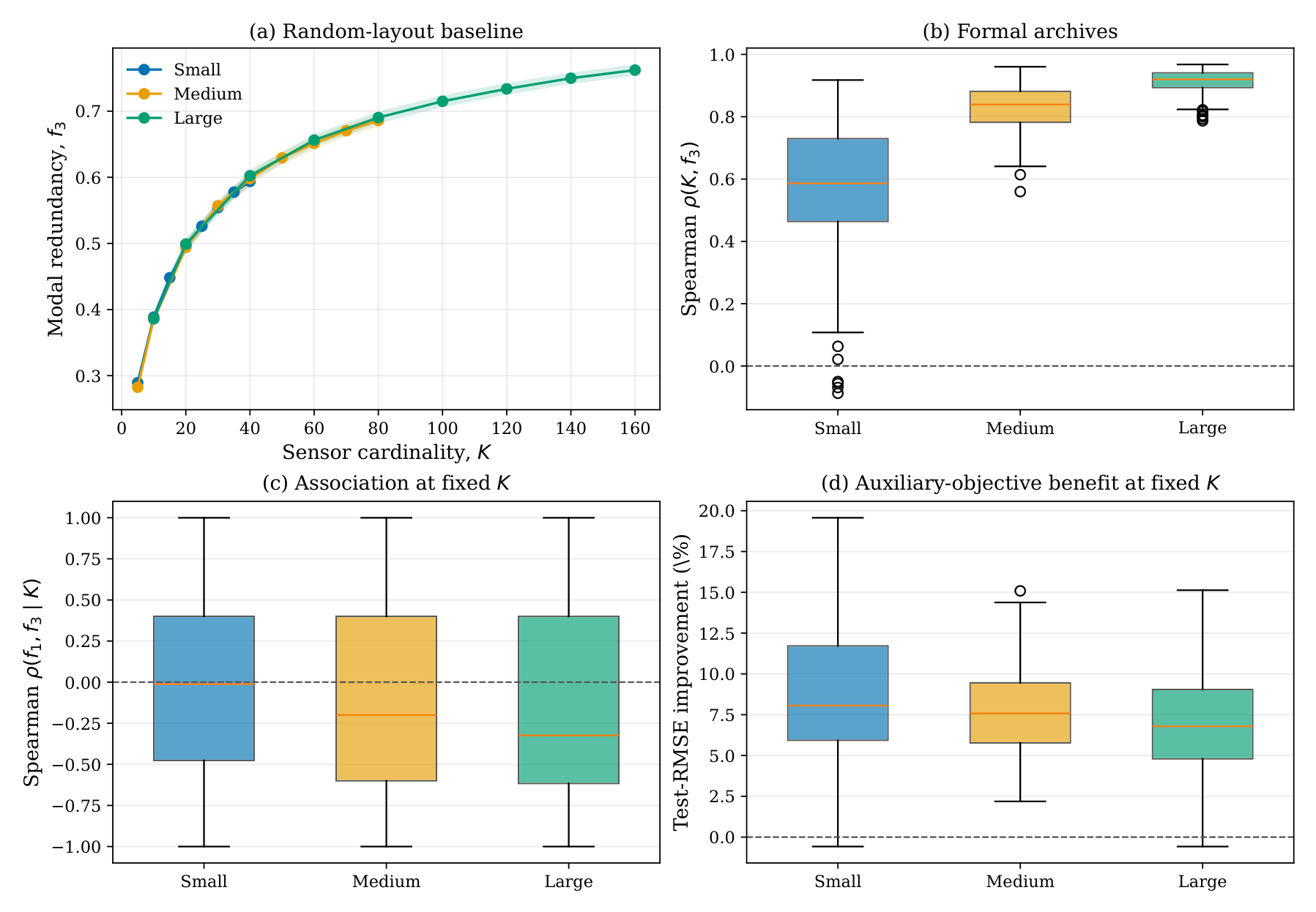
Figure 17 shows that modal redundancy increases with sensor cardinality. The pooled K–$f_3$ correlations are 0.703 for random layouts and 0.741 for 60,480 formal archive layouts; the median within-run correlation is 0.842.

Figure 17. Cardinality-sensitivity analysis of the modal-redundancy objective. (a) Mean $f_3$ of 64 random layouts per displayed K and instance; bands denote 95% confidence intervals. (b) Within-run Spearman correlations between K and $f_3$ in the 756 formal archives. (c) Spearman correlations between $f_1$ and $f_3$ within fixed-K groups. (d) Test-RMSE improvement from adding the auxiliary objective when the compared layouts have the same K; all component-isolation arms use the common initialization control.

Within fixed-K groups, the median $f_1$–$f_3$ correlation is $-0.179$, and the partial-rank median is $-0.124$. At the same K, the auxiliary-objective arm reduces test RMSE by 7.86%, improves 753 of 756 runs, and yields positive mean gains on all 36 instances. Because each comparison uses an identical sensor cardinality, the gain cannot be attributed to selecting more sensors. Together with the normalized simplex decomposition in Equation (18), this result shows that $f_3$ introduces complementary search directions without displacing the information-oriented subproblems, including comparisons drawn from the lower part of each admissible sensor range.

4.5.3. Auxiliary Objective Versus Fixed-Threshold Control

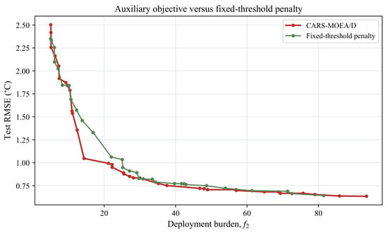
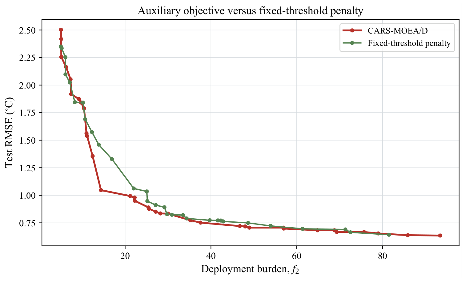
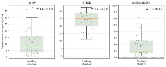
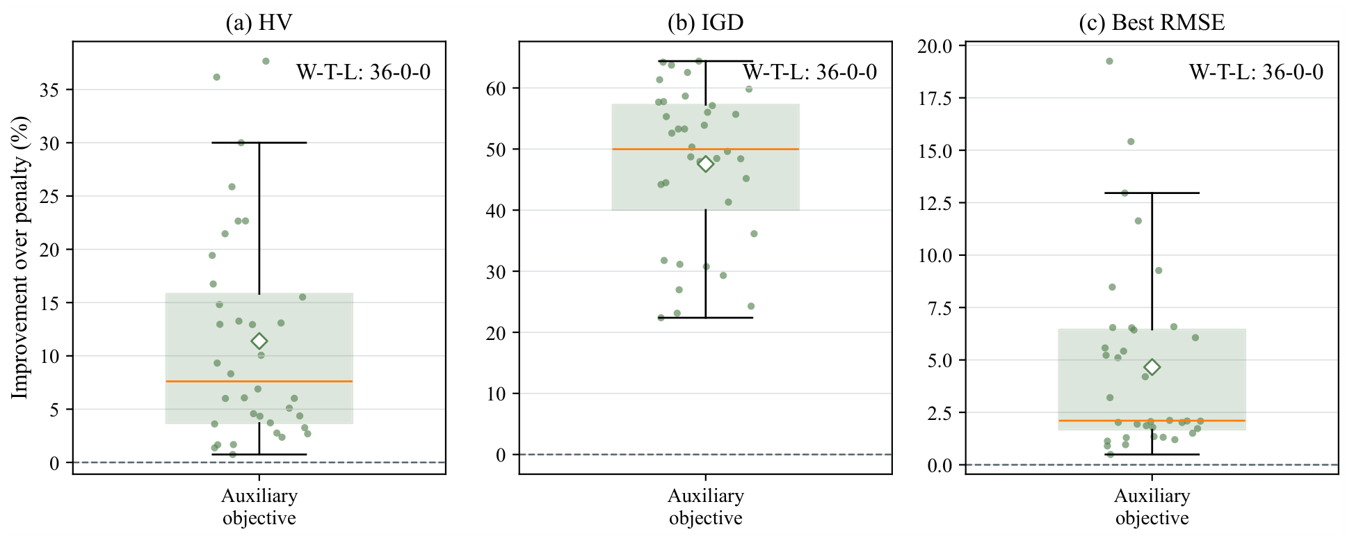
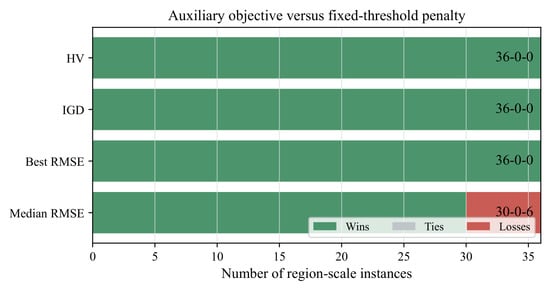
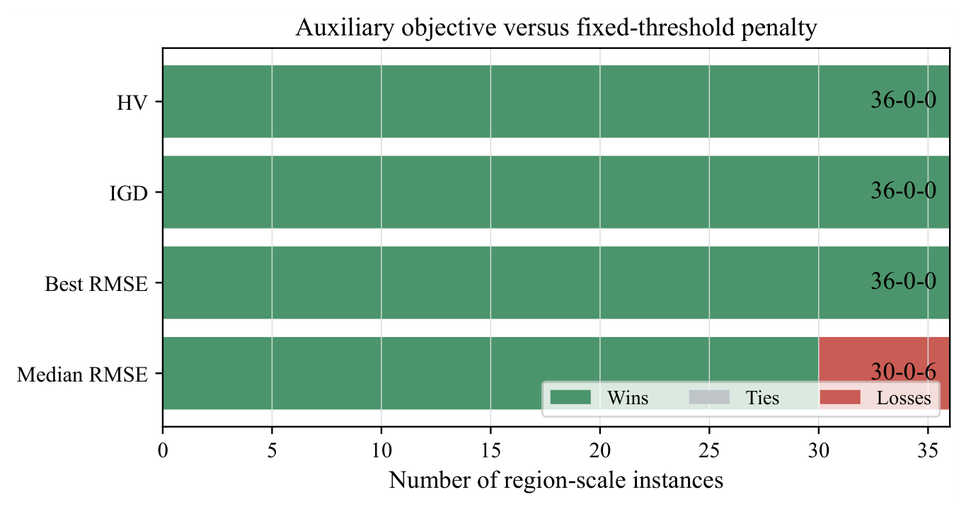
To determine how modal redundancy should guide search, CARS-MOEA/D is compared with a penalty-enforced redundancy control. Both methods use the same budgets and component-isolation initialization. The control defines $v\left(X\right)=max\{0,f_3\left(X\right)-0.75\}$ and optimizes $f_1\left(X\right)+25v\left(X\right)$ together with $f_2\left(X\right)$. The auxiliary-objective formulation improves HV by 11.39%, reduces IGD and GD by 47.55% and 46.96%, and reduces best RMSE by 4.66%. It wins all 36 instances on these four indicators. Median RMSE improves by 2.90%, with 30 wins and 6 losses. The representative fronts in Figure 18, paired improvements in Figure 19, and win–tie–loss counts in Figure 20 show that the auxiliary objective provides a more effective search direction than the fixed-threshold penalty.

Figure 18. Representative test-space nondominated subsets of the validation-selected layouts obtained by treating modal redundancy as an auxiliary objective or as a fixed-threshold penalty control on the medium China Sea instance. For each method, the run closest to its median HV over 21 repetitions is shown.

Figure 19. Paired performance improvements in CARS-MOEA/D over the fixed-threshold penalty control across 36 instances. Positive values favor CARS-MOEA/D.

Figure 20. Win–tie–loss counts of CARS-MOEA/D against the fixed-threshold penalty control.

4.6. Time-Aware Performance, Robustness, and Sensitivity

4.6.1. Anytime Search Behavior

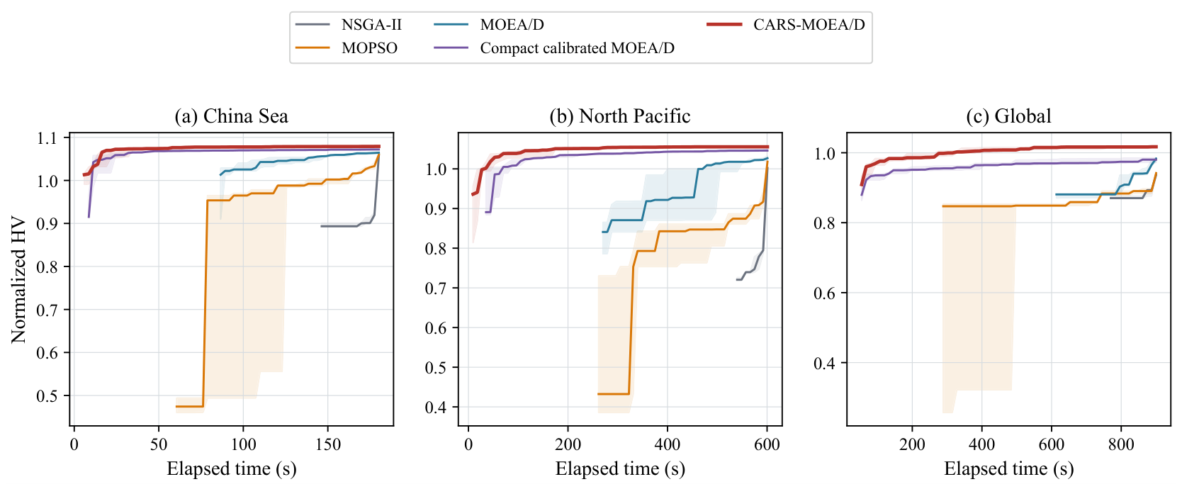
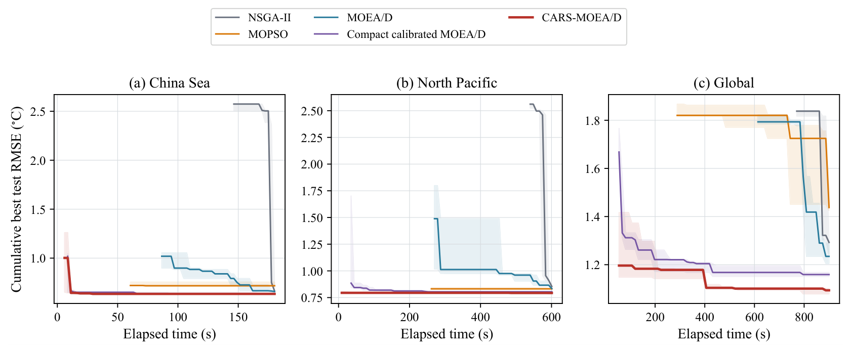
The anytime experiment records when retained layouts are discovered on the medium China Sea, North Pacific, and global instances. At each time point, accumulated layouts determine normalized burden–test-RMSE HV and cumulative best test RMSE. Each method is repeated five times; lines and bands report the median and interquartile range after all runs return a layout.

Figure 21 and Figure 22 show that CARS-MOEA/D reaches a high-quality front early and continues to improve it throughout the budget. At the common stopping times, it obtains the best median endpoint HV and best RMSE on all three instances. Relative to the strongest endpoint competitor in each case, its mean gains are 1.66% in HV and 2.50% in best RMSE, with the largest best-RMSE gain occurring on the global instance.

Figure 21. Time-aware normalized HV of the tested layouts discovered by the five evolutionary algorithms on representative local, basin-scale, and global medium instances. Lines and shaded bands denote medians and interquartile ranges over five runs.

Figure 22. Cumulative best test RMSE of the layouts discovered under the same equal-time protocol. Lower values are better.

4.6.2. Empirical Runtime Growth

The asymptotic costs in Section 3 were complemented by single-process, single-thread timings. Table 11 separates one joint $f_1$–$f_3$ evaluation from one validation reconstruction over all 159 validation snapshots. At fixed $K=20$, the objective time remains below 0.08 ms from the 339-site local instance to the 172,681-site global instance, whereas validation reconstruction increases from 0.515 to 314.565 ms because it operates on the full field. On the global instance, increasing K from 5 to 160 raises the joint objective time from 0.069 to 0.207 ms, consistent with the K-dependent terms in the complexity analysis. These measurements explain why the inexpensive objectives are used throughout the search and full-field RMSE is evaluated only for a bounded calibration batch.

Table 11. Single-thread empirical cost of one joint objective evaluation and one validation reconstruction.

Case	P	r	K	${\mathit{f}}_1$–${\mathit{f}}_3$ (ms)	Validation (ms)
China Sea, small	339	20	20	0.050	0.515
China Sea, medium	1283	20	20	0.050	1.621
China Sea, large	5169	20	20	0.050	6.512
Global, large	172,681	50	20	0.071	314.565
Global, large	172,681	50	5	0.069	313.904
Global, large	172,681	50	80	0.112	313.125
Global, large	172,681	50	160	0.207	313.211

4.6.3. Deployment-Burden Sensitivity

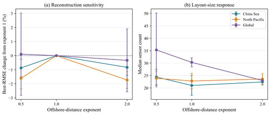
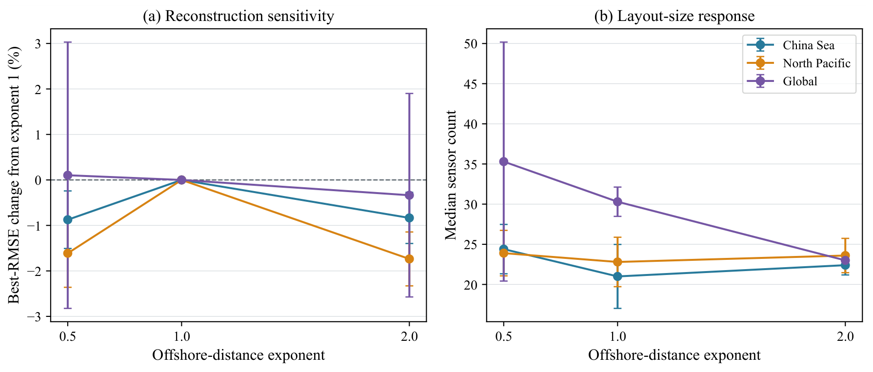
Sensitivity to offshore-distance scaling is evaluated at $\gamma \in \{0.5,1,2\}$ on the same representative regions, with all other settings fixed.

As shown in Figure 23a, the mean best-RMSE change remains between $-1.74\%$ and 0.04%. Reconstruction quality is therefore stable across the tested exponents. Figure 23b shows a clearer layout-size response, especially for the global case, where the median sensor count decreases from 35.3 to 23.0 as $\gamma$ increases from 0.5 to 2. The exponent mainly changes the preferred burden allocation rather than the attainable reconstruction accuracy.

Figure 23. Sensitivity to the offshore-distance exponent: changes in best RMSE relative to exponent 1 and the corresponding median sensor counts. Markers and error bars show means and 95% confidence intervals over five runs.

This sensitivity test quantifies the effect of the offshore-distance scaling used in the present burden proxy. The proxy does not represent monetary cost and does not yet include bathymetry, vessel route and home port, sea-state exposure, communication demand, or station-specific failure history. Those factors may change the preferred layout even when the information objective is unchanged; their incorporation requires consistent engineering data and application-specific weights.

4.6.4. POD-Rank Sensitivity on the Large Global Instance

The retained-rank upper bound is examined on the most demanding 172,681-site global instance using $r\in \{50,75,100\}$. Each rank is independently repeated 21 times under the same 2400-s budget. Table 12 shows that increasing r captures more training variance and lowers the POD truncation error, but it does not improve sparse reconstruction under the tested sensor-number range. Relative to $r=50$, the mean best test RMSE increases by 9.74% at $r=75$ and by 26.80% at $r=100$. The nondominated retention rate remains between 0.454 and 0.480. Thus, the $r=50$ cap does not limit the best reconstruction obtained in this global experiment; higher-dimensional coefficient estimation instead becomes less favorable for the available sparse observations and fixed search budget.

Table 12. POD-rank sensitivity on the large global instance (mean over 21 runs).

r	Variance	Test Truncation RMSE	Best Test RMSE	${\mathit{R}}_{\mathbf{ND}}$	Normalized HV
50	0.9501	0.7001	0.8839	0.463	0.8065
75	0.9612	0.6824	0.9700	0.480	0.6603
100	0.9683	0.6670	1.1207	0.454	0.5411

4.6.5. Observation Noise and Sensor Dropout

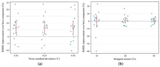
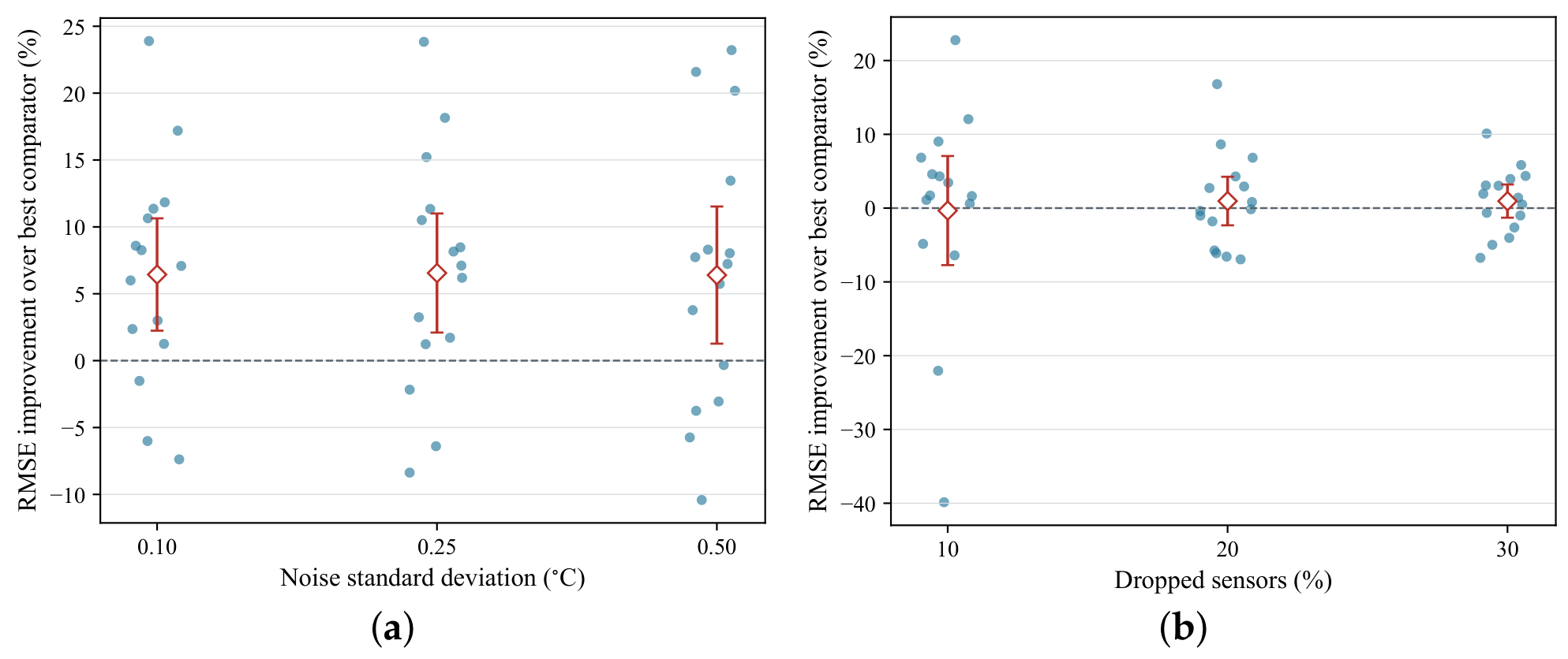
Observation-noise robustness is first examined on the same three medium-scale regions using five seeds and all 212 test snapshots. Gaussian measurement noise with standard deviations of 0.1, 0.25, and 0.5 °C is independently generated ten times for each layout. For the dropout test, each region–seed block uses the sensor cardinality shared by all five algorithms that is nearest $K=20$; the resulting matched cardinalities range from 14 to 22. At 10%, 20%, and 30% dropout, all algorithms in a block receive the same 30 randomly generated retained-position patterns, and reconstruction is evaluated on every fourth test snapshot. In each setting, CARS-MOEA/D is compared with the strongest scenario-specific method for that region–seed block.

Figure 24 shows mean RMSE advantages of 6.44%, 6.55%, and 6.40% at noise standard deviations of 0.1, 0.25, and 0.5 °C. CARS-MOEA/D wins 12, 12, and 10 of the 15 region–seed blocks, respectively.

Figure 24. Reconstruction robustness under observational perturbations. (a) RMSE improvement in CARS-MOEA/D over the strongest scenario-specific comparator under Gaussian observation noise; blue points denote the 15 region–seed blocks, and red diamonds and error bars show means and 95% confidence intervals. (b) RMSE improvement under matched-cardinality, strictly paired sensor dropout; negative values indicate cases in which CARS-MOEA/D does not retain an RMSE advantage.

Under strictly paired sensor dropout, the mean (median) RMSE advantages are $-0.33\%$ (1.71%), 0.96% ($-0.15\%$), and 0.95% (1.41%) at 10%, 20%, and 30%, with 11, 7, and 9 wins among the 15 region–seed blocks, respectively. The confidence intervals include zero at all three dropout levels, indicating comparable aggregate robustness rather than a uniform advantage. The larger spread at 10% dropout further shows that the effect of losing a small number of sites depends on which locations are removed from each layout.

4.7. Operational Validation on the TAO Buoy Network

4.7.1. Data and Observation Calibration

To examine whether layouts learned from a gridded product transfer to an operational in situ network, an additional case study uses the TAO moored-buoy array in the tropical Pacific [7,9]. The engineering question is a constrained retention problem: if only K stations can be operated or prioritized, which stations should remain primary, which stations are most critical, and which unselected stations should be designated as backups? The downloaded archive contains 775 deployment files associated with 58 historical station records. For each deployment file, the shallowest available SST channel is used; observations outside the physical SST range or with TAO quality flags other than 1, 2, or 5 are discarded before duplicate-date resolution. Applying a training-period availability threshold of 30% then leaves 55 eligible candidate sites. Each site is mapped by great-circle distance to its nearest valid $1^{\circ }$ OISST ocean cell; the maximum separation is 19.7 km and no two stations map to the same cell. The dense 3874-cell OISST domain remains the source of the POD basis and full-field reference, whereas TAO supplies realizable station coordinates and recorded in situ SST observations. Thus, the case represents offline field-model learning followed by network thinning and operation at existing observation sites.

Four sensor budgets, $K\in \{5,10,15,20\}$, are tested. Tri-objective NSGA-II, tri-objective MOPSO, tri-objective MOEA/D, and CARS-MOEA/D are independently run 21 times; compact calibrated MOEA/D is excluded because the TAO case focuses on the proposed method, its unrefined decomposition baseline, and algorithms based on distinct evolutionary paradigms. K-means, leverage-score selection, pivoted QR/Q-DEIM, and repeated random selection are included as classical baselines. The temporal split remains unchanged: 2010–2018 for POD learning and observation calibration, 2019–2021 for layout selection, and 2022–2025 for temporally held-out testing. Two evaluation routes are distinguished. The ideal route samples OISST at the TAO coordinates and isolates placement quality from instrument effects. The operational route uses the recorded TAO observations and their historical missing pattern. In addition to raw observations and median-bias correction, a station-wise affine transfer

$$y_{i,t}^{\mathrm{OISST}}={\alpha }_i+{\beta }_i{y}_{i,t}^{\mathrm{TAO}}+e_{i,t}$$

(23)

is fitted using paired training observations only. At test time, the active station subset $X_t$ is used in the weighted ridge system

$${\widehat{\mathit{a}}}_t={\left({\mathrm{\Phi }}_{X_t}^{\top }{W}_t{\mathrm{\Phi }}_{X_t}+\rho I\right)}^{-1}{\mathrm{\Phi }}_{X_t}^{\top }{W}_t\left({\tilde{\mathit{y}}}_{X_t,t}-{\overline{\mathit{x}}}_{X_t}\right),$$

(24)

where ${\tilde{\mathit{y}}}_{X_t,t}$ contains the affine-transferred observations, and ${\widehat{\sigma }}_{e,i}$ is the training-period standard deviation of residual $e_{i,t}$. The diagonal weights in $W_t$ are proportional to $1/max{({\widehat{\sigma }}_{e,i},0.05)}^2$ and normalized by their median. The median station-wise $R^2$ is 0.937, and the median residual standard deviation is 0.254 °C, indicating that the fitted transfer is sufficiently stable for held-out evaluation.

4.7.2. Candidate-Availability Threshold Sensitivity

The training-period availability threshold and the residual weights act at different stages. The threshold is applied before optimization and controls whether a historical station is eligible for the candidate set. Equation (24) is applied after a layout is selected and controls the contribution of stations that are active at a given test time according to their training residual variance. A stricter eligibility threshold therefore cannot replace residual weighting: the former changes the spatial choice set, whereas the latter changes the reliability of simultaneous observations during reconstruction.

Thresholds of 0.30, 0.50, 0.60, and 0.70 are evaluated for $K\in \{5,10,15,20\}$, with 21 independent runs per setting. Table 13 reports averages over the four sensor budgets. Raising the threshold from 0.30 to 0.50 removes only two candidate sites and produces nearly unchanged full-field RMSE. Thresholds of 0.60 and 0.70 reduce the candidate set to 45 and 27 sites and increase the affine-weighted full-field RMSE from 1.0590 to 1.0735 and 1.0669 °C, respectively. The 0.30 threshold is therefore retained because it preserves the broadest spatial choice set, while the weighted reconstruction still accounts for station-specific observation quality.

Table 13. Sensitivity to the training-period TAO availability threshold. RMSE and operational quantities are averaged over $K=5,10,15,20$ and 21 runs per budget.

Threshold	Candidate Sites	Ideal Full-Field RMSE	Weighted Full-Field RMSE	Held-out-Station RMSE	Selected-Site Availability	Reconstruction Coverage
0.30	55	0.9327	1.0590	0.8447	0.317	0.912
0.50	53	0.9331	1.0590	0.8344	0.336	0.906
0.60	45	0.9376	1.0735	0.9045	0.323	0.971
0.70	27	0.9326	1.0669	0.8666	0.339	0.982

4.7.3. Station-Retention Performance

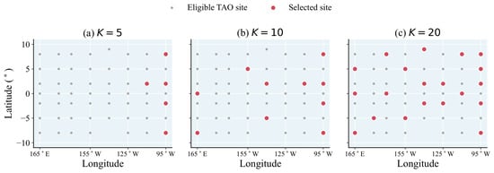
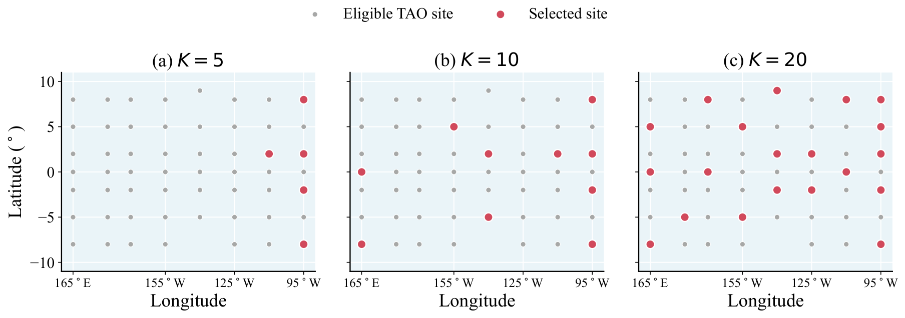
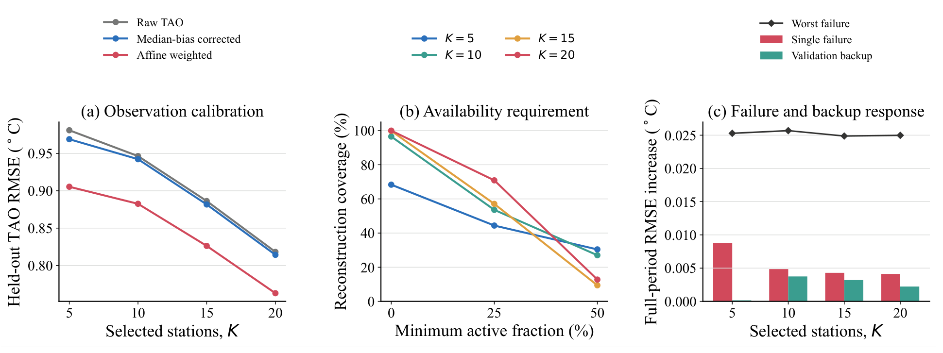
Figure 25 shows the eligible network and representative CARS-MOEA/D layouts selected by median validation RMSE. Under ideal OISST sampling, CARS-MOEA/D has the lowest mean full-field RMSE among the evolutionary algorithms for every sensor budget and improves on the strongest competitor by 1.09–2.24%. Under recorded TAO sampling, affine residual weighting lowers held-out-station RMSE by 0.051–0.064 °C relative to median-bias correction. CARS-MOEA/D obtains the best average held-out-station rank (1.50) among the four evolutionary methods and ranks second for full-field RMSE behind MOPSO. The operational case therefore establishes its strength in unobserved-station prediction and competitive full-field transfer.

Figure 25. TAO engineering case. Gray markers are the 55 eligible historical TAO sites, and red markers are representative CARS-MOEA/D layouts for three illustrative sensor budgets ($K=5$, 10, and 20); all four budgets, including $K=15$, are evaluated in the quantitative analysis. Each stochastic layout is the median validation-RMSE run among 21 independent runs.

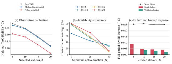
Operational network utility also depends on how often enough selected stations are active. With at least one active station required, reconstruction coverage of CARS-MOEA/D increases from 68.4% at $K=5$ to 96.5%, 99.8%, and 100% at $K=10$, 15, and 20, respectively. Requiring at least half of the selected stations reduces conditional RMSE but decreases coverage to 30.4%, 27.0%, 9.4%, and 12.8%. Figure 26b reports the corresponding coverage, while the accompanying conditional calculations provide the RMSE values stated above. Joint reporting of accuracy and coverage distinguishes reliable operation from low errors computed on a small subset of well-observed dates.

Figure 26. Operational assessment of the TAO layouts. (a) Held-out-station RMSE under raw, median-bias-corrected, and affine-weighted TAO inputs; (b) reconstruction coverage under different minimum active-station requirements; and (c) mean and worst single-station failure penalties together with validation-selected backup-site penalties.

4.7.4. Failure and Backup Analysis

After layout generation, reliability is evaluated by permanently removing each selected station in turn from a representative layout chosen on validation data. The mean full-period RMSE increases are 0.0088, 0.0049, 0.0043, and 0.0041 °C for $K=5$, 10, 15, and 20, while the worst increase remains below 0.0257 °C. Station T2S95W is the most critical site at all four budgets. For each failed station, one unselected backup is then chosen by validation-period reconstruction error, with information and burden used as tiebreakers. This post hoc strategy reduces the mean failure penalty by 98.3%, 22.8%, 25.6%, and 46.0%, respectively. The analysis therefore supports station-retention, maintenance-priority, and contingency decisions after layout selection.

Beyond TAO, the workflow can be transferred after rebuilding the POD basis, candidate mask, and site-burden vector from the target data. Transfer is direct when the field is adequately represented by a low-dimensional basis, and candidate observations can be mapped to that basis; strongly nonstationary coastal dynamics, moving platforms, or system-specific operational constraints require retraining and a revised burden formulation.

5. Conclusions

This study proposes CARS-MOEA/D for cost-aware SST sensor placement. Redundancy-assisted decomposition search generates complementary layouts, while validation-calibrated archiving retains reconstruction–burden trade-offs. Across 36 OISST instances, CARS-MOEA/D obtains the best overall ranks among the tested evolutionary algorithms on the validation-to-test reconstruction–burden criteria. Ablation and fixed-cardinality results confirm the contributions of the auxiliary redundancy objective and archive refinement. The fixed-cardinality evidence further shows that the redundancy direction improves reconstruction without relying on a larger sensor budget, while the global-rank and TAO-threshold analyses delimit the effects of POD dimension and candidate-site eligibility.

The TAO case further demonstrates the operational applicability of the framework under historical missingness and station failures. The present burden objective remains a reproducible within-domain proxy rather than a complete engineering cost model, and the method assumes that a fixed POD basis adequately represents the deployment period. Future work will incorporate operational-access and reliability factors, adaptive basis updates, and network-specific constraints, and will examine transfer to coastal arrays and observation systems for other ocean variables.

References

- Huang, B.; Liu, C.; Banzon, V.; Freeman, E.; Graham, G.; Hankins, B.; Smith, T.M.; Zhang, H.M. Improvements of the daily optimum interpolation sea surface temperature (DOISST) version 2.1. J. Clim. 2021, 34, 2923–2939. [Google Scholar] [CrossRef] [Scilit]
- St. Amand, F.M.; Maasch, K.A.; Sandweiss, D.H. Assessing the accuracy of MUR high resolution satellite sea surface temperature data. Remote Sens. Appl. Soc. Environ. 2024, 36, 101267. [Google Scholar] [CrossRef] [Scilit]
- Benzouai, S.; Dries, R.; Benkhelifa, S.; Louanchi, F.; Smara, Y. Spatio-temporal variability of sea surface temperature in the Algerian Sea (SW Mediterranean Sea), from 37 years of analyzed data. Reg. Stud. Mar. Sci. 2024, 74, 103511. [Google Scholar] [CrossRef] [Scilit]
- Cheng, L.; Abraham, J.; Trenberth, K.E.; Fasullo, J.; Boyer, T.; Mann, M.E.; Zhu, J.; Wang, F.; Locarnini, R.; Li, Y.; et al. Another year of record heat for the oceans. Adv. Atmos. Sci. 2023, 40, 963–974. [Google Scholar] [CrossRef] [Scilit] [PubMed]
- Smith, K.E.; Burrows, M.T.; Hobday, A.J.; King, N.G.; Moore, P.J.; Sen Gupta, A.; Thomsen, M.S.; Wernberg, T.; Smale, D.A. Biological impacts of marine heatwaves. Annu. Rev. Mar. Sci. 2023, 15, 119–145. [Google Scholar] [CrossRef] [Scilit] [PubMed]
- Goh, E.; Yepremyan, A.; Wang, J.; Wilson, B. MAESSTRO: Masked autoencoders for sea surface temperature reconstruction under occlusion. Ocean Sci. 2024, 20, 1309–1323. [Google Scholar] [CrossRef] [Scilit]
- McPhaden, M.J.; Busalacchi, A.J.; Cheney, R.; Donguy, J.R.; Gage, K.S.; Halpern, D.; Ji, M.; Julian, P.; Meyers, G.; Mitchum, G.T.; et al. The Tropical Ocean-Global Atmosphere observing system: A decade of progress. J. Geophys. Res. Ocean. 1998, 103, 14169–14240. [Google Scholar] [CrossRef] [Scilit]
- Fujii, Y.; Rémy, E.; Zuo, H.; Oke, P.; Halliwell, G.; Gasparin, F.; Benkiran, M.; Loose, N.; Cummings, J.; Xie, J.; et al. Observing system evaluation based on ocean data assimilation and prediction systems: On-going challenges and a future vision for designing and supporting ocean observational networks. Front. Mar. Sci. 2019, 6, 417. [Google Scholar] [CrossRef] [Scilit]
- Smith, N.; Kessler, W.S.; Cravatte, S.; Sprintall, J.; Wijffels, S.; Cronin, M.F.; Sutton, A.; Serra, Y.L.; Dewitte, B.; Strutton, P.G.; et al. Tropical Pacific Observing System. Front. Mar. Sci. 2019, 6, 31. [Google Scholar] [CrossRef] [Scilit]
- Everson, R.; Sirovich, L. Karhunen–Loève procedure for gappy data. J. Opt. Soc. Am. A 1995, 12, 1657–1664. [Google Scholar] [CrossRef] [Scilit]
- Manohar, K.; Brunton, B.W.; Kutz, J.N.; Brunton, S.L. Data-driven sparse sensor placement for reconstruction: Demonstrating the benefits of exploiting known patterns. IEEE Control Syst. Mag. 2018, 38, 63–86. [Google Scholar] [CrossRef] [Scilit]
- Juhlin, M.; Jakobsson, A. Optimal sensor placement for localizing structured signal sources. Signal Process. 2023, 202, 108679. [Google Scholar] [CrossRef] [Scilit]
- Kim, S.H.; Cho, C. Effective independence in optimal sensor placement associated with general Fisher information involving full error covariance matrix. Mech. Syst. Signal Process. 2024, 212, 111263. [Google Scholar] [CrossRef] [Scilit]
- Zhang, Z.; Gao, X.; Chen, Q.; Yuan, Y. A novel thermal turbulence reconstruction method using proper orthogonal decomposition and compressed sensing coupled based on improved particle swarm optimization for sensor arrangement. Phys. Fluids 2024, 36, 055124. [Google Scholar] [CrossRef] [Scilit]
- Hosseini, M.Y.; Shiri, Y. Flow field reconstruction from sparse sensor measurements with physics-informed neural networks. Phys. Fluids 2024, 36, 073606. [Google Scholar] [CrossRef] [Scilit]
- Zou, J.; Qiu, W.; Sun, Z.; Zhang, X.; Zhang, Z.; Zhu, X.; Liang, D.; Chen, W.; Yan, C. Joint optimization of sensor placement and sparse pressure field reconstruction with a two-stage framework for limited data. Phys. Fluids 2025, 37, 075231. [Google Scholar] [CrossRef] [Scilit]
- Liang, A.; Xu, D.; Chen, D.; Cui, W.; Liu, Q. Online sparse sensor placement with mobility constraints for pollution plume reconstruction. J. Mar. Sci. Eng. 2025, 13, 1995. [Google Scholar] [CrossRef] [Scilit]
- Zhang, Y.; Bellingham, J.G. An efficient method of selecting ocean observing locations for capturing the leading modes and reconstructing the full field. J. Geophys. Res. Ocean. 2008, 113, C04005. [Google Scholar] [CrossRef] [Scilit]
- Yang, X.; Venturi, D.; Chen, C.; Chryssostomidis, C.; Karniadakis, G.E. EOF-based constrained sensor placement and field reconstruction from noisy ocean measurements: Application to Nantucket Sound. J. Geophys. Res. Ocean. 2010, 115, C12072. [Google Scholar] [CrossRef] [Scilit]
- Li, Z.; Du, Q.; Qian, B.; Hu, R.; Xu, M. Dual learning based Pareto evolutionary algorithm for a kind of multi-objective task assignment problem. Expert Syst. Appl. 2025, 276, 127006. [Google Scholar] [CrossRef] [Scilit]
- Li, Z.; Xing, Q.; Hu, R.; Qian, B. Pareto evolutionary algorithm based on Markov chain for portfolio optimization considering profit of assets. Expert Syst. Appl. 2026, 296, 129144. [Google Scholar] [CrossRef] [Scilit]
- Zhang, Q.; Li, H. MOEA/D: A multiobjective evolutionary algorithm based on decomposition. IEEE Trans. Evol. Comput. 2007, 11, 712–731. [Google Scholar] [CrossRef] [Scilit]
- Zheng, W.; Tan, Y.; Yan, Z.; Yang, M. A novel clustering-based evolutionary algorithm with objective space decomposition for multi/many-objective optimization. Inf. Sci. 2024, 677, 120940. [Google Scholar] [CrossRef] [Scilit]
- Nakai, K.; Yamada, K.; Nagata, T.; Saito, Y.; Nonomura, T. Effect of objective function on data-driven greedy sparse sensor optimization. IEEE Access 2021, 9, 46731–46743. [Google Scholar] [CrossRef] [Scilit]
- Saito, Y.; Nonomura, T.; Yamada, K.; Nakai, K.; Nagata, T.; Asai, K.; Sasaki, Y.; Tsubakino, D. Determinant-based fast greedy sensor selection algorithm. IEEE Access 2021, 9, 68535–68551. [Google Scholar] [CrossRef] [Scilit]
- Joshi, S.; Boyd, S. Sensor selection via convex optimization. IEEE Trans. Signal Process. 2009, 57, 451–462. [Google Scholar] [CrossRef] [Scilit]
- Lloyd, S.P. Least squares quantization in PCM. IEEE Trans. Inf. Theory 1982, 28, 129–137. [Google Scholar] [CrossRef] [Scilit]
- Deb, K.; Pratap, A.; Agarwal, S.; Meyarivan, T. A fast and elitist multiobjective genetic algorithm: NSGA-II. IEEE Trans. Evol. Comput. 2002, 6, 182–197. [Google Scholar] [CrossRef] [Scilit]
- Coello Coello, C.A.; Pulido, G.T.; Lechuga, M.S. Handling multiple objectives with particle swarm optimization. IEEE Trans. Evol. Comput. 2004, 8, 256–279. [Google Scholar] [CrossRef] [Scilit]
- Zitzler, E.; Thiele, L.; Laumanns, M.; Fonseca, C.M.; da Fonseca, V.G. Performance assessment of multiobjective optimizers: An analysis and review. IEEE Trans. Evol. Comput. 2003, 7, 117–132. [Google Scholar] [CrossRef] [Scilit]
- Ishibuchi, H.; Masuda, H.; Tanigaki, Y.; Nojima, Y. Modified distance calculation in generational distance and inverted generational distance. In Proceedings of the 8th International Conference on Evolutionary Multi-Criterion Optimization (EMO 2015), Guimarães, Portugal, 29 March–1 April 2015; pp. 110–125. [Google Scholar] [CrossRef] [Scilit]
- Aghaei Pour, P.; Bandaru, S.; Afsar, B.; Emmerich, M.; Miettinen, K. A performance indicator for interactive evolutionary multiobjective optimization methods. IEEE Trans. Evol. Comput. 2024, 28, 778–787. [Google Scholar] [CrossRef] [Scilit]
- Branke, J. Performance metrics for multiobjective optimization under noise. IEEE Trans. Evol. Comput. 2025, 29, 1449–1455. [Google Scholar] [CrossRef] [Scilit]
- Demšar, J. Statistical comparisons of classifiers over multiple data sets. J. Mach. Learn. Res. 2006, 7, 1–30. [Google Scholar]
- Mitra, A. The Taguchi method. WIREs Comput. Stat. 2011, 3, 472–480. [Google Scholar] [CrossRef] [Scilit]
- Drmač, Z.; Gugercin, S. A new selection operator for the discrete empirical interpolation method—Improved a priori error bound and extensions. SIAM J. Sci. Comput. 2016, 38, A631–A648. [Google Scholar] [CrossRef] [Scilit]
Disclaimer/Publisher’s Note: The statements, opinions and data contained in all publications are solely those of the individual author(s) and contributor(s) and not of MDPI and/or the editor(s). MDPI and/or the editor(s) disclaim responsibility for any injury to people or property resulting from any ideas, methods, instructions or products referred to in the content. |
© 2026 by the authors. Licensee MDPI, Basel, Switzerland. This article is an open access article distributed under the terms and conditions of the Creative Commons Attribution (CC BY) license.