


Abstract
The availability of auxiliary information has encouraged the development of increasingly efficient estimators for population mean estimation under systematic sampling. Motivated by this, the present study introduces a new family of mean-based estimators by combining power transformations with an exponential adjustment mechanism. The proposed family offers considerable flexibility through different choices of transformation parameters, enabling it to adapt to a variety of population characteristics. Approximate expressions for the bias and mean squared error are derived using first-order approximations, and the unknown constants are determined by minimizing the mean squared error. In addition, theoretical efficiency conditions are established to compare the proposed family with several existing estimators available in the systematic sampling literature. The performance of the proposed estimators is investigated through a systematic sensitivity analysis using three generated populations and three real populations with different characteristics. The findings show that the proposed sub-classes consistently achieve lower mean squared errors and higher percent relative efficiencies than the competing estimators across the parameter combinations considered. Furthermore, the results demonstrate that increasing the value of the exponential adjustment parameter generally improves estimation efficiency, while several sub-classes maintain superior performance under different population settings. Overall, the proposed family provides a flexible and effective approach for improving population mean estimation in systematic sampling.
Keywords:
systematic sampling; population mean estimation; mean-based estimator; auxiliary information; sensitivity analysis; power transformation; exponential adjustment; mean squared error; percent relative efficiency MSC:
62D05
1. Literature Review
Systematic sampling is a probability sampling technique in which the first unit is selected randomly and the remaining units are chosen at fixed intervals from the sampling frame. Due to its simplicity, ease of implementation, and cost-effectiveness, it is widely used in large-scale surveys and field investigations. Cochran [1] investigated the relative efficiency of systematic and stratified random sampling and showed that systematic sampling can provide substantial improvements in precision under certain population structures. Yates [2] presented a comprehensive theoretical treatment of systematic sampling and discussed its strengths and limitations. Madow [3] further developed the theoretical foundations of systematic sampling and examined its statistical properties. Gautschi [4] provided additional theoretical remarks on systematic sampling and discussed conditions affecting its efficiency. Hájek [5] investigated optimal strategies in probability sampling and contributed to the theoretical understanding of systematic selection procedures. Kish [6] provided a comprehensive treatment of systematic sampling in survey research, while Murthy [7] discussed its practical implementation and estimation procedures within the broader framework of sampling theory. Cochran [8] later summarized the theory and applications of systematic sampling in one of the most influential survey sampling texts.
The use of auxiliary information to improve population mean estimation has received considerable attention in sampling theory. Hansen and Hurwitz [9] introduced the classical ratio and product estimators, which laid the foundation for subsequent developments in auxiliary-variable estimation. Lahiri [10] investigated the use of ratio estimation under systematic sampling and examined its bias properties. Swain [11] proposed a ratio estimator specifically designed for systematic samples and demonstrated its efficiency. Murthy [7] provided a detailed treatment of ratio, product, and regression estimation methods and highlighted the importance of auxiliary information in improving estimator precision. Shukla [12] extended the use of auxiliary information by introducing a product estimator under systematic sampling.
To improve the performance of conventional estimators, several researchers proposed modified and generalized estimator classes. Kushwaha and Singh [13] developed a class of almost unbiased ratio and product estimators under systematic sampling. Kushwaha and Kushwaha [14] proposed a ratio-product-difference estimator that combined the features of several traditional estimators. Singh and Singh [15] introduced almost unbiased ratio- and product-type estimators to achieve improved efficiency. Singh et al. [16] proposed modified ratio and product estimators utilizing known auxiliary information. Singh and Solanki [17] further developed an efficient class of estimators for population mean estimation under systematic sampling. Tailor et al. [18] introduced a ratio-cum-product estimator that simultaneously exploited positive and negative correlations between study and auxiliary variables.
The development of nonlinear estimators has opened new avenues for improving estimation efficiency. Singh and Jatwa [19] proposed a class of exponential-type estimators under systematic sampling and demonstrated their superiority over several conventional estimators. Khan and Singh [20] developed a chain ratio-type estimator that effectively utilized auxiliary information to improve estimation accuracy. Noor-ul-Amin et al. [21] proposed modified estimators for systematic random sampling and reported considerable improvements in efficiency. Javaid et al. [22] extended these developments to situations involving nonresponse. Qureshi et al. [23] introduced a generalized semi-exponential estimator and demonstrated its effectiveness in reducing the mean squared error. More recently, researchers have focused on incorporating additional population information and developing adaptive estimation procedures. Khan and Shabbir [24] proposed improved ratio, product, and regression estimators using known minimum and maximum values of the auxiliary variable. Iftikhar et al. [25] developed estimators that incorporated extreme values under systematic sampling to enhance efficiency. El-Morshedy et al. [26] extended this idea by utilizing two auxiliary variables in the estimation process. Koçyiğit [27] proposed memory-type estimators for systematic sampling and demonstrated their effectiveness in improving estimation precision. Karim et al. [28] integrated systematic sampling with an exponentially weighted moving average scheme for population mean estimation and monitoring. Pal et al. [29] introduced an efficient difference estimator under systematic sampling. Nagy et al. [30] further extended memory-type estimation procedures to time-scaled survey settings.
Despite the substantial progress made in the literature, most existing estimators are based on a single adjustment mechanism such as ratio, product, difference, exponential, chain-ratio, or memory-type transformations. Relatively little attention has been devoted to developing a unified family of estimators that simultaneously incorporates power transformations and exponential stabilization within a systematic sampling framework. Furthermore, although many existing estimators involve tuning parameters, their sensitivity to different parameter choices has not been extensively investigated. Therefore, there remains a need for a flexible family of mean-based estimators capable of adapting to different population characteristics while allowing a systematic evaluation of parameter effects. The present study addresses this gap by proposing a new family of mean-based estimators under systematic sampling and conducting a systematic sensitivity analysis of their bias and mean squared error performance.
Research Gap
Although numerous estimators have been proposed under systematic sampling, including ratio, product, regression, exponential, chain-ratio, difference, and memory-type estimators, most existing studies focus on a single transformation structure. Relatively little attention has been given to developing a unified family of estimators that simultaneously incorporates power transformations and exponential stabilization. Furthermore, the influence of tuning parameters on estimator performance has not been systematically investigated in the existing literature. Consequently, there is a lack of evidence regarding the performance and sensitivity of such estimators under different population structures. This study fills this gap by proposing a flexible family of mean-based estimators under systematic sampling and conducting a comprehensive sensitivity analysis of its tuning parameters with respect to bias and mean squared error.
The main contribution of this study is the development of a flexible family of mean-based estimators for population mean estimation under systematic sampling. The proposed family combines power transformations with an exponential adjustment mechanism, allowing different estimator structures to be obtained through suitable choices of the model parameters. The theoretical properties of the proposed estimators are established by deriving their approximate bias and mean squared error expressions, and the optimal values of the unknown constants are obtained by minimizing the mean squared error. Theoretical efficiency conditions are further developed to compare the proposed family with several existing estimators available in the literature. Finally, the effectiveness of the proposed estimators is examined through extensive simulation and empirical studies, together with a systematic sensitivity analysis based on different parameter combinations and population characteristics.
2. Notations
Consider an ordered finite population where each identifies a distinct population unit. The variables of interest and auxiliary information are denoted by Y and X, respectively. It is further assumed that the total number of population units can be written as
for some positive integers n and k. Under this assumption, the ordered population can be partitioned into k systematic samples, with each sample containing exactly n units, thereby providing the basis for the systematic sampling design adopted in this study.
A systematic sample is selected by randomly choosing one of the k possible samples with equal probability. After the sample is identified, observations on the study variable Y and the auxiliary variable X are recorded for each sampled unit. Let represent the values of Y and X, respectively, for the jth unit in the ith systematic sample, where and . The systematic sample means corresponding to the study and auxiliary variables are defined as
and
The sample mean estimators presented above provide unbiased estimates of the corresponding population means, and . The analysis assumes that the population mean of the auxiliary variable, , is known before sample selection.
To describe the dispersion of the study and auxiliary variables, their respective population variances are considered. Furthermore, the strength of the linear relationship between Y and X is characterized by the population covariance. These population parameters are expressed as
and
respectively. We define the square of the coefficients of variations of Y and X as follows:
The intraclass correlation coefficients corresponding to the study variable Y and the auxiliary variable X are denoted by and , respectively. These coefficients measure the correlation between any two units selected from the same systematic sample and are given by
and
The correlation coefficient between is expressed as:
To simplify the theoretical development presented in the following sections, the required notation and associated error terms are introduced below. The error components are defined as
where
such that
In addition
where
Furthermore,
and
To make the notation easier to follow, the main symbols used throughout the paper are summarized in Table 1. The table focuses on the quantities that are used repeatedly in the development of the proposed estimators, their theoretical properties, and the numerical analysis. Symbols that are specific to individual derivations are defined directly when they are introduced.
Table 1.
Main notation used throughout the paper.
3. Existing Estimators
This section presents a brief review of some well-established estimators available in the systematic sampling literature. These estimators are included as reference methods and are employed in the empirical and theoretical comparisons to assess the performance of the proposed estimators.
The conventional systematic sample mean, denoted by , is an unbiased estimator of the population mean when no auxiliary information is used. Its sampling variance, which is identical to its mean squared error due to unbiasedness, is expressed as
The ratio estimator for estimating the population mean under systematic sampling was introduced by Swain [11]. This estimator utilizes the known population mean of the auxiliary variable, , to achieve greater estimation efficiency. The estimator is expressed as follows:
The corresponding bias and mean squared error (MSE) of are given below:
and
A product-type estimator for estimating the population mean in systematic sampling, utilizing auxiliary variable information, was introduced by Shukla [12]. The estimator takes the form:
The bias and mean squared error of the estimator , derived under a first-order approximation, are given below:
and
The estimator based on the regression approach under systematic sampling is given by:
where denotes the sample regression coefficient of y on x.
Using a first-order approximation, the mean squared error of is given by:
Using the framework of systematic sampling, Singh et al. [16] presented an exponential ratio and product estimator family that utilizes auxiliary variable information to improve estimation accuracy. These estimators are expressed as follows:
and
The first-order biases and MSEs expressions corresponding to and are presented below:
and
An extended class was proposed by Singh and Jatwa [19], utilizing auxiliary information to improve estimation efficiency. The estimator is defined as follows:
where t is a unknown constant.
Under a first-order approximation, the expressions for the bias and mean squared error (MSE) of the estimator are derived as follows:
and
where
4. New Proposed Class of Estimators
This section introduces a new family of mean-based estimators for systematic random sampling by extending the previously developed median-based estimator. Let and represent the sample means of the study and auxiliary variables, respectively, while denotes the known population mean of the auxiliary variable X. The proposed class of estimators is formulated as follows:
where and are constants, and are power transformation parameters, and c and control the exponential adjustment. The proposed form combines power-based auxiliary adjustments with an exponential adjustment in a single framework. For , the exponential term becomes one for any value of c. Under this setting, the conventional systematic sample mean is obtained by setting , , and , the ratio estimator by setting , , and , and the product estimator by setting , , and . A regression-type estimator is obtained by setting , , and . Thus, Equation (19) provides a common framework for these familiar estimator forms. The functional form is specified as a flexible family, while the optimal values of and are subsequently obtained by minimizing the first-order approximate MSE.
The choice of enables the estimator to accommodate different forms of auxiliary-variable adjustment through the ratio . Positive powers provide ratio-type adjustments, whereas negative powers provide product-type adjustments, while zero powers give a neutral baseline. The exponential adjustment further modifies the estimator according to the relative deviation between and , with c controlling the strength of this adjustment and controlling its power transformation. Different values of c are considered in the sensitivity analysis to examine their effects on estimation performance.
A set of different subclasses of the proposed estimator, using a combination of positive, negative, and neutral powers along with different strengths of the exponential stabilizer, is presented in Table 2.
Table 2.
New proposed subclasses of mean-based estimators under systematic sampling.
These 12 subclasses form a flexible family of mean-based estimators that generalize classical ratio, product, and regression-type estimators, while being fully compatible with systematic random sampling. The combination of positive, negative, and neutral powers along with different exponential stabilizer transformations allows adaptation to a wide range of correlation patterns between the study and auxiliary variables.
Domain Conditions
Given that the proposed family contains positive, zero, negative, and potentially non-integer powers of the ratio , the domain of the estimator must be specified. Throughout the development, we assume
so that is positive and the power transformations are well defined. In particular, these conditions exclude a zero denominator when negative powers are used. The same positivity condition is imposed in the numerical studies. In addition, the theoretical optimum requires
so that the system defining the optimum constants is nonsingular.
5. Derivation and Properties of the Proposed Estimators
The suggested estimator given in (19) can be expressed in terms of error components to derive the corresponding bias and mean squared error (MSE) expressions as follows:
Now, applying the Taylor series expansion and neglecting terms of order higher than , we obtain:
Therefore
After multiplication and retaining terms up to the second order, while neglecting terms of order higher than , we obtain:
Subtracting from both sides, we obtain the following expression:
The required result follows by taking expectations in Equation (20) and employing the established moments of the error terms, namely , , , , and
Using
and
we obtain
The bias expression can be rewritten as follows:
where
and
The required MSE expression is obtained by squaring Equation (20) and taking expectations while retaining terms up to total degree two in and and neglecting terms of total degree higher than two. The established moments , , , , and are then applied:
Therefore, after applying the expectation, we obtain the following expression:
The MSE expression can be rewritten as follows:
where
and
Differentiating the MSE expression in Equation (22) with respect to and yields the optimum values of the unknown constants:
Similarly, differentiating with respect to , we obtain
Dividing both equations by and , we obtain the corresponding normal equations are
and
The above system of simultaneous equations can be expressed in matrix form as
Applying Cramer’s rule, the determinant of the coefficient matrix is
To evaluate Cramer’s rule is applied by constructing a modified determinant in which the entries corresponding to are replaced by the right-hand-side constants. Therefore,
Therefore,
Similarly, to evaluate by constructing a modified determinant in which the entries corresponding to are replaced by the right-hand-side constants. Hence,
Therefore,
The MSE is minimized by the optimal values and if
The expressions for the optimum bias and mean squared error follow directly from Equations (21) and (22) after substituting and respectively.
and
Practical Implementation of the Optimal Constants
The optimum constants derived above are theoretical quantities obtained by minimizing the first-order approximation of the mean squared error. In particular, contains the unknown population mean . Therefore, the optimum estimator based on and should be interpreted as an oracle version of the proposed estimator and is primarily used for theoretical efficiency comparisons. It is not assumed that all quantities appearing in the theoretical optimum are known in a practical survey.
For practical implementation, the unknown population quantities appearing in the optimum constants can be replaced by appropriate estimates obtained from the available sample, a pilot survey, previous survey information, or other reliable auxiliary sources. The resulting estimator is a feasible plug-in version of the proposed estimator. The distinction between the oracle optimum and the feasible implementation is important, since estimation of the optimum constants may introduce additional variability that is not included in the first-order oracle MSE expression.
The population characteristics appearing in the theoretical optimum constants, including coefficients of variation, correlation coefficients, and intraclass correlation measures, are treated as population quantities in the theoretical development. In an actual survey application, these quantities are generally unknown and must be estimated. The coefficients of variation and the correlation between the study and auxiliary variables can be estimated from the observed sample, whereas intraclass correlation quantities may be obtained from pilot surveys, previous survey waves, replicated systematic samples, or suitable design-based variance component estimates when such information is available. Thus, the theoretical expressions provide an oracle benchmark, while practical implementation requires appropriate plug-in estimates of the unknown population characteristics.
6. Mathematical Comparison
The efficiency properties of the proposed family are evaluated in this section through a comparison of its mean squared error expressions with the corresponding expressions of the existing estimators described in Section 3.
The efficiency conditions can be interpreted in terms of the variability and association between the study and auxiliary variables, together with the dependence induced by systematic sampling. In general, a larger value of indicates a stronger linear association between Y and X, which increases the potential benefit of using auxiliary information. The coefficients of variation and describe the relative variability of the study and auxiliary variables, respectively. The intraclass correlations and affect the corresponding design factors and , where and . Thus, positive intraclass correlation increases the corresponding design factor, whereas negative intraclass correlation reduces it. The cross-design factor similarly reflects the joint effect of the systematic ordering on Y and X. Consequently, the efficiency conditions depend jointly on the strength of the association between Y and X, the relative variability of both variables, and the dependence structure induced by systematic sampling. In particular, condition (iv) contains the factor , indicating that stronger association between Y and X reduces the MSE of the regression benchmark and therefore makes the corresponding efficiency comparison more demanding.
As a numerical illustration, consider Population-1 given in Section 7.6, for which , , , , , , , , and . Consider the proposed subclass with , , , and . For these parameter values,
and therefore
Using the definitions of , , , and given above, the corresponding values are
and
Consequently, the common left-hand side appearing in the efficiency conditions is
For condition (i), which compares the proposed estimator with the conventional systematic sample mean, substitution of the Population 1 characteristics gives
Thus, condition (i) is satisfied for this representative population and parameter configuration. Similarly, the conditions comparing the proposed estimator with the ratio, product, regression, exponential ratio, exponential product, and adjusted exponential estimators reduce, respectively, to
and
Hence, all seven theoretical efficiency conditions are satisfied for under the selected Population-1 characteristics. This numerical illustration demonstrates how the symbolic efficiency conditions can be evaluated for specific population characteristics and parameter choices, while also showing that the resulting efficiency comparison depends on the underlying population structure and transformation parameters.
7. Simulation and Empirical Study
Simulation studies and real population analyses are conducted to evaluate the practical performance of the proposed estimator. The comparison with existing estimators is based on their respective mean squared error (MSE) values.
7.1. Simulation Design
A simulation study is performed to investigate the finite-sample performance of the proposed family of mean-based estimators under systematic sampling. The study aims to examine the influence of the transformation parameters and the exponential adjustment parameters on the estimation of the population mean. The proposed estimators are evaluated over a range of parameter combinations to assess their sensitivity and to identify the combinations that provide improved estimation efficiency. For each parameter configuration, systematic samples are repeatedly selected from the generated populations, and the corresponding estimates are obtained using the proposed family and the existing estimators. The empirical mean squared error is then computed and used to compare the performance of the competing estimators. This simulation framework provides a systematic assessment of the behaviour of the proposed family under different parameter configurations and population characteristics.
For practical use, the values of the tuning parameters can be selected using sample-based estimates of the quantities appearing in the first-order MSE. In particular, c and can be selected by evaluating the approximate MSE over a prespecified grid of candidate values and choosing the combination that gives the smallest estimated MSE. The required quantities, including , , , , and , can be replaced by their sample or pilot-survey estimates. This provides a simple data-driven way to select the exponential adjustment rather than fixing c and in advance.
The choice of and can also be guided by the observed relationship between the study and auxiliary variables. When the correlation is positive and reasonably strong, positive values of the power parameters are generally appropriate for ratio-type adjustment. When the correlation is negative, negative values can be considered to obtain product-type adjustment. When the association is weak, values close to zero provide a more neutral adjustment. In practice, a small set of candidate values can be compared using the estimated first-order MSE, and the combination with the smallest value can be selected.
7.2. Population Generation
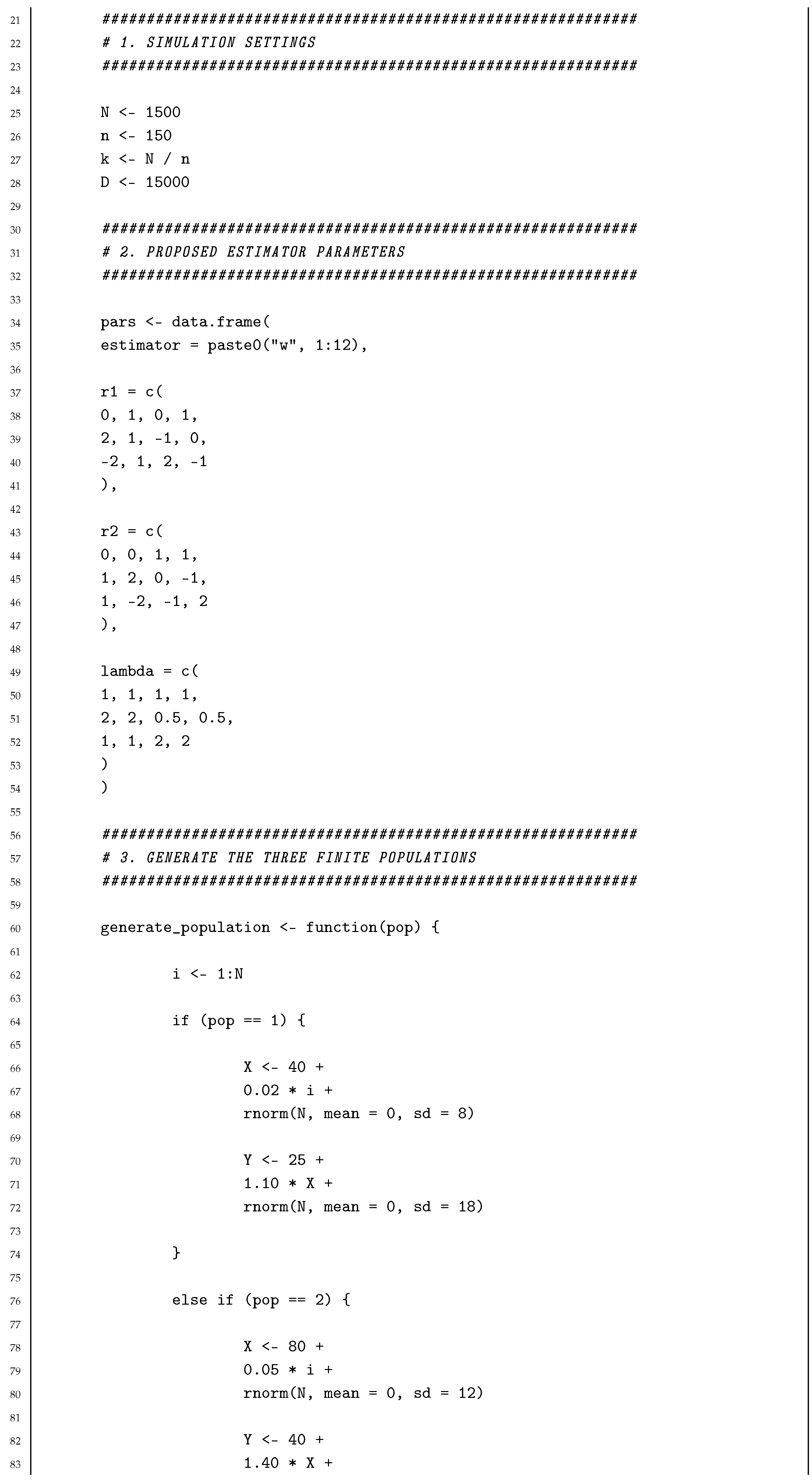
Three finite populations are generated to evaluate the performance of the proposed estimator relative to the existing estimators in terms of mean squared error. Each population contains ordered units, with the units indexed by
For each population, the auxiliary variable is generated by combining a linear trend with a normally distributed random error. The study variable is then generated as a linear function of with an additional normally distributed error term. All random error terms are assumed to be mutually independent.
7.2.1. Population 1: Weak Trend and Moderate Association
The auxiliary variable is generated as
where
The corresponding study variable is generated as
where
Population-l represents a population with a weak increasing trend, relatively low variability, and a moderate positive association between the study and auxiliary variables.
7.2.2. Population 2: Moderate Trend and Strong Association
The auxiliary variable is generated as
where
The corresponding study variable is generated as
where
Population-ll represents a population with a moderate increasing trend, moderate variability, and a strong positive association between the study and auxiliary variables.
7.2.3. Population 3: Strong Trend and Very Strong Association
The auxiliary variable is generated as
where
The corresponding study variable is generated as
where
Population-lll represents a population with a strong increasing trend, relatively high variability, and a very strong positive association between the study and auxiliary variables.
The parameter values used to generate the three populations are summarized in Table 3.
Table 3.
Parameter specifications of the generated populations.
The three populations differ in their mean levels, trend strengths, variabilities, and degrees of association between Y and X. These differences provide suitable conditions for evaluating the performance of the proposed estimator under different ordered population structures.
7.3. Simulation Scope and Limitation
The simulation study primarily considers positive associations between the study variable Y and the auxiliary variable X. Specifically, the three simulated populations represent moderate, strong, and very strong positive associations, respectively. Although Population 1 has a weak increasing trend, it still represents a positive association between X and Y and should not be interpreted as a zero or negative correlation setting. The present simulation design does not explicitly investigate zero or negative correlations, nor does it systematically consider nonlinear or highly periodic X–Y relationships. Therefore, the reported simulation results should be interpreted within the range of dependence structures considered here. An extended simulation study covering weak, zero, and negative correlations, together with nonlinear and highly periodic population structures, would provide a useful direction for future research.
7.4. Simulation Algorithm
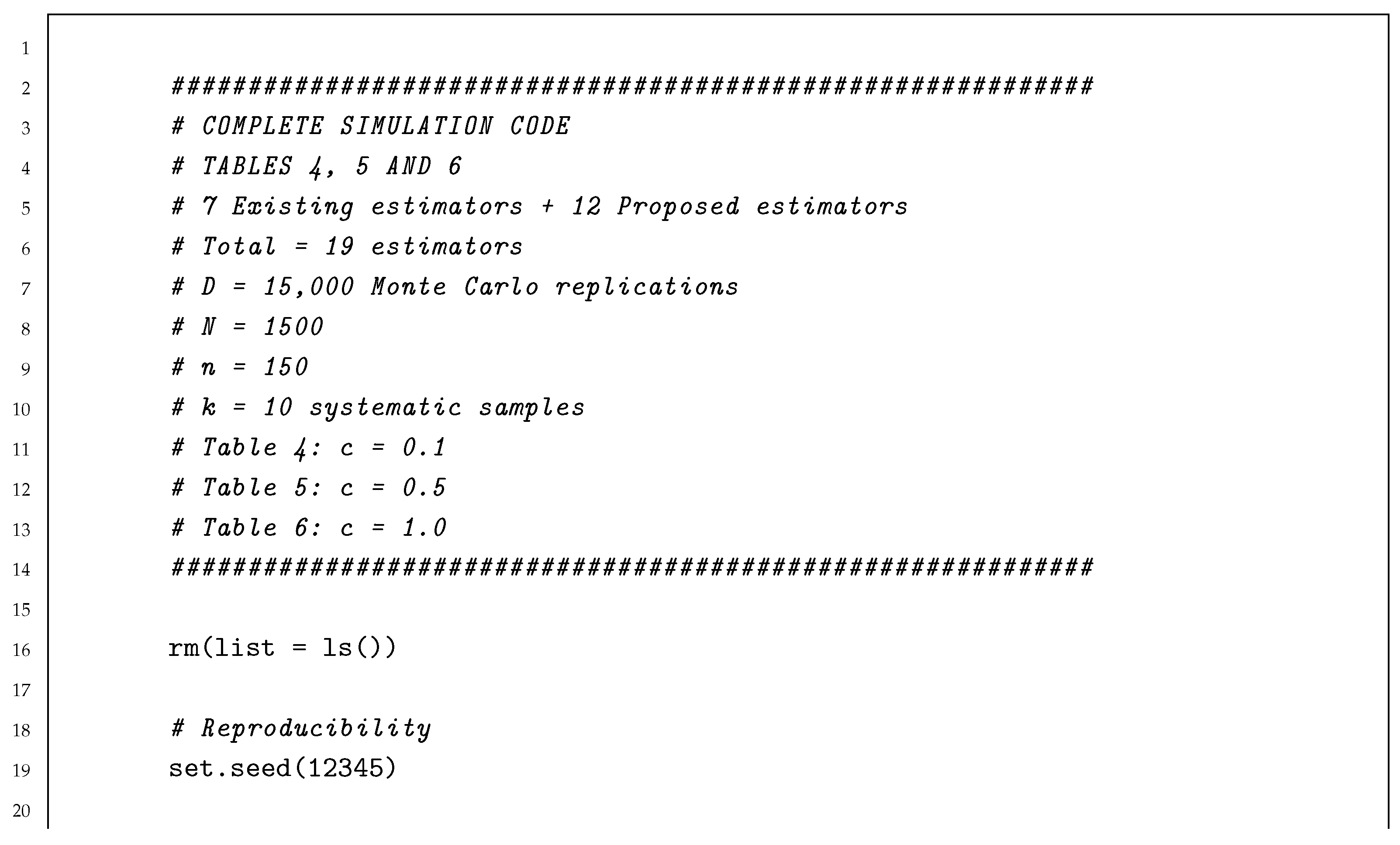
A fixed random seed of 12,345 is used at the beginning of the Monte Carlo simulation to ensure that the simulation results are reproducible. The simulation procedure is carried out according to the following steps.
- Generate a finite population according to one of the population models described above, with population size .
- Set the sample size to and calculate the systematic sampling interval as
- For the generated finite population, consider all possible systematic starting pointsFor each starting point d, the corresponding systematic sample isThus, each generated finite population produces exactly distinct systematic samples.
- For each of the 10 systematic samples, calculate the proposed estimators and all competing estimators.
- For each estimator, calculate the estimation error by comparing its estimate with the corresponding true finite-population mean.
- Repeat Steps 1–5 for 15,000 independently generated finite populations. Thus, the simulation consists of 15,000 independently generated finite populations, with 10 systematic samples evaluated for each population.
- Calculate the empirical mean squared error (MSE) of each estimator by averaging the squared estimation errors over all 15,000 generated populations and all 10 systematic starting points. Thus, the empirical MSE is calculated aswhere denotes the estimate obtained from starting point d in the mth generated population, and is the corresponding true finite-population mean.
7.5. Performance Measures
The percent relative efficiency (PRE) is used to assess the relative performance of each estimator and is calculated based on the ratio of the MSE of the benchmark estimator to the MSE of the estimator under consideration:
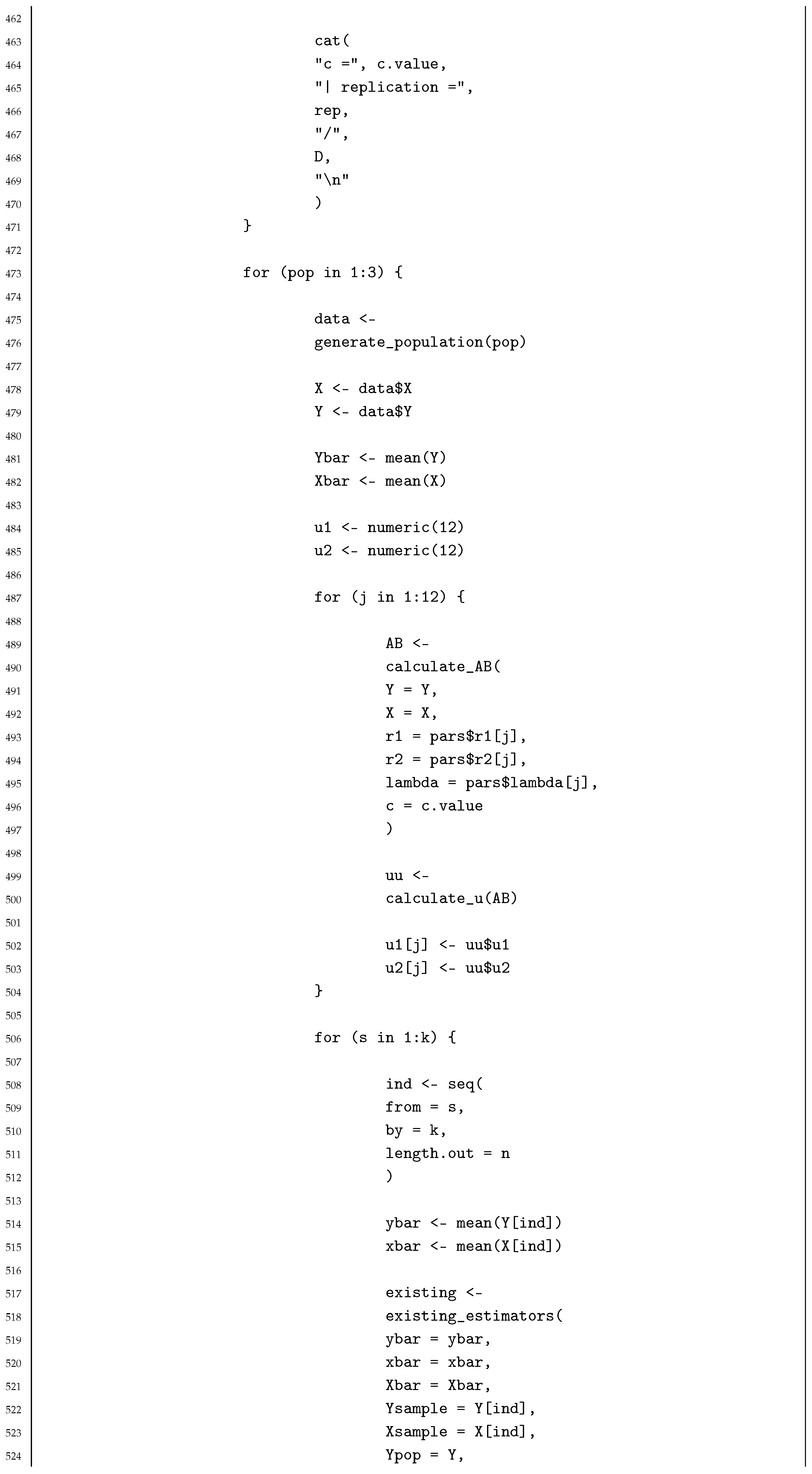
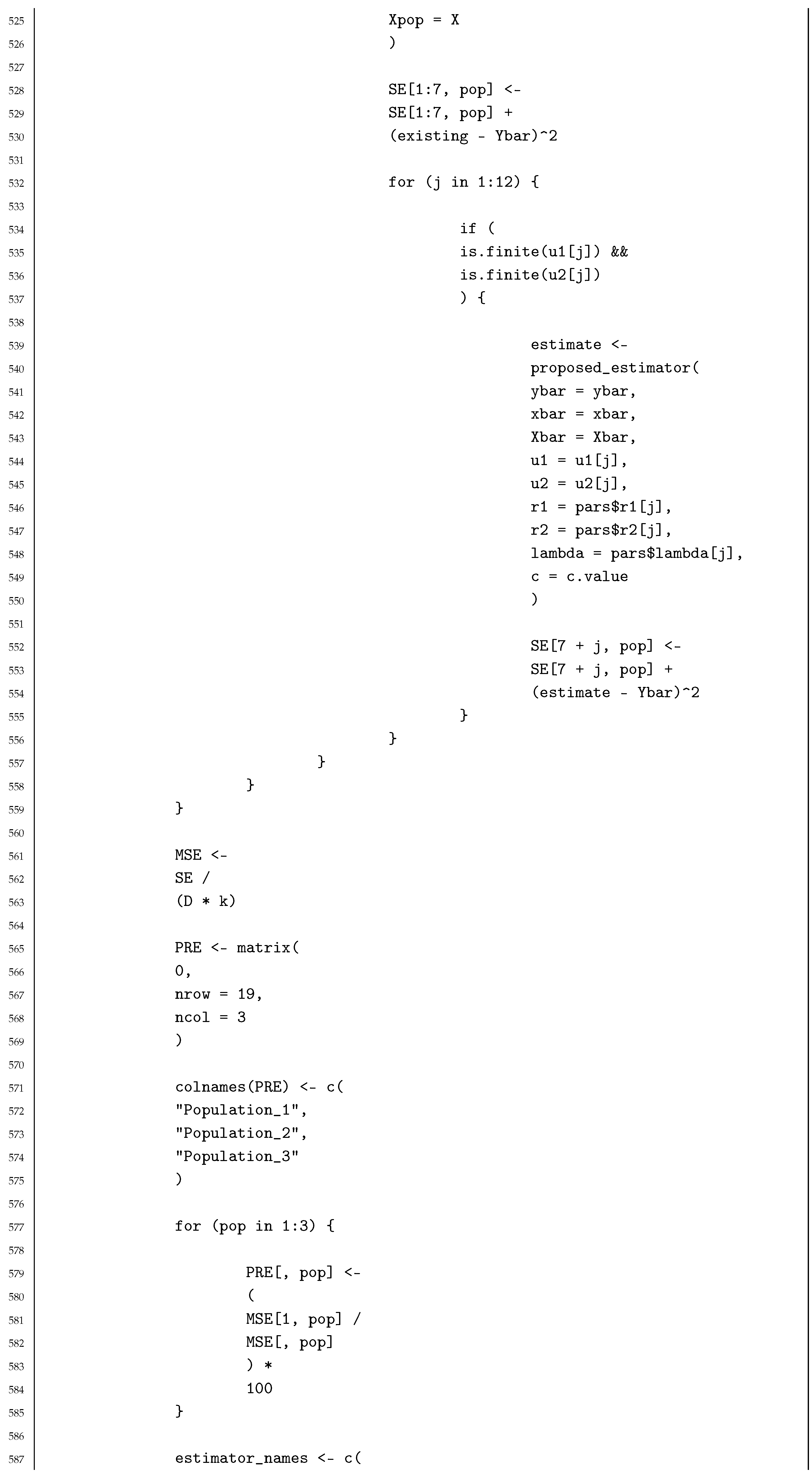
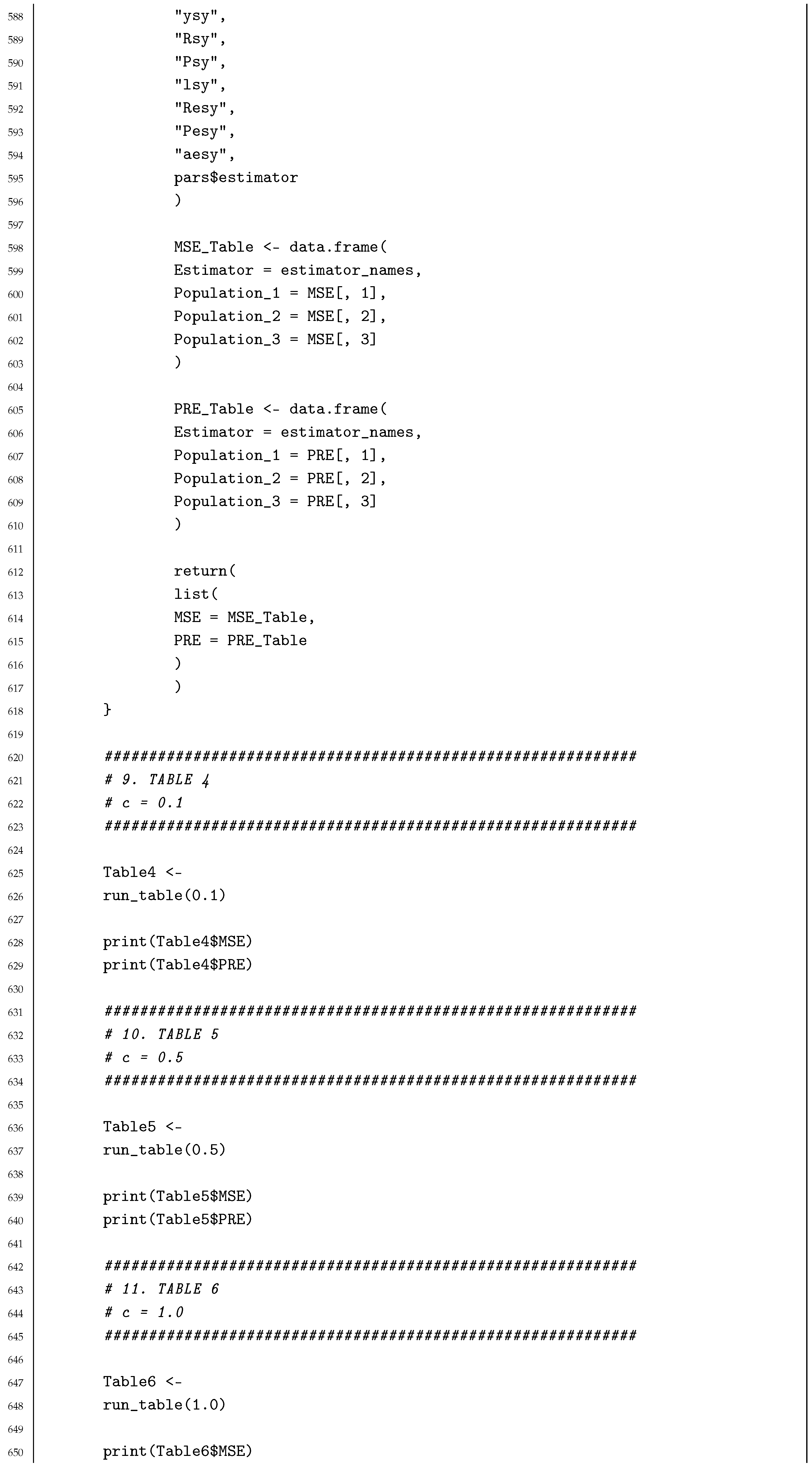
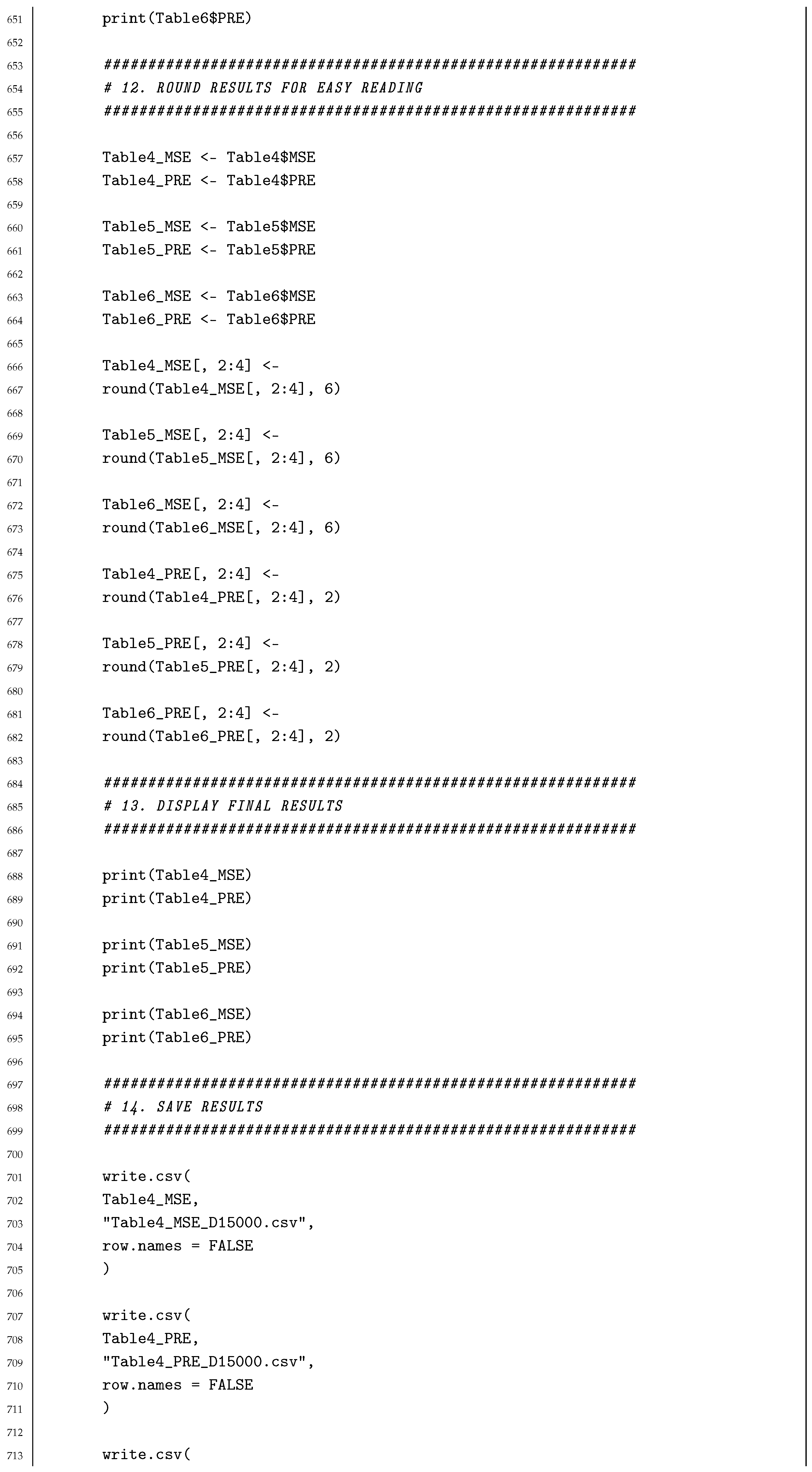
where For reproducibility, the simulation codes are provided in Appendix A.
7.6. Empirical Study
For the empirical investigation, three independent benchmark populations are employed to assess and compare the performance of the proposed estimators. These populations represent different data characteristics and levels of variability, allowing the proposed methodology to be examined under a range of practical settings. Using multiple benchmark populations provides a more comprehensive evaluation and demonstrates that the performance of the proposed estimators is not limited to a single population structure. All empirical results presented in this study are based on analyses carried out using these three populations.
Population 1.
The first population used for the empirical evaluation is obtained from Punjab Development Statistics 2014 (pp. 135–136, Tables 89–90) [31], which reports government school statistics for the academic year 2012–2013. In this population, the study variable (Y) is the total number of registered students at the primary and middle levels, whereas the auxiliary variable (X) is the total number of government schools (primary and middle, combined for both boys and girls). These variables are used to evaluate the performance of the proposed estimators under the systematic sampling framework. The corresponding summary statistics are presented below.
Population 2.
The second population used for the empirical evaluation is obtained from the Punjab Development Statistics 2013 (p. 226, Table 158) [32], which provides district-level information on employment and industrial activity for the years 2010 and 2012. In this population, the study variable (Y) is the district-level employment, while the auxiliary variable (X) is the number of registered factories in each district. These variables are employed to evaluate the performance of the proposed estimators under the systematic sampling framework. The corresponding summary statistics are presented below.
Population 3.
Represents the medical education sector of Punjab, where each unit corresponds to a district or institution-level observation. The study variable Y denotes the number of medical institutions, while the auxiliary variable X represents the number of teaching staff in medical institutes. The auxiliary variable provides information about the human resource capacity of the medical education system and is used to improve the estimation of the study variable. Both variables are obtained from Education-Professional/Medical Institutes (pp. 129–132, Table 86) [31], and are used to improve estimation efficiency under systematic sampling. The summary statistics are defined as follows:
8. Results and Discussion
The proposed family of mean-based estimators underwent evaluation through both simulation and empirical investigations under systematic sampling. The simulation study examined the influence of the transformation parameters together with the exponential adjustment parameter c, whereas the empirical investigation assessed the practical performance of the proposed family using three benchmark populations.
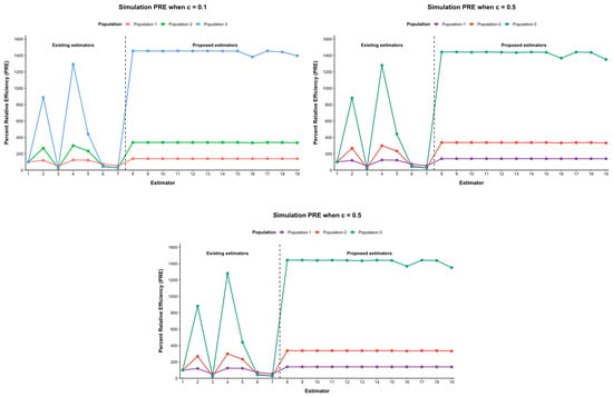
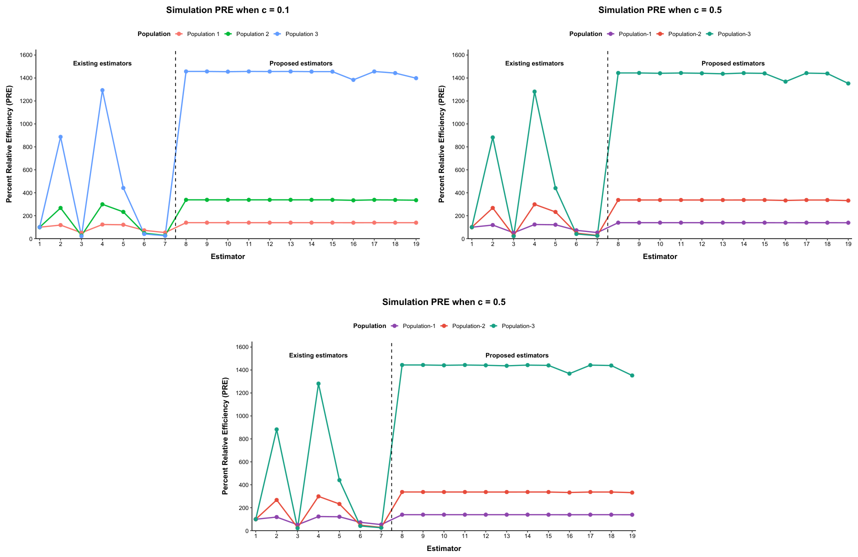
Table 4, Table 5 and Table 6 summarize the simulation results corresponding to , , and . The results indicate that the proposed subclasses generally achieve higher PRE values than the existing estimators across the generated populations. Among the existing estimators, the adjusted exponential estimator generally provides the most favorable PRE performance, whereas the product estimator and the exponential product estimator tend to produce comparatively lower PRE values. The proposed subclasses show substantially higher PRE values for several parameter combinations, demonstrating the potential benefit of combining power transformations with the exponential adjustment. Figure 1 provides a graphical presentation of these findings and distinguishes the proposed estimators from the existing methods. The results also show that the PRE values vary with the value of c, indicating that the exponential adjustment parameter influences the relative efficiency of the proposed estimators within the range considered.
Table 4.
Sensitivity Analysis of PRE under Systematic Sampling.
Table 5.
Sensitivity Analysis of PRE under Systematic Sampling.
Table 6.
Sensitivity Analysis of PRE under Systematic Sampling.
Figure 1.
Graphical representation of the simulation results obtained under different populations. Estimator numbers 1–7 represent the existing estimators, while numbers 8–19 represent the proposed estimators.
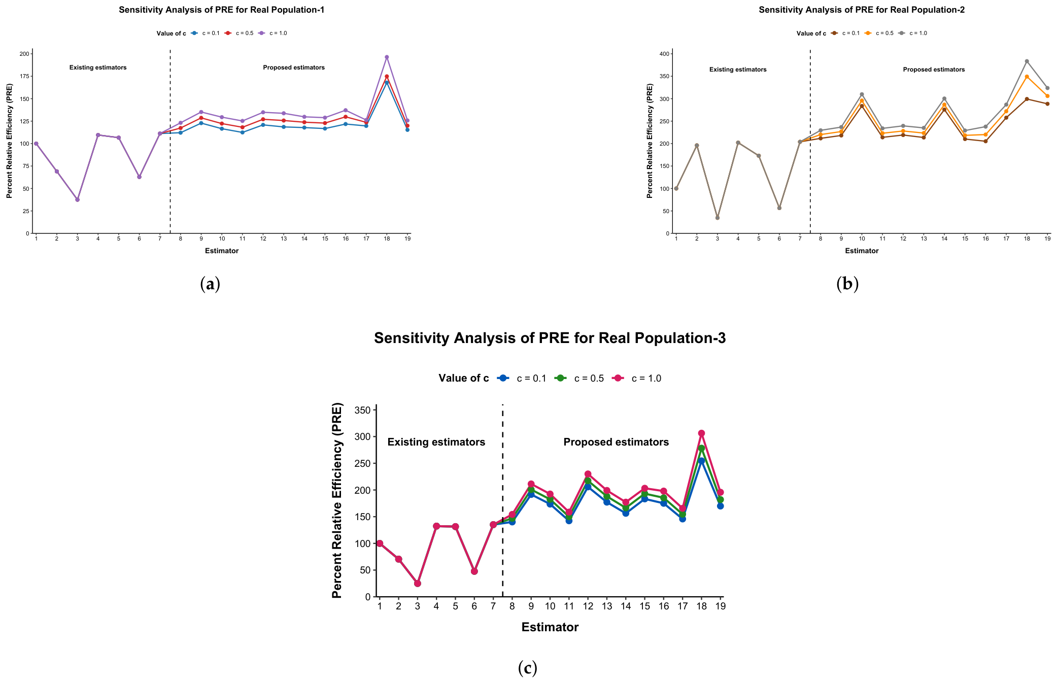
Table 7, Table 8 and Table 9 present the empirical results for the three benchmark populations in terms of PRE. The results demonstrate noticeable differences in relative efficiency across the populations and parameter combinations. For Population 1, the proposed estimators generally provide higher PRE values than most existing estimators, with providing the highest PRE among the proposed subclasses across the considered values of c. Similarly, for Population 2, provides the highest PRE among the proposed estimators, followed by for the considered settings. For Population 3, the proposed subclasses also attain high PRE values for several parameter combinations, although their relative performance varies more noticeably across the different values of c. Overall, the empirical results indicate that provides particularly strong relative efficiency across the three benchmark populations, while the remaining proposed subclasses show varying degrees of improvement depending on the population characteristics and parameter settings.
Table 7.
Sensitivity Analysis of PRE under Systematic Sampling for Real Populations.
Table 8.
Sensitivity Analysis of PRE under Systematic Sampling for Real Populations.
Table 9.
Sensitivity Analysis of PRE under Systematic Sampling for Real Populations.
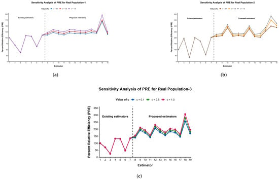
Figure 2 illustrates the empirical PRE results for Populations 1, 2, and 3, respectively. The figures show the variation in relative efficiency among the existing and proposed estimators and demonstrate that several proposed subclasses achieve substantially higher PRE values than the existing methods. Although the magnitude of PRE differs across the three benchmark populations, the proposed family generally provides favorable relative efficiency, with emerging as one of the strongest proposed subclasses. These empirical findings support the effectiveness of the proposed family while also indicating that the relative performance of individual subclasses depends on the population characteristics and the selected transformation parameters.
Figure 2.
Real population results across different estimators, where estimators 1–7 represent existing methods and estimators 8–19 represent the proposed methods.
9. Conclusions
This study proposed a new family of mean-based estimators for estimating the population mean under systematic sampling by combining power transformations with an exponential adjustment. General expressions for the bias and mean squared error were derived using the first-order approximation, and the optimum values of the unknown constants were obtained by minimizing the mean squared error. The proposed formulation provides a unified framework that accommodates different transformation structures through suitable choices of the parameters and the exponential adjustment parameter c.
Both the oracle-based simulation and empirical efficiency evaluations demonstrated the effectiveness of the proposed family. Across the generated and benchmark populations, the proposed subclasses consistently achieved smaller mean squared errors than the existing estimators considered in this study. The sensitivity analysis indicated that the effect of the exponential adjustment parameter on relative efficiency depends on the estimator and population characteristics within the selected range, while the empirical investigation confirmed that the proposed estimators maintained their superiority under different practical population characteristics. These findings suggest that the proposed family provides a reliable and flexible alternative for population mean estimation when auxiliary information is available under systematic sampling.
Although the proposed family performed well under the scenarios considered in this study, further investigation remains worthwhile. Future research may extend the proposed methodology to other sampling designs, including stratified systematic sampling, two-phase sampling, and adaptive sampling. Additional studies may also examine its performance in the presence of non-response, measurement errors, missing observations, or influential observations. Another promising direction involves developing data-driven procedures for selecting the transformation parameters, which may further improve the practical applicability of the proposed family in complex survey sampling problems.
Author Contributions
Conceptualization, H.A. and F.A.A.; Methodology, H.A. and F.A.A.; Software, H.A. and F.A.A.; Validation, H.A. and F.A.A.; Formal analysis, H.A. and F.A.A.; Investigation, H.A. and F.A.A.; Resources, H.A.; Data curation, H.A. and F.A.A.; Writing—original draft, H.A.; Writing—review and editing, H.A. and F.A.A.; Visualization, H.A. and F.A.A.; Supervision, F.A.A.; Project administration, H.A. and F.A.A.; Funding acquisition, F.A.A. All authors have read and agreed to the published version of the manuscript.
Funding
The authors extend their appreciation to the Deanship of Scientific Research and Libraries in Princess Nourah bint Abdulrahman University for funding this research work through the Suporting Publication in Top-impact journals Initiative (SPTIF-2026).
Data Availability Statement
The original contributions presented in this study are included in the article. Further inquiries can be directed to the corresponding author.
Conflicts of Interest
The authors declare no conflicts of interest.
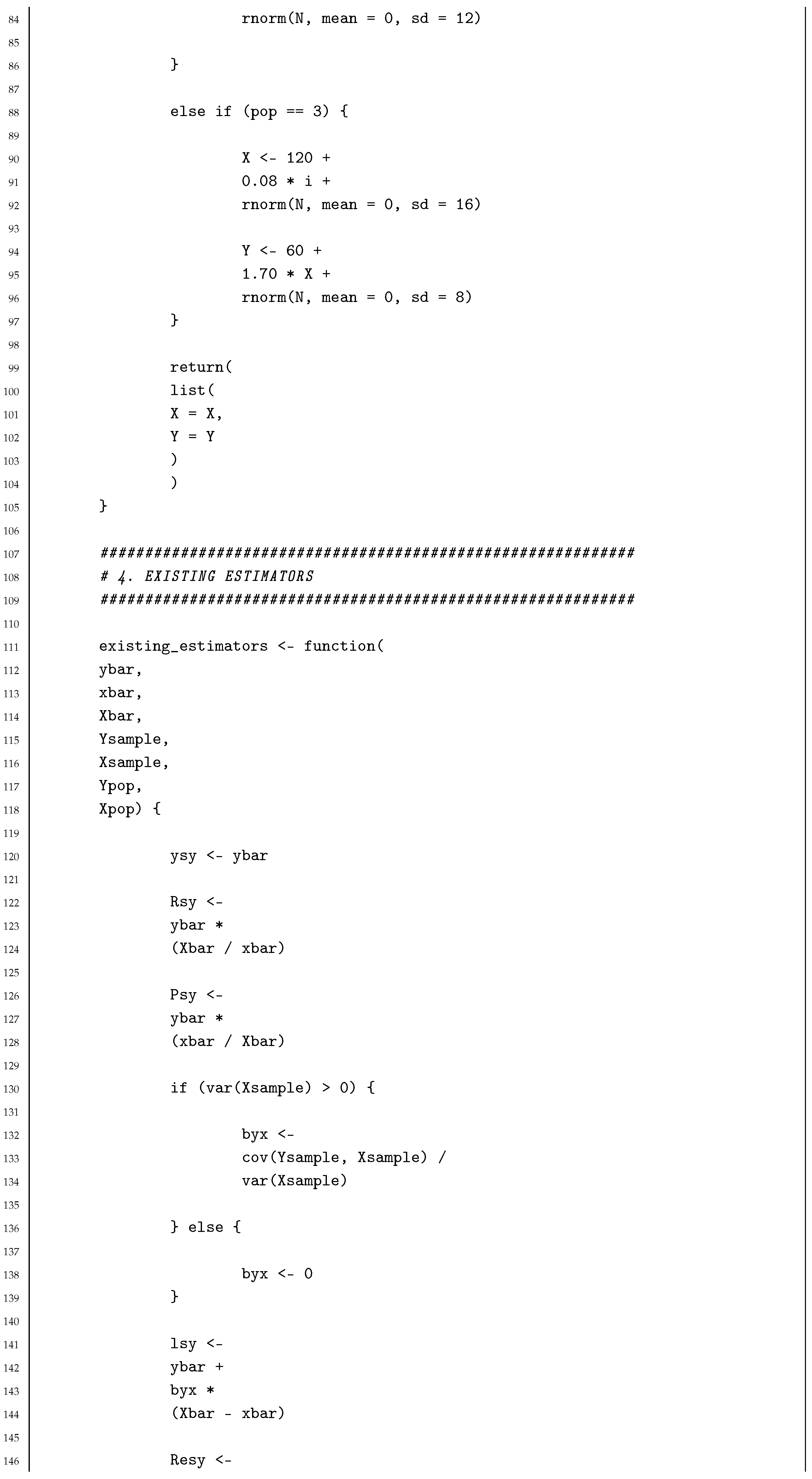
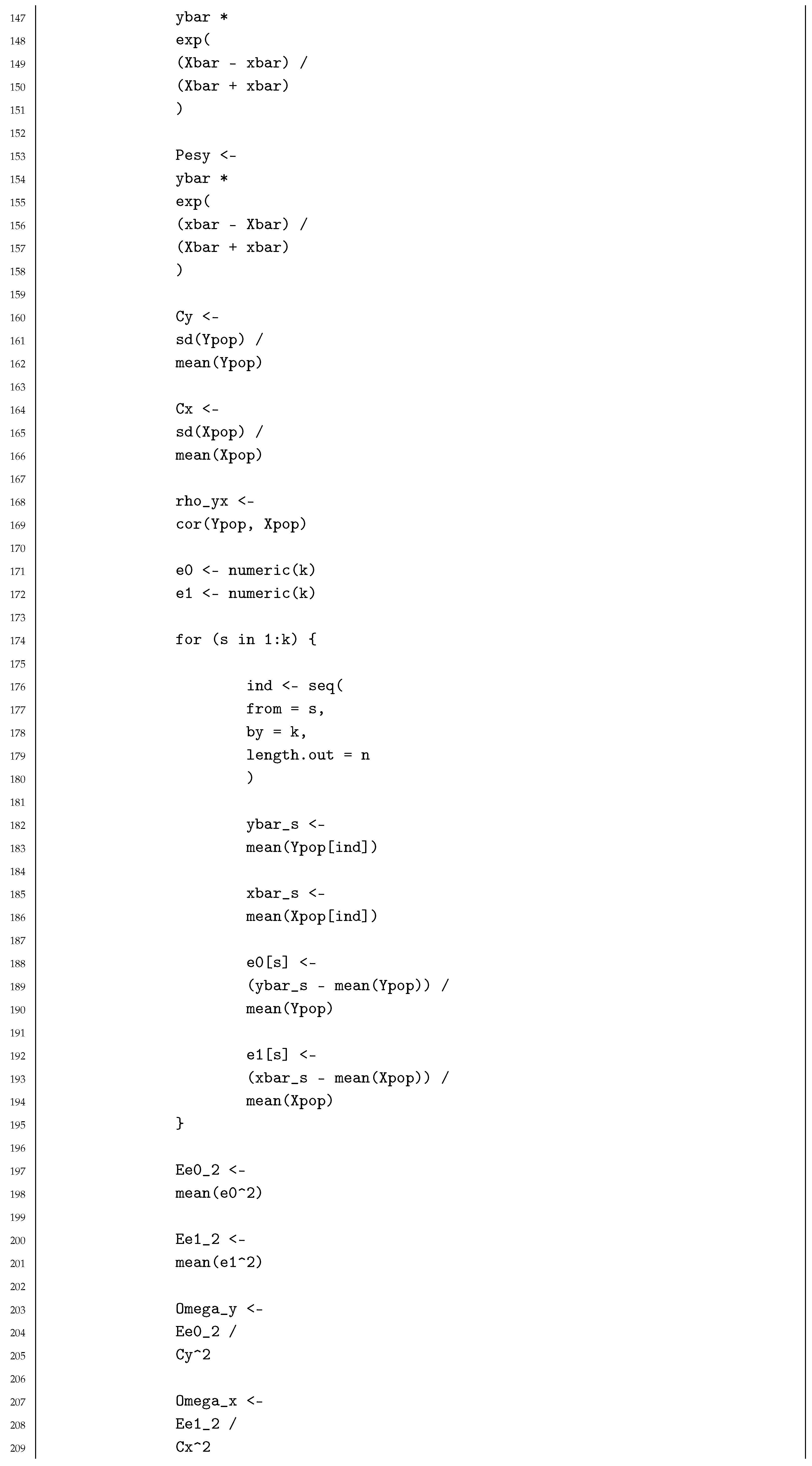
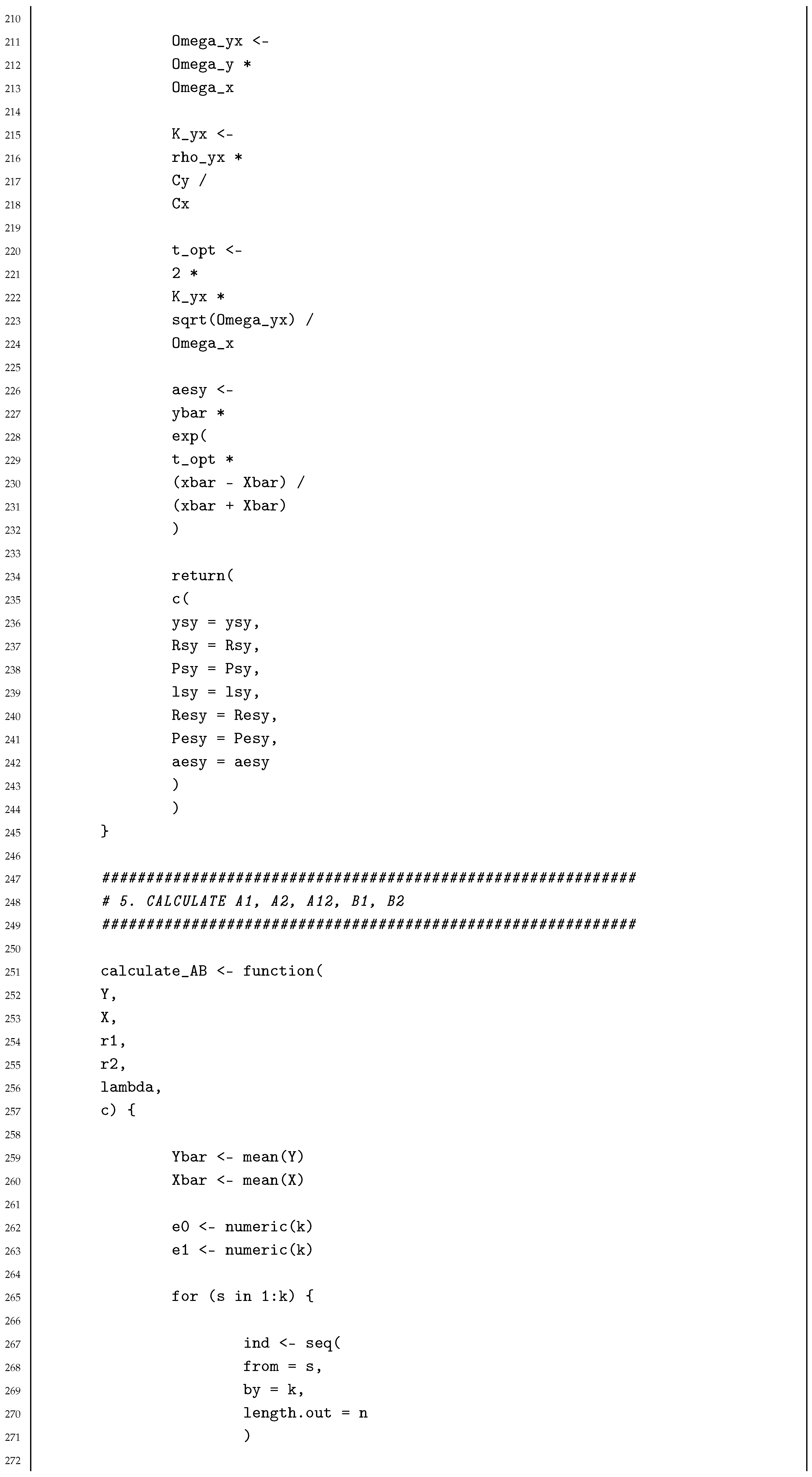
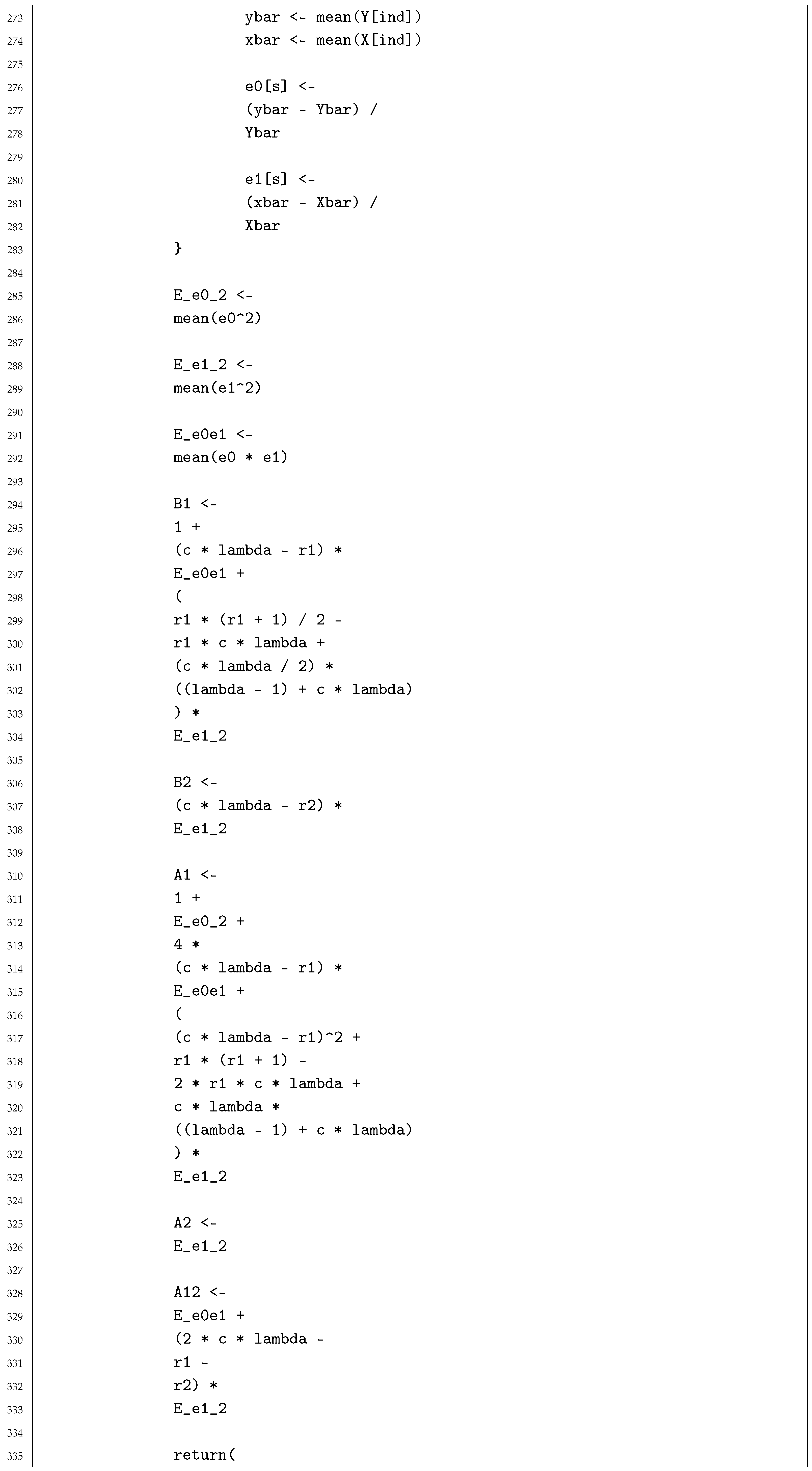
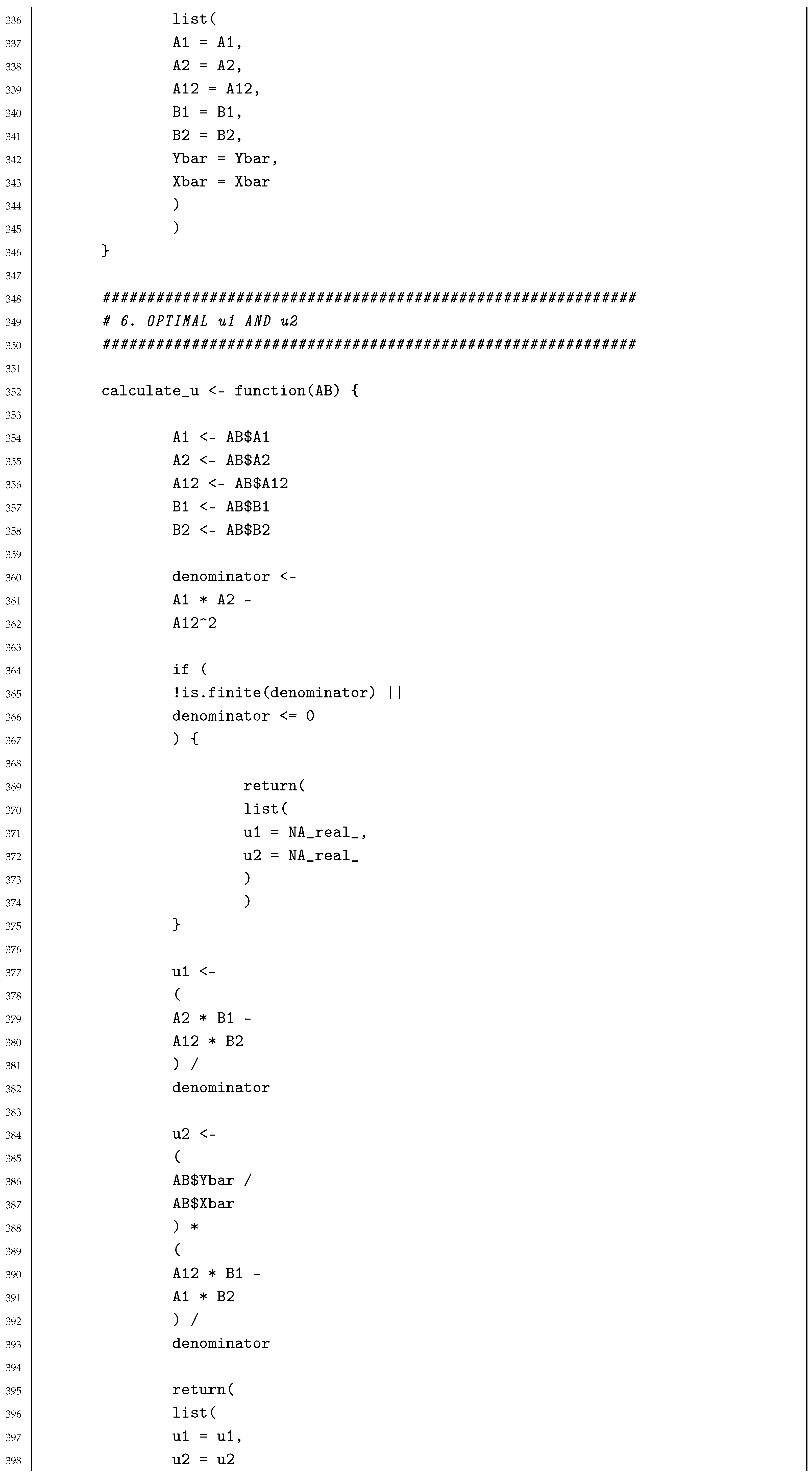
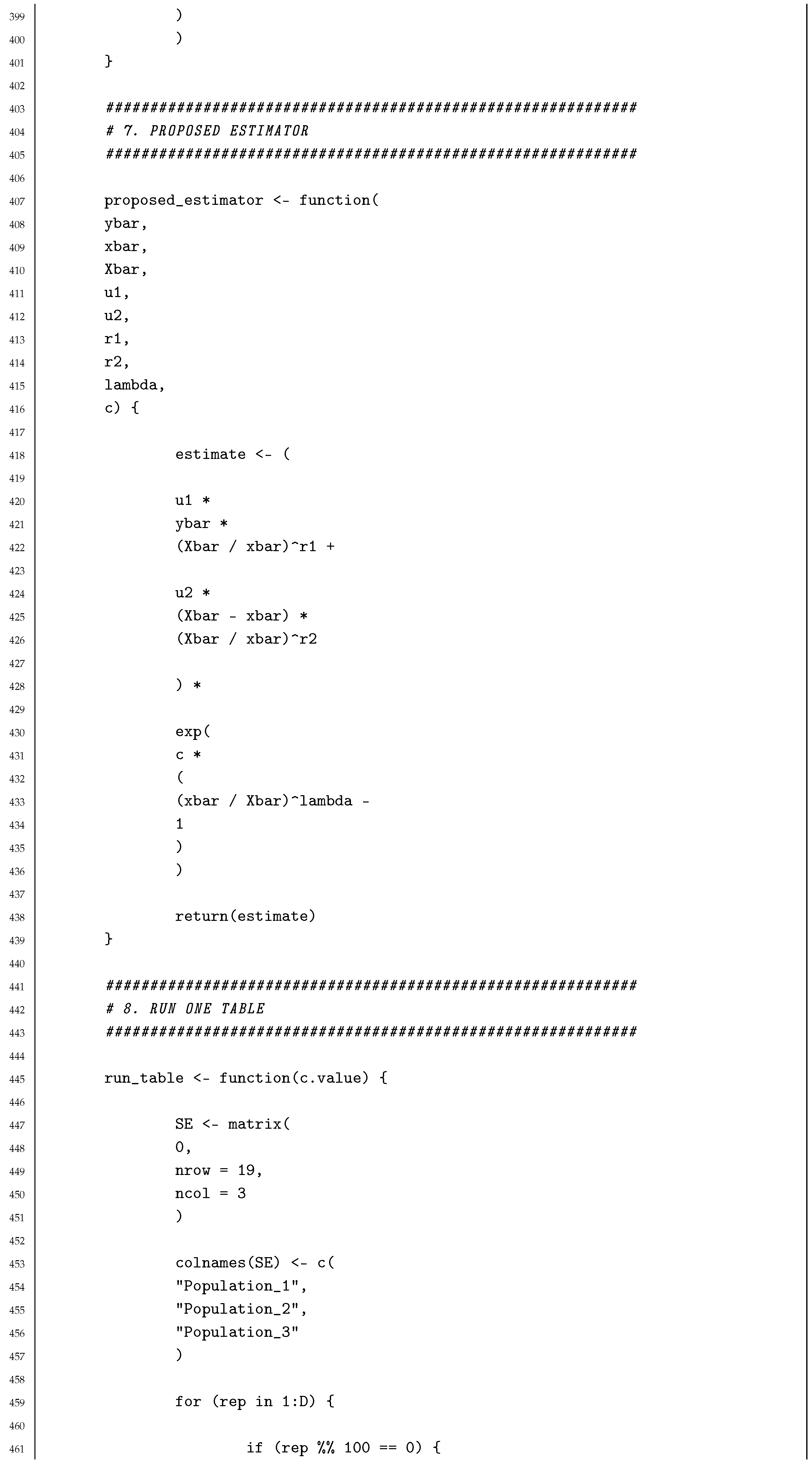
Appendix A. R Code for the Monte Carlo Simulation
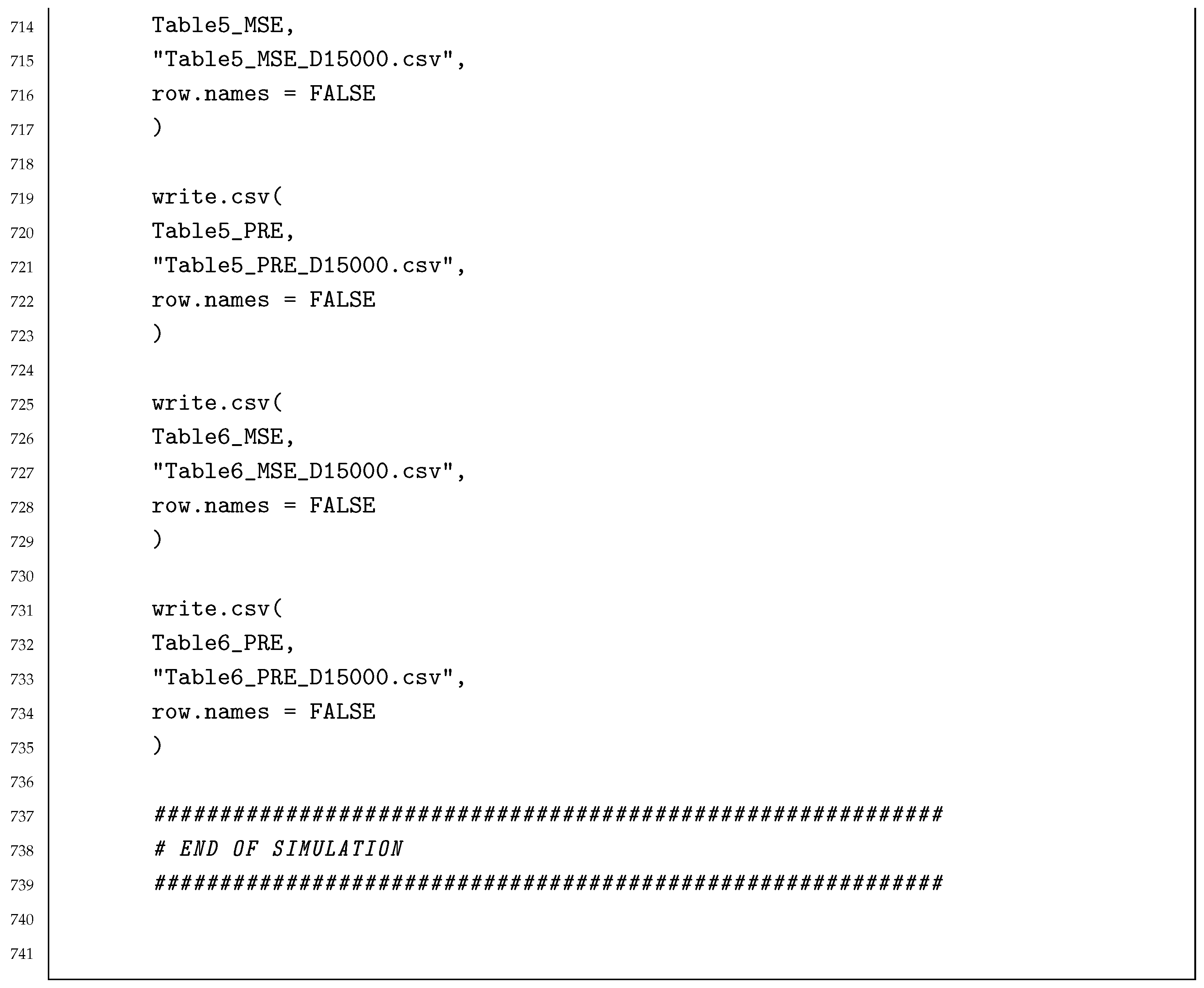
The following R code was used to perform the Monte Carlo simulation reported in Table 5 and Table 6. The simulation uses Monte Carlo replications, a finite population size , sample size , and possible systematic samples. The random seed is set to 12,345 to ensure reproducibility.
References
- Cochran, W.G. Relative efficiency of systematic and stratified random samples for a certain class of population. Ann. Math. Stat. 1946, 17, 164–177. [Google Scholar] [CrossRef] [Scilit]
- Yates, F. Systematic sampling. Philos. Trans. R. Soc. Lond. Ser. A 1948, 241, 345–377. [Google Scholar] [CrossRef] [Scilit]
- Madow, W.G. On the theory of systematic sampling. Ann. Math. Stat. 1948, 19, 333–354. [Google Scholar] [CrossRef] [Scilit]
- Gautschi, W. Some remarks on systematic sampling. Ann. Math. Stat. 1957, 28, 385–394. [Google Scholar] [CrossRef] [Scilit]
- Hajeck, J. Optimum strategy and other problems in probability sampling. Čas. Pěst. Mat. 1959, 84, 387–423. [Google Scholar] [CrossRef] [Scilit]
- Kish, L. Survey Sampling; John Wiley & Sons: New York, NY, USA, 1965. [Google Scholar]
- Murthy, M.N. Sampling Theory and Methods, 2nd ed.; Statistical Publishing Society: Calcutta, India, 1967. [Google Scholar]
- Cochran, W.G. Sampling Techniques, 3rd ed.; John Wiley and Sons: Hoboken, NJ, USA, 1977. [Google Scholar]
- Hansen, M.H.; Hurwitz, W.N. On the theory of sampling from finite populations. Ann. Math. Stat. 1943, 14, 333–362. [Google Scholar] [CrossRef] [Scilit]
- Lahiri, D.B. On the question of bias of systematic sampling. Proc. World Pet. Congr. 1954, 6, 349–362. [Google Scholar]
- Swain, A.K.P.C. The use of systematic sampling in ratio estimate. J. Ind. Stat. Assoc. 1964, 2, 160–164. [Google Scholar]
- Shukla, N.D. Systematic sampling and product method of estimation. In Proceedings of the All-India Seminar on Demography and Statistics; BHU: Varanasi, India, 1971. [Google Scholar]
- Kushwaha, K.S.; Singh, H.P. Class of almost unbiased ratio and product estimators in systematic sampling. J. Indian Soc. Agric. Stat. 1989, 41, 193–205. [Google Scholar]
- Kushwaha, S.N.S.; Kushwaha, K.S. A class of ratio, product and difference (RPD) estimators in systematic sampling. Microelectron. Reliab. 1993, 33, 455–457. [Google Scholar] [CrossRef] [Scilit]
- Singh, R.; Singh, H.P. Almost unbiased ratio and product-type estimators in systematic sampling. Qüestiió 1998, 22, 403–416. [Google Scholar]
- Singh, H.P.; Tailor, R.; Jatwa, N.K. Modified ratio and product estimators for population mean in systematic sampling. Mod. Appl. Stat. Methods 2011, 10, 424–435. [Google Scholar] [CrossRef] [Scilit]
- Singh, H.P.; Solanki, R.S. An efficient class of estimators for the population mean using auxiliary information in systematic sampling. J. Stat. Theory Pract. 2012, 6, 274–285. [Google Scholar] [CrossRef] [Scilit]
- Tailor, T.; Jatwa, N.K.; Singh, H.P. A ratio-cum-product estimator of finite population mean in systematic sampling. Stat. Transit. 2013, 14, 391–398. [Google Scholar] [CrossRef] [Scilit]
- Singh, H.P.; Jatwa, N.K. A class of exponential type estimators in systematic sampling. Econ. Qual. Control 2013, 27, 195–208. [Google Scholar] [CrossRef] [Scilit]
- Khan, M.; Singh, R. Estimation of population mean in chain ratio-type estimator under systematic sampling. J. Probab. Stat. 2015, 2015, 248374. [Google Scholar] [CrossRef] [Scilit]
- Noor-ul-Amin, M.; Javaid, A.; Hanif, M. Estimation of population mean in systematic random sampling using auxiliary information. J. Stat. Manag. Syst. 2017, 20, 1095–1106. [Google Scholar] [CrossRef] [Scilit]
- Javaid, A.; Noor-ul-Amin, M.; Hanif, M. Modified ratio estimator in systematic random sampling under non-response. Proc. Natl. Acad. Sci. India Sect. A Phys. Sci. 2019, 89, 817–825. [Google Scholar] [CrossRef] [Scilit]
- Qureshi, M.N.; Khalil, S.; Hanif, M. Generalized semi exponential type estimator under systematic sampling. J. Stat. Theory Appl. 2018, 17, 283–290. [Google Scholar] [CrossRef] [Scilit]
- Khan, M.; Shabbir, J. Some improved ratio, product, and regression estimators of finite population mean using minimum and maximum values. Sci. World J. 2013, 2013, 431868. [Google Scholar] [CrossRef] [Scilit] [PubMed]
- Iftikhar, A.; Shi, H.; Hussain, S.; Qayyum, A.; El-Morshedy, M.; Al-Marzouki, S. Estimation of finite population mean in presence of maximum and minimum values under systematic sampling scheme. AIMS Math. 2022, 7, 9825–9834. [Google Scholar] [CrossRef] [Scilit]
- El-Morshedy, M.; Hussain, S.; Ullah, K.; Khalil, A.; Shabbir, J.; Mansoor, W. Finite population mean estimation under systematic sampling scheme in presence of maximum and minimum values using two auxiliary variables. Math. Probl. Eng. 2022, 2022, 2703178. [Google Scholar] [CrossRef] [Scilit]
- Koçyiğit, E.G. New memory-type estimators for systematic sampling. J. Adv. Res. Nat. Appl. Sci. 2025, 11, 224–236. [Google Scholar] [CrossRef] [Scilit]
- Karim, A.; Khan, H.; Mahmood, Y.; Riaz, M.; Ahmad, S. On estimation and monitoring of population mean using systematic sampling under an exponentially weighted moving average scheme. Pak. J. Stat. Oper. Res. 2024, 20, 517–531. [Google Scholar] [CrossRef] [Scilit]
- Pal, S.K.; Mahmud, S.A.; Singh, H.P. An efficient estimation of finite population mean through difference estimator in systematic sampling. Afr. Mat. 2025, 36, 14. [Google Scholar] [CrossRef] [Scilit]
- Nagy, M.; Qureshi, M.N.; Shaheen, N.; Hanif, M. Mean estimation using memory-type estimators in systematic sampling for time-scaled surveys. Math 2026, 14, 1180. [Google Scholar] [CrossRef] [Scilit]
- Bureau of Statistics. Punjab Development Statistics Government of the Punjab, Lahore, Pakistan; Bureau of Statistics: Islamabad, Pakistan, 2014.
- Bureau of Statistics. Punjab Development Statistics Government of the Punjab, Lahore, Pakistan; Bureau of Statistics: Islamabad, Pakistan, 2013.

Disclaimer/Publisher’s Note: The statements, opinions and data contained in all publications are solely those of the individual author(s) and contributor(s) and not of MDPI and/or the editor(s). MDPI and/or the editor(s) disclaim responsibility for any injury to people or property resulting from any ideas, methods, instructions or products referred to in the content. |
© 2026 by the authors. Licensee MDPI, Basel, Switzerland. This article is an open access article distributed under the terms and conditions of the Creative Commons Attribution (CC BY) license.