Fuzzy Aura Topological Spaces: Čech Closure Operators, Generalized Open Sets, and Rough Approximation

Abstract

We introduce a fuzzy aura topological space$(X,\tilde{\tau },\tilde{a})$: a Chang-type fuzzy topological space carrying a fuzzy scope function $\tilde{a}:X\to \tilde{\tau }$ with $\tilde{a}\left(x\right)\left(x\right)=1$, generalizing the crisp aura spaces. The scope function is a graded, per-point observation window; narrowing it turns the induced rough approximation into a variable-resolution model whose boundary shrinks as the window sharpens (refinement monotonicity), illustrated by closed-form multi-resolution segmentation examples on the line and in the plane. The fuzzy aura-closure ${\mathrm{cl}}_{\tilde{a}}$ is a fuzzy additive Čech closure operator; it need not be idempotent, but its countable iteration is a fuzzy Kuratowski closure with the same fixed points, so both operators induce one fuzzy aura topology ${\tilde{\tau }}_{\tilde{a}}$, which, unlike in the crisp theory, need not be contained in $\tilde{\tau }$. We introduce five classes of generalized fuzzy open sets forming a strict hierarchy, study fuzzy $\tilde{a}$-continuity and its decompositions, and define separation axioms fuzzy $\tilde{a}$-$T_i$ ($i=0,1,2$) and fuzzy $\tilde{a}$-regularity that depend on the scope function rather than the topology, together with a graded level variant of $T_1$ suited to continuous scope functions. The approximation operators coincide with the Dubois–Prade pair of the associated reflexive fuzzy relation and recover the Pawlak and crisp aura models as special cases.

1. Introduction

Topological spaces are often equipped with an auxiliary set-theoretic structure. Ideal topological spaces $(X,\tau ,\mathcal{I})$, rooted in the work of Kuratowski [1] and Vaidyanathaswamy [2], were systematically developed by Janković and Hamlett [3]. Dual and related structures, namely filters (Cartan [4]), grills (Choquet [5], Roy and Mukherjee [6], Al-Omari and Noiri [7]), and the recent primals (Acharjee, Özkoç, and Issaka [8]), have each led to their own closure operators and derived topologies; Al-Omari and Alqahtani [9] developed the closure-operator side of primal structures in detail, and Alghamdi [10] carried compactness into the primal setting.

Alongside these crisp developments, topology has been combined with fuzzy sets (Zadeh [11], Chang [12], Lowen [13]), soft sets (Molodtsov [14], Shabir and Naz [15]), and rough sets (Pawlak [16]). Each carries its own topology, and the combinations have been worked out from many angles; El-Bably, Fleifel, and Embaby [17] approached rough approximations through closure operators, Lin [18] recast rough interior and closure operators in categorical terms, and Zhan and Alcantud [19] put soft rough coverings to work on group decision problems. Per-point neighborhood systems remain an active route to rough approximation, as in the cardinality rough neighborhoods of Al-shami et al. [20], while Mareay, Abu-Gdairi, and Badr [21] hybridize the fuzzy and rough sides directly through covering-based soft rough fuzzy sets, and Wang, Xie, and Zhi [22] extend S-approximation spaces to a pair of fuzzy universes. Within fuzzy topology itself, generalized open sets and ideal-based structures continue to be developed, as in the fuzzy maximal $\mu$-open sets of Swaminathan and Sheela [23], the fuzzy ideal supra structures of Abbas [24], and the fuzzy $hI$-open sets that a fuzzy ideal induces [25].

Fuzzy topology and rough sets have a long shared history. Dubois and Prade [26] built fuzzy rough sets from fuzzy relations, Radzikowska and Kerre [27] compared the models that followed, Yao [28] developed the constructive and algebraic sides of the theory, and Chacón-Gómez, Cornejo, and Medina [29] examined how decision rules operate inside fuzzy rough set theory.

Açıkgöz recently introduced the concept of an aura topological space $(X,\tau ,a)$ [30], where a scope function $a:X\to \tau$ with $x\in a\left(x\right)$ assigns to each point a fixed open neighborhood. This simple axiom yields an additive Čech closure operator, five generalized open-set classes, separation axioms depending on the scope function, and a rough set model that requires no equivalence relation.

The present paper generalizes aura topological spaces to the fuzzy setting. Working with Chang-type fuzzy topological spaces [12], we define a fuzzy scope function $\tilde{a}:X\to \tilde{\tau }$ satisfying $\tilde{a}\left(x\right)\left(x\right)=1$ and call the resulting triple $(X,\tilde{\tau },\tilde{a})$ a fuzzy aura topological space. Moving from characteristic functions to membership grades is not just a change of notation. The closure and interior operators behave less rigidly, their link to the ambient topological closure is harder to pin down, and the rough set model must now handle graded uncertainty. Three differences from the crisp theory deserve emphasis at the outset. First, in the crisp case every a-open set is open in the ambient topology, whereas the fuzzy aura topology ${\tilde{\tau }}_{\tilde{a}}$ can escape $\tilde{\tau }$ entirely (Example 6). Second, membership now spreads by degrees: a point can acquire partial closure membership through a cross-aura value even though no crisp intersection forms (Example 5). Third, the scope width becomes a continuously tunable resolution parameter whose effect on the rough boundary is monotone (Theorem 20), something the crisp model can imitate only by discrete refinement.

Why should this matter to a reader outside topology? For work on image or signal segmentation the payoff is concrete: the lower approximation of a foreground is its certain core, the upper approximation is its possible region, and the gap between them is the uncertain edge band, so Theorem 20 says that sharpening the observation window can only shrink that band, never widen it. For granular computing the same statement reads differently: the granulation carried by $\tilde{a}$ can be refined along a continuum, with approximation quality improving monotonically all the way, instead of being switched between finitely many prescribed granulations. Section 7 works this out in closed form, for a one-dimensional signal and for a two-dimensional foreground.

A scope function is best read as a graded observation window: $\tilde{a}\left(x\right)\left(y\right)$ is the degree to which y is visible from x, and $\tilde{a}\left(x\right)\left(x\right)=1$ says each point sees itself sharply. The window is local and it is adjustable, and both properties matter for everything that follows. Narrowing it, for instance by shrinking the width $\sigma$ of a Gaussian aura ${\tilde{a}}_{\sigma }\left(x\right)\left(y\right)=e^{-{(x-y)}^2/{\sigma }^2}$, sharpens the resolution at which a point sees its surroundings, and the induced rough approximation responds monotonically: the boundary region shrinks as the window narrows (Theorem 20). A single model therefore carries a resolution that can be tuned continuously, with the Pawlak, Dubois–Prade, and crisp aura models recovered at particular settings. A fixed ideal or grill cannot do this, because it fixes its auxiliary datum globally, once and for all. Section 7 develops this point, and the worked example on $\mathbb{R}$ there makes the resolution parameter explicit.

We should say plainly where the construction stands relative to fuzzy rough set theory. The two operators studied below are not new ones. Currying a scope function gives a reflexive fuzzy relation $R(x,y)=\tilde{a}\left(x\right)\left(y\right)$, and the fuzzy aura-closure and interior then coincide with the Dubois–Prade upper and lower approximations under R; they do not generalize that pair, and nothing beyond reflexivity enters the identification (Remark 4). The operator theory of such relational approximations is well developed, from the axiomatics of Morsi and Yakout [31] and the constructive theory of Wu, Mi, and Zhang [32] to the correspondence between reflexive transitive fuzzy relations and fuzzy topologies worked out by Qin and Pei [33] and Lai and Zhang [34], and the covering-based fuzzy neighborhood operators of D’eer, Cornelis, and Godo [35]. What the aura structure adds is not the operators but the pairing with an ambient fuzzy topology: the scope values are required to be fuzzy open, and the generalized open sets of Section 4 mix the ambient interior with the aura closure, producing a hierarchy and a failure of the Njåstad $\alpha$-topology property, neither of which has a counterpart on the purely relational side. The separation axioms of Section 6 and the resolution reading of Section 7 are statements about this interplay. Two results below show how much rests on the openness requirement: a fuzzy topological space admits a scope function satisfying the strongest separation axioms precisely when its crisp singletons are fuzzy open (Proposition 8), and on the real line the aura closure acts on triangular and Gaussian profiles by adding widths, so it maps these fuzzy open profiles to fuzzy open profiles (Proposition 6). Concretely, what we claim as new is this: the hierarchy of five mixed classes and the strictness of every inclusion in it (Theorem 9, Example 7); the failure of the Njåstad property, which persists even under transitivity (Remark 12) and blocks the usual topological reading of $\tilde{a}$-$\alpha$-continuity; the scale-additivity law and its consequence that the closure preserves fuzzy openness on the triangular and Gaussian families (Proposition 6); the collapse of the ungraded separation axioms together with the exact criterion for a topology to admit a separating scope function, and the graded level-$\alpha$ axiom that replaces them for continuous auras (Corollary 3, Proposition 8, Definition 18). Each of these statements involves both $\tilde{\tau }$ and $\tilde{a}$, and none of them can be formulated for a bare fuzzy relation.

The paper is organized as follows. Section 2 fixes notation and recalls what we need from fuzzy topology and rough set theory. Section 3 builds the fuzzy aura-closure and interior and the topology they induce, Section 4 the five classes of generalized fuzzy open sets, Section 5 the corresponding continuity notions and their decompositions, and Section 6 the separation axioms, ungraded and graded. Section 7 turns to the rough approximation operators, refinement monotonicity, and the segmentation reading, and Section 8 places the aura beside fuzzy ideals, fuzzy grills, fuzzy closure spaces, fuzzy neighborhood operators, and the Dubois–Prade model. Section 9 closes with the limitations we are aware of and the questions they leave open.

2. Preliminaries

We recall the basic definitions from fuzzy set theory, fuzzy topology, and rough set theory.

2.1. Fuzzy Sets and Fuzzy Topology

Definition 1

([11]). A fuzzy set on a non-empty set X is a function $\mu :X\to [0,1]$. We denote by $I^X$ the collection of all fuzzy sets on X. The fuzzy sets $\overline{0}$ and $\overline{1}$ are defined by $\overline{0}\left(x\right)=0$ and $\overline{1}\left(x\right)=1$ for all $x\in X$.

For fuzzy sets $\mu ,\nu \in I^X$, we write $\mu \le \nu$ if $\mu \left(x\right)\le \nu \left(x\right)$ for all $x\in X$, and define:

$$(\mu \vee \nu )\left(x\right)=max\{\mu \left(x\right),\nu \left(x\right)\},(\mu \wedge \nu )\left(x\right)=min\{\mu \left(x\right),\nu \left(x\right)\},{\mu }^c\left(x\right)=1-\mu \left(x\right).$$

For $\alpha \in [0,1]$, the α-level set of $\mu$ is ${\mu }_{\alpha }=\{x\in X:\mu \left(x\right)\ge \alpha \}$, and the strong α-level set is ${\mu }_{\alpha }^{>}=\{x\in X:\mu \left(x\right)>\alpha \}$.

Definition 2

([12]). A Chang-type fuzzy topology on X is a subcollection $\tilde{\tau }\subseteq I^X$ such that:

(FT1) 

$\overline{0},\overline{1}\in \tilde{\tau }$;

(FT2) 

$\lambda ,\mu \in \tilde{\tau }\Rightarrow \lambda \wedge \mu \in \tilde{\tau }$;

(FT3) 

${\left\{{\lambda }_i\right\}}_{i\in J}\subseteq \tilde{\tau }\Rightarrow {\bigvee }_{i\in J}{\lambda }_i\in \tilde{\tau }$.

Members of $\tilde{\tau }$ are fuzzy open; μ is fuzzy closed if ${\mu }^c\in \tilde{\tau }$.

Definition 3

([12]). Let $(X,\tilde{\tau })$ be a Chang-type fuzzy topological space. The fuzzy closure and fuzzy interior of $\mu \in I^X$ are:

$$\mathrm{cl}\left(\mu \right)=\bigwedge \{\nu \in I^X:\nu \mathit{is}\mathit{fuzzy}\mathit{closed}\mathit{and}\mu \le \nu \},\mathrm{int}\left(\mu \right)=\bigvee \{\lambda \in \tilde{\tau }:\lambda \le \mu \}.$$

Throughout the paper, $\mathrm{cl}$ and $\mathrm{int}$ without a subscript always denote these two ambient operators, computed in $\tilde{\tau }$; the aura operators carry the subscript $\tilde{a}$.

Definition 4.

Let $(X,\tilde{\tau })$ be a fuzzy topological space and $\mu \in I^X$. Then μ is called:

(a) 

fuzzy semi-open [36] if $\mu \le \mathrm{cl}\left(\mathrm{int}\right(\mu \left)\right)$;

(b) 

fuzzy pre-open [37] if $\mu \le \mathrm{int}\left(\mathrm{cl}\right(\mu \left)\right)$;

(c) 

fuzzy $\alpha$-open [37] if $\mu \le \mathrm{int}\left(\mathrm{cl}\right(\mathrm{int}\left(\mu \right)\left)\right)$;

(d) 

fuzzy $\beta$-open [38] if $\mu \le \mathrm{cl}\left(\mathrm{int}\right(\mathrm{cl}\left(\mu \right)\left)\right)$.

The crisp antecedents of these notions go back to Levine [39] and Njåstad [40], and their fuzzy study was initiated by Mashhour, Ghanim, and Fath Alla [41]. The collections are denoted $\mathrm{FSO}\left(X\right)$, $\mathrm{FPO}\left(X\right)$, $F\alpha O\left(X\right)$, $F\beta O\left(X\right)$, respectively. Both operators occurring here are the ambient ones of Definition 3: this definition belongs to the fuzzy topological space alone, and no scope function has been introduced at this stage. The aura counterparts are Definition 14, where the ambient closure is replaced by ${\mathrm{cl}}_{\tilde{a}}$ and the ambient interior is deliberately kept; Remark 10 explains that choice.

Lemma 1

(Distributivity in the unit interval). Let $a\in [0,1]$ and let ${\left\{b_i\right\}}_{i\in J}$, ${\left\{c_i\right\}}_{i\in J}$ be non-empty families in $[0,1]$. Then

(a) 

$min\left\{a,{sup}_i{b}_i\right\}={sup}_{i}min\{a,b_i\}$;

(b) 

$max\left\{a,{inf}_i{b}_i\right\}={inf}_{i}max\{a,b_i\}$;

(c) 

${inf}_{i}min\{b_i,c_i\}=min\left\{{inf}_i{b}_i,{inf}_i{c}_i\right\}$, and dually

$$\underset{i}{sup}max\{b_i,c_i\}=max\left\{\underset{i}{sup}{b}_i,\underset{i}{sup}{c}_i\right\}.$$

Proof. 

(a)

Each $min\{a,b_i\}$ is at most $min\{a,{sup}_j{b}_j\}$, so the supremum on the right does not exceed the left-hand side. For the converse, let $t<min\{a,{sup}_j{b}_j\}$. Then $t<a$ and $t<{sup}_j{b}_j$, so $b_i>t$ for some i, whence $min\{a,b_i\}>t$. As t was arbitrary below the left-hand side, the two sides agree.

(b)

Apply (a) to $1-a$ and $\{1-b_i\}$ and use $1-min\{u,v\}=max\{1-u,1-v\}$ together with $1-{sup}_i(1-b_i)={inf}_i{b}_i$.

(c)

Write $b={inf}_i{b}_i$ and $c={inf}_i{c}_i$. Since $min\{b_i,c_i\}\le b_i$ and $min\{b_i,c_i\}\le c_i$ for every i, the left-hand side is at most $min\{b,c\}$; conversely $min\{b_i,c_i\}\ge min\{b,c\}$ for every i, so it is at least $min\{b,c\}$. The dual statement follows by complementation.

□

Parts (a)–(c) are the only lattice facts used repeatedly in the proofs below, where they let us interchange a supremum or an infimum with a minimum or a maximum without further comment.

2.2. Rough Sets

Definition 5

([16]). Let R be an equivalence relation on a non-empty set U, and write ${\left[x\right]}_R$ for the equivalence class of x. For $A\subseteq U$:

$${\underline{\mathrm{apr}}}_R\left(A\right)=\{x\in U:{\left[x\right]}_R\subseteq A\},{\overline{\mathrm{apr}}}_R\left(A\right)=\{x\in U:{\left[x\right]}_R\cap A\ne \varnothing \}.$$

Definition 6

([26]). Let $R:U\times U\to [0,1]$ be a reflexive fuzzy relation on a non-empty set U, that is, $R(x,x)=1$ for every $x\in U$. The Dubois–Prade fuzzy rough approximations of $\mu \in I^U$ are:

$${\underline{\mathrm{apr}}}_R\left(\mu \right)\left(x\right)=\underset{y\in U}{inf}max\{1-R(x,y),\mu \left(y\right)\},{\overline{\mathrm{apr}}}_R\left(\mu \right)\left(x\right)=\underset{y\in U}{sup}min\{R(x,y),\mu \left(y\right)\}.$$

Definition 7

([42]). A function $c:I^X\to I^X$ is a fuzzy Čech closure operator if $c\left(\overline{0}\right)=\overline{0}$, $\mu \le c\left(\mu \right)$, and $\mu \le \nu \Rightarrow c\left(\mu \right)\le c\left(\nu \right)$. It is additive if $c(\mu \vee \nu )=c\left(\mu \right)\vee c\left(\nu \right)$, and a Kuratowski closure if additionally $c\left(c\right(\mu \left)\right)=c\left(\mu \right)$.

3. Fuzzy Aura Topological Spaces

3.1. Fuzzy Scope Function and Fuzzy $\tilde{a}$-Spaces

Definition 8.

Let $(X,\tilde{\tau })$ be a fuzzy topological space. A function $\tilde{a}:X\to \tilde{\tau }$ is called a fuzzy scope function on $(X,\tilde{\tau })$ if

$$\tilde{a}\left(x\right)\left(x\right)=1\mathit{for}\mathit{every}x\in X.$$

(1)

The triple $(X,\tilde{\tau },\tilde{a})$ is called a fuzzy aura topological space (briefly, a fuzzy $\tilde{a}$-space).

Remark 1.

The value $\tilde{a}\left(x\right)\left(y\right)\in [0,1]$ represents the degree to which y lies within the aura of x. The axiom $\tilde{a}\left(x\right)\left(x\right)=1$ ensures full self-membership. When all $\tilde{a}\left(x\right)$ are characteristic functions, the fuzzy $\tilde{a}$-space reduces to the crisp aura topological space of [30].

Example 1.

Let $X=\{p,q,r\}$ and $\tilde{\tau }=\{\overline{0},\overline{1},{\lambda }_1,{\lambda }_2,{\lambda }_3,{\lambda }_4\}$ where ${\lambda }_1=(1,0.4,0)$, ${\lambda }_2=(0.6,1,0.3)$, ${\lambda }_3=(1,1,0.3)$, ${\lambda }_4=(0.6,0.4,0)$; here a triple $(u,v,w)$ records the values at p, q, r. This family is closed under ∧ and ∨ (in particular ${\lambda }_1\wedge {\lambda }_2={\lambda }_4$ and ${\lambda }_1\vee {\lambda }_2={\lambda }_3$), so it is a Chang fuzzy topology. Define $\tilde{a}\left(p\right)={\lambda }_1$, $\tilde{a}\left(q\right)={\lambda }_2$, $\tilde{a}\left(r\right)=\overline{1}$. The triple $(X,\tilde{\tau },\tilde{a})$ is then a fuzzy $\tilde{a}$-space. We return to this space in Example 5, once the aura closure is available.

Example 2.

Let $(\mathbb{R},{\tilde{\tau }}_u)$ be the real line with the fuzzy topology generated by triangular fuzzy neighborhoods ${\lambda }_{x_0,\epsilon }\left(x\right)=max\{0,1-|x-x_0|/\epsilon \}$. For fixed $\epsilon >0$, define ${\tilde{a}}_{\epsilon }\left(x\right)={\lambda }_{x,\epsilon }$. Then $(\mathbb{R},{\tilde{\tau }}_u,{\tilde{a}}_{\epsilon })$ is a fuzzy $\tilde{a}$-space with uniform aura radius.

Example 3.

On $(\mathbb{R},{\tilde{\tau }}_u)$, define $\tilde{a}\left(x\right)\left(y\right)=1/(1+{(x-y)}^2)$. Then $\tilde{a}\left(x\right)\left(x\right)=1$ and the aura decays as a Cauchy profile. For instance, at $x=0$ the aura takes the values $\tilde{a}\left(0\right)\left(0\right)=1$, $\tilde{a}\left(0\right)\left(1\right)=0.5$, $\tilde{a}\left(0\right)\left(2\right)=0.2$, decaying smoothly to zero at large distances. This models settings where influence between points is heavy-tailed, decaying slowly with distance rather than being confined to a bounded neighborhood.

Example 4.

On $(\mathbb{R},{\tilde{\tau }}_u)$, for fixed $\sigma >0$, define ${\tilde{a}}_{\sigma }\left(x\right)\left(y\right)=exp(-{(x-y)}^2/{\sigma }^2)$. Then ${\tilde{a}}_{\sigma }\left(x\right)\left(x\right)=1$ and the aura decays as a Gaussian profile of width σ, e.g., ${\tilde{a}}_{\sigma }\left(0\right)\left(\sigma \right)=e^{-1}\approx 0.368$ and ${\tilde{a}}_{\sigma }\left(0\right)\left(2\sigma \right)=e^{-4}\approx 0.018$. This models the opposite regime: rapid (super-polynomial) decay beyond a characteristic scale σ. A detailed analysis of the resulting rough approximations, including refinement monotonicity as σ varies, is carried out in Section 7.

Remark 2.

The Cauchy and Gaussian profiles of Examples 3 and 4 do belong to ${\tilde{\tau }}_u$, so both define fuzzy scope functions. Indeed, the minimum of two generators, ${\lambda }_{c-d,\epsilon }\wedge {\lambda }_{c+d,\epsilon }$, is a clipped triangle with peak $1-d/\epsilon$ at c and slopes $\pm 1/\epsilon$. If $f:\mathbb{R}\to [0,1]$ is Lipschitz with constant L and $1/\epsilon \ge L$, the clipped triangle with peak $f\left(c\right)$ at c lies below f and touches it at c, so f is the supremum of such members of ${\tilde{\tau }}_u$. The Cauchy profile is Lipschitz with $L=3\sqrt{3}/8$, and the Gaussian ${\tilde{a}}_{\sigma }\left(x\right)$ with $L=\sqrt{2/e}/\sigma$.

3.2. Fuzzy Aura-Closure Operator

Definition 9.

Let $(X,\tilde{\tau },\tilde{a})$ be a fuzzy $\tilde{a}$-space. The fuzzy aura-closure of $\mu \in I^X$ is

$${\mathrm{cl}}_{\tilde{a}}\left(\mu \right)\left(x\right)=\underset{y\in X}{sup}min\{\tilde{a}\left(x\right)\left(y\right),\mu \left(y\right)\}.$$

(2)

Remark 3.

The value ${\mathrm{cl}}_{\tilde{a}}\left(\mu \right)\left(x\right)$ is the degree to which the aura of x meets μ. When $\tilde{a}\left(x\right)={\chi }_{a\left(x\right)}$ and $\mu ={\chi }_A$ are crisp, ${\mathrm{cl}}_{\tilde{a}}\left({\chi }_A\right)\left(x\right)=1$ if and only if $a\left(x\right)\cap A\ne \varnothing$, which recovers the crisp aura-closure of [30].

Example 5.

On the space of Example 1, take the test fuzzy set $\mu =(0.5,0,0.7)$. Direct computation using Definition 9 gives

$${\mathrm{cl}}_{\tilde{a}}\left(\mu \right)\left(p\right)=max\{min(1,0.5),min(0.4,0),min(0,0.7)\}=0.5,$$

$${\mathrm{cl}}_{\tilde{a}}\left(\mu \right)\left(q\right)=max\{min(0.6,0.5),min(1,0),min(0.3,0.7)\}=0.5,$$

$${\mathrm{cl}}_{\tilde{a}}\left(\mu \right)\left(r\right)=max\{min(1,0.5),min(1,0),min(1,0.7)\}=0.7,$$

i.e., ${\mathrm{cl}}_{\tilde{a}}\left(\mu \right)=(0.5,0.5,0.7)$. Note that $\mu \left(q\right)=0$ while ${\mathrm{cl}}_{\tilde{a}}\left(\mu \right)\left(q\right)=0.5$: the membership concentrated at p propagates to q through the cross-value $\tilde{a}\left(q\right)\left(p\right)=0.6$, displaying the spreading effect of the fuzzy aura.

Remark 4.

Currying turns a fuzzy scope function into a reflexive fuzzy relation $R(x,y)=\tilde{a}\left(x\right)\left(y\right)$, and Formula (2) is then precisely the Dubois–Prade upper approximation ${\overline{\mathrm{apr}}}_R\left(\mu \right)$ of Definition 6; dually, the fuzzy aura-interior of Definition 10 below is the lower approximation. No symmetry or transitivity is involved in this identification (compare Theorem 8, where R becomes a fuzzy equivalence). The fuzzy aura structure is thus a relational fuzzy rough structure in the sense of [31,32], carrying one additional piece of data: the ambient topology $\tilde{\tau }$, to which the scope values are required to belong. Section 4, Section 5 and Section 6 concern the interplay between the two.

Theorem 1.

For all $\mu ,\nu \in I^X$, the operator ${\mathrm{cl}}_{\tilde{a}}:I^X\to I^X$ satisfies:

(a) 

${\mathrm{cl}}_{\tilde{a}}\left(\overline{0}\right)=\overline{0}$.

(b) 

$\mu \le {\mathrm{cl}}_{\tilde{a}}\left(\mu \right)$(extensivity).

(c) 

$\mu \le \nu \Rightarrow {\mathrm{cl}}_{\tilde{a}}\left(\mu \right)\le {\mathrm{cl}}_{\tilde{a}}\left(\nu \right)$(monotonicity).

(d) 

${\mathrm{cl}}_{\tilde{a}}(\mu \vee \nu )={\mathrm{cl}}_{\tilde{a}}\left(\mu \right)\vee {\mathrm{cl}}_{\tilde{a}}\left(\nu \right)$(finite additivity).

Hence, ${\mathrm{cl}}_{\tilde{a}}$ is a fuzzy additive Čech closure operator.

Proof. 

(a)

${\mathrm{cl}}_{\tilde{a}}\left(\overline{0}\right)\left(x\right)={sup}_{y}min\{\tilde{a}\left(x\right)\left(y\right),0\}=0$.

(b)

${\mathrm{cl}}_{\tilde{a}}\left(\mu \right)\left(x\right)\ge min\{\tilde{a}\left(x\right)\left(x\right),\mu \left(x\right)\}=min\{1,\mu \left(x\right)\}=\mu \left(x\right)$.

(c)

$\mu \le \nu$ gives $min\{\tilde{a}\left(x\right)\left(y\right),\mu \left(y\right)\}\le min\{\tilde{a}\left(x\right)\left(y\right),\nu \left(y\right)\}$ for all y, and suprema are ordered.

(d)

By Lemma 1(a) applied to the two-element family $\left\{\mu \right(y),\nu (y\left)\right\}$, and then by the dual part of Lemma 1(c) to interchange the supremum over y with the maximum:

$$\begin{array}{cc}\hfill {\mathrm{cl}}_{\tilde{a}}(\mu \vee \nu )\left(x\right)& =\underset{y}{sup}min\{\tilde{a}\left(x\right)\left(y\right),max\{\mu \left(y\right),\nu \left(y\right)\}\}\hfill \\ \hfill & =\underset{y}{sup}max\{min\{\tilde{a}\left(x\right)\left(y\right),\mu \left(y\right)\},min\{\tilde{a}\left(x\right)\left(y\right),\nu \left(y\right)\}\}\hfill \\ \hfill & =max\{\underset{y}{sup}min\{\tilde{a}\left(x\right)\left(y\right),\mu \left(y\right)\},\underset{y}{sup}min\{\tilde{a}\left(x\right)\left(y\right),\nu \left(y\right)\}\}\hfill \\ \hfill & =({\mathrm{cl}}_{\tilde{a}}\left(\mu \right)\vee {\mathrm{cl}}_{\tilde{a}}\left(\nu \right))\left(x\right).\hfill \end{array}$$

□

Lemma 2

(Complete additivity). For any family ${\left\{{\mu }_i\right\}}_{i\in J}\subseteq I^X$, ${\mathrm{cl}}_{\tilde{a}}\left({\bigvee }_{i\in J}{\mu }_i\right)={\bigvee }_{i\in J}{\mathrm{cl}}_{\tilde{a}}\left({\mu }_i\right)$.

Proof. 

By Lemma 1(a) and the interchange of the two suprema,

$${\mathrm{cl}}_{\tilde{a}}\left(\underset{i}{\bigvee }{\mu }_i\right)\left(x\right)=\underset{y}{sup}min\left\{\tilde{a}\left(x\right)\left(y\right),\underset{i}{sup}{\mu }_i\left(y\right)\right\}=\underset{i}{sup}\underset{y}{sup}min\{\tilde{a}\left(x\right)\left(y\right),{\mu }_i\left(y\right)\}=\left(\underset{i}{\bigvee }{\mathrm{cl}}_{\tilde{a}}\left({\mu }_i\right)\right)\left(x\right).$$

□

Remark 5.

Theorem 1 says precisely that $(X,{\mathrm{cl}}_{\tilde{a}})$ is a fuzzy closure space in the sense of Mashhour and Ghanim [43]. What the aura structure adds to that setting is the provenance of the closure, namely one fuzzy open set per point, together with the ambient topology $\tilde{\tau }$ those sets are drawn from. Lemma 2 strengthens finite additivity to arbitrary suprema; it is used in Proposition 6 below.

Theorem 2.

Let $(X,\tilde{\tau },\tilde{a})$ be a fuzzy $\tilde{a}$-space, $\mu \in I^X$, and $\alpha \in [0,1]$.

(a) 

For the strong level sets,

$${\left({\mathrm{cl}}_{\tilde{a}}\left(\mu \right)\right)}_{\alpha }^{>}=\{x\in X:\exists y\in X,\tilde{a}\left(x\right)\left(y\right)>\alpha \mathit{and}\mu \left(y\right)>\alpha \}.$$

(3)

(b) 

If X is finite, then ${\left({\mathrm{cl}}_{\tilde{a}}\left(\mu \right)\right)}_{\alpha }=\{x\in X:\exists y\in X,\tilde{a}\left(x\right)\left(y\right)\ge \alpha \mathit{and}\mu \left(y\right)\ge \alpha \}$.

Proof. 

(a)

By Definition 9, ${\mathrm{cl}}_{\tilde{a}}\left(\mu \right)\left(x\right)>\alpha$ holds if and only if ${sup}_{y}min\{\tilde{a}\left(x\right)\left(y\right),\mu \left(y\right)\}>\alpha$, which happens if and only if some $y\in X$ satisfies $min\{\tilde{a}\left(x\right)\left(y\right),\mu \left(y\right)\}>\alpha$, i.e., $\tilde{a}\left(x\right)\left(y\right)>\alpha$ and $\mu \left(y\right)>\alpha$.

(b)

When X is finite the supremum is a maximum, so ${\mathrm{cl}}_{\tilde{a}}\left(\mu \right)\left(x\right)\ge \alpha$ holds if and only if some $y\in X$ attains $min\{\tilde{a}\left(x\right)\left(y\right),\mu \left(y\right)\}\ge \alpha$, which is equivalent to $\tilde{a}\left(x\right)\left(y\right)\ge \alpha$ and $\mu \left(y\right)\ge \alpha$.

□

Remark 6.

Part (b) genuinely needs the supremum to be attained. On $X=\mathbb{N}$ with the trivial aura $\tilde{a}\left(x\right)=\overline{1}$ and $\mu \left(n\right)=\alpha (1-\frac{1}{n+2})$ for a fixed $\alpha \in (0,1]$, every x satisfies ${\mathrm{cl}}_{\tilde{a}}\left(\mu \right)\left(x\right)=\alpha$, yet no y satisfies $\mu \left(y\right)\ge \alpha$: the level set ${\left({\mathrm{cl}}_{\tilde{a}}\left(\mu \right)\right)}_{\alpha }$ is all of X, while the right-hand side of (b) is empty.

Theorem 3.

The operator ${\mathrm{cl}}_{\tilde{a}}$ is not idempotent in general.

Proof. 

We construct an explicit counterexample. Let $X=\{p,q,r\}$ with the discrete fuzzy topology $\tilde{\tau }=I^X$. Define the fuzzy scope function by

$$\tilde{a}\left(p\right)=(1,0.8,0),\tilde{a}\left(q\right)=(0,1,0.7),\tilde{a}\left(r\right)=(0,0,1),$$

where the triple $(u,v,w)$ denotes the values at p, q, r, respectively. The scope axiom $\tilde{a}\left(x\right)\left(x\right)=1$ holds for each $x\in X$, so $(X,\tilde{\tau },\tilde{a})$ is a fuzzy $\tilde{a}$-space. Take the test set $\mu =(0,0,0.6)$.

Computing ${\mathrm{cl}}_{\tilde{a}}\left(\mu \right)$. By Definition 9, ${\mathrm{cl}}_{\tilde{a}}\left(\mu \right)\left(x\right)={sup}_{y}min\{\tilde{a}\left(x\right)\left(y\right),\mu \left(y\right)\}$. The only y with $\mu \left(y\right)>0$ is $y=r$, so

$${\mathrm{cl}}_{\tilde{a}}\left(\mu \right)\left(p\right)=min\{\tilde{a}\left(p\right)\left(r\right),0.6\}=min\{0,0.6\}=0,$$

$${\mathrm{cl}}_{\tilde{a}}\left(\mu \right)\left(q\right)=min\{\tilde{a}\left(q\right)\left(r\right),0.6\}=min\{0.7,0.6\}=0.6,$$

$${\mathrm{cl}}_{\tilde{a}}\left(\mu \right)\left(r\right)=min\{\tilde{a}\left(r\right)\left(r\right),0.6\}=min\{1,0.6\}=0.6.$$

Hence ${\mathrm{cl}}_{\tilde{a}}\left(\mu \right)=(0,0.6,0.6)$.

Computing ${\mathrm{cl}}_{\tilde{a}}\left({\mathrm{cl}}_{\tilde{a}}\left(\mu \right)\right)$. Now ${\mathrm{cl}}_{\tilde{a}}\left(\mu \right)$ has nonzero values at q and r:

$${\mathrm{cl}}_{\tilde{a}}\left({\mathrm{cl}}_{\tilde{a}}\left(\mu \right)\right)\left(p\right)=max\left\{min\{\tilde{a}\left(p\right)\left(q\right),0.6\},min\{\tilde{a}\left(p\right)\left(r\right),0.6\}\right\}=max\{min\{0.8,0.6\},0\}=0.6.$$

Similar computations give ${\mathrm{cl}}_{\tilde{a}}\left({\mathrm{cl}}_{\tilde{a}}\left(\mu \right)\right)\left(q\right)=0.6$ and ${\mathrm{cl}}_{\tilde{a}}\left({\mathrm{cl}}_{\tilde{a}}\left(\mu \right)\right)\left(r\right)=0.6$, so ${\mathrm{cl}}_{\tilde{a}}\left({\mathrm{cl}}_{\tilde{a}}\left(\mu \right)\right)=(0.6,0.6,0.6)$. Since the first coordinates differ ($0\ne 0.6$), ${\mathrm{cl}}_{\tilde{a}}\left({\mathrm{cl}}_{\tilde{a}}\left(\mu \right)\right)\ne {\mathrm{cl}}_{\tilde{a}}\left(\mu \right)$, proving non-idempotency. □

Lemma 3.

Let $(X,\tilde{\tau },\tilde{a})$ be a fuzzy $\tilde{a}$-space. For any constant fuzzy set $\overline{\alpha }$ (where $\overline{\alpha }\left(x\right)=\alpha$ for all x), ${\mathrm{cl}}_{\tilde{a}}\left(\overline{\alpha }\right)=\overline{\alpha }$.

Proof. 

We compute ${\mathrm{cl}}_{\tilde{a}}\left(\overline{\alpha }\right)\left(x\right)$ directly from Definition 9:

$${\mathrm{cl}}_{\tilde{a}}\left(\overline{\alpha }\right)\left(x\right)=\underset{y\in X}{sup}min\{\tilde{a}\left(x\right)\left(y\right),\overline{\alpha }\left(y\right)\}=\underset{y\in X}{sup}min\{\tilde{a}\left(x\right)\left(y\right),\alpha \}.$$

Since $\alpha$ does not depend on y, Lemma 1(a) pulls it out of the supremum:

$${\mathrm{cl}}_{\tilde{a}}\left(\overline{\alpha }\right)\left(x\right)=min\left\{\underset{y\in X}{sup}\tilde{a}\left(x\right)\left(y\right),\alpha \right\}.$$

The scope axiom $\tilde{a}\left(x\right)\left(x\right)=1$ forces ${sup}_y\tilde{a}\left(x\right)\left(y\right)=1$, so ${\mathrm{cl}}_{\tilde{a}}\left(\overline{\alpha }\right)\left(x\right)=min\{1,\alpha \}=\alpha =\overline{\alpha }\left(x\right)$. As this holds for every $x\in X$, ${\mathrm{cl}}_{\tilde{a}}\left(\overline{\alpha }\right)=\overline{\alpha }$. □

Lemma 4.

Let $(X,\tilde{\tau },\tilde{a})$ be a fuzzy $\tilde{a}$-space. For $\mu \in I^X$ and $\alpha \in [0,1]$:

$${\mathrm{cl}}_{\tilde{a}}(\mu \wedge \overline{\alpha })={\mathrm{cl}}_{\tilde{a}}\left(\mu \right)\wedge \overline{\alpha }.$$

Proof. 

We compute ${\mathrm{cl}}_{\tilde{a}}(\mu \wedge \overline{\alpha })\left(x\right)={sup}_{y}min\{\tilde{a}\left(x\right)\left(y\right),min\{\mu \left(y\right),\alpha \}\}$. Since $min(a,min(b,c\left)\right)$$=min(min(a,b),c)$, this equals, using Lemma 1(a) once more,

$$\underset{y}{sup}min\left\{min\{\tilde{a}\left(x\right)\left(y\right),\mu \left(y\right)\},\alpha \right\}=min\left\{\underset{y}{sup}min\{\tilde{a}\left(x\right)\left(y\right),\mu \left(y\right)\},\alpha \right\}=min\{{\mathrm{cl}}_{\tilde{a}}\left(\mu \right)\left(x\right),\alpha \}.$$

□

Lemma 3 is the special case $\mu =\overline{1}$ of Lemma 4; we single it out because constants are exactly the closure-invariant sets produced by the trivial aura (Proposition 4 below).

3.3. Fuzzy Aura-Interior Operator

Definition 10.

Let $(X,\tilde{\tau },\tilde{a})$ be a fuzzy $\tilde{a}$-space. The fuzzy aura-interior of $\mu \in I^X$ is

$${\mathrm{int}}_{\tilde{a}}\left(\mu \right)\left(x\right)=\underset{y\in X}{inf}max\{1-\tilde{a}\left(x\right)\left(y\right),\mu \left(y\right)\}.$$

(4)

Theorem 4.

For all $\mu ,\nu \in I^X$:

(a) 

${\mathrm{int}}_{\tilde{a}}\left(\overline{1}\right)=\overline{1}$.

(b) 

${\mathrm{int}}_{\tilde{a}}\left(\mu \right)\le \mu$.

(c) 

$\mu \le \nu \Rightarrow {\mathrm{int}}_{\tilde{a}}\left(\mu \right)\le {\mathrm{int}}_{\tilde{a}}\left(\nu \right)$.

(d) 

${\mathrm{int}}_{\tilde{a}}(\mu \wedge \nu )={\mathrm{int}}_{\tilde{a}}\left(\mu \right)\wedge {\mathrm{int}}_{\tilde{a}}\left(\nu \right)$.

(e) 

${\mathrm{int}}_{\tilde{a}}\left(\mu \right)={\left({\mathrm{cl}}_{\tilde{a}}\left({\mu }^c\right)\right)}^c$(duality).

Proof. 

(a)

${\mathrm{int}}_{\tilde{a}}\left(\overline{1}\right)\left(x\right)={inf}_{y}max\{1-\tilde{a}\left(x\right)\left(y\right),1\}=1$.

(b)

${\mathrm{int}}_{\tilde{a}}\left(\mu \right)\left(x\right)\le max\{1-\tilde{a}\left(x\right)\left(x\right),\mu \left(x\right)\}=max\{0,\mu \left(x\right)\}=\mu \left(x\right)$.

(c)

If $\mu \le \nu$, then $max\{1-\tilde{a}\left(x\right)\left(y\right),\mu \left(y\right)\}\le max\{1-\tilde{a}\left(x\right)\left(y\right),\nu \left(y\right)\}$.

(d)

The first step is Lemma 1(b) applied to the two-element family $\left\{\mu \right(y),\nu (y\left)\right\}$, the second is Lemma 1(c):

$$\begin{array}{cc}\hfill {\mathrm{int}}_{\tilde{a}}(\mu \wedge \nu )\left(x\right)& =\underset{y}{inf}max\{1-\tilde{a}\left(x\right)\left(y\right),min\{\mu \left(y\right),\nu \left(y\right)\}\}\hfill \\ \hfill & =\underset{y}{inf}min\{max\{1-\tilde{a}\left(x\right)\left(y\right),\mu \left(y\right)\},max\{1-\tilde{a}\left(x\right)\left(y\right),\nu \left(y\right)\}\}\hfill \\ \hfill & =min\{{\mathrm{int}}_{\tilde{a}}\left(\mu \right)\left(x\right),{\mathrm{int}}_{\tilde{a}}\left(\nu \right)\left(x\right)\}.\hfill \end{array}$$

(e)

$$\begin{array}{cc}\hfill {\left({\mathrm{cl}}_{\tilde{a}}\left({\mu }^c\right)\right)}^c\left(x\right)& =1-\underset{y}{sup}min\{\tilde{a}\left(x\right)\left(y\right),1-\mu \left(y\right)\}\hfill \\ \hfill & =\underset{y}{inf}(1-min\{\tilde{a}\left(x\right)\left(y\right),1-\mu \left(y\right)\})\hfill \\ \hfill & =\underset{y}{inf}max\{1-\tilde{a}\left(x\right)\left(y\right),\mu \left(y\right)\}={\mathrm{int}}_{\tilde{a}}\left(\mu \right)\left(x\right).\hfill \end{array}$$

□

Proposition 1.

${\mathrm{int}}_{\tilde{a}}(\mu \vee \nu )\ge {\mathrm{int}}_{\tilde{a}}\left(\mu \right)\vee {\mathrm{int}}_{\tilde{a}}\left(\nu \right)$. The inequality can be strict.

Proof. 

${\mathrm{int}}_{\tilde{a}}(\mu \vee \nu )\left(x\right)={inf}_{y}max\{1-\tilde{a}\left(x\right)\left(y\right),max\{\mu \left(y\right),\nu \left(y\right)\}\}\ge {inf}_{y}max\{1-\tilde{a}\left(x\right)\left(y\right),$$\mu \left(y\right)\}={\mathrm{int}}_{\tilde{a}}\left(\mu \right)\left(x\right)$. Similarly ${\mathrm{int}}_{\tilde{a}}(\mu \vee \nu )\ge {\mathrm{int}}_{\tilde{a}}\left(\nu \right)$, so ${\mathrm{int}}_{\tilde{a}}(\mu \vee \nu )\ge {\mathrm{int}}_{\tilde{a}}\left(\mu \right)\vee {\mathrm{int}}_{\tilde{a}}\left(\nu \right)$.

Strictness. Take $X=\{p,q\}$, $\tilde{\tau }=I^X$, $\tilde{a}\left(p\right)=\tilde{a}\left(q\right)=\overline{1}$, and $\mu =(1,0)$, $\nu =(0,1)$. Then $\mu \vee \nu =(1,1)=\overline{1}$, so ${\mathrm{int}}_{\tilde{a}}(\mu \vee \nu )=\overline{1}$ by Theorem 4(a). On the other hand, the trivial aura makes every complemented value $1-\tilde{a}\left(x\right)\left(y\right)$ vanish, so each infimum is simply the minimum of the two values of $\mu$: ${\mathrm{int}}_{\tilde{a}}\left(\mu \right)\left(p\right)={\mathrm{int}}_{\tilde{a}}\left(\mu \right)\left(q\right)=min\{1,0\}=0$, that is, ${\mathrm{int}}_{\tilde{a}}\left(\mu \right)=\overline{0}$, and similarly ${\mathrm{int}}_{\tilde{a}}\left(\nu \right)=\overline{0}$. Therefore ${\mathrm{int}}_{\tilde{a}}\left(\mu \right)\vee {\mathrm{int}}_{\tilde{a}}\left(\nu \right)=\overline{0}\ne \overline{1}={\mathrm{int}}_{\tilde{a}}(\mu \vee \nu )$, confirming strict inequality. □

3.4. Fuzzy Aura Topology

Definition 11.

Let $(X,\tilde{\tau },\tilde{a})$ be a fuzzy $\tilde{a}$-space. A fuzzy set $\mu \in I^X$ is fuzzy $\tilde{a}$-open if it is a fixed point of the fuzzy aura-interior, that is, if ${\mathrm{int}}_{\tilde{a}}\left(\mu \right)=\mu$. The collection of all fuzzy $\tilde{a}$-open sets is denoted by

$${\tilde{\tau }}_{\tilde{a}}=\{\mu \in I^X:{\mathrm{int}}_{\tilde{a}}\left(\mu \right)=\mu \},$$

and is called the fuzzy aura topology of $(X,\tilde{\tau },\tilde{a})$; Theorem 5 justifies the name. Since ${\mathrm{int}}_{\tilde{a}}\left(\mu \right)\le \mu$ always holds (Theorem 4(b)), the condition ${\mathrm{int}}_{\tilde{a}}\left(\mu \right)=\mu$ is equivalent to $\mu \le {\mathrm{int}}_{\tilde{a}}\left(\mu \right)$.

Theorem 5.

${\tilde{\tau }}_{\tilde{a}}$ is a fuzzy topology on X.

Proof. 

$\overline{0},\overline{1}\in {\tilde{\tau }}_{\tilde{a}}$ by Theorem 4(a,b). Finite intersection: ${\mathrm{int}}_{\tilde{a}}(\mu \wedge \nu )={\mathrm{int}}_{\tilde{a}}\left(\mu \right)\wedge {\mathrm{int}}_{\tilde{a}}\left(\nu \right)=\mu \wedge \nu$. Arbitrary union: for $\mu ={\bigvee }_i{\mu }_i$ with each ${\mu }_i\in {\tilde{\tau }}_{\tilde{a}}$, ${\mathrm{int}}_{\tilde{a}}\left(\mu \right)\le \mu$. For the reverse, ${\mu }_i={\mathrm{int}}_{\tilde{a}}\left({\mu }_i\right)\le {\mathrm{int}}_{\tilde{a}}\left(\mu \right)$ by monotonicity, so $\mu ={\bigvee }_i{\mu }_i\le {\mathrm{int}}_{\tilde{a}}\left(\mu \right)$. □

Remark 7.

In the crisp theory every a-open set is open in the ambient topology. The fuzzy analogue fails: ${\tilde{\tau }}_{\tilde{a}}$ need not be contained in $\tilde{\tau }$. Example 6 gives a two-point witness, and Proposition 4 below yields a systematic supply: under the trivial aura every constant fuzzy set is $\tilde{a}$-open, while a Chang topology need not contain any constant other than $\overline{0}$ and $\overline{1}$.

Example 6.

Let $X=\{p,q\}$, $\lambda =(1,0.5)$, and $\tilde{\tau }=\{\overline{0},\overline{1},\lambda \}$, a Chang fuzzy topology. Define $\tilde{a}\left(p\right)=\lambda$ and $\tilde{a}\left(q\right)=\overline{1}$; both values are fuzzy open and equal 1 at their own point. Take $\mu =(0.3,0.1)$. Since X has two points, the infimum in Definition 10 is a minimum of two terms, one for $y=p$ and one for $y=q$. At $x=p$ the complemented aura values are $1-\tilde{a}\left(p\right)\left(p\right)=1-1=0$ and $1-\tilde{a}\left(p\right)\left(q\right)=1-0.5=0.5$, so

$${\mathrm{int}}_{\tilde{a}}\left(\mu \right)\left(p\right)=min\left\{max\{0,0.3\},max\{0.5,0.1\}\right\}=min\{0.3,0.5\}=0.3.$$

At $x=q$ both complemented values vanish because $\tilde{a}\left(q\right)=\overline{1}$, so

$${\mathrm{int}}_{\tilde{a}}\left(\mu \right)\left(q\right)=min\left\{max\{0,0.3\},max\{0,0.1\}\right\}=min\{0.3,0.1\}=0.1.$$

Hence ${\mathrm{int}}_{\tilde{a}}\left(\mu \right)=(0.3,0.1)=\mu$, so $\mu \in {\tilde{\tau }}_{\tilde{a}}$, although $\mu \notin \tilde{\tau }=\{\overline{0},\overline{1},\lambda \}$.

Proposition 2.

A fuzzy set γ is fuzzy $\tilde{a}$-closed (i.e., ${\gamma }^c\in {\tilde{\tau }}_{\tilde{a}}$) if and only if ${\mathrm{cl}}_{\tilde{a}}\left(\gamma \right)=\gamma$.

Proof. 

By definition, $\gamma$ is fuzzy $\tilde{a}$-closed if and only if ${\gamma }^c\in {\tilde{\tau }}_{\tilde{a}}$, i.e., ${\mathrm{int}}_{\tilde{a}}\left({\gamma }^c\right)={\gamma }^c$. The duality ${\mathrm{int}}_{\tilde{a}}\left(\mu \right)={\left({\mathrm{cl}}_{\tilde{a}}\left({\mu }^c\right)\right)}^c$ (Theorem 4(e)) applied with $\mu ={\gamma }^c$ turns this into ${\left({\mathrm{cl}}_{\tilde{a}}\left(\gamma \right)\right)}^c={\gamma }^c$, and taking complements once more gives ${\mathrm{cl}}_{\tilde{a}}\left(\gamma \right)=\gamma$. □

3.5. Iterating the Closure

Definition 12.

Let $(X,\tilde{\tau },\tilde{a})$ be a fuzzy $\tilde{a}$-space. For $\mu \in I^X$, the iterates of the fuzzy aura-closure are defined by ${\mathrm{cl}}_{\tilde{a}}^0\left(\mu \right)=\mu$ and ${\mathrm{cl}}_{\tilde{a}}^{n+1}\left(\mu \right)={\mathrm{cl}}_{\tilde{a}}\left({\mathrm{cl}}_{\tilde{a}}^n\left(\mu \right)\right)$ for $n\ge 0$, and their supremum by ${\mathrm{cl}}_{\tilde{a}}^{\infty }\left(\mu \right)={\bigvee }_{n=0}^{\infty }{\mathrm{cl}}_{\tilde{a}}^n\left(\mu \right)$.

Theorem 6.

${\mathrm{cl}}_{\tilde{a}}^{\infty }$ is a fuzzy Kuratowski closure operator.

Proof. 

Extensivity and monotonicity of ${\mathrm{cl}}_{\tilde{a}}^{\infty }$ are immediate from the corresponding properties of each ${\mathrm{cl}}_{\tilde{a}}^n$, and ${\mathrm{cl}}_{\tilde{a}}^{\infty }\left(\overline{0}\right)=\overline{0}$. Additivity follows by induction: ${\mathrm{cl}}_{\tilde{a}}^n(\mu \vee \nu )={\mathrm{cl}}_{\tilde{a}}^n\left(\mu \right)\vee {\mathrm{cl}}_{\tilde{a}}^n\left(\nu \right)$ for every n by Theorem 1(d), and taking suprema over n on both sides gives ${\mathrm{cl}}_{\tilde{a}}^{\infty }(\mu \vee \nu )={\mathrm{cl}}_{\tilde{a}}^{\infty }\left(\mu \right)\vee {\mathrm{cl}}_{\tilde{a}}^{\infty }\left(\nu \right)$.

For idempotency, Lemma 1(a) applied to the increasing family ${\left\{{\mathrm{cl}}_{\tilde{a}}^n\left(\mu \right)\left(y\right)\right\}}_{n\ge 0}$ yields

$${\mathrm{cl}}_{\tilde{a}}\left({\mathrm{cl}}_{\tilde{a}}^{\infty }\left(\mu \right)\right)\left(x\right)=\underset{y}{sup}min\left\{\tilde{a}\left(x\right)\left(y\right),\underset{n}{sup}{\mathrm{cl}}_{\tilde{a}}^n\left(\mu \right)\left(y\right)\right\}=\underset{n}{sup}\underset{y}{sup}min\{\tilde{a}\left(x\right)\left(y\right),{\mathrm{cl}}_{\tilde{a}}^n\left(\mu \right)\left(y\right)\}=\underset{n}{sup}{\mathrm{cl}}_{\tilde{a}}^{n+1}\left(\mu \right)\left(x\right),$$

which equals ${\mathrm{cl}}_{\tilde{a}}^{\infty }\left(\mu \right)\left(x\right)$ because the chain ${\mathrm{cl}}_{\tilde{a}}^n\left(\mu \right)$ is increasing in n. Hence ${\mathrm{cl}}_{\tilde{a}}\left({\mathrm{cl}}_{\tilde{a}}^{\infty }\left(\mu \right)\right)={\mathrm{cl}}_{\tilde{a}}^{\infty }\left(\mu \right)$, and by induction ${\mathrm{cl}}_{\tilde{a}}^n\left({\mathrm{cl}}_{\tilde{a}}^{\infty }\left(\mu \right)\right)={\mathrm{cl}}_{\tilde{a}}^{\infty }\left(\mu \right)$ for every n; taking the supremum over n gives ${\mathrm{cl}}_{\tilde{a}}^{\infty }\left({\mathrm{cl}}_{\tilde{a}}^{\infty }\left(\mu \right)\right)={\mathrm{cl}}_{\tilde{a}}^{\infty }\left(\mu \right)$. □

Proposition 3.

Write ${\tilde{\tau }}_{\tilde{a}}^{\infty }=\{\mu \in I^X:{\mathrm{cl}}_{\tilde{a}}^{\infty }\left({\mu }^c\right)={\mu }^c\}$ for the fuzzy topology whose closed sets are the fixed points of ${\mathrm{cl}}_{\tilde{a}}^{\infty }$. Then ${\tilde{\tau }}_{\tilde{a}}^{\infty }={\tilde{\tau }}_{\tilde{a}}$: iterating the closure produces no new topology.

Proof. 

By Proposition 2 it suffices to show that ${\mathrm{cl}}_{\tilde{a}}$ and ${\mathrm{cl}}_{\tilde{a}}^{\infty }$ have the same fixed points. If ${\mathrm{cl}}_{\tilde{a}}\left(\gamma \right)=\gamma$, then by induction ${\mathrm{cl}}_{\tilde{a}}^n\left(\gamma \right)=\gamma$ for every n, so ${\mathrm{cl}}_{\tilde{a}}^{\infty }\left(\gamma \right)={\bigvee }_n{\mathrm{cl}}_{\tilde{a}}^n\left(\gamma \right)=\gamma$. Conversely, if ${\mathrm{cl}}_{\tilde{a}}^{\infty }\left(\gamma \right)=\gamma$, then extensivity gives $\gamma \le {\mathrm{cl}}_{\tilde{a}}\left(\gamma \right)\le {\mathrm{cl}}_{\tilde{a}}^{\infty }\left(\gamma \right)=\gamma$, so ${\mathrm{cl}}_{\tilde{a}}\left(\gamma \right)=\gamma$. □

Remark 8.

If X is finite with $\left|X\right|=n$, then ${\mathrm{cl}}_{\tilde{a}}^n\left(\mu \right)={\mathrm{cl}}_{\tilde{a}}^{\infty }\left(\mu \right)$. To see this, unfold the definition with Lemma 1(a): for every $k\ge 1$,

$${\mathrm{cl}}_{\tilde{a}}^k\left(\mu \right)\left(x\right)=sup\left\{min\{\tilde{a}\left(y_0\right)\left(y_1\right),\dots ,\tilde{a}\left(y_{k-1}\right)\left(y_k\right),\mu \left(y_k\right)\}:x=y_0,y_1,\dots ,y_k\in X\right\},$$

the supremum being taken over all chains of length k starting at x. If such a chain visits a point twice, say $y_i=y_j$ with $i<j$, then deleting the segment between them leaves a shorter chain with the same endpoint whose minimum is taken over a subset of the same numbers, hence is at least as large. Every chain value is therefore dominated by the value of a chain with no repeated point, and such a chain has at most n vertices, that is, length at most $n-1$. Since the sequence ${\mathrm{cl}}_{\tilde{a}}^k\left(\mu \right)$ increases with k by extensivity, the supremum over all k is already reached at $k=n-1$, so ${\mathrm{cl}}_{\tilde{a}}^{n-1}\left(\mu \right)={\mathrm{cl}}_{\tilde{a}}^{\infty }\left(\mu \right)$ and in particular ${\mathrm{cl}}_{\tilde{a}}^n\left(\mu \right)={\mathrm{cl}}_{\tilde{a}}^{\infty }\left(\mu \right)$.

3.6. Special Types of Fuzzy Aura Functions

Definition 13.

A fuzzy scope function $\tilde{a}$ on $(X,\tilde{\tau })$ is called: trivial if $\tilde{a}\left(x\right)=\overline{1}$ for all x; crisp if $\tilde{a}\left(x\right)\in {\{0,1\}}^X$ for all x; symmetric if $\tilde{a}\left(x\right)\left(y\right)=\tilde{a}\left(y\right)\left(x\right)$ for all $x,y$; transitive if $min\{\tilde{a}\left(x\right)\left(y\right),\tilde{a}\left(y\right)\left(z\right)\}\le \tilde{a}\left(x\right)\left(z\right)$ for all $x,y,z$.

Proposition 4.

If $\tilde{a}$ is trivial, then ${\mathrm{cl}}_{\tilde{a}}\left(\mu \right)\left(x\right)={sup}_y\mu \left(y\right)$ and ${\tilde{\tau }}_{\tilde{a}}=\{\overline{\alpha }:\alpha \in [0,1]\}$, the family of constant fuzzy sets.

Proof. 

If $\tilde{a}$ is trivial, $\tilde{a}\left(x\right)\left(y\right)=1$ for every $x,y\in X$. Substituting in Definition 9,

$${\mathrm{cl}}_{\tilde{a}}\left(\mu \right)\left(x\right)=\underset{y}{sup}min\{\tilde{a}\left(x\right)\left(y\right),\mu \left(y\right)\}=\underset{y}{sup}min\{1,\mu \left(y\right)\}=\underset{y}{sup}\mu \left(y\right),$$

which is independent of x. Hence ${\mathrm{cl}}_{\tilde{a}}\left(\mu \right)$ is the constant fuzzy set $\overline{\beta }$ with $\beta ={sup}_y\mu \left(y\right)$. By the duality ${\mathrm{int}}_{\tilde{a}}\left(\mu \right)={\left({\mathrm{cl}}_{\tilde{a}}\left({\mu }^c\right)\right)}^c$, ${\mathrm{int}}_{\tilde{a}}\left(\mu \right)$ is also a constant fuzzy set with value $1-{sup}_y{\mu }^c\left(y\right)={inf}_y\mu \left(y\right)$. A fuzzy set $\mu$ is fuzzy $\tilde{a}$-open if and only if ${\mathrm{int}}_{\tilde{a}}\left(\mu \right)=\mu$, which forces $\mu$ to be constant. Hence ${\tilde{\tau }}_{\tilde{a}}$ consists exactly of the constant fuzzy sets $\overline{\alpha }$, $\alpha \in [0,1]$. □

Proposition 5.

If $\tilde{a}$ is symmetric, then ${\mathrm{cl}}_{\tilde{a}}\left({\chi }_{\left\{y\right\}}\right)\left(x\right)=\tilde{a}\left(x\right)\left(y\right)=\tilde{a}\left(y\right)\left(x\right)={\mathrm{cl}}_{\tilde{a}}\left({\chi }_{\left\{x\right\}}\right)\left(y\right)$.

Proof. 

The characteristic fuzzy set ${\chi }_{\left\{y\right\}}$ takes value 1 at y and 0 elsewhere. By Definition 9,

$${\mathrm{cl}}_{\tilde{a}}\left({\chi }_{\left\{y\right\}}\right)\left(x\right)=\underset{z\in X}{sup}min\{\tilde{a}\left(x\right)\left(z\right),{\chi }_{\left\{y\right\}}\left(z\right)\}.$$

For $z\ne y$, ${\chi }_{\left\{y\right\}}\left(z\right)=0$ so $min\{\tilde{a}\left(x\right)\left(z\right),0\}=0$, while for $z=y$, $min\{\tilde{a}\left(x\right)\left(y\right),1\}=\tilde{a}\left(x\right)\left(y\right)$. The supremum is therefore attained at $z=y$, giving ${\mathrm{cl}}_{\tilde{a}}\left({\chi }_{\left\{y\right\}}\right)\left(x\right)=\tilde{a}\left(x\right)\left(y\right)$. By symmetry $\tilde{a}\left(x\right)\left(y\right)=\tilde{a}\left(y\right)\left(x\right)$, and the same computation with the roles of x and y swapped gives ${\mathrm{cl}}_{\tilde{a}}\left({\chi }_{\left\{x\right\}}\right)\left(y\right)=\tilde{a}\left(y\right)\left(x\right)$. □

Theorem 7.

If $\tilde{a}$ is transitive, then ${\mathrm{cl}}_{\tilde{a}}$ is idempotent; consequently ${\mathrm{cl}}_{\tilde{a}}^{\infty }={\mathrm{cl}}_{\tilde{a}}$.

Proof. 

Fix $\mu \in I^X$ and $x\in X$. By Definition 9,

$${\mathrm{cl}}_{\tilde{a}}\left({\mathrm{cl}}_{\tilde{a}}\left(\mu \right)\right)\left(x\right)=\underset{y\in X}{sup}min\left\{\tilde{a}\left(x\right)\left(y\right),\underset{z\in X}{sup}min\{\tilde{a}\left(y\right)\left(z\right),\mu \left(z\right)\}\right\}.$$

By Lemma 1(a), the iterated supremum collapses to a single supremum over pairs:

$${\mathrm{cl}}_{\tilde{a}}\left({\mathrm{cl}}_{\tilde{a}}\left(\mu \right)\right)\left(x\right)=\underset{y,z\in X}{sup}min\{\tilde{a}\left(x\right)\left(y\right),\tilde{a}\left(y\right)\left(z\right),\mu \left(z\right)\}.$$

Now apply transitivity. The hypothesis $min\{\tilde{a}\left(x\right)\left(y\right),\tilde{a}\left(y\right)\left(z\right)\}\le \tilde{a}\left(x\right)\left(z\right)$ implies

$$min\{\tilde{a}\left(x\right)\left(y\right),\tilde{a}\left(y\right)\left(z\right),\mu \left(z\right)\}\le min\{\tilde{a}\left(x\right)\left(z\right),\mu \left(z\right)\}$$

for every choice of y and z. Taking the supremum on both sides,

$${\mathrm{cl}}_{\tilde{a}}\left({\mathrm{cl}}_{\tilde{a}}\left(\mu \right)\right)\left(x\right)\le \underset{z\in X}{sup}min\{\tilde{a}\left(x\right)\left(z\right),\mu \left(z\right)\}={\mathrm{cl}}_{\tilde{a}}\left(\mu \right)\left(x\right).$$

Conversely, extensivity (Theorem 1(b)) applied to ${\mathrm{cl}}_{\tilde{a}}\left(\mu \right)$ gives ${\mathrm{cl}}_{\tilde{a}}\left(\mu \right)\le {\mathrm{cl}}_{\tilde{a}}\left({\mathrm{cl}}_{\tilde{a}}\left(\mu \right)\right)$. The two inequalities yield ${\mathrm{cl}}_{\tilde{a}}\left({\mathrm{cl}}_{\tilde{a}}\left(\mu \right)\right)={\mathrm{cl}}_{\tilde{a}}\left(\mu \right)$, i.e., ${\mathrm{cl}}_{\tilde{a}}$ is idempotent. Consequently the increasing chain ${\mathrm{cl}}_{\tilde{a}}^0\left(\mu \right)\le {\mathrm{cl}}_{\tilde{a}}\left(\mu \right)\le {\mathrm{cl}}_{\tilde{a}}^2\left(\mu \right)\le \dots$ stabilizes after one step, so ${\mathrm{cl}}_{\tilde{a}}^{\infty }={\mathrm{cl}}_{\tilde{a}}$. (By Proposition 3 the induced topology is ${\tilde{\tau }}_{\tilde{a}}$ with or without transitivity; what transitivity adds is the operator identity.) □

Remark 9.

In relational language, Theorem 7 restates a known fact: under a reflexive and min-transitive fuzzy relation, that is, a fuzzy preorder, the Dubois–Prade upper approximation is idempotent, and this lies at the heart of the correspondence between fuzzy preorders and fuzzy topologies [33,34]. We keep the short direct proof to remain self-contained; what is specific to the aura setting is the pairing with $\tilde{\tau }$, not the operator identity.

Theorem 8.

If $\tilde{a}$ is both symmetric and transitive, then $R(x,y)=\tilde{a}\left(x\right)\left(y\right)$ is a fuzzy equivalence relation on X. The fuzzy aura approximation operators are then the Dubois–Prade operators of a fuzzy equivalence relation, as in the classical fuzzy rough set model.

Proof. 

Define the binary fuzzy relation $R:X\times X\to [0,1]$ by $R(x,y)=\tilde{a}\left(x\right)\left(y\right)$. We verify the three defining properties of a fuzzy equivalence relation.

Reflexivity. The scope axiom $\tilde{a}\left(x\right)\left(x\right)=1$ gives $R(x,x)=1$ for every $x\in X$.

Symmetry. By the symmetry of $\tilde{a}$, $R(x,y)=\tilde{a}\left(x\right)\left(y\right)=\tilde{a}\left(y\right)\left(x\right)=R(y,x)$ for all $x,y$.

Min-transitivity. By the transitivity of $\tilde{a}$, $min\{R(x,y),R(y,z)\}=min\{\tilde{a}\left(x\right)\left(y\right),\tilde{a}\left(y\right)\left(z\right)\}\le \tilde{a}\left(x\right)\left(z\right)=R(x,z)$ for all $x,y,z$.

Hence R is a fuzzy equivalence relation in the sense of Zadeh.

The identification of the aura operators with the Dubois–Prade pair under R requires no hypothesis at all: it holds for every scope function by Remark 4. What the hypotheses add is that R is now a fuzzy equivalence, so the pair is the fuzzy rough approximation of the classical model of [26]. □

4. Generalized Fuzzy Open Sets

Definition 14.

Let $(X,\tilde{\tau },\tilde{a})$ be a fuzzy $\tilde{a}$-space and $\mu \in I^X$. Then μ is called:

(a) 

fuzzy $\tilde{a}$-semi-open if $\mu \le {\mathrm{cl}}_{\tilde{a}}\left(\mathrm{int}\left(\mu \right)\right)$;

(b) 

fuzzy $\tilde{a}$-pre-open if $\mu \le \mathrm{int}\left({\mathrm{cl}}_{\tilde{a}}\left(\mu \right)\right)$;

(c) 

fuzzy $\tilde{a}$-$\alpha$-open if $\mu \le \mathrm{int}\left({\mathrm{cl}}_{\tilde{a}}\left(\mathrm{int}\left(\mu \right)\right)\right)$;

(d) 

fuzzy $\tilde{a}$-$\beta$-open if $\mu \le {\mathrm{cl}}_{\tilde{a}}\left(\mathrm{int}\left({\mathrm{cl}}_{\tilde{a}}\left(\mu \right)\right)\right)$;

(e) 

fuzzy $\tilde{a}$-b-open if $\mu \le {\mathrm{cl}}_{\tilde{a}}\left(\mathrm{int}\left(\mu \right)\right)\vee \mathrm{int}\left({\mathrm{cl}}_{\tilde{a}}\left(\mu \right)\right)$.

The collections are denoted $\tilde{a}$-$\mathrm{FSO}\left(X\right)$, $\tilde{a}$-$\mathrm{FPO}\left(X\right)$, $\tilde{a}$-$F\alpha O\left(X\right)$, $\tilde{a}$-$F\beta O\left(X\right)$, and $\tilde{a}$-$\mathrm{FbO}\left(X\right)$, respectively. Patterns (a)–(d) follow the classes recalled in Definition 4, with the aura closure in place of the topological one; the b-open pattern in (e) has its crisp origin in Andrijević [44] and its fuzzy counterpart in the fuzzy b-open sets of Benchalli and Karnel [45].

Remark 10.

Each pattern is obtained from Definition 4 by replacing the ambient closure with the aura closure ${\mathrm{cl}}_{\tilde{a}}$ while leaving the interior ambient. The asymmetry is deliberate and is what the whole section rests on. Had we replaced both operators by their aura counterparts, every condition would have been a statement about the pair $({\mathrm{cl}}_{\tilde{a}},{\mathrm{int}}_{\tilde{a}})$ alone, that is, about the underlying reflexive fuzzy relation, with the ambient topology playing no part; conversely, with both operators ambient we would be back at Definition 4. Mixing them is what makes each class depend on $\tilde{\tau }$ and $\tilde{a}$ simultaneously, and it is the source both of the hierarchy in Theorem 9 and of its most conspicuous defect, the failure of the Njåstad property recorded in Remark 12.

Theorem 9

(Complete Hierarchy). In any fuzzy $\tilde{a}$-space:

$$\tilde{\tau }\subseteq \tilde{a}-F\alpha O\left(X\right)\subseteq \left\{\begin{array}{c}\tilde{a}-\mathrm{FSO}\left(X\right)\hfill \\ \tilde{a}-\mathrm{FPO}\left(X\right)\hfill \end{array}\right.\subseteq \tilde{a}-\mathrm{FbO}\left(X\right)\subseteq \tilde{a}-F\beta O\left(X\right).$$

Proof. 

$\tilde{\tau }\subseteq \tilde{a}$-$F\alpha O$: Let $\mu \in \tilde{\tau }$, so $\mathrm{int}\left(\mu \right)=\mu$. By extensivity, ${\mathrm{cl}}_{\tilde{a}}\left(\mu \right)\ge \mu$, hence $\mathrm{int}\left({\mathrm{cl}}_{\tilde{a}}\left(\mathrm{int}\left(\mu \right)\right)\right)=\mathrm{int}\left({\mathrm{cl}}_{\tilde{a}}\left(\mu \right)\right)\ge \mathrm{int}\left(\mu \right)=\mu$.

$\tilde{a}$-$F\alpha O\subseteq \tilde{a}$-$\mathrm{FSO}$: $\mu \le \mathrm{int}\left({\mathrm{cl}}_{\tilde{a}}\left(\mathrm{int}\left(\mu \right)\right)\right)\le {\mathrm{cl}}_{\tilde{a}}\left(\mathrm{int}\left(\mu \right)\right)$.

$\tilde{a}$-$F\alpha O\subseteq \tilde{a}$-$\mathrm{FPO}$: $\mathrm{int}\left(\mu \right)\le \mu$ gives ${\mathrm{cl}}_{\tilde{a}}\left(\mathrm{int}\left(\mu \right)\right)\le {\mathrm{cl}}_{\tilde{a}}\left(\mu \right)$, so $\mu \le \mathrm{int}\left({\mathrm{cl}}_{\tilde{a}}\left(\mathrm{int}\left(\mu \right)\right)\right)\le \mathrm{int}\left({\mathrm{cl}}_{\tilde{a}}\left(\mu \right)\right)$.

$\tilde{a}$-$\mathrm{FSO},\tilde{a}$-$\mathrm{FPO}\subseteq \tilde{a}$-$\mathrm{FbO}$: Immediate.

$\tilde{a}$-$\mathrm{FbO}\subseteq \tilde{a}$-$F\beta O$: Since $\mu \le {\mathrm{cl}}_{\tilde{a}}\left(\mu \right)$, we have $\mathrm{int}\left(\mu \right)\le \mathrm{int}\left({\mathrm{cl}}_{\tilde{a}}\left(\mu \right)\right)$, so

$${\mathrm{cl}}_{\tilde{a}}\left(\mathrm{int}\left(\mu \right)\right)\le {\mathrm{cl}}_{\tilde{a}}\left(\mathrm{int}\left({\mathrm{cl}}_{\tilde{a}}\left(\mu \right)\right)\right).$$

Moreover, $\mathrm{int}\left({\mathrm{cl}}_{\tilde{a}}\left(\mu \right)\right)\le {\mathrm{cl}}_{\tilde{a}}\left(\mathrm{int}\left({\mathrm{cl}}_{\tilde{a}}\left(\mu \right)\right)\right)$ by extensivity. Hence

$$\mu \le {\mathrm{cl}}_{\tilde{a}}\left(\mathrm{int}\left(\mu \right)\right)\vee \mathrm{int}\left({\mathrm{cl}}_{\tilde{a}}\left(\mu \right)\right)\le {\mathrm{cl}}_{\tilde{a}}\left(\mathrm{int}\left({\mathrm{cl}}_{\tilde{a}}\left(\mu \right)\right)\right).$$

□

Example 7

(The hierarchy is strict). Let $X=\{p,q,r,s\}$ and let $\tilde{\tau }$ be the fuzzy topology

$$\left\{\overline{0},(0,0,0,\frac{1}{2}),(0,0,0,1),(0,1,0,\frac{1}{2}),(0,1,0,1),(1,0,\frac{1}{2},1),(1,1,\frac{1}{2},1),\overline{1}\right\}.$$

Define the scope function by $\tilde{a}\left(p\right)=(1,0,\frac{1}{2},1)$ and $\tilde{a}\left(q\right)=\tilde{a}\left(r\right)=\tilde{a}\left(s\right)=\overline{1}$; both $\tilde{a}\left(x\right)\left(x\right)=1$ and $\tilde{a}\left(x\right)\in \tilde{\tau }$ hold. The four fuzzy sets in Table 1 separate the consecutive classes.

Table 1. Membership of the four witness sets in the five generalized classes on the space of Example 7.

$\mathit{\mu }$	Open	Semi	Pre	$\mathit{\alpha }$	b	$\mathit{\beta }$
$(0,0,\frac{1}{2},1)$	no	yes	yes	yes	yes	yes
$(0,0,\frac{1}{2},\frac{1}{2})$	no	yes	no	no	yes	yes
$(0,1,0,0)$	no	no	yes	no	yes	yes
$(0,0,\frac{1}{2},0)$	no	no	no	no	no	yes

Take the first row, $\mu =(0,0,\frac{1}{2},1)$. Here $\mathrm{int}\left(\mu \right)=(0,0,0,1)$ and ${\mathrm{cl}}_{\tilde{a}}\left(\mathrm{int}\left(\mu \right)\right)=\overline{1}$, so $\mathrm{int}\left({\mathrm{cl}}_{\tilde{a}}\left(\mathrm{int}\left(\mu \right)\right)\right)=\overline{1}\ge \mu$ and μ is fuzzy $\tilde{a}$-α-open, while $\mathrm{int}\left(\mu \right)\ne \mu$ shows it is not open; this gives $\tilde{\tau }⊊\tilde{a}$-$F\alpha O\left(X\right)$. The second row is semi-open but neither α-open nor pre-open, and the third is pre-open but neither α-open nor semi-open, so $\tilde{a}$-$F\alpha O\left(X\right)$ lies strictly inside both $\tilde{a}$-$\mathrm{FSO}\left(X\right)$ and $\tilde{a}$-$\mathrm{FPO}\left(X\right)$, and these two classes are incomparable. The second row is b-open but not pre-open and the third is b-open but not semi-open, so $\tilde{a}$-$\mathrm{FSO}\left(X\right),\tilde{a}$-$\mathrm{FPO}\left(X\right)⊊\tilde{a}$-$\mathrm{FbO}\left(X\right)$. Finally the fourth row is fuzzy $\tilde{a}$-β-open but not b-open, giving $\tilde{a}$-$\mathrm{FbO}\left(X\right)⊊\tilde{a}$-$F\beta O\left(X\right)$. Every inclusion in Theorem 9 is therefore strict.

Example 8.

Let $X=\{p,q,r,s\}$ and $\tilde{\tau }=\{\overline{0},\overline{1},{\lambda }_1,{\lambda }_2,{\lambda }_1\vee {\lambda }_2\}$ with ${\lambda }_1=(0.8,0,0.5,0)$ and ${\lambda }_2=(0,0.7,0,0.6)$; since ${\lambda }_1\wedge {\lambda }_2=\overline{0}$, this is a Chang fuzzy topology. The only member of $\tilde{\tau }$ attaining the value 1 anywhere is $\overline{1}$, so the trivial aura $\tilde{a}\left(x\right)=\overline{1}$ for all x is the unique fuzzy scope function on this space; by Proposition 4, ${\mathrm{cl}}_{\tilde{a}}\left(\mu \right)$ is the constant fuzzy set with value ${sup}_x\mu \left(x\right)$.

Take $\mu =(0.7,0.5,0,0)$. No nonzero member of $\tilde{\tau }$ lies below μ (each of ${\lambda }_1$, ${\lambda }_2$, ${\lambda }_1\vee {\lambda }_2$ exceeds μ somewhere), so $\mathrm{int}\left(\mu \right)=\overline{0}$, hence ${\mathrm{cl}}_{\tilde{a}}\left(\mathrm{int}\left(\mu \right)\right)=\overline{0}$ and μ is not fuzzy $\tilde{a}$-semi-open. On the other hand ${\mathrm{cl}}_{\tilde{a}}\left(\mu \right)=(0.7,0.7,0.7,0.7)$, and the only nonzero member of $\tilde{\tau }$ below this constant is ${\lambda }_2$, so $\mathrm{int}\left({\mathrm{cl}}_{\tilde{a}}\left(\mu \right)\right)={\lambda }_2=(0,0.7,0,0.6)$. Since $\mu \left(p\right)=0.7>0={\lambda }_2\left(p\right)$, μ is also not fuzzy $\tilde{a}$-pre-open. The example thus shows that a fuzzy set need not belong to any of the generalized classes.

Example 9.

Consider $(\mathbb{R},{\tilde{\tau }}_u,{\tilde{a}}_{\epsilon })$ with $\epsilon =2$, the triangular aura ${\tilde{a}}_{\epsilon }\left(x\right)\left(y\right)=max\{0,1-|x-y|/2\}$ of Example 2. Every member of ${\tilde{\tau }}_u$, being a supremum of finite minima of continuous triangular functions, is lower semicontinuous. The crisp foreground $\mu ={\chi }_{[0,1]}$ is therefore not fuzzy open: its strict superlevel set $\{x:\mu (x)>0\}=[0,1]$ is not open in $\mathbb{R}$.

Nevertheless μ is fuzzy $\tilde{a}$-semi-open. First, $\mathrm{int}\left(\mu \right)={\chi }_{(0,1)}$: the triangular generators supported inside $(0,1)$ lie below μ and their supremum attains 1 at every interior point, while any lower semicontinuous $g\le \mu$ must vanish at 0 and 1. Then

$${\mathrm{cl}}_{\tilde{a}}\left({\chi }_{(0,1)}\right)\left(x\right)=\underset{y\in (0,1)}{sup}{\tilde{a}}_{\epsilon }\left(x\right)\left(y\right)=max\left\{0,1-\frac{1}{2}d\left(x,(0,1)\right)\right\},$$

which equals 1 on all of $[0,1]$, so $\mu \le {\mathrm{cl}}_{\tilde{a}}\left(\mathrm{int}\left(\mu \right)\right)$ and $\mu \in \tilde{a}$-$\mathrm{FSO}\left(\mathbb{R}\right)\setminus {\tilde{\tau }}_u$.

For fuzzy open μ this phenomenon cannot occur here: a direct computation gives, e.g., ${\mathrm{cl}}_{\tilde{a}}\left({\lambda }_{0,3}\right)={\lambda }_{0,5}$ (the sup-min convolution of two triangular profiles is again triangular, with the half-widths added), so the aura closure of a generator stays open. The next proposition shows that this is a general law of the triangular and Gaussian families, not an accident of one computation.

Proposition 6

(Scale additivity). On $(\mathbb{R},{\tilde{\tau }}_u)$:

(a) 

for the triangular aura ${\tilde{a}}_{\epsilon }$ of Example 2 and any generator ${\lambda }_{c,\delta }$,

$${\mathrm{cl}}_{{\tilde{a}}_{\epsilon }}\left({\lambda }_{c,\delta }\right)={\lambda }_{c,\delta +\epsilon };$$

(b) 

for the Gaussian aura ${\tilde{a}}_{\sigma }$ of Example 4 and any Gaussian profile $g_{c,\delta }\left(y\right)=exp(-{(y-c)}^2/{\delta }^2)$,

$${\mathrm{cl}}_{{\tilde{a}}_{\sigma }}\left(g_{c,\delta }\right)=g_{c,\sigma +\delta }.$$

In both families the aura closure adds the width of the observation window to the width of the profile. Since generators are fuzzy open by definition and Gaussian profiles are fuzzy open by Remark 2, the closure maps each family into ${\tilde{\tau }}_u$, and by Lemma 2 the same holds for arbitrary suprema of members of either family.

Proof. 

We prove (b); the argument for (a) is the same with linear in place of Gaussian decay, noting that for $|x-c|\ge \delta +\epsilon$ the supports of the two tents meet in at most one point and both sides vanish.

Fix x and assume without loss of generality $c\le x$. Write $m\left(y\right)=min\{e^{-{(x-y)}^2/{\sigma }^2},$$e^{-{(y-c)}^2/{\delta }^2}\}$, so that ${\mathrm{cl}}_{{\tilde{a}}_{\sigma }}\left(g_{c,\delta }\right)\left(x\right)={sup}_{y}m\left(y\right)$. For $y\ge x$ both distances $|x-y|$ and $|y-c|$ increase as y moves right, so m is nonincreasing there and ${sup}_{y\ge x}m\left(y\right)=m\left(x\right)$; symmetrically ${sup}_{y\le c}m\left(y\right)=m\left(c\right)$. On the segment $c\le y\le x$ the first factor increases in y and the second decreases, so the minimum is largest where the two factors agree, i.e., where $(x-y)/\sigma =(y-c)/\delta$. Since $(x-y)+(y-c)=x-c$ on the segment, the crossing point satisfies $x-y^{*}=\sigma (x-c)/(\sigma +\delta )$, and the common value is $exp(-{(x-c)}^2/{(\sigma +\delta )}^2)$. The endpoint values $m\left(x\right)=e^{-{(x-c)}^2/{\delta }^2}$ and $m\left(c\right)=e^{-{(x-c)}^2/{\sigma }^2}$ do not exceed it, because $\delta \le \sigma +\delta$ and $\sigma \le \sigma +\delta$. Hence ${sup}_{y}m\left(y\right)=exp(-{(x-c)}^2/{(\sigma +\delta )}^2)=g_{c,\sigma +\delta }\left(x\right)$. □

Remark 11.

Read through the lens of Section 7, part (b) is a semigroup law: observing a Gaussian feature of scale δ through a Gaussian window of scale σ produces a Gaussian of scale $\sigma +\delta$. This is a sup-min counterpart of the scale semigroup of linear Gaussian scale-space [46], where variances rather than widths add under convolution. In fuzzy-arithmetic terms the computation behind the proposition is the sup-min convolution of the extension principle, under which triangular and Gaussian shapes are well known to add their spreads [47]; what the aura reading adds is the topological consequence, namely that the closure maps fuzzy open profiles to fuzzy open profiles.

Theorem 10.

Let $(X,\tilde{\tau },\tilde{a})$ be a fuzzy $\tilde{a}$-space.

(a) 

Arbitrary unions of fuzzy $\tilde{a}$-semi-open sets are fuzzy $\tilde{a}$-semi-open.

(b) 

Arbitrary unions of fuzzy $\tilde{a}$-pre-open sets are fuzzy $\tilde{a}$-pre-open.

(c) 

Arbitrary unions of fuzzy $\tilde{a}$-α-open sets are fuzzy $\tilde{a}$-α-open.

(d) 

Arbitrary unions of fuzzy $\tilde{a}$-β-open sets are fuzzy $\tilde{a}$-β-open.

(e) 

Arbitrary unions of fuzzy $\tilde{a}$-b-open sets are fuzzy $\tilde{a}$-b-open.

All five classes are therefore closed under arbitrary unions; only finite intersections behave differently, and there only for the α class (Remark 12).

Proof. 

Write $\mu ={\bigvee }_{i\in J}{\mu }_i$ and note that ${\mu }_i\le \mu$ for every i. Each of the five defining expressions is built from $\mathrm{int}$ and ${\mathrm{cl}}_{\tilde{a}}$ by composition and join, and both operators are monotone (Theorem 1(c) and the definition of $\mathrm{int}$), so each expression is monotone in its argument. Consequently, if E denotes the right-hand side of the defining inequality for the class in question, then ${\mu }_i\le E\left({\mu }_i\right)\le E\left(\mu \right)$ for every i, and taking the supremum over i gives $\mu \le E\left(\mu \right)$, which is the assertion. Written out, this reads as follows.

(a)

Let ${\left\{{\mu }_i\right\}}_{i\in J}\subseteq \tilde{a}$-$\mathrm{FSO}\left(X\right)$ and $\mu ={\bigvee }_i{\mu }_i$. For each i, ${\mu }_i\le {\mathrm{cl}}_{\tilde{a}}\left(\mathrm{int}\left({\mu }_i\right)\right)\le {\mathrm{cl}}_{\tilde{a}}\left(\mathrm{int}\left(\mu \right)\right)$ by monotonicity. Hence $\mu ={\bigvee }_i{\mu }_i\le {\mathrm{cl}}_{\tilde{a}}\left(\mathrm{int}\left(\mu \right)\right)$.

(b)

Similarly, ${\mu }_i\le \mathrm{int}\left({\mathrm{cl}}_{\tilde{a}}\left({\mu }_i\right)\right)\le \mathrm{int}\left({\mathrm{cl}}_{\tilde{a}}\left(\mu \right)\right)$, so $\mu \le \mathrm{int}\left({\mathrm{cl}}_{\tilde{a}}\left(\mu \right)\right)$.

(c)

${\mu }_i\le \mathrm{int}\left({\mathrm{cl}}_{\tilde{a}}\left(\mathrm{int}\left({\mu }_i\right)\right)\right)\le \mathrm{int}\left({\mathrm{cl}}_{\tilde{a}}\left(\mathrm{int}\left(\mu \right)\right)\right)$, so $\mu \le \mathrm{int}\left({\mathrm{cl}}_{\tilde{a}}\left(\mathrm{int}\left(\mu \right)\right)\right)$.

(d)

${\mu }_i\le {\mathrm{cl}}_{\tilde{a}}\left(\mathrm{int}\left({\mathrm{cl}}_{\tilde{a}}\left({\mu }_i\right)\right)\right)\le {\mathrm{cl}}_{\tilde{a}}\left(\mathrm{int}\left({\mathrm{cl}}_{\tilde{a}}\left(\mu \right)\right)\right)$, so $\mu \le {\mathrm{cl}}_{\tilde{a}}\left(\mathrm{int}\left({\mathrm{cl}}_{\tilde{a}}\left(\mu \right)\right)\right)$.

(e)

${\mu }_i\le {\mathrm{cl}}_{\tilde{a}}\left(\mathrm{int}\left({\mu }_i\right)\right)\vee \mathrm{int}\left({\mathrm{cl}}_{\tilde{a}}\left({\mu }_i\right)\right)\le {\mathrm{cl}}_{\tilde{a}}\left(\mathrm{int}\left(\mu \right)\right)\vee \mathrm{int}\left({\mathrm{cl}}_{\tilde{a}}\left(\mu \right)\right)$, so $\mu \le {\mathrm{cl}}_{\tilde{a}}\left(\mathrm{int}\left(\mu \right)\right)\vee$$\mathrm{int}\left({\mathrm{cl}}_{\tilde{a}}\left(\mu \right)\right)$.

□

Remark 12.

In contrast to the union statement of Theorem 10, which holds for all five classes, the fuzzy $\tilde{a}$-α-open sets need not be closed under finite intersection, even when $\tilde{a}$ is transitive. This is a genuine departure from the classical Njåstad theory, in which the α-open sets form a topology. The reason is structural: the interior $\mathrm{int}$ is computed in the ambient topology $\tilde{\tau }$, while the closure ${\mathrm{cl}}_{\tilde{a}}$ is the aura closure, so the two operators need not cooperate on meets. Example 10 records the failure.

Example 10.

Let $X=\{p,q,r\}$ with membership values in $\{0,\frac{1}{2},1\}$ and ambient fuzzy topology

$$\tilde{\tau }=\left\{\overline{0},\overline{1},(0,\frac{1}{2},0),(0,\frac{1}{2},1),(1,\frac{1}{2},0),(1,\frac{1}{2},1)\right\}.$$

Take the trivial aura $\tilde{a}\left(p\right)=\tilde{a}\left(q\right)=\tilde{a}\left(r\right)=\overline{1}$, which is transitive since $min\{1,1\}\le 1$. Here ${\mathrm{cl}}_{\tilde{a}}\left(\mu \right)$ is the constant fuzzy set with value ${sup}_x\mu \left(x\right)$.

Consider $\mu =(0,\frac{1}{2},1)$ and $\nu =(1,\frac{1}{2},\frac{1}{2})$. For μ we have $\mathrm{int}\left(\mu \right)=(0,\frac{1}{2},1)$, hence ${\mathrm{cl}}_{\tilde{a}}\left(\mathrm{int}\left(\mu \right)\right)=\overline{1}$ and $\mathrm{int}\left({\mathrm{cl}}_{\tilde{a}}\left(\mathrm{int}\left(\mu \right)\right)\right)=\overline{1}\ge \mu$, so μ is fuzzy $\tilde{a}$-α-open. The same computation with $\mathrm{int}\left(\nu \right)=(1,\frac{1}{2},0)$ gives $\mathrm{int}\left({\mathrm{cl}}_{\tilde{a}}\left(\mathrm{int}\left(\nu \right)\right)\right)=\overline{1}\ge \nu$, so ν is fuzzy $\tilde{a}$-α-open.

For the meet $\mu \wedge \nu =(0,\frac{1}{2},\frac{1}{2})$, however, $\mathrm{int}(\mu \wedge \nu )=(0,\frac{1}{2},0)$, so ${\mathrm{cl}}_{\tilde{a}}\left(\mathrm{int}(\mu \wedge \nu )\right)=(\frac{1}{2},\frac{1}{2},\frac{1}{2})$ and $\mathrm{int}\left({\mathrm{cl}}_{\tilde{a}}\left(\mathrm{int}(\mu \wedge \nu )\right)\right)=(0,\frac{1}{2},0)$. Since $(0,\frac{1}{2},\frac{1}{2})\nleqq (0,\frac{1}{2},0)$, the meet $\mu \wedge \nu$ is not fuzzy $\tilde{a}$-α-open.

Remark 13

(What the failure costs in Section 5). It is worth recording what Example 10 costs us later, since the classical theory draws real mileage from the property that fails here. Classically the α-open sets form a topology, so α-continuity is ordinary continuity with respect to that finer topology, and a number of standard results follow from this single observation. That route is closed in the present setting, in three specific ways. First, fuzzy $\tilde{a}$-α-continuity (Definition 15(d)) cannot be read as continuity into a topology on X, so the implications of Theorem 11 have to be obtained from the inclusions of Theorem 9 directly, one class at a time, and not by comparing topologies. Second, the decomposition of Theorem 12 and Corollary 1 does identify $\tilde{a}$-$F\alpha O\left(X\right)$ with $\tilde{a}$-$\mathrm{FSO}\left(X\right)\cap \tilde{a}$-$\mathrm{FPO}\left(X\right)$ when $\tilde{a}$ is transitive, but it does not make either side a topology: the aura in Example 10 is the trivial one, which is transitive, so that intersection is not closed under finite meets either. Third, the usual argument that a composition of two α-continuous maps is again α-continuous runs through the topology property and is therefore unavailable; this is why Theorem 13 composes a weak variant with a fuzzy continuous map rather than with a second weak variant. What survives without any hypothesis is closure under arbitrary unions, and it survives for all five classes at once (Theorem 10), which is all the proofs in Section 5 actually use. The semi-open and pre-open classes lose nothing by comparison, since they are not closed under finite meets in the classical theory either; the α class is the one whose classical topology property does not survive the passage to auras.

5. Fuzzy Aura-Continuity

Definition 15.

Let $(X,{\tilde{\tau }}_1,{\tilde{a}}_1)$ and $(Y,{\tilde{\tau }}_2,{\tilde{a}}_2)$ be fuzzy $\tilde{a}$-spaces. A function $f:X\to Y$ is called:

(a) 

fuzzy $\tilde{a}$-continuous if $f^{-1}\left(\nu \right)\in {\tilde{\tau }}_{{\tilde{a}}_1}$ for every $\nu \in {\tilde{\tau }}_{{\tilde{a}}_2}$;

(b) 

fuzzy $\tilde{a}$-semi-continuous if $f^{-1}\left(\nu \right)\in {\tilde{a}}_1$-$\mathrm{FSO}\left(X\right)$ for every $\nu \in {\tilde{\tau }}_2$;

(c) 

fuzzy $\tilde{a}$-pre-continuous if $f^{-1}\left(\nu \right)\in {\tilde{a}}_1$-$\mathrm{FPO}\left(X\right)$ for every $\nu \in {\tilde{\tau }}_2$;

(d) 

fuzzy $\tilde{a}$-$\alpha$-continuous if $f^{-1}\left(\nu \right)\in {\tilde{a}}_1$-$F\alpha O\left(X\right)$ for every $\nu \in {\tilde{\tau }}_2$;

(e) 

fuzzy $\tilde{a}$-$\beta$-continuous if $f^{-1}\left(\nu \right)\in {\tilde{a}}_1$-$F\beta O\left(X\right)$ for every $\nu \in {\tilde{\tau }}_2$;

(f) 

fuzzy $\tilde{a}$-b-continuous if $f^{-1}\left(\nu \right)\in {\tilde{a}}_1$-$\mathrm{FbO}\left(X\right)$ for every $\nu \in {\tilde{\tau }}_2$.

Here ${\tilde{\tau }}_{{\tilde{a}}_1}$ and ${\tilde{\tau }}_{{\tilde{a}}_2}$ are the fuzzy aura topologies of $(X,{\tilde{\tau }}_1,{\tilde{a}}_1)$ and $(Y,{\tilde{\tau }}_2,{\tilde{a}}_2)$ in the sense of Definition 11, formed with ${\mathrm{int}}_{{\tilde{a}}_1}$ and ${\mathrm{int}}_{{\tilde{a}}_2}$ respectively; by Remark 7 they need not be comparable with the ambient topologies ${\tilde{\tau }}_1$ and ${\tilde{\tau }}_2$. Preimages are taken pointwise, $f^{-1}\left(\nu \right)=\nu \circ f$ for $\nu \in I^Y$.

In what follows, $\mathcal{P}$ ranges over the five labels semi, pre, $\alpha$, $\beta$, b; we write $\tilde{a}$-$\mathcal{P}O\left(X\right)$ for the corresponding collection of Definition 14 and fuzzy $\tilde{a}$-$\mathcal{P}$-continuous for the corresponding item (b)–(f) above. A fuzzy set is fuzzy $\tilde{a}$-$\mathcal{P}$-closed if its complement belongs to $\tilde{a}$-$\mathcal{P}O\left(X\right)$. This lets us state the composition and characterization results once for all five variants instead of five times over.

Remark 14.

Item (a) uses the aura topologies on both sides, so fuzzy $\tilde{a}$-continuity compares the two derived structures. Items (b)–(f) keep the ambient topology on the codomain, in line with the classical weak-continuity variants, and it is in this form that they enter the implication chain below.

Theorem 11.

For any function $f:(X,{\tilde{\tau }}_1,{\tilde{a}}_1)\to (Y,{\tilde{\tau }}_2,{\tilde{a}}_2)$ between fuzzy $\tilde{a}$-spaces:

$$\mathit{fuzzy}\mathit{continuous}\Rightarrow \tilde{a}-\alpha -\mathit{cont}.\Rightarrow \left\{\begin{array}{c}\tilde{a}-\mathit{semi}-\mathit{cont}.\hfill \\ \tilde{a}-\mathit{pre}-\mathit{cont}.\hfill \end{array}\right.\Rightarrow \tilde{a}-b-\mathit{cont}.\Rightarrow \tilde{a}-\beta -\mathit{cont}.$$

Proof. 

Recall that $f:(X,{\tilde{\tau }}_1)\to (Y,{\tilde{\tau }}_2)$ is fuzzy continuous if $f^{-1}\left(\nu \right)\in {\tilde{\tau }}_1$ for every $\nu \in {\tilde{\tau }}_2$. Let $\nu \in {\tilde{\tau }}_2$ throughout the proof.

Fuzzy continuous ⇒$\tilde{a}$-α-continuous. If f is fuzzy continuous, then $f^{-1}\left(\nu \right)\in {\tilde{\tau }}_1$. By Theorem 9, ${\tilde{\tau }}_1\subseteq {\tilde{a}}_1$-$F\alpha O\left(X\right)$, hence $f^{-1}\left(\nu \right)\in {\tilde{a}}_1$-$F\alpha O\left(X\right)$.

$\tilde{a}$-α-continuous ⇒$\tilde{a}$-semi-continuous and $\tilde{a}$-pre-continuous. By Theorem 9, ${\tilde{a}}_1$-$F\alpha O\left(X\right)\subseteq {\tilde{a}}_1$-$\mathrm{FSO}\left(X\right)$ and ${\tilde{a}}_1$-$F\alpha O\left(X\right)\subseteq {\tilde{a}}_1$-$\mathrm{FPO}\left(X\right)$. Therefore $f^{-1}\left(\nu \right)\in {\tilde{a}}_1$-$F\alpha O\left(X\right)$ implies $f^{-1}\left(\nu \right)$ lies in both ${\tilde{a}}_1$-$\mathrm{FSO}\left(X\right)$ and ${\tilde{a}}_1$-$\mathrm{FPO}\left(X\right)$.

$\tilde{a}$-semi-continuous (or $\tilde{a}$-pre-continuous) ⇒$\tilde{a}$-b-continuous ⇒$\tilde{a}$-β-continuous. By Theorem 9,

$${\tilde{a}}_1-\mathrm{FSO}\left(X\right)\cup {\tilde{a}}_1-\mathrm{FPO}\left(X\right)\subseteq {\tilde{a}}_1-\mathrm{FbO}\left(X\right)\subseteq {\tilde{a}}_1-F\beta O\left(X\right),$$

and the memberships transfer to $f^{-1}\left(\nu \right)$ for each $\nu \in {\tilde{\tau }}_2$. □

Theorem 12

(Decomposition). If ${\tilde{a}}_1$ is transitive, then f is fuzzy $\tilde{a}$-α-continuous if and only if f is both fuzzy $\tilde{a}$-semi-continuous and fuzzy $\tilde{a}$-pre-continuous.

Proof. 

(⇒) is Theorem 11. (⇐): Let $\mu =f^{-1}\left(\nu \right)$ for $\nu \in {\tilde{\tau }}_2$. Semi-continuity gives

$$\mu \le {\mathrm{cl}}_{{\tilde{a}}_1}\left(\mathrm{int}\left(\mu \right)\right),$$

and pre-continuity gives $\mu \le \mathrm{int}\left({\mathrm{cl}}_{{\tilde{a}}_1}\left(\mu \right)\right)$. From the first,

$${\mathrm{cl}}_{{\tilde{a}}_1}\left(\mu \right)\le {\mathrm{cl}}_{{\tilde{a}}_1}\left({\mathrm{cl}}_{{\tilde{a}}_1}\left(\mathrm{int}\left(\mu \right)\right)\right)={\mathrm{cl}}_{{\tilde{a}}_1}\left(\mathrm{int}\left(\mu \right)\right)$$

by idempotency (transitivity of ${\tilde{a}}_1$). Taking interiors: $\mathrm{int}\left({\mathrm{cl}}_{{\tilde{a}}_1}\left(\mu \right)\right)\le \mathrm{int}\left({\mathrm{cl}}_{{\tilde{a}}_1}\left(\mathrm{int}\left(\mu \right)\right)\right)$. Hence $\mu \le \mathrm{int}\left({\mathrm{cl}}_{{\tilde{a}}_1}\left(\mathrm{int}\left(\mu \right)\right)\right)$. □

Corollary 1.

If $\tilde{a}$ is transitive, then $\tilde{a}$-$F\alpha O\left(X\right)=\tilde{a}$-$\mathrm{FSO}\left(X\right)\cap \tilde{a}$-$\mathrm{FPO}\left(X\right)$.

Proof. 

The inclusion ⊆ is Theorem 9 and needs no transitivity. For ⊇, the argument in the proof of Theorem 12 applies verbatim to an arbitrary $\mu \in I^X$ in place of $f^{-1}\left(\nu \right)$: if $\mu \le {\mathrm{cl}}_{\tilde{a}}\left(\mathrm{int}\left(\mu \right)\right)$ and $\mu \le \mathrm{int}\left({\mathrm{cl}}_{\tilde{a}}\left(\mu \right)\right)$, then idempotency of ${\mathrm{cl}}_{\tilde{a}}$ (Theorem 7) gives ${\mathrm{cl}}_{\tilde{a}}\left(\mu \right)\le {\mathrm{cl}}_{\tilde{a}}\left(\mathrm{int}\left(\mu \right)\right)$, hence $\mu \le \mathrm{int}\left({\mathrm{cl}}_{\tilde{a}}\left(\mu \right)\right)\le \mathrm{int}\left({\mathrm{cl}}_{\tilde{a}}\left(\mathrm{int}\left(\mu \right)\right)\right)$. □

Theorem 13

(Composition).

(a) 

Composition of fuzzy $\tilde{a}$-continuous functions is fuzzy $\tilde{a}$-continuous.

(b) 

Let $\mathcal{P}$ be any one of the five labels semi, pre, α, β, b. If f is fuzzy $\tilde{a}$-$\mathcal{P}$-continuous and g is fuzzy continuous, then $g\circ f$ is fuzzy $\tilde{a}$-$\mathcal{P}$-continuous.

Proof. 

Let $(X,{\tilde{\tau }}_1,{\tilde{a}}_1)$, $(Y,{\tilde{\tau }}_2,{\tilde{a}}_2)$, and $(Z,{\tilde{\tau }}_3,{\tilde{a}}_3)$ be fuzzy $\tilde{a}$-spaces, and consider $f:X\to Y$ and $g:Y\to Z$.

(a)

Assume both f and g are fuzzy $\tilde{a}$-continuous. Let $\lambda \in {\tilde{\tau }}_{{\tilde{a}}_3}$. Since g is fuzzy $\tilde{a}$-continuous, $g^{-1}\left(\lambda \right)\in {\tilde{\tau }}_{{\tilde{a}}_2}$. Since f is fuzzy $\tilde{a}$-continuous, $f^{-1}\left(g^{-1}\left(\lambda \right)\right)\in {\tilde{\tau }}_{{\tilde{a}}_1}$. Using the identity ${(g\circ f)}^{-1}\left(\lambda \right)=f^{-1}\left(g^{-1}\left(\lambda \right)\right)$, we obtain ${(g\circ f)}^{-1}\left(\lambda \right)\in {\tilde{\tau }}_{{\tilde{a}}_1}$ for every $\lambda \in {\tilde{\tau }}_{{\tilde{a}}_3}$. Hence $g\circ f$ is fuzzy $\tilde{a}$-continuous.

(b)

Assume f is fuzzy $\tilde{a}$-$\mathcal{P}$-continuous and g is fuzzy continuous, and let $\nu \in {\tilde{\tau }}_3$. Since g is fuzzy continuous, $g^{-1}\left(\nu \right)\in {\tilde{\tau }}_2$, and since f is fuzzy $\tilde{a}$-$\mathcal{P}$-continuous, $f^{-1}\left(g^{-1}\left(\nu \right)\right)\in {\tilde{a}}_1$-$\mathcal{P}O\left(X\right)$. Therefore ${(g\circ f)}^{-1}\left(\nu \right)=f^{-1}\left(g^{-1}\left(\nu \right)\right)\in {\tilde{a}}_1$-$\mathcal{P}O\left(X\right)$ for every $\nu \in {\tilde{\tau }}_3$, so $g\circ f$ is fuzzy $\tilde{a}$-$\mathcal{P}$-continuous. The argument uses nothing about the class $\mathcal{P}$ beyond its definition through preimages, which is why one proof covers all five.

□

Theorem 14

(Characterization). Let $\mathcal{P}$ be any one of the five labels semi, pre, α, β, b. A function $f:(X,{\tilde{\tau }}_1,{\tilde{a}}_1)\to (Y,{\tilde{\tau }}_2)$ is fuzzy ${\tilde{a}}_1$-$\mathcal{P}$-continuous if and only if $f^{-1}\left(\gamma \right)$ is fuzzy ${\tilde{a}}_1$-$\mathcal{P}$-closed for every fuzzy closed γ in Y.

Proof. 

Throughout, we use the identity $f^{-1}\left({\gamma }^c\right)={\left(f^{-1}\left(\gamma \right)\right)}^c$, valid for all $\gamma \in I^Y$.

(⇒) Suppose f is fuzzy ${\tilde{a}}_1$-$\mathcal{P}$-continuous and let $\gamma$ be fuzzy closed in Y. Then ${\gamma }^c\in {\tilde{\tau }}_2$, so $f^{-1}\left({\gamma }^c\right)\in {\tilde{a}}_1$-$\mathcal{P}O\left(X\right)$ by hypothesis. By the identity above, ${\left(f^{-1}\left(\gamma \right)\right)}^c\in {\tilde{a}}_1$-$\mathcal{P}O\left(X\right)$, which says precisely that $f^{-1}\left(\gamma \right)$ is fuzzy ${\tilde{a}}_1$-$\mathcal{P}$-closed.

(⇐) Suppose every preimage of a fuzzy closed set is fuzzy ${\tilde{a}}_1$-$\mathcal{P}$-closed, and let $\nu \in {\tilde{\tau }}_2$. Then ${\nu }^c$ is fuzzy closed in Y, so $f^{-1}\left({\nu }^c\right)$ is fuzzy ${\tilde{a}}_1$-$\mathcal{P}$-closed, that is, its complement lies in ${\tilde{a}}_1$-$\mathcal{P}O\left(X\right)$. Since $f^{-1}\left({\nu }^c\right)={\left(f^{-1}\left(\nu \right)\right)}^c$, this complement is $f^{-1}\left(\nu \right)$, so $f^{-1}\left(\nu \right)\in {\tilde{a}}_1$-$\mathcal{P}O\left(X\right)$ for every $\nu \in {\tilde{\tau }}_2$ and f is fuzzy ${\tilde{a}}_1$-$\mathcal{P}$-continuous.

Only the duality between a class and its complements is used here, so, as in Theorem 13(b), the five variants are covered at once. □

6. Fuzzy Aura-Separation Axioms

Graded separation built from generalized fuzzy open sets remains an active line of study; Saleh, Al-shami, Azzam, and Hosny [48], for instance, analyzed stronger forms of fuzzy pre-separation and regularity axioms. Separation here is governed by the scope function $\tilde{a}$ rather than by the ambient topology. Fixing the fuzzy topology and changing the auras can make a separation axiom hold or fail, a phenomenon with no counterpart in ordinary fuzzy topology.

Definition 16.

A fuzzy $\tilde{a}$-space $(X,\tilde{\tau },\tilde{a})$ is called:

(a) 

fuzzy $\tilde{a}$-$T_0$ if for every pair of distinct points $x,y\in X$, there exists $\mu \in {\tilde{\tau }}_{\tilde{a}}$ such that $\mu \left(x\right)\ne \mu \left(y\right)$;

(b) 

fuzzy $\tilde{a}$-$T_1$ if for every pair of distinct points $x,y\in X$, there exist $\mu ,\nu \in {\tilde{\tau }}_{\tilde{a}}$ such that $\mu \left(x\right)=1$, $\mu \left(y\right)=0$ and $\nu \left(y\right)=1$, $\nu \left(x\right)=0$;

(c) 

fuzzy $\tilde{a}$-$T_2$(or fuzzy $\tilde{a}$-Hausdorff) if for every pair of distinct points $x,y\in X$, there exist $\mu ,\nu \in {\tilde{\tau }}_{\tilde{a}}$ such that $\mu \left(x\right)=1$, $\nu \left(y\right)=1$ and $\mu \wedge \nu =\overline{0}$.

Theorem 15.

Fuzzy $\tilde{a}$-$T_2\Rightarrow$ fuzzy $\tilde{a}$-$T_1\Rightarrow$ fuzzy $\tilde{a}$-$T_0$. Moreover, when $\left|X\right|\ge 2$ there is a scope function under which fuzzy $\tilde{a}$-$T_0$ (and hence every higher axiom) fails, no matter how separating the ambient topology $\tilde{\tau }$ is.

Proof. 

$\tilde{a}$-$T_2\Rightarrow \tilde{a}$-$T_1$. Let $x\ne y$. By $\tilde{a}$-$T_2$, there exist $\mu ,\nu \in {\tilde{\tau }}_{\tilde{a}}$ with $\mu \left(x\right)=1$, $\nu \left(y\right)=1$, and $\mu \wedge \nu =\overline{0}$. From $\mu \wedge \nu =\overline{0}$ we have $min\left\{\mu \right(y),\nu (y\left)\right\}=0$; combined with $\nu \left(y\right)=1$ this forces $\mu \left(y\right)=0$. Symmetrically $\nu \left(x\right)=0$. The pair $(\mu ,\nu )$ witnesses $\tilde{a}$-$T_1$ for the points x and y.

$\tilde{a}$-$T_1\Rightarrow \tilde{a}$-$T_0$. Let $x\ne y$. By $\tilde{a}$-$T_1$, there exists $\mu \in {\tilde{\tau }}_{\tilde{a}}$ with $\mu \left(x\right)=1$ and $\mu \left(y\right)=0$; in particular $\mu \left(x\right)\ne \mu \left(y\right)$, which gives $\tilde{a}$-$T_0$.

Last statement. Take the trivial aura $\tilde{a}\left(x\right)=\overline{1}$ for all x, a legitimate scope function on any fuzzy topological space. By Proposition 4, ${\tilde{\tau }}_{\tilde{a}}$ consists of constant fuzzy sets only, and when $\left|X\right|\ge 2$ these cannot distinguish any two points; hence $(X,\tilde{\tau },\tilde{a})$ fails fuzzy $\tilde{a}$-$T_0$ regardless of how separating the ambient $\tilde{\tau }$ is: replacing $\tilde{\tau }$ by the aura topology can collapse separation entirely. □

Proposition 7.

If $(X,\tilde{\tau },\tilde{a})$ is fuzzy $\tilde{a}$-$T_0$, then $\tilde{a}\left(x\right)\ne \tilde{a}\left(y\right)$ (as functions on X) for every pair of distinct points $x,y\in X$.

Proof. 

Suppose $\tilde{a}\left(x\right)=\tilde{a}\left(y\right)$ for some $x\ne y$. For any $\mu \in {\tilde{\tau }}_{\tilde{a}}$,

$$\mu \left(x\right)={\mathrm{int}}_{\tilde{a}}\left(\mu \right)\left(x\right)=\underset{z}{inf}max\{1-\tilde{a}\left(x\right)\left(z\right),\mu \left(z\right)\}=\underset{z}{inf}max\{1-\tilde{a}\left(y\right)\left(z\right),\mu \left(z\right)\}={\mathrm{int}}_{\tilde{a}}\left(\mu \right)\left(y\right)=\mu \left(y\right).$$

Thus no fuzzy $\tilde{a}$-open set separates x from y, and the space is not fuzzy $\tilde{a}$-$T_0$. □

Example 11.

Distinctness of the auras is not sufficient for fuzzy $\tilde{a}$-$T_0$. Let $X=\{p,q,r\}$, $\tilde{\tau }=I^X$, and take the crisp auras $\tilde{a}\left(p\right)={\chi }_{\{p,q\}}$, $\tilde{a}\left(q\right)=\overline{1}$, $\tilde{a}\left(r\right)={\chi }_{\left\{r\right\}}$, which are pairwise distinct. For a crisp aura, ${\mathrm{int}}_{\tilde{a}}\left(\mu \right)\left(x\right)={min}_{y\in a\left(x\right)}\mu \left(y\right)$, so $\mu \in {\tilde{\tau }}_{\tilde{a}}$ forces $\mu \left(p\right)=min\left\{\mu \right(p),\mu (q\left)\right\}$ and $\mu \left(q\right)=min\left\{\mu \right(p),\mu (q),\mu (r\left)\right\}$; the first gives $\mu \left(p\right)\le \mu \left(q\right)$ and the second gives $\mu \left(q\right)\le \mu \left(p\right)$. Every fuzzy $\tilde{a}$-open set therefore takes the same value at p and q, and the space is not fuzzy $\tilde{a}$-$T_0$.

Theorem 16.

$(X,\tilde{\tau },\tilde{a})$ is fuzzy $\tilde{a}$-$T_1$ if and only if for every $x\in X$, ${\mathrm{cl}}_{\tilde{a}}\left({\chi }_{\left\{x\right\}}\right)={\chi }_{\left\{x\right\}}$, i.e., every crisp point (the characteristic function ${\chi }_{\left\{x\right\}}$ of a singleton) is fuzzy $\tilde{a}$-closed.

Proof. 

(⇒): Let $y\ne x$. By $\tilde{a}$-$T_1$, there exists $\mu \in {\tilde{\tau }}_{\tilde{a}}$ with $\mu \left(y\right)=1$, $\mu \left(x\right)=0$. Then ${\mu }^c\left(y\right)=0$, ${\mu }^c\left(x\right)=1$, i.e., ${\chi }_{\left\{x\right\}}\le {\mu }^c$. Since ${\mu }^c$ is $\tilde{a}$-closed for every such y, ${\mathrm{cl}}_{\tilde{a}}\left({\chi }_{\left\{x\right\}}\right)\le {\bigwedge }_{y\ne x}{\mu }_y^c$. Evaluating at y: ${\mathrm{cl}}_{\tilde{a}}\left({\chi }_{\left\{x\right\}}\right)\left(y\right)\le {\mu }_y^c\left(y\right)=0$. Thus, ${\mathrm{cl}}_{\tilde{a}}\left({\chi }_{\left\{x\right\}}\right)\left(y\right)=0$ for all $y\ne x$, and ${\mathrm{cl}}_{\tilde{a}}\left({\chi }_{\left\{x\right\}}\right)\left(x\right)=1$.

(⇐): If ${\mathrm{cl}}_{\tilde{a}}\left({\chi }_{\left\{y\right\}}\right)={\chi }_{\left\{y\right\}}$ for all y, then ${\chi }_{\left\{y\right\}}^c=1-{\chi }_{\left\{y\right\}}$ is $\tilde{a}$-open. For $x\ne y$: ${\chi }_{\left\{y\right\}}^c\left(x\right)=1$, ${\chi }_{\left\{y\right\}}^c\left(y\right)=0$. Symmetrically for the other direction. □

Corollary 2.

$(X,\tilde{\tau },\tilde{a})$ is fuzzy $\tilde{a}$-$T_1$ if and only if for every $x\ne y$, $\tilde{a}\left(y\right)\left(x\right)=0$.

Proof. 

By Theorem 16, $\tilde{a}$-$T_1$ is equivalent to ${\mathrm{cl}}_{\tilde{a}}\left({\chi }_{\left\{x\right\}}\right)={\chi }_{\left\{x\right\}}$ for every $x\in X$. We translate this condition pointwise. For any $y\in X$,

$${\mathrm{cl}}_{\tilde{a}}\left({\chi }_{\left\{x\right\}}\right)\left(y\right)=\underset{z\in X}{sup}min\{\tilde{a}\left(y\right)\left(z\right),{\chi }_{\left\{x\right\}}\left(z\right)\}=min\{\tilde{a}\left(y\right)\left(x\right),1\}=\tilde{a}\left(y\right)\left(x\right),$$

since the only nonzero contribution to the supremum is at $z=x$. The equality ${\mathrm{cl}}_{\tilde{a}}\left({\chi }_{\left\{x\right\}}\right)={\chi }_{\left\{x\right\}}$ requires ${\mathrm{cl}}_{\tilde{a}}\left({\chi }_{\left\{x\right\}}\right)\left(y\right)=0$ for every $y\ne x$ (and the value at $y=x$ is automatically $\tilde{a}\left(x\right)\left(x\right)=1$). Hence $\tilde{a}$-$T_1$ holds if and only if $\tilde{a}\left(y\right)\left(x\right)=0$ for all distinct pairs $x\ne y$, which is the stated condition with the roles of x and y interchanged. □

Example 12.

Let $X=\{p,q,r\}$, $\tilde{\tau }=I^X$ (the fuzzy discrete topology), and $\tilde{a}\left(p\right)=\tilde{a}\left(q\right)=\tilde{a}\left(r\right)=\overline{1}$ (the trivial aura). Then $\tilde{a}\left(p\right)=\tilde{a}\left(q\right)$, so by Proposition 7 the space is not fuzzy $\tilde{a}$-$T_0$ (and consequently fails $\tilde{a}$-$T_1$ and $\tilde{a}$-$T_2$). Thus even the finest ambient topology cannot rescue separation when $\tilde{a}$ collapses to the trivial aura: the failure is structural, controlled entirely by $\tilde{a}$.

Example 13.

Let $X=\{p,q\}$, $\tilde{\tau }=I^X$, $\tilde{a}\left(p\right)=(1,0)={\chi }_{\left\{p\right\}}$, $\tilde{a}\left(q\right)=(0,1)={\chi }_{\left\{q\right\}}$. Then $\tilde{a}\left(p\right)\left(q\right)=0$ and $\tilde{a}\left(q\right)\left(p\right)=0$, so by Corollary 2 the space is fuzzy $\tilde{a}$-$T_1$. For $\tilde{a}$-$T_2$: the sets $\tilde{a}\left(p\right),\tilde{a}\left(q\right)\in {\tilde{\tau }}_{\tilde{a}}$ satisfy $\tilde{a}\left(p\right)\left(p\right)=1$, $\tilde{a}\left(q\right)\left(q\right)=1$, and

$$\tilde{a}\left(p\right)\wedge \tilde{a}\left(q\right)=(min(1,0),min(0,1))=(0,0)=\overline{0},$$

so the pair $(\tilde{a}\left(p\right),\tilde{a}\left(q\right))$ witnesses $\tilde{a}$-$T_2$. The space therefore satisfies all three separation axioms, in contrast to Example 12, despite both having $\tilde{\tau }=I^X$.

Definition 17.

$(X,\tilde{\tau },\tilde{a})$ is fuzzy $\tilde{a}$-regular if for every fuzzy $\tilde{a}$-closed set γ and every x with $\gamma \left(x\right)=0$, there exist $\mu ,\nu \in {\tilde{\tau }}_{\tilde{a}}$ with $\mu \left(x\right)=1$, $\gamma \le \nu$, and $\mu \wedge \nu =\overline{0}$.

Theorem 17.

If $\tilde{a}$ is crisp and discrete (i.e., $\tilde{a}\left(x\right)={\chi }_{\left\{x\right\}}$), then $(X,\tilde{\tau },\tilde{a})$ is fuzzy $\tilde{a}$-$T_2$ and fuzzy $\tilde{a}$-regular.

Proof. 

Assume $\tilde{a}\left(x\right)={\chi }_{\left\{x\right\}}$ for every $x\in X$ (this requires ${\chi }_{\left\{x\right\}}\in \tilde{\tau }$ for every x, e.g., when $\tilde{\tau }$ is the fuzzy discrete topology).

Fuzzy aura topology is discrete. For any $\mu \in I^X$ and $x\in X$,

$${\mathrm{int}}_{\tilde{a}}\left(\mu \right)\left(x\right)=\underset{y\in X}{inf}max\{1-{\chi }_{\left\{x\right\}}\left(y\right),\mu \left(y\right)\}.$$

For $y=x$, $1-{\chi }_{\left\{x\right\}}\left(x\right)=0$, so $max\{0,\mu (x\left)\right\}=\mu \left(x\right)$. For $y\ne x$, $1-{\chi }_{\left\{x\right\}}\left(y\right)=1$, so the max equals 1. The infimum is therefore $min\left\{\mu \right(x),1\}=\mu \left(x\right)$. Hence ${\mathrm{int}}_{\tilde{a}}\left(\mu \right)=\mu$ for every $\mu$, so ${\tilde{\tau }}_{\tilde{a}}=I^X$.

Fuzzy $\tilde{a}$-$T_2$. For distinct $x\ne y$, the fuzzy sets ${\chi }_{\left\{x\right\}},{\chi }_{\left\{y\right\}}\in {\tilde{\tau }}_{\tilde{a}}$ satisfy ${\chi }_{\left\{x\right\}}\left(x\right)=1$, ${\chi }_{\left\{y\right\}}\left(y\right)=1$, and ${\chi }_{\left\{x\right\}}\wedge {\chi }_{\left\{y\right\}}=\overline{0}$ since $\left\{x\right\}\cap \left\{y\right\}=\varnothing$.

Fuzzy $\tilde{a}$-regular. Let $\gamma$ be fuzzy $\tilde{a}$-closed with $\gamma \left(x_0\right)=0$. Take $\mu ={\chi }_{\left\{x_0\right\}}$ and $\nu =\gamma$ (which is in ${\tilde{\tau }}_{\tilde{a}}=I^X$ since the aura topology is discrete, hence $\gamma$ is both closed and open). Then $\mu \left(x_0\right)=1$, $\gamma \le \nu$, and $\mu \left(y\right)\wedge \nu \left(y\right)={\chi }_{\left\{x_0\right\}}\left(y\right)\wedge \gamma \left(y\right)=0$ for every y: at $y=x_0$, $\nu \left(x_0\right)=\gamma \left(x_0\right)=0$; at $y\ne x_0$, ${\chi }_{\left\{x_0\right\}}\left(y\right)=0$. Hence $\mu \wedge \nu =\overline{0}$, proving fuzzy $\tilde{a}$-regularity. □

Corollary 3

(Collapse of the ungraded axioms). For a fuzzy $\tilde{a}$-space $(X,\tilde{\tau },\tilde{a})$ the following are equivalent:

(a) 

$(X,\tilde{\tau },\tilde{a})$ is fuzzy $\tilde{a}$-$T_1$;

(b) 

$(X,\tilde{\tau },\tilde{a})$ is fuzzy $\tilde{a}$-$T_2$;

(c) 

$\tilde{a}\left(x\right)={\chi }_{\left\{x\right\}}$ for every $x\in X$.

Any of these conditions forces ${\chi }_{\left\{x\right\}}\in \tilde{\tau }$ for every x and implies fuzzy $\tilde{a}$-regularity.

Proof. 

We prove the cycle (a) ⇒ (c) ⇒ (b) ⇒ (a), and then write out the composite implication (a) ⇒ (b) in full, since it is the one that carries the content of the corollary.

(a) ⇒ (c). Assume $(X,\tilde{\tau },\tilde{a})$ is fuzzy $\tilde{a}$-$T_1$. By Corollary 2 this means $\tilde{a}\left(y\right)\left(x\right)=0$ for every pair of distinct points $x\ne y$. Fix $y\in X$. The scope axiom of Definition 8 gives $\tilde{a}\left(y\right)\left(y\right)=1$, so the fuzzy set $\tilde{a}\left(y\right)$ takes the value 1 at y and the value 0 at every other point; that is, $\tilde{a}\left(y\right)={\chi }_{\left\{y\right\}}$. Since scope values are fuzzy open by Definition 8, this also proves the auxiliary claim ${\chi }_{\left\{y\right\}}\in \tilde{\tau }$ for every y.

(c) ⇒ (b), together with fuzzy $\tilde{a}$-regularity. This is Theorem 17.

(b) ⇒ (a). This is the first implication of Theorem 15.

(a) ⇒ (b), explicitly. Assume fuzzy $\tilde{a}$-$T_1$ and let $x\ne y$ be given. By the first step, $\tilde{a}\left(z\right)={\chi }_{\left\{z\right\}}$ for every $z\in X$, so for any $\mu \in I^X$ and any z,

$${\mathrm{int}}_{\tilde{a}}\left(\mu \right)\left(z\right)=\underset{w\in X}{inf}max\{1-{\chi }_{\left\{z\right\}}\left(w\right),\mu \left(w\right)\}=min\{\mu \left(z\right),1\}=\mu \left(z\right),$$

because the term at $w=z$ equals $\mu \left(z\right)$ and every term at $w\ne z$ equals 1. Hence ${\mathrm{int}}_{\tilde{a}}$ is the identity and ${\tilde{\tau }}_{\tilde{a}}=I^X$; in particular ${\chi }_{\left\{x\right\}}$ and ${\chi }_{\left\{y\right\}}$ are fuzzy $\tilde{a}$-open. They satisfy ${\chi }_{\left\{x\right\}}\left(x\right)=1$, ${\chi }_{\left\{y\right\}}\left(y\right)=1$, and ${\chi }_{\left\{x\right\}}\wedge {\chi }_{\left\{y\right\}}=\overline{0}$ because $\left\{x\right\}\cap \left\{y\right\}=\varnothing$. The pair therefore witnesses fuzzy $\tilde{a}$-$T_2$ for x and y, and since $x\ne y$ were arbitrary, the space is fuzzy $\tilde{a}$-$T_2$. □

Remark 15.

The equivalence of $\tilde{a}$-$T_1$ and $\tilde{a}$-$T_2$ may look surprising, since in ordinary topology the two axioms are far apart. The reason it holds here is that both are decided by the same finite piece of data, the cross-aura values $\tilde{a}\left(y\right)\left(x\right)$ for $x\ne y$. Fuzzy $\tilde{a}$-$T_1$ already forces every one of them to vanish (Corollary 2), and once they vanish the aura interior is the identity, so the aura topology is all of $I^X$ and the strongest separation available comes for free. There is no intermediate regime in which the cross-auras vanish but the aura topology is still too coarse for $T_2$, which is exactly the room that the classical hierarchy needs.

The corollary cuts two ways. It shows that the ungraded axioms $\tilde{a}$-$T_1$ and $\tilde{a}$-$T_2$ are all-or-nothing: they hold exactly when the aura carries no fuzzy information, and in particular no continuous scope function on $\mathbb{R}$ (Examples 2–4) satisfies them, since $\tilde{a}\left(y\right)\left(x\right)>0$ for x close to y. Regularity does not collapse in the same way: under the trivial aura the fuzzy $\tilde{a}$-closed sets are the constants, so the only one vanishing at some point is $\overline{0}$, and the pair $\mu =\overline{1}$, $\nu =\overline{0}$ then meets Definition 17; that space is fuzzy $\tilde{a}$-regular while failing $\tilde{a}$-$T_0$ whenever $\left|X\right|\ge 2$. The graded axiom introduced below restores content for genuinely fuzzy auras.

Proposition 8

(Achievability of separation). A fuzzy topological space $(X,\tilde{\tau })$ admits a fuzzy scope function $\tilde{a}$ making $(X,\tilde{\tau },\tilde{a})$ fuzzy $\tilde{a}$-$T_1$ (equivalently, fuzzy $\tilde{a}$-$T_2$) if and only if ${\chi }_{\left\{x\right\}}\in \tilde{\tau }$ for every $x\in X$.

Proof. 

If some scope function realizes fuzzy $\tilde{a}$-$T_1$, Corollary 3 forces $\tilde{a}\left(x\right)={\chi }_{\left\{x\right\}}$ for every x, and these values lie in $\tilde{\tau }$ by Definition 8. Conversely, if every ${\chi }_{\left\{x\right\}}$ is fuzzy open, then $\tilde{a}\left(x\right)={\chi }_{\left\{x\right\}}$ defines a fuzzy scope function, and Theorem 17 applies. □

Remark 16.

Proposition 8 is where the openness requirement in Definition 8 carries real weight. On the purely relational side every reflexive fuzzy relation is admissible and separation is a property of the relation alone; here the ambient topology decides in advance whether the strongest separation behavior is achievable at all. Remark 18 below is the opposite extreme of the same mechanism: an indiscrete $\tilde{\tau }$ admits only the trivial aura and therefore no separation whatsoever.

Definition 18

(Graded $T_1$). Let $\alpha \in (0,1]$. A fuzzy $\tilde{a}$-space $(X,\tilde{\tau },\tilde{a})$ is fuzzy $\tilde{a}$-$T_1$ at level $\alpha$ if $\tilde{a}\left(y\right)\left(x\right)<\alpha$ for all $x,y\in X$ with $x\ne y$.

Remark 17.

The levels are nested: if $\alpha \le \beta$, then fuzzy $\tilde{a}$-$T_1$ at level α implies fuzzy $\tilde{a}$-$T_1$ at level β. The classical axiom is the strongest point of the scale: by Corollary 2, $(X,\tilde{\tau },\tilde{a})$ is fuzzy $\tilde{a}$-$T_1$ if and only if it is fuzzy $\tilde{a}$-$T_1$ at every level $\alpha \in (0,1]$.

Proposition 9

(Level characterization). $(X,\tilde{\tau },\tilde{a})$ is fuzzy $\tilde{a}$-$T_1$ at level α if and only if ${\left({\mathrm{cl}}_{\tilde{a}}\left({\chi }_{\left\{x\right\}}\right)\right)}_{\alpha }=\left\{x\right\}$ for every $x\in X$, i.e., the α-level set of the aura closure of every crisp point is that point alone.

Proof. 

As computed in the proof of Corollary 2, ${\mathrm{cl}}_{\tilde{a}}\left({\chi }_{\left\{x\right\}}\right)\left(y\right)=\tilde{a}\left(y\right)\left(x\right)$. Hence ${\left({\mathrm{cl}}_{\tilde{a}}\left({\chi }_{\left\{x\right\}}\right)\right)}_{\alpha }=\{y\in X:\tilde{a}\left(y\right)\left(x\right)\ge \alpha \}$, which always contains x because $\tilde{a}\left(x\right)\left(x\right)=1\ge \alpha$. It equals $\left\{x\right\}$ for every x exactly when $\tilde{a}\left(y\right)\left(x\right)<\alpha$ for all pairs $y\ne x$, which is Definition 18. □

Example 14

(Sampled Gaussian aura). Continuous auras on $\mathbb{R}$ satisfy neither of the ungraded axioms $\tilde{a}$-$T_1$ and $\tilde{a}$-$T_2$ (Remark 15), but sampling changes the picture. Fix a sampling step $\delta >0$ and let $X=\delta \mathbb{Z}$ carry the discrete fuzzy topology $\tilde{\tau }=I^X$ and the restricted Gaussian aura ${\tilde{a}}_{\sigma }\left(x\right)\left(y\right)=exp(-{(x-y)}^2/{\sigma }^2)$ for $x,y\in X$. The largest cross-aura value is attained at adjacent samples, ${sup}_{x\ne y}{\tilde{a}}_{\sigma }\left(x\right)\left(y\right)=e^{-{\delta }^2/{\sigma }^2}$, so the space is fuzzy $\tilde{a}$-$T_1$ at level α exactly when

$$\alpha >e^{-{\delta }^2/{\sigma }^2}.$$

The threshold $e^{-{\delta }^2/{\sigma }^2}$ falls as the window sharpens ($\sigma \to 0$) or the sampling coarsens ($\delta \to \infty$), and in the limit $\sigma \to 0$ every level is reached: the crisp axiom $\tilde{a}$-$T_1$ is recovered. In the opposite regime $\delta /\sigma \to 0$ the threshold tends to 1 and every graded level $\alpha <1$ eventually fails, matching the continuum obstruction of Remark 15. Separation is thus quantitatively coupled to the same resolution parameter that drives the rough approximations of Section 7.

Theorem 18.

Let $(X,\tilde{\tau })$ be a fuzzy topological space with $\left|X\right|\ge 2$ such that ${\chi }_{\left\{x\right\}}\in \tilde{\tau }$ for every $x\in X$ (e.g., the discrete fuzzy topology $I^X$). Then there exist fuzzy scope functions ${\tilde{a}}_1,{\tilde{a}}_2$ on $(X,\tilde{\tau })$ such that $(X,\tilde{\tau },{\tilde{a}}_1)$ is fuzzy $\tilde{a}$-$T_2$ while $(X,\tilde{\tau },{\tilde{a}}_2)$ is not fuzzy $\tilde{a}$-$T_0$.

Proof. 

We construct two scope functions on the same underlying space yielding opposite separation behavior; the hypothesis ${\chi }_{\left\{x\right\}}\in \tilde{\tau }$ makes the first of them legitimate.

${\tilde{a}}_1$-$T_2$ realization. Define ${\tilde{a}}_1\left(x\right)={\chi }_{\left\{x\right\}}$ for every $x\in X$. By Theorem 17, $(X,\tilde{\tau },{\tilde{a}}_1)$ is fuzzy $\tilde{a}$-$T_2$.

${\tilde{a}}_2$ failure of $\tilde{a}$-$T_0$. Define ${\tilde{a}}_2\left(x\right)=\overline{1}$ for every $x\in X$ (the trivial aura). By Proposition 4, ${\tilde{\tau }}_{{\tilde{a}}_2}$ consists exclusively of constant fuzzy sets. Since $\left|X\right|\ge 2$, pick any two distinct points $x,y$; for every constant $\overline{\alpha }$, $\overline{\alpha }\left(x\right)=\alpha =\overline{\alpha }\left(y\right)$. Hence no fuzzy ${\tilde{a}}_2$-open set distinguishes x from y, so $(X,\tilde{\tau },{\tilde{a}}_2)$ fails fuzzy $\tilde{a}$-$T_0$. Thus on the same fuzzy topological space, two different scope functions can yield drastically different separation properties; the separation axioms are governed by the choice of $\tilde{a}$, not by $\tilde{\tau }$ alone. □

Remark 18.

Some richness hypothesis on $\tilde{\tau }$ is necessary in Theorem 18. On the indiscrete topology $\tilde{\tau }=\{\overline{0},\overline{1}\}$ the scope axiom $\tilde{a}\left(x\right)\left(x\right)=1$ leaves the trivial aura as the only fuzzy scope function, and by Proposition 4 the resulting space is never fuzzy $\tilde{a}$-$T_0$ when $\left|X\right|\ge 2$.

7. Fuzzy Aura-Based Rough Approximations

Before the formal statement, here is what the two approximations measure. The upper approximation ${\overline{\mathrm{apr}}}_{\tilde{a}}\left(\mu \right)\left(x\right)$ records how far $\mu$ reaches into the aura of x, and the lower approximation ${\underline{\mathrm{apr}}}_{\tilde{a}}\left(\mu \right)\left(x\right)$ records how deeply x lies inside $\mu$. Their difference is the boundary, and a finer $\tilde{a}$ makes it smaller; Theorem 20 makes this precise.

Definition 19.

Let $(X,\tilde{\tau },\tilde{a})$ be a fuzzy $\tilde{a}$-space and $\mu \in I^X$. The fuzzy aura lower and upper approximations are defined by

$$\begin{array}{cc}\hfill {\underline{\mathrm{apr}}}_{\tilde{a}}\left(\mu \right)\left(x\right)& ={\mathrm{int}}_{\tilde{a}}\left(\mu \right)\left(x\right)=\underset{y\in X}{inf}max\{1-\tilde{a}\left(x\right)\left(y\right),\mu \left(y\right)\},\hfill \end{array}$$

(5)

$$\begin{array}{cc}\hfill {\overline{\mathrm{apr}}}_{\tilde{a}}\left(\mu \right)\left(x\right)& ={\mathrm{cl}}_{\tilde{a}}\left(\mu \right)\left(x\right)=\underset{y\in X}{sup}min\{\tilde{a}\left(x\right)\left(y\right),\mu \left(y\right)\}.\hfill \end{array}$$

(6)

The fuzzy aura boundary is defined by ${\mathrm{bnd}}_{\tilde{a}}\left(\mu \right)\left(x\right)={\overline{\mathrm{apr}}}_{\tilde{a}}\left(\mu \right)\left(x\right)-{\underline{\mathrm{apr}}}_{\tilde{a}}\left(\mu \right)\left(x\right)$.

Theorem 19.

For all $\mu ,\nu \in I^X$:

(a) 

${\underline{\mathrm{apr}}}_{\tilde{a}}\left(\mu \right)\le \mu \le {\overline{\mathrm{apr}}}_{\tilde{a}}\left(\mu \right)$.

(b) 

${\underline{\mathrm{apr}}}_{\tilde{a}}\left(\overline{0}\right)={\overline{\mathrm{apr}}}_{\tilde{a}}\left(\overline{0}\right)=\overline{0}$ and ${\underline{\mathrm{apr}}}_{\tilde{a}}\left(\overline{1}\right)={\overline{\mathrm{apr}}}_{\tilde{a}}\left(\overline{1}\right)=\overline{1}$.

(c) 

${\underline{\mathrm{apr}}}_{\tilde{a}}(\mu \wedge \nu )={\underline{\mathrm{apr}}}_{\tilde{a}}\left(\mu \right)\wedge {\underline{\mathrm{apr}}}_{\tilde{a}}\left(\nu \right)$.

(d) 

${\overline{\mathrm{apr}}}_{\tilde{a}}(\mu \vee \nu )={\overline{\mathrm{apr}}}_{\tilde{a}}\left(\mu \right)\vee {\overline{\mathrm{apr}}}_{\tilde{a}}\left(\nu \right)$.

(e) 

$\mu \le \nu \Rightarrow {\underline{\mathrm{apr}}}_{\tilde{a}}\left(\mu \right)\le {\underline{\mathrm{apr}}}_{\tilde{a}}\left(\nu \right)$ and ${\overline{\mathrm{apr}}}_{\tilde{a}}\left(\mu \right)\le {\overline{\mathrm{apr}}}_{\tilde{a}}\left(\nu \right)$.

(f) 

${\underline{\mathrm{apr}}}_{\tilde{a}}\left({\mu }^c\right)={\left({\overline{\mathrm{apr}}}_{\tilde{a}}\left(\mu \right)\right)}^c$ and ${\overline{\mathrm{apr}}}_{\tilde{a}}\left({\mu }^c\right)={\left({\underline{\mathrm{apr}}}_{\tilde{a}}\left(\mu \right)\right)}^c$.

(g) 

${\underline{\mathrm{apr}}}_{\tilde{a}}\left({\underline{\mathrm{apr}}}_{\tilde{a}}\left(\mu \right)\right)\le {\underline{\mathrm{apr}}}_{\tilde{a}}\left(\mu \right)$ and ${\overline{\mathrm{apr}}}_{\tilde{a}}\left(\mu \right)\le {\overline{\mathrm{apr}}}_{\tilde{a}}\left({\overline{\mathrm{apr}}}_{\tilde{a}}\left(\mu \right)\right)$.

Proof. 

All seven properties follow from the operator identities ${\underline{\mathrm{apr}}}_{\tilde{a}}={\mathrm{int}}_{\tilde{a}}$ and ${\overline{\mathrm{apr}}}_{\tilde{a}}={\mathrm{cl}}_{\tilde{a}}$ (Definition 19) together with the established properties of these operators in Theorems 1 and 4.

(a)

By Theorem 4(b), ${\underline{\mathrm{apr}}}_{\tilde{a}}\left(\mu \right)={\mathrm{int}}_{\tilde{a}}\left(\mu \right)\le \mu$. By Theorem 1(b), $\mu \le {\mathrm{cl}}_{\tilde{a}}\left(\mu \right)={\overline{\mathrm{apr}}}_{\tilde{a}}\left(\mu \right)$. Chaining gives ${\underline{\mathrm{apr}}}_{\tilde{a}}\left(\mu \right)\le \mu \le {\overline{\mathrm{apr}}}_{\tilde{a}}\left(\mu \right)$.

(b)

By Theorem 1(a), ${\overline{\mathrm{apr}}}_{\tilde{a}}\left(\overline{0}\right)={\mathrm{cl}}_{\tilde{a}}\left(\overline{0}\right)=\overline{0}$. For ${\underline{\mathrm{apr}}}_{\tilde{a}}\left(\overline{0}\right)$, expand the definition:

$${\underline{\mathrm{apr}}}_{\tilde{a}}\left(\overline{0}\right)\left(x\right)=\underset{y\in X}{inf}max\{1-\tilde{a}\left(x\right)\left(y\right),0\}=\underset{y\in X}{inf}(1-\tilde{a}\left(x\right)\left(y\right))=1-\underset{y\in X}{sup}\tilde{a}\left(x\right)\left(y\right)=1-1=0,$$

where the last equality uses the scope axiom $\tilde{a}\left(x\right)\left(x\right)=1$. Hence ${\underline{\mathrm{apr}}}_{\tilde{a}}\left(\overline{0}\right)=\overline{0}$. Symmetrically, by Theorem 4(a), ${\underline{\mathrm{apr}}}_{\tilde{a}}\left(\overline{1}\right)={\mathrm{int}}_{\tilde{a}}\left(\overline{1}\right)=\overline{1}$, while

$${\overline{\mathrm{apr}}}_{\tilde{a}}\left(\overline{1}\right)\left(x\right)=\underset{y\in X}{sup}min\{\tilde{a}\left(x\right)\left(y\right),1\}=\underset{y\in X}{sup}\tilde{a}\left(x\right)\left(y\right)\ge \tilde{a}\left(x\right)\left(x\right)=1,$$

so ${\overline{\mathrm{apr}}}_{\tilde{a}}\left(\overline{1}\right)=\overline{1}$.

(c)

By Theorem 4(d), ${\underline{\mathrm{apr}}}_{\tilde{a}}(\mu \wedge \nu )={\mathrm{int}}_{\tilde{a}}(\mu \wedge \nu )={\mathrm{int}}_{\tilde{a}}\left(\mu \right)\wedge {\mathrm{int}}_{\tilde{a}}\left(\nu \right)={\underline{\mathrm{apr}}}_{\tilde{a}}\left(\mu \right)\wedge {\underline{\mathrm{apr}}}_{\tilde{a}}\left(\nu \right)$.

(d)

By Theorem 1(d), ${\overline{\mathrm{apr}}}_{\tilde{a}}(\mu \vee \nu )={\mathrm{cl}}_{\tilde{a}}(\mu \vee \nu )={\mathrm{cl}}_{\tilde{a}}\left(\mu \right)\vee {\mathrm{cl}}_{\tilde{a}}\left(\nu \right)={\overline{\mathrm{apr}}}_{\tilde{a}}\left(\mu \right)\vee {\overline{\mathrm{apr}}}_{\tilde{a}}\left(\nu \right)$.

(e)

Suppose $\mu \le \nu$. By monotonicity of ${\mathrm{int}}_{\tilde{a}}$ (Theorem 4(c)), ${\underline{\mathrm{apr}}}_{\tilde{a}}\left(\mu \right)={\mathrm{int}}_{\tilde{a}}\left(\mu \right)\le {\mathrm{int}}_{\tilde{a}}\left(\nu \right)={\underline{\mathrm{apr}}}_{\tilde{a}}\left(\nu \right)$. By monotonicity of ${\mathrm{cl}}_{\tilde{a}}$ (Theorem 1(c)), ${\overline{\mathrm{apr}}}_{\tilde{a}}\left(\mu \right)={\mathrm{cl}}_{\tilde{a}}\left(\mu \right)\le {\mathrm{cl}}_{\tilde{a}}\left(\nu \right)={\overline{\mathrm{apr}}}_{\tilde{a}}\left(\nu \right)$.

(f)

The duality relation (Theorem 4(e)) states ${\mathrm{int}}_{\tilde{a}}\left(\mu \right)={\left({\mathrm{cl}}_{\tilde{a}}\left({\mu }^c\right)\right)}^c$. Substituting ${\mu }^c$ for $\mu$:

$${\underline{\mathrm{apr}}}_{\tilde{a}}\left({\mu }^c\right)={\mathrm{int}}_{\tilde{a}}\left({\mu }^c\right)={\left({\mathrm{cl}}_{\tilde{a}}\left(\mu \right)\right)}^c={\left({\overline{\mathrm{apr}}}_{\tilde{a}}\left(\mu \right)\right)}^c.$$

For the second identity, the original duality ${\mathrm{int}}_{\tilde{a}}\left(\mu \right)={\left({\mathrm{cl}}_{\tilde{a}}\left({\mu }^c\right)\right)}^c$ rearranges to ${\mathrm{cl}}_{\tilde{a}}\left({\mu }^c\right)={\left({\mathrm{int}}_{\tilde{a}}\left(\mu \right)\right)}^c$, i.e., ${\overline{\mathrm{apr}}}_{\tilde{a}}\left({\mu }^c\right)={\left({\underline{\mathrm{apr}}}_{\tilde{a}}\left(\mu \right)\right)}^c$.

(g)

For the upper inequality, apply extensivity (Theorem 1(b)) to the fuzzy set ${\overline{\mathrm{apr}}}_{\tilde{a}}\left(\mu \right)$: ${\overline{\mathrm{apr}}}_{\tilde{a}}\left(\mu \right)\le {\mathrm{cl}}_{\tilde{a}}\left({\overline{\mathrm{apr}}}_{\tilde{a}}\left(\mu \right)\right)={\overline{\mathrm{apr}}}_{\tilde{a}}\left({\overline{\mathrm{apr}}}_{\tilde{a}}\left(\mu \right)\right)$. For the lower inequality, part (a) gives ${\underline{\mathrm{apr}}}_{\tilde{a}}\left(\mu \right)\le \mu$, so by monotonicity (just proved in (e)), ${\underline{\mathrm{apr}}}_{\tilde{a}}\left({\underline{\mathrm{apr}}}_{\tilde{a}}\left(\mu \right)\right)\le {\underline{\mathrm{apr}}}_{\tilde{a}}\left(\mu \right)$.

□

Remark 19.

The fuzzy aura rough set model relates to the standard models as follows:

(i) 

Crisp aura model  [30]: recovered as the special case $\tilde{a}\left(x\right)={\chi }_{a\left(x\right)}$, $\mu ={\chi }_A$.

(ii) 

Dubois–Prade model [26]: by Remark 4, the identification ${\overline{\mathrm{apr}}}_{\tilde{a}}={\overline{\mathrm{apr}}}_R$ and ${\underline{\mathrm{apr}}}_{\tilde{a}}={\underline{\mathrm{apr}}}_R$ with $R(x,y)=\tilde{a}\left(x\right)\left(y\right)$ holds for every scope function, so the aura pair does not generalize the Dubois–Prade pair; it coincides with it, subject to the admissibility requirement that each foreset $R(x,·)$ be fuzzy open. Conversely, every reflexive fuzzy relation with fuzzy open foresets arises from a scope function.

(iii) 

Pawlak model  [16]: recovered as the special case $\tilde{a}\left(x\right)={\chi }_{{\left[x\right]}_R}$, $\mu ={\chi }_A$ for an equivalence relation R.

Theorem 20

(Refinement Monotonicity). If ${\tilde{a}}_2\left(x\right)\left(y\right)\le {\tilde{a}}_1\left(x\right)\left(y\right)$ for all $x,y$ (finer aura), then:

(a) 

${\underline{\mathrm{apr}}}_{{\tilde{a}}_1}\left(\mu \right)\le {\underline{\mathrm{apr}}}_{{\tilde{a}}_2}\left(\mu \right)$;

(b) 

${\overline{\mathrm{apr}}}_{{\tilde{a}}_2}\left(\mu \right)\le {\overline{\mathrm{apr}}}_{{\tilde{a}}_1}\left(\mu \right)$;

(c) 

${\mathrm{bnd}}_{{\tilde{a}}_2}\left(\mu \right)\left(x\right)\le {\mathrm{bnd}}_{{\tilde{a}}_1}\left(\mu \right)\left(x\right)$.

Proof. 

Fix $\mu \in I^X$ and $x\in X$, and assume ${\tilde{a}}_2\left(x\right)\left(y\right)\le {\tilde{a}}_1\left(x\right)\left(y\right)$ for every $y\in X$.

(a)

Since ${\tilde{a}}_2\left(x\right)\left(y\right)\le {\tilde{a}}_1\left(x\right)\left(y\right)$, we have $1-{\tilde{a}}_2\left(x\right)\left(y\right)\ge 1-{\tilde{a}}_1\left(x\right)\left(y\right)$ for every y. Combining with the trivial inequality $\mu \left(y\right)\ge \mu \left(y\right)$ and using that max preserves the order in each argument,

$$max\{1-{\tilde{a}}_2\left(x\right)\left(y\right),\mu \left(y\right)\}\ge max\{1-{\tilde{a}}_1\left(x\right)\left(y\right),\mu \left(y\right)\}.$$

Since the inequality holds pointwise in y, taking the infimum over y preserves the order:

$${\underline{\mathrm{apr}}}_{{\tilde{a}}_2}\left(\mu \right)\left(x\right)=\underset{y\in X}{inf}max\{1-{\tilde{a}}_2\left(x\right)\left(y\right),\mu \left(y\right)\}\ge \underset{y\in X}{inf}max\{1-{\tilde{a}}_1\left(x\right)\left(y\right),\mu \left(y\right)\}={\underline{\mathrm{apr}}}_{{\tilde{a}}_1}\left(\mu \right)\left(x\right).$$

This is precisely ${\underline{\mathrm{apr}}}_{{\tilde{a}}_1}\left(\mu \right)\le {\underline{\mathrm{apr}}}_{{\tilde{a}}_2}\left(\mu \right)$.

(b)

Using ${\tilde{a}}_2\left(x\right)\left(y\right)\le {\tilde{a}}_1\left(x\right)\left(y\right)$ and the order-preservation of min,

$$min\{{\tilde{a}}_2\left(x\right)\left(y\right),\mu \left(y\right)\}\le min\{{\tilde{a}}_1\left(x\right)\left(y\right),\mu \left(y\right)\}.$$

Taking the supremum over y:

$${\overline{\mathrm{apr}}}_{{\tilde{a}}_2}\left(\mu \right)\left(x\right)=\underset{y\in X}{sup}min\{{\tilde{a}}_2\left(x\right)\left(y\right),\mu \left(y\right)\}\le \underset{y\in X}{sup}min\{{\tilde{a}}_1\left(x\right)\left(y\right),\mu \left(y\right)\}={\overline{\mathrm{apr}}}_{{\tilde{a}}_1}\left(\mu \right)\left(x\right).$$

(c)

From parts (a) and (b), the upper approximation under ${\tilde{a}}_2$ is smaller while the lower approximation under ${\tilde{a}}_2$ is larger. Hence

$${\mathrm{bnd}}_{{\tilde{a}}_2}\left(\mu \right)\left(x\right)={\overline{\mathrm{apr}}}_{{\tilde{a}}_2}\left(\mu \right)\left(x\right)-{\underline{\mathrm{apr}}}_{{\tilde{a}}_2}\left(\mu \right)\left(x\right)\le {\overline{\mathrm{apr}}}_{{\tilde{a}}_1}\left(\mu \right)\left(x\right)-{\underline{\mathrm{apr}}}_{{\tilde{a}}_1}\left(\mu \right)\left(x\right)={\mathrm{bnd}}_{{\tilde{a}}_1}\left(\mu \right)\left(x\right).$$

Thus a finer aura function produces a tighter approximation pair and a smaller boundary region, as claimed.

□

Remark 20.

The computation is the standard monotonicity argument of relational fuzzy rough set theory and is valid for arbitrary reflexive fuzzy relations; it is implicit in the constructive theory of [32], and comparisons across granulations of this kind drive the multigranulation rough set models initiated by Qian, Liang, Yao, and Dang [49]. We state it in aura notation because the segmentation reading below applies it to scope functions on a fixed fuzzy topological space.

Definition 20.

For finite X and $\mu \in I^X$ with $\mu \ne \overline{0}$, the fuzzy aura accuracy and roughness are defined as

$${\rho }_{\tilde{a}}\left(\mu \right)={\displaystyle \frac{{\sum }_x{\underline{\mathrm{apr}}}_{\tilde{a}}\left(\mu \right)\left(x\right)}{{\sum }_x{\overline{\mathrm{apr}}}_{\tilde{a}}\left(\mu \right)\left(x\right)}},{\kappa }_{\tilde{a}}\left(\mu \right)=1-{\rho }_{\tilde{a}}\left(\mu \right);$$

the denominator is positive because ${\overline{\mathrm{apr}}}_{\tilde{a}}\left(\mu \right)\ge \mu \ne \overline{0}$.

Remark 21.

The construction above has a clean reading on the real line, where refinement monotonicity (Theorem 20) turns into a statement about the width of a Gaussian observation window. We close the section with that example, read as multi-resolution segmentation.

Illustrative Examples: Multi-Resolution Segmentation of a Signal and of a Planar Foreground

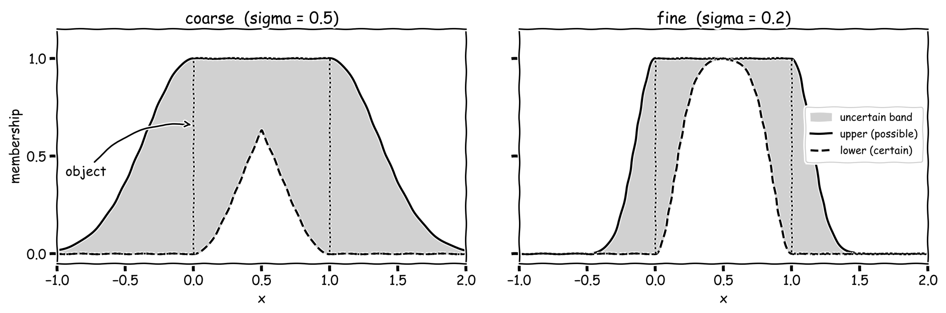
The fuzzy aura construction has a direct reading in multi-resolution image and signal segmentation, and this is the setting in which the resolution parameter becomes concrete. Picture a one-dimensional signal whose foreground is the region $[0,1]$, observed through a scope function that plays the role of the imaging window: each point x takes in its surroundings through the Gaussian window ${\tilde{a}}_{\sigma }\left(x\right)\left(y\right)=e^{-{(x-y)}^2/{\sigma }^2}$, whose width $\sigma$ is the resolution of the observation. Under this reading the two approximation operators are the two natural segmentations of the foreground. The lower approximation is the certain core, the points whose whole window stays inside the foreground; the upper approximation is the possible region, the points whose window still meets it; and the boundary is the uncertain edge band lying between the two. Sharpening the resolution, that is decreasing $\sigma$, sharpens the segmentation, and Theorem 20 guarantees that the edge band can only shrink, never grow. In morphological terms the upper and lower approximations are the fuzzy dilation and fuzzy erosion of the foreground by the structuring element ${\tilde{a}}_{\sigma }$, and the link between rough approximations and mathematical morphology is classical [50]; what the aura framework contributes is the topological reading of the same operators and the monotonicity guarantee.

• Setting.

Let $(\mathbb{R},{\tilde{\tau }}_u)$ be the real line with the triangular-neighborhood fuzzy topology of Example 2, and let ${\tilde{a}}_{\sigma }$ be the Gaussian aura of Example 4,

$${\tilde{a}}_{\sigma }\left(x\right)\left(y\right)=exp\left(-{\displaystyle \frac{{(x-y)}^2}{{\sigma }^2}}\right),x,y\in \mathbb{R},$$

for $\sigma >0$. The scope axiom ${\tilde{a}}_{\sigma }\left(x\right)\left(x\right)=1$ holds trivially, and ${\tilde{a}}_{\sigma }\left(x\right)\in {\tilde{\tau }}_u$ by Remark 2. The parameter $\sigma$ sets how widely a point x takes in its surroundings: small $\sigma$ confines attention to a thin neighborhood, while large $\sigma$ spreads it broadly.

• The foreground.

Take the foreground to be the unit interval, $\mu ={\chi }_{[0,1]}$, a crisp object sitting inside the fuzzy framework.

• Closed-form approximations.

A direct computation gives the upper approximation

$${\overline{\mathrm{apr}}}_{{\tilde{a}}_{\sigma }}\left(\mu \right)\left(x\right)=\underset{y\in [0,1]}{sup}exp\left(-{\displaystyle \frac{{(x-y)}^2}{{\sigma }^2}}\right)=\left\{\begin{array}{cc}exp(-x^2/{\sigma }^2),\hfill & x\le 0,\hfill \\ 1,\hfill & 0\le x\le 1,\hfill \\ exp(-{(x-1)}^2/{\sigma }^2),\hfill & x\ge 1,\hfill \end{array}\right.$$

and the lower approximation

$${\underline{\mathrm{apr}}}_{{\tilde{a}}_{\sigma }}\left(\mu \right)\left(x\right)=\underset{y\in \mathbb{R}}{inf}max\left\{1-exp\left(-{\displaystyle \frac{{(x-y)}^2}{{\sigma }^2}}\right),{\chi }_{[0,1]}\left(y\right)\right\}=\left\{\begin{array}{cc}1-exp\left(-{\displaystyle \frac{d{\left(x\right)}^2}{{\sigma }^2}}\right),\hfill & 0<x<1,\hfill \\ 0,\hfill & \mathrm{otherwise},\hfill \end{array}\right.$$

where $d\left(x\right)=min\{x,1-x\}$ is the distance from x to the boundary of $[0,1]$. The boundary function ${\mathrm{bnd}}_{{\tilde{a}}_{\sigma }}\left(\mu \right)\left(x\right)={\overline{\mathrm{apr}}}_{{\tilde{a}}_{\sigma }}\left(\mu \right)\left(x\right)-{\underline{\mathrm{apr}}}_{{\tilde{a}}_{\sigma }}\left(\mu \right)\left(x\right)$ thus takes a clean closed form on each region.

• Numerical sample (refinement).

Table 2 compares two scales ${\sigma }_1=0.5$ and ${\sigma }_2=0.2$ at several points of the real line.

Table 2. Upper approximation, lower approximation, and boundary of the foreground $\mu ={\chi }_{[0,1]}$ at the coarse scale ${\sigma }_1=0.5$ and the fine scale ${\sigma }_2=0.2$.

x	${\overline{\mathbf{apr}}}_{{\tilde{\mathit{a}}}_{{\mathit{\sigma }}_1}}$	${\underline{\mathbf{apr}}}_{{\tilde{\mathit{a}}}_{{\mathit{\sigma }}_1}}$	${\mathbf{bnd}}_{{\tilde{\mathit{a}}}_{{\mathit{\sigma }}_1}}$	${\overline{\mathbf{apr}}}_{{\tilde{\mathit{a}}}_{{\mathit{\sigma }}_2}}$	${\underline{\mathbf{apr}}}_{{\tilde{\mathit{a}}}_{{\mathit{\sigma }}_2}}$	${\mathbf{bnd}}_{{\tilde{\mathit{a}}}_{{\mathit{\sigma }}_2}}$
$-0.5$	0.368	0.000	0.368	0.002	0.000	0.002
$0.25$	1.000	0.221	0.779	1.000	0.790	0.210
$0.50$	1.000	0.632	0.368	1.000	0.998	0.002
$0.75$	1.000	0.221	0.779	1.000	0.790	0.210
$1.50$	0.368	0.000	0.368	0.002	0.000	0.002

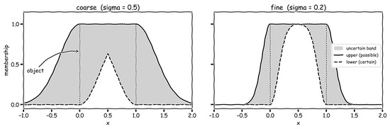
Figure 1 displays the two resolutions side by side. Since ${\sigma }_2<{\sigma }_1$ gives ${\tilde{a}}_{{\sigma }_2}\left(x\right)\left(y\right)\le {\tilde{a}}_{{\sigma }_1}\left(x\right)\left(y\right)$ pointwise, Theorem 20 predicts ${\underline{\mathrm{apr}}}_{{\tilde{a}}_{{\sigma }_1}}\le {\underline{\mathrm{apr}}}_{{\tilde{a}}_{{\sigma }_2}}$, ${\overline{\mathrm{apr}}}_{{\tilde{a}}_{{\sigma }_2}}\le {\overline{\mathrm{apr}}}_{{\tilde{a}}_{{\sigma }_1}}$, and ${\mathrm{bnd}}_{{\tilde{a}}_{{\sigma }_2}}\le {\mathrm{bnd}}_{{\tilde{a}}_{{\sigma }_1}}$. Reading the table in segmentation terms, the certain core grows and the uncertain band shrinks as the resolution sharpens from $\sigma =0.5$ to $\sigma =0.2$; all three inequalities can be read off directly.

Figure 1. Multi-resolution segmentation of the foreground $\mu ={\chi }_{[0,1]}$ through a Gaussian observation window. The certain core (lower), the possible region (upper), and the uncertain boundary band (shaded) are shown at a coarse resolution $\sigma =0.5$ and a fine resolution $\sigma =0.2$. As the resolution sharpens, the boundary band shrinks: its total area falls from $1.63$ to $0.71$, in line with the refinement monotonicity of Theorem 20. The dotted rectangle in each panel is the foreground $\mu$ itself, labelled “object” in the left panel.

• Asymptotic behavior.

The closed-form expressions yield clean limits. For any interior point $x\in (0,1)$ with $d\left(x\right)>0$,

$$\underset{\sigma \to 0^{+}}{lim}{\underline{\mathrm{apr}}}_{{\tilde{a}}_{\sigma }}\left(\mu \right)\left(x\right)=\underset{\sigma \to 0^{+}}{lim}\left(1-e^{-d{\left(x\right)}^2/{\sigma }^2}\right)=1,\underset{\sigma \to 0^{+}}{lim}{\mathrm{bnd}}_{{\tilde{a}}_{\sigma }}\left(\mu \right)\left(x\right)=0,$$

so as the window narrows, the two segmentations close in on the foreground itself: perfect resolution in the interior. In the opposite limit,

$$\underset{\sigma \to \infty }{lim}{\underline{\mathrm{apr}}}_{{\tilde{a}}_{\sigma }}\left(\mu \right)\left(x\right)=0,\underset{\sigma \to \infty }{lim}{\overline{\mathrm{apr}}}_{{\tilde{a}}_{\sigma }}\left(\mu \right)\left(x\right)=1(\mathrm{for}\mathrm{any}x\in \mathbb{R}),$$

the trivial-aura behavior of Proposition 4: once the resolution is gone the boundary saturates everywhere and the segmentation tells us nothing.

• Locally varying resolution.

The same closed-form analysis goes through when $\sigma$ depends on the point, $\sigma =\sigma \left(x\right)$ varying along $\mathbb{R}$. This is exactly the locally adaptive resolution one wants in practice, where a segmentation is allowed to be sharp in some regions and coarse in others, and it is the continuous counterpart of the variable scope function from the crisp aura construction of [30].

• A two-dimensional foreground.

Nothing in the computation is tied to the line, and the planar case is the one an image carries. Let $({\mathbb{R}}^2,{\tilde{\tau }}_u^{\left(2\right)})$ be the plane with the fuzzy topology generated by the conical neighborhoods ${\lambda }_{c,\epsilon }\left(y\right)=max\{0,1-\parallel y-c\parallel /\epsilon \}$, and put ${\tilde{a}}_{\sigma }\left(x\right)\left(y\right)={exp(-\parallel x-y\parallel }^2/{\sigma }^2)$. The Lipschitz argument of Remark 2 uses only the metric and the generators, so it applies here word for word: ${\tilde{a}}_{\sigma }\left(x\right)\in {\tilde{\tau }}_u^{\left(2\right)}$, and ${\tilde{a}}_{\sigma }$ is a fuzzy scope function on the plane. Take the foreground to be the unit square $S={[0,1]}^2$ and $\mu ={\chi }_S$. Write $d(x,S)$ for the Euclidean distance from x to S and $d(x,S^c)$ for the distance from x to the complement of S. The two computations run exactly as on the line and give

$${\overline{\mathrm{apr}}}_{{\tilde{a}}_{\sigma }}\left(\mu \right)\left(x\right)=exp\left(-{\displaystyle \frac{d{(x,S)}^2}{{\sigma }^2}}\right),{\underline{\mathrm{apr}}}_{{\tilde{a}}_{\sigma }}\left(\mu \right)\left(x\right)=1-exp\left(-{\displaystyle \frac{d{(x,S^c)}^2}{{\sigma }^2}}\right),$$

the first because the window is a decreasing function of distance, so its supremum over S is taken at the point of S nearest to x; the second because the terms with $y\in S$ contribute 1 to the infimum in (5) while those with $y\notin S$ contribute $1-exp(-\parallel x-y{\parallel }^2/{\sigma }^2)$, and among the latter the nearest point outside S decides. For x in the interior of S one has $d(x,S^c)=min\{x_1,1-x_1,x_2,1-x_2\}$, and ${\underline{\mathrm{apr}}}_{{\tilde{a}}_{\sigma }}\left(\mu \right)\left(x\right)=0$ for every other x.

Table 3 reads like Table 2, and the three inequalities of Theorem 20 can again be checked row by row. What the plane adds is the corner. Outside the square, the diagonal point $(-0.5,-0.5)$ already has a much weaker possible-region value than the side point $(-0.5,0.5)$, because its distance to S is larger by a factor $\sqrt{2}$; inside, the near-corner point $(0.1,0.1)$ keeps a wide boundary value even at the fine scale, where the point $(0.25,0.5)$ near the middle of an edge has largely resolved. Corners therefore sharpen later than edges as $\sigma$ decreases, which is the behavior one expects from erosion and dilation by a radially symmetric structuring element and which here falls straight out of the closed forms.

Table 3. The planar analogue of Table 2: approximations of the square foreground $\mu ={\chi }_{{[0,1]}^2}$ at the coarse scale ${\sigma }_1=0.5$ and the fine scale ${\sigma }_2=0.2$.

x	${\overline{\mathbf{apr}}}_{{\tilde{\mathit{a}}}_{{\mathit{\sigma }}_1}}$	${\underline{\mathbf{apr}}}_{{\tilde{\mathit{a}}}_{{\mathit{\sigma }}_1}}$	${\mathbf{bnd}}_{{\tilde{\mathit{a}}}_{{\mathit{\sigma }}_1}}$	${\overline{\mathbf{apr}}}_{{\tilde{\mathit{a}}}_{{\mathit{\sigma }}_2}}$	${\underline{\mathbf{apr}}}_{{\tilde{\mathit{a}}}_{{\mathit{\sigma }}_2}}$	${\mathbf{bnd}}_{{\tilde{\mathit{a}}}_{{\mathit{\sigma }}_2}}$
$(-0.5,-0.5)$	0.135	0.000	0.135	0.000	0.000	0.000
$(-0.5,0.5)$	0.368	0.000	0.368	0.002	0.000	0.002
$(0.1,0.1)$	1.000	0.039	0.961	1.000	0.221	0.779
$(0.25,0.5)$	1.000	0.221	0.779	1.000	0.790	0.210
$(0.5,0.5)$	1.000	0.632	0.368	1.000	0.998	0.002

• What these examples do and do not show.

Both computations are illustrations of the theory rather than an empirical validation of a segmentation method. There is no real image or benchmark dataset here, and no comparison against existing fuzzy or rough segmentation algorithms. What they do is exhibit the two operators in closed form, make the resolution parameter visible, and confirm the qualitative content of Theorem 20 in cases where every quantity can be computed by hand. An experimental study on real data, with such a comparison, is a separate undertaking and we have not attempted it here; Section 9 returns to this point.

8. Comparison with Existing Fuzzy Auxiliary Structures

Where does the fuzzy aura sit among the other auxiliary structures on a fuzzy topological space? Table 4 lines it up against fuzzy ideals, fuzzy grills, and the Dubois–Prade fuzzy rough set model; the crisp version of this comparison appears in Section 7 of [30]. By Remark 4 the aura and Dubois–Prade columns share their operators, so the differences lie in the data carried and in the interaction with $\tilde{\tau }$. The correspondence between reflexive transitive fuzzy relations and fuzzy topologies is itself classical [33,34]; the aura sits on the non-transitive side of it, where the closure is genuinely Čech.

Table 4. How the fuzzy aura compares with the other auxiliary structures on a fuzzy topological space $(X,\tilde{\tau })$.

	Fuzzy Ideal $\tilde{\mathcal{I}}$	Fuzzy Grill $\tilde{\mathcal{G}}$	Dubois–Prade	Fuzzy Aura $\tilde{\mathit{a}}$
Auxiliary datum	a subfamily of $I^X$	a subfamily of $I^X$	a reflexive fuzzy relation R	a reflexive fuzzy relation with fuzzy-open foresets, $\tilde{a}:X\to \tilde{\tau }$
Induced closure	Kuratowski	Kuratowski	Čech in general, Kuratowski when R is transitive	the same operators as Dubois–Prade
Interaction with $\tilde{\tau }$	refines it	refines it	none required	scope values must be fuzzy open; ${\tilde{\tau }}_{\tilde{a}}$ in general not comparable with $\tilde{\tau }$
Mixed operators with the ambient interior	no	no	no	yes: five classes of generalized open sets (Section 4)

The main point the table makes is that the aura is not lighter data than a relation; it is a reflexive fuzzy relation, packaged per point, with the additional compatibility requirement that each foreset be fuzzy open. That requirement is precisely what lets the aura interact with the ambient topology: the mixed operators of Section 4 compose the ambient interior with the aura closure, and no purely relational or ideal-theoretic construction produces the resulting hierarchy or its failures (Remark 12). There is also a contrast of direction: where an ideal or a grill refines $\tilde{\tau }$, the aura replaces it. Under the trivial aura the induced ${\tilde{\tau }}_{\tilde{a}}$ can even collapse to the constants (Proposition 4), erasing every separation property of the ambient space, which is something a refining construction can never force. The closure itself is only Čech in general (Theorem 3) and turns Kuratowski when $\tilde{a}$ is transitive (Theorem 7); by Proposition 3, iterating it never produces a topology beyond ${\tilde{\tau }}_{\tilde{a}}$ itself.

The table compresses several distinct relationships into one column, so it is worth walking through the neighboring frameworks one at a time; the aura stands at a different distance from each.

Fuzzy relations without reflexivity. Formulas (2) and (4) make sense for any fuzzy relation, but the scope axiom $\tilde{a}\left(x\right)\left(x\right)=1$ is exactly reflexivity, and it is what delivers extensivity of ${\mathrm{cl}}_{\tilde{a}}$ and contractivity of ${\mathrm{int}}_{\tilde{a}}$ (Theorem 1(b), Theorem 4(b)). Drop it and the pair is no longer a closure–interior pair at all, so nothing topological survives; every result in this paper uses reflexivity from the first line.

Reflexive fuzzy relations. Here the relationship is an equality rather than a specialization: by Remark 4 the aura operators are the Dubois–Prade operators of $R(x,y)=\tilde{a}\left(x\right)\left(y\right)$, and conversely every reflexive fuzzy relation whose foresets $R(x,·)$ are fuzzy open is a scope function (Remark 19(ii)). In data, therefore, the aura is a restricted relation; in statements it is the wider setting, because the ambient topology can be quantified over. Proposition 8, which decides from $\tilde{\tau }$ alone whether any separating scope function exists at all, and Theorem 18, which fixes $\tilde{\tau }$ and varies $\tilde{a}$, are both of this kind and have no formulation on the purely relational side.

Fuzzy neighborhood operators. A scope function is a fuzzy neighborhood operator in the sense used for covering-based fuzzy rough sets by D’eer, Cornelis, and Godo [35]: it assigns one fuzzy set to each point, and the induced approximations are the usual ones. Two differences are worth naming. Their neighborhoods are derived from a covering and inherit whatever regularity the covering has, whereas ours are prescribed directly and are constrained only by fuzzy openness; and the generalized open sets of Section 4 pair the neighborhood-induced closure with the ambient interior, a combination that does not arise when the topology is absent (Remark 10).

Fuzzy rough sets. As a model of graded indiscernibility, the aura pair is the Dubois–Prade model [26]; the comparative account of Radzikowska and Kerre [27], the constructive and axiomatic theory of Yao [28], Morsi and Yakout [31], and Wu, Mi, and Zhang [32], all apply to it unchanged. When $\tilde{a}$ is symmetric and transitive we are in the fuzzy equivalence case of the classical model (Theorem 8), and the refinement statement of Theorem 20 is the comparison across granulations that multigranulation models exploit [49]. What the aura contributes is not a new approximation model but a topological environment for an existing one.

Fuzzy closure spaces. By Theorem 1 the pair $(X,{\mathrm{cl}}_{\tilde{a}})$ is a fuzzy closure space in the sense of Mashhour and Ghanim [43], and by Theorem 6 its iteration is Kuratowski. The aura ones form a proper subclass: ${\mathrm{cl}}_{\tilde{a}}$ is completely additive (Lemma 2), which a fuzzy Čech closure need not be, and it is determined by its values on the crisp points, since ${\mathrm{cl}}_{\tilde{a}}\left({\chi }_{\left\{y\right\}}\right)\left(x\right)=\tilde{a}\left(x\right)\left(y\right)$ and complete additivity recovers ${\mathrm{cl}}_{\tilde{a}}\left(\mu \right)$ from these. Its provenance is what a general fuzzy closure space lacks, and it is what makes the scale-additivity law of Proposition 6 and the achievability criterion of Proposition 8 expressible at all.

9. Conclusions

We introduced fuzzy aura topological spaces $(X,\tilde{\tau },\tilde{a})$, generalizing the crisp aura spaces to the fuzzy setting. The central operator is the fuzzy aura-closure ${\mathrm{cl}}_{\tilde{a}}$, a fuzzy additive Čech closure that is not idempotent in general; we gave a counterexample and showed it becomes idempotent once $\tilde{a}$ is transitive. Its iteration is a Kuratowski closure with the same fixed points, so the derived fuzzy aura topology ${\tilde{\tau }}_{\tilde{a}}$ is unambiguous; unlike in the crisp theory, it need not be contained in the ambient topology, as a two-point example shows. From ${\mathrm{cl}}_{\tilde{a}}$ and its dual interior we built five classes of generalized fuzzy open sets and placed them in a hierarchy, with counterexamples on finite spaces and on the real line showing each inclusion to be strict. On the real line the closure obeys a scale-additivity law: it maps triangular and Gaussian profiles to profiles of the same family with the widths added (Proposition 6), so the aura closure of these fuzzy open profiles stays fuzzy open.

We then studied fuzzy $\tilde{a}$-continuity, proving decomposition theorems and in particular the identity $\tilde{a}$-$F\alpha O=\tilde{a}$-$\mathrm{FSO}\cap \tilde{a}$-$\mathrm{FPO}$ under transitivity (Corollary 1). The separation axioms fuzzy $\tilde{a}$-$T_i$ ($i=0,1,2$) and fuzzy $\tilde{a}$-regularity were tied to the scope function: distinctness of the auras is necessary for fuzzy $\tilde{a}$-$T_0$ though not sufficient, fuzzy $\tilde{a}$-$T_1$ is characterized completely by the vanishing of the cross-auras, and the discrete crisp aura forces both fuzzy $\tilde{a}$-$T_2$ and fuzzy $\tilde{a}$-regularity; separation thus rests on the auras and not on the ambient topology. In fact the ungraded $T_1$ and $T_2$ axioms collapse: they are equivalent to each other and to the aura being discrete and crisp (Corollary 3), and a space admits such a scope function precisely when its crisp singletons are fuzzy open (Proposition 8). The graded, level-indexed variant of $T_1$ restores nontrivial content for continuous auras; the sampled Gaussian aura, for instance, is separated exactly above the level $e^{-{\delta }^2/{\sigma }^2}$ set by the sampling step and the window width. The rough approximation operators coincide with the Dubois–Prade pair of the associated reflexive fuzzy relation and recover the Pawlak and crisp aura models as special cases, and the refinement monotonicity theorem turns the scope width into a resolution parameter, with finer auras giving tighter approximations and smaller boundaries. Section 7 reads that statement as multi-resolution segmentation.

Two limitations should be stated plainly. The first concerns novelty: the approximation operators themselves are the Dubois–Prade operators of a reflexive fuzzy relation, and every result about them alone belongs to the existing relational theory. What we claim as new lives in the interaction between the scope function and the ambient topology, and the reader can locate it precisely: the hierarchy of the five mixed classes and its strictness, the failure of the Njåstad property and what that failure costs (Remark 13), the scale-additivity law, the collapse of the ungraded separation axioms with the criterion for admitting a separating scope function, and the graded level-$\alpha$ axiom. The second concerns the segmentation reading of Section 7. The one- and two-dimensional computations there are illustrations, not experiments: they involve no real image or benchmark data and no comparison with existing segmentation methods, and they should be read as showing what the operators look like at two resolutions rather than as evidence of practical performance. Testing the construction on real data, against the standard fuzzy and rough alternatives, is the obvious next step and is not undertaken here.

A few questions are left open. In the crisp theory the containment ${\tau }_a\subseteq \tau$ makes aura-compactness easier to reach than ordinary compactness; in the fuzzy setting this containment can fail, so even the correct comparison between aura-compactness and fuzzy compactness is unsettled. We have not pursued it here, though the recent treatment of compactness via primal structures [10] suggests one route. Products and subspaces are also untreated, and it is not clear when refinement monotonicity survives them. One could also combine the scope function and a fuzzy ideal in a single local function, which would sit between the aura-closure ${\mathrm{cl}}_{\tilde{a}}$ and the ideal-closure ${\mathrm{cl}}^{*}$ and tie together two structures that have each been studied at length [24,25].

References

- Kuratowski, K. Topologie I; Monografje Matematyczne: Warsaw, Poland, 1933. [Google Scholar]
- Vaidyanathaswamy, R. The localisation theory in set-topology. Proc. Indian Acad. Sci. 1945, 20, 51–61. [Google Scholar] [CrossRef] [Scilit]
- Janković, D.; Hamlett, T.R. New topologies from old via ideals. Am. Math. Mon. 1990, 97, 295–310. [Google Scholar] [CrossRef] [Scilit]
- Cartan, H. Théorie des filtres. C. R. Acad. Sci. Paris 1937, 205, 595–598. [Google Scholar]
- Choquet, G. Sur les notions de filtre et de grille. C. R. Acad. Sci. Paris 1947, 224, 171–173. [Google Scholar]
- Roy, B.; Mukherjee, M.N. On a typical topology induced by a grill. Soochow J. Math. 2007, 33, 771–786. [Google Scholar]
- Al-Omari, A.; Noiri, T. On ΨG-sets in grill topological spaces. Filomat 2011, 25, 187–196. [Google Scholar] [CrossRef] [Scilit]
- Acharjee, S.; Özkoç, M.; Issaka, F.Y. Primal topological spaces. Bol. Soc. Parana. Mat. 2025, 43, 1–9. [Google Scholar] [CrossRef] [Scilit]
- Al-Omari, A.; Alqahtani, M.H. Primal structure with closure operators and their applications. Mathematics 2023, 11, 4946. [Google Scholar] [CrossRef] [Scilit]
- Alghamdi, O. On the compactness via primal topological spaces. AIMS Math. 2024, 9, 32124–32137. [Google Scholar] [CrossRef] [Scilit]
- Zadeh, L.A. Fuzzy sets. Inf. Control 1965, 8, 338–353. [Google Scholar] [CrossRef] [Scilit]
- Chang, C.L. Fuzzy topological spaces. J. Math. Anal. Appl. 1968, 24, 182–190. [Google Scholar] [CrossRef] [Scilit]
- Lowen, R. Fuzzy topological spaces and fuzzy compactness. J. Math. Anal. Appl. 1976, 56, 621–633. [Google Scholar] [CrossRef] [Scilit]
- Molodtsov, D. Soft set theory—First results. Comput. Math. Appl. 1999, 37, 19–31. [Google Scholar] [CrossRef] [Scilit]
- Shabir, M.; Naz, M. On soft topological spaces. Comput. Math. Appl. 2011, 61, 1786–1799. [Google Scholar] [CrossRef] [Scilit]
- Pawlak, Z. Rough sets. Int. J. Comput. Inf. Sci. 1982, 11, 341–356. [Google Scholar] [CrossRef] [Scilit]
- El-Bably, M.K.; Fleifel, K.K.; Embaby, O.A. Topological approaches to rough approximations based on closure operators. Granul. Comput. 2022, 7, 1–14. [Google Scholar] [CrossRef] [Scilit]
- Lin, E.-B. Categorical structures in rough set theory and information systems. Mathematics 2026, 14, 369. [Google Scholar] [CrossRef] [Scilit]
- Zhan, J.; Alcantud, J.C.R. A novel type of soft rough covering and its application to multicriteria group decision making. Artif. Intell. Rev. 2019, 52, 2381–2410. [Google Scholar] [CrossRef] [Scilit]
- Al-shami, T.M.; Hosny, R.A.; Mhemdi, A.; Hosny, M. Cardinality rough neighborhoods with applications. AIMS Math. 2024, 9, 31366–31392. [Google Scholar] [CrossRef] [Scilit]
- Mareay, R.; Abu-Gdairi, R.; Badr, M. Soft rough fuzzy sets based on covering. AIMS Math. 2024, 9, 11180–11193. [Google Scholar] [CrossRef] [Scilit]
- Wang, R.; Xie, X.; Zhi, H. Bi-fuzzy S-approximation spaces. Mathematics 2025, 13, 324. [Google Scholar] [CrossRef] [Scilit]
- Swaminathan, A.; Sheela, M. Applications of fuzzy maximal μ-open sets in generalized fuzzy topology and fuzzy quasi topology. Bol. Soc. Parana. Mat. 2026, 44, 1–5. [Google Scholar]
- Abbas, F. Fuzzy ideal supra topological spaces. Adv. Fuzzy Syst. 2020, 2020, 8824296. [Google Scholar] [CrossRef] [Scilit]
- Açıkgöz, A. New fuzzy topologies via ideals and generalized openness. Mathematics 2026, 14, 904. [Google Scholar] [CrossRef] [Scilit]
- Dubois, D.; Prade, H. Rough fuzzy sets and fuzzy rough sets. Int. J. Gen. Syst. 1990, 17, 191–209. [Google Scholar] [CrossRef] [Scilit]
- Radzikowska, A.M.; Kerre, E.E. A comparative study of fuzzy rough sets. Fuzzy Sets Syst. 2002, 126, 137–155. [Google Scholar] [CrossRef] [Scilit]
- Yao, Y.Y. Constructive and algebraic methods of the theory of rough sets. Inf. Sci. 1998, 109, 21–47. [Google Scholar] [CrossRef] [Scilit]
- Chacón-Gómez, F.; Cornejo, M.E.; Medina, J. Decision making in fuzzy rough set theory. Mathematics 2023, 11, 4187. [Google Scholar] [CrossRef] [Scilit]
- Açıkgöz, A. Generalized open sets and closure operators via point-to-neighborhood assignments. Mathematics 2026, 14, 1013. [Google Scholar] [CrossRef] [Scilit]
- Morsi, N.N.; Yakout, M.M. Axiomatics for fuzzy rough sets. Fuzzy Sets Syst. 1998, 100, 327–342. [Google Scholar] [CrossRef] [Scilit]
- Wu, W.-Z.; Mi, J.-S.; Zhang, W.-X. Generalized fuzzy rough sets. Inf. Sci. 2003, 151, 263–282. [Google Scholar] [CrossRef] [Scilit]
- Qin, K.; Pei, Z. On the topological properties of fuzzy rough sets. Fuzzy Sets Syst. 2005, 151, 601–613. [Google Scholar] [CrossRef] [Scilit]
- Lai, H.; Zhang, D. Fuzzy preorder and fuzzy topology. Fuzzy Sets Syst. 2006, 157, 1865–1885. [Google Scholar] [CrossRef] [Scilit]
- D’eer, L.; Cornelis, C.; Godo, L. Fuzzy neighborhood operators based on fuzzy coverings. Fuzzy Sets Syst. 2017, 312, 17–35. [Google Scholar] [CrossRef] [Scilit]
- Azad, K.K. On fuzzy semicontinuity, fuzzy almost continuity and fuzzy weakly continuity. J. Math. Anal. Appl. 1981, 82, 14–32. [Google Scholar] [CrossRef] [Scilit]
- Bin Shahna, A.S. On fuzzy strong semicontinuity and fuzzy precontinuity. Fuzzy Sets Syst. 1991, 44, 303–308. [Google Scholar] [CrossRef] [Scilit]
- Thakur, S.S.; Singh, S. On fuzzy semi-preopen sets and fuzzy semi-precontinuity. Fuzzy Sets Syst. 1998, 98, 383–391. [Google Scholar] [CrossRef] [Scilit]
- Levine, N. Semi-open sets and semi-continuity in topological spaces. Am. Math. Mon. 1963, 70, 36–41. [Google Scholar] [CrossRef] [Scilit]
- Njåstad, O. On some classes of nearly open sets. Pac. J. Math. 1965, 15, 961–970. [Google Scholar] [CrossRef] [Scilit]
- Mashhour, A.S.; Ghanim, M.H.; Fath Alla, M.A. On fuzzy non-continuous mappings. Bull. Calcutta Math. Soc. 1986, 78, 57–69. [Google Scholar]
- Čech, E. Topological Spaces; Wiley: London, UK, 1966. [Google Scholar]
- Mashhour, A.S.; Ghanim, M.H. Fuzzy closure spaces. J. Math. Anal. Appl. 1985, 106, 154–170. [Google Scholar] [CrossRef] [Scilit]
- Andrijević, D. On b-open sets. Mat. Vesn. 1996, 48, 59–64. [Google Scholar]
- Benchalli, S.S.; Karnel, J.J. On fuzzy b-open sets in fuzzy topological spaces. J. Comput. Math. Sci. 2010, 1, 127–134. [Google Scholar] [CrossRef] [Scilit]
- Lindeberg, T. Scale-Space Theory in Computer Vision; Kluwer Academic Publishers: Dordrecht, The Netherlands, 1994. [Google Scholar]
- Dubois, D.; Prade, H. Operations on fuzzy numbers. Int. J. Syst. Sci. 1978, 9, 613–626. [Google Scholar] [CrossRef] [Scilit]
- Saleh, S.; Al-shami, T.M.; Azzam, A.A.; Hosny, M. Stronger forms of fuzzy pre-separation and regularity axioms via fuzzy topology. Mathematics 2023, 11, 4801. [Google Scholar] [CrossRef] [Scilit]
- Qian, Y.; Liang, J.; Yao, Y.; Dang, C. MGRS: A multi-granulation rough set. Inf. Sci. 2010, 180, 949–970. [Google Scholar] [CrossRef] [Scilit]
- Bloch, I. On links between mathematical morphology and rough sets. Pattern Recognit. 2000, 33, 1487–1496. [Google Scholar] [CrossRef] [Scilit]
Disclaimer/Publisher’s Note: The statements, opinions and data contained in all publications are solely those of the individual author(s) and contributor(s) and not of MDPI and/or the editor(s). MDPI and/or the editor(s) disclaim responsibility for any injury to people or property resulting from any ideas, methods, instructions or products referred to in the content. |
© 2026 by the authors. Licensee MDPI, Basel, Switzerland. This article is an open access article distributed under the terms and conditions of the Creative Commons Attribution (CC BY) license.