


Abstract
One of the most important parameters in fetal monitoring is the fetal heart rate (fHR). However, due to the nature of this signal, several non-invasive techniques have been developed for fetal monitoring, including Cardiotocography (CTG), Doppler Echocardiography (Doppler Echo), fetal electrocardiography (fECG), fetal phonocardiography (fPCG), fetal Magnetocardiography (fMCG), and fetal Photoplethysmography (fPPG). Fetal phonocardiography is a passive, safe, and non-invasive method for estimating fHR, in which an acoustic signal is acquired through a transducer placed on the mother’s abdomen to capture sounds associated with fetal cardiac activity. In this paper, we propose a hybrid framework for fHR estimation that integrates digital signal processing techniques with a deep learning approach. The method employs a Hermite Transform (HT)-based bio-inspired vision model for fPCG signal denoising, the Hilbert transform to extract the signal envelope, and Mel-Frequency Cepstral Coefficients (MFCCs) to generate spectrogram-based features. Then, these features, represented as image-like, are used to train and evaluate a hybrid architecture that synergistically combines convolutional neural networks (CNNs) with Bidirectional Long Short-Term Memory (BiLSTM). BiLSTM is a deep learning model that processes sequential information in both forward and backward directions, thereby extending the memory capabilities of conventional Recurrent Neural Networks (RNNs). Thus, CNNs are used to capture intricate spatial morphologies of the fPCG signals, whereas BiLSTM captures their temporal evolution across consecutive time windows. Additionally, to assess its generalization capability, the proposed method is evaluated on two publicly available fPCG datasets and benchmarked against several state-of-the-art approaches. The experimental results demonstrate that the proposed method achieves competitive performance across different datasets, highlighting its effectiveness and robustness.
Keywords:
fetal heart sounds; fPCG; fHR; deep learning; MFCCs; image-like; spectrogram-based; Hermite Transform; BiLSTM; CNNs; fetal health MSC:
92C55; 68U10; 68T05
1. Introduction
The 2030 Agenda, published by the United Nations in 2015, aims to improve the lives of people worldwide. Therefore, they proposed 17 objectives related to sustainable development [1]. One of them is focused on health and well-being, with the key objective of reducing neonatal mortality to at least 12 per 1000 live births. To prevent this mortality, monitoring of the fetus during pregnancy is recommended. So, the mother must have periodic check-ups to monitor her health, but above all, the growth of the fetus. Nowadays, medical personnel can utilize various non-invasive techniques to monitor fetal growth, enabling them to assess different factors that help determine whether the fetus is developing optimally. These techniques are CTG, Doppler Echo, fECG, fPCG, fMCG, and fPPG [2]. Therefore, when evaluating fetal health, it is necessary to measure heart sounds, because this allows the doctor to recommend the most suitable treatment or refer the pregnant woman to a specialist. In developing countries, the minimum options available to assess fetal growth and, above all, provide timely warnings if a pregnancy presents any abnormalities are still unclear. Therefore, the need for affordable and accessible alternatives in medical equipment, such as ultrasound, is clear, not only for poor regions and those far from large cities, but in general, for providing maternal and fetal care during pregnancy. A simple option is the acquisition and analysis of phonocardiography signals, which can be obtained by placing a microphone on the pregnant woman’s abdomen and performing the test under the supervision of a general practitioner at a local medical center. fPCG is a graphic recording of fetal heart activity and is measured on the surface of the mother’s body. It allows one to evaluate fetal well-being, estimate the fetal heart rate, and detect heart problems. The microphone is used for its portability, passive operation, and energy-free operation. One of the main advantages is that the microphone does not produce thermal effects that can damage the fetus in prolonged exposures [2,3]. However, one of the main problems with fPCG signals is noise, as signals can be distorted by artifacts from surrounding maternal organs and tissues, body movement, respiratory activity, and uterine contractions. However, fPCG-based monitoring could become a competitive alternative to electronic fetal monitoring if both signal acquisition and processing are improved.
In a fetus, the heart sounds S1 and S2 are detectable and fall within the audible range of 20 to 200 Hz, while a fetus’s heart rate ranges between 120 and 180 Beats Per Minute (BPM). Measurement of heart rate and the central frequencies of the S1 and S2 sounds, along with their respective bandwidths, enables the evaluation of the fetal cardiac condition. Different proposals have been developed that focus on this type of signal or focus on methods for extracting the phonocardiography signal [4]. In [4], the authors emphasized the importance of phonocardiography and provided techniques to analyze phonocardiography signals, as well as an analysis of the Wavelet Transform (WT) to prepare the fPCG signal. Some research focuses on evaluating and describing trends, challenges, and future directions in fetal monitoring. Also, some methods have focused on the limitations of modern and traditional monitoring techniques, such as fPCG. Ref. [5] presents different techniques for measuring fetal Heart Rate (fHR), including fPCG. Also, the authors explain that textile-based wearable technology for fHR monitoring could improve fetal heart surveillance through continuous data collection and ergonomic design. In addition, some papers discuss hardware, specifically acquisition devices for fPCG. In [6], the authors focused on monitoring devices (performance and design). They identified 24 devices that use four technologies: fetal electrocardiography, fetal phonocardiography, accelerometry, and fetal vectorcardiography. Finally, other techniques considered include machine learning, deep learning, and artificial neural networks. On the one hand, machine learning can automate the analysis of fPCG recordings, be trained on large datasets of labeled fPCG recordings, or handle large volumes of data [7]. On the other hand, artificial intelligence can be used to diagnose congenital heart disease. The paper [8] presents the use of artificial intelligence to diagnose congenital heart disease. Also, the authors indicate the relevance of intelligence in predicting some types of lesions and the importance of more research with larger populations to provide sufficient statistical data.
Several challenges must be considered when processing fPCG signals. For instance, this type of signal is highly noisy and contains frequency components unrelated to the fetal heartbeat. Therefore, denoising, filtering, and signal enhancement techniques are necessary to isolate and extract the signal of interest.
In this paper, we propose a hybrid fHR estimation approach that employs the Hermite Transform (HT)-based bio-inspired vision model for fPCG signal denoising, providing an alternative to conventional wavelet-based denoising methods. Additionally, the Hilbert transform envelope and spectrogram features are extracted from the fPCG signals and mapped via MFCCs to construct image representations of the 1D fPCG signals. These feature images are then used as inputs to a BiLSTM configured for fHR estimation as a regression task. For evaluation, the proposed hybrid fHR estimation method is tested on two fPCG datasets acquired under real-world conditions. The first dataset, SUFHSDB [9], consists of 104 fPCG recordings from four twin pregnancies, with durations ranging from 30 s to 90 s. This dataset also provides reference fHR values computed over 10 s windows. The second dataset, IIScFHSDB [10,11], was collected from 47 pregnant women, with an average recording duration of approximately 8 min. This dataset provides only a single reference fHR value per complete recording; therefore, it is used exclusively for testing. Experimental evaluation demonstrates the effectiveness of the proposed approach, achieving competitive performance compared to several state-of-the-art fHR estimation methods. The main contributions of this work are summarized as follows:
- Hermite transform-based fPCG signal denoising: To the best of our knowledge, this is the first time that the Hermite transform has been used for denoising the fPCG signals, which is an alternative to conventional wavelet-based denoising methods.
- Spectrogram-based Mel-Frequency Cepstral Coefficients feature extraction for BiLSTM-driven fHR estimation: To the best of our knowledge, the spectrogram-based MFCCs feature extraction coupled with BiLSTM regression has not previously been applied to fHR estimation.
- Image-like feature representations: Instead of processing the fPCG signals as 1D representations, this work extracts spectrogram-based MFCCs to generate image-like feature maps that serve as inputs for 2D CNNs and BiLSTM architectures.
- fHR estimation evaluation using real-world fPCG datasets: The proposed fHR estimation method was trained on a dataset acquired under realistic conditions rather than on simulated-signal datasets. Additionally, the trained network was evaluated on a dataset with limited fHR reference annotations, achieving competitive results.
The remainder of the paper is organized as follows. Section 2 presents a review of recent studies on fHR estimation using fPCG signals. Section 3 briefly describes the available datasets for studying and testing fPCG signals, remarking the importance of this topic because there are not enough datasets, so some researchers have made their own synthetic signals. Next, we present the methods and mathematical foundations underlying the proposed hybrid fHR estimation method. Section 4 details the proposed fHR estimation method, which combines an HT-based bio-inspired vision model for fPCG signal denoising with Mel-Frequency Cepstral Coefficients for spectrogram feature representation. A BiLSTM network then uses these features to perform a regression task and estimate fHR. Section 5 presents the experimental setup, the evaluation metrics, the results obtained by applying the proposed hybrid fHR estimation method to the two public fPCG datasets, and a comparison with several state-of-the-art approaches. Finally, Section 6 and Section 7 present the discussion of the results and the conclusions of the study, respectively.
2. Related Work
As we mentioned, processing fPCG signals poses several challenges due to their high noise levels, so various techniques have been proposed to denoise and filter them to isolate and extract the signal of interest. We first provide a brief description of different techniques, dividing them into denoising, filtering, and signal enhancement and then present some approaches for HR estimation.
2.1. Denoising Fetal Phonocardiogram Signals
The first characteristic of the fPCG signals is their nonstationary nature and relatively small amplitudes, which make them highly sensitive to noise during acquisition. Among the most common sources of interference are environmental noise with frequency components around 10 Hz, as well as maternal speech or coughing during the acquisition process [12].
Given this nonstationary characteristic, one widely used technique for removing noise from fPCG signals is the WT [13,14,15,16]. For example, Sbrollini et al. [17] evaluated the WT’s ability and robustness to denoise fPCG characterized by varying signal-to-noise ratios (SNRs). The authors employed a fourth-order Coiflet mother wavelet with seven levels of decomposition, demonstrating that this was a suitable and robust technique for denoising fPCG signals, as it preserved the fundamental fPCG features. Suryani et al. [18] used a linear regression to determine the optimal decomposition of the Coiflet wavelet and evaluated the sqtwolog, minimaxi, and SURE thresholding algorithms. The authors concluded that the signal could be decomposed into six levels using Coiflet 3 wavelets. In [19], Minani and Malarvili identified the most appropriate parameters for a Discrete Wavelet Transform (DWT) decomposition to denoise the fPCG signal and the signal of the mother. According to their results, the authors concluded that the best performance for denoising both the fetal and maternal heart sounds could be achieved when combining db10 as the mother wavelet at the sixth level of decomposition. A different proposal is described in [20]. The authors used adaptive Support Vector Regression (SVR) to denoise fPCG signals. They indicated that, in that form, the clean fetal heart signals extracted from the interfered source could be further used to generate the fPCG and calculate the fHR.
On the other hand, a popular denoising approach has been Empirical Mode Decomposition (EMD). For example, Vadali et al. [21] applied EMD to denoise and extract both fetal and maternal signals. The authors demonstrated that the bandwidths of extracted FHS and MHS signals were consistent with the existing gold standards. Cheikh et al. [22] proposed the Improved Complete Ensemble Empirical Mode Decomposition with Adaptive Noise (ICEEMDAN) method, which included wavelet transform thresholding and a metaheuristic search algorithm, indicating that their method had better suppression of mode mixing and a minimized number of Intrinsic Mode Functions (IMFs). Jatia and Veer [23] implemented and compared two denoising techniques: a Finite Impulse Response (FIR) filter method and an EMD approach. Pauline et al. [24] proposed the Variable Stage Cascaded Sign Error LMS (SELMS) adaptive filter model: a cascade of adaptive filters combined with the Sign Error LMS adaptation algorithm. According to the conclusions, their method offered an improved solution that achieved faster convergence and lower Mean Squared Error (MSE) by automatically adjusting the number of filter stages cascaded and the step size for each stage.
2.2. Filtering and Enhancement of Fetal Phonocardiogram Signals
Filtering is a common preprocessing step applied to fPCG signals. It is used for signal enhancement and for removing unwanted components present in the original fPCG signal. Some examples of unwanted components include artifacts caused by maternal and fetal motion, which generate random impulse noise (0–100 Hz) and reverberation noise (0–25 Hz). In addition, maternal heart sounds (10–40 Hz), uterine contractions, and maternal breathing (0.2–0.5 Hz) interact with the fPCG signal. Furthermore, artifacts may interfere with the fPCG signal, such as quantization noise from the transducer and sounds from maternal digestion [12]. Thus, in [25], the authors proposed an enhanced fPCG method using the WT and Hilbert transform to extract fetal heart sounds from the mixed signal, obtaining an overall performance of 90% in the correct localization of the fHS. Similarly, ref. [26] presented the Ensemble EMD (EEMD) as an fPCG enhancement approach; this method allows the analysis of heart sounds via IMFs and is adaptive and data-driven. In [27], Tomassini et al. evaluated several filtering approaches based on wavelet transforms; specifically, Coiflet, Daubechies, and Symlet wavelets were compared. Additionally, soft and hard thresholding rules, as well as the Universal, Rigorous, and Minimax thresholding algorithms, were tested. In [28], Strazza et al. used the Coiflet mother wavelet within a hierarchical decomposition strategy to determine the optimal thresholding rule for signal denoising. Martinek et al. [29] performed a study to evaluate how filtering fPCG signals using EMD, EEMD, and adaptive wavelet transform-based methods, under different types and levels of noise and degradation (e.g., Gaussian noise and motion artifacts from the fetus and mother), affected signal integrity.
In contrast, Zhdanov et al. [30] conducted a study to determine the optimal parameters for denoising highly noisy fPCG signals using wavelet-transform-based filtering. Daubechies, Coiflet, and Symlet wavelets were evaluated, and Maximal Overlap DWT (MODWT), Stein’s method, adaptive WT, and a heuristic approach were considered as denoising methods. In [12], Barnova et al. compared the Savitzky–Golay filter, Adaptive WT (AWT), EMD, EEMD, MODWT, FIR filters, and other filtering approaches using synthetic fPCG signals under multiple single and combined distortion scenarios, including maternal cardiac sounds, movement-related artifacts, Gaussian noise, and environmental noise. On the other hand, Kong et al. [31] applied an fPCG segmentation approach based on Transformer architectures and eXtreme Gradient Boosting (XGBoost) to determine fetal heart sounds. Additionally, the effects of various disturbances (maternal cardiac sounds, motion artifacts, and noise) on segmentation accuracy were evaluated. Bhaskaran and Arora [32] proposed algorithms for automatically selecting the filter frequency band based on signal characteristics for fetal heart sound processing within a framework that used Hilbert-autocorrelation and cyclic frequency repetition methods.
2.3. Fetal Heart Rate Estimation Methods
Regarding heart rate estimation methods based on fPCG signals, both single-channel and multi-channel approaches have been proposed. Single-channel methods pose a greater challenge due to the limited information available. Thus, Zhdanov et al. [33] used the normalized average Shannon energy of fPCG signals acquired with a piezoelectric sensor to extract heart sounds. First, an active fourth-order band-pass filter was applied to preprocess the signals; next, median filtering followed by an adaptive thresholding algorithm was used to calculate the fHR. Tang et al. [34] applied a Fourier series expansion to compute the cyclic frequency spectrum of the autocorrelation of the fPCG signals. The heart rate was then calculated from the peaks in the cyclic frequency spectrum without denoising. Shabry et al. [35] used a condenser microphone and a fourth-order low-pass filter to acquire and preprocess the fPCG signals. Next, a peak-localization approach was applied to estimate HR. In Koutsiana et al. [36], two WT-based methods were used to estimate fHR from fPCG signals. First, Fractal Dimension (FD) analysis was applied to the WT decomposition to assess the signal’s temporal complexity. Second, a WT-based Simplicity Filtering (SF) method was employed to discriminate background noise. Finally, a Peak Peeling Algorithm (PePeA) was used to identify heart rate peaks. Zhang et al. [13] used an electret microphone and a Butterworth filter to acquire real-time fPCG signals. Noise reduction was achieved using a Stationary Wavelet Transform (SWT)-based denoising method. Then, a cyclostationary analysis in the frequency domain was applied to estimate the fetal heart rate. CTG was used as the reference signal to evaluate the proposed method’s performance. In [37], Atteeq et al. applied the Short-Time Fourier Transform (STFT) and Fast Fourier Transform (FFT) as blind source separation techniques to distinguish the fHR from the maternal heart rate. Setiawan and Sujatmiko [38] compared two envelope extraction methods to isolate the fPCG signal. Gaussian smoothing filtering and WT-based denoising methods were used to preprocess and denoise the signals. Dia et al. [39] calculated the heart rate through a Non-negative Matrix Factorization (NMF)-based approach over the spectrogram of the fPCG signals. Rojas et al. [40] combined NMF and Hidden Markov Models (HMM) to estimate fHR, leveraging the semi-periodic nature of fPCG signals and the temporal continuity of cardiac rhythm. In [41], Huimin and Xingyu applied EMD, cepstral analysis, the Lifting Wavelet Transform (LWT), and Hilbert transform to estimate the fetal heart rate. First, the signal was decomposed using EMD. Second, the selected Finite IMFs were denoised using the LWT. Next, the Hilbert transform was applied to extract the envelope. Finally, cepstral decomposition was performed to estimate the fHR.
Conversely, in [42], Vican et al. used EMD and a sliding window approach to extract the audio signal and frequency features from an electret condenser microphone. To calculate the fHR, four machine learning algorithms were used: random forests, logistic regression, Support Vector Machines (SVMs), and a multilayer perceptron (MLP). Chen et al. [14] proposed a convolutional neural network-based approach for heart rate estimation from fPCG signals acquired using a stethoscope, with a fetal Doppler signal as the ground-truth reference. In addition, the authors implemented a preprocessing WT-based denoising method. In [10], Bhaskaran et al. applied envelope detection and cross-correlation techniques to signals acquired using a digital stethoscope. Haque and et al. [15] acquired fPCG signals using an electronic stethoscope, which were filtered with a WT-based adaptive band-pass filter. Next, a Shannon energy envelope-based heartbeat detection approach was applied, and SVM classification was performed on the extracted spectral features to determine the heart rate. On the other hand, more recently, Vican et al. [2] extracted 212 features based on EMD decomposition, pitch shifting, and psychoacoustic analysis to evaluate a statistical model, as well as Recursive Feature Elimination (RFE) and SVM classifiers for estimating the fHR from signals acquired with a condenser microphone. Abburi et al. [16] presented a deep learning-based method for fHR estimation. A multi-agent deep Q-learning strategy was used to reduce computational complexity, while Artificial Hummingbird Optimization was applied to eliminate redundancies during fPCG signal segmentation. Next, 3D spectrograms were generated from the segmented data using an adversarial network. In the final step, the spectral features and segmentation outputs were fed into a hybrid framework composed of a Bidirectional Gated Recurrent Unit (BiGRU) and a Multi-Boosted Capsule Network (MBCapsNet). In [43], Sharma et al. proposed a BiLSTM-based approach using MFCCs for fPCG classification rather than fHR estimation.
Given the many studies on this topic, we aimed to estimate fHR using various mathematical tools and a deep learning approach. We expected that our proposal would estimate the average fHR using a commercial dataset.
3. Materials and Methods
3.1. Existing fPCG Datasets in Literature
Upon reviewing the available datasets, we found a few free options to consult. In some cases, it was necessary to generate synthetic signals to test the various proposed algorithms. Below, we describe some more representative datasets.
The University of Catania, Italy, collected heart sounds from 206 people (157 men, 49 women) to generate the Catania 2011 dataset of Heart Sounds [44]. The process of obtaining the signals was as follows: for each person, two recordings were acquired. The average sequence length was 45 s; the minimum was 20 s, and the maximum was 70 s. The two recordings were usually collected on the same day, separated by a short break. They used a ThinkLabs Rhythm Digital Electronic Stethoscope as an acquisition sensor. The frequency used was 11,025 Hz, and 16 bits per sample, and the data were stored in the WAVE format.
A publicly available dataset of pediatric hearts was described in [45]. The dataset contains audio samples from 1568 individuals at four auscultation points, with durations ranging from 4.8 to 80.4 s, totaling more than 33.5 h of recording.
The Indian Institute of Science Fetal Heart Sound Database (IIScFHSDB) [10,11], is a dataset collected from 99 pregnant women (one record per woman). Data were recorded using an electronic stethoscope (SS30LA) connected to a data-acquisition system (MP36, BIOPAC Systems Inc., Goleta, CA, USA) at a sampling frequency of 2 kHz.
In [46], a website is described that provides freely available files for use in improving system performance. The dataset is divided into two: dataset A, which contains sounds from the general public via the iStethoscope Pro iPhone app, and dataset B, which includes a clinic trial in hospitals using the DigiScope digital stethoscope. In total, there are 832 WAV files. The audio files vary in length, from 1 s to 30 s (some have been clipped to reduce excessive noise and provide the salient fragment of the sound). Most of the information in heart sounds is contained in the low-frequency components, while noise is present in the higher frequencies.
On the other hand, PhysioNet [47] is a publicly available dataset that offers free access to large collections of physiological and clinical data. Regarding heart sounds, the dataset contains 2435 recordings from 1297 healthy subjects and patients with various conditions, including heart valve and coronary artery disease, and details about subjects (patients), recordings, sensor type, etc. One of the collections is the Fetal PCGs DataBase (fPCGDB) [48], which contains signals recorded from 26 pregnant women during the last month of their singleton physiological pregnancies (34–40 weeks of gestation). About 100 signals were recorded over 20 min. To record the signals, a Fetaphon Home (phonocardiograph) with a microphone for fHS recording was employed. The sampling frequency was 333 Hz, and an 8-bit Analog-to-Digital Converter (ADC) was used.
Furthermore, the Shiraz University Fetal Heart Sounds Database (SUFHSDB) [9] is available. It contains fetal and maternal phonocardiogram recordings from 109 pregnant women, including those with single and twin pregnancies. In total, 119 recordings were made with 99 subjects having one signal recorded, three subjects having two, and seven cases of twins recorded individually. At Hafez Hospital, Shiraz University of Medical Sciences, Shiraz, Iran, the sounds of mothers aged 16 to 47 years were recorded using a digital stethoscope placed over the lower maternal abdomen. Each record was about 90 s on average. The sampling rate was generally 16,000 Hz with 16-bit quantization and a few recordings at 44,100 Hz. Data were recorded in wideband mode on the digital stethoscope, with a frequency response of 20 to 1 kHz.
On the other hand, we found datasets that contained synthetic signals. Also, some papers suggest that it is necessary to generate signals or use a synthetic dataset. An example of a synthetic dataset is [49], which includes an ideal fPCG signal and twelve additional signals created by introducing three types of interference with varying amplitudes to the reference signal: ambient noise, white Gaussian noise, and maternal and fetal movement artifacts. In addition, Amrutha et al. [50] simulated the abdomen of pregnant women with amniotic fluid using a latex balloon with water to obtain a fetal acoustic simulator model. The generated sounds were played through a speaker and recorded using an electronic stethoscope on the balloon’s surface.
In this work, the proposed fHR estimation framework was evaluated and validated using two distinct benchmarks: the SUFHSDB and IIScFHSDB datasets.
3.2. Hermite Transform
In [51,52], Martens presented the Hermite transform, a polynomial transform inspired by the human visual system, which decomposes an image into relevant visual features in a manner analogous to how the human eye processes visual information. The main characteristic of the HT is its ability to analyze and reconstruct an image perfectly. On the other hand, the HT can be easily extrapolated to 1D, 2D, 3D, or 4D to process signals, grayscale images, volumetric data, and spatiotemporal volumes. For example, in [53], Gomez-Coronel et al. used the 1D HT to decompose audio signals and embed hidden information within them. Moya-Albor et al. [54] used the 2D HT to decompose and amplify subtle motions imperceptible to the human eye in video sequences and to estimate heart rate using a deep learning approach. In [55], Barba-J. et al. applied the 3D HT within a hierarchical multiscale segmentation framework using a local active contour method for left ventricle analysis in cardiac volumes. In [56], Siuly et al. developed an automatic epileptic seizure detection method using the 1D HT applied to electroencephalogram signals. Despite the image-based nature of the HT, the results reported in these works demonstrate that this model can be effectively applied to the analysis of lower-dimensional signals, such as fPCG recordings, achieving excellent performance in specific signal analysis tasks.
Equation (1) shows the 1D HT coefficients () obtained between a signal and an order-n Hermite filter , followed by a subsampling operation with factor T:
where ⊛ denotes the convolution operation.
The discrete implementation of the Hermite filter involves the binomial window function shown in Equation (2) [51]:
where , and it converges to a Gaussian window as .
Using the binomial window function, the discrete Hermite coefficients of length M converge to the continuous Hermite transform with standard deviation .
The Hermite filter is obtained using Equation (3):
where (Equation (4)) are the Krawtchouk polynomials, i.e., the discrete orthonormal polynomials associated with the binomial window :
with .
Additionally, the Hermite filters are calculated as shown in Equation (5):
3.3. Hilbert Transform and Analytic Signal
The Hilbert transform of a signal is a linear operator widely used in signal processing. It is defined in Equation (6):
where the convolution kernel function is singular at ; therefore, Equation (6) is an improper integral in the sense of Cauchy’s principal value [57,58]:
In signal processing, the Hilbert transform can be computed in the frequency domain. First, compute the Fourier transform of the signal . Then, suppress the negative frequency components. Finally, apply the inverse Fourier transform to obtain a complex-valued signal whose real and imaginary parts constitute a Hilbert transform pair.
In the frequency domain, the Hilbert transform of , for any frequency k, is . That is, it acts as a phase shifter of for positive frequencies and for negative frequencies, without altering the magnitude spectrum. Therefore, the Fourier transform of is given by Equation (8):
where is the Fourier transform of and is the signum function [59].
The Hilbert transform finds a companion function for a real function in such a way that its linear combination can be analytically continued from the real line to the upper half of the complex plane. Thus, the analytic signal associated with the real signal is formed by combining the original signal with its Hilbert transform to obtain a complex-valued representation, as shown in Equation (9):
The analytic signal suppresses negative frequency components in the frequency domain, satisfying Equation (10):
Therefore, the analytic signal yields a single-sided spectral representation, making it useful, for example, in modulation analysis, instantaneous parameter estimation, and nonstationary signal processing [58,60].
Let the analytic signal be expressed in polar form as in (11):
3.4. Mel-Frequency Cepstral Coefficients
MFCCs provide a compact representation of the spectral characteristics of acoustic signals by mapping the short-term power spectrum onto the non-linear Mel scale [61]. The extraction pipeline is summarized as follows [62]:
- Signal Framing: The input is divided into short-term frames to ensure signal stationarity during spectral analysis.
- Power Spectrum: The Discrete Fourier Transform (DFT) characterizes the energy distribution across frequency components Equation (14):where is the discrete time-domain frame of length N, and k denotes the frequency bin index.
- Mel Filter Bank: It is a bank of filters constructed of K triangular filters. The transfer function for the mth filter () over the discrete frequency bin range is defined in Equation (15):where denotes the center frequencies of the triangular filters, spaced according to the Mel scale. The conversion between Hertz (f) and Mel (m) is achieved using Equation (16):
- Discrete Cosine Transform (DCT): To decorrelate the log-spectral magnitudes and compress the information, the DCT is applied to the filterbank outputs (17):where is the ith cepstral coefficient, K denotes the total number of Mel filters, represents the energy output of the mth filter, and i ranges from 1 to the desired number of features.
Figure 1.
(a) Mel filter bank for filters. (b) Magnified view of the dashed region ().
While traditionally used in speech processing, MFCCs have proven robust in medical diagnostics, including electrocardiogram (ECG) waveform identification and cough detection [62]. In the context of fPCG, these coefficients effectively isolate fetal cardiac components from maternal and environmental noise, providing a high-dimensional feature set suitable for deep learning architectures.
3.5. ResNet-18 Architecture
A deep Residual Network (ResNet) is a type of CNN architecture (for further details, see Appendix A), which was introduced by He et al. [63] to address the degradation problem in traditional CNNs, where increasing network depth beyond approximately 30 layers leads to higher training and test errors [64].
In a typical CNN, layers learn a function that maps the input x to the desired output. When two layers are stacked, the output of the first layer becomes the input to the next. Thus, the stacked layers directly learn the mapping without shortcut connections (see Figure 2a).
Figure 2.
(a) Plain block. (b) Residual block.
In contrast, a residual block defines the stacked layers as learning a residual function . As shown in Figure 2b, the input x is added directly to the output of the stacked layers via a skip connection (shortcut), yielding the final mapping . Therefore, if the desired output is exactly the input, the residual block only needs to drive to zero. Pushing weights toward zero is significantly easier for gradient-based optimization than learning to preserve the input unchanged across multiple non-linear layers. Additionally, skip connections create a direct path for gradient flow during backpropagation. By allowing gradients to bypass convolutional layers via the addition operation, the shortcut prevents vanishing gradients even when intermediate layers yield very small values [64].
ResNet-18 is a member of the ResNet family. It consists of 18 trainable deep layers composed of a series of convolutional operations, followed by batch normalization and activation functions (see Appendix A). In Figure 3, the residual blocks are enclosed by dashed rectangles, the convolutional layers are depicted in green, while the batch normalization and max-pooling layers are shown in white and blue, respectively. The architecture culminates with a fully connected layer for classification or regression tasks.
Figure 3.
Schematic overview of the ResNet-18 architecture.
3.6. Bidirectional Recurrent Neural Networks
Recurrent Neural Networks extend conventional feedforward neural networks by enabling the processing of variable-length sequential data. In contrast to feedforward models, which assume independence among inputs and outputs and are not inherently suited for sequential dependencies, RNNs incorporate mechanisms that retain information from previous time steps. This internal memory (recurrent hidden states) allows the network to predict the next input based on earlier inputs [65].
Let be an input sequence of length T. An RNN updates its memory information at time t by applying Equation (18) [65]:
where is the hidden state vector at time step t (updated memory given input ), is the previous hidden state vector at time step (accumulated temporal context), is a nonlinear function, and are the weight matrices of a deep learning model, and b is the bias.
For an RNN that produces one output, with many inputs, which represents the probability of the next input based on earlier inputs. Thus, the sequence probability could be expressed as Equation (19) [65]:
where .
Given their memory capabilities for processing temporal data, RNNs have two main limitations: (i) vanishing gradients and (ii) exploding gradients. On the one hand, the vanishing gradient problem occurs when gradients propagate through many layers, making it difficult for RNNs to capture long-term dependencies. On the other hand, exploding gradients occur when gradients grow excessively as they propagate through many layers, making RNNs difficult to train [65]. To address the long-term dependency issues encountered in RNNs, Long Short-Term Memory (LSTM) models were proposed (for further details, see Appendix B).
On the other hand, BiLSTM networks extend conventional LSTM models by employing two LSTM layers that process the information sequentially in opposite directions. Thus, the first LSTM model processes the input sequence in the forward direction (i.e., the forward layer) . Next, the input sequence is fed to a second LSTM model in reverse order (i.e., the backward layer) . Applying two LSTM models addresses the need to merge outputs from two separate networks. Although training time remains comparable to that of RNNs, learning long-term relationships is significantly improved, directly enhancing overall model accuracy. Figure 4 shows the general BiLSTM architecture.
Figure 4.
General BiLSTM architecture.
3.7. MultiScale+Attn Model
To explore the benefit of multi-resolution temporal feature extraction and dynamic temporal aggregation without recurrent recurrence, we designed the MultiScale+Attn architecture. This model processes matrix-based Cepstral representations (where represents the normalized temporal step size and ) through three parallel convolutional branches with different receptive fields, followed by channel-wise Squeeze-and-Excitation (SE) attention, residual connections, and a self-attention temporal pooling mechanism.
3.7.1. Multi-Scale Temporal Convolutional Front-End
To capture both transient acoustic clicks (fine scale) and rhythmic inter-beat intervals (coarse scale), the masked input sequence is fed simultaneously to three parallel 1D convolutional branches:
where denotes the kernel size with padding = “same”. The three multiscale feature maps are concatenated along the channel dimension to form a rich multi-resolution representation:
3.7.2. Hierarchical Feature Extraction with Squeeze-and-Excitation
The concatenated feature map is subsequently processed through three hierarchical convolutional blocks:
- Block 1: A layer with Batch Normalization and ReLU, followed by a 1D Squeeze-and-Excitation (SE-1D) module with reduction ratio , , and .
- Block 2 (Residual Block): A layer with a linear residual projection shortcut , combined via element-wise addition:followed by and .
- Block 3: A layer with Batch Normalization, ReLU, , and , yielding high-level temporal representations (where ).
3.7.3. Temporal Self-Attention and Multi-Pool Aggregation
Rather than relying solely on global average pooling, a learnable temporal self-attention mechanism computes alignment scores for each temporal step t:
To preserve both salient peak features and average background context, the attention context vector is concatenated with Global Average Pooling (GAP) and Global Max Pooling (GMP):
3.7.4. Regression Head
The aggregated feature vector is mapped to the final continuous fHR estimation through a multilayer fully connected regression head with Batch Normalization and Dropout:
4. Fetal Heart Rate Estimation Approach
In this section, we describe the proposed fHR estimation approach. Figure 5 provides an overview of the methodology, and the following steps detail the fHR estimation algorithm presented in this paper.
Figure 5.
Overview of the proposed fHR estimation method.
4.1. fPCG Datasets
A total of 104 fPCG signals from the SUFHSDB dataset [9] were used to train and evaluate the proposed fHR estimation approach, including four twin pregnancies, with one fPCG signal recorded per twin. The duration of the fPCG recordings ranged from 30 s to 90 s. The fHR reference values corresponded to 10 s windows. Segments without a reference were discarded, leaving 664 raw fPCG segments. Figure 6 shows four examples of fPCG signals corresponding to patients with IDs F93038, F93001, F93023 (right twin), and F93038, where high heart rate variability is observed, with regions missing fHR values (Figure 6b) or showing other unwanted frequency components such as maternal heart rate, artifacts, etc. (Figure 6a,c,d).
Figure 6.
fPCG signals examples from the SUFHSDB dataset. (a) ID: F93038. (b) ID: F93001. (c) ID: F93023 (right twin). (d) ID: F93035.
Additionally, 47 fPCG signals from the IIScFHSDB dataset were used to evaluate the generalization capability of the proposed fHR estimation method; signals lacking a corresponding reference were discarded. The duration of the fPCG recordings ranged from 20 to 66 min. In that dataset, only a single reference measurement was provided over the entire signal duration. Therefore, each signal was windowed into 10 s intervals, with all resulting segments assigned to the single reference value. This segmentation process yielded 2525 raw fPCG segments.
4.2. fPCG Signal Segmentation
The raw fPCG signal () was partitioned into temporal windows based on the sampling frequency and the number of measures or the reference. This segmentation facilitated a localized analysis of the fetal cardiac cycle while preserving the morphological integrity of and sounds within each frame. Figure 7 shows 10 s temporal windows along with their reference values in BPM (e.g., 150) for patient F93018 from the SUFHSDB dataset. As shown, several segments either lack reference signals (labeled as “Not given,” Figure 7d–f) or suffer from signal loss (Figure 7a), thereby complicating fHR estimation.
Figure 7.
Examples of 10 s segments for patient F93018 (SUFHSDB dataset) with reference values in BPM (e.g., 150), illustrating cases with unavailable reference values (“Not given”) or signal loss.
4.3. Band-Pass Filtering
A fourth-order Butterworth band-pass filter, with cutoff frequencies at 20 Hz and 200 Hz, was applied to attenuate baseline wander and maternal physiological interference, effectively isolating the frequency range of interest. These cutoff frequencies are widely recommended in the literature [32,40]. These frequencies attenuate low-frequency interference, including maternal respiratory noise (0.2–0.5 Hz), abdominal movement artifacts (0–25 Hz), and maternal cardiac signals (8–25 Hz). Additionally, they capture fetal S1 and S2 heart sounds (20–150 Hz) and suppress high-frequency noise (>200 Hz). Figure 8 shows an example from the SUFHSDB dataset of the filtered fPCG signal (), where high-frequency components remain after the filtering process.
Figure 8.
Band-pass filtering results for the patient with ID F93018 (SUFHSDB dataset) corresponding to the 81–90 s interval. (a) Raw fPCG signal. (b) Filtered fPCG signal.
For implementation, the nth order Butterworth band-pass filter is defined by the following transfer function:
where represents the number of coefficients, and n denotes the filter order.
Thus, for cutoff frequencies of 20 Hz and 200 Hz with , a total of coefficients are generated:
4.4. Hermite Transform-Based Denoising
To denoise the fPCG signals, we employed the Hermite transform due to its strict orthogonality. This property guarantees energy conservation and enables the direct application of coefficient thresholding, providing a clear advantage over non-orthogonal approaches such as EEMD-based denoising methods. Additionally, for a signal of length N, it presents a low computational complexity of , where the maximum expansion order K and window size L are fixed parameters. This low complexity is achieved by using separable Gaussian-derivative filters, where both decomposition and reconstruction are directly implemented via 1D or 2D convolutions. In contrast, other methods rely on multiple iterative sifting operations. For example, EEMD decomposition presents a computational complexity of , where , , , J, and N denote the number of ensemble realizations, sifting operations, intrinsic mode functions, observations, and signal length, respectively [66]. Thus, the filtered signal () was decomposed using a 5th-order Hermite transform, (Equation (1)), to model impulsive physiological components. Due to the energy compaction property of the HT, between 95% and 98% of the total energy is concentrated in the first 4 to 6 coefficients. Therefore, setting the maximum expansion order to ensured that most of the signal energy was preserved. Next, a hard-thresholding denoising strategy was applied using a position-dependent threshold on the Hermite coefficients, as reported by Brajović et al. [67] and shown in Equation (30):
where denotes the standard deviation of the ith coefficient, and is a constant that accounts for the coefficient variance dependency at time position p; it was experimentally set to 2. Then, the denoised fPCG () was obtained through inverse HT reconstruction.
The nonlinear thresholding strategy used separates signal coefficients from noise components, especially in signals that are well concentrated in the HT domain, such as QRS complexes (the Q, R, and S wave components of an ECG) [67]. Figure 9 shows an example of the denoised fPCG signal () obtained from the SUFHSDB dataset and using the HT approach. Regarding implementation, Figure 10 shows the Hermite filters for .
Figure 9.
HT-based denoising results for the patient with ID F93018 (SUFHSDB dataset) corresponding to the 81–90 s interval. (a) Input filtered fPCG signal. (b) Denoised fPCG signal.
Figure 10.
Hermite filters for .
4.5. Hilbert Transform and Envelope Extraction
The analytic signal was computed to derive the amplitude envelope . This envelope was normalized to emphasize the principal components of the cardiac cycle before further processing:
Figure 11 shows an example from the SUFHSDB dataset of the normalized envelope extraction from the Hilbert transform.
Figure 11.
Normalized envelope extraction () from the Hilbert transform for the patient with ID F93018 (SUFHSDB dataset) over the 81–90 s interval.
4.6. False-Peak Detection and Temporal Correction
Redundant peak detections were mitigated through a spatio-temporal criterion. Intervals below 100 ms triggered a comparison, during which the higher-amplitude peak was typically retained. An exception applied to intervals under 50 ms: if the first peak’s amplitude was only marginally lower than the second, the first was preserved to account for high-frequency variations in heart-sound location. Figure 12 shows an example from the SUFHSDB dataset of the false-peak detection and temporal correction () over 10 iterations.
Figure 12.
False-peak detection and temporal correction () for the patient with ID F93018 over the 81–90 s interval.
4.7. MFCCs Feature Extraction
The normalized (non-binarized) amplitude envelope was processed using a sliding window in the frequency domain to compute a specialized version of MFCCs, following the mathematical procedure described in Section 3.4.
Therefore, to compute the MFCCs, the STFT was first applied to the signal using a periodic Hann window. Figure 13 shows the baseline Hann window of 1024 samples.
Figure 13.
Baseline Hann window (1024 samples).
Since the window size is a key parameter in STFT analysis, we set it according to Equation (32):
where is a scaling factor that increases () or decreases () the window size.
Figure 14 shows an example of the STFT applied to the signal ( with an overlap of ) for patient F93018 from the SUFHSDB dataset (81–90 s interval).
Figure 14.
STFT of the signal for the patient with ID F93018 (SUFHSDB dataset) over the 81–90 s interval.
Next, the MFCCs were derived from the STFT by applying the Mel filter bank (Equation (15)). Subsequently, the coefficients were z-score normalized and converted into a 2D RGB representation (spectrogram-like) to leverage spatial feature extraction in the classification stage. For example, Figure 15 shows the corresponding MFCCs from Figure 14 with ().
Figure 15.
MFCCs () from the STFT of the signal for the patient with ID F93018 (SUFHSDB dataset) over the 81–90 s interval.
The variations in window size (Equation (32)) enabled the evaluation and selection of a suitable window length to capture the fHR frequency components. Figure 16 shows the MFCCs obtained for different values of (0.25, 0.5, 1, and 2) corresponding to a reference fHR of 138 BPM for patient with ID F93018 (SUFHSDB dataset) over the 81–90 s interval.
Figure 16.
MFCCs () obtained at for signal (reference fHR of 138 BPM) from patient F93018 (SUFHSDB dataset) over the 81–90 s interval.
4.8. Hybrid Deep Learning Architecture
To estimate the fHR from fPCG signals, we propose a hybrid deep learning architecture that synergistically combines CNNs with BiLSTM. This design is motivated by the necessity to capture both the intricate spatial morphologies of the fPCG signals and their temporal evolution over consecutive time windows.
The architecture is designed to accommodate two distinct data modalities: matrix-based feature representations (mat) and image-based representations (img, such as spectrograms or spatial-temporal maps). For the img modality, a ResNet-18 backbone is employed as the primary spatial feature extractor, leveraging its residual connections to mitigate the vanishing gradient problem while extracting deep hierarchical features. Conversely, for the mat modality, a custom, lightweight multilayer CNN is utilized. This CNN is specifically optimized to process the raw matrix dimensions without the computational overhead of deeper architectures, effectively capturing the localized periodic variations inherent in the signal.
Following the spatial feature extraction, the network flattens the output maps into high-dimensional feature vectors. To capture the temporal dynamics, these vectors are structured into sequences of a fixed length . These sequential data are fed into a BiLSTM module. The bidirectional nature of the LSTM is crucial, as it processes the temporal sequence in both forward and backward directions, allowing the network to contextualize the physiological pulse wave based on both past and future states within the -length window.
The outputs from the BiLSTM’s hidden states are concatenated and passed through a series of fully connected (dense) layers. To prevent overfitting, dropout regularization is applied before the final regression head, which outputs the continuous BPM prediction. The network is optimized using a custom weighted loss function incorporating a -parameter, which dynamically balances Mean Absolute Error (MAE) with structural similarity or outlier-penalization constraints, ensuring that the model is both accurate on average and robust to sudden physiological artifacts. Figure 17 shows the proposed hybrid CNN-BiLSTM architecture.
Figure 17.
Hybrid deep learning experimental architecture.
On the other hand, to ensure robust convergence and optimize the model specifically for continuous physiological tracking, the network is trained using a custom composite loss function. This function dynamically balances linear and quadratic error penalties via a -parameter. Formally, the total loss is defined as:
where y represents the ground-truth heart rate value (BPM), denotes the network’s continuous prediction, and represents the (MSE).
Table 1 summarizes the evaluated model architectures, where CNN+BiLSTM and MultiScale+Attn correspond to the proposed models, while ResNet18+BiLSTM was adopted from the literature as a baseline.
Table 1.
Summary of evaluated model architectures, distinguishing proposed models from the literature baseline.
4.9. Evaluation
Finally, the performance of the proposed fHR estimation method was evaluated using several metrics (Section 5.2) and statistical analyses (Section 5.4).
5. Testing and Results
5.1. Experimental Setup
The proposed method was implemented on a custom workstation running Ubuntu® 22.04.4 LTS x86_64 (Canonical Ltd., London, UK). This system was equipped with a 12th Gen Intel® i7-12700 (Intel Corp., Santa Clara, CA, USA), an NVIDIA GeForce RTX® 3090 24 GB graphics card (NVIDIA Corp., Santa Clara, CA, USA), and 64 GB of RAM.
5.2. Evaluation Metrics
The evaluation metrics utilized to benchmark the models included the average (), the Standard Deviation of the MAE (Std MAE), and the average for the custom composite loss function (Equation (33)). See Appendix C for definitions of these metrics.
Additionally, other evaluation metrics utilized to benchmark the models were the overall Percentage of Positive Agreement (PPA), bias, and the 95% limits of agreement (LoA). The combination of these metrics provided a holistic view of the model’s precision, accuracy, and clinical reliability.
On the one hand, PPA measured how reliably the proposed approach estimated fHR compared to a reference signal within a 10% error margin (overall PPA 10%). In other words, an estimated fHR value was counted as correct if it fell within of the reference value. For example, if the reference fHR was 140 BPM, any estimated value between 126 and 154 BPM was counted as a positive agreement. The overall PPA of 10% represents the percentage of total estimations that remain within this clinically acceptable range.
On the other hand, the level of agreement between the experimental results obtained and the gold standard was estimated using the Bland–Altman method. The of limits of agreements were defined as , where is the standard deviation of the MOD (mean of differences or mean bias). The bias was then .
5.3. Experimental Setup
The hybrid deep learning architecture was trained to perform a regression task that mapped a spectrogram-like MFCC representation to fHR (matrix-based features mat and image-based features img). For this purpose, k-fold cross-validation () was applied, using an 80–20 data split for training and validation. For the image-based representations (img modality), the image dimensions were pixels for both the SUFHSDB and IIScFHSDB datasets.
The robust cross-validation strategy used () to ensure that the model’s performance was generalized and not overly fitted to a specific subset of the data. For each fold, the dataset was partitioned so that no subject overlapped between the training and validation sets, thereby evaluating the model’s true generalization capability to unseen individuals.
The training regimen processed the sequences in mini-batches to minimize the proposed -weighted loss. To evaluate the efficacy of temporal context, ablation studies were conducted across different MFCCs (). These values were selected due to the low-frequency nature of the fetal heart rate signal, where higher-order MFCCs are not necessary. On the other hand, we empirically set the window scaling factor to . Additionally, model checkpoints were saved based on the lowest validation MAE.
Furthermore, each temporal window was processed into sequence slices of consecutive analysis frames (or 2500 normalized time-step steps). At normal fetal heart rates (), each heart beat lasts between and . A sequence length of five frames spans approximately 1.5 to 2.5 cardiac cycles, providing the bidirectional recurrent units with enough temporal context to identify rhythmic inter-beat (RR-like) periodicity and filter out transient motion dropouts. Experiments showed that shorter sequences () failed to capture rhythmic regularity, whereas longer sequences () introduced excessive temporal smoothing that attenuated real-time physiological heart rate variability and accelerations/decelerations.
Fetal PCG signals are inherently susceptible to sudden nonstationary artifacts (maternal bowel sounds, transducer shifting, fetal limb movements) that produce massive outlier spikes. We utilize a robust regression loss combining Huber penalty () with a -weighted composite loss (). The parameter assigns a balanced weight to larger error deviations during early training iterations (preventing catastrophic gradient updates from outlier bursts ), while smoothly transitioning to quadratic/linear optimization for sub- precision during fine-tuning.
An initial learning rate of was selected to provide stable convergence for the hybrid CNN-BiLSTM network. We integrated a ReduceLROnPlateau learning rate scheduler (, , ). When the validation loss reached a plateau, halving the learning rate allowed the model to escape saddle points and settle into deep, narrow minima for sub-BPM regression precision.
We adopted AdamW (Adam with decoupled weight decay) rather than standard Adam or SGD. In standard Adam, regularization is coupled with moving gradient moments, leading to suboptimal weight decay. AdamW ensures effective weight regularization (), mitigating overfitting on biomedical datasets.
As for the folds, no patient/recording data from the training folds were ever shared with the validation fold, preventing any data leakage.
5.4. Quantitative Results
The quantitative results of the 5-fold cross-validation on the SUFHSDB dataset [9] are summarized in Table 2. The evaluation focused on comparing the different input modalities (mat vs. img) and different numbers of MFCCs (), with a fixed scaling-window factor ().
Table 2.
Performance metrics of the proposed architectures across different numbers of MFCCs () using a 5-fold cross-validation strategy on the SUFHSDB dataset. Bold values indicate the best performance.
The empirical results demonstrated that the mat modality processed by the CNN+BiLSTM architecture yielded the most accurate heart rate estimations. Specifically, the configuration with five MFCCs () achieved the most balanced performance, recording an average MAE of approximately 4.809 BPM and an outstanding overall PPA (10%) of 95.26%.
Interestingly, increasing the number of coefficients to slightly improved performance (average MAE of 4.777 BPM), but decreased the overall PPA (10%) to 94.50%. This indicates that higher-order cepstral coefficients capture fast, noisy spectral variations that do not correspond to the physiological cardiac cycle and act as noise within the deep learning pipeline. Conversely, (average MAE of 4.796 BPM) was insufficient to capture the complete spectral envelope of the target signal, achieving an overall PPA (10%) of 94.95%. For the ResNet-18 + BiLSTM model, both the average MAE and PPA (10%) yielded the lowest values.
On the other hand, the results obtained using the proposed hybrid deep learning architecture (Figure 17) showed that converting continuous 1D/time-series MFCCs into 2D RGB images introduced artificial spatial quantization, dynamic range clipping, and interpolation artifacts across frequency bins. Furthermore, 2D convolution kernels assume isotropic spatial relationships (treating height and width symmetrically), whereas the time and cepstral axes have fundamentally distinct physical meanings. The CNN-BiLSTM operating on the mat modality preserved raw floating-point fidelity and temporal causality, achieving a lower error (4.809 BPM vs. 8.809 BPM).
Additionally, we performed 5-fold cross-validation on the IIScFHSDB dataset [10,11], which provides only a single reference fHR value per fPCG recording, rather than continuous, sample-by-sample reference measurements.
Table 3 shows a comparison using the mat input modality (CNN+BiLSTM), varying numbers of MFCCs (), and two scaling-window factors (). Furthermore, a multiscale architecture with an attention mechanism (MultiScale+Attn) was evaluated as a supplementary experiment.
Table 3.
Performance metrics of the proposed architectures across different numbers of MFCCs () using a 5-fold cross-validation strategy on the IIScFHSDB dataset. Bold values indicate the best performance.
The experimental results in Table 3 demonstrate that the CNN+BiLSTM architecture achieves the most accurate and reliable performance using five MFCCs () and , yielding an average MAE of 4.895 BPM and an overall PPA (10%) of 100%. These results corroborate the optimal parameters identified using the SUFHSDB dataset, demonstrating the strong generalization capability of the proposed framework. Additionally, a slightly lower performance is obtained with the MultiScale+Attn architecture, which achieves a marginally lower average MAE of 4.888 BPM but a reduced overall PPA (10%) of 98.85%.
As shown in Table 3, increasing the number of coefficients to maintains the overall PPA (10%) at 100% and decreases the average MAE to 4.889 BPM, but increases the bias from 0.111 to 0.305. In contrast, configuring the model with reduces the bias to , but at the cost of increasing the average MAE to 4.892 BPM and dropping the overall PPA (10%) to 99.37%.
5.5. Bland–Altman Analysis
The level of agreement between the experimental results obtained by this proposal and the gold standard was estimated using the Bland–Altman method. The of limits of agreements were defined as , where is the standard deviation of the MOD (mean of differences or mean bias). The bias was then . The Bland–Altman analysis was conducted for the models trained with the optimal window scale across the different feature configurations (). Figure 18, Figure 19, Figure 20 show the Bland–Altman plots for the CNN+BiLSTM model on the SUFHSDB dataset, trained with the matrix-based feature (mat), using a fixed scaling-window factor () and sequence length (), and using different numbers of MFCCs (), respectively. As observed in Figure 18, was obtained with limits of agreement of and corresponding to BPM. In Figure 19, was obtained with limits of agreement of and corresponding to BPM. In Figure 20, was obtained with limits of agreement of +13.27 and −13.12 corresponding to a BPM.
Figure 18.
Bland–Altman plot for the CNN+BiLSTM (mat, ) model on the SUFHSDB dataset [9] trained with (with a fixed sequence length ).
Figure 19.
Bland–Altman plot for the CNN+BiLSTM (mat, ) model on the SUFHSDB dataset [9] trained with the optimal (with a fixed sequence length ). The narrow limits of agreement and minimal bias demonstrate high clinical reliability.
Figure 20.
Bland–Altman plot for the CNN+BiLSTM (mat, ) model on the SUFHSDB dataset [9] trained with (with a fixed sequence length ).
As observed in Figure 19, the model exhibits an extremely low bias ( BPM), indicating no systematic tendency to overestimate or underestimate the heart rate. The data points are tightly clustered around the zero-error line, and the 95% limits of agreement are sufficiently narrow, underscoring the model’s precision across both resting and elevated heart rate ranges.
5.6. Performance Comparison with Existing Literature
To validate the results, it was important to compare the proposal with other similar approaches using similar fPCG datasets. However, the literature review showed that datasets differed, with some focusing on synthetic signals and others on natural recorders. Therefore, four recent state-of-the-art methods were selected to evaluate the proposed fHR estimation method using the SUFHSDB [9] and the IIScFHSDB [11] datasets. Huimin and Xingyu [41] combined EMD, LWT, the Hilbert transform, and cepstrum analysis to process 20 randomly selected fPCG signals from the SUFHSDB dataset. In [32], Bhaskaran and Arora applied algorithms for automatic filter selection based on fPCG signal characteristics, using Hilbert-autocorrelation (HAC) and Cyclic Repetition Frequency (CRF). Their proposal used 119 fPCG signals from the SUFHSDB dataset and 60 fPCG signals from the IIScFHSDB dataset. In another work, Bhaskaran and Arora [68] proposed an automatic filter selection framework based on fPCG signal characteristics to estimate fHR using two algorithms: HAC and CRF on the IIScFHSDB dataset. Moraes et al. [69] used a 1D-CNN regression model for fHR using 109 fPCG signals from the SUFHSDB dataset, both with Data Augmentation (DAG) and without Data Augmentation (NDAG), leveraging MFCCs and Delta-MFCCs extracted from audio segments.
Table 4 presents a comparison between algorithms using these datasets and the proposed approach, which employed 104 fPCG signals from the SUFHSDB dataset and 47 fPCG signals from the IIScFHSDB dataset, corresponding exclusively to the fPCG recordings for which fHR reference measurements were available.
Table 4.
Comparison with existing approaches across the SUFHSDB dataset (DAG and NDAG variants) and the IIScFHSDB dataset (HAC and CRF methods).
Table 4 shows that in the work by Huimin and Xingyu [41], the SUFHSDB dataset is utilized, but no performance metrics are reported. In contrast, only the work by Bhaskaran and Arora [32] and the proposed method report performance metrics using both the SUFHSDB and IIScFHSDB datasets. Our proposal demonstrates a more balanced overall performance across both datasets, yielding average MAE values of 4.698 BPM and 4.895 BPM, respectively, compared to 3.960 BPM and 6.990 BPM obtained in [32]. Additionally, we obtained an overall PPA (10%) of 95% and 100% across the two datasets, respectively, in contrast to the 98% and 91% reported in [32].
A comparison with the work of Bhaskaran and Arora [68] shows that our proposal outperforms both strategies (HAC and CRF) reported by the authors on the IIScFHSDB dataset. Specifically, our method improves the average MAE to 4.895 BPM compared to 6.970 BPM and 6.870 BPM, respectively, while achieving an overall PPA (10%) of 100% versus their reported 88% and 89%.
Finally, the proposed method achieves competitive performance on the SUFHSDB dataset compared with the work of Moraes et al. [69], obtaining an average MAE of 4.698 BPM, versus 4.850 BPM without Data Augmentation. Additionally, our proposal obtains a higher average MAE of 4.698 BPM compared to the 3.940 BPM reported in [69] when DAG is applied to the latter framework. However, the proposed method achieves a lower MAE standard deviation (0.351 vs. 0.410 in [69]), demonstrating superior architectural stability. Furthermore, in the work of Moraes et al. [69], the overall PPA (10%) is not reported.
6. Discussion
The findings of this study highlight the critical importance of selecting appropriate modalities and temporal window lengths for physiological signal estimation. The superior performance of the mat input over the img representation in the proposed framework across both datasets suggests that the raw matrix-based features retain more localized, high-fidelity phase information, which is otherwise heavily compressed or distorted when converted to image-based spectrograms. ResNet-18, while highly capable in traditional computer vision tasks, may be over-parameterized for this specific physiological extraction task, leading to slight overfitting compared to the customized, shallower CNN applied to the mat inputs. Additionally, the multiscale architecture with an attention mechanism achieved strong performance on the IIScFHSDB dataset but slightly lower performance on the SUFHSDB dataset, a performance disparity that warrants further investigation.
The role of the temporal dimension, moderated by the sequence parameter , proved to be a decisive factor in the architecture’s success. The BiLSTM layer relies on a balanced context window to establish the rhythmic nature of the cardiovascular cycle. The sequence length emerges as the optimal “Goldilocks” zone. At this length, the network has sufficient historical and future context to correct transient movement artifacts without excessively smoothing the output, a phenomenon observed when was increased to seven.
Furthermore, achieving a PPA (10%) in excess of 95% for the SUFHSDB dataset and obtaining 100% for the IIScFHSDB dataset, paired with average MAE values under 4.8 BPM, places this architecture well within the acceptable bounds for continuous, non-invasive heart rate monitoring, according to the ANSI/AAMI EC13 standard for cardiac monitors, which states that a heart rate measurement error within BPM (or ) is established as the threshold for clinical acceptability [70]. Additionally, clinical guidelines (e.g., NICHD 2008 fetal heart rate definitions) evaluate baseline fetal heart rate in 5 BPM increments and define minimal variability as BPM. Thus, an MAE below 5 BPM ensures that diagnostic classifications remain intact [71].
In addition, the negligible bias observed in the Bland–Altman plots guarantees that the proposed pipeline can be reliably utilized across diverse physiological states without requiring individual calibration, as demonstrated across both datasets, where the optimal parameters, five MFCCs () and a window-scaling factor of , remained identical across two independent training processes.
To evaluate the suitability of our framework for real-time clinical applications, Table 5 presents the parameter count, Floating-Point Operations (FLOPs), and empirical inference latency per 5 s acoustic window across GPU and CPU hardware.
Table 5.
Computational complexity, parameter count, and inference latency across GPU and CPU hardware.
The average CPU inference time is only 25.27 ms to process a 5 s acoustic window. Because the inference latency is less than 0.51% of the physical recording duration, the pipeline can run continuously in real time with virtually zero computational backlog, making it fully compatible with low-power microcontrollers (e.g., ARM Cortex-M or embedded DSPs) used in point-of-care medical devices.
7. Conclusions and Future Work
In this paper, we proposed a hybrid approach for fHR estimation using fPCG signals. The proposed method employed the Hermite transform, a bio-inspired vision model, for denoising fPCG signals. In addition, the Hilbert transform was used to extract the signal envelope, followed by the computation of MFCCs to generate spectrogram-based features. The MFCCs were used to isolate fetal cardiac components from maternal and environmental noise, providing a high-dimensional feature set suitable for deep learning architectures. These image-like features were then processed by a highly effective 2D CNN-BiLSTM architecture specifically designed for robust fetal heart rate estimation. The combined architecture allowed us to capture both the intricate spatial morphologies of the fPCG signals and their temporal evolution over consecutive time windows. The network was optimized using a custom weighted loss function incorporating a -parameter, which dynamically balance MAE with structural similarity or outlier-penalization constraints. Additionally, that loss function placed a heavier penalty on large discrepancies and critical outliers during the early training stages, ensuring accurate and robust performance in the face of sudden physiological artifacts.
The proposed fHR estimation method achieved an average MAE of and a PPA of 95.26% on the SUFHSDB dataset and an average MAE of and a PPA of 100% on the IIScFHSDB dataset, demonstrating competitive performance with respect to state-of-the-art approaches. However, a direct comparison was challenging because previous studies did not simultaneously report MAE, std MAE, and PPA. In addition, the IIScFHSDB dataset provides only a single reference fHR value for each fPCG recording, rather than continuous, sample-by-sample annotations. Despite this limitation, the proposed method successfully estimated the average fHR and corroborated the optimal parameters identified using the SUFHSDB dataset, demonstrating the robust generalization capability of the framework. Furthermore, a key advantage of this method is that it does not require model calibration.
Despite these promising results, several avenues remain open for future exploration. First, transitioning from sequential BiLSTM networks to attention-based mechanisms, such as TimeSformer or cross-attention temporal models, could allow the network to dynamically weight different temporal frames, thereby entirely circumventing the rigid constraints of a fixed sequence length . Second, integrating multi-modal fusion—simultaneously processing both mat and img inputs—could provide a more resilient feature set in the presence of severe environmental noise or patient movement. Finally, future work will focus on deploying these models in edge-computing environments, requiring further quantization and pruning of the network to enable real-time, on-device physiological monitoring with minimal latency.
Author Contributions
Conceptualization, E.M.-A., S.L.G.-C., J.B., A.L.-F. and D.R.; methodology, E.M.-A., S.L.G.-C., J.B. and D.R.; software, E.M.-A., S.L.G.-C. and A.L.-F.; validation, E.M.-A., S.L.G.-C., J.B., A.L.-F. and D.R.; formal analysis, E.M.-A., S.L.G.-C., J.B. and D.R.; investigation, E.M.-A., S.L.G.-C., J.B., A.L.-F. and D.R.; resources, E.M.-A., S.L.G.-C. and A.L.-F.; data curation, E.M.-A., S.L.G.-C. and A.L.-F.; writing—original draft preparation, E.M.-A., J.B. and S.L.G.-C.; writing—review and editing, E.M.-A., S.L.G.-C., J.B., A.L.-F. and D.R.; visualization, J.B., A.L.-F. and D.R.; supervision, E.M.-A., S.L.G.-C., J.B. and D.R.; project administration, E.M.-A.; funding acquisition, E.M.-A. All authors have read and agreed to the published version of the manuscript.
Funding
This research was funded by Universidad Panamericana through the grant “Fomento a la Investigación 2024” under project code UP-CI-2024-MX-18-ING.
Institutional Review Board Statement
Not applicable.
Informed Consent Statement
Not applicable.
Data Availability Statement
The fPCG datasets used in this work are publicly available from: SUFHSDB [9] https://physionet.org/content/sufhsdb/1.0.1/ (accessed on 6 June 2025) and IIScFHSDB [10,11] https://physionet.org/content/fetalheartsounddata/1.0/ (accessed on 6 June 2025).
Acknowledgments
Ernesto Moya-Albor, Alberto Lopez-Figueroa, and Jorge Brieva would like to thank the Facultad de Ingeniería and Vicerrectoría General de Investigación of Universidad Panamericana for all their support in this work. Diego Renza thanks the Universidad Militar Nueva Granada for the support in this work. During the preparation of this work, the authors used Gemini 3.5 to assist with drafting and editing portions of the manuscript and to improve English writing and style. The authors have reviewed and edited the content as needed and take full responsibility for the content of the published article.
Conflicts of Interest
The authors declare no conflicts of interest.
Abbreviations
The following abbreviations are used in this manuscript:
| ADC | Analog-to-Digital Converter |
| AWT | Adaptive WT |
| BiGRU | Bidirectional Gated Recurrent Unit |
| BiLSTM | Bidirectional LSTM |
| BPM | Beats Per Minute |
| CRF | Cyclic Repetition Frequency |
| CNNs | Convolutional Neural Networks |
| CTG | Cardiotocography |
| DAG | Data Augmentation |
| DCT | Discrete Cosine Transform |
| DFT | Discrete Fourier Transform |
| Doppler Echo | Doppler Echocardiography |
| DWT | Discrete Wavelet Transform |
| ECG | Electrocardiogram |
| EEMD | Ensemble Empirical Mode Decomposition |
| EMD | Empirical Mode Decomposition |
| FD | Fractal Dimension |
| fECG | Fetal Electrocardiography |
| FFT | Fast Fourier Transform |
| fHR | Fetal Heart Rate |
| FIR | Finite Impulse Response |
| FLOPs | Floating-Point Operations |
| FMs | Feature Maps |
| fMCG | Fetal Magnetocardiography |
| fPCG | Fetal Phonocardiography |
| fPCGDB | PCGs DataBase |
| fPPG | fetal Photoplethysmography |
| HAC | Hilbert-Autocorrelation |
| HMM | Hidden Markov Models |
| HT | Hermite Transform |
| ICEEMDAN | Improved Complete EEMD with Adaptive Noise |
| IIScFHSDB | Indian Institute of Science Fetal Heart Sound Database |
| IMFs | Finite Intrinsic Mode Functions |
| LoA | Limits of Agreement |
| LSTM | Long Short-Term Memory |
| LWT | Lifting Wavelet Transform |
| MAE | Mean Absolute Error |
| MBCapsNet | Multi-Boosted Capsule Network |
| MFCCs | Mel-Frequency Cepstral Coefficients |
| MLP | Multilayer Perceptron |
| MODWT | Maximal Overlap DWT |
| MSE | Mean Squared Error |
| NDAG | No Data Augmentation |
| NMF | Non-negative Matrix Factorization |
| PePeA | Peak Peeling Algorithm |
| PPA | Percentage of Positive Agreement |
| RFE | Recursive Feature Elimination |
| RNNs | Recurrent Neural Networks |
| SELMS | Sign Error LMS |
| SF | Simplicity Filtering |
| STFT | Short-Time Fourier Transform |
| SUFHSDB | Shiraz University Fetal Heart Sounds Database |
| SVMs | Support Vector Machines |
| SVR | Adaptive Support Vector Regression |
| SWT | Stationary Wavelet Transform |
| WT | Wavelet Transform |
| XGBooST | eXtreme Gradient Boosting |
Appendix A. Convolutional Neural Networks
Convolutional Neural Networks are a class of deep learning architectures designed specifically for grid-structured data, such as images and signals [72]. CNNs automatically learn spatial hierarchies of features using three primary layer types:
- Convolutional Layers: Extract local spatial features (e.g., edges, textures, and shapes) by applying learnable filter banks across the input data.
- Pooling Layers: Down-sample feature maps (e.g., via max-pooling) to reduce computational complexity and provide local translation invariance.
- Fully Connected Layers: Aggregate the extracted features to perform final classification or regression tasks.
During training, filter weights and biases are optimized via backpropagation to minimize a loss function. CNNs can be trained from scratch using large datasets or fine-tuned from pre-trained models via transfer learning when training data are limited [73].
Figure A1 illustrates a standard CNN architecture, where feature maps (FMs) are extracted by applying a bank of convolutional kernels. On the other hand, pooling layers reduce the dimensions of FMs by applying a sliding window. Common pooling operations include max-pooling, min-pooling, and average-pooling, with max-pooling being the most widely used to reduce FM dimensions. It selects the maximum value in each window, improving robustness to spatial shifts and providing local translation invariance.
Figure A1.
Standard CNN architecture.
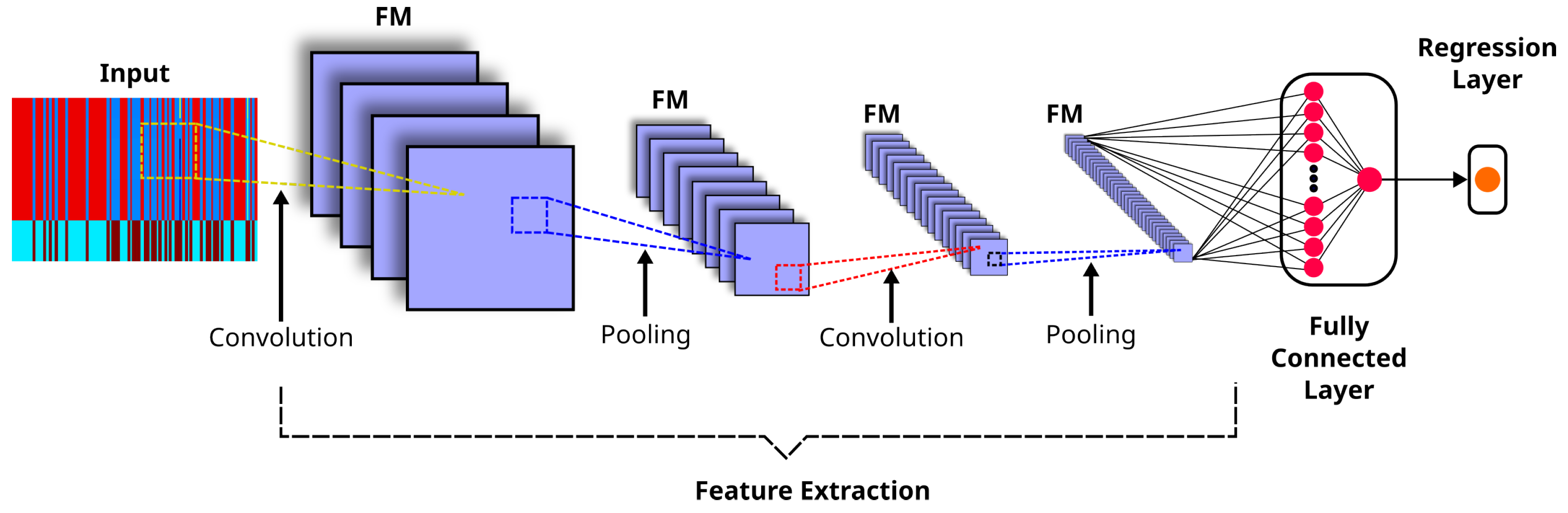
Appendix B. LSTM Models
LSTM models extend the memory capability of RNNs, enabling them to retain and learn long-term dependencies in sequential data. Specifically, they can preserve information over extended periods and perform fundamental memory operations, such as reading, writing, and deleting. This is possible because there are three gated cells corresponding to the fundamental memory operations: the input, output, and forget gates. The input gate controls whether new information is added to the memory, the output gate determines whether existing information contributes to the output, and the forget gate decides whether specific information is retained or discarded. The main characteristics of these three gates are described as follows [65]:
- Forget gate. It consists of a sigmoid function () that determines, based on and the current input (), which information should be removed from the memory. Equation (A1) shows the output of this gate:where and are the weight matrices of the forget gate, is a bias term and ranges from zero (discarding the learned information) to one (fully retaining it).
- Input gate. It is composed of a sigmoid activation layer () that selects values to update () and a tanh layer that generates candidate values () for the memory:where and are the weight matrices for the input gate, and and are the weight matrices for the candidate cell state.Thus, the memory is updated by multiplying the previous state () by the forget gate and adding the new candidate term () as shown in Equation (A4):
Appendix C. , Std MAE, and Metrics
On the one hand, measures the average magnitude of errors between predicted fHR values and reference fHR values ():
where
and
where M represents the number of measures.
On the other hand, measures the average squared difference between predicted fHR values () and reference fHR values (), providing greater emphasis on larger prediction errors through the squaring operation:
References
- Organización de las Naciones Unidas. Objetivos de Desarrolllo Sostenible; Technical Report; Organización de las Naciones Unidas: New York, NY, USA, 2015; Available online: https://www.un.org/sustainabledevelopment/es/ (accessed on 5 October 2024).
- Vican, I.; Kreković, G.; Jambrošić, K. Improved fetal heartbeat detection using pitch shifting and psychoacoustics. Biomed. Signal Process. Control 2024, 90, 105850. [Google Scholar] [CrossRef] [Scilit]
- Cesarelli, M.; Ruffo, M.; Romano, M.; Bifulco, P. Simulation of foetal phonocardiographic recordings for testing of FHR extraction algorithms. Comput. Methods Programs Biomed. 2012, 107, 513–523. [Google Scholar] [CrossRef] [Scilit]
- Jatia, N.; Veer, K. Techniques Used in Phonocardiography: A Review. In Lecture Notes in Mechanical Engineering; Springer: Singapore, 2022; pp. 79–90. [Google Scholar] [CrossRef] [Scilit]
- Ahmed, M.R.; Newby, S.; Potluri, P.; Mirihanage, W.; Fernando, A. Emerging Paradigms in Fetal Heart Rate Monitoring: Evaluating the Efficacy and Application of Innovative Textile-Based Wearables. Sensors 2024, 24, 66. [Google Scholar] [CrossRef] [Scilit]
- Tamber, K.K.; Hayes, D.J.; Carey, S.J.; Wijekoon, J.H.; Heazell, A.E. A systematic scoping review to identify the design and assess the performance of devices for antenatal continuous fetal monitoring. PLoS ONE 2020, 15, e0242983. [Google Scholar] [CrossRef] [Scilit]
- Altaf, A.; Mahdin, H.; Alive, A.M.; Ninggal, M.I.H.; Altaf, A.; Javid, I. Systematic Review for Phonocardiography Classification Based on Machine Learning. Int. J. Adv. Comput. Sci. Appl. 2023, 14, 806–817. [Google Scholar] [CrossRef] [Scilit]
- Burns, J.; Ganigara, M.; Dhar, A. Application of intelligent phonocardiography in the detection of congenital heart disease in pediatric patients: A narrative review. Prog. Pediatr. Cardiol. 2022, 64, 101455. [Google Scholar] [CrossRef] [Scilit]
- Sameni, R.; Samieinasab, M. Shiraz University Fetal Heart Sounds Database (Version 1.0.1). 2021. Available online: https://physionet.org/content/sufhsdb/1.0.1/ (accessed on 27 September 2024).
- Bhaskaran, A.; Sidhesh Kumar, J.; George, S.; Arora, M. Heart rate estimation and validation algorithm for fetal phonocardiography. Physiol. Meas. 2022, 43, 075008. [Google Scholar] [CrossRef] [Scilit]
- Bhaskaran, A.; Arora, M. Indian Institute of Science Fetal Heart Sound Database (IIScFHSDB) (Version 1.0). 2022. Available online: https://physionet.org/content/fetalheartsounddata/1.0/ (accessed on 27 September 2024).
- Barnova, K.; Kahankova, R.; Jaros, R.; Litschmannova, M.; Martinek, R. A comparative study of single-channel signal processing methods in fetal phonocardiography. PLoS ONE 2022, 17, e0269884. [Google Scholar] [CrossRef] [Scilit]
- Zhang, P.; Ye, S.; Huang, Z.; Jiaerken, D.; Zhao, S.; Zhang, L.; Wu, J. A noninvasive continuous fetal heart rate monitoring system for mobile healthcare based on fetal phonocardiography. In Internet of Things; Springer: Cham, Switzerland, 2019; pp. 191–204. [Google Scholar] [CrossRef] [Scilit]
- Chen, Y.; Wilkins, M.D.; Barahona, J.; Rosenbaum, A.J.; Daniele, M.; Lobaton, E. Toward Automated Analysis of Fetal Phonocardiograms: Comparing Heartbeat Detection from Fetal Doppler and Digital Stethoscope Signals. In Proceedings of the 2021 43rd Annual International Conference of the IEEE Engineering in Medicine & Biology Society (EMBC), Mexico City, Mexico, 1–5 November 2021; pp. 975–979. [Google Scholar] [CrossRef] [Scilit]
- Haque, E.; Gupta, T.; Singh, V.; Nene, K.; Masurkar, A. Detection and Classification of Fetal Heart Rate (FHR). Lect. Notes Electr. Eng. 2022, 836, 437–447. [Google Scholar] [CrossRef] [Scilit]
- Abburi, R.; Hatai, I.; Jaros, R.; Martinek, R.; Babu, T.A.; Babu, S.A.; Samanta, S. Adopting artificial intelligence algorithms for remote fetal heart rate monitoring and classification using wearable fetal phonocardiography. Appl. Soft Comput. 2024, 165, 112049. [Google Scholar] [CrossRef] [Scilit]
- Sbrollini, A.; Strazza, A.; Caragiuli, M.; Mozzoni, C.; Tomassini, S.; Agostinelli, A.; Morettini, M.; Fioretti, S.; Di Nardo, F.; Burattini, L. Fetal phonocardiogram denoising by wavelet transformation: Robustness to noise. In Proceedings of the Computing in Cardiology, Rennes, France, 24–27 September 2017; Volume 44, pp. 1–4. [Google Scholar] [CrossRef] [Scilit]
- Suryani Faradisa, I.; Ananda, A.; Arief Sardjono, T.; Hery Purnomo, M. Denoising of Fetal Phonocardiogram Signal by Wavelet Transformation. In Proceedings of the 4th International Conference on Electrical Systems, Technology and Information, ICESTI 2019, Bali, Indonesia, 24–27 October 2020; Volume 188. [Google Scholar] [CrossRef] [Scilit]
- Minani, G.; Malarvili, M. Fetal and Maternal Heart Sounds Denoising Based on Multi-level Discrete Wavelet Transform. In Proceedings of the 2023 13th International Conference on Biomedical Engineering and Technology, Tokyo, Japan, 15–18 June 2023; pp. 129–137. [Google Scholar] [CrossRef] [Scilit]
- Wang, Z.; Wei, J.; Li, X.; Liu, Z.; Su, F. Adaptive SVR Denoising Algorithm for Fetal Monitoring System. In Proceedings of the 2018 10th International Conference on Wireless Communications and Signal Processing (WCSP), Hangzhou, China, 18–20 October 2018. [Google Scholar] [CrossRef] [Scilit]
- Vadali, V.A.B.K.; Pandey, S.; Adithya, P.C.; Sankar, R. Fetal Phonocardiogram Decomposition Framework. In Proceedings of the SoutheastCon 2018, St. Petersburg, FL, USA, 19–22 April 2018; Volume 2018. [Google Scholar] [CrossRef] [Scilit]
- Cheikh, F.; Benhassine, N.E.; Sbaa, S. Fetal phonocardiogram signals denoising using improved complete ensemble (EMD) with adaptive noise and optimal thresholding of wavelet coefficients. Biomed. Tech. 2022, 67, 237–247. [Google Scholar] [CrossRef] [Scilit]
- Jatia, N.; Veer, K. Performance comparison of denoising methods for fetal phonocardiography using fir filter and empirical mode decomposition (EMD). In Optimization Methods for Engineering Problems; Apple Academic Press: Waretown, NJ, USA, 2023; pp. 171–183. [Google Scholar]
- Pauline, S.H.; Dhanalakshmi, S.; Kumar, R.; Narayanamoorthi, R.; Lai, K.W. A Low-Cost Multistage Cascaded Adaptive Filter Configuration for Noise Reduction in Phonocardiogram Signal. J. Healthc. Eng. 2022, 2022, 3039624. [Google Scholar] [CrossRef] [Scilit]
- Taralunga, D.D.; Tautan, A.M.; Ungureanu, G.M. An Efficient Method for Fetal Heart Sounds Detection Based on Hilbert Transform. In Proceedings of the 2018 International Conference and Exposition on Electrical and Power Engineering (EPE), Iasi, Romania, 18–19 October 2018; pp. 916–919. [Google Scholar] [CrossRef] [Scilit]
- Taralunga, D.D.; Mihaela Neagu Ungureanu, G. An ensemble empirical mode decomposition based method for fetal phonocardiogram enhancement. In World Congress on Medical Physics and Biomedical Engineering 2018. IFMBE Proceedings; Springer: Singapore, 2018; Volume 68, pp. 387–391. [Google Scholar] [CrossRef] [Scilit]
- Tomassini, S.; Strazza, A.; Sbrollini, A.; Marcantoni, I.; Morettini, M.; Fioretti, S.; Burattini, L. Wavelet filtering of fetal phonocardiography: A comparative analysis. Math. Biosci. Eng. 2019, 16, 6034–6046. [Google Scholar] [CrossRef] [Scilit]
- Strazza, A.; Sbrollini, A.; Olivastrelli, M.; Piersanti, A.; Tomassini, S.; Marcantoni, I.; Morettini, M.; Fioretti, S.; Burattini, L. PCG-Decompositor: A New Method for Fetal Phonocardiogram Filtering Based on Wavelet Transform Multi-level Decomposition. In XV Mediterranean Conference on Medical and Biological Engineering and Computing; Springer International Publishing: Cham, Switzerland, 2020; Volume 76, pp. 47–53. [Google Scholar] [CrossRef] [Scilit]
- Martinek, R.; Barnova, K.; Jaros, R.; Kahankova, R.; Kupka, T.; Jezewski, M.; Czabanski, R.; Matonia, A.; Jezewski, J.; Horoba, K. Passive Fetal Monitoring by Advanced Signal Processing Methods in Fetal Phonocardiography. IEEE Access 2020, 8, 221942–221962. [Google Scholar] [CrossRef] [Scilit]
- Zhdanov, D.; Zemlyakov, I.Y.; Kosteley, Y.V.; Bureev, A.S. Choice of Wavelet Filtering Parameters for Processing Fetal Phonocardiograms with High Noise Level. Biomed. Eng. 2021, 55, 194–198. [Google Scholar] [CrossRef] [Scilit]
- Kong, L.; Barnova, K.; Jaros, R.; Mirjalili, S.; Snasel, V.; Pan, J.S.; Martinek, R. Analysis on fetal phonocardiography segmentation problem by hybridized classifier. Eng. Appl. Artif. Intell. 2024, 135, 108621. [Google Scholar] [CrossRef] [Scilit]
- Bhaskaran, A.; Arora, M. Evaluation of cyclic repetition frequency based algorithm for fetal heart rate extraction from fetal phonocardiography. Biomed. Signal Process. Control 2024, 88, 105010. [Google Scholar] [CrossRef] [Scilit]
- Zhdanov, D.S.; Bureev, A.S.; Kutsov, M.S.; Kiseleva, E.Y.; Kistenev, Y.V. Algorithm for extraction of fetal heart tones during fetal phonocardiography. Biol. Med. 2015, 7, 1–5. [Google Scholar]
- Tang, H.; Li, T.; Qiu, T.; Park, Y. Fetal Heart Rate Monitoring from Phonocardiograph Signal Using Repetition Frequency of Heart Sounds. J. Electr. Comput. Eng. 2016, 2016, 2404267. [Google Scholar] [CrossRef] [Scilit]
- Shabry, N.A.N.B.M.; Singh, O.; Sardana, P.; Hisham, R.B.; Malarvili, M. Home based fetal heart rate monitor. Int. J. Appl. Eng. Res. 2017, 12, 813–817. [Google Scholar]
- Koutsiana, E.; Hadjileontiadis, L.; Khandoker, A.H.; Chouvarda, I. A Comparative Phonocardiography Study: Two Wavelet Based Methods for Fetal Heart Sound Detection. In Proceedings of the 2018 Computing in Cardiology Conference (CinC), Maastricht, The Netherlands, 23–26 September 2018; Volume 2018. [Google Scholar] [CrossRef] [Scilit]
- Atteeq, M.; Khan, M.F.; Qureshi, A.N. Fetus heart beat extraction from mother’s PCG using blind source separation. In Proceedings of the 2019 11th International Conference on Bioinformatics and Biomedical Technology, Stockholm, Sweden, 29–31 May 2019; pp. 100–104. [Google Scholar] [CrossRef] [Scilit]
- Setiawan, A.W.; Sujatmiko, W. Comparison of Fetal Heart Rate Detection Using Envelope Extraction and Shannon Energy. In Proceedings of the 2019 International Seminar on Application for Technology of Information and Communication (iSemantic), Semarang, Indonesia, 21–22 September 2019; pp. 446–449. [Google Scholar] [CrossRef] [Scilit]
- Dia, N.; Fontecave-Jallon, J.; Gumery, P.Y.; Rivet, B. Fetal heart rate estimation from a single phonocardiogram signal using non-negative matrix factorization. In Proceedings of the 2019 41st Annual International Conference of the IEEE Engineering in Medicine and Biology Society (EMBC), Berlin, Germany, 23–27 July 2019; pp. 5983–5986. [Google Scholar] [CrossRef] [Scilit]
- Rojas, M.R.; Rivet, B.; Kavouni, N.M.; Fontecave-Jallon, J. Phonocardiography for robust fetal heart rate estimation in real clinical conditions. Biomed. Signal Process. Control 2025, 107, 107807. [Google Scholar] [CrossRef] [Scilit]
- Wang, H.; Liang, X. Extraction Method of Fetal Phonocardiogram Based on Lifting wavelet analysis. J. Phys. Conf. Ser. 2020, 1544, 012103. [Google Scholar] [CrossRef] [Scilit]
- Vican, I.; Kreković, G.; Jambrošić, K. Can empirical mode decomposition improve heartbeat detection in fetal phonocardiography signals? Comput. Methods Programs Biomed. 2021, 203, 106038. [Google Scholar] [CrossRef] [Scilit]
- Sharma, Y.; Ray, S.; Yadav, O.P. Transformative Advancements in Fetal Cardiac Health on BiLSTM Networks for FPCG Classification. Radioelectron. Commun. Syst. 2024, 67, 265–275. [Google Scholar] [CrossRef] [Scilit]
- Spadaccini, A.; Beritelli, F. Performance evaluation of heart sounds biometric systems on an open dataset. In Proceedings of the 2013 18th International Conference on Digital Signal Processing (DSP); IEEE: Piscataway, NJ, USA, 2013; pp. 1–5. [Google Scholar]
- Oliveira, J.; Renna, F.; Costa, P.; Nogueira, M.; Oliveira, A.C.; Elola, A.; Ferreira, C.; Jorge, A.; Rad, A.B.; Reyna, M.; et al. The CirCor DigiScope Dataset: From Murmur Detection to Murmur Classification. IEEE J. Biomed. Health Inform. 2022, 26, 2524–2535. [Google Scholar] [CrossRef] [Scilit]
- Bentley, P.; Nordehn, G.; Coimbra, M.; Mannor, S. The PASCAL Classifying Heart Sounds Challenge 2011 (CHSC2011) Results. Available online: http://www.peterjbentley.com/heartchallenge/index.html (accessed on 5 October 2024).
- Goldberger, A.L.; Amaral, L.A.; Glass, L.; Hausdorff, J.M.; Ivanov, P.C.; Mark, R.G.; Mietus, J.E.; Moody, G.B.; Peng, C.K.; Stanley, H.E. PhysioBank, PhysioToolkit, and PhysioNet: Components of a new research resource for complex physiologic signals. Circulation 2000, 101, e215–e220. [Google Scholar]
- Cesarelli, M.; Ruffo, M.; Romano, M.; Bifulco, P.; Fratini, A. Fetal PCGs. 2015. Available online: https://archive.physionet.org/pn3/fpcgdb/ (accessed on 27 September 2024).
- Martinek, R.; Jaros, R.; Kahankova, R.; Barnova, K. Synthetic Fetal PCG Signals; IEEE Dataport: Piscataway, NJ, USA, 2020. [Google Scholar] [CrossRef]
- Amrutha, B.; Sinha, R.; Kumar, S.; Arora, M. Foetal Acoustic Simulator. In Proceedings of the 2019 11th International Conference on Communication Systems & Networks (COMSNETS), Bangalore, India, 7–11 January 2019; pp. 882–885. [Google Scholar]
- Martens, J.B. The Hermite transform-theory. IEEE Trans. Acoust. Speech Signal Process. 1990, 38, 1595–1606. [Google Scholar] [CrossRef]
- Martens, J.B. The Hermite transform-applications. IEEE Trans. Acoust. Speech Signal Process. 1990, 38, 1607–1618. [Google Scholar] [CrossRef] [Scilit]
- Gomez-Coronel, S.L.; Escalante-Ramirez, B.; Acevedo-Mosqueda, M.A.; Mosqueda, M.E.A. Steganography in audio files by Hermite Transform. Appl. Math. Inf. Sci. 2014, 8, 959. [Google Scholar] [CrossRef] [Scilit]
- Moya-Albor, E.; Brieva, J.; Ponce, H.; Rivas-Scott, O.; Gómez-Peña, C. Heart Rate Estimation using Hermite Transform Video Magnification and Deep Learning. In Proceedings of the 2018 40th Annual International Conference of the IEEE Engineering in Medicine and Biology Society (EMBC), Honolulu, HI, USA, 18–21 July 2018; pp. 2595–2598. [Google Scholar] [CrossRef] [Scilit]
- Barba-J, L.; Escalante-Ramírez, B.; Vallejo Venegas, E.; Arámbula Cosío, F. A 3D Hermite-based multiscale local active contour method with elliptical shape constraints for segmentation of cardiac MR and CT volumes. Med. Biol. Eng. Comput. 2018, 56, 833–851. [Google Scholar] [CrossRef] [Scilit]
- Siuly, S.; Alcin, O.F.; Bajaj, V.; Sengur, A.; Zhang, Y. Exploring Hermite transformation in brain signal analysis for the detection of epileptic seizure. IET Sci. Meas. Technol. 2019, 13, 35–41. [Google Scholar] [CrossRef] [Scilit]
- Bracewell, R.N. The Fourier Transform and Its Applications, 3rd ed.; McGraw-Hill: New York, NY, USA, 2000. [Google Scholar]
- Oppenheim, A.V.; Schafer, R.W. Discrete-Time Signal Processing, 3rd ed.; Prentice Hall: Englewood Cliffs, NJ, USA, 2010. [Google Scholar]
- Papoulis, A. The Fourier Integral and Its Applications; McGraw-Hill: New York, NY, USA, 1962. [Google Scholar]
- Boashash, B. Estimating and interpreting the instantaneous frequency of a signal. I. Fundamentals. Proc. IEEE 1992, 80, 520–538. [Google Scholar] [CrossRef] [Scilit]
- Zheng, F.; Zhang, G.; Song, Z. Comparison of different implementations of MFCC. J. Comput. Sci. Technol. 2001, 16, 582–589. [Google Scholar] [CrossRef] [Scilit]
- Abdul, Z.K.; Al-Talabani, A.K. Mel frequency cepstral coefficient and its applications: A review. IEEE Access 2022, 10, 122136–122158. [Google Scholar] [CrossRef] [Scilit]
- He, K.; Zhang, X.; Ren, S.; Sun, J. Deep Residual Learning for Image Recognition. In Proceedings of the IEEE Conference on Computer Vision and Pattern Recognition (CVPR), Las Vegas, NV, USA, 27–30 June 2016; pp. 770–778. [Google Scholar]
- Tharwat, A. From Perceptrons to Convolutional Neural Networks: A Practical Tutorial on Spatial Deep Learning. Mathematics 2026, 14, 2822. [Google Scholar] [CrossRef] [Scilit]
- Siami-Namini, S.; Tavakoli, N.; Namin, A.S. The Performance of LSTM and BiLSTM in Forecasting Time Series. In Proceedings of the 2019 IEEE International Conference on Big Data (Big Data), Los Angeles, CA, USA, 9–12 December 2019; pp. 3285–3292. [Google Scholar] [CrossRef] [Scilit]
- Maddirala, A.K.; Shaik, R.A. Motion artifact removal from single channel electroencephalogram signals using singular spectrum analysis. Biomed. Signal Process. Control 2016, 30, 79–85. [Google Scholar] [CrossRef] [Scilit]
- Brajović, M.; Stanković, S.; Orović, I. Analysis of noisy coefficients in the discrete Hermite transform domain with application in signal denoising and sparse signal reconstruction. Signal Process. 2018, 150, 145–156. [Google Scholar] [CrossRef] [Scilit]
- Bhaskaran, A.; Arora, M. Automatic filter selection for Hilbert autocorrelation and cyclic repetition frequency based fPCG analysis. Biomed. Signal Process. Control 2024, 92, 106018. [Google Scholar] [CrossRef] [Scilit]
- Moraes, H.; Carvalho, R.; Colonna, J.; Nakamura, E. Fetal Heart Rate Estimation in Phonocardiograms Using Deep Learning and Digital Signal Processing. In Proceedings of the 31st Brazilian Symposium on Multimedia and the Web, Rio de Janeiro, Brazil, 10–14 November 2025; pp. 258–266. [Google Scholar] [CrossRef] [Scilit]
- Pstras, L.; Okupnik, T.; Ponikowska, B.; Paleczny, B. Facial video photoplethysmography for measuring average and quasi-instantaneous heart rate: A pilot validation study. Front. Physiol. 2025, 16, 1638809. [Google Scholar] [CrossRef] [Scilit]
- National Guideline Alliance (UK). Addendum to Intrapartum Care: Care for Healthy Women and Babies; NICE Clinical Guideline 190.1; National Institute for Health and Care Excellence (NICE): London, UK, 2017; Appendix J: Fetal heart rate classifications.
- Holdsworth, J.; Scapicchio, M. What Is Deep Learning? 2024. Available online: https://www.ibm.com/topics/deep-learning (accessed on 27 September 2024).
- Yosinski, J.; Clune, J.; Bengio, Y.; Lipson, H. How transferable are features in deep neural networks? In Proceedings of the Advances in Neural Information Processing Systems 27 (NIPS ’14); Ghahramani, Z., Welling, M., Cortes, C., Lawrence, N., Weinberger, K., Eds.; Curran Associates, Inc.: Red Hook, NY, USA, 2014; pp. 3320–3328. [Google Scholar]
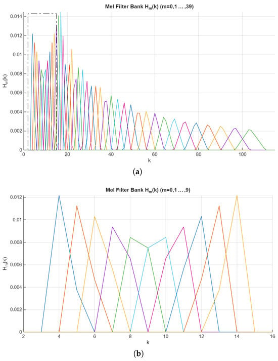
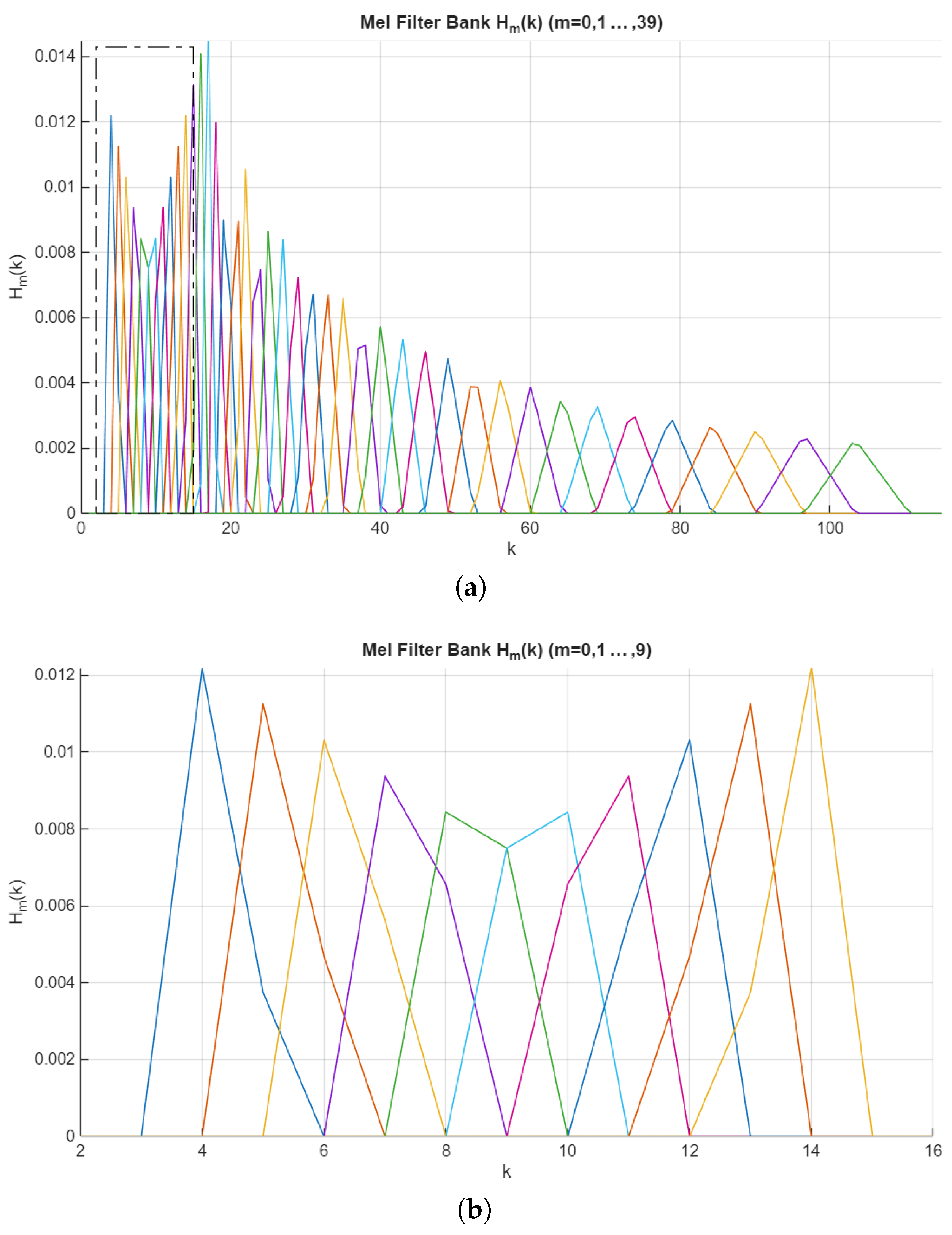
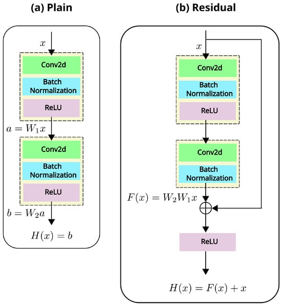
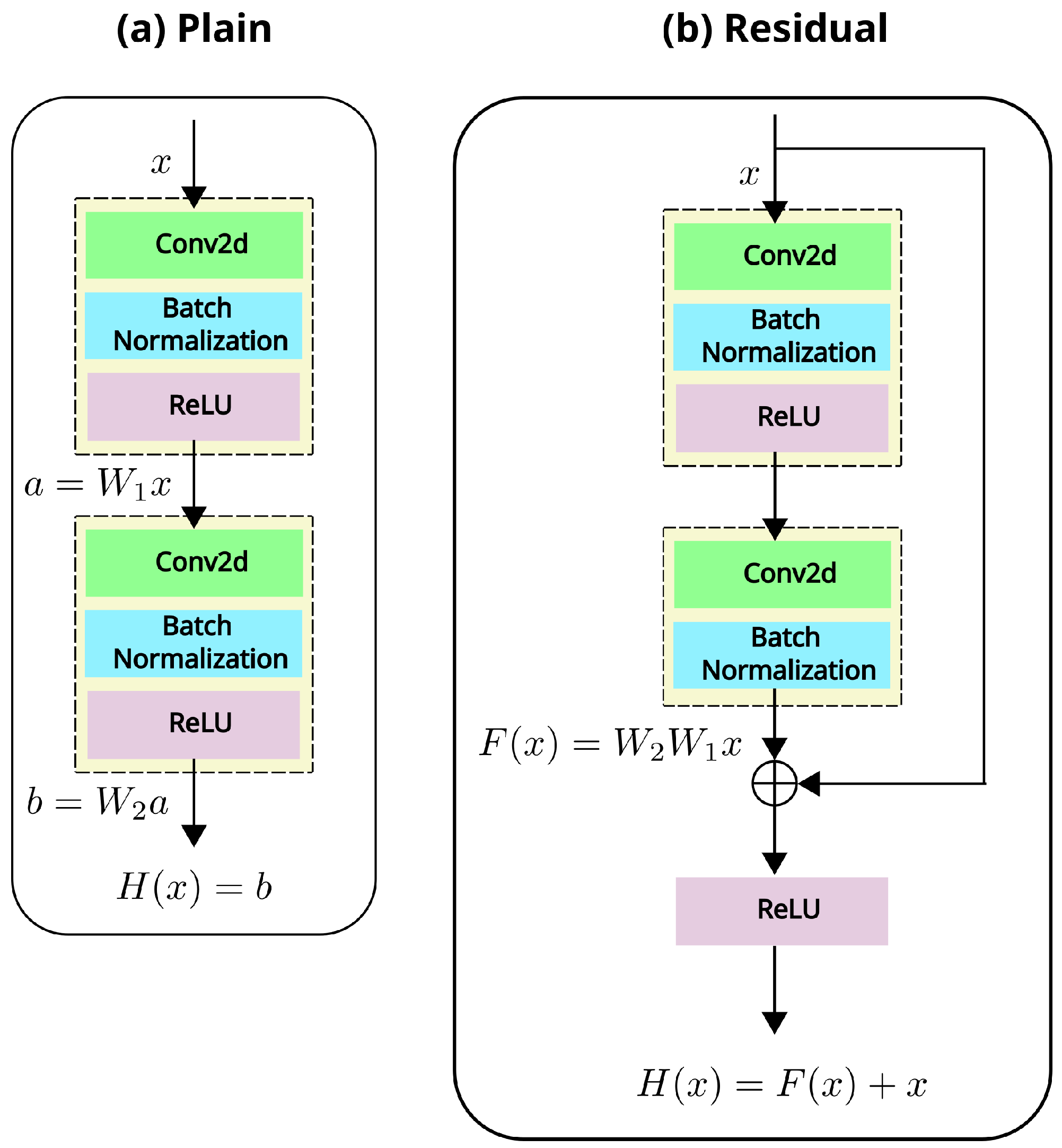
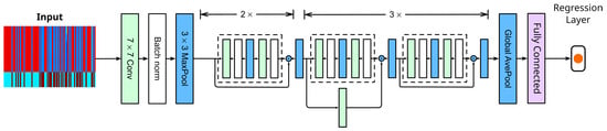
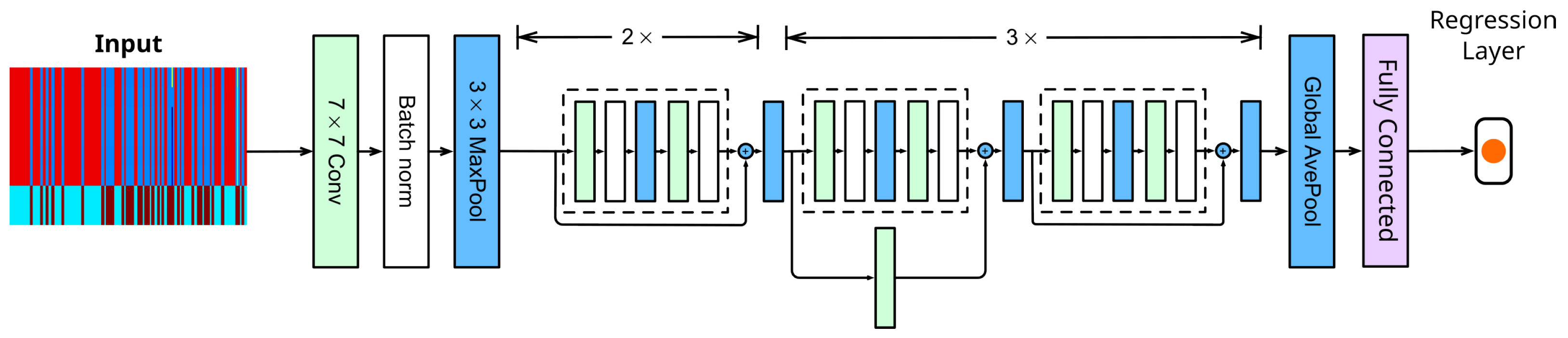
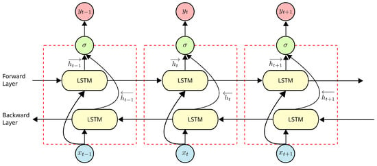
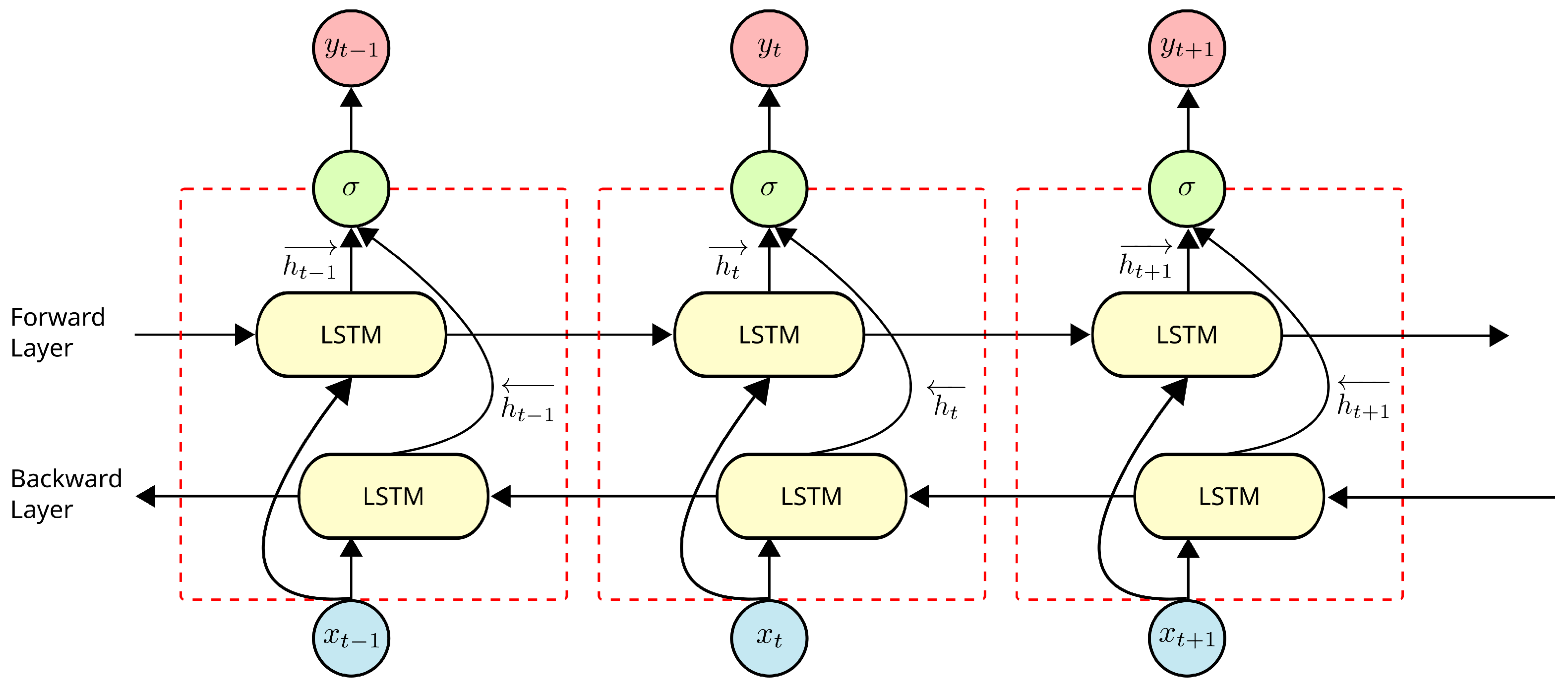
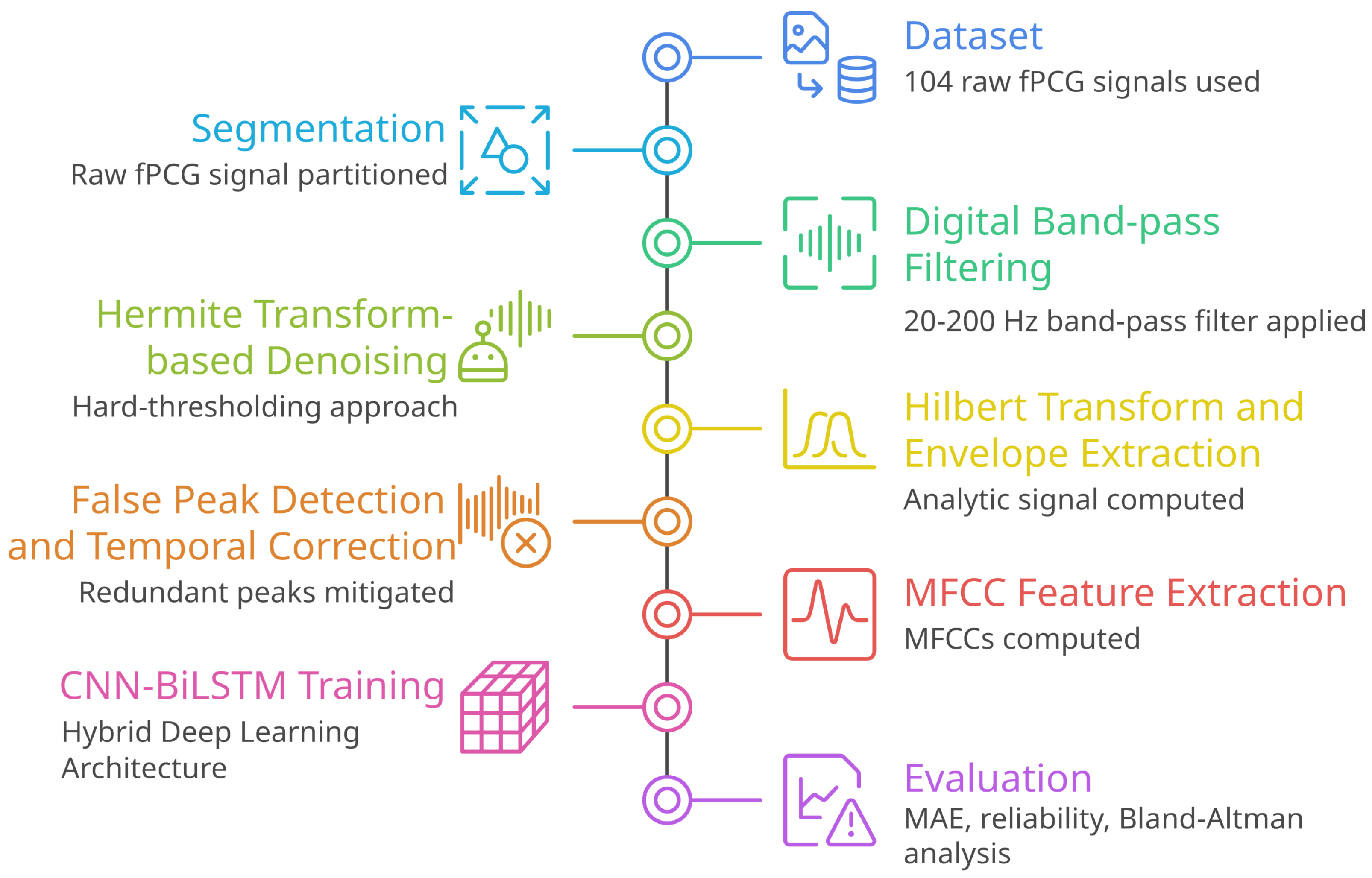
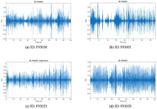
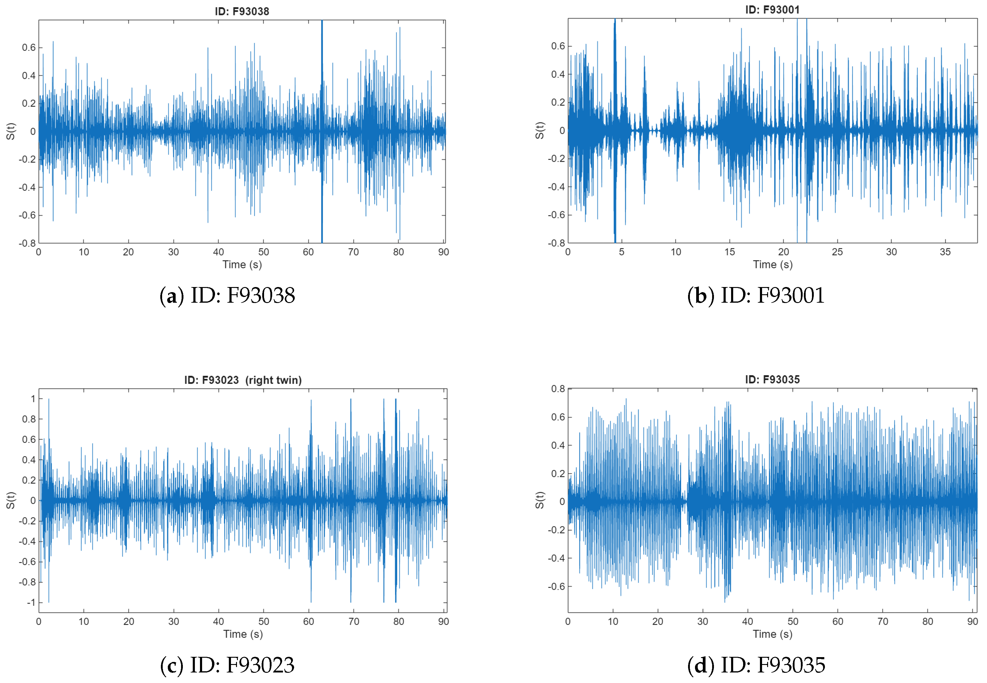
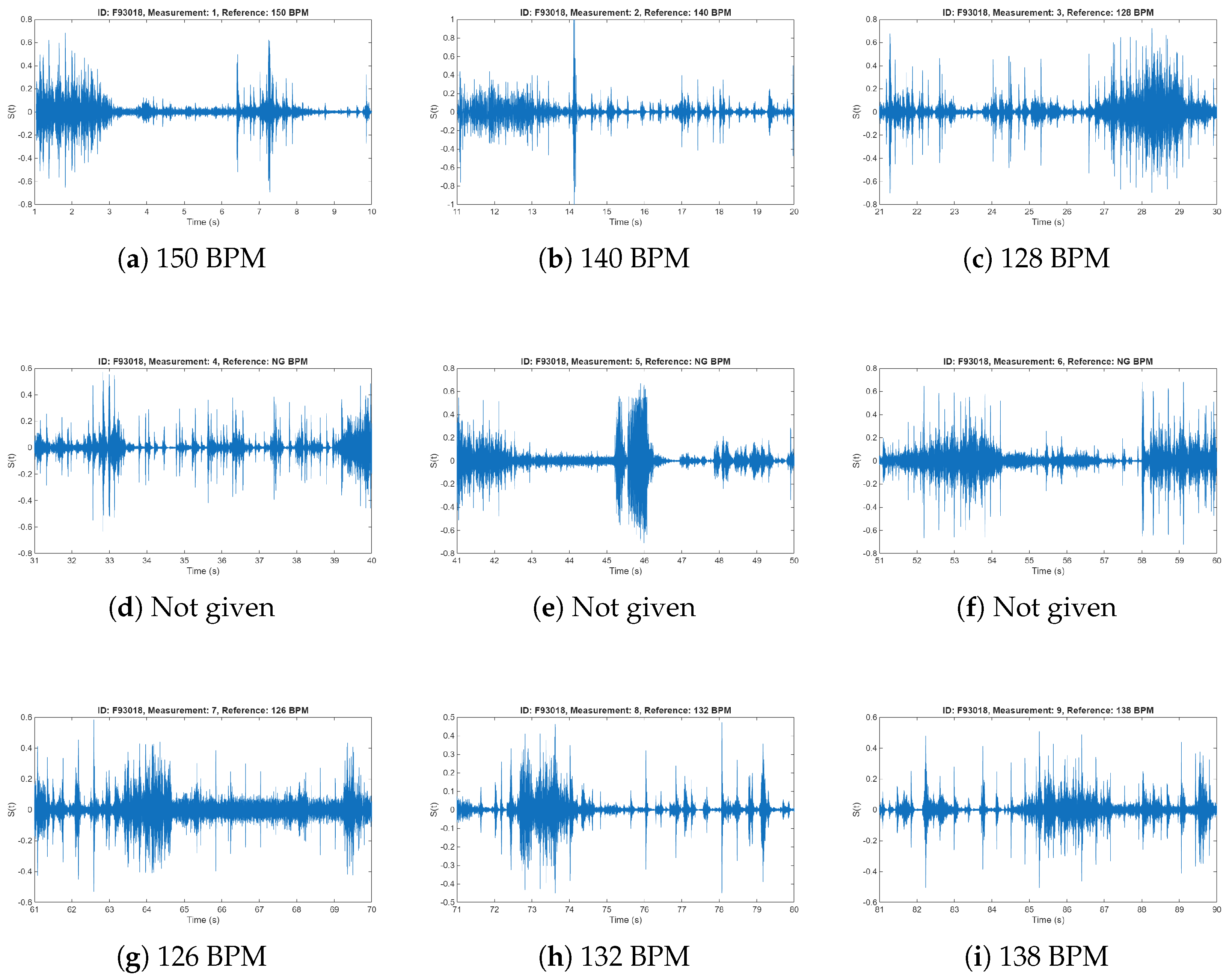
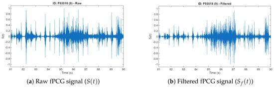
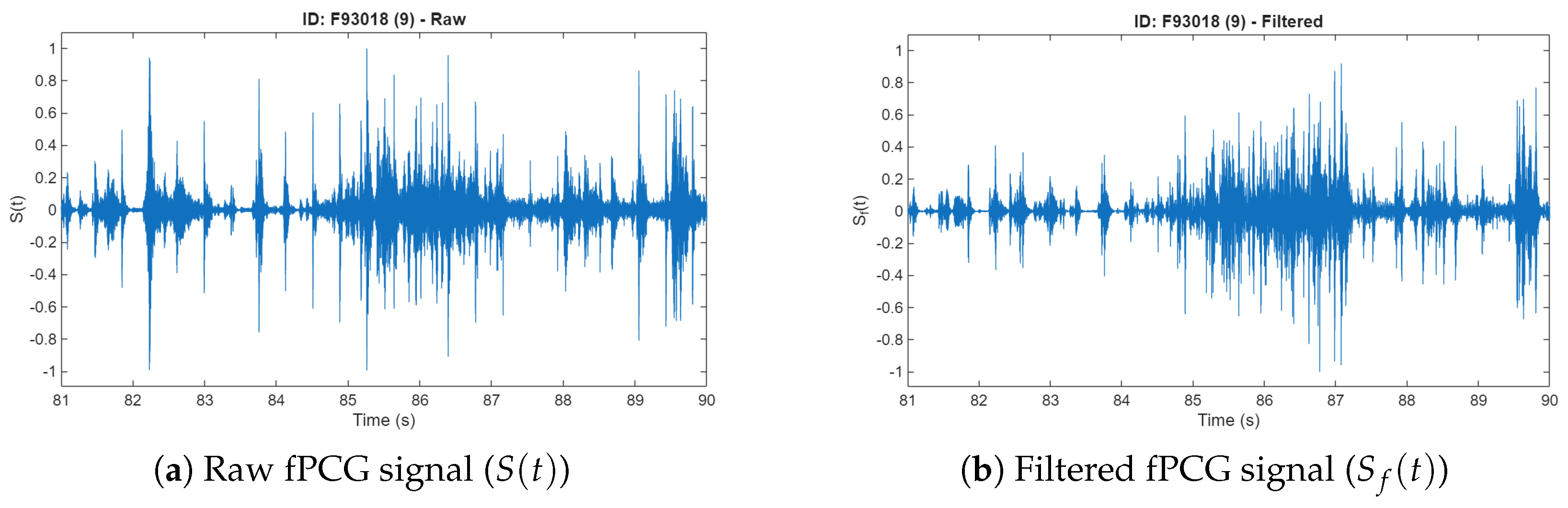
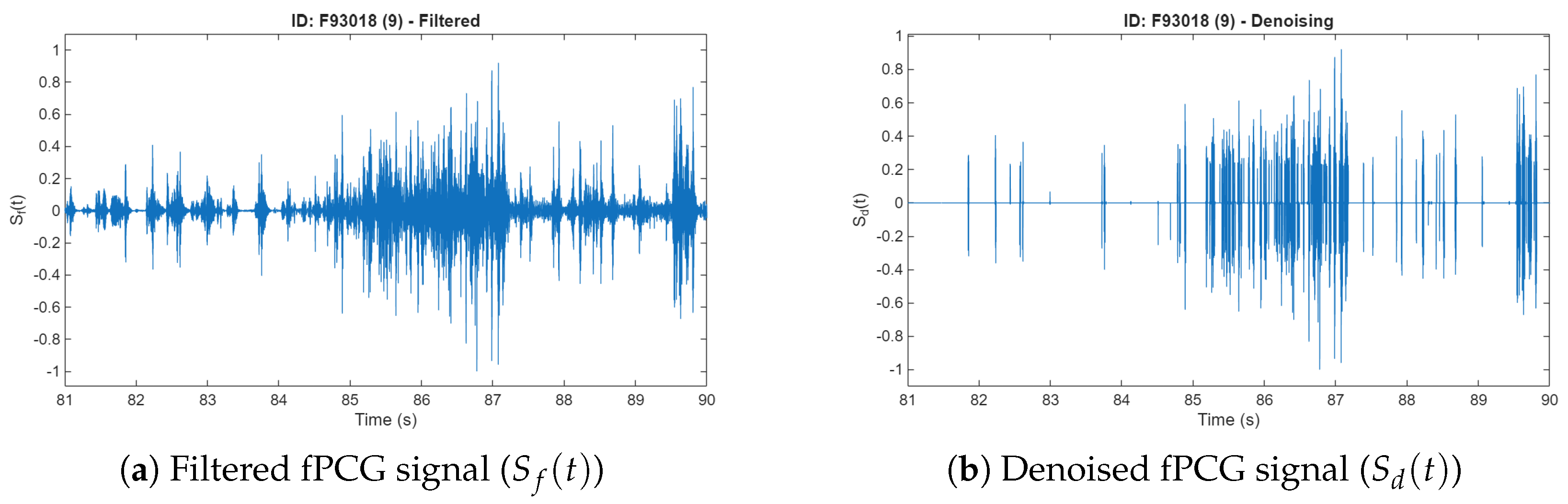
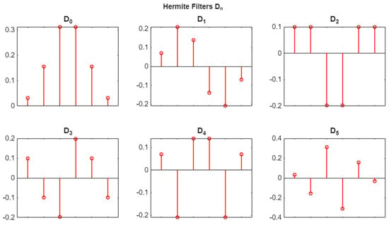
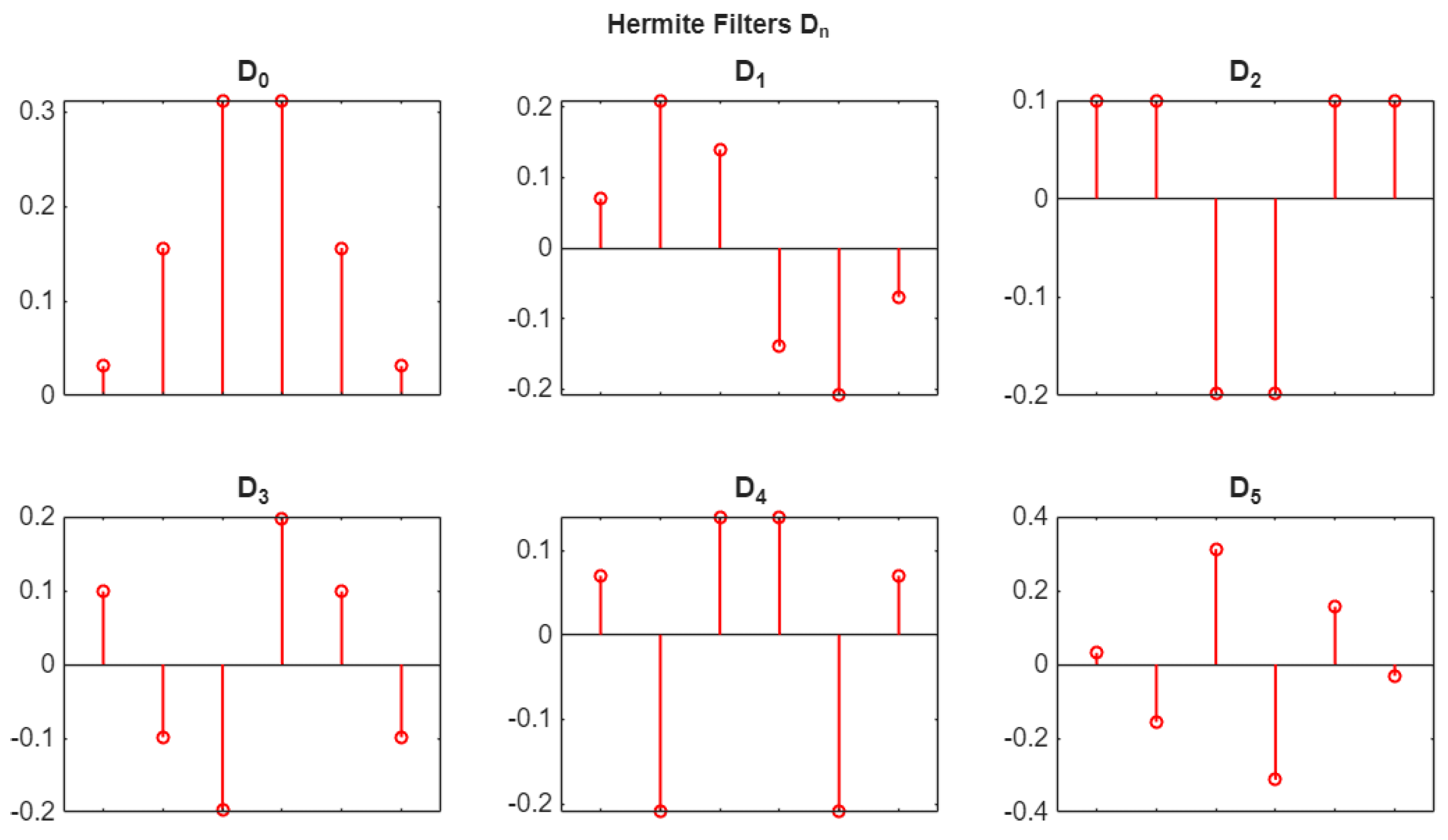
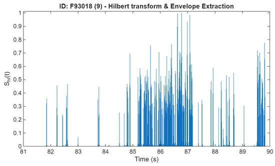
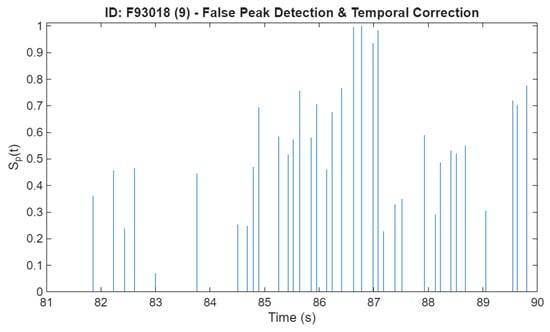
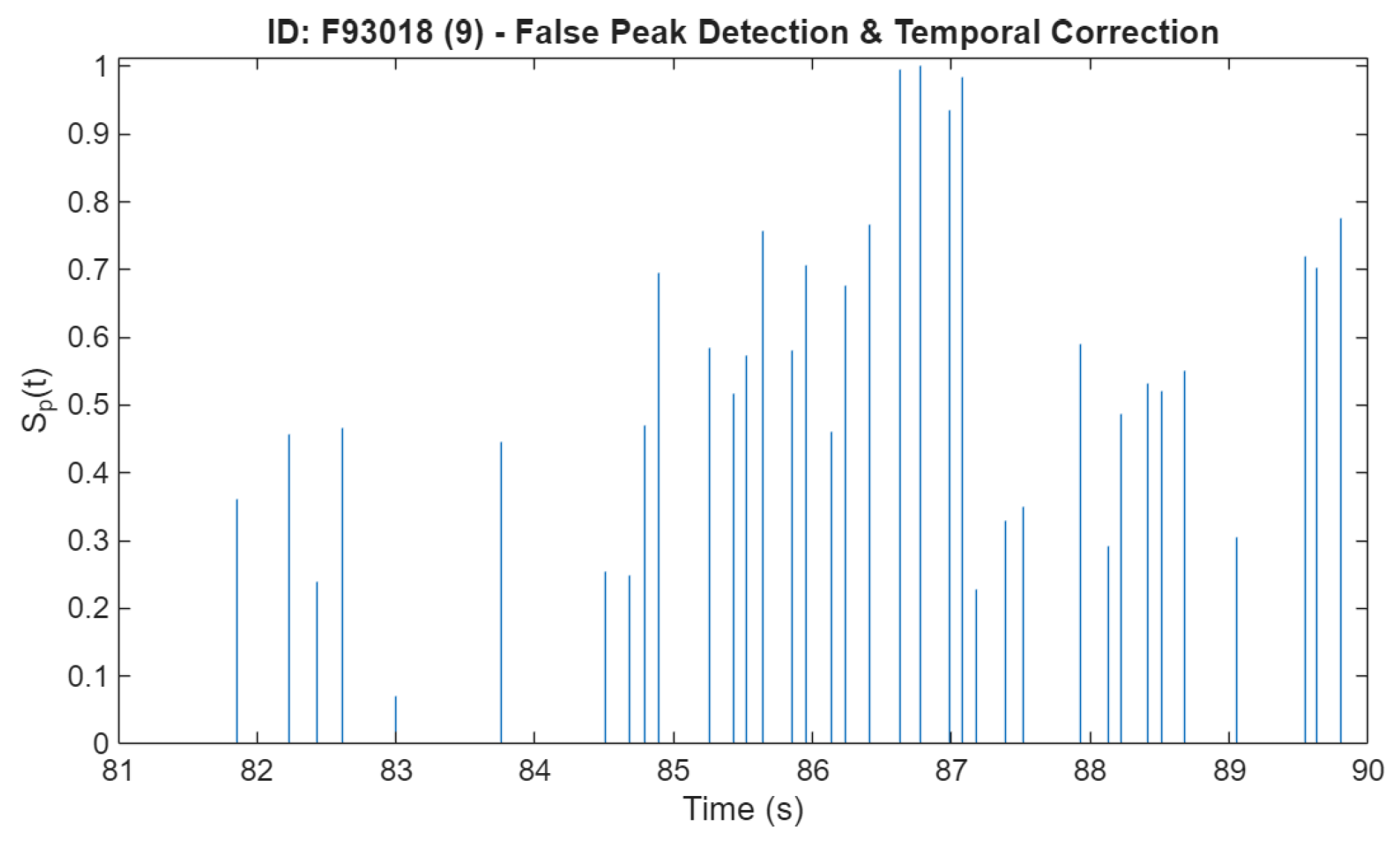
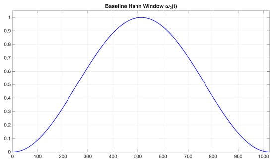
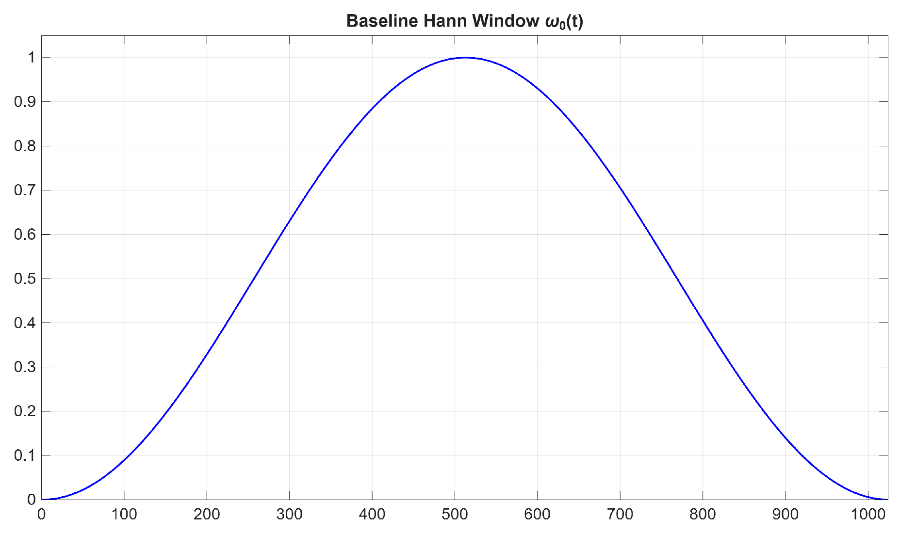
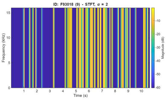
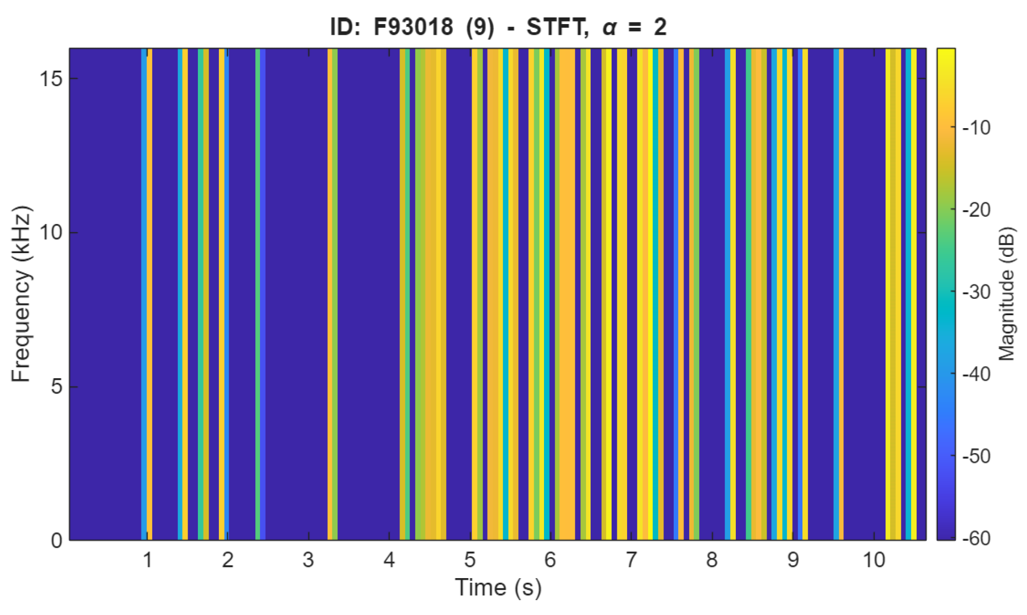
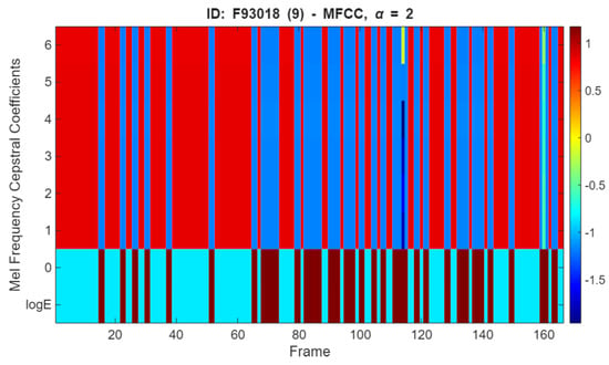
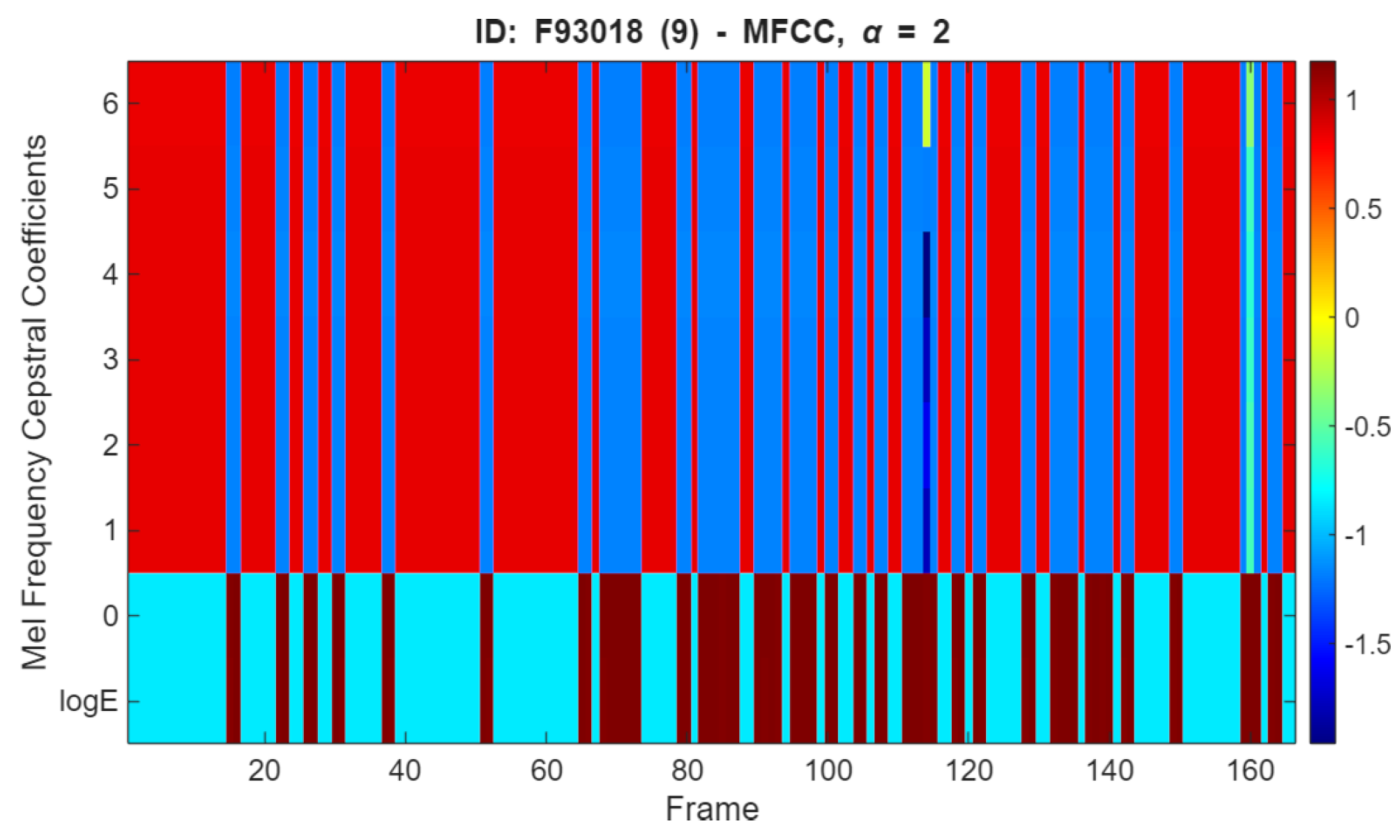
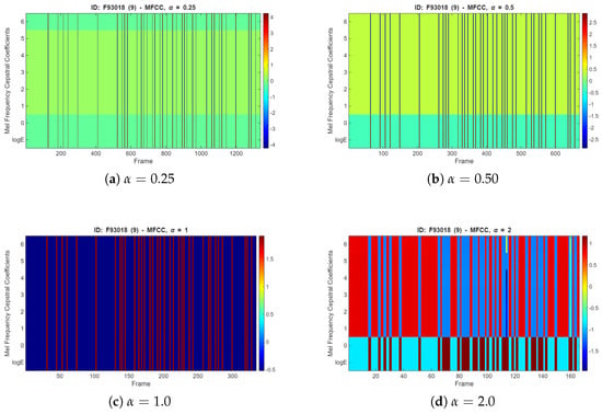
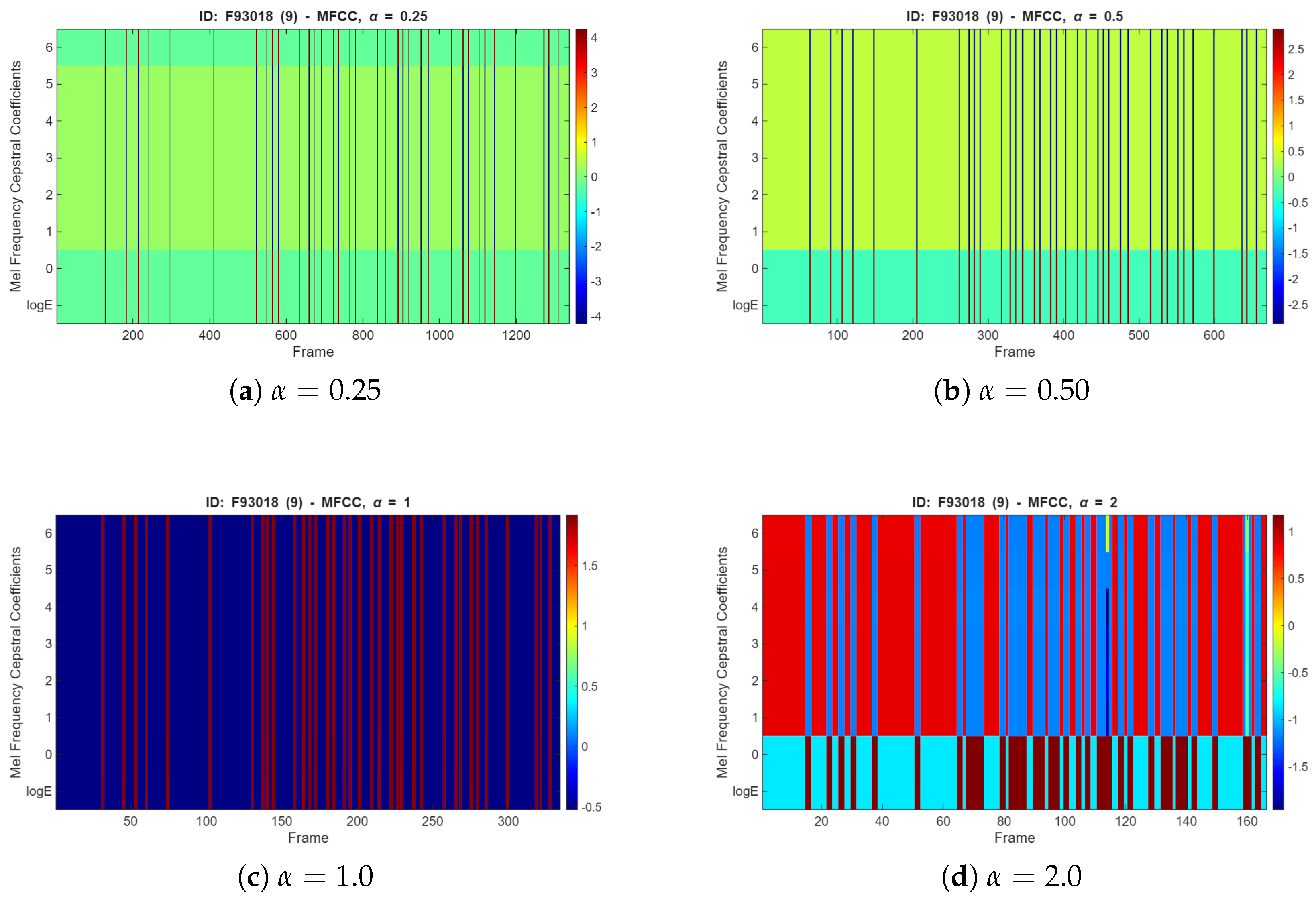
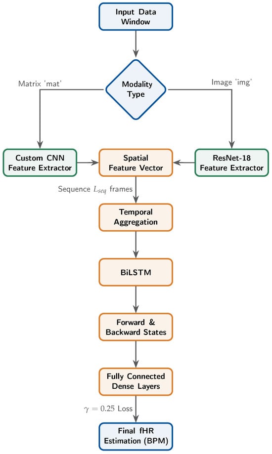
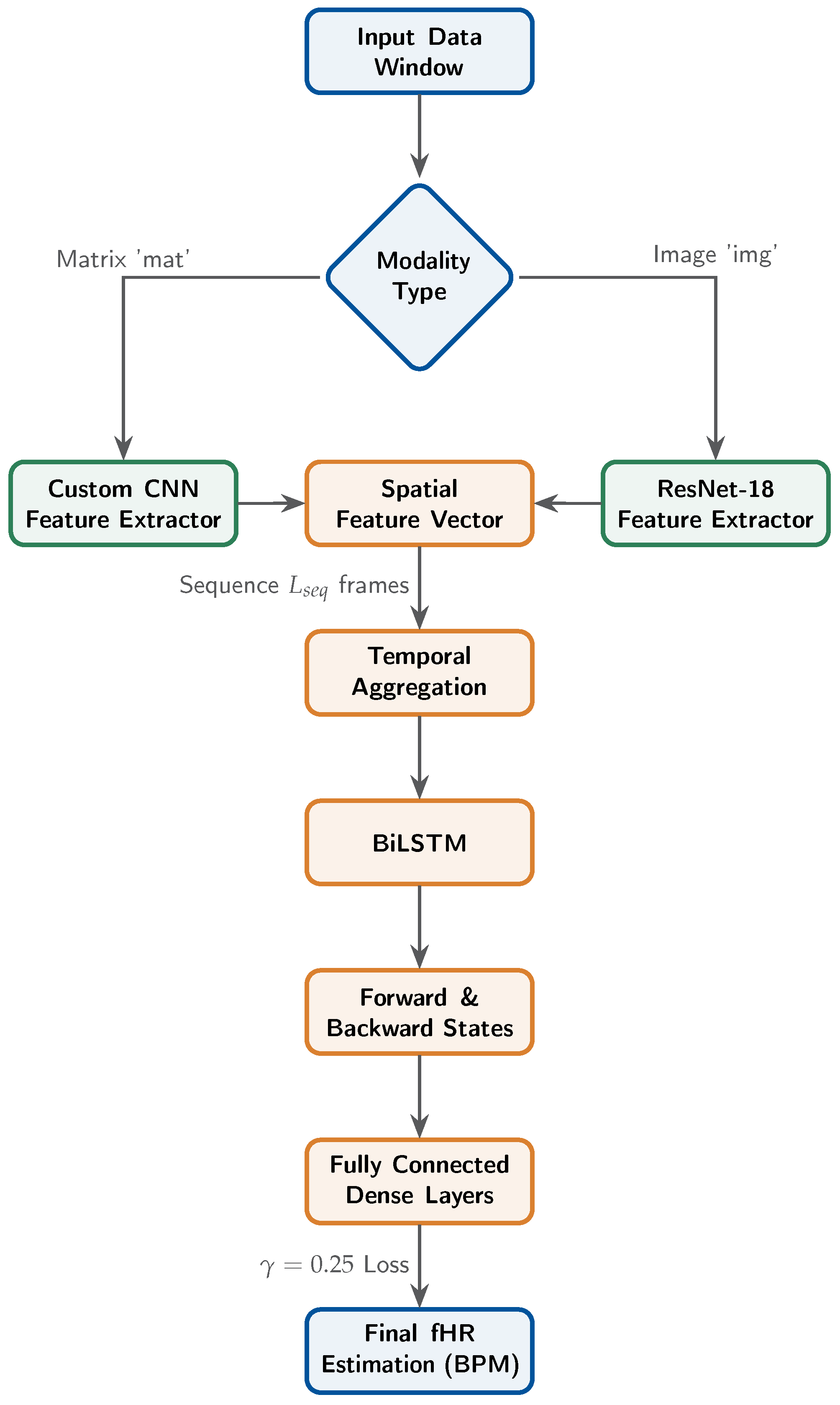
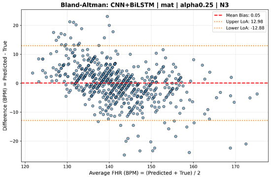
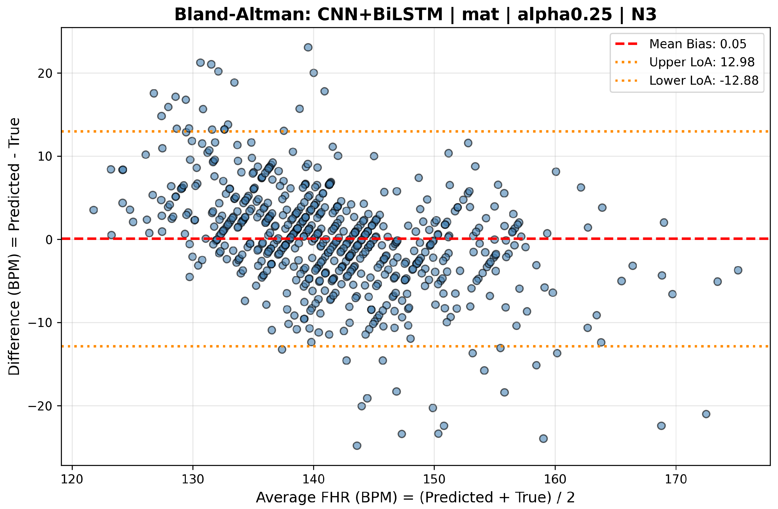
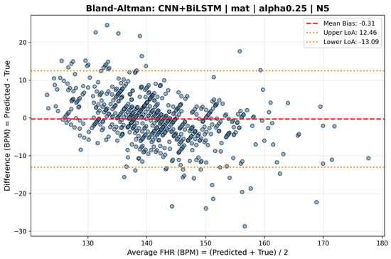
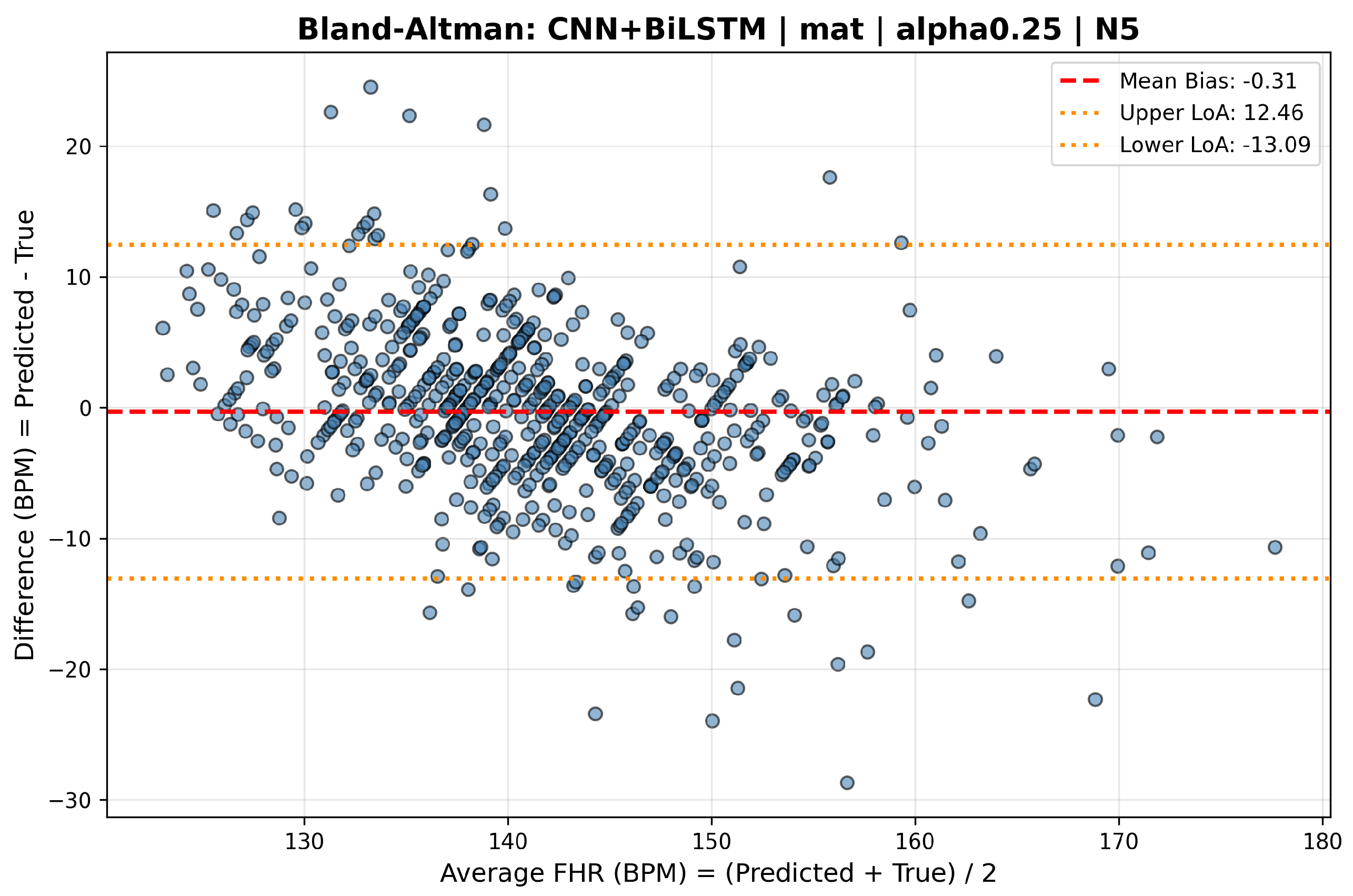
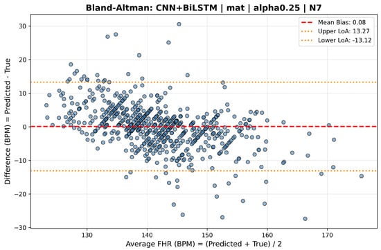
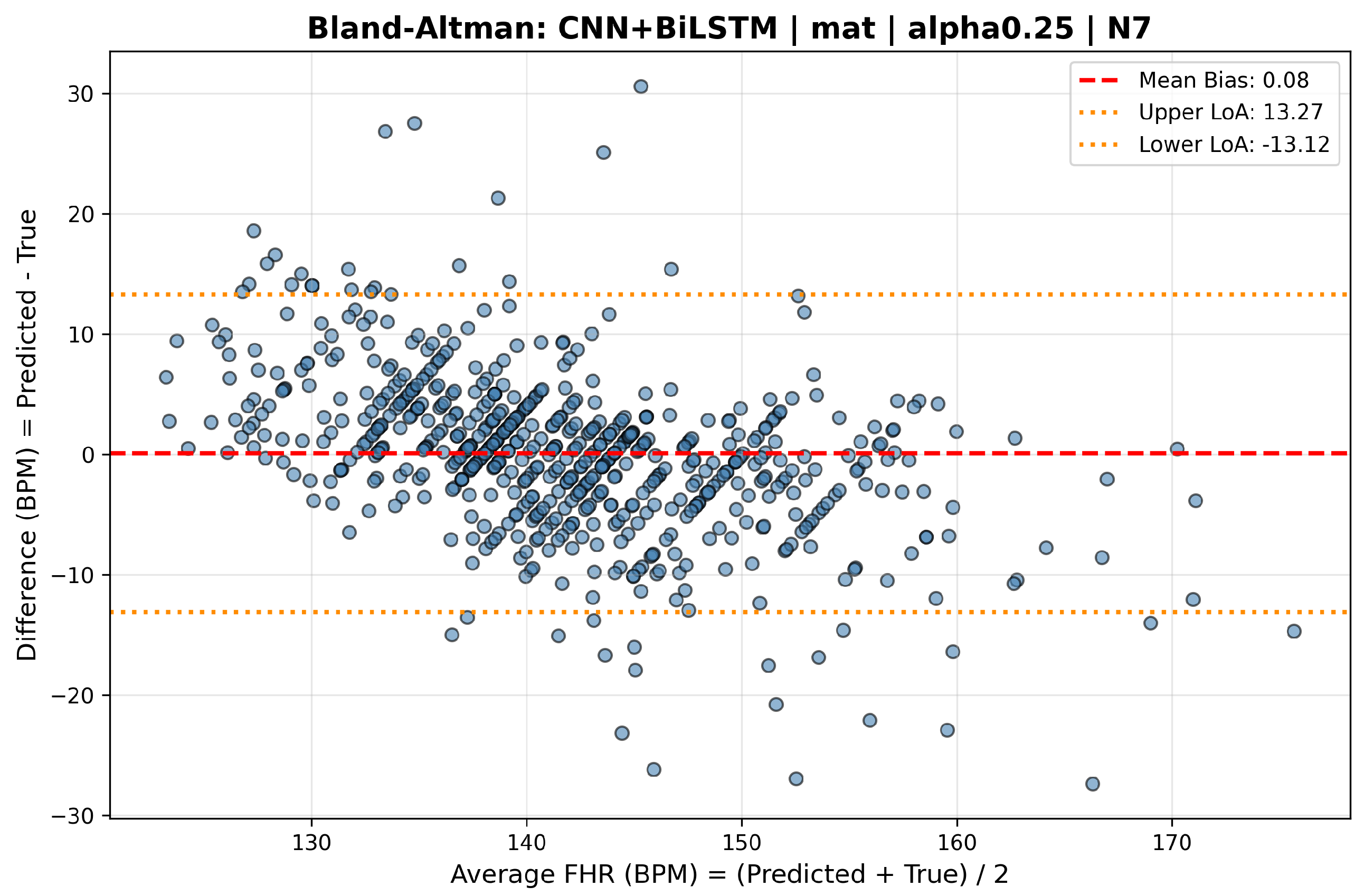

Disclaimer/Publisher’s Note: The statements, opinions and data contained in all publications are solely those of the individual author(s) and contributor(s) and not of MDPI and/or the editor(s). MDPI and/or the editor(s) disclaim responsibility for any injury to people or property resulting from any ideas, methods, instructions or products referred to in the content. |
© 2026 by the authors. Licensee MDPI, Basel, Switzerland. This article is an open access article distributed under the terms and conditions of the Creative Commons Attribution (CC BY) license.