Variable-Order Fuzzy Fractional PID Control in a Reduced Quadrotor Altitude Benchmark: Paired Monte Carlo Evaluation and Mechanism-Oriented Analysis

Abstract

This paper compares fixed-order (FO) and variable-order (VO) fuzzy fractional PID control in a reduced numerical benchmark for quadrotor altitude tracking. The study asks whether online order scheduling changes paired performance when the fuzzy gain structure, gain channels, fractional approximation, plant, reference, random realizations, and evaluation protocol are fixed. The benchmark comprises vertical double-integrator dynamics, a first-order actuator lag, and asymmetric clipping of an equivalent net-thrust command; it is not full-vehicle or hardware validation. Both controllers use the same two-input, five-output Sugeno structure. FO is optimized first, and VO then optimizes four scheduling parameters while retaining the FO gain channels. Evaluation uses a six-segment reference, a composite index, 100 pre-specified paired Monte Carlo seeds, paired effect estimates, two counterfactual order variants, and an existing stronger-disturbance test without retraining. At baseline, VO reduces mean J by 3.97%, ITAE by 7.06%, positive-upper-limit near-saturation exposure by 43.36%, and RMS input by 3.18% while increasing the total in-band ratio by 6.80%. Overshoot and robust settling time show no statistically supported improvement. The counterfactual results are more consistent with state-dependent variation than a fixed-order shift alone but do not form an additive causal decomposition. Within this benchmark, the results support a measurable role for online order scheduling but do not establish full-vehicle or hardware performance.

1. Introduction

Fractional-order control is an active topic at the intersection of applied mathematics, numerical computation, and control engineering. By extending the classical PID controller with non-integer integral and derivative orders, fractional-order PID (FOPID) control introduces additional degrees of freedom for shaping transient response, memory effects, and disturbance attenuation [1,2,3,4]. In practical nonlinear systems, fuzzy inference is often combined with PID or FOPID structures to provide state-dependent adjustment through interpretable rules [5,6]. Evolutionary and swarm-based algorithms, such as particle swarm optimization (PSO), are then used to tune the resulting multi-parameter controllers when analytical tuning is difficult [7,8].

Variable-order fractional calculus further allows the order of integration or differentiation to vary with time or state, and has been studied from both mathematical and control perspectives [9,10,11,12]. For control applications, variable-order PID and variable-order fuzzy fractional PID controllers have been reported in different settings [13,14,15,16,17]. In particular, the variable-order fuzzy fractional PID idea has already appeared in the literature [15]; therefore, the present manuscript does not position variable-order fuzzy FOPID itself as a new controller invention. The narrower question is whether a measurable paired difference remains after the fixed-order fuzzy FOPID baseline, fuzzy gain channels, optimization protocol, disturbance/noise realizations, and actuator constraints are held constant.

A recurring difficulty in numerical studies of intelligent and fractional-order controllers is attribution. A proposed variable-order or fuzzy fractional controller is often compared with a fixed-order baseline, but the compared controllers may differ simultaneously in rule structure, parameter dimension, optimization objective, plant setting, disturbance realization, or implementation details. Under such conditions, it is difficult to distinguish the association with online order variation from differences in controller complexity or tuning freedom. This problem is especially relevant for computational studies, where the same simulation environment can be used to enforce paired comparisons and examine structural and scheduling differences separately.

Quadrotor altitude tracking provides a useful benchmark for this question. The near-hover altitude channel is mathematically simple enough to permit controlled numerical experiments while still containing second-order altitude dynamics, first-order motor–propeller lag, input clipping, disturbances, and measurement noise [18,19,20,21,22]. Fractional-order, fuzzy, and optimized PID-type controllers have been applied to quadrotors and related nonlinear systems [23,24,25,26,27,28,29,30]. The present study focuses specifically on a paired comparison of online fractional-order scheduling while the other listed computational conditions are held fixed. The altitude channel is therefore used as a numerical test problem rather than as a substitute for full-vehicle validation. This study does not provide flight validation of a six-degree-of-freedom quadrotor. It is limited to controller comparison and a mechanism-oriented analysis in the reduced altitude channel.

The comparison fixes the plant model, fuzzy controller structure, gain channels, fractional-order approximation, reference trajectory, disturbance and noise realizations, performance index, and paired testing protocol. It asks whether online variable-order scheduling yields a measurable distribution-level difference from an optimized fixed-order fuzzy fractional PID baseline. The counterfactual and input analyses then examine whether that difference is more consistent with state-dependent order variation, a different fixed operating point, or larger input magnitude and positive-limit exposure.

The main contributions are as follows.

• A unified numerical comparison protocol was constructed for fixed-order and variable-order fuzzy fractional PID altitude control. The controllers share the same plant model, $7\times 7$ fuzzy input-rule grid, gain channels, fractional-order implementation, saturation constraint, reference trajectory, disturbance/noise realizations, and evaluation criteria.
• A low-dimensional variable-order scheduling study was designed. The fixed-order fuzzy FOPID controller is optimized first; the variable-order controller then keeps the optimized gain channels unchanged and optimizes only four order-scheduling parameters. This keeps the VO-stage search low-dimensional, although it does not eliminate optimization-path effects.
• A paired numerical analysis was carried out. A 100-seed paired Monte Carlo test was combined with effect estimates, Wilcoxon signed-rank tests, representative samples, applied-input statistics, Frozen/noShift counterfactuals, and an existing strong-disturbance test. These results are used to examine whether the observed difference is more consistent with online order variation than with a fixed-order shift or increased applied-input magnitude.

The contribution is a reproducible paired numerical comparison of online order scheduling with an optimized fixed-order fuzzy fractional PID baseline. Both controllers use the same implementation conditions and paired random realizations. Section 2 presents the altitude-channel model. Section 3 describes the controller, optimization protocol, and performance indices. Section 4 reports the paired results and counterfactual analysis. Section 5 gives the conclusions and limitations.

2. Mathematical Altitude-Channel Model and Numerical Benchmark

To construct a tractable and reproducible numerical benchmark, this study used a reduced near-hover altitude channel rather than a full six-degree-of-freedom model. The purpose is to isolate the vertical channel in which actuator lag, bounded equivalent input, disturbance rejection, and fractional-order scheduling can be evaluated under controlled computational conditions. The full quadrotor dynamics can be expressed in terms of total thrust and three-axis torques [18,19]; here, attitude–position coupling, rotor allocation, aerodynamics, and actuator identification are deliberately omitted. This choice supports a controlled numerical comparison, but it does not establish full-vehicle flight performance.

The illustrative parameters used by the reduced benchmark are listed in Table 1. They define the numerical plant used consistently for every controller; they are not presented as an identified parameter set for a particular airframe.

Table 1. Illustrative parameters of the reduced numerical altitude benchmark.

Parameter	Value	Reduced-Model Role
m	$1.2\mathrm{kg}$	Numerical mass parameter
$\tau$	$5.0\times {10}^{-2}\mathrm{s}$	Numerical first-order actuator-lag parameter

Only m and $\tau$ enter the reduced altitude-channel model. No claim is made that these two values identify the propulsion or rigid-body dynamics of a specific quadrotor platform.

In this paper, the altitude-channel control input is an equivalent net-thrust increment around the hovering point. Low-level rotor-speed allocation, static propulsion gain, arm length, and reaction-torque effects are not modeled. Consequently, the input gain $1/m$ is a reduced-model coefficient rather than an identified rotor-to-thrust mapping.

Let z denote the vertical position in the inertial frame and T the total thrust. Around hover,

$$T_0=mg.$$

(1)

Define the thrust increment as

$$\Delta T=T-T_0.$$

(2)

For the small-angle approximation $\cos \varphi \cos \theta \approx 1$, the vertical dynamics can be approximated by

$$m\ddot{z}=\Delta T+d_z,$$

(3)

where $d_z$ denotes the equivalent vertical disturbance. For the nominal transfer-function derivation, the disturbance term is set to zero and the actuator-delivered net thrust is denoted by $u_z\left(t\right)$:

$$m\ddot{z}=u_z\left(t\right).$$

(4)

The disturbance realization is introduced later in the closed-loop simulation profile rather than in the nominal plant transfer function. Considering the finite response speed of the motor–propeller channel, a first-order inertial approximation is used:

$$\tau {\dot{u}}_z\left(t\right)+u_z\left(t\right)=u\left(t\right),$$

(5)

where $u\left(t\right)$ is the saturated equivalent net-thrust command. Combining the nominal vertical equation with the actuator lag gives the altitude-channel transfer function

$$G_z\left(s\right)={\displaystyle \frac{Z\left(s\right)}{U\left(s\right)}}={\displaystyle \frac{1/m}{s^2(\tau s+1)}}.$$

(6)

Substituting $m=1.2\mathrm{kg}$ and $\tau =0.05\mathrm{s}$ gives the unified plant used in this study:

$$G_z\left(s\right)={\displaystyle \frac{0.8333}{s^2(0.05s+1)}}.$$

(7)

The input saturation constraint is set as

$$u\left(t\right)\in [-12,25].$$

(8)

The asymmetric interval is a numerical clipping rule for the equivalent net-thrust increment. Its lower endpoint is close to $-mg\approx -11.76 \mathrm{N}$ and represents near-complete thrust unloading in the reduced model; the small difference between $-12$ and $-mg$ should not be interpreted as a calibrated physical thrust limit. Reaching $-12\mathrm{N}$ is lower-side command clipping in the simulation, but it is not counted by the reported one-sided upper-limit measure ${\rho }_{\mathrm{sat},+}$. The upper endpoint is likewise an illustrative numerical margin. These bounds ensure a common bounded-input setting for the controller comparison, not actuator validation for a specific vehicle.

The nominal transfer function above preserves the second-order integral behavior of the altitude channel and the first-order motor–propeller lag. It is the common nominal plant used to compare the fixed-order and variable-order controllers. Attitude channels are not included in the subsequent performance evaluation.

3. Numerical Controller Design, Optimization, and Testing Protocol

3.1. Unified Closed-Loop Numerical Protocol

All training and testing procedures used the same closed-loop numerical protocol. The plant model, reference trajectory, process disturbance, measurement noise, input clipping, and evaluation criteria were identical across controller groups. This controlled design holds several potential sources of a paired difference constant, although it does not by itself establish causality. The total simulation time was $T_{\mathrm{end}}=30\mathrm{s}$, and the uniformly sampled reference/disturbance profile used $T_s=0.002\mathrm{s}$.

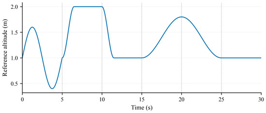
To examine continuous tracking, transition response, smooth trajectory change, and steady-state maintenance within a single simulation, a composite reference trajectory $r\left(t\right)$ consisting of six continuous subtasks was constructed. The first segment is sinusoidal tracking. The second segment rises smoothly from $1\mathrm{m}$ to $2\mathrm{m}$ during the first $1.5\mathrm{s}$ of the segment and then holds $2\mathrm{m}$ until $t=10\mathrm{s}$. The third segment similarly descends from $2\mathrm{m}$ to $1\mathrm{m}$ during the first $1.5\mathrm{s}$ and then holds $1\mathrm{m}$ until $t=15\mathrm{s}$. The fourth and fifth segments are full-segment raised-cosine transitions, and the sixth segment is constant-value holding. The transition parts are generated using a raised-cosine function to prevent reference discontinuities from dominating the response. The resulting six-segment reference trajectory, exported from the same profile-generation formula used in the simulations, is shown in Figure 1.

Figure 1. Exact six-segment composite reference trajectory used for training and testing. The curve is generated from the same profile formula used to construct the simulation input $h_{\mathrm{ref}}\left(t\right)$; the vertical dotted lines indicate the 5 s segment boundaries.

For reproducibility, define

$$\mathrm{rc}(t;t_0,T,y_0,y_1)=y_0+(y_1-y_0){\displaystyle \frac{1-\cos \left(\pi \mathrm{clip}\left((t-t_0)/T,0,1\right)\right)}{2}},$$

(9)

where $\mathrm{clip}(x,0,1)=\min \left(\max \right(x,0),1)$. With $h_0=1\mathrm{m}$, the exact reference trajectory is

$$r\left(t\right)=\left\{\begin{array}{cc}{h}_0+0.6\sin (2\pi t/5),\hfill & 0\le t<5,\hfill \\ h_0+\mathrm{rc}(t;5,1.5,0,1),\hfill & 5\le t<10,\hfill \\ h_0+1-\mathrm{rc}(t;10,1.5,0,1),\hfill & 10\le t<15,\hfill \\ \mathrm{rc}(t;15,5,1,1.8),\hfill & 15\le t<20,\hfill \\ \mathrm{rc}(t;20,5,1.8,1),\hfill & 20\le t<25,\hfill \\ 1,\hfill & 25\le t\le 30.\hfill \end{array}\right.$$

(10)

Let $y\left(t\right)$ be the plant output with the applied reference, control input, actuator saturation, and process-disturbance realization. During testing, the disturbance signal $w\left(t\right)$ was implemented as an equivalent vertical acceleration disturbance in the simulation profile, while $v\left(t\right)$ denotes additive measurement noise. The measured output used by the controller is

$$y_m\left(t\right)=y\left(t\right)+v\left(t\right).$$

(11)

The controller input error is defined as

$$e\left(t\right)=r\left(t\right)-y_m\left(t\right),$$

(12)

and the error change rate $ec\left(t\right)$ is approximated by a discrete difference. The process disturbance profile is generated as

$$w\left(t\right)={\kappa }_w\left[S\left(t\right){\displaystyle \sum _{i=1}^4}{a}_i\sin (2\pi f_{i}t+{\varphi }_i)+w_g\left(t\right)\right],$$

(13)

where

$$\left(f_i\right)=(0.30,0.80,1.50,2.50)\mathrm{Hz},\left(a_i\right)=(0.30,0.25,0.20,0.15).$$

(14)

The segment-dependent envelope is

$$S\left(t\right)=\left\{\begin{array}{cc}0.50,\hfill & 0\le t<10,\hfill \\ 0.65,\hfill & 10\le t<20,\hfill \\ 0.80,\hfill & 20\le t\le 30,\hfill \end{array}\right.$$

(15)

and the local gust is

$$w_g\left(t\right)=\left\{\begin{array}{cc}{\displaystyle \frac{A_g}{2}}\left[1-\cos \left(\pi (t-t_c)/W_g\right)\right],\hfill & |t-t_c|\le W_g,\hfill \\ 0,\hfill & \mathrm{otherwise},\hfill \end{array}\right.$$

(16)

with $t_c=17.5\mathrm{s}$, $W_g=0.60\mathrm{s}$, and $A_g=0.35\mathrm{m}/{\mathrm{s}}^2$. The baseline and strong-disturbance settings use ${\kappa }_w=0.25$ and ${\kappa }_w=1$, respectively. Measurement noise is generated as

$$v\left(t\right)={\displaystyle \sum _{j=1}^4}{b}_j\sin (2\pi f_j^{m}t+{\psi }_j),$$

(17)

where

$$\left(f_j^m\right)=(5.0,7.0,0.6,9.0)\mathrm{Hz},\left(b_j\right)=(0.006,0.006,0.004,0.003)\mathrm{m}.$$

(18)

For each seed, the phases ${\varphi }_i$ and ${\psi }_j$ were sampled from $[0,2\pi )$ using the Mersenne Twister generator. Thus, controllers were compared for the same realization within each seed, while different seeds provided different disturbance/noise phases.

The training seed set was fixed as

$${\mathcal{S}}_t=\{1201,1202,1203,1204,1205\},$$

(19)

and the independent Monte Carlo test set was

$${\mathcal{S}}_{\mathrm{test}}=\{1,2,\dots ,100\}.$$

(20)

The complete consecutive sequence 1–100 was fixed as the test set; seeds were not selected after observing controller performance. This prevents post hoc removal of unfavorable test realizations. For the same seed, all controllers shared exactly the same reference trajectory, process disturbance, and measurement-noise realization, thereby forming paired comparison samples. Monte Carlo simulation was used here as a numerical sampling procedure rather than as proof of robustness [31]. This design addresses seed-selection bias within the specified profile generator, but it does not establish robustness to other disturbance frequency sets or noise amplitudes.

For reproducibility, the seed-level archive recorded the controller-wise metrics and validity status for every test seed. Full scheduled-order, plant-output, and applied-input trajectories were retained for the representative traces used in the figures, rather than for every Monte Carlo run. The profile-generation function supplied in the Supplementary Materials deterministically reconstructs the reference, process disturbance, and measurement noise from a seed and accepts ${\kappa }_w$ as an explicit disturbance-scale parameter; its default value is ${\kappa }_w=0.25$, and the strong-disturbance data use the same phases and formula with ${\kappa }_w=1$. The main statistical tables in Section 4 were computed from the paired seed-level records.

3.2. Unified Fixed-Order and Variable-Order Fuzzy Fractional PID Structure

To keep the comparison controlled, both controllers were implemented within the same two-input five-output Sugeno fuzzy fractional-order PID framework. The difference was restricted to the additional scheduling mechanism for the integral and derivative orders; the VO controller therefore retained extra order-scheduling parameters, while the gain channels and the remaining numerical protocol were shared. The controller inputs are the error e and error change rate $ec$, while the outputs are $K_p,K_i,K_d,\alpha ,\beta$. In this paper, $\alpha$ denotes the fractional integral order and $\beta$ denotes the fractional derivative order. The unsaturated control output is

$$u_c\left(t\right)=K_p(e,ec)e\left(t\right)+K_i(e,ec)D^{-\alpha \left(t\right)}e\left(t\right)+K_d(e,ec)D^{\beta \left(t\right)}e\left(t\right).$$

(21)

The actual plant-side command is then obtained by saturation:

$$u\left(t\right)={\mathrm{sat}}_{[-12,25]}\left(u_c\left(t\right)\right).$$

(22)

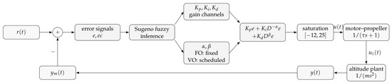
Figure 2 summarizes the unified FO/VO fuzzy FOPID structure. FO and VO share the same fuzzy gain channels and plant-side saturation; only the scheduling of $\alpha$ and $\beta$ differs.

Figure 2. Actuator-constrained unified FO/VO fuzzy fractional PID closed-loop structure. FO and VO share the same gain channels, fractional-order implementation, saturation, actuator, and plant; only the online scheduling of $\alpha$ and $\beta$ differs.

For the FO controller, $\alpha$ and $\beta$ are constant. For the VO controller, $\alpha \left(t\right)$ and $\beta \left(t\right)$ are scheduled online according to the closed-loop state. All controllers share the same normalized inputs, $7\times 7$ input-rule grid, gain-rule consequent index templates, and fractional-order numerical implementation. The following description focuses on the elements needed to reproduce the FO/VO comparison, with the FOPID and Sugeno foundations given in [1,4,5].

Before fuzzy inference, the physical error and error-change signals are processed as

$$\tilde{e}={\mathrm{sat}}_{[-1,1]}\left({\displaystyle \frac{{\mathcal{D}}_{0.01}\left(e\right)}{0.4}}\right),\widetilde{ec}={\mathrm{sat}}_{[-1,1]}\left({\displaystyle \frac{{\mathcal{D}}_{0.05}\left(ec\right)}{2.0}}\right),$$

(23)

where ${\mathcal{D}}_d\left(x\right)=0$ for $\left|x\right|<d$ and ${\mathcal{D}}_d\left(x\right)=x$ otherwise. Thus, the error and error-change dead zones are $0.01\mathrm{m}$ and $0.05\mathrm{m}/\mathrm{s}$, respectively. Seven triangular membership functions, labeled NB, NM, NS, ZO, PS, PM, and PB, are defined on each normalized input. Their final optimized parameters are not symmetric; the exact triples are reported in Appendix A.1.

The two inputs form a $7\times 7$ (49-rule) grid. For rule $(i,j)$, the product firing weight is

$$w_{ij}={\mu }_i^e\left(\tilde{e}\right){\mu }_j^{ec}\left(\widetilde{ec}\right).$$

(24)

The gain channels use the shared consequent-index templates in Appendix A. Their exact optimized singleton levels are also given in Appendix A.1. The FO stage uses this structured parameterization rather than searching 49 independent consequents for each output. The VO stage retains the optimized input membership functions and all gain-channel consequents and changes only the order consequents through four additional parameters.

Let ${\alpha }^{*}$ and ${\beta }^{*}$ denote the optimized FO orders, and let $\Delta {\alpha }_{ij}$ and $\Delta {\beta }_{ij}$ be the two integer-valued $7\times 7$ template matrices in Appendix A. The VO stage uses the four-dimensional vector

$$x_{\mathrm{VO}}=(g_{\alpha },{\delta }_{\alpha },g_{\beta },{\delta }_{\beta }),$$

(25)

and first computes a desired constant consequent for each rule:

$$a_{ij}^c={\alpha }^{*}+{\delta }_{\alpha }+0.1g_{\alpha }\Delta {\alpha }_{ij},$$

(26)

$$b_{ij}^c={\beta }^{*}+{\delta }_{\beta }+0.1g_{\beta }\Delta {\beta }_{ij}.$$

(27)

For the integral order, $a_{ij}^c$ is clipped to the intersection of $[0.5,1.3]$ and $[{\alpha }^{*}-0.2,{\alpha }^{*}+0.2]$. For the derivative order, $b_{ij}^c$ is clipped to the intersection of $[0.5,1.5]$ and $[{\beta }^{*}-0.5,{\beta }^{*}+0.3]$. Each clipped value is then mapped to the nearest singleton in $\mathcal{L}=\{0.5,0.6,\dots ,1.5\}$:

$$a_{ij}=Q_{0.1}\left(\mathrm{clip}\left(a_{ij}^c\right)\right),b_{ij}=Q_{0.1}\left(\mathrm{clip}\left(b_{ij}^c\right)\right).$$

(28)

Sugeno weighted-average inference produces the requested online orders

$${\alpha }_{\mathrm{req}}={\displaystyle \frac{{\sum }_{i,j}{w}_{ij}{a}_{ij}}{{\sum }_{i,j}{w}_{ij}}},{\beta }_{\mathrm{req}}={\displaystyle \frac{{\sum }_{i,j}{w}_{ij}{b}_{ij}}{{\sum }_{i,j}{w}_{ij}}}.$$

(29)

Although the rule consequents lie on a 0.1 grid, Equation (29) generally gives continuous requested values when several rules are active. The four optimization bounds are

$$g_{\alpha }\in [0,1.2],{\delta }_{\alpha }\in [-0.05,0.05],g_{\beta }\in [0,2.0],{\delta }_{\beta }\in [-0.15,0.15].$$

(30)

Equation (21) is the controller-design expression. In the numerical implementation, it is not evaluated through an exact variable-order differintegral. For a constant order $\gamma$ and zero initial conditions, the two fractional channels have the Laplace-domain representations

$$\mathcal{L}\left\{D^{-\gamma }e\left(t\right)\right\}=s^{-\gamma }E\left(s\right),\mathcal{L}\left\{D^{\gamma }e\left(t\right)\right\}=s^{\gamma }E\left(s\right).$$

(31)

Each constant-order operator is implemented in Simulink using the FOMCON fractional derivative or integrator block [32]. For an exponent $\nu$, the Oustaloup approximation has the form [33]

$$s^{\nu }\approx K_{\nu }{\displaystyle \prod _{k=-N}^N}{\displaystyle \frac{s+{\omega }_{k,\nu }^{\prime }}{s+{\omega }_{k,\nu }}},$$

(32)

where

$$\begin{array}{cc}\hfill {\omega }_{k,\nu }^{\prime }& ={\omega }_b{\left({\displaystyle \frac{{\omega }_h}{{\omega }_b}}\right)}^{{\displaystyle \frac{k+N+(1-\nu )/2}{2N+1}}},\hfill \\ \hfill {\omega }_{k,\nu }& ={\omega }_b{\left({\displaystyle \frac{{\omega }_h}{{\omega }_b}}\right)}^{{\displaystyle \frac{k+N+(1+\nu )/2}{2N+1}}},K_{\nu }={\omega }_h^{\nu }.\hfill \end{array}$$

(33)

The implemented settings are $N=5$, ${\omega }_b=0.1\mathrm{rad}/\mathrm{s}$, and ${\omega }_h=100\mathrm{rad}/\mathrm{s}$. Therefore, each approximation contains $2N+1=11$ first-order pole–zero factors. The reported results concern this finite-band rational realization, not an exact infinite-dimensional fractional operator.

The numerical implementation contains constant-order modules at the eleven levels in $\mathcal{L}$. An output guard initializes $(\alpha ,\beta )=(0.9,1.21)$ and retains the previous valid request if the new request is non-finite, outside $[0.5,1.5]$, or differs from the previous value by more than $0.09$ in one update. The selector then applies a $0.02$ hysteresis, a four-update minimum dwell, and a maximum order change of $0.02$ per update. Finally, it linearly blends the outputs of the two adjacent constant-order modules. Thus, the rule consequents and operator library have 0.1 spacing, but the delivered channel output is not selected by a hard nearest-level switch. These are numerical continuity safeguards, not a stability proof. Related work has treated bumpless implementation of scheduled FOPID controllers through finite-dimensional LPV approximations [34]. The interpolation and safeguards used here serve only as numerical continuity devices; no LPV continuity guarantee from that study is claimed. The archived Monte Carlo tables do not contain clipping or guard counters, so their population-level activation frequencies are not reported.

The compared controllers are defined in Table 2.

Table 2. Controller definitions and roles.

Symbol	Definition	Role
FO	Optimized fixed-order fuzzy fractional-order PID	Main baseline
VO	Variable-order controller optimized with the composite index J	Main method
VOITAE	Archived variable-order controller trained with $J_{\mathrm{ITAE}}$ from an earlier FO order template	Auxiliary historical comparator; not an objective-only ablation
$V{O}_{\mathrm{frozen}}$	VO orders frozen at the pooled median of Segment 6 in the training set	Test of fixed operating-point shift
$V{O}_{\mathrm{noShift}}$	VO order-consequent pattern recentered on FO, subject to the stated order bounds	Test of online variation shape

Controller provenance was established by SHA-256 comparison with the final FIS archive. The two historical VO filenames had become interchanged relative to their training objectives during a later file-organization step; the numerical parameters were not altered. The archived ITAE-trained FIS is compatible with the archived fixed-order template having $(\alpha ,\beta )=(0.8,1.3)$ but not with the final FO template having $(\alpha ,\beta )=(0.9,1.2)$ for the archived decoder and bounds. The two FO templates have identical input membership functions, gain-singleton libraries, and gain-rule consequents; they differ in their fixed-order consequents. Because no optimizer log remains that would establish an otherwise identical optimization run from the final FO template, VOITAE is retained only as an auxiliary historical comparator and is not interpreted as an objective-only ablation. Here, VO and VOITAE denote the files matched to the composite-J and ITAE training records, respectively, rather than to the later filenames. The source-filename mapping, checksums, template comparison, and a machine-readable export of all 49 final order-rule indices are provided in the Supplementary Materials.

FO and VO are the primary comparison controllers. VOITAE is reported only as the provenance-qualified historical comparator. $V{O}_{\mathrm{frozen}}$ and $V{O}_{\mathrm{noShift}}$ are used only for the counterfactual analysis. According to the pooled median of the archived Segment 6 order samples from training seeds 1201–1205,

$${\alpha }_{\mathrm{frozen}}=0.8703,{\beta }_{\mathrm{frozen}}=1.1834.$$

(34)

The fixed-order baseline is

$${\alpha }_{\mathrm{FO}}=0.9,{\beta }_{\mathrm{FO}}=1.2.$$

(35)

Therefore, the pooled Segment 6 median offsets removed in $V{O}_{\mathrm{noShift}}$ are

$$\Delta \alpha =-0.0297,\Delta \beta =-0.0166.$$

(36)

Each order singleton is recentered by subtracting the corresponding shift and is then clipped to the admissible interval $[0.5,1.5]$. This setting allows Section 4 to compare a fixed operating-point shift with the retained online order-variation shape. It is a pair of counterfactual comparisons, not a complete causal decomposition.

3.3. Composite Performance Index and Two-Stage PSO Optimization

A single error-integral index does not separately characterize continuous tracking, transition quality, steady-state maintenance, and control variation in this composite task. Therefore, a composite performance index J aligned with the six-segment task was constructed. For the k-th segment, the base cost is defined as

$$J_k^{\mathrm{base}}=0.50nITA{E}_k+0.10nITS{E}_k+0.25nPo{s}_k+0.10\varphi \left(nYh{p}_k\right)+0.05\varphi \left(nUr{t}_k\right),$$

(37)

where $nITA{E}_k$ and $nITS{E}_k$ are task-scaled error terms, $nPo{s}_k$ describes peak deviation, $nYh{p}_k$ describes high-frequency output behavior, $nUr{t}_k$ describes control-variation intensity, and $\varphi (·)$ is a truncation-compression function. Performance evaluation is computed using the true output error, whereas the online controller input uses the measurement-noise-contaminated error $e\left(t\right)$. This separation prevents the injected measurement signal from entering the evaluation error directly.

Let segment k have local time $\tau =t-t_{k,0}$, length $L_k$, reference $r_k\left(t\right)$, output $y_k\left(t\right)$, input $u_k\left(t\right)$, and true error $e_k\left(t\right)=r_k\left(t\right)-y_k\left(t\right)$. The local reference scale is

$$A_k=\max \left(|r_k\left(t_{k,1}\right)-r_k\left(t_{k,0}\right)|,\underset{t}{\max }\left|r_k\left(t\right)\right|,1\right).$$

(38)

The task-scaled error terms are

$$nITA{E}_k={\displaystyle \frac{{\int }_0^{L_k}\tau \left|e_k\left(\tau \right)\right|d\tau }{A_k{L}_k+ϵ}},nITS{E}_k={\displaystyle \frac{{\int }_0^{L_k}\tau e_k^2\left(\tau \right)d\tau }{A_k^2{L}_k+ϵ}}.$$

(39)

For the one-sided peak-deviation term $nPo{s}_k$, the implementation first selects samples at which the response lies beyond the final segment level in the direction of the segment change and then trapezoidally integrates $\tau |r_k-y_k|$ over those selected sample times. The term is set to zero when the final amplitude change is at most $0.05\mathrm{m}$. For the high-frequency term, a $0.10\mathrm{s}$ moving average is subtracted from $y_k$ and

$$nYh{p}_k={\displaystyle \frac{\mathrm{var}(y_k-\mathrm{movmean}(y_k,0.10\mathrm{s}))}{A_k^2+ϵ}}.$$

(40)

For the control-variation term,

$$nUr{t}_k={\displaystyle \frac{{\int }_0^{L_k}{\left(\frac{d{u}_k}{dt}\right)}^{2}d\tau }{A_k^2+ϵ}}.$$

(41)

The compression function used for the high-frequency and control-variation terms is

$${\varphi }_c\left(x\right)=\sqrt{\min (x,c)},$$

(42)

with $c=10$ for $nYh{p}_k$ and $c=100$ for $nUr{t}_k$, and $ϵ$ denotes a small positive number used only to avoid division by zero. The final segment cost is

$$J_k=J_k^{\mathrm{base}}\exp \left({\displaystyle \frac{\max (0,e_{k,\max }-0.12)}{0.12}}\right),e_{k,\max }=\underset{t}{\max }\left|e_k\left(t\right)\right|.$$

(43)

The six segment weights are

$$({\omega }_1,\dots ,{\omega }_6)=(1.2,1.5,1.5,1.5,1.5,1.0),$$

(44)

and the final cost is aggregated as

$$J={\displaystyle \frac{{\sum }_{k=1}^6{\omega }_k{J}_k}{{\sum }_{k=1}^6{\omega }_k}}.$$

(45)

The exponential multiplier exceeds one only when the local maximum absolute error is greater than $0.12\mathrm{m}$. Because this multiplier can dominate tail values with strong disturbance, the strong-disturbance analysis also reports ITAE, peak deviation, positive-limit near-saturation ratio, in-band ratio, and control-input indicators. The weights and threshold are fixed design choices for this benchmark; their sensitivity is not evaluated here.

The archived ITAE-trained comparator uses an ITAE-centered objective $J_{\mathrm{ITAE}}$. To maintain the same segment division, scaling, and weighting protocol, this objective does not use a raw time-domain ITAE. Instead, the six local scaled ITAE terms are aggregated using the same segment weights:

$$J_{\mathrm{ITAE}}={\displaystyle \frac{{\sum }_{k=1}^6{\omega }_{k}nITA{E}_k}{{\sum }_{k=1}^6{\omega }_k}}.$$

(46)

$J_{\mathrm{ITAE}}$ corresponds to the main error-accumulation term in J, not a second independent evaluation system. The archived ITAE-trained controller is numerically close to VO in the reported tests. That proximity cannot isolate the effect of the objective, however, because its fixed-order template differs from the final FO template as described above. The counterfactual analysis therefore focuses on the provenance-consistent FO–VO pair, while objective-weight sensitivity remains unevaluated.

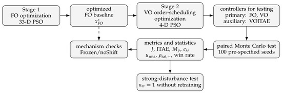
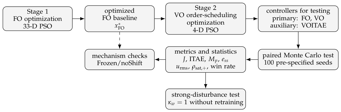
To limit the additional tuning freedom of the VO comparison, a two-stage PSO framework was adopted. In the first stage, FO fuzzy FOPID is tuned to obtain a fixed-order baseline. In the second stage, all other optimized FO parameters are kept unchanged, and only four VO-related incremental parameters are optimized. The FO stage optimizes a 33-dimensional structured parameter vector $x_{\mathrm{FO}}$, whereas the VO stage adds the four-dimensional adjustment vector $x_{\mathrm{VO}}$. This design does not remove the effect of the extra scheduling parameters, but it prevents the gain channels and membership functions from being retuned simultaneously with them. The simulation-based objective is non-convex and includes clipping and failure penalties; PSO is therefore used as a stochastic search heuristic, not as a certificate of global optimality. Genetic algorithms are a relevant alternative for this class of system-engineering optimization problem [35]. The present study does not claim that its reported controller is invariant to PSO restart or training-set choice; instead, the optimizer protocol was fixed, and the resulting controllers were tested on an independent paired 100-seed set. The complete optimization and paired testing protocol is illustrated in Figure 3.

Figure 3. Two-stage PSO optimization and paired Monte Carlo protocol. The final FO controller is optimized first; the primary VO controller then optimizes only the low-dimensional order-scheduling parameters. The provenance-qualified historical VOITAE controller is retained as an auxiliary comparator. The solid arrows denote the sequential optimization, testing, and analysis workflow; the dashed arrow denotes the direct use of the optimized FO baseline in the Frozen/noShift mechanism checks. The existing controllers are subsequently examined by paired tests, two FO–VO counterfactual order variants, and a strong-disturbance test without retraining.

The optimization problems are

$$x_{\mathrm{FO}}^{*}=\arg \underset{x_{\mathrm{FO}}\in {\Omega }_{\mathrm{FO}}}{\min }{\displaystyle \frac{1}{|{\mathcal{S}}_t|}}\sum _{s\in {\mathcal{S}}_t}{J}^{\left(s\right)}\left(x_{\mathrm{FO}}\right),$$

(47)

$$x_{\mathrm{VO}}^{*}=\arg \underset{x_{\mathrm{VO}}\in {\Omega }_{\mathrm{VO}}}{\min }{\displaystyle \frac{1}{|{\mathcal{S}}_t|}}\sum _{s\in {\mathcal{S}}_t}{J}^{\left(s\right)}(x_{\mathrm{FO}}^{*},x_{\mathrm{VO}}),$$

(48)

The archived ITAE training script applies the analogous four-dimensional search with $J_{\mathrm{ITAE}}$, but its retained final FIS is tied to the earlier fixed-order template described above. It is therefore not written as an objective-only optimization conditional on the final $x_{\mathrm{FO}}^{*}$. If premature simulation termination, NaN/Inf values, divergence, or other numerical abnormalities occur, a preset large penalty is returned. The standard PSO update equations and parameter settings are provided in Appendix A.4.

3.4. Implementation Constraints and Numerical Protection

Because the online variable-order fuzzy FOPID controller involves fuzzy inference, fractional-order operator approximation, and order scheduling, numerical safeguards were applied identically in training and testing. First, the plant-side equivalent input was clipped to $[-12,25]$. This is a common numerical bound for the comparison, not a physical actuator-identification claim. Second, $\alpha \left(t\right)$ and $\beta \left(t\right)$ were restricted and interpolated as specified above for all VO-related controllers. Third, the order-output guard retained the preceding valid order after a non-finite, out-of-range, or excessively discontinuous order request. This guard concerns the two order channels; it is distinct from the objective-function penalty. Finally, a preset large objective value was assigned only when a trial simulation terminated prematurely, diverged numerically, produced non-finite outputs, or exceeded the stated engineering output bounds.

All reported simulations used the MATLAB/Simulink R2023b model with the variable-step stiff solver ode23tb, maximum step size $0.002\mathrm{s}$, relative tolerance ${10}^{-3}$, and absolute tolerance ${10}^{-4}$. The profile generator supplied the reference, disturbance, and measurement-noise signals on a uniform $0.002\mathrm{s}$ grid. For failed simulations, non-finite outputs, premature termination, or outputs exceeding the engineering protection bounds, the objective function returned a large penalty rather than a numerical performance value. These treatments do not constitute a formal stability proof, but they ensure that the controllers are trained and tested with the same numerical implementation constraints and prevent numerical abnormalities from being misinterpreted as control-mechanism benefits.

3.5. Testing Metrics and Statistical Protocol

In the testing stage, FO, VO, VOITAE, and the two counterfactual controllers were evaluated on the independent 100-seed test set. The main index is J. Auxiliary measures are $J_{\mathrm{ITAE}}$, maximum normalized overshoot $M_p$, robust settling time $T_{s,\mathrm{robust}}$, steady-state error $e_{ss}$, and total in-band ratio ${\rho }_{\mathrm{inband},\mathrm{total}}$. For segments with a final amplitude change greater than $0.05\mathrm{m}$, $M_p$ is the maximum segment-wise directional overshoot of the $0.10\mathrm{s}$ moving-average output, normalized by the segment amplitude. The reported $e_{ss}$ is the absolute mean filtered true error over the final 30% of Segment 6. The input-side conclusions use the RMS applied input $u_{\mathrm{rms}}$ and the positive-limit near-saturation ratio ${\rho }_{\mathrm{sat},+}$; the archive also retains input-percentile and unsaturated-command diagnostics, but they are not used to extend the main claim. Here $u_{\mathrm{rms}}={\left[T^{-1}{\int }_0^T{u}^2\left(t\right)dt\right]}^{1/2}$ was evaluated by time integration, rather than by an unweighted mean over the output rows of the variable-step solver. These measures were examined together so that a lower error index is not interpreted without its associated input behavior.

The in-band and robust-settling metrics were computed from a low-pass filtered true error. The error band is

$${\epsilon }_{\mathrm{band}}=\min \left(\max (0.02\Delta r,2{\sigma }_n),\min (0.05\Delta r,0.06)\right),$$

(49)

where $\Delta r={\max }_{t}r\left(t\right)-{\min }_{t}r\left(t\right)$ and ${\sigma }_n$ is estimated from the high-frequency residual of the last segment after a $0.5\mathrm{s}$ moving-average detrending. The low-pass time constant is $0.2\mathrm{s}$. The total in-band ratio is the time fraction for which the filtered true error lies within $\pm {\epsilon }_{\mathrm{band}}$. The robust settling time was computed segment-wise for Segments 2–6. It uses a $1.0\mathrm{s}$ sliding window, a 95% in-band probability criterion, a $1.0\mathrm{s}$ hold requirement, and a $0.2\mathrm{s}$ ignored interval after each segment start. The reported $T_{s,\mathrm{robust}}$ is the maximum of the segment values. Because the net-thrust saturation interval is asymmetric, the archived near-saturation metric is defined as the positive-limit time fraction ${\rho }_{\mathrm{sat},+}$ for which $u\left(t\right)\ge 0.99U_{\max }$ with $U_{\max }=25$. It is therefore interpreted as exposure to the upper net-thrust limit, not as a two-sided total saturation-time ratio.

This paper does not use a single J value as the sole basis for drawing conclusions. Instead, the interpretation considers improvement in the main index, possible degradation in auxiliary metrics, and changes in the two pre-specified input indicators. If a controller improves J but produces much larger RMS input, stronger upper-limit exposure, or worse steady-state maintenance, the result is not treated as a favorable trade-off in this benchmark.

The statistical results are reported using mean, standard deviation, median, paired mean difference with a percentile-bootstrap 95% confidence interval, Wilcoxon signed-rank test [36], and per seed win rate. Since all controllers share the same reference trajectory, process disturbance, and measurement-noise realization with the same seed, the comparison is paired. Representative samples were selected according to the distribution of the relative improvement of VO over FO in the main index J, while the sample interpretation also considers segment-level errors, in-band ratio, and control-input behavior.

4. Results and Numerical Discussion

This section reports the results under the protocol in Section 3. It considers the composite index together with error accumulation, in-band behavior, applied-input magnitude, and ${\rho }_{\mathrm{sat},+}$. Three questions are examined: whether the paired VO distribution differs from FO; whether the difference is more consistent with online order variation than with greater applied-input magnitude, positive-limit exposure, or a fixed-order shift; and whether a similar pattern appears in the existing strong-disturbance test.

4.1. Training Results and Baseline Monte Carlo Statistics

The archived controllers were evaluated on the common five-seed training set in Table 3. FO and VO form the provenance-consistent two-stage optimization pair. VOITAE is shown for completeness but retains the earlier fixed-order template described in Section 3.

Table 3. Evaluation of the retained controller files on the five training seeds. VOITAE is a provenance-qualified historical comparator, not an objective-only ablation from the final FO template.

Controller	J Mean	ITAE Mean	${\mathit{M}}_{\mathit{p}}$ Mean	${\mathit{T}}_{\mathit{s},\mathbf{robust}}$ Mean	${\mathit{\rho }}_{\mathbf{sat},+}$ Mean	${\mathit{\rho }}_{\mathbf{inband},\mathbf{total}}$ Mean
init	0.9744	0.08350	0.23205	3.4096	0.00036	0.6911
FO	0.6418	0.06374	0.10791	2.4760	0.00546	0.8388
VO	0.6064	0.05914	0.11193	2.7352	0.00317	0.8970
VOITAE	0.6062	0.05913	0.11193	2.7352	0.00318	0.8972

Relative to the initial controller, FO reduces the five-seed mean of J from 0.9744 to 0.6418, lowers ITAE, $M_p$, and robust settling time, and increases the in-band ratio. Its positive-limit near-saturation ratio rises from 0.00036 to 0.00546, so the training table does not show across-metric dominance. VO further reduces J, ITAE, and positive-limit exposure relative to FO and increases the in-band ratio, while the training-set means of $M_p$ and robust settling time do not improve further. VOITAE gives nearly identical numerical values, but the template mismatch prevents attributing that proximity solely to the two objective functions.

Under the baseline disturbance condition ${\kappa }_w=0.25$, FO, VO, and VOITAE were evaluated on the 100 pre-specified distinct test seeds. The controllers share the same reference trajectory, process disturbance, and measurement-noise realization with the same seed. Therefore, the comparison is strictly paired. Table 4 gives the compressed core statistics.

Table 4. Core statistics of FO and VO under the baseline disturbance condition ${\kappa }_w=0.25$.

Metric	FO Mean	VO Mean	Relative Change	p-Value	Win Rate
J	0.6157	0.5913	$-3.97\%$	$4.53\times {10}^{-18}$	0.99
ITAE	0.06293	0.05849	$-7.06\%$	$3.90\times {10}^{-18}$	1.00
$M_p$	0.11218	0.11313	$+0.85\%$	0.970	0.62
$T_{s,\mathrm{robust}}$	2.5901	2.4938	$-3.72\%$	0.251	0.64
$e_{ss}$	0.03684	0.02298	$-37.62\%$	$4.02\times {10}^{-18}$	0.99
$u_{\mathrm{rms}}$	8.8043	8.5242	$-3.18\%$	$3.90\times {10}^{-18}$	1.00
${\rho }_{\mathrm{sat},+}$	0.00698	0.00395	$-43.36\%$	$1.33\times {10}^{-17}$	0.94
${\rho }_{\mathrm{inband},\mathrm{total}}$	0.8547	0.9128	$+6.80\%$	$3.90\times {10}^{-18}$	1.00

To distinguish magnitude from statistical significance, Table 5 reports paired mean differences and 95% percentile-bootstrap confidence intervals (10,000 resamples; random seed 20260804). The intervals exclude zero for J, ITAE, $e_{ss}$, $u_{\mathrm{rms}}$, ${\rho }_{\mathrm{sat},+}$, and ${\rho }_{\mathrm{inband},\mathrm{total}}$ but not for $M_p$ or $T_{s,\mathrm{robust}}$.

Table 5. Paired effect sizes for VO relative to FO under the baseline condition. Differences are VO minus FO; a negative value favors VO except for ${\rho }_{\mathrm{inband},\mathrm{total}}$.

Metric	Mean Difference	Bootstrap 95% CI	VO-Favorable Seeds
J	$-0.02443$	$[-0.02694,-0.02192]$	99/100
ITAE	$-0.00445$	$[-0.00484,-0.00407]$	100/100
$M_p$	$+0.00095$	$[-0.00033,0.00230]$	62/100
$T_{s,\mathrm{robust}}$ (s)	$-0.09630$	$[-0.28817,0.08838]$	64/100
$e_{ss}$ (m)	$-0.01386$	$[-0.01453,-0.01319]$	99/100
$u_{\mathrm{rms}}$ (N)	$-0.28011$	$[-0.28979,-0.27018]$	100/100
${\rho }_{\mathrm{sat},+}$	$-0.00302$	$[-0.00352,-0.00255]$	94/100
${\rho }_{\mathrm{inband},\mathrm{total}}$	$+0.05810$	$[0.05286,0.06319]$	100/100

Table 6 reports the corresponding 100-seed mean statistics for the primary controllers, the historical ITAE-trained comparator, and the two mechanism counterfactuals under the same baseline disturbance condition. This expanded view is useful for interpreting the compact FO–VO comparison in Table 4.

Table 6. Expanded 100-seed mean statistics under the baseline disturbance condition ${\kappa }_w=0.25$. VOITAE is the provenance-qualified historical comparator and is not an objective-only ablation.

Controller	J	ITAE	${\mathit{M}}_{\mathit{p}}$	${\mathit{T}}_{\mathit{s},\mathbf{robust}}$	${\mathit{e}}_{\mathit{ss}}$	${\mathit{u}}_{\mathbf{rms}}$	${\mathit{\rho }}_{\mathbf{inband},\mathbf{total}}$
FO	0.61569	0.06293	0.11218	2.59012	0.03684	8.80429	0.85466
VO	0.59126	0.05849	0.11313	2.49382	0.02298	8.52419	0.91276
VOITAE	0.59126	0.05849	0.11313	2.49388	0.02298	8.52421	0.91276
$V{O}_{\mathrm{frozen}}$	0.60986	0.06188	0.11194	2.56237	0.03364	8.61057	0.87472
$V{O}_{\mathrm{noShift}}$	0.59389	0.05883	0.11277	2.47126	0.02541	8.70770	0.90052

Two observations follow from Table 6. First, VO and VOITAE are numerically close, but that observation cannot establish equivalence of the two training objectives because the retained controllers do not share the same fixed-order template. Second, the relative positions of $V{O}_{\mathrm{noShift}}$ and $V{O}_{\mathrm{frozen}}$ provide an initial, restricted comparison of the retained scheduling pattern and the constant-order alternative. This comparison is quantified in the subsequent mechanism-analysis section.

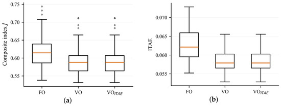
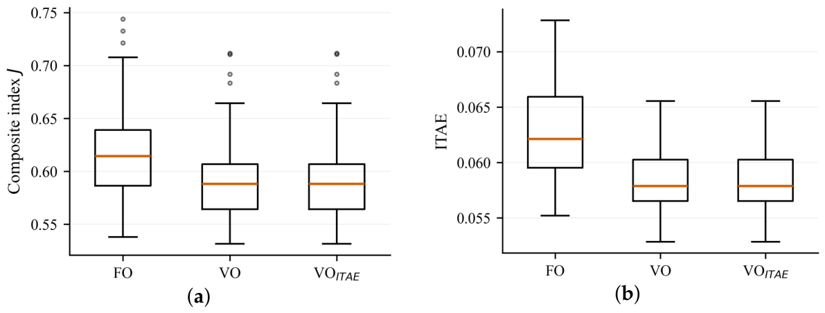
Figure 4 further visualizes the paired-test distributions of the two dominant error-related metrics, J and ITAE. The role of this figure is statistical rather than trajectory-level: panel (a) checks whether the main composite index shifts in the paired 100-seed test, while panel (b) checks whether the dominant error-accumulation term exhibits the same trend. Showing the two panels together avoids presenting the composite-index improvement without its main error-integral counterpart. The boxplots are consistent with the statistics in Table 4: the downward shift from FO to VO is visible across the paired distribution and is not confined to isolated samples.

Figure 4. Distributions of the main error-related metrics over 100 paired test seeds under the baseline disturbance condition: (a) composite performance index J; (b) ITAE.

In terms of the main index, VO reduces the mean value of J from 0.6157 to 0.5913, corresponding to a 3.97% reduction. The paired mean difference is $-0.02443$ (95% CI $[-0.02694,-0.02192]$). ITAE decreases from 0.06293 to 0.05849, with a paired mean difference of $-0.00445$ (95% CI $[-0.00484,-0.00407]$). For steady-state and constraint-related indicators, $e_{ss}$ decreases by 37.62%, the positive-limit near-saturation ratio decreases by 43.36%, and the in-band ratio increases by 6.80%. The RMS input decreases by 3.18%. In contrast, the confidence intervals for $M_p$ and $T_{s,\mathrm{robust}}$ include zero. Thus, the evidence supports a moderate distribution-level improvement in the stated error, in-band, and pre-specified input indicators; it does not support comprehensive superiority in every transient metric.

For J, ITAE, $e_{ss}$, ${\rho }_{\mathrm{sat},+}$, $u_{\mathrm{rms}}$, and ${\rho }_{\mathrm{inband},\mathrm{total}}$, the signed-rank results are consistent with a directional shift in the paired differences. The corresponding per seed win counts show the same direction. Neither result measures effect magnitude or proves that a mean is unaffected by extreme values; magnitude is reported separately by the paired mean differences and confidence intervals. A win count is also not an estimate of operational-success probability. For $M_p$ and $T_{s,\mathrm{robust}}$, the confidence intervals include zero and the signed-rank tests do not reject the null hypothesis at the 0.05 level. VO is therefore not interpreted as dominating FO in all transient metrics; the observed difference is limited to the reported composite, error, in-band, and input indicators.

Under the baseline condition, VOITAE and VO are nearly identical in the training-seed and test summaries. This numerical proximity does not show whether the extra peak, high-frequency, and control-variation terms affected optimization, because the retained ITAE-trained controller used an earlier fixed-order template. The objective-only comparison is therefore withdrawn, and sensitivity to other weight choices remains unevaluated.

4.2. Representative Samples and Local Behavior

Overall statistics reveal distributional trends, but they do not show how the benefit appears for different realizations. To avoid subjective sample selection, three representative seeds were selected according to the distribution of the relative improvement of VO over FO in the main index J: a median-improvement seed, a minimum-improvement seed, and a maximum-improvement seed. The results are shown in Table 7.

Table 7. Representative samples selected according to the relative improvement in J under the baseline condition.

Seed	${\mathit{J}}_{\mathbf{FO}}$	${\mathit{J}}_{\mathbf{VO}}$	Relative Improvement	Type
6	0.6395	0.6142	3.96%	Median improvement
55	0.6076	0.6095	$-0.32\%$	Minimum improvement
100	0.6553	0.6004	8.39%	Maximum improvement

For seed 6, the relative improvement is 3.96%, close to the mean improvement. Seed 55 is the most unfavorable case, where J for VO is 0.32% higher than that for FO. Seed 100 gives the largest observed improvement, with an 8.39% reduction in J. These cases show the range of paired outcomes; the largest improvement is not treated as a typical operating case.

Although the representative samples were selected according to J, their interpretation is not limited to J. For the maximum-improvement sample, seed 100, the in-band ratio increases by 32.08% in Segment 5 and by 29.56% in Segment 6. These two values show that the difference within this selected trace is not uniform across the task; they do not establish a population-level segment mechanism. The full saved trajectory records for the representative seeds are included in the Supplementary Materials. They are not used as main-text evidence under the baseline condition because the FO, VO, and VOITAE altitude curves overlap strongly at the full 30 s scale and do not reveal the distribution-level differences as clearly as the paired statistics.

4.3. Control Input and Counterfactual Analysis

Output-performance improvement alone is insufficient to establish a favorable trade-off, because a larger control input can also reduce tracking error. The time-weighted RMS applied input and positive-limit near-saturation ratio were therefore examined together with the selected input histories. The results show that $u_{\mathrm{rms}}$ of VO is lower than that of FO for seeds 6, 55, and 100. The time-weighted FO/VO $u_{\mathrm{rms}}$ values for these three samples are 8.4966/8.2419, 8.5026/8.2459, and 8.4876/8.2619, respectively. This agrees with the paired statistics of $u_{\mathrm{rms}}$ and ${\rho }_{\mathrm{sat},+}$ in Table 4: the two pre-specified input indicators do not increase for VO. Because ${\rho }_{\mathrm{sat},+}$ measures only positive upper-limit exposure, this evidence does not establish a reduction in total two-sided saturation time. Within this limited input-side evidence, the result is more consistent with redistribution of closed-loop dynamics by online order scheduling than with a higher RMS input or greater positive-limit exposure.

Two counterfactual controllers, $V{O}_{\mathrm{frozen}}$ and $V{O}_{\mathrm{noShift}}$, were used to examine the fixed-order-shift explanation. $V{O}_{\mathrm{frozen}}$ fixed the VO orders at the pooled median of Segment 6 in the training set. $V{O}_{\mathrm{noShift}}$ retained the VO consequent pattern but recentered its order singletons on FO, with the stated admissible-order clipping applied. The results are shown in Table 8.

Table 8. Counterfactual retention ratios based on paired mean values of J. For counterfactual C, the ratio is $({\overline{J}}_{\mathrm{FO}}-{\overline{J}}_C)/({\overline{J}}_{\mathrm{FO}}-{\overline{J}}_{\mathrm{VO}})$ on the common valid seeds for that comparison. The two ratios are separate and are not additive shares.

Condition	Frozen Valid Pairs	Frozen Ratio	noShift Valid Pairs	noShift Ratio
${\kappa }_w=0.25$	100	23.9%	100	89.2%

Under the baseline condition, both counterfactuals used all 100 pre-specified test seeds. The two ratios were restricted comparisons, not percentages of mutually exclusive causal sources. The strong-condition counterfactuals in the earlier archive were derived from the file identified by the provenance audit as the ITAE-centered controller. They are therefore excluded rather than used to make a mechanism claim about the composite-J VO. Within the corrected baseline protocol, the relative positions of the two counterfactuals were used only to assess which of the two stated explanations is more consistent with the observed mean difference.

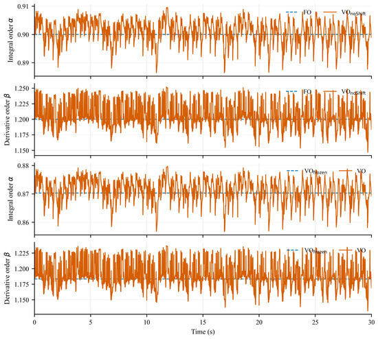
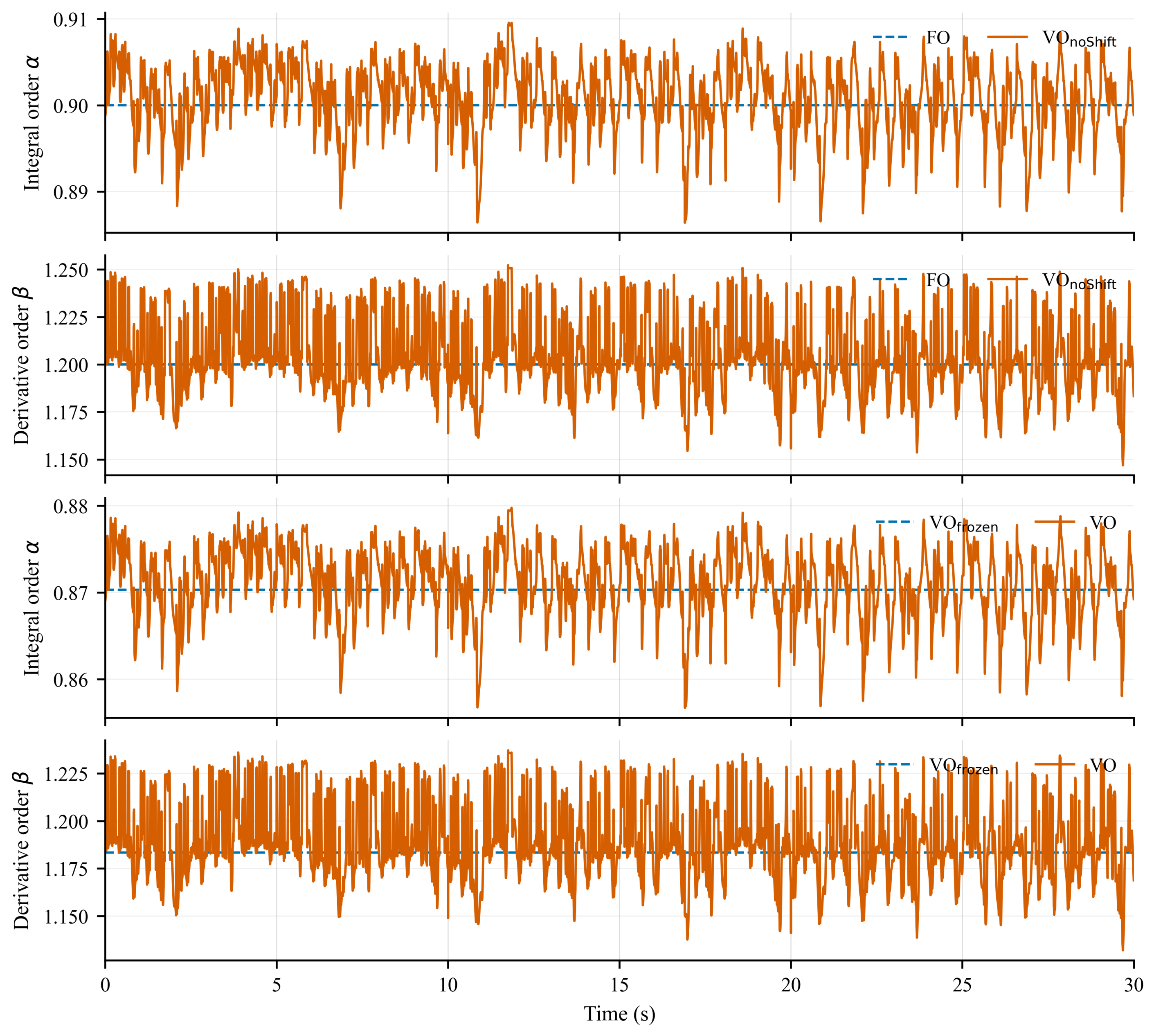
The order trajectories provide an intuitive supplement to the mechanism table. A single-axis overlay of $\alpha \left(t\right)$ and $\beta \left(t\right)$ is visually crowded because the two orders occupy different value ranges and the $\beta$ trajectories overlap heavily. Therefore, Figure 5 uses a four-panel layout: the first two panels compare FO with $V{O}_{\mathrm{noShift}}$, and the last two panels compare $V{O}_{\mathrm{frozen}}$ with VO. This layout separates the integral and derivative orders and makes the constant-order references and online order variation easier to read. For the displayed median-improvement baseline trace (seed 6), VO gives $\alpha \in [0.8567,0.8797]$ and $\beta \in [1.1320,1.2371]$, which lie strictly inside the corresponding admissible intervals. The absolute excursions are therefore modest, particularly for $\alpha$. The point of the extra scheduling stage is not that it generates large order excursions but that the Frozen/noShift counterfactuals test whether the observed time variation is distinguishable from a fixed-order shift under this numerical protocol. This is a mechanism result for the present approximation and order library; it is not evidence that every variable-order implementation or resolution will have the same relevance. Runtime and embedded-computation overhead were not measured, so the numerical difference is not presented as a demonstrated implementation-level cost advantage.

Figure 5. Representative order trajectories for the median-improvement seed. The four-panel layout separates $\alpha$ and $\beta$ and distinguishes the FO–noShift and Frozen–VO comparisons. The fixed-order and frozen-order curves are constant references, whereas the VO and noShift curves preserve state-dependent order variation. The figure illustrates the scheduling mechanism and is not used as an additional performance metric.

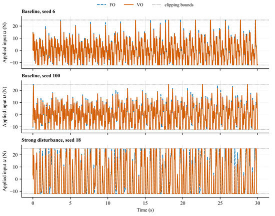
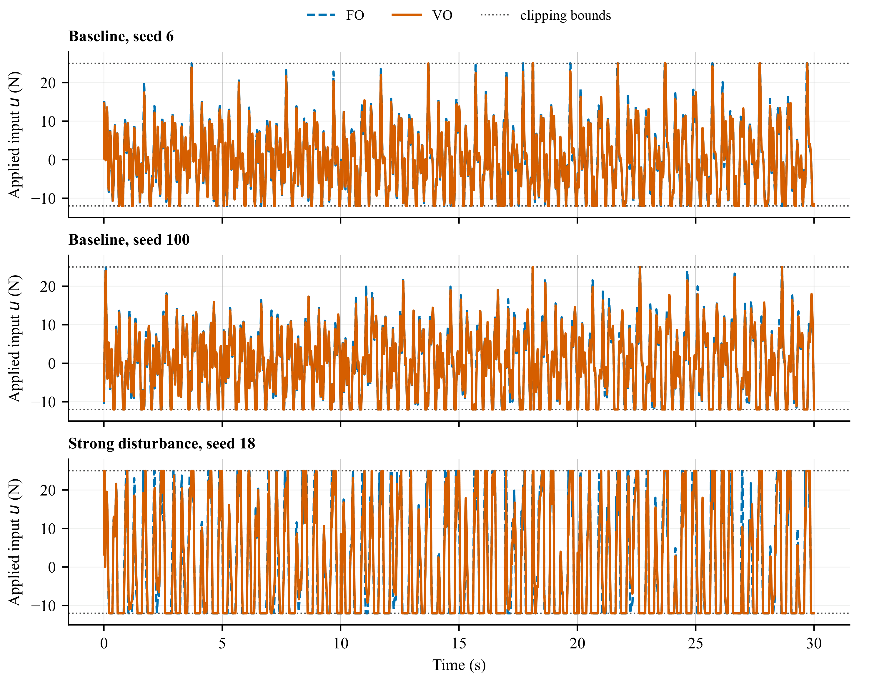
For transparency, Figure 6 provides the archived FO/VO input histories for two baseline seeds and one strong-disturbance seed. These traces are supplementary visual diagnostics rather than additional population-level evidence; the distributional input conclusion remains the paired analysis in Table 4 and Table 5. The dashed lines show the numerical clipping interval. In particular, the lower line represents near-complete thrust unloading in the reduced model and is not combined with ${\rho }_{\mathrm{sat},+}$ into a total saturation statistic.

Figure 6. Archived applied equivalent net-thrust inputs for representative paired FO/VO traces: baseline seeds 6 and 100, and strong-disturbance seed 18. The dashed lines are the common numerical clipping bounds. These selected traces illustrate input evolution; all population-level comparisons use the 100-seed paired statistics.

4.4. Persistence Under Strong-Disturbance Condition

The existing strong-disturbance test increased the process-disturbance scale to ${\kappa }_w=1$ without re-optimizing any controller. All controllers used the same test seeds and disturbance phases as in the baseline test. The value of J becomes large in some tail cases because its maximum-error term includes an exponential penalty. The archived tables do not contain a separate per seed flag for this term, so its exact activation count cannot be reconstructed without an instrumented rerun. For this reason, J is considered together with ITAE, peak deviation, positive-limit near-saturation ratio, in-band ratio, and applied-input measures. This test concerns persistence across two disturbance intensities with the same frequency set; it is not a retrained optimum or a test of other disturbance spectra. Core FO–VO summary statistics are reported in Table 9.

Table 9. Core statistics of FO and VO under the strong-disturbance condition ${\kappa }_w=1$.

Metric	FO Mean	VO Mean	Relative Change
J	1745.68	646.85	$-62.95\%$
ITAE	0.55225	0.43951	$-20.41\%$
$M_p$	0.88670	0.78272	$-11.73\%$
${\rho }_{\mathrm{sat},+}$	0.08742	0.06786	$-22.38\%$
${\rho }_{\mathrm{inband},\mathrm{total}}$	0.0654	0.1329	$+103.10\%$
$u_{\mathrm{rms}}$	14.0013	13.5141	$-3.48\%$

The corresponding all-controller strong-disturbance means are given in Table 10. Since no controller was retrained, this table is a persistence and degradation test rather than a new optimum for ${\kappa }_w=1$.

Table 10. Mean statistics under the strong-disturbance condition ${\kappa }_w=1$ without retraining. FO, VO, and VOITAE each had 100 valid runs. Counterfactual rows from the earlier archive are not included because they were derived from the file identified by the provenance audit as the ITAE-centered controller.

Controller	Valid n	J	ITAE	${\mathit{M}}_{\mathit{p}}$	${\mathit{e}}_{\mathit{ss}}$	${\mathit{u}}_{\mathbf{rms}}$	${\mathit{\rho }}_{\mathbf{inband},\mathbf{total}}$
FO	100	1745.68	0.55225	0.88670	0.40947	14.00133	0.06541
VO	100	646.85	0.43951	0.78272	0.31180	13.51409	0.13286
VOITAE	100	629.64	0.43961	0.78112	0.31257	13.51487	0.13291

Table 10 retains the primary VO controller and the historical ITAE-trained comparator because both are exact retained files and both have valid results for all 100 seeds. The strong test was used only as a no-retraining persistence check; it was not used for the corrected counterfactual mechanism comparison.

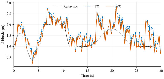
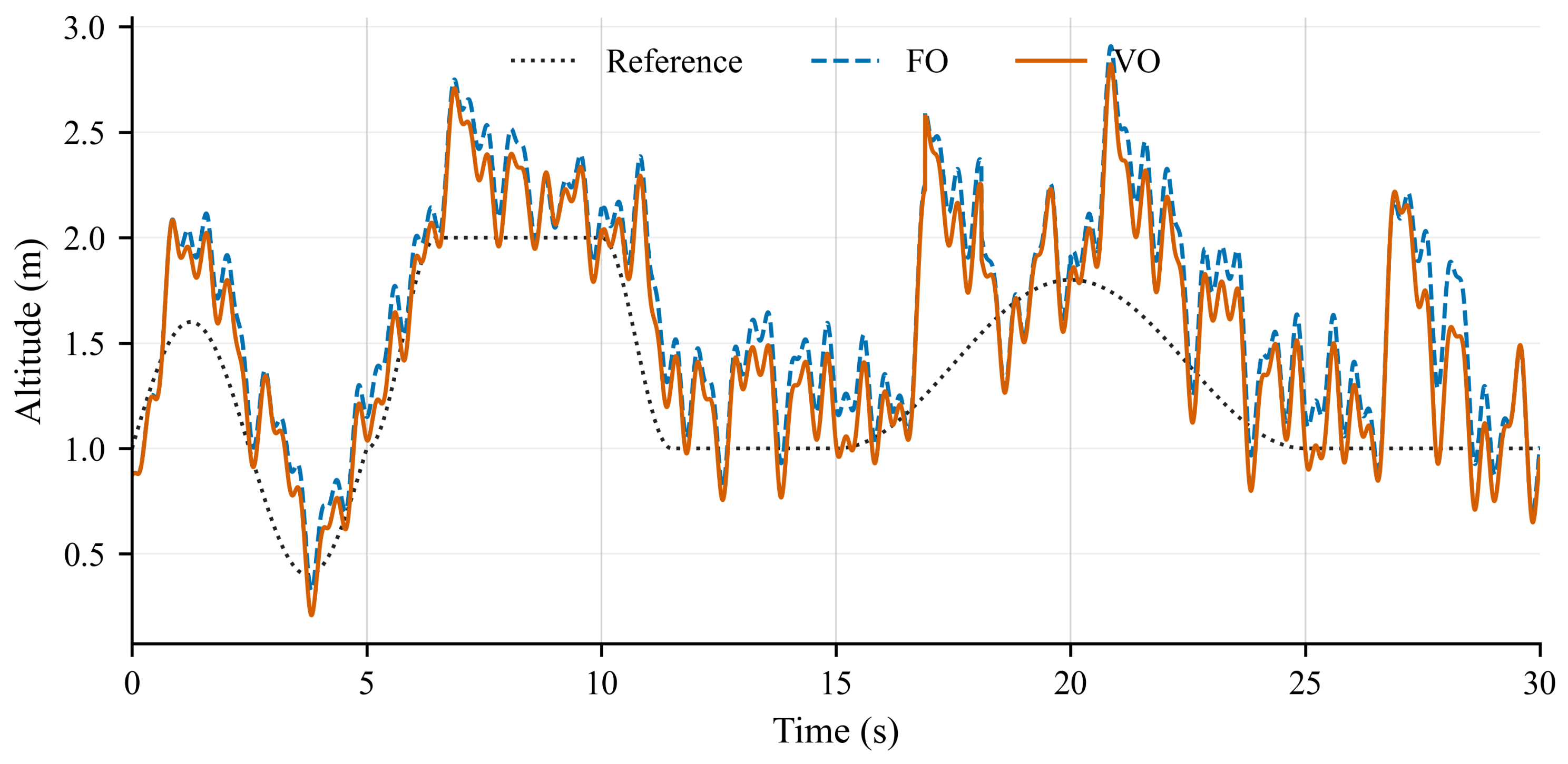
A representative response under the strong-disturbance condition is shown in Figure 7. This trajectory-level comparison complements the aggregate statistics in Table 9 by illustrating the deviation tendency for one archived paired trace.

Figure 7. Representative altitude responses of FO and VO under the strong-disturbance condition ${\kappa }_w=1$ for seed 18.

All controllers degrade under the strong-disturbance condition. Because J is strongly affected by its maximum-error penalty in tail samples, the 62.95% mean reduction in J is not interpreted alone as a direct tracking-error improvement. For the other reported measures, ITAE decreases by 20.41%, $M_p$ by 11.73%, the positive-limit near-saturation ratio by 22.38%, and RMS applied input by 3.48%; the in-band ratio increases by 103.10%. These figures describe the two tested disturbance intensities and do not establish general robustness.

Unlike the baseline condition, the difference between VO and VOITAE with strong disturbance is more visible in the mean of the penalty-sensitive composite index than in ITAE or the input measures. The historical ITAE-trained comparator has the lower mean J in this condition. This difference is not evidence that one training objective is preferable: the controllers do not share the same fixed-order template, neither was retrained for the stronger condition, and no objective-weight sensitivity or restart campaign was performed.

5. Conclusions

This paper compared fixed-order and variable-order fuzzy fractional PID control in a reduced numerical benchmark for quadrotor altitude tracking. The benchmark included first-order motor–propeller dynamics and equivalent net-thrust clipping. The two main controllers shared the fuzzy structure, gain channels, fractional-operator implementation, reference trajectory, disturbance and noise realizations, and evaluation protocol. The variable-order stage optimized four order-scheduling parameters after the fixed-order controller had been obtained.

Under the baseline condition, the paired means and confidence intervals favor VO for the composite index, ITAE, steady-state error, in-band retention, positive-limit near-saturation ratio, and RMS applied input. Overshoot and robust settling time do not show statistically supported improvements, and VO is not better for every seed. The result is therefore a moderate distribution-level difference in the stated metrics, not universal dominance or full-flight evidence.

The baseline counterfactual results are more consistent with the retained online order pattern than with replacement of FO by another constant order pair, but they do not provide an additive causal decomposition. The two pre-specified input indicators—RMS applied input and positive-upper-limit exposure—do not increase for VO, but they do not measure total two-sided clipping. The strong-disturbance test provides a no-retraining comparison at a second intensity; it is not a counterfactual mechanism test, a retuned optimum, a different-spectrum test, or a measurement-noise sensitivity study.

The limitations are also clear. The study uses an illustrative reduced near-hover altitude benchmark and simulation-based validation. Full six-degree-of-freedom coupling, rotor allocation constraints, aerodynamic effects, identified propulsion dynamics, real-time embedded implementation, and hardware or semi-hardware experiments are not included. The archived ITAE-trained comparator uses an earlier fixed-order template and lacks its optimizer log, so it cannot support an objective-only ablation claim. Training-set sensitivity, PSO-restart sensitivity, objective-weight sensitivity, measurement-noise-amplitude sensitivity, alternate disturbance spectral content, alternate order-library resolutions, and population-level clipping/guard-activation rates were not evaluated. For these reasons, the conclusions should not be read as full-vehicle, hardware-validation, objective-function, or general-robustness evidence. Future work should test the same comparison protocol with coupled dynamics and identified or experimental actuator models.

Appendix A.1. Final Input Membership Functions and Gain Singletons

Table A1 reports the final triangular membership-function parameters. A triple $(a,b,c)$ denotes $\mathrm{trimf}(x;[a,b,c\left]\right)$. Values outside the normalized input range $[-1,1]$ define the shoulders of the triangles. The table is rounded to six decimal places; the Supplementary FIS files retain full precision.

Table A1. Final triangular membership-function parameters.

Input	Label	a	b	c
$\tilde{e}$	NB	$-2.000000$	$-0.500000$	$1.000000$
$\tilde{e}$	NM	$-1.130192$	$-0.065096$	$1.000000$
$\tilde{e}$	NS	$-1.000000$	$-0.255433$	$0.489133$
$\tilde{e}$	ZO	$-1.692720$	$-0.346360$	$1.000000$
$\tilde{e}$	PS	$-2.000000$	$-0.500000$	$1.000000$
$\tilde{e}$	PM	$-0.327938$	$0.273741$	$0.875420$
$\tilde{e}$	PB	$-1.062471$	$-0.031235$	$1.000000$
$\widetilde{ec}$	NB	$-2.000000$	$-0.500000$	$1.000000$
$\widetilde{ec}$	NM	$-1.000000$	$-0.136009$	$0.727983$
$\widetilde{ec}$	NS	$-2.000000$	$-0.500000$	$1.000000$
$\widetilde{ec}$	ZO	$-0.134626$	$-0.034626$	$0.065374$
$\widetilde{ec}$	PS	$-0.055969$	$0.044031$	$0.144031$
$\widetilde{ec}$	PM	$-0.054972$	$0.258079$	$0.571130$
$\widetilde{ec}$	PB	$-1.021172$	$-0.010586$	$1.000000$

Table A1. Final triangular membership-function parameters.

Input	Label	a	b	c
$\tilde{e}$	NB	$-2.000000$	$-0.500000$	$1.000000$
$\tilde{e}$	NM	$-1.130192$	$-0.065096$	$1.000000$
$\tilde{e}$	NS	$-1.000000$	$-0.255433$	$0.489133$
$\tilde{e}$	ZO	$-1.692720$	$-0.346360$	$1.000000$
$\tilde{e}$	PS	$-2.000000$	$-0.500000$	$1.000000$
$\tilde{e}$	PM	$-0.327938$	$0.273741$	$0.875420$
$\tilde{e}$	PB	$-1.062471$	$-0.031235$	$1.000000$
$\widetilde{ec}$	NB	$-2.000000$	$-0.500000$	$1.000000$
$\widetilde{ec}$	NM	$-1.000000$	$-0.136009$	$0.727983$
$\widetilde{ec}$	NS	$-2.000000$	$-0.500000$	$1.000000$
$\widetilde{ec}$	ZO	$-0.134626$	$-0.034626$	$0.065374$
$\widetilde{ec}$	PS	$-0.055969$	$0.044031$	$0.144031$
$\widetilde{ec}$	PM	$-0.054972$	$0.258079$	$0.571130$
$\widetilde{ec}$	PB	$-1.021172$	$-0.010586$	$1.000000$

The seven singleton levels used by the three gain outputs are

$$\begin{array}{cc}\hfill {\mathcal{K}}_p=& \{6.104908,10.683590,15.262271,19.840952,24.419633,28.998315,30.000000\},\hfill \\ \hfill {\mathcal{K}}_i=& \{0,0.011581,0.028952,0.057904,0.144759,0.347422,0.579037\},\hfill \\ \hfill {\mathcal{K}}_d=& \{0,1.213376,2.426753,4.550161,7.583602,12.133763,15.000000\}.\hfill \end{array}$$

(A1)

The rule table below stores indices into these three sets. Sugeno weighted averaging is applied directly to the indexed singleton values. The same membership functions, gain singletons, and gain-rule indices are used by FO, VO, VOITAE, $V{O}_{\mathrm{frozen}}$, and $V{O}_{\mathrm{noShift}}$.

Appendix A.2. Shared Gain-Rule Consequent Index Template for the Gain Channels

Table A2 gives the shared rule consequent index template for the three gain channels $K_p,K_i,K_d$. Each triplet $(p,i,d)$ denotes the rule output indices of $K_p,K_i,K_d$, rather than the actual gain values; the corresponding singleton values are listed in Equation (A1).

Table A2. Shared gain-rule consequent index template $(K_p,K_i,K_d)$.

$\mathit{e}\setminus \mathit{ec}$	NB	NM	NS	ZO	PS	PM	PB
NB	(7, 2, 7)	(7, 2, 5)	(7, 2, 4)	(7, 2, 2)	(7, 2, 4)	(7, 2, 5)	(7, 2, 7)
NM	(5, 3, 7)	(5, 3, 5)	(5, 3, 4)	(5, 3, 2)	(5, 3, 4)	(5, 3, 5)	(5, 3, 7)
NS	(4, 5, 7)	(4, 5, 5)	(4, 5, 4)	(4, 5, 2)	(4, 5, 4)	(4, 5, 5)	(4, 5, 7)
ZO	(2, 6, 7)	(2, 6, 5)	(2, 6, 4)	(2, 6, 2)	(2, 6, 4)	(2, 6, 5)	(2, 6, 7)
PS	(4, 5, 7)	(4, 5, 5)	(4, 5, 4)	(4, 5, 2)	(4, 5, 4)	(4, 5, 5)	(4, 5, 7)
PM	(5, 3, 7)	(5, 3, 5)	(5, 3, 4)	(5, 3, 2)	(5, 3, 4)	(5, 3, 5)	(5, 3, 7)
PB	(7, 2, 7)	(7, 2, 5)	(7, 2, 4)	(7, 2, 2)	(7, 2, 4)	(7, 2, 5)	(7, 2, 7)

Table A2. Shared gain-rule consequent index template $(K_p,K_i,K_d)$.

$\mathit{e}\setminus \mathit{ec}$	NB	NM	NS	ZO	PS	PM	PB
NB	(7, 2, 7)	(7, 2, 5)	(7, 2, 4)	(7, 2, 2)	(7, 2, 4)	(7, 2, 5)	(7, 2, 7)
NM	(5, 3, 7)	(5, 3, 5)	(5, 3, 4)	(5, 3, 2)	(5, 3, 4)	(5, 3, 5)	(5, 3, 7)
NS	(4, 5, 7)	(4, 5, 5)	(4, 5, 4)	(4, 5, 2)	(4, 5, 4)	(4, 5, 5)	(4, 5, 7)
ZO	(2, 6, 7)	(2, 6, 5)	(2, 6, 4)	(2, 6, 2)	(2, 6, 4)	(2, 6, 5)	(2, 6, 7)
PS	(4, 5, 7)	(4, 5, 5)	(4, 5, 4)	(4, 5, 2)	(4, 5, 4)	(4, 5, 5)	(4, 5, 7)
PM	(5, 3, 7)	(5, 3, 5)	(5, 3, 4)	(5, 3, 2)	(5, 3, 4)	(5, 3, 5)	(5, 3, 7)
PB	(7, 2, 7)	(7, 2, 5)	(7, 2, 4)	(7, 2, 2)	(7, 2, 4)	(7, 2, 5)	(7, 2, 7)

Appendix A.3. Variable-Order Scheduling Templates in the VO Stage

Table A3 and Table A4 give the $\Delta \alpha$ and $\Delta \beta$ template matrices used in the VO stage. The unit is one 0.1-order level. The requested orders are further obtained through scaling, shifting, clipping, selector safeguards, and adjacent-module output interpolation.

Table A3. $\Delta \alpha$ template.

$\mathit{e}\setminus \mathit{ec}$	NB	NM	NS	ZO	PS	PM	PB
NB	3	3	3	3	3	2	2
NM	2	2	2	2	2	1	1
NS	0	1	1	1	1	0	0
ZO	−1	0	0	0	0	0	−1
PS	0	1	1	1	1	0	0
PM	2	2	2	2	2	1	1
PB	3	3	3	3	3	2	2

Table A3. $\Delta \alpha$ template.

$\mathit{e}\setminus \mathit{ec}$	NB	NM	NS	ZO	PS	PM	PB
NB	3	3	3	3	3	2	2
NM	2	2	2	2	2	1	1
NS	0	1	1	1	1	0	0
ZO	−1	0	0	0	0	0	−1
PS	0	1	1	1	1	0	0
PM	2	2	2	2	2	1	1
PB	3	3	3	3	3	2	2

Table A4. $\Delta \beta$ template.

$\mathit{e}\setminus \mathit{ec}$	NB	NM	NS	ZO	PS	PM	PB
NB	0	1	2	2	2	1	0
NM	−1	0	1	1	1	0	−1
NS	−2	−1	0	0	0	−1	−2
ZO	−3	−2	−1	−1	−1	−2	−3
PS	−2	−1	0	0	0	−1	−2
PM	−1	0	1	1	1	0	−1
PB	0	1	2	2	2	1	0

Table A4. $\Delta \beta$ template.

$\mathit{e}\setminus \mathit{ec}$	NB	NM	NS	ZO	PS	PM	PB
NB	0	1	2	2	2	1	0
NM	−1	0	1	1	1	0	−1
NS	−2	−1	0	0	0	−1	−2
ZO	−3	−2	−1	−1	−1	−2	−3
PS	−2	−1	0	0	0	−1	−2
PM	−1	0	1	1	1	0	−1
PB	0	1	2	2	2	1	0

Appendix A.4. PSO Parameter Settings

Table A5. PSO parameter settings.

Parameter	Setting
Swarm size	40
Maximum iterations	200
Stall iteration limit	60
Inertia weight	Linearly decreasing, ${\omega }_{\max }=0.9$,
	${\omega }_{\min }=0.4$
Learning factors	$c_1=c_2=1.5$
Velocity limit	$\pm 0.2$ in each search coordinate
Boundary handling	Boundary reflection
Mutation probability	0.10
Mutation scale	5% of the parameter span
FO-stage dimension	33
VO-stage dimension	4
Archived ITAE-VO script dimension	4
Training seeds	$\{1201,1202,1203,1204,1205\}$
FO-stage optimizer seed	20251116
VO-stage optimizer seed	20251118
Archived ITAE-VO script seed	20260127

Table A5. PSO parameter settings.

Parameter	Setting
Swarm size	40
Maximum iterations	200
Stall iteration limit	60
Inertia weight	Linearly decreasing, ${\omega }_{\max }=0.9$,
	${\omega }_{\min }=0.4$
Learning factors	$c_1=c_2=1.5$
Velocity limit	$\pm 0.2$ in each search coordinate
Boundary handling	Boundary reflection
Mutation probability	0.10
Mutation scale	5% of the parameter span
FO-stage dimension	33
VO-stage dimension	4
Archived ITAE-VO script dimension	4
Training seeds	$\{1201,1202,1203,1204,1205\}$
FO-stage optimizer seed	20251116
VO-stage optimizer seed	20251118
Archived ITAE-VO script seed	20260127

References

- Podlubny, I. Fractional-order systems and PIλDμ-controllers. IEEE Trans. Autom. Control 1999, 44, 208–214. [Google Scholar] [CrossRef] [Scilit]
- Monje, C.A.; Chen, Y.; Vinagre, B.M.; Xue, D.; Feliu-Batlle, V. Fractional-Order Systems and Controls: Fundamentals and Applications; Springer: London, UK, 2010. [Google Scholar] [CrossRef] [Scilit]
- Shah, P.; Agashe, S. Review of fractional PID controller. Mechatronics 2016, 38, 29–41. [Google Scholar] [CrossRef] [Scilit]
- Bashishtha, T.K.; Singh, V.P.; Yadav, U.K.; Sahu, U.K. Fractional-order PID controllers and applications: A comprehensive survey. Annu. Rev. Control 2025, 60, 101013. [Google Scholar] [CrossRef] [Scilit]
- Takagi, T.; Sugeno, M. Fuzzy identification of systems and its applications to modeling and control. IEEE Trans. Syst. Man Cybern. 1985, 15, 116–132. [Google Scholar] [CrossRef] [Scilit]
- Das, S.; Pan, I.; Das, S.; Gupta, A. A novel fractional order fuzzy PID controller and its optimal time domain tuning based on integral performance indices. Eng. Appl. Artif. Intell. 2012, 25, 430–442. [Google Scholar] [CrossRef] [Scilit]
- Kennedy, J.; Eberhart, R. Particle swarm optimization. In Proceedings of the IEEE International Conference on Neural Networks, Perth, Australia, 27 November–1 December 1995; Volume 4, pp. 1942–1948. [Google Scholar] [CrossRef] [Scilit]
- Clerc, M.; Kennedy, J. The particle swarm—Explosion, stability, and convergence in a multidimensional complex space. IEEE Trans. Evol. Comput. 2002, 6, 58–73. [Google Scholar] [CrossRef] [Scilit]
- Coimbra, C.F.M. Mechanics with variable-order differential operators. Ann. Phys. 2003, 12, 692–703. [Google Scholar] [CrossRef] [Scilit]
- Sun, H.G.; Chen, W.; Chen, Y.Q. Variable-order fractional differential operators in anomalous diffusion modeling. Phys. A Stat. Mech. Its Appl. 2009, 388, 4586–4592. [Google Scholar] [CrossRef] [Scilit]
- Samko, S.G. Fractional integration and differentiation of variable order: An overview. Nonlinear Dyn. 2013, 71, 653–662. [Google Scholar] [CrossRef] [Scilit]
- Valerio, D.; Sá da Costa, J. Variable order fractional controllers. Asian J. Control 2013, 15, 648–657. [Google Scholar] [CrossRef] [Scilit]
- Ostalczyk, P. Variable-, fractional-order discrete PID controllers. In Proceedings of the 2012 17th International Conference on Methods and Models in Automation and Robotics, Miedzyzdroje, Poland, 27–30 August 2012; pp. 534–539. [Google Scholar] [CrossRef] [Scilit]
- Sierociuk, D.; Macias, M. Comparison of variable fractional order PID controller for different types of variable order derivatives. In Proceedings of the 2013 14th International Carpathian Control Conference, Rytro, Poland, 26–29 May 2013; pp. 334–339. [Google Scholar] [CrossRef] [Scilit]
- Liu, L.; Pan, F.; Xue, D. Variable-order fuzzy fractional PID controller. ISA Trans. 2015, 55, 227–233. [Google Scholar] [CrossRef] [Scilit] [PubMed]
- Xue, D.; Liu, L.; Pan, F. Variable-order fuzzy fractional PID controllers for networked control systems. In Proceedings of the 2015 IEEE 10th Conference on Industrial Electronics and Applications, Auckland, New Zealand, 15–17 June 2015; pp. 1438–1442. [Google Scholar] [CrossRef] [Scilit]
- Ahmadnia, M.; Hajipour, A.; Tavakoli, H. Robust variable-order fractional PID-LP fuzzy controller for automatic voltage regulator systems. Appl. Soft Comput. 2024, 167, 112268. [Google Scholar] [CrossRef] [Scilit]
- Mahony, R.; Kumar, V.; Corke, P. Multirotor aerial vehicles: Modeling, estimation, and control of quadrotor. IEEE Robot. Autom. Mag. 2012, 19, 20–32. [Google Scholar] [CrossRef] [Scilit]
- Lee, T.; Leok, M.; McClamroch, N.H. Geometric tracking control of a quadrotor UAV on SE(3). In Proceedings of the 49th IEEE Conference on Decision and Control, Atlanta, GA, USA, 15–17 December 2010; pp. 5420–5425. [Google Scholar] [CrossRef] [Scilit]
- Sonugür, G. A review of quadrotor UAV: Control and SLAM methodologies ranging from conventional to innovative approaches. Robot. Auton. Syst. 2023, 161, 104342. [Google Scholar] [CrossRef] [Scilit]
- López-Sánchez, I.; Moreno-Valenzuela, J. PID control of quadrotor UAVs: A survey. Annu. Rev. Control 2023, 56, 100900. [Google Scholar] [CrossRef] [Scilit]
- Jeong, H.; Suk, J.; Kim, S. Control of quadrotor UAV using variable disturbance observer-based strategy. Control Eng. Pract. 2024, 150, 105990. [Google Scholar] [CrossRef] [Scilit]
- Saribas, H.; Kahvecioglu, S. PSO and GA tuned conventional and fractional order PID controllers for quadrotor control. Aircr. Eng. Aerosp. Technol. 2021, 93, 1243–1253. [Google Scholar] [CrossRef] [Scilit]
- Shao, K.; Liu, J.; Li, M. Fractional order PID control of quadrotor UAV based on SA-PSO algorithm. In Proceedings of the International Conference on Computer Science and Communication Technology, Beijing, China, 30–31 July 2022; Volume 12506, pp. 73–81. [Google Scholar] [CrossRef] [Scilit]
- Liu, T.; Chen, Y.; Chen, Z.; Wu, H.; Cheng, L. Adaptive fuzzy fractional order PID control for 6-DOF quadrotor. In Proceedings of the 39th Chinese Control Conference, Shenyang, China, 27–29 July 2020; pp. 2158–2163. [Google Scholar] [CrossRef] [Scilit]
- Lavín-Delgado, J.E.; Zamudio Beltrán, Z.; Gómez-Aguilar, J.F.; Pérez-Careta, E. Controlling a quadrotor UAV by means of a fractional nested saturation control. Adv. Space Res. 2023, 71, 3822–3836. [Google Scholar] [CrossRef] [Scilit]
- Xian, W.; Qi, Q.; Liu, W.; Liu, Y.; Li, D.; Wang, Y. Control of quadrotor robot via optimized nonlinear type-2 fuzzy fractional PID with fractional filter: Theory and experiment. Aerosp. Sci. Technol. 2024, 151, 109286. [Google Scholar] [CrossRef] [Scilit]
- Sahin, I.; Ulu, C. Altitude control of a quadcopter using interval type-2 fuzzy controller with dynamic footprint of uncertainty. ISA Trans. 2023, 134, 86–94. [Google Scholar] [CrossRef] [Scilit] [PubMed]
- Boubakir, A.; Souanef, T.; Labiod, S.; Whidborne, J.F. A robust adaptive PID-like controller for quadrotor unmanned aerial vehicle systems. Aerospace 2024, 11, 980. [Google Scholar] [CrossRef] [Scilit]
- Lei, H.; Ren, J. Nonlinear fractional-order PID with fractional-order filter controller for quadrotor robot. Unmanned Syst. 2025. online first. [Google Scholar] [CrossRef] [Scilit]
- Ray, L.R.; Stengel, R.F. A Monte Carlo approach to the analysis of control system robustness. Automatica 1993, 29, 229–236. [Google Scholar] [CrossRef] [Scilit]
- Tepljakov, A.; Petlenkov, E.; Belikov, J. FOMCON: Fractional-order modeling and control toolbox for MATLAB. In Proceedings of the 18th International Conference Mixed Design of Integrated Circuits and Systems (MIXDES), Gliwice, Poland, 16–18 June 2011; pp. 684–689. [Google Scholar]
- Oustaloup, A. La Dérivation Non Entière: Théorie, Synthèse et Applications; Hermes: Paris, France, 1995. [Google Scholar]
- Milanesi, M.; Padula, F.; Visioli, A. Practical implementation of gain scheduling strategies with FOPID controllers: A bumpless LPV approach. Annu. Rev. Control 2025, 60, 101007. [Google Scholar] [CrossRef] [Scilit]
- Caponetto, R.; Fortuna, L.; Graziani, S.; Xibilia, M.G. Genetic algorithms and applications in system engineering: A survey. Trans. Inst. Meas. Control 1993, 15, 143–156. [Google Scholar] [CrossRef] [Scilit]
- Wilcoxon, F. Individual comparisons by ranking methods. Biom. Bull. 1945, 1, 80–83. [Google Scholar] [CrossRef] [Scilit]
Disclaimer/Publisher’s Note: The statements, opinions and data contained in all publications are solely those of the individual author(s) and contributor(s) and not of MDPI and/or the editor(s). MDPI and/or the editor(s) disclaim responsibility for any injury to people or property resulting from any ideas, methods, instructions or products referred to in the content. |
© 2026 by the author. Licensee MDPI, Basel, Switzerland. This article is an open access article distributed under the terms and conditions of the Creative Commons Attribution (CC BY) license.