Regularized Parameter Identification in the Tumor Growth Model

Abstract

This study addresses the inverse problem of parameter identification in mathematical models of tumor growth under limited and noisy experimental data. Three classical growth models—logistic, Richards, and Gompertz—are investigated in the context of structural and practical identifiability. It is demonstrated that, despite structural identifiability, parameter estimation remains highly unstable due to the ill-posed nature of the inverse problem. A comparative analysis of the Levenberg–Marquardt method and a genetic algorithm shows that improvements in optimization strategies alone do not resolve this instability and may lead to overfitting. To overcome this limitation, a Tikhonov regularization framework is introduced for the Gompertz model, ensuring stable and physically interpretable parameter estimates. The regularized formulation provides a balance between data fidelity and parameter stability, resulting in improved agreement with experimental observations. To further validate the identified parameters, a reaction–diffusion partial differential equation model is employed. Numerical simulations demonstrate that regularized parameters lead to significantly different spatial tumor morphologies, including more compact structures with sharper interfaces, highlighting the impact of inverse problem regularization on forward model predictions. The results confirm that the primary limitation in tumor growth modeling lies in the ill-posedness of the inverse problem rather than in the choice of optimization algorithm. The proposed framework provides a robust approach for parameter identification and improves the reliability of predictive tumor growth models.

1. Introduction

Cancer progression is a multiscale biological process driven by complex interactions between tumor cells, surrounding tissues, and the microenvironment. Despite advances in experimental techniques and medical imaging, direct measurement of key biological parameters determining tumor growth remains challenging. As a result, mathematical modeling has become a powerful tool for transforming observed data into quantitative representations of tumor dynamics [1,2,3,4,5], enabling a better understanding of biological processes and the creation of useful clinical predictions for therapy [6].

In the existing literature, mathematical models are often constructed based on data. For example, in [7], the authors developed an ODE model of osteosarcoma progression to study the interaction between immune cells and the tumor microenvironment. In [8], the authors extended the data-driven system of ordinary differential equations to a reaction–diffusion-advection (RDA) system of equations and coupled it with Biot poroelasticity equations to form a biomechanical model. The model predicts the number of cancer cells and cytokines in the tumor microenvironment and simulates tumor growth. In [9], the authors developed a predictive agent-based model for the progression of prostate cancer bone metastases and the response to Rad²²³. To optimize treatment for the same type of cancer, in [10], the authors used inverse problem solving methods and in vivo studies in in silico models to consider and simulate various disease development scenarios with and without treatment. However, the authors argue that parameter identification can be improved in the predictive model without treatment. Therefore, this study suggests that the use of other models and other optimization techniques can improve the parameter identification results.

This study considers three models for tumor growth description: the logistic model [11], the Gompertz model [12], and the Richards model [13]. A more detailed discussion of the application of the logistic model, particularly its modification, was provided in a previous study [10]. The focus on the Gompertz model is due to its widespread use alongside the logistic model, as well as its strong descriptive ability and good agreement with experimental data, providing reliable predictive performance [14]. The Gompertz model has been applied both to describe the biological growth, such as in broiler chickens [15], and tumor growth, including colon cancer [16], breast cancer, and lung cancer [14]. Early studies primarily focused on describing tumor volume.

This study proposes the identification of model parameters based on in vivo data on the number of prostate cancer cells metastasizing to bone, describing the dynamics of tumor growth, obtained from a sample of 19 mice. These data were generated using a bioluminescence monitoring method: human prostate cancer PC3 cells expressing luciferase (which provides a light signal) were injected into the tibia, and tumor growth dynamics were assessed measuring the intensity of luminescence after administration of D-luciferin, which is proportional to the number of tumor cells [9]. This method allows for non-invasive monitoring of tumor growth dynamics and the evaluation of experimental effects. The same experimental dataset was used in a previous study [10]. The present biological parameter estimates are specific to the investigated tumor model and experimental setting. The regularization workflow may be applied to other datasets, but generalization of the estimated parameter values to other tumor types or animal species requires independent validation.

The study results demonstrate that reducing model complexity improves identifiability and solution stability when experimental data are limited. A comparative analysis of the Levenberg–Marquardt method and a genetic algorithm shows that metaheuristic optimization improves local approximation but leads to parameter instability and overfitting in the presence of limited and noisy data. Furthermore, a Tikhonov-regularized formulation of the inverse problem is proposed for the Gompertz tumor growth model, providing stable and accurate parameter estimation. It is shown that the regularized Gompertz model better captures the asymmetric growth dynamics and saturation behavior, resulting in physically interpretable model predictions.

To validate the identified parameters, a Gompertz PDE model was constructed in the form of a reaction–diffusion equation for spatial modeling and a physically based understanding of tumor growth.

Unlike most existing studies on optimization methods, this study demonstrates that the primary limitation in parameter identification arises from the ill-posedness of the inverse problem, not from the choice of optimization method.

The article is structured as follows: Section 2, Methods, examines mathematical models of cancer tumor growth; Section 2.1 formulates the inverse problem; Section 2.2 analyzes structural and practical identifiability and constructs sensitivity functions. Section 3 presents the results of solving the direct and inverse problems for the logistic and Richards models using the Levenberg–Marquardt method, and for the Gompertz model, using a genetic method and Tikhonov regularization. Section 3.4 presents the validation of the identified parameters through numerical modeling of the PDE. Section 4 and Section 5 summarize the research work.

2. Materials and Methods

Let us consider the problem of tumor cell growth for prostate cancer metastases in bone. To address this, three population dynamics models are used: a modified logistic model, the Richards model, and the Gompertz model.

The logistic growth model with apoptosis is described by the following differential equation:

$${\displaystyle \frac{d{C}_L}{dt}}= \alpha C_L\left(1-{\displaystyle \frac{C_L}{C_{max}}}\right)-g{C}_L,$$

(1)

where $C_L\left(t\right)$ denotes the number of tumor cells at time $t$(day), $\alpha$(day⁻¹)—is the cell proliferation rate (mitosis), $C_{max}$ is the carrying capacity of the environment representing the maximum possible size of the cell population, and $g$(day⁻¹) is the cell death rate (apoptosis). Let us denote the parameters of the right-hand side of the equation as the parameter vector $p_L=(\alpha ,C_{max}, g)$.

The modified logistic model produces a symmetric S-shaped growth curve, which limits its applicability for describing tumor growth. In particular, the maximum growth rate is reached approximately at the midpoint of the process. In real biological systems, especially in tumor growth, the dynamics are often asymmetric: rapid growth is observed in the early stages, followed by a gradual slowdown due to resource limitations, hypoxia, and other biophysical factors.

The Richards model generalizes the logistic growth law by introducing an additional shape parameter $\nu$:

$${\displaystyle \frac{d{C}_R}{dt}}= \alpha C_R\left[1-{\left({\displaystyle \frac{C_R}{C_{max}}}\right)}^{\nu }\right],$$

(2)

where the right-hand side parameters are given by $p_R=(\alpha ,C_{max}, \nu )$. The parameters $\alpha$ and $C_{max}$ have the same interpretation as in (1), while the parameter $\nu$ in the Richards model is a shape parameter that determines the nonlinearity if the inhibitory term and the asymmetry of the growth curve. It controls the position of the inflection point and the transition rate from exponential growth to saturation, allowing the logistic model to be generalized and the dynamics to approximate those of the Gompertz model [17,18]. Increased flexibility, however, is accompanied by reduced parameter identifiability.

For a more accurate description of these dynamics, a special case of the Richards model—the Gompertz model—is considered, which has the following form:

$${\displaystyle \frac{d{C}_G}{dt}}= \alpha C_G\ln \left({\displaystyle \frac{C_{max}}{C_G}}\right),$$

(3)

where the parameter set $p_G=(\alpha ,C_{max})$ has the same interpretation as in (1), but without explicitly accounting for apoptosis, since in this model the growth rate of the cell population decreases logarithmically as the number of cells increases [19,20]. This nonlinearity provides the asymmetric growth dynamics observed in experimental data. The Gompertz model is widely used in biomathematics due to its ability to capture the early phase of rapid tumor growth followed by a gradual slowdown of the process [20].

Thus, $C(t;p)$ and $p$ denote one of the three models ${\{C_L, C_R,C}_G\}$ and the corresponding parameter sets ${\{p_L, p_R,p}_G\}$ from (1), (2), and (3), respectively.

The choice of the Gompertz model for more detailed analysis is motivated by the need for a more accurate representation of tumor growth dynamics consistent with experimental data, as demonstrated in Section 3. Although the logistic model is widely used in population dynamics, it produces a symmetric S-shaped growth curve that does not always reflect real tumor development. Experimental observations indicate that tumor growth is typically asymmetric: rapid cell proliferation occurs at early stages, followed by a gradual slowdown due to limitations in nutrients, oxygen, and other biophysical factors. The Gompertz model captures this behavior through a logarithmic deceleration mechanism, allowing for a more accurate representation of tumor dynamics and improved approximation of experimental data.

2.1. Inverse Problem

The inverse problem consists of determining the parameter set p from the available data on the temporal evolution of the number of cancer cells $C(t;p)$ [21]. Thus, the inverse problem is reduced to an optimization problem formulated to minimize the following functional:

$$J\left(p\right)={\displaystyle {\sum }_{k=1}^K}{\left(C\left(t_k;p\right)-C_k\right)}^2,$$

(4)

where the functional $J\left(p\right)$—is the sum of squared residuals between the model values $C\left(t_k;p\right)$ and experimental data $C_k$ at time points $t_k$, and $K$ is the total number of experimental time points. For comparison purposes, the optimization problem was solved using the Levenberg–Marquardt method [22,23] for the Richards and Gompertz models, as in [10], as well as using a genetic algorithm [24].

In the sense of Hadamard, the problem is ill-posed due to instability with respect to data perturbations. To ensure solution stability, Tikhonov regularization is applied, leading to the following formulation:

$$J\left(p\right)={\displaystyle {\sum }_{k=1}^K}{\left(C\left(t_k;p\right)-C_k\right)}^2+\lambda {‖p-p_0‖}^2,$$

(5)

where $\lambda >0$ is the regularization parameter and $p_0$ is the initial guess. The addition of the penalty term is equivalent to replacing the matrix ${F=S}^{\top }S$ with $S^{\top }S+\lambda I$, where $S_{kj}={\displaystyle \frac{\partial C(t_k;p)}{\partial p_j}}$. This ensures stability, uniqueness, and suppression of overfitting, and leads to physically interpretable parameter estimates under limited and noisy data conditions; the classical foundations of the method were established by Andrey Tikhonov [25].

This confirms that instability is an inherent property of the problem and cannot be resolved by optimization alone.

2.2. Identifiability

An important aspect of solving the coefficient inverse problem is the preliminary analysis of identifiability. It is necessary to establish the uniqueness of parameter reconstruction from the observed data [26].

For the modified logistic model (1) of cancer cell growth, the original parameterization $p=\left(\alpha ,g,C_{\mathrm{m}\mathrm{a}\mathrm{x}}\right)$ is not structurally identifiable. Only specific combinations of these parameters are identifiable, namely $p=\left(-{\displaystyle \frac{\alpha }{C_{max}}},a-g\right)$, where $a=-{\displaystyle \frac{\alpha }{C_{max}}}$ and $b=a-g$, while the individual parameters $\alpha$, $g$, and $C_{\mathrm{m}\mathrm{a}\mathrm{x}}$ are structurally non-identifiable [10].

2.2.1. Structural Identifiability Analysis

Let us perform a structural global identifiability analysis for the Gompertz model.

$${\displaystyle \frac{d{C}_G}{dt}}=\alpha C_G\ln \left({\displaystyle \frac{C_{max}}{C_G}}\right).$$

To prove its identifiability, the following definition is used [27].

Definition 1. 

Let the observable quantity be $C\left(p,t\right)\equiv C\left(t;\overline{p}\right)$ , Then the parameter  $p$ is structurally globally identifiable if

$$C\left(t;p\right)=C\left(t;\overline{p}\right);\forall p\in {\Omega }_p;\forall t\in [0,T]⟹ p=\overline{p}$$

Let there exist two parameter sets $p_G=(\alpha ,C_{max})$ and ${\overline{p}}_G=(\overline{\alpha },{\overline{C}}_{max})$, and suppose that the corresponding solutions coincide:

$$C_G\left(t;p_G\right)={\overline{C}}_G\left(t;{\overline{p}}_G\right), \forall t$$

Both functions satisfy (3):

$${\displaystyle \frac{d{C}_G}{dt}}= \alpha C_G\ln \left({\displaystyle \frac{C_{max}}{C_G}}\right),$$

(6)

and

$${\displaystyle \frac{d{\overline{C}}_G}{dt}}=\overline{\alpha }{\overline{C}}_G\ln \left({\displaystyle \frac{{\overline{C}}_{max}}{{\overline{C}}_G}}\right),$$

(7)

Since $C_G\left(t;p\right)={\overline{C}}_G\left(t;{\overline{p}}_G\right)$, then

$${\displaystyle \frac{d{C}_G}{dt}}={\displaystyle \frac{d{\overline{C}}_G}{dt}}.$$

(8)

Substituting (6) and (7) into (8), we obtain:

$$\left(\overline{\alpha }-\alpha \right)\ln C_G=\overline{\alpha }\ln {\overline{C}}_{max}-\alpha \ln C_{max}.$$

(9)

The right-hand side of this equation is constant, whereas the left-hand side depends on time. Therefore, the equality holds for all $t$ only if the coefficients coincide:

$$\overline{\alpha }-\alpha =0,$$

which implies

$$\overline{\alpha }=\alpha .$$

Substituting this into (9), we obtain:

$$0=\alpha (\ln {\overline{C}}_{max}-\ln C_{max}),$$

hence,

$${\overline{C}}_{max}=C_{max}.$$

Thus, if $C_G\left(t;p_G\right)={\overline{C}}_G\left(t;{\overline{p}}_G\right)$, then $\left(\alpha ,C_{max}\right)=(\overline{\alpha },{\overline{C}}_{max})$, and the Gompertz model is structurally globally identifiable.

For the Richards model (2)

$${\displaystyle \frac{d{C}_R}{dt}}=\alpha C_R\left[1−{\left({\displaystyle \frac{C_R}{C_{max}}}\right)}^{\nu }\right], C_R(0)=C_{R0}>0,$$

a structural global identifiability analysis is performed analogically as for the Gompertz model, but with twice differentiating. Thus, $C_R\left(t;p_R\right)={\overline{C}}_R\left(t;{\overline{p}}_R\right)$ implies $\left(\alpha ,C_{max},\nu \right)=(\overline{\alpha },{\overline{C}}_{max},\overline{\nu })$, and therefore the Richards model is structurally globally identifiable for $\nu \ne 0, 1$.

Unlike the Gompertz model, the Richards model identifiability proof requires the additional restriction $\nu \notin \left\{0, 1\right\}$. Since at $\nu =1$ the Richards model degenerates into the logistic model, and as $\nu \to 0$ it converges to the Gompertz model, whose identifiability analysis is shown above.

2.2.2. Practical Identifiability Analysis

In this section, the practical identifiability of parameters in tumor growth models is investigated based on sensitivity analysis and the sensitivity matrix. The Gompertz and Richards models are considered.

The practical identifiability of model parameters is evaluated using the sensitivity matrix, which characterizes the dependence of the model solution on the parameters [28]. Let the observable quantity be defined as $\partial C(t_k;p)$, where $p=\left(p_1,p_2,\dots ,p_m\right)$ denotes the vector of model parameters. Then, the sensitivity matrix is defined as:

$$S_{kj}={\displaystyle \frac{\partial C(t_k;p)}{\partial p_j}}.$$

(10)

Based on the sensitivity matrix, the Fisher information matrix is constructed [29,30]:

$$F=S^{\mathrm{\top }}S.$$

(11)

The sensitivity matrix and the associated Fisher information matrix play a key role in the analysis of practical identifiability. If

$$\mathrm{r}\mathrm{a}\mathrm{n}\mathrm{k}\left(S\right)=m,$$

(12)

that is, the rank of the sensitivity matrix equals the number of parameters, then the parameters are locally identifiable. Otherwise, linear dependence between the columns of the matrix indicates non-identifiability of the parameters. Even in the case of full rank, poor conditioning of the Fisher matrix leads to numerical instability in parameter estimation and high sensitivity to data noise. In the area of the minimum of the residual functional, its Hessian is approximated by the Fisher matrix, which determines the local properties of stability and accuracy of the inverse problem solution.

Thus, the analysis of sensitivity functions presented below is equivalent to studying the structure of the sensitivity matrix and the conditioning of the Fisher information matrix. Low sensitivity of parameters leads to degeneracy or poor conditioning of the matrix $F$, which makes the parameter reconstruction problem ill-posed and increases the necessity of regularization.

A 95% confidence interval is reported for each parameter, obtained from the linearized covariance approximation $Cov(p^{\ast })\approx {\sigma }^2{\left(S^{T}S\right)}^{-1}$, where ${\sigma }^2 = RSS\left(p^{\ast }\right)/(K-m)$ is the residual variance and the critical value is taken from Student’s t-distribution with $K-m$ degrees of freedom, to account for the small sample size ($K = 6$).

2.2.3. Sensitivity-Based Analysis for Tumor Growth Models

Sensitivity functions characterize the dependence of the model solution on its parameters. Low sensitivity leads to instability in parameter estimation. The sensitivity functions [31] are defined as:

$$S_i^j\left(t\right)={\displaystyle \frac{\partial C^j(t;p^j)}{\partial p_i^j}}, i=1,\dots ,m; j=1,\dots ,n.$$

(13)

Here, $C(t;p)$ denotes the model solution, $n$ is the number of parameters, and $m$ is the number of models under consideration.

For the Gompertz model (3), the analytical solution has the form:

$$C_G\left(t\right)=C_{max}{\left({\displaystyle \frac{C_{max}}{C_0}}\right)}^{-e^{-t\alpha }}.$$

(14)

The sensitivity coefficients for model (3) are computed analytically:

$$S_{\alpha }^G\left(t\right)=C_{max}{\left({\displaystyle \frac{C_{max}}{C_0}}\right)}^{-e^{-t\alpha }}·t{e}^{-t\alpha }\ln \left({\displaystyle \frac{C_{max}}{C_0}}\right)$$

(15a)

$$S_{C_{max}}^G\left(t\right)={\left({\displaystyle \frac{C_{max}}{C_0}}\right)}^{-e^{-t\alpha }}-{\left({\displaystyle \frac{C_{max}}{C_0}}\right)}^{-e^{-t\alpha }}{·e}^{-t\alpha }.$$

(15b)

The analysis demonstrates good conditioning of the Gompertz model, which explains its superior performance in solving the inverse problem, provided that observations are available over a sufficiently wide time interval. Under these conditions, the sensitivity matrix has full rank:

$$\mathrm{r}\mathrm{a}\mathrm{n}\mathrm{k}\left(S\right)=2,$$

and the Fisher matrix is non-singular, ensuring stable parameter reconstruction. However, deterioration of conditioning may occur when observations are concentrated near the initial time, where sensitivities are small. In the case $C_0\approx C_{\mathrm{m}\mathrm{a}\mathrm{x}}$, the parameter $\alpha$ becomes weakly identifiable, and over a narrow time interval strong correlation between parameters arises.

For the Richards model (2), the analytical solution is typically implicit; therefore, sensitivities are computed numerically using finite differences:

$$S_i\left(t\right)\approx {\displaystyle \frac{C\left(t;p_i+\delta \right)-C\left(t;p_i-\delta \right)}{2\delta }}, i=1,\dots ,n,$$

(16)

where $\delta$ is a small perturbation used in the finite difference approximation. For analysis, normalized sensitivities are used:

$$S_i^{\ast }\left(t\right)={\displaystyle \frac{p_i}{C(t;p)}}{\displaystyle \frac{\partial C(t;p)}{\partial p_i}}.$$

(17)

As a result, for the parameters of model (2), the following sensitivities are obtained:

$$S_{C_{max}}^{R\ast }\left(t\right)\approx 0, \forall t\in [0,T]$$

(18a)

$$S_v^{R\ast }\left(t\right) \mathrm{is} \mathrm{unstable}$$

(18b)

which indicates that model (2) is practically insensitive to the parameter $C_{max}$, while the shape parameter $v$ exhibits unstable behavior. This implies that reliable estimation of these parameters from the available data is not possible.

From the perspective of the sensitivity matrix, the Richards model (2) has full rank:

$$\mathrm{r}\mathrm{a}\mathrm{n}\mathrm{k}\left(S\right)=3.$$

This is consistent with the result of structural identifiability. However, despite structural identifiability, practical identifiability strongly depends on the informativeness of the data, especially on the presence of observations in the saturation region.

Thus, the conducted analysis shows that the Gompertz model possesses more stable practical identifiability of parameters, whereas the Richards model demonstrates conditioning issues and low sensitivity of certain parameters. The stability of the inverse problem solution is directly related to the structure of the sensitivity matrix and the conditioning of the Fisher matrix.

The obtained results confirm the necessity of applying regularization methods in solving inverse problems of parameter identification in tumor growth models.

3. Results

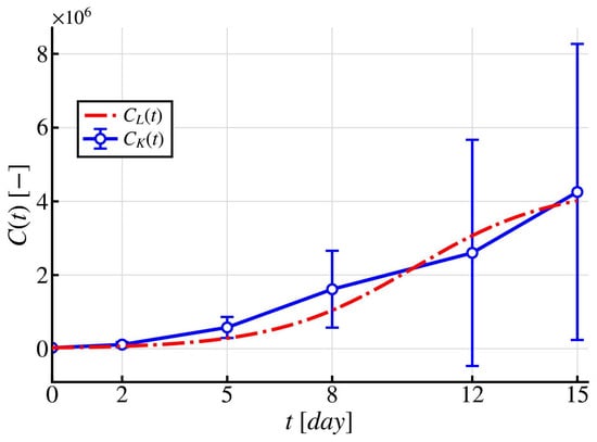
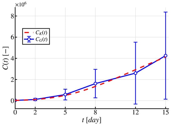
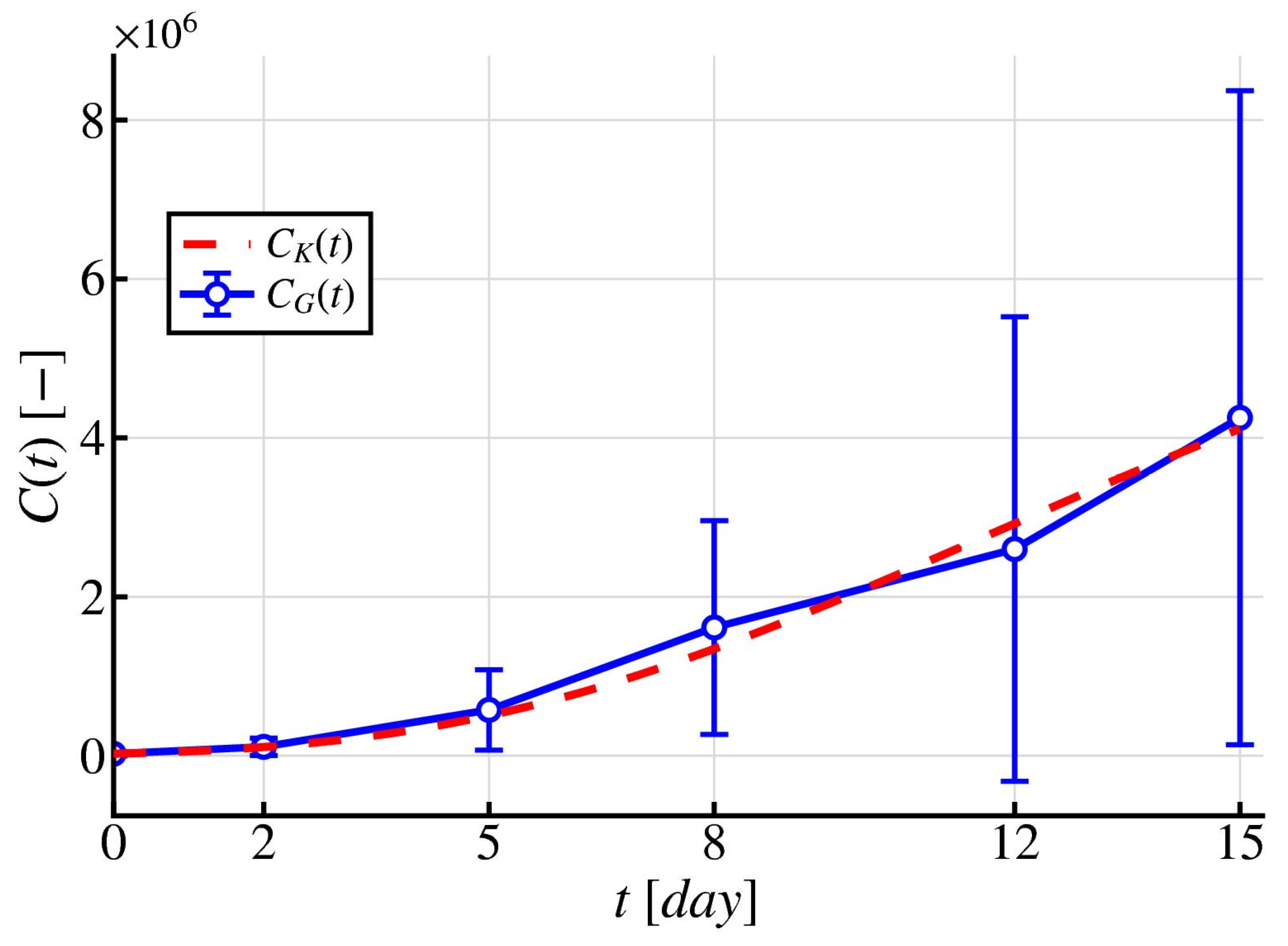
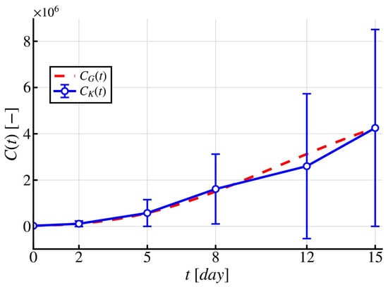
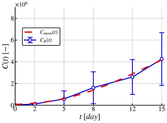
As noted in the Introduction, the parameter estimates reported below pertain specifically to the PC3 prostate-cancer bone-metastasis dataset used in this study; while the identifiability and regularization methodology is general, the numerical results themselves have not been validated on other tumor types or species. The results of the previous study showed that the available set of experimental data is insufficient for the robust identification of the parameters of the generalized growth model. Sensitivity analysis—based on comparing the Taylor-linearized sensitivity region of the model solution against the standard deviation of the experimental measurements, following the approach of [10]—demonstrated that the model sensitivity exceeds the standard deviation of the measurements only at the time points $t=\{12, 15\}$ days, making these as the most informative points for parameter identification. This indicates a high level of uncertainty in parameter reconstruction (Table 1) and, consequently, low reliability of the obtained estimates. In addition, the model predictions exhibit a tendency toward saturation at a level of approximately $4\cdot {10}^6$ [10], corresponding to the stationary state of the model, whereas the experimental observations indicate that the tumor is still in the growth phase (Figure 1).

Table 1. Identified parameters of modified logistic model [10].

Parameter	Value	Units
$\alpha$	1.0001	[day−1]
$C_{max}$	8,414,147	[-]
$g$	0.50005	[day−1]

Figure 1. Predictive modified logistic model describing the dynamics of cancer cells $C_L\left(t\right)$ with the identified parameters $p_L=(\alpha , g, C_{max})$ from [10]—red dashed line, while the blue solid line with circles represents the experimental data $C_k$.

Such a discrepancy between the model predictions and the experimental data indicates parameter identifiability issues within more flexible growth models under limited data availability.

In this regard, the present study employs the Richards growth model and the Gompertz growth model using experimental data (Table 2) obtained from mice with prostate cancer bone metastases reported in [10], based on the mean values of 19 mice with no treatment. Numerical simulations were performed in Python (v3.14.2: df793163d58) on an Apple M5 device with 16 GB RAM.

Table 2. The mean value of tumor cells from the in vivo data [10].

Day	${\mathit{C}}_{\mathit{k}}$ as In Vivo Data	Standard Deviation
0	24,864	23,994
2	112,059	99,399
5	577,111	746,142
8	1,614,381	1,462,355
12	2,601,221	1,602,812
15	4,253,605	2,428,198

3.1. Richards Model

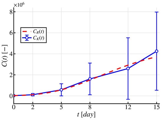
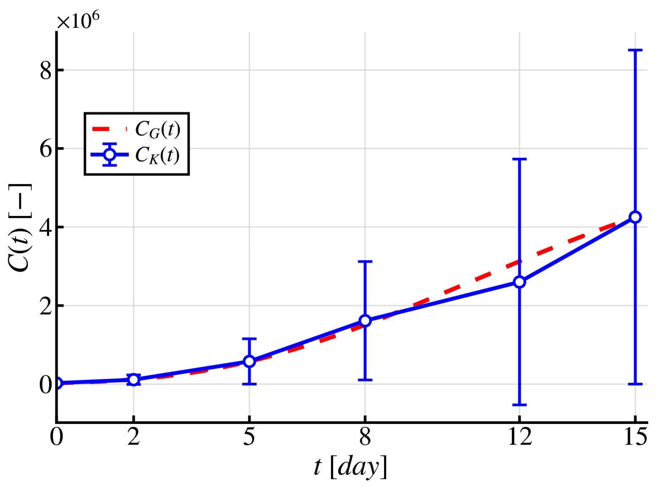
As a result of solving the inverse problem (Figure 2) for the Richards growth model (2) using the Levenberg–Marquardt algorithm optimization method, it was established that this model demonstrates a higher level of agreement with the experimental data compared to the previously considered approach (Figure 1). In particular, within the time interval from day 0 to day 8, a satisfactory degree of convergence between the computed and experimental values is observed. However, with further increase in time up to day 15, a significant discrepancy between the model predictions and the experimental data becomes apparent, indicating the limited accuracy of the model in describing the later stages of the growth process.

Figure 2. Predictive Richards growth model describing the dynamics of cancer cells $C_R\left(t\right)$ with the identified parameters $p_R=(\alpha , C_{max}, v)$—red dashed line, while the blue solid line with circles represents the experimental data $C_k$.

It follows from Table 3 that the parameter $C_{max}=\mathrm{4,864,142}$, which characterizes the carrying capacity of the environment, only slightly exceeds the final number of cancer cells observed on the last day of the experimental measurements ($C_k\left(15\right)=\mathrm{4,253,605}$). This indicates the need for selecting a more adequate model to describe the growth dynamics of prostate cancer bone metastasis cells.

Table 3. Identified parameters of Richards model.

Parameter	Value	Lower CI	Upper CI	Units
$\alpha$	1.999982	−36.87	40.87	[day−1]
$C_{max}$	4,864,142	−4,644,386	14,372,670	[-]
$\upsilon$	0.108905	−2.44	2.66	[-]

Notably, all three $95\%$ confidence intervals include zero and extend into physically inadmissible negative values, which quantitatively confirms the near-total practical non-identifiability of the Richards parameters already indicated by the normalized sensitivity analysis Equation (18a,b).

3.2. Gompertz Model

Preliminary analysis showed that the modified logistic model and the Richards growth model exhibit significant discrepancies with the experimental data, especially at the final point of the time interval. In this regard, the inverse problem was solved to determine the parameter values of the Gompertz growth model (3), also using the Levenberg–Marquardt algorithm optimization method.

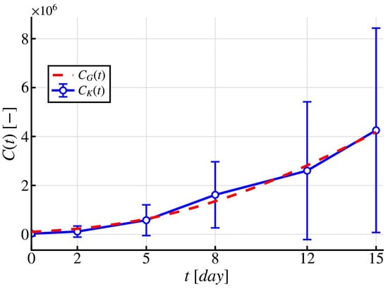
The Gompertz growth model is a more flexible alternative for describing the asymmetric dynamics of tumor cell growth and provides a more accurate approximation of the experimental data (Figure 3). However, deviations are still observed at intermediate stages; for example, on day 8, the absolute error between the experimental data and the model prediction is approximately $2.6\times {10}^5$. Similar discrepancies are also observed on day 12.

Figure 3. Predictive Gompertz growth model describing the dynamics of cancer cells $C_G\left(t\right)$ with the identified parameters $p_G=(\alpha , C_{max})$—red dashed line, while the blue solid line with circles represents the experimental data $C_k$.

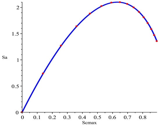
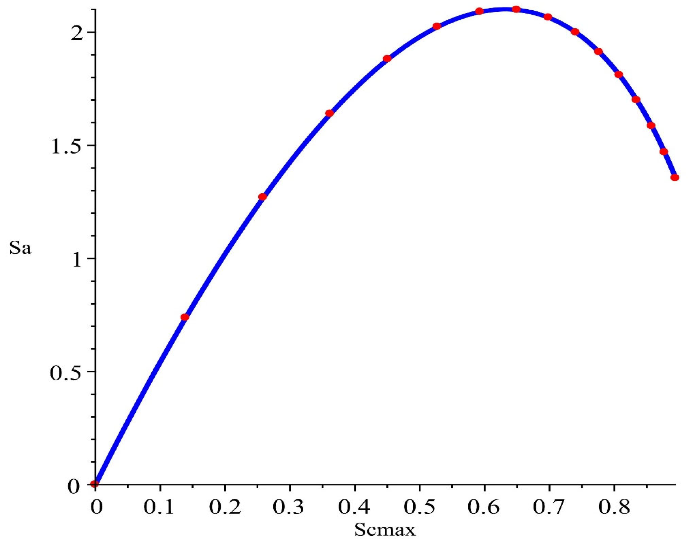
The parametric plot (Figure 4) of the normalized sensitivities demonstrates a smooth and well-defined relationship between the parameters $\alpha$ and $C_{max}$ of the Gompertz growth model. The absence of irregularities indicates stable parameter interaction and a well-conditioned inverse problem. Nevertheless, at the final point (day 15), the Gompertz growth model demonstrates significantly better agreement with the experimental data compared to the logistic and Richards growth models. This indicates its greater capability to accurately reproduce growth saturation and the limiting behavior of the system (Table 4).

Figure 4. Dependence of the sensitivity functions. The blue solid curve represents the continuous sensitivity trajectory, while the red markers indicate the discrete time points at which the sensitivities were evaluated.

Table 4. Identified parameters of Gompertz model.

Parameter	Value	Lower CI	Upper CI	Units
$\alpha$	0.149987	0.0946	0.2053	[day−1]
$C_{max}$	7,512,789	2,590,628	12,434,950	[-]

Thus, the obtained results confirm that the Gompertz growth model is more adequate for describing the considered biological process within the framework of the posed inverse problem. In order to further optimize the model parameters and minimize deviations at intermediate time intervals, a genetic algorithm was applied to this model (Figure 5).

Figure 5. Predictive Gompertz growth model describing the dynamics of cancer cells $C_G\left(t\right)$ with the identified parameters $p_G=(\alpha , C_{max})$ obtained using a genetic algorithm—red dashed line, while the blue solid line with circles represents the experimental data $C_k$.

The results of parameter identification using the genetic algorithm and the subsequent simulation of cancer cell dynamics demonstrated better performance compared to the Levenberg–Marquardt algorithm for the Gompertz growth model, reducing the discrepancies with the experimental data on days 8 and 15, although increasing them relative to the values observed on day 12. The obtained curve reproduces the pattern of changes in the number of cells more accurately and provides a better approximation of the experimental points. This is especially noticeable during the intermediate phases of tumor growth, where the dynamics of the cell population are described more correctly.

From Table 5, it can be observed that the mitosis rate increased by 9%, whereas the carrying capacity, conversely, decreased by approximately 9% as well.

Table 5. Identified parameters of Gompertz model using a genetic algorithm.

Parameter	Value	Lower CI	Upper CI	Units
$\alpha$	0.163551	0.0986	0.2290	[day−1]
$C_{max}$	6,901,224	2,550,394	11,223,621	[-]

Despite these point-estimate differences, the 95% confidence intervals of the two methods overlap substantially and remain within the physically admissible parameter range, indicating that the Levenberg–Marquardt and genetic algorithm solutions are statistically indistinguishable rather than representing genuinely different optima—a further quantitative signature of the ill-posedness discussed in Section 2.1.

To formally compare the two growth models while accounting for their different numbers of parameters, we computed the finite-sample-corrected Akaike Information Criterion (AICc) and the Bayesian Information Criterion (BIC) for each model (Table 6).

Table 6. Formal model comparison (AICc/BIC).

Model	k	AICc	BIC
Richards (Table 3)	3	167.54	154.92
Gompertz, LM (Table 4)	2	153.39	148.97
Gompertz, GA (Table 5)	2	155.68	151.26

Despite using one fewer parameter than the Richards model, both Gompertz parameterizations achieve substantially lower AICc and BIC values, providing formal statistical support for the model selection.

3.3. Tikhonov Regularization

Despite the improvement in approximation achieved using the genetic algorithm, the results demonstrate instability: the reduction in error on days 8 and 15 is accompanied by its increase on day 12. This indicates the sensitivity of the solution to noise and the ill-posedness of the inverse problem of parameter identification for the Gompertz growth model, while the variation in the parameter values suggests overfitting. In this regard, Tikhonov regularization is introduced to ensure solution stability by balancing approximation accuracy and parameter constraints.

The regularized functional has the form (5), where the penalty term $\lambda {‖p-p_0‖}^2$ restricts the deviation of the found parameters from the initial approximation $p_0$, that was set as the values identified by the Levenberg–Marquardt method [10], from Table 1. Specifically, $p_0$ is two-dimensional, comprising only the growth-rate and carrying-capacity estimates from the modified logistic model (Table 1), ${\alpha }_0=1.0001 \left[{\mathrm{d}\mathrm{a}\mathrm{y}}^{-1}\right]$ and ${C_{max}}_0=\mathrm{8,414,147} [-]$; the third logistic-model parameter reported in Table 1 (the apoptosis-related rate: ${\beta }_0=0.50005 \left[{\mathrm{d}\mathrm{a}\mathrm{y}}^{-1}\right]$) has no counterpart in the two-parameter Gompertz model and is therefore excluded from $p_0$. The regularization parameter $\lambda$ was selected from a grid of 40 logarithmically spaced values over the interval $\left(\left[{10}^{-8}, {10}^2\right]\right)$ by minimizing the mean absolute percentage error (MAPE):

$${\lambda }^{\ast }=arg {\min }_{\lambda }MAPE\left(\lambda \right).$$

For each candidate value of $\lambda$, the Gompertz model parameters were re-optimized from scratch. The optimal value was found to be ${\lambda }^{\ast }=0.1512$, which yielded the lowest MAPE and provided a balance between solution stability and approximation accuracy.

To assess the robustness of this choice, we computed the local sensitivity of the regularized estimates to $\lambda$ at the selected value ${\lambda }^{\ast }=0.1512$, using neighboring grid nodes (${\lambda }^{-}\approx 0.0838,{\lambda }^{+}\approx 0.2729$):

$$S_{\alpha }\left(\lambda \right)\approx +0.251,$$

$$S_{C_{max}}\left(\lambda \right)\approx -0.042.$$

This indicates that $\alpha$ is moderately sensitive to $\lambda$ near the operating point, whereas $C_{max}$ is nearly insensitive there, consistent with the $C_{max}\left(\lambda \right)$ curve lying close to a local extremum at ${\lambda }^{\ast }$.

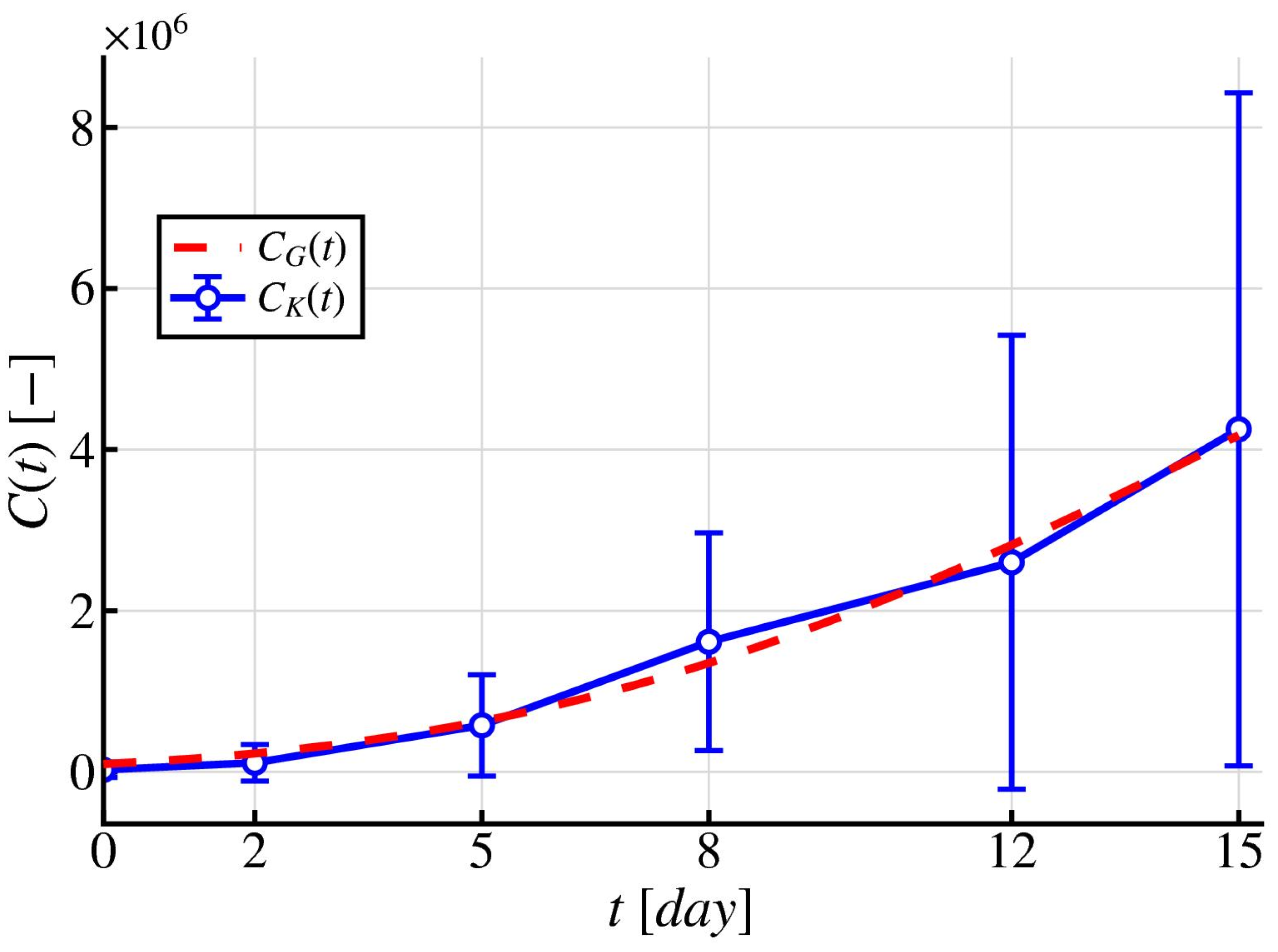
Figure 6, where Tikhonov regularization was applied to the Gompertz growth model, demonstrates more stable and consistent behavior compared to the Levenberg–Marquardt algorithm and the genetic algorithm. In contrast to Figure 5, where overfitting is observed (overestimation of the predicted data on day 12), and Figure 3, which exhibits local deviations, the regularized solution provides uniform agreement with the data across all time intervals. At the same time, the asymmetry of the Gompertz curve is reproduced correctly: the transition from rapid growth to saturation occurs smoothly, without distortions. Saturation is also estimated in a regularized manner—without overestimation and without systematic bias. As a result, a compromise between approximation accuracy and solution stability is achieved, ensuring physically interpretable growth dynamics.

Figure 6. Predictive Gompertz growth model describing the dynamics of cancer cells with the identified parameters $\alpha$ and $C_{max}$ obtained using Tikhonov regularization—red dashed line, while the blue solid line with circles represents the experimental data $C_k$.

Unlike the unregularized Richards and Gompertz estimates (Table 3, Table 4 and Table 5), no confidence interval is reported in Table 7 for the Tikhonov-regularized parameters. The standard linearized-covariance formula used elsewhere in this study assumes an unbiased estimator and is therefore not directly applicable to a biased, regularized solution; deriving a valid bias-corrected interval is left for future work.

Table 7. Identified parameters of Gompertz model using Tikhonov regularization technique.

Parameter	Value	Units
$\alpha$	0.0947	[day−1]
$C_{max}$	13,882,079	[-]
$\lambda$	1.512 × 10−1	[-]

Thus, it is observed that, in contrast to the modified logistic model, parameter reconstruction and subsequent prediction of cancer cell growth dynamics using the Richards growth model and the Gompertz growth model provide more plausible agreement with the experimental data. In the case of the Richards growth model, strong agreement with the experimental data is observed during the early and intermediate periods, accompanied by significant discrepancies at the later stages of the growth process, namely premature saturation of cancer cell growth at a level below $4·{10}^6$ and low values of the carrying capacity $C_{max}$ of the environment, approximately $4.8·{10}^6$.

Better agreement with the experimental data and a more accurate description of the asymmetric growth dynamics are demonstrated by the results of the inverse problem solution for the Gompertz growth model, obtained using both the Levenberg–Marquardt algorithm and the genetic algorithm. This is particularly evident at the later stages of the growth process, with only minor deviations during the intermediate period. In addition, the corresponding estimates of the environmental carrying capacity $C_{max}$ are $7.5·{10}^6$ and $6.9·{10}^6$, respectively.

It should be noted that the parameters identified using regularization technique ($\alpha = 0.0947$ and $C_{\max }=\mathrm{13,882,079}$) differ substantially from the estimates obtained using the Levenberg–Marquardt method and the genetic algorithm. This discrepancy is not a computational artifact but rather reflects a fundamental property of ill-posed inverse problems: when only limited and noisy experimental data are available, multiple parameter sets may yield similarly small values of the misfit functional. Tikhonov regularization selects, from this family of admissible solutions, the one that is most stable with respect to data perturbations and closest to the prior estimate $p_0$.

Although the resulting regularized solution may exhibit a slightly larger residual error than the unregularized estimates, it provides a more stable and physically interpretable set of model parameters. In particular, the estimated carrying capacity $C_{max}=13.8·{10}^6$, suggests that environmental saturation has not yet been reached within the observed time interval, which is consistent with the shape of the experimental growth curve (Table 7).

Table 8 contains a comparative evaluation of the parameter identification methods using the RMSE and MAPE metrics. The Levenberg–Marquardt algorithm yields an RMSE of $1.82·{10}^5$ and a MAPE of $7.85\%$. The genetic algorithm is characterized by the highest RMSE ($2.20·{10}^5$) while providing the lowest MAPE ($5.62\%$). Tikhonov regularization ensures the minimum RMSE value ($1.54·{10}^5$) with a MAPE of $6.73\%$.

Table 8. Error comparison for parameter identification methods.

Method	RMSE	MAPE (%)
Levenberg–Marquardt	$1.82·{10}^5$	$7.85$
Genetic Algorithm	$2.20·{10}^5$	$5.62$
Tikhonov Regularization	$1.54·{10}^5$	$6.73$

To reduce the sensitivity of the solution to the choice of parameter identification method, an aggregated solution is introduced in the form of the pointwise average of the obtained trajectories. Let $C_i\left(t\right),i=1,2,3$, denote the solutions corresponding to the Levenberg–Marquardt algorithm, genetic algorithm, and Tikhonov regularization parameter estimation methods. Then, the averaged trajectory is defined as follows:

$$\overline{C}\left(t\right)={\displaystyle \frac{1}{3}}{\displaystyle \sum _{i=1}^3}{C}_i\left(t\right).$$

This ensemble approximation (Figure 7) provides a regularized description of tumor growth dynamics by reducing the variance associated with the choice of a particular parameter identification method, as well as minimizing the influence of uncertainty in parameter estimation. Note that $C_1\left(t\right),C_2\left(t\right)$, and $C_3\left(t\right)$ are not independent estimates, since all three are fitted to the same dataset with the same model using different parameter estimation procedures, and their errors are therefore correlated through this shared data source. The averaging in the equation should be understood as a heuristic ensemble strategy that reduces sensitivity to the choice of optimization method, rather than a statistically justified estimate of the true trajectory.

Figure 7. Averaged trajectory of cancer cell dynamics $\overline{C}(t)$—red dashed line, while the blue solid line with circles represents the experimental data $C_k$.

Quantitative analysis (Table 8) confirms that regularization improves not only the qualitative characteristics of the solution, but also its overall accuracy. This demonstrates that the instability of parameter identification is inherent to the inverse problem itself and cannot be resolved solely by optimization methods.

3.4. Validation of Identified Parameters in a Reaction–Diffusion Model

Although the obtained results for the ODE models demonstrate good agreement with the experimental data, such models do not account for the spatial heterogeneity of the tumor. In this regard, further validation of the identified parameters is carried out within the framework of a spatially distributed model described by a partial differential equation.

A spatially distributed tumor growth model in the form of a reaction–diffusion equation is considered:

$${\displaystyle \frac{\partial C_G}{\partial t}}=\rho {\nabla }^2{C}_G+ \alpha C_G\ln \left({\displaystyle \frac{C_{max}}{C_G}}\right),$$

(19)

where $C_G=C_G(x,t)$ denotes the spatial distribution of cancer cells, and $\rho >0$ (cm²day⁻¹) is the diffusion coefficient.

Numerical simulation of the PDE model was performed in MATLAB (2025b) using the PDE Toolbox and the finite element method (FEM) [32,33]. Since the present study is aimed at improving the previous results reported in [10], the computations were carried out in a square domain $\left[-1, 1\right]\mathrm{c}\mathrm{m}\times [-1, 1]\mathrm{c}\mathrm{m}$, with the initial tumor geometry represented by an ellipse, as well as with the carrying capacity $C_{max}={10}^6$ and the diffusion coefficient $\rho ={10}^{-4}\mathrm{c}{\mathrm{m}}^2/\mathrm{d}\mathrm{a}{\mathrm{y}}^{-1}$, but using the identified parameters $p_G=(\alpha , C_{max})$ obtained in Section 3.2 and Section 3.3 by the Levenberg–Marquardt algorithm (Table 4), genetic algorithm (Table 5), and Tikhonov regularization (Table 7).

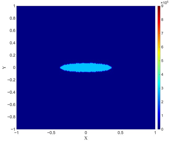
The density (number) distribution of cancer cells at the initial time $t=0$ is presented in Figure 8. The light blue region represents the bone tissue, while the ellipsoidal region at the center represents the cancerous tumor.

Figure 8. Spatial distribution of the tumor cell concentration $C\left(x,y,t\right)$ at $t=0$. The vertical scale on the right denotes the numerical distribution of cancer cells, ranging from 0 to 900,000.

Maximum concentration values (on the order of 280,000) are observed in the central region of the lesion, whereas the concentration rapidly decreases to values close to zero with increasing distance from the center.

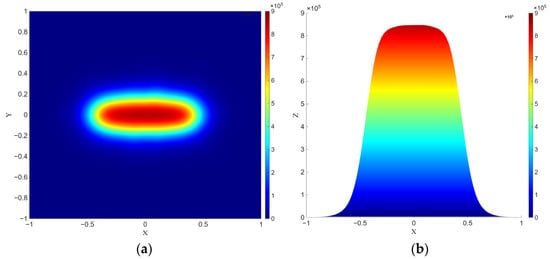
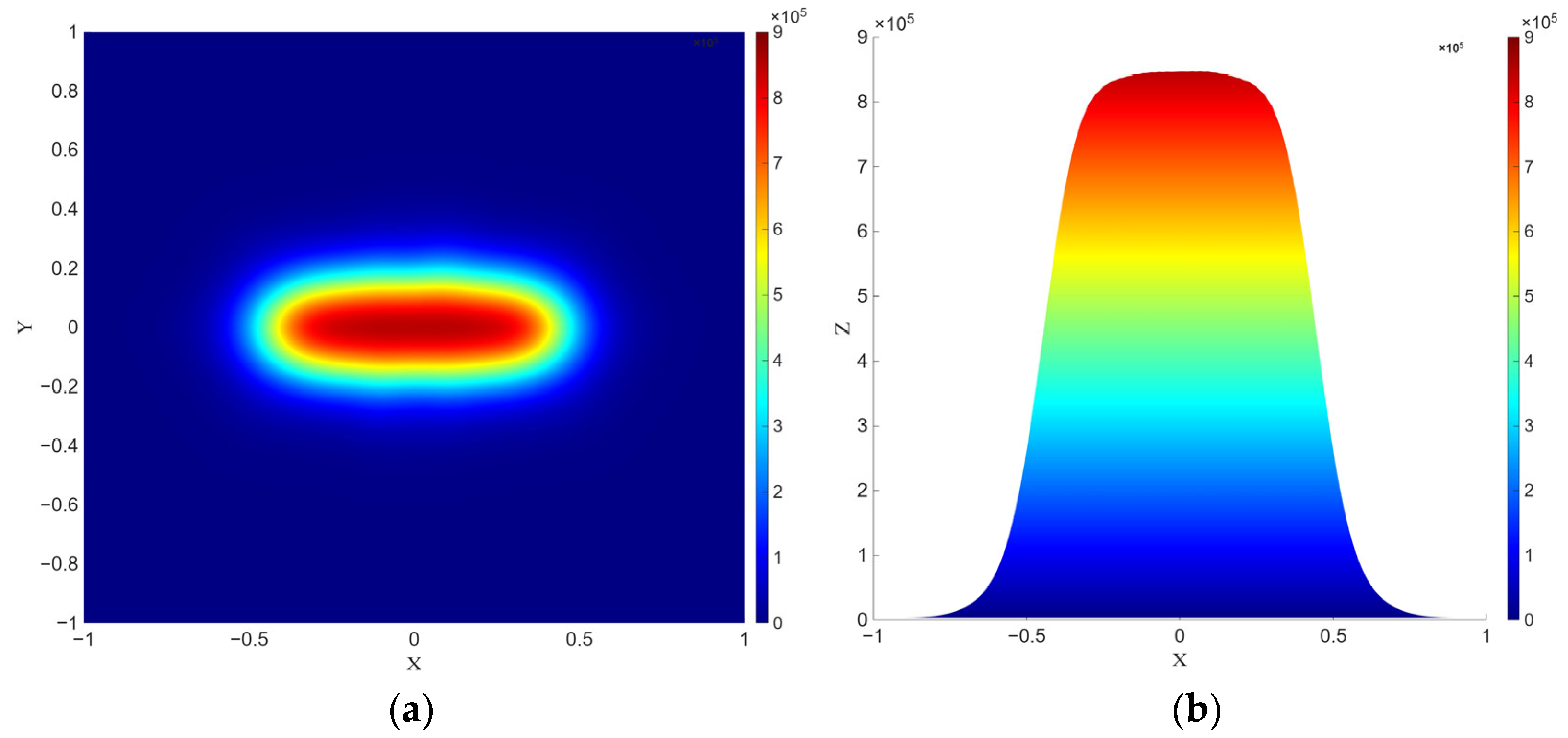
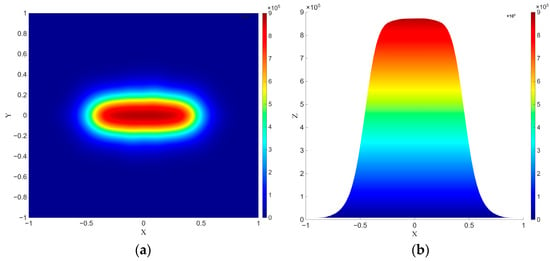
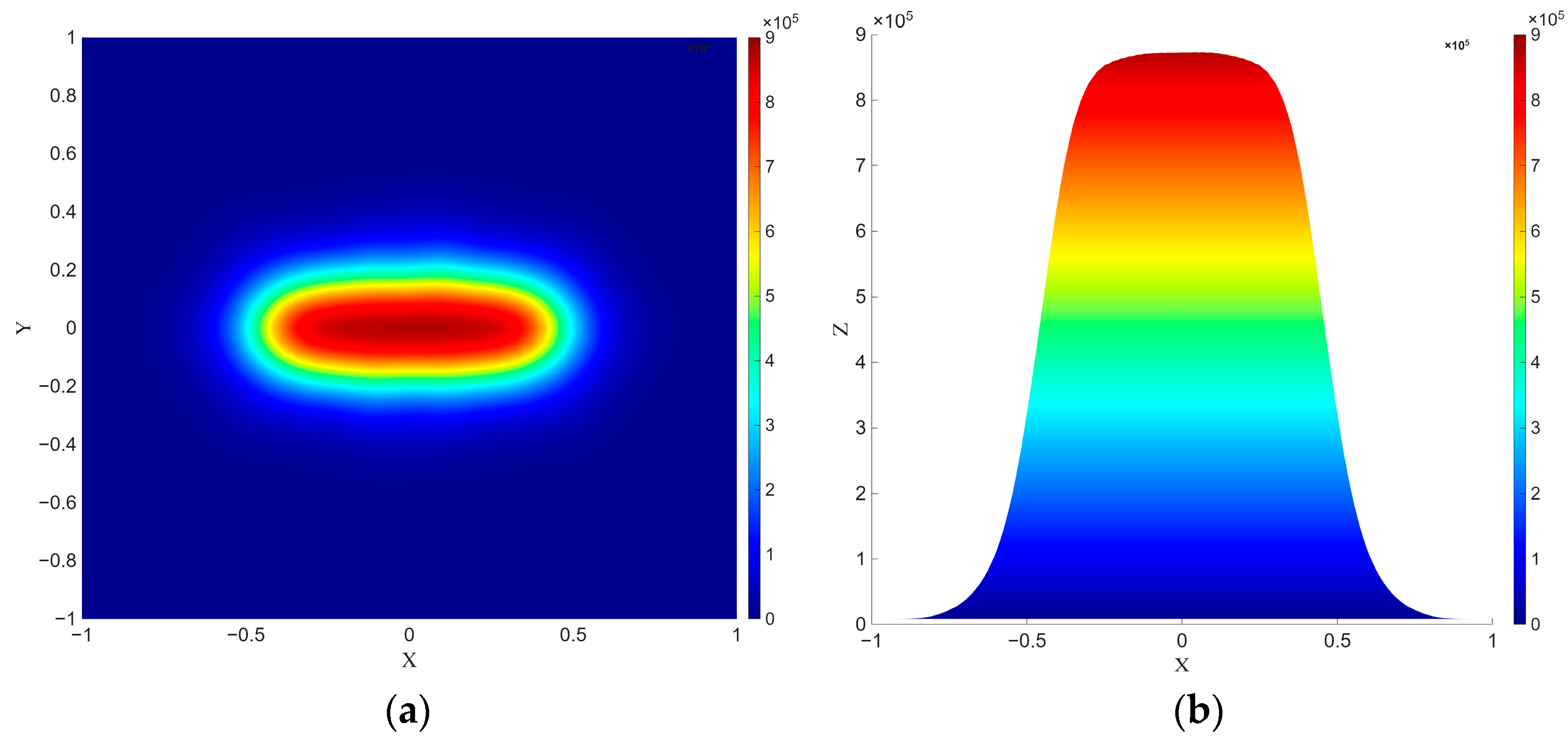
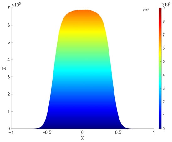
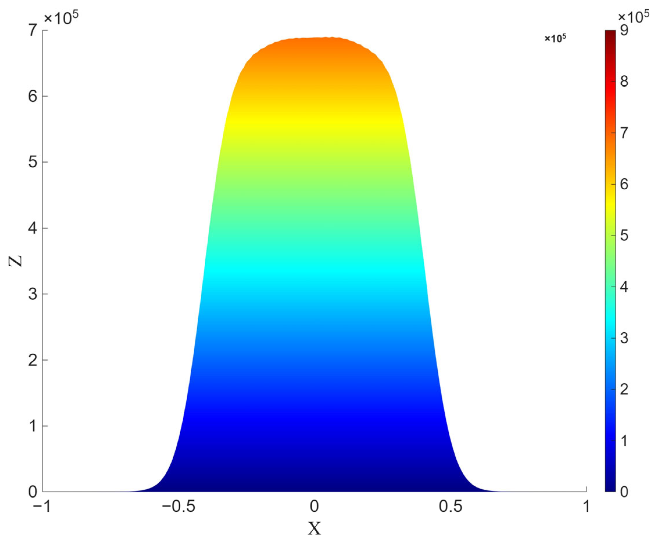
Figure 9, Figure 10, Figure 11, Figure 12 and Figure 13 present the density (number) distribution of cancer cells at the final time $t=15$ using the identified parameters $p_G=(\alpha , C_{max})$ obtained by the Levenberg–Marquardt algorithm (Figure 9), the genetic algorithm (Figure 10), and Tikhonov regularization (Figure 12).

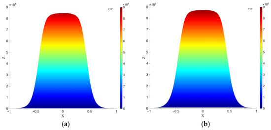
Figure 9. Spatial distribution of the tumor cell concentration $C\left(x,y,t\right)$ at $t=15$ using the identified parameters $p_G=(\alpha , C_{max})$ obtained by the Levenberg–Marquardt algorithm (Table 4): (a) top view ($X-Y$), (b) side view ($X-Z$). The vertical scale on the right denotes the numerical distribution of cancer cells, ranging from 0 to 900,000.

Figure 10. Spatial distribution of the tumor cell concentration $C\left(x,y,t\right)$ at $t=15$ using the identified parameters $p_G=(\alpha , C_{max})$ obtained by genetic algorithm (Table 4): (a) top view ($X-Y$), (b) side view ($X-Z$). The vertical scale on the right denotes the numerical distribution of cancer cells, ranging from 0 to 900,000.

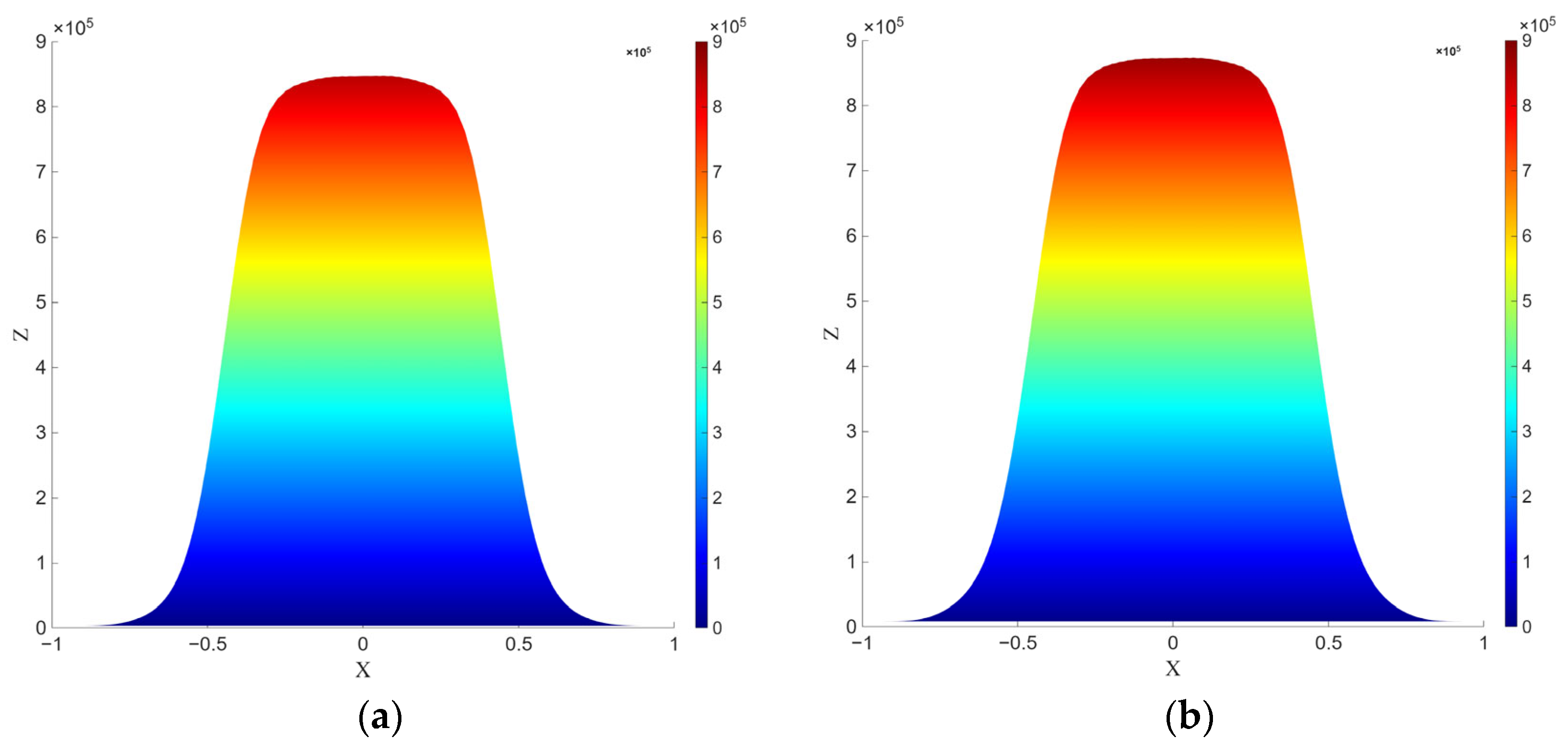
Figure 11. Spatial distribution of the tumor cell concentration $C\left(x,y,t\right)$ at $t=15$ in the $X-Z$ coordinate system: (a) using the identified parameters $p_G=(\alpha , C_{max})$ obtained by the Levenberg–Marquardt algorithm (Table 4), (b) using the identified parameters $p_G=(\alpha , C_{max})$ obtained by the genetic algorithm (Table 5). The vertical scale on the right denotes the numerical distribution of cancer cells, ranging from 0 to 900,000.

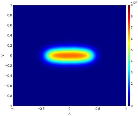
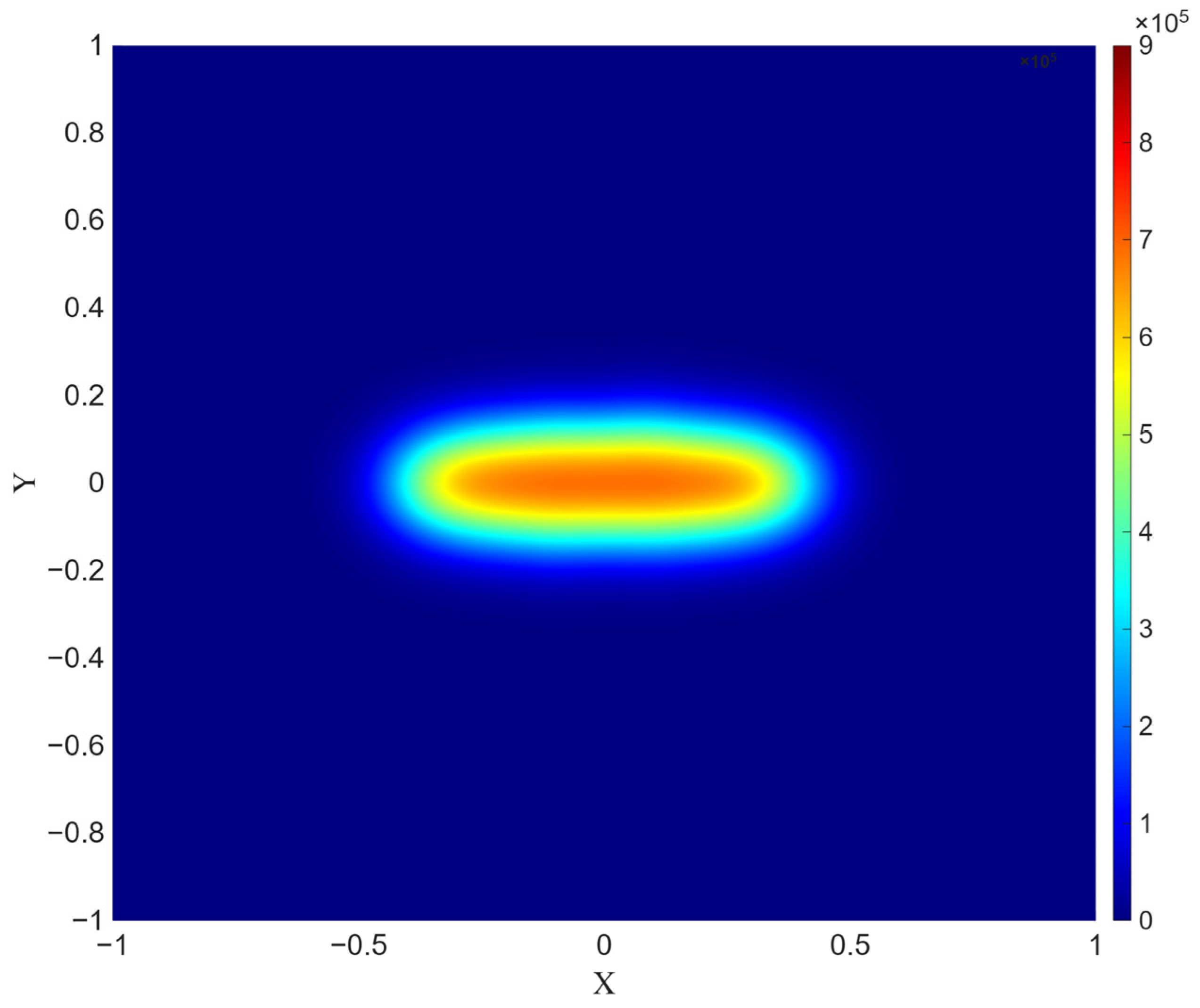
Figure 12. Spatial distribution of the tumor cell concentration $C\left(x,y,t\right)$ at $t=15$ using the identified parameters $p_G=(\alpha , C_{max})$ obtained by Tikhonov regularization (Table 7). The vertical scale on the right denotes the numerical distribution of cancer cells, ranging from 0 to 900,000.

Figure 13. Spatial distribution of the tumor cell concentration $C\left(x,y,t\right)$ at $t=15$ using the identified parameters $p_G=(\alpha , C_{max})$ obtained by Tikhonov regularization in the $X-Z$ coordinate system. The vertical scale on the right denotes the numerical distribution of cancer cells, ranging from 0 to 900,000.

Figure 9 and Figure 10, which present the PDE simulation results obtained using parameters identified by the Levenberg–Marquardt algorithm and the genetic algorithm, respectively, demonstrate a high degree of similarity both in tumor geometry and in the smoothness of the concentration gradient. However, despite the similarity of the transition zone, the simulation using parameters estimated by the genetic algorithm exhibits a wider region (0.928 (Figure 11a) vs. 0.826 (Figure 11b)) and a larger number of cancer cells at the final time point.

In contrast to the Levenberg–Marquardt algorithm and the genetic algorithm, the solution obtained using Tikhonov regularization (Figure 12) demonstrates a different morphology of the concentration distribution. The main feature is the formation of a more compact tumor region with a sharply pronounced boundary, a narrow transition zone, and a smaller tumor radius. The steeper gradients indicate increased solution stability. In addition, the maximum number of cancer cells does not exceed 700,000 (Figure 13).

Therefore, the results of the PDE-based validation (Figure 12 and Figure 13) should not be interpreted as being more accurate in an absolute sense, but rather as regularized. The parameters obtained through regularization are less sensitive to small perturbations in the data, making the corresponding spatial predictions more reproducible and physically interpretable.

To complement the qualitative comparison of Figure 9, Figure 10, Figure 11, Figure 12 and Figure 13, Table 9 reports quantitative metrics of the tumor region at $t = 15$ days for a threshold $\theta = 0.1·C_{max}$: the tumor area $V_{tum}$ (2-D analogue of tumor volume), the boundary length $A_{tum}$ (analogue of surface area), and $G_{mean}/G_{max}$—the mean and maximum gradient magnitude $\left|\mathsf{\nabla }C\right|$ within the tumor region.

Table 9. Quantitative comparison of the identified spatial solutions at $t = 15$.

Model	$${\mathit{V}}_{\mathit{t}\mathit{u}\mathit{m}}$$	$${\mathit{A}}_{\mathit{t}\mathit{u}\mathit{m}}$$	$${\mathit{G}}_{\mathit{m}\mathit{e}\mathit{a}\mathit{n}}/{\mathit{G}}_{\mathit{m}\mathit{a}\mathit{x}}$$
Tikhonov	0.34046	2.3437	2.9484 · 106/4.1823 · 106
LM	0.56104	2.8801	2.6645 · 106/4.0869 · 106
GA	0.65305	3.0735	2.4711 · 106/3.9159 · 106

The Tikhonov-regularized solution yields a smaller tumor area than the LM and GA solutions ($0.34046 \mathrm{v}\mathrm{s}. 0.56104$ and $0.65305$, respectively) and a shorter boundary length, while attaining the highest maximum gradient magnitude ($4.1823·{10}^6 \mathrm{v}\mathrm{s}. 4.0869·{10}^6$ and $3.9159·{10}^6$). This indicates that the regularized solution is more compact without being more diffuse at the tumor boundary.

4. Discussion

The obtained results confirm that the choice of the optimization method is secondary compared to the fundamental issue of the ill-posedness of the inverse problem. Even when using the more flexible genetic algorithm, model overfitting to individual experimental points is observed, manifested in local deviations and parameter instability.

The differences between the parameter estimates obtained through optimization methods and those obtained via regularization do not indicate an error in either approach. Rather, it is a direct consequence of the ill-posed nature of the inverse problem under limited data availability: the solution is inherently unstable, and different methods may converge to distinct regions of the parameter space while yielding similar values of the misfit functional. Tikhonov regularization eliminates instability by restricting the set of admissible solutions. Unlike optimization methods focused solely on minimizing the residual, regularization provides a balance between approximation accuracy and parameter stability, leading to more physically interpretable results.

An important outcome is the correct reproduction of the asymmetric growth dynamics characteristic of tumor processes. The regularized Gompertz growth model adequately describes the early phase of rapid growth and the subsequent slowdown. This ensures the physical interpretability of the parameters.

It should be noted that the dataset used is limited in size and contains significant uncertainty, which complicates reliable parameter identification. In addition, both the ODE and PDE models considered here capture only a restricted subset of tumor biology. The reaction–diffusion formulation (Equation (19)) combines isotropic spatial diffusion with Gompertzian growth kinetics but omits tissue heterogeneity, immune-mediated dynamics, and angiogenesis/nutrient limitation—factors known to shape tumor morphology in vivo. The spatial patterns in Section 3.4 should therefore be read as an illustration of how the identified kinetic parameters propagate into a simplified spatial setting, not as a biologically calibrated prediction, which limits the framework’s direct clinical applicability. Incorporating immune and microenvironmental compartments (in the spirit of [7,8]) is left for future work.

A promising direction is the use of Machine Learning methods, including physics-informed neural networks (PINNs) [34,35], which allow the differential equations of the model to be integrated directly into the training procedure, as well as generative models for expanding the training dataset and reducing data uncertainty. However, such approaches require further investigation in the context of consistency with physically grounded models, including PINNs.

5. Conclusions

The present study compares the results of modeling tumor growth in the bone tissue of laboratory mice for the two considered models with experimental data and with the predictive solution obtained using the modified logistic model. Analysis of the graphs showed that both proposed models reproduce the overall trend of tumor cell growth and demonstrate better agreement with the experimental data. However, the Richards growth model exhibits noticeable deviations from the experimental data at the final time intervals, whereas the Gompertz growth model demonstrates a higher degree of agreement throughout the entire considered time interval.

Thus, the study shows that the Gompertz growth model possesses greater flexibility and provides the best agreement with tumor cell growth dynamics data, especially when combined with the metaheuristic optimization approach based on the genetic algorithm, while Tikhonov regularization ensures stable parameter reconstruction.

Several limitations of this study should be acknowledged. First, the experimental dataset is limited to six unevenly spaced time points from 19 untreated mice, with substantial inter-animal variability, which constrains the practical identifiability of model parameters and restricts the informativeness of the data primarily to the later observation times ($t = 12, 15$ days). Second, the reaction–diffusion PDE validation employed a simplified elliptical tumor geometry and a fixed diffusion coefficient, adapted from [10] rather than identified from the present dataset, and therefore should be interpreted as a qualitative validation of parameter-dependent tumor morphology rather than a quantitatively calibrated spatial prediction. Finally, this study is restricted to three classical growth models (logistic, Richards, Gompertz); extending the identifiability and regularization framework to other model families, incorporating immune and microenvironmental compartments, including data-driven or physics-informed neural network approaches, is left for future work.

References

- Benzekry, S.; Lamont, C.; Beheshti, A.; Tracz, A.; Ebos, J.M.; Hlatky, L.; Hahnfeldt, P. Classical mathematical models for description and prediction of experimental tumor growth. PLoS Comput. Biol. 2014, 10, e1003800. [Google Scholar] [CrossRef] [Scilit] [PubMed]
- Kabanikhin, S.I.; Krivorotko, O.I. Identification of biological models described by systems of nonlinear differential equations. J. Inverse Ill-Posed Probl. 2015, 23, 519–527. [Google Scholar] [CrossRef] [Scilit]
- Barbolosi, D.; Ciccolini, J.; Lacarelle, B.; Barlési, F.; André, N. Computational oncology—Mathematical modelling of drug regimens for precision medicine. Nat. Rev. Clin. Oncol. 2016, 13, 242–254. [Google Scholar] [CrossRef] [Scilit] [PubMed]
- Pompa, M.; Urso, G.; Panunzi, S.; Drexler, D.A.; Gombos, B.; De Gaetano, A. A Mathematical Model of Breast Cancer Growth and Drug Resistance Evolution Under Chemotherapy. Mathematics 2025, 13, 1115. [Google Scholar] [CrossRef] [Scilit]
- Altrock, P.; Liu, L.; Michor, F. The mathematics of cancer: Integrating quantitative models. Nat. Rev. Cancer 2015, 15, 730–745. [Google Scholar] [CrossRef] [Scilit] [PubMed]
- Winsor, C.P. The Gompertz curve as a growth curve. Proc. Nat. Acad. Sci. USA 1932, 18, 1–8. [Google Scholar] [CrossRef] [Scilit] [PubMed]
- Le, T.; Su, S.; Kirshtein, A.; Shahriyari, L. Data-Driven Mathematical Model of Osteosarcoma. Cancers 2021, 13, 2367. [Google Scholar] [CrossRef] [Scilit] [PubMed]
- Hu, Y.; Mohammad Mirzaei, N.; Shahriyari, L. Bio-Mechanical Model of Osteosarcoma Tumor Microenvironment: A Porous Media Approach. Cancers 2022, 14, 6143. [Google Scholar] [CrossRef] [Scilit] [PubMed]
- Casarin, S.; Dondossola, E. An agent-based model of prostate Cancer bone metastasis progression and response to Radium223. BMC Cancer 2020, 20, 605. [Google Scholar] [CrossRef] [Scilit] [PubMed]
- Bektemessov, Z.; Cherfils, L.; Allery, C.; Berger, J.; Serafini, E.; Dondossola, E.; Casarin, S. On a data-driven mathematical model for prostate cancer bone metastasis. AIMS Math. 2024, 9, 34785–34805. [Google Scholar] [CrossRef] [Scilit]
- Verhulst, P.-F. Notice sur la loi que la population suit dans son accroissement. Corresp. Math. ET Phys. 1938, 10, 113–121. [Google Scholar]
- Gompertz, B. On the nature of the function expressive of the law of human mortality, and on a new mode of determining the value of life contingencies. Philos. Trans. R. Soc. Lond. B Biol. Sci. 1825, 182, 513–585. [Google Scholar] [CrossRef] [Scilit]
- Debnath, G.; Vasu, B.; Gorla, R.S.R.; Beg, O.A.; Beg, T.A. Integrating Mathematical Models in Clinical Oncology: Enhancing Therapeutic Strategies. Arch. Pharmacol. Ther. 2025, 7, 1–27. [Google Scholar] [CrossRef] [Scilit]
- Vaghi, C.; Rodallec, A.; Fanciullino, R.; Ciccolini, J.; Mochel, J.P.; Mastri, M.; Poignard, C.; Ebos, J.M.L.; Benzekry, S. Population modeling of tumor growth curves and the reduced Gompertz model improve prediction of the age of experimental tumors. PLoS Comput. Biol. 2020, 16, e1007178. [Google Scholar] [CrossRef] [Scilit] [PubMed]
- Wang, Z.; Zuidhof, M.J. Estimation of Growth Parameters Using a Nonlinear Mixed Gompertz Model. Poult. Sci. J. 2004, 83, 847–852. [Google Scholar] [CrossRef] [Scilit] [PubMed]
- Claret, L.; Girard, P.; Hoff, P.M.; Van Cutsem, E.; Zuideveld, K.P.; Jorga, K.; Fagerberg, J.; Bruno, R. Model-based prediction of phase III overall survival in colorectal cancer on the basis of phase II tumor dynamics. J. Clin. Oncol. 2009, 27, 4103–4108. [Google Scholar] [CrossRef] [Scilit] [PubMed]
- Tjørve, K.M.C.; Tjørve, E. The use of Gompertz models in growth analyses, and new Gompertz-model approach: An addition to the Unified-Richards family. PLoS ONE 2017, 12, e0178691. [Google Scholar] [CrossRef] [Scilit] [PubMed]
- Richards, F.J. A flexible growth function for empirical use. J. Exp. Bot. 1959, 10, 290–300. [Google Scholar] [CrossRef] [Scilit]
- Laird, A.K. Dynamics of tumor growth. Br. J. Cancer 1964, 19, 278–291. [Google Scholar] [CrossRef] [Scilit] [PubMed]
- Norton, L. A Gompertzian model of human breast cancer growth. Cancer Res. 1988, 48, 7067–7071. [Google Scholar] [PubMed]
- Kabanikhin, S.I. Definitions and examples of inverse and ill-posed problems. J. Inverse Ill-Posed Probl. 2008, 16, 317–357. [Google Scholar] [CrossRef] [Scilit]
- Levenberg, K. A Method for the Solution of Certain Non-Linear Problems in Least Squares. Q. Appl. Math. 1944, 2, 164–168. [Google Scholar] [CrossRef] [Scilit]
- Marquardt, D. An Algorithm for Least-Squares Estimation of Nonlinear Parameters. SIAM J. Appl. Math. 1963, 11, 431–441. [Google Scholar] [CrossRef] [Scilit]
- Katoch, S.; Chauhan, S.S.; Kumar, V. A review on genetic algorithm: Past, present, and future. Multimed. Tools Appl. 2021, 80, 8091–8126. [Google Scholar] [CrossRef] [Scilit] [PubMed]
- Tikhonov, A.N. Solution of incorrectly formulated problems and the regularization method. Sov. Math. Dokl. 1963, 4, 1035–1038. [Google Scholar]
- Browning, A.P.; Warne, D.J.; Burrage, K.; Baker, R.E.; Simpson, M.J. Identifiability analysis for stochastic differential equation models in systems biology. J. R. Soc. Interface 2020, 17, 20200652. [Google Scholar] [CrossRef] [Scilit] [PubMed]
- Walter, E.; Lecourtier, Y. Global approaches to identifiability testing for linear and nonlinear state space models. Math. Comput. Simul. 1982, 24, 472–482. [Google Scholar] [CrossRef] [Scilit]
- Kabanikhin, S.; Bektemesov, M.; Krivorotko, O.; Bektemessov, Z. Practical identifiability of mathematical models of biomedical processes. J. Phys. Conf. Ser. 2021, 2092, 012014. [Google Scholar] [CrossRef] [Scilit]
- Trees, V. Detection, Estimation, and Modulation Theory, Part I; Wiley: New York, NY, USA, 1968. [Google Scholar]
- Freiden, B.R. Science from Fisher Information; Cambridge University Press: New York, NY, USA, 2004. [Google Scholar]
- Saltelli, A.; Chan, K.; Scott, M. Sensitivity Analysis; Wiley Series in Probability and Statistics; John Wiley & Son: New York, NY, USA, 2000. [Google Scholar]
- Brenner, S.C.; Scott, L.R. The Mathematical Theory of Finite Element Methods; Springer: Berlin/Heidelberg, Germany, 2007. [Google Scholar] [CrossRef] [Scilit]
- Zienkiewicz, O.C.; Taylor, R.L. The Finite Element Method; Butterworth-Heinemann: Oxford, UK, 2000; Volume 1. [Google Scholar]
- Kisbenedek, L.; Kovács, L.; Drexler, D.A. Physics-Informed Neural Network for Parameter Inference in a Tumor Model. Mathematics 2026, 14, 1102. [Google Scholar] [CrossRef] [Scilit]
- Farea, A.; Yli-Harja, O.; Emmert-Streib, F. Using Physics-Informed Neural Networks for Modeling Biological and Epidemiological Dynamical Systems. Mathematics 2025, 13, 1664. [Google Scholar] [CrossRef] [Scilit]
Disclaimer/Publisher’s Note: The statements, opinions and data contained in all publications are solely those of the individual author(s) and contributor(s) and not of MDPI and/or the editor(s). MDPI and/or the editor(s) disclaim responsibility for any injury to people or property resulting from any ideas, methods, instructions or products referred to in the content. |
© 2026 by the authors. Licensee MDPI, Basel, Switzerland. This article is an open access article distributed under the terms and conditions of the Creative Commons Attribution (CC BY) license.