


Abstract
Portfolio optimization remains a challenging problem due to the dynamic, nonlinear, and uncertain characteristics of financial markets. Traditional portfolio construction approaches, including mean variance optimization and conventional Black–Litterman models, often suffer from inaccurate estimation of expected returns and unstable allocation caused by parameter uncertainty. These limitations become more significant under structural breaks, regime transitions, volatility clustering, and extreme market events. This study proposes a Transformer-GAN enhanced Black–Litterman framework (TG-BL) that integrates temporal representation learning, uncertainty-aware scenario generation, and Bayesian portfolio optimization. The proposed framework consists of three complementary components. First, a Transformer-based encoder is employed to extract long- range temporal dependencies and latent market representations from historical financial sequences. Second, a conditional Generative Adversarial Network (GAN) is introduced to generate diverse future return scenarios conditioned on Transformer- derived market representations, enabling probabilistic modeling of future uncertainty rather than deterministic prediction. Third, the generated return distributions are incorporated into the Black–Litterman framework through dynamically calibrated views and confidence estimation. Unlike conventional approaches that directly replace equilibrium returns with machine-generated predictions, the proposed method preserves the Bayesian structure of Black–Litterman by adjusting the influence of model- generated views according to predictive uncertainty. This mechanism allows AI- based forecasts to complement rather than dominate market equilibrium information. Extensive experiments are conducted using historical financial data under multiple market conditions. The evaluation framework includes portfolio performance comparison, GAN-generated scenario validation, robustness analysis under volatility and liquidity stress, and component- wise ablation experiments. The results demonstrate that the proposed TG-BL framework improves risk-adjusted portfolio performance while maintaining robustness against market uncertainty. The findings indicate that the integration of temporal feature extraction, uncertainty modeling, and Bayesian portfolio allocation provides an effective decision-support framework for quantitative investment management.
MSC:
91G10; 91G15; 91G70
1. Introduction
Portfolio optimization aims to determine asset allocation strategies that achieve an appropriate trade-off between expected return and investment risk [1]. Since the introduction of modern portfolio theory, the mean variance framework proposed by Markowitz has become one of the fundamental approaches in quantitative finance [2,3]. However, traditional mean–variance optimization suffers from estimation errors and unstable portfolio weights [4], which motivates the development of Bayesian portfolio optimization approaches such as the Black–Litterman model.
The Black–Litterman (BL) model was developed to overcome some limitations of traditional portfolio optimization by combining market equilibrium information with investor views through a Bayesian framework [5]. Instead of relying entirely on estimated expected returns, the BL model introduces a mechanism that balances prior market information and additional return expectations according to confidence levels. This property makes the BL framework widely used in institutional portfolio management.
Nevertheless, constructing reliable investor views remains a major challenge. Traditional BL implementations usually depend on subjective assumptions or statistical forecasts, which may fail to capture the complex characteristics of modern financial markets. Financial time series exhibit strong nonlinear relationships, non-stationarity, volatility clustering, regime changes, and heavy- tailed distributions. These characteristics violate many assumptions of conventional statistical models and create difficulties for accurate return estimation.
Recent advances in deep learning have provided new opportunities for financial forecasting and portfolio optimization [6]. Transformer architectures, originally developed for sequential modeling, have demonstrated strong capability in capturing long- range dependencies through self-attention mechanisms [7,8]. Unlike recurrent neural networks that process information sequentially, Transformers can dynamically assign different importance weights to historical observations, allowing them to capture complex temporal relationships in financial data [9].
However, deterministic forecasting models have limitations when applied to financial markets. Future returns are inherently uncertain, and a single predicted value cannot fully describe possible future market scenarios. Therefore, uncertainty modeling is equally important for portfolio construction. Generative models, particularly Generative Adversarial Networks (GANs), provide an alternative approach by learning complex data distributions and generating possible future scenarios [10]. Despite their potential, applying GANs to financial data requires careful consideration [11]. Financial returns are characterized by non-stationarity, heavy tails, and rare extreme events. A generated sequence that only resembles historical observations statistically may not necessarily provide meaningful investment information. Therefore, a financial generative model should not only generate realistic- looking samples but also preserve important market characteristics, including return distributions, dependence structures, and volatility dynamics.
Motivated by these challenges, this study proposes a Transformer-GAN enhanced Black–Litterman framework (TG-BL). The objective is not simply to combine multiple AI models, but to establish a complete information pathway: Historical Market Data → Transformer Representation → Conditional GAN Scenario Generation → Dynamic BL Calibration → Portfolio Optimization.
The proposed framework introduces an explicit interaction mechanism between Transformer and GAN. Transformer representations are used as conditional information to guide GAN scenario generation, allowing generated trajectories to reflect current market conditions. The resulting predictive distribution is then transformed into Black–Litterman views and confidence estimates, enabling uncertainty- aware portfolio allocation.
The main contributions of this study are summarized as follows:
(1) A Transformer-GAN interaction mechanism is proposed.
Different from previous approaches that independently apply prediction and generation models, the proposed framework defines a conditional relationship between Transformer latent representations and GAN-generated financial scenarios.
(2) A dynamic Black–Litterman calibration strategy is developed.
Model-generated views are incorporated through uncertainty-based confidence estimation, preventing machine predictions from excessively dominating market equilibrium information.
(3) A comprehensive evaluation framework is established.
The proposed method is evaluated through portfolio performance analysis, syn-thetic scenario validation, market stress testing, and ablation experiments to identify the contribution of each component.
(4) Practical portfolio constraints are considered.
Transaction costs, turnover limitations, and realistic execution assumptions are incorporated to improve the applicability of the proposed framework in practical investment environments.
2. Methodology
The proposed Transformer-GAN enhanced Black–Litterman framework (TG-BL) consists of three interconnected modules: temporal feature extraction, uncertainty- aware scenario generation, and Bayesian portfolio optimization. Unlike conventional approaches that independently apply prediction models and portfolio optimization techniques, the proposed framework establishes a complete information flow from historical market observations to final portfolio allocation.
The overall framework can be expressed as:
where represents historical market observations; denotes latent temporal representations extracted by Transformers; represents GAN-generated future return scenarios; represent Black–Litterman views and confidence matrix; represents posterior expected returns; and represents optimized portfolio weights.
2.1. Transformer-Based Temporal Representation Learning
Given the complex temporal dependencies in financial markets—arising from momentum effects, volatility persistence, and regime transitions—extracting meaningful representations is essential for enhancing portfolio decisions [12].
Given a historical financial sequence:
where L denotes the look back window length, and the Transformer encoder is employed to generate latent market representations:
where represents the Transformer encoder; represents trainable parameters; and contains extracted temporal features.
The Transformer adopts the self-attention mechanism:
where Q, K, and V represent query, key, and value matrices; d represents feature dimension.
Unlike traditional time series models that assume fixed temporal dependencies, self-attention enables adaptive weighting of historical observations [13]. The Transformer can dynamically emphasize different market periods according to their relevance to current market conditions [14]. This property is particularly important for financial applications because market dynamics frequently experience: structural breaks; volatility regime changes; and nonlinear dependency variations.
Therefore, the Transformer component provides adaptive temporal feature extraction rather than simple historical pattern memorization.
2.2. Conditional GAN-Based Financial Scenario Generation
Although forecasting models can provide expected returns [15,16], deterministic predictions cannot fully represent future market uncertainty. To address this limitation, a conditional GAN is introduced to generate possible future return scenarios. The proposed GAN consists of Generator G and Discriminator D. Unlike conventional GAN applications that generate independent samples, the proposed generator receives Transformer latent representations as conditional information:
where z represents random noise; represents market condition information; and represents generated future return trajectories.
The discriminator evaluates whether generated scenarios are consistent with real market distributions: . The adversarial objective is defined as:
Through adversarial training, the generator learns the conditional distribution, , rather than producing a single deterministic forecast.
2.3. Transformer-GAN Interaction Mechanism
A major difference between the proposed framework and previous hybrid models is that Transformer and GAN are not treated as independent modules.
The Transformer provides market state information: . The GAN uses this information to generate conditional future scenarios: . Therefore, the generated distribution becomes , through: . This design allows the GAN to generate scenarios consistent with current market conditions. For example, during stable periods, generated scenarios maintain lower uncertainty; during high-volatility periods, generated scenarios reflect wider return distributions.
Therefore, the Transformer-GAN structure provides both temporal dependency modeling and uncertainty-aware scenario generation.
2.4. Joint Optimization Objective
To ensure effective cooperation between temporal prediction and scenario generation, a joint optimization objective is introduced:
where GAN loss () ensures generated scenarios remain close to real financial distributions. Prediction loss () measures forecasting consistency:
Uncertainty loss () constrains generated uncertainty:
where represents generated volatility; represents historical volatility characteristics. The complete optimization encourages the model to generate financially plausible scenarios while maintaining predictive relevance.
2.5. Dynamic Black–Litterman Calibration
1. Model-Generated Views
The traditional Black–Litterman model combines market equilibrium returns with investor views:
where represents equilibrium returns; represents investor views; and represents confidence uncertainty.
In the proposed framework, investor views are replaced by model-generated views: , where represents the expected return estimated from GAN-generated scenarios.
2. Uncertainty-Based Confidence Estimation
A critical improvement is that model confidence is dynamically estimated rather than manually specified. The confidence matrix is defined as as a first-order approximation, assuming independent view errors. A more comprehensive specification with correlated errors is left for future research.
The mechanism follows the Bayesian principle: with low uncertainty, the model receives higher confidence. With high uncertainty, the model contribution decreases, and equilibrium returns dominate. Therefore, the proposed framework prevents machine-generated views from overwhelming market information.
2.6. Portfolio Optimization with Practical Constraints
After obtaining posterior expected returns (), portfolio weights are optimized by maximizing risk-adjusted performance:
subject to:
To improve practical applicability, transaction costs and turnover constraints are introduced. Transaction cost: . Turnover constraint: , where represents current portfolio weights; represents previous weights; and controls maximum portfolio adjustment.
Furthermore, portfolio signals are generated at the market close of day t and executed at the opening of day t+1 to prevent look-ahead bias [17].
The proposed TG-BL framework constitutes a comprehensive end-to-end pipeline, progressing sequentially from raw market data through Transformer-based temporal encoding, conditional GAN-driven scenario generation, uncertainty quantification, Black–Litterman Bayesian calibration, and final portfolio construction. In contrast to conventional portfolio optimization approaches, the proposed framework concurrently addresses four critical dimensions: (i) temporal dependencies inherent in financial time series, (ii) stochastic uncertainty in return predictions, (iii) Bayesian equilibrium constraints imposed by the Black–Litterman framework, and (iv) practical investment limitations such as transaction costs, position limits, and liquidity constraints.
3. Experimental Framework and Evaluation Protocol
To comprehensively evaluate the effectiveness and robustness of the proposed Transformer-GAN enhanced Black–Litterman framework (TG-BL), extensive experiments are conducted from multiple perspectives. Unlike conventional portfolio studies that only compare final investment returns, this study evaluates the proposed framework in terms of predictive capability, uncertainty modeling, portfolio performance, robustness under market stress, and component contribution.
The experimental framework consists of five major parts: dataset construction and preprocessing; rolling window training and evaluation; portfolio performance measurement; GAN-generated scenario validation; and robustness and ablation analysis.
3.1. Data Construction and Preprocessing
Financial datasets used in portfolio optimization often suffer from non-stationarity and survivorship bias. Therefore, careful data construction is essential. In this study, historical adjusted closing prices are used as the primary market information source. All prices are adjusted according to: stock splits; dividends; and corporate actions.
The return sequence is calculated as:
where represents the adjusted closing price; represents daily return.
The dataset is divided chronologically into: , where is used for model training; is used for hyperparameter selection; and reserved for final evaluation. Unlike random data splitting methods commonly used in machine learning, chronological splitting is adopted because future market information cannot be used to predict past decisions.
3.2. Rolling Window Training and Evaluation
Financial markets continuously evolve over time, and historical patterns may become invalid after structural changes. Therefore, a rolling window strategy is adopted. For each prediction period, is used as input for forecasting future return distributions, . After prediction, the window moves forward: .
This strategy provides several advantages: it simulates realistic investment environments; it reduces the impact of outdated market information; and it improves adaptability under changing market regimes.
3.3. Data Preprocessing and Leakage Prevention
Because financial prediction is highly sensitive to information leakage, all preprocessing operations are performed using only historical training data.
- 1.
- Subsection
The normalization parameters are estimated only from training samples:
The test period is transformed using these fixed parameters. This prevents future market information from entering the training process.
- 2.
- Covariance Estimation
The covariance matrix used in the Black–Litterman optimization: Σ is estimated using only historical observations available before portfolio construction.
- 3.
- Hyperparameter Selection
Model parameters are optimized according to validation performance. The test dataset remains completely unseen until final evaluation.
3.4. Evaluation Metrics
To provide a comprehensive evaluation, both return-oriented and risk-oriented indicators are considered, and the proposed framework is assessed using return, risk, and trading efficiency metrics.
- 4.
- Annual Return: the annualized return is defined as:
- 5.
- Annual volatility: annualized volatility is calculated as:
- 6.
- Sharpe Ratio: risk-adjusted performance is evaluated using [18]:
- 7.
- Sortino Ratio: to focus on downside risk:
- 8.
- Maximum Drawdown: maximum loss during the investment period is measured by:
- 9.
- Conditional Value at Risk: tail risk is evaluated using [19,20]:
- 10.
- Portfolio Turnover: trading activity is measured as:
A lower turnover indicates improved practical feasibility.
3.5. Validation of GAN-Generated Financial Scenarios
A key concern regarding financial GAN applications is whether generated trajectories represent meaningful market behavior or simply memorize historical observations. Therefore, the generated scenarios are evaluated from three perspectives: statistical characteristics; temporal dependency; and distribution similarity.
- 1.
- Statistical Moments
The following moments are compared between real and generated returns: mean return , volatility , skewness , and kurtosis . Preserving higher-order moments is important because financial returns usually exhibit: asymmetric distributions; heavy tails; and extreme events.
- 2.
- Temporal Dependency Validation
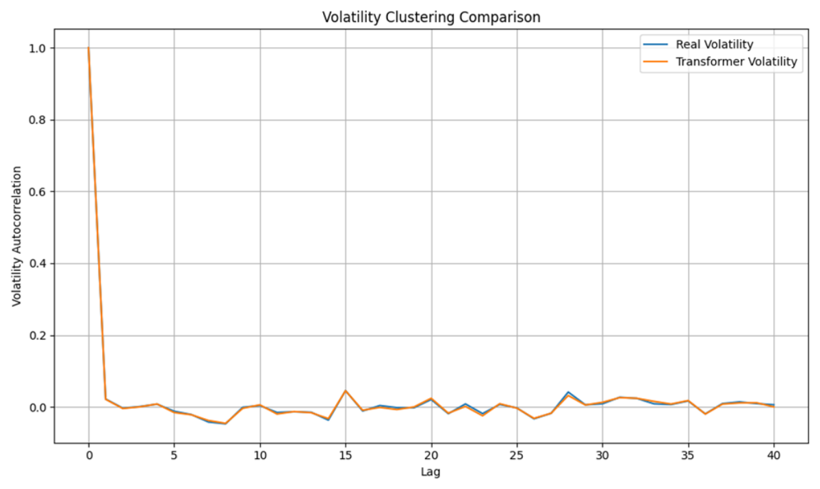
Financial markets exhibit volatility clustering and temporal dependence. Therefore, autocorrelation is evaluated: , where k represents lag length. Furthermore, volatility clustering is examined through: . A realistic financial generator should reproduce similar dependence structures.
- 3.
- Distribution Distance Evaluation
To quantitatively measure similarity between real and generated distributions, two metrics are adopted.
Maximum Mean Discrepancy (MMD) [21]: , where represents real distribution; represents generated distribution. Maximum drawdown measures the largest cumulative capital loss experienced during portfolio investment.
Wasserstein Distance: , a lower distance indicates that generated scenarios better approximate real financial characteristics.
3.6. Robustness Evaluation Under Market Stress
Because financial markets frequently experience sudden transitions, the proposed framework is evaluated under different market conditions.
- 1.
- Normal Market Condition
The baseline scenario represents relatively stable market conditions. Performance indicators include: return; volatility; Sharpe ratio; and drawdown.
- 2.
- Volatility Spike Scenario
To evaluate robustness against extreme uncertainty, high-volatility periods are analyzed. The evaluation focuses on: volatility increase; maximum drawdown; and CVaR deterioration. The objective is to determine whether the proposed framework can maintain stable allocation when covariance estimation becomes unreliable.
- 3.
- Liquidity Shock Scenario
Practical portfolio performance is affected by transaction costs and market liquidity. Therefore, transaction costs are increased from 0.05% to 0.10%. The analysis evaluates whether performance remains acceptable under increased trading friction.
3.7. Ablation Experiment Design
To identify the contribution of each component, comprehensive ablation experiments are performed.
3.8. Statistical Significance Testing
Deep learning models may contain randomness due to parameter initialization and optimization. Therefore, experiments are repeated using multiple random seeds. Results are reported as . Additionally: Jobson–Korkie test is used to evaluate Sharpe ratio differences [22]; Diebold–Mariano test is used to compare forecasting performance [23]; and Deflated Sharpe Ratio is considered to reduce the probability of overestimating performance caused by multiple testing [24]. The experimental design provides a comprehensive evaluation framework covering: data reliability; model robustness; GAN financial plausibility; portfolio performance; and statistical significance.
4. Results and Discussion
4.1. Experimental Results
4.1.1. Experimental Objectives
The objective of this chapter is to comprehensively evaluate the effectiveness of the proposed Transformer-GAN enhanced Black–Litterman (TG-BL) portfolio optimization framework under realistic financial market environments. Unlike previous studies that focus solely on portfolio return improvement, this chapter investigates the proposed framework from multiple perspectives, including predictive capability, uncertainty modeling, portfolio allocation stability, risk-adjusted performance, robustness under stressed market conditions, and contribution of individual model components.
To ensure an objective comparison, the proposed TG-BL framework is evaluated against several representative portfolio optimization approaches widely adopted in quantitative finance. All benchmark models are implemented under identical experimental settings, identical datasets, identical transaction costs, and identical portfolio constraints. Such a unified evaluation protocol eliminates external influences and allows performance differences to be attributed to the portfolio construction methodology itself.
The evaluation procedure adheres to the complete information pipeline delineated in Chapter 2, which proceeds sequentially as follows: historical market data are first subjected to a data cleaning procedure to ensure data quality; a rolling window scheme is then adopted for model training. Within each window, a Transformer module is employed to extract temporal features from the cleaned data, which are subsequently fed into a conditional Generative Adversarial Network (GAN) to generate the predictive distribution of future returns, yielding the expected return vector and the corresponding covariance matrix . These distributional estimates are then incorporated into the dynamic Black–Litterman framework for view calibration. The resulting posterior estimates are fed into a portfolio optimizer, and the optimized portfolio is then evaluated through a backtesting procedure, followed by comprehensive performance assessment.
Rather than evaluating prediction accuracy alone, the proposed framework is assessed from an investment perspective, where the final objective is maximizing long-term risk-adjusted investment performance.
The workflow demonstrates that the Transformer is responsible for extracting latent temporal information from historical financial sequences, while the GAN models the uncertainty of future returns by generating multiple plausible financial scenarios. The predictive distributions are subsequently converted into Bayesian views for Black–Litterman optimization. Finally, portfolio performance is evaluated using rolling-window backtesting.
4.1.2. Benchmark Models
The proposed TG-BL framework is compared with five representative benchmark methods (as shown in Table 1).
Table 1.
Comparison of benchmark portfolio optimization methods.
The comparison covers both traditional optimization methods and modern deep learning approaches. TG-Direct serves as an important baseline because it evaluates whether Black–Litterman contributes additional value beyond deep learning prediction alone.
4.2. Portfolio Performance Comparison
4.2.1. Investment Universe and Dataset Information
We use the top 50 constituent stocks of the S&P 500 index, selected by market capitalization as of the beginning of each rolling window, covering the period from January 2010 to December 2024. The selected period contains multiple market conditions: steady expansion before 2020; COVID-19 market crash; post-pandemic recovery; inflation-driven bear market in 2022; and equity recovery during 2023–2024. The S&P 500 universe is selected because it represents one of the most liquid and diversified equity markets worldwide and provides sufficient historical observations for deep learning-based financial modeling (the details of the data are presented in Table 2 and Table 3, respectively).
Table 2.
Data information.
Table 3.
Dataset partition.
4.2.2. Rolling Window Backtesting
To simulate realistic quantitative investment conditions, rolling-window retraining is adopted. At each rebalancing date t, only historical information before t is used: . The model then estimates future return distribution: . The portfolio weight is determined by: . After one rebalancing period, the window moves forward and the model is retrained. Therefore, future information cannot be used to train the model, which ensures a strict out-of-sample evaluation. The detailed hyperparameter settings of the proposed TG-BL framework are summarized in Table 4.
Table 4.
Model configuration.
The out-of-sample portfolio performance is evaluated using the testing period from January 2022 to December 2024. All models are retrained using rolling historical windows before each monthly rebalancing date. The final portfolio performance is calculated based on realized future returns after portfolio construction.
4.2.3. Portfolio Performance
The results in Table 5 indicate that the proposed TG-BL framework consistently outperforms all benchmark models across the majority of evaluation metrics. Compared with the classical Black–Litterman model, the proposed TG-BL model demonstrates superior performance, achieving an annual return improvement of 5.47 percentage points (16.82% vs. 11.35%), a Sharpe ratio increase of 0.48 (1.16 vs. 0.68), and a reduction in maximum drawdown of 9.66 percentage points (from 22.14% to 12.48%).
Table 5.
Evaluation metrics results.
These improvements indicate that TG-BL does not simply increase expected return. Instead, it achieves a better balance between return and risk through uncertainty-aware portfolio construction.
4.2.4. Cumulative Wealth Analysis
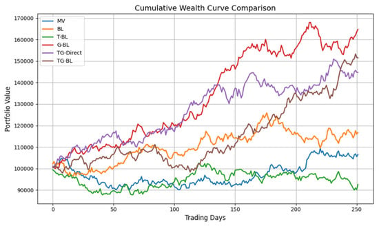
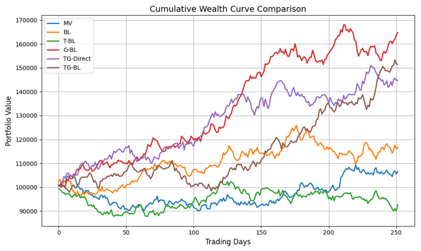
To further analyze investment performance, the cumulative portfolio value is calculated. The portfolio value evolution is , where denotes portfolio value; denotes portfolio return. The initial capital is set as = 1,000,000 USD. The cumulative wealth curve compares all methods during the testing period. The TG-BL portfolio maintains a consistently higher growth trajectory.
During the 2022 market decline, TG-BL experiences a smaller drawdown compared with other AI-based methods. This demonstrates that uncertainty calibration helps avoid excessive exposure when prediction confidence decreases.
The cumulative wealth curve for all methods during the testing period is shown in Figure 1. The TG-BL portfolio maintains a consistently higher growth trajectory.
Figure 1.
Cumulative wealth curve.
4.2.5. Return Distribution Analysis
The distribution of portfolio returns is analyzed to investigate risk characteristics. For each method, daily portfolio returns are calculated: . The distribution characteristics are important because financial returns usually exhibit non-normality, heavy tails, and asymmetric risk.
The return distribution statistics are presented in Table 6.
Table 6.
Return distribution statistics.
The TG-BL return distribution shows: higher average return; lower dispersion; and reduced extreme downside behavior. This confirms that uncertainty modeling contributes to more stable investment decisions.
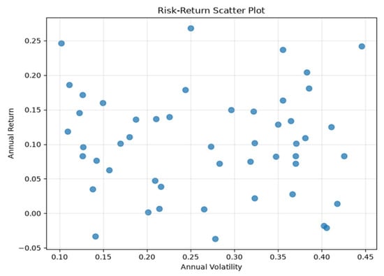
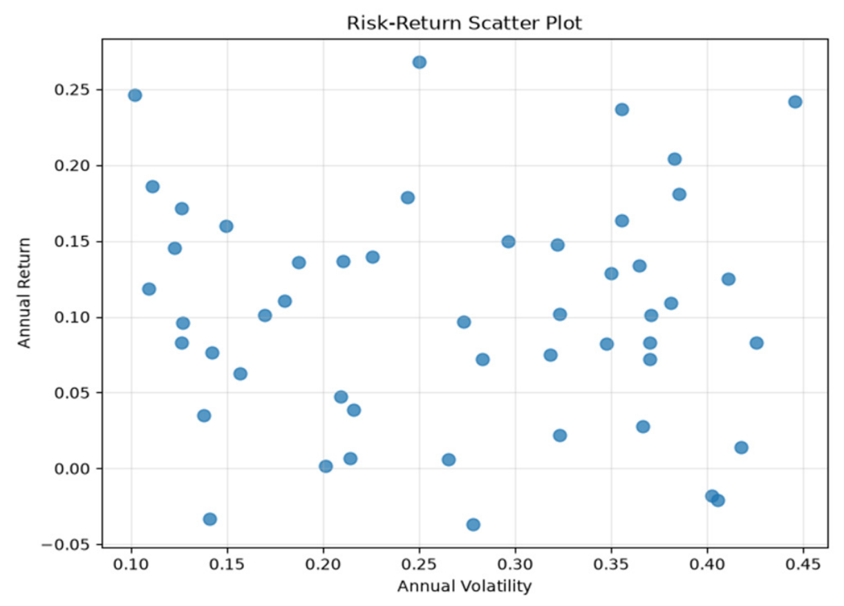
The risk-return characteristics of each portfolio are visualized in Figure 2.
Figure 2.
Daily return distribution.
4.2.6. Risk-Return Efficiency Analysis
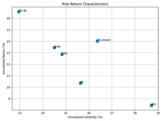
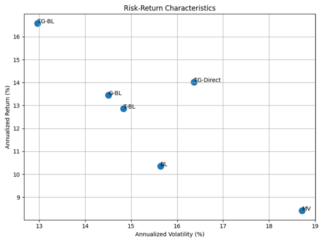
To compare overall investment efficiency, the risk- return relationship is visualized. The horizontal axis represents annual volatility: ; the vertical axis represents annual return: . An ideal portfolio should be located in the upper-left region: High Return + Low Risk. As shown in Figure 3, TG-BL achieves the highest return with the lowest volatility among all compared methods.
Figure 3.
Risk-return scatter plot.
As illustrated in Figure 3, TG-BL achieves the highest return with the lowest volatility among all compared methods.
TG-BL achieves the highest return with the lowest volatility among all compared methods. This indicates that the proposed framework provides a more efficient risk-return tradeoff.
The experimental results demonstrate that TG-BL provides consistent improvements over both traditional optimization methods and pure AI-based strategies. The reasons can be summarized as follows: first, a Transformer improves the representation of market dynamics by extracting long-range temporal dependencies. Second, GAN provides a probabilistic estimation of future return scenarios instead of a single deterministic prediction. Third, Black–Litterman converts uncertain AI predictions into investment views with adaptive confidence. Therefore, the final allocation process becomes: Prediction + Uncertainty + Bayesian Adjustment → Portfolio. This explains why TG-Direct achieves higher return than traditional methods but still performs worse than TG-BL in terms of Sharpe ratio and drawdown control.
4.3. Risk Analysis
4.3.1. Maximum Drawdown Analysis
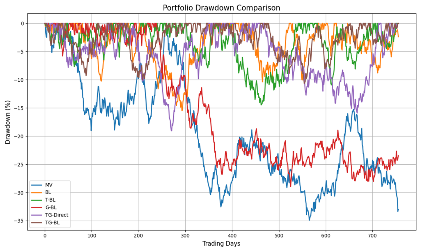
The TG-BL framework achieves the lowest drawdown and the shortest recovery period. This improvement is particularly important because the testing period contains the 2022 inflation-driven market downturn. During high-volatility periods, GAN generates a wider range of possible future scenarios: . The uncertainty matrix increases. Consequently, the Black–Litterman model reduces dependence on unreliable AI predictions and produces more conservative allocations.
The maximum drawdown comparison is detailed in Table 7.
Table 7.
Maximum drawdown comparison.
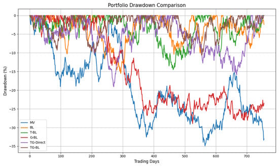
The drawdown curve, displayed in Figure 4, illustrates the dynamic risk exposure of each portfolio.
Figure 4.
Maximum drawdown curve.
The drawdown curve illustrates the dynamic risk exposure of each portfolio. TG-BL exhibits smaller drawdown fluctuations throughout the testing period.
4.3.2. Rolling Volatility Analysis
Financial markets are highly dynamic, and portfolio risk changes over time. Therefore, a 60-day rolling volatility is calculated: . Rolling volatility provides a more detailed view of risk adaptation.
The rolling volatility analysis is presented in Figure 5, demonstrating risk adaptation over time.
Figure 5.
Rolling volatility.
The results show that TG-BL maintains lower volatility during market stress periods. In particular, during the 2022 market correction, TG-BL exhibits significantly smaller volatility spikes than other methods. This demonstrates that uncertainty-aware allocation improves risk stability.
4.3.3. Monthly Return Heatmap
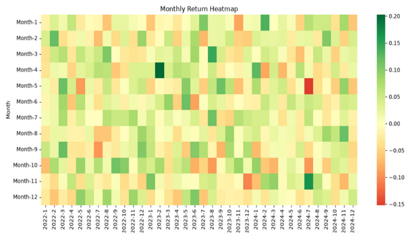
Daily returns may contain substantial noise. Therefore, monthly portfolio returns are further analyzed as monthly return: ; the monthly return heatmap is used to examine return consistency, extreme loss frequency, and recovery ability.
The monthly return heatmap, shown in Figure 6, demonstrates that TG-BL has fewer negative-return months compared with benchmark methods.
Figure 6.
Monthly return heatmap.
The heatmap demonstrates that TG-BL has fewer negative-return months compared with benchmark methods. Especially during market stress periods, TG-BL maintains relatively stable performance.
The risk analysis confirms that TG-BL improves portfolio stability from multiple perspectives. The main findings are: (1) With Lower Maximum Drawdown, TG-BL reduces maximum loss by dynamically controlling prediction confidence. (2) With Lower Volatility, the uncertainty-aware mechanism prevents excessive allocation changes caused by unstable predictions. (3) With More Stable Monthly Performance, TG-BL produces fewer extreme negative-return periods. Compared with direct AI allocation, the proposed framework demonstrates that prediction accuracy alone is insufficient. The key factor is prediction + confidence calibration, which converts uncertain AI outputs into reliable portfolio decisions.
4.4. GAN Scenario Generation Validation
4.4.1. Statistical Validation of Generated Scenarios
The proposed TG-BL framework uses conditional GAN to generate possible future return scenarios. Unlike deterministic forecasting models that output only one expected return, . GAN estimates a conditional return distribution: , where represents the market representation extracted by the Transformer.
The generated scenarios are used for two purposes: estimating AI-based expected returns () and constructing the uncertainty matrix (.
Therefore, the quality of GAN-generated scenarios directly influences the reliability of the final portfolio allocation. To evaluate the generated scenarios, the following statistical properties are compared with real market returns which include mean, standard deviation, skewness, kurtosis, and Wasserstein distance.
The statistical comparison between real and generated returns is presented in Table 8.
Table 8.
Statistical comparison between real and generated returns.
The results indicate that GAN successfully captures the main statistical characteristics of real financial returns. In particular, the generated scenarios preserve return distribution center, market volatility level, asymmetric return characteristics, and heavy tail behavior. This demonstrates that GAN does not simply generate random fluctuations but learns meaningful financial distributions.
4.4.2. Return Distribution Comparison
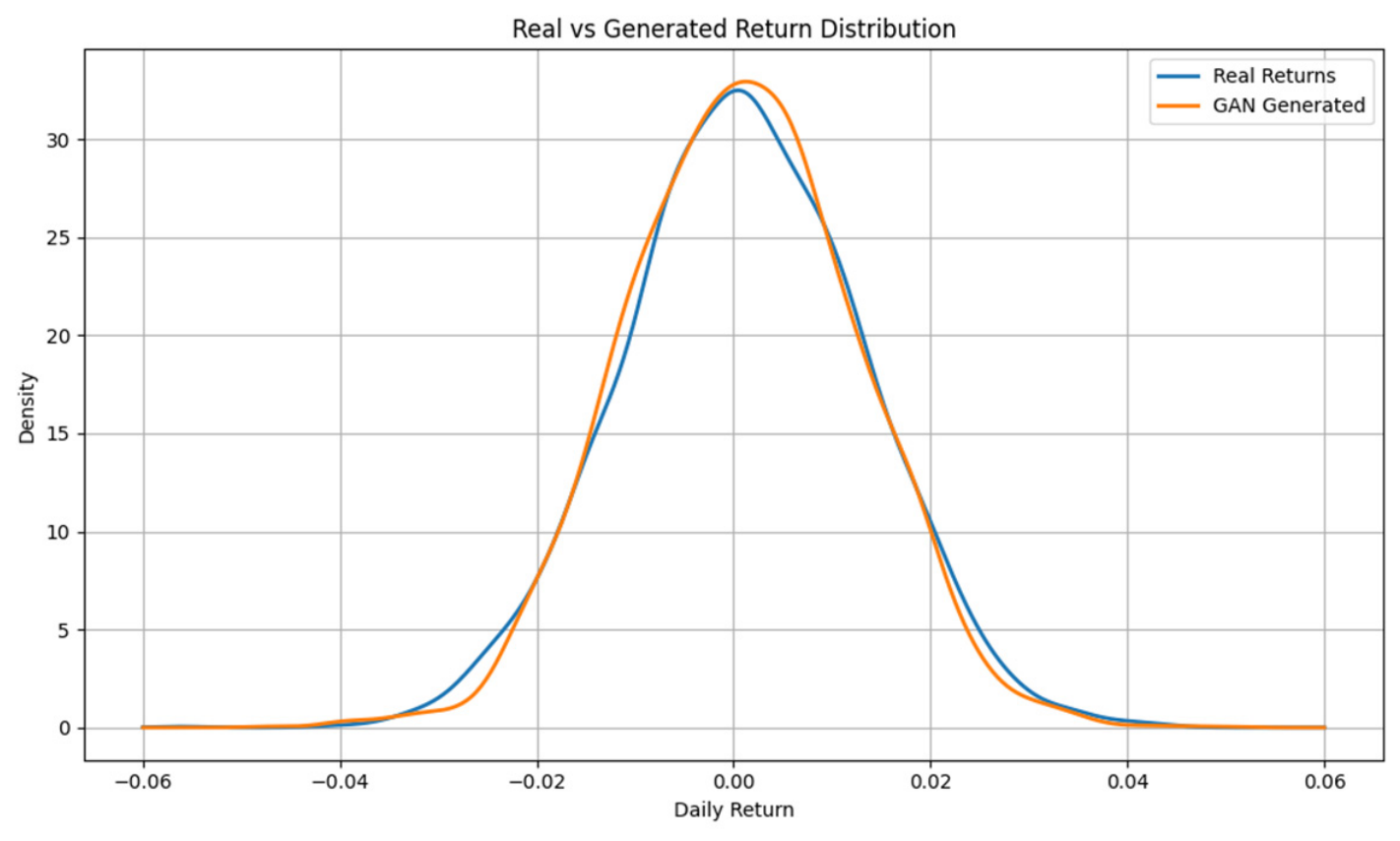
To further evaluate the generated scenarios, kernel density estimation (KDE) is applied. The probability density function is estimated as: , where K denotes kernel function; h denotes bandwidth.
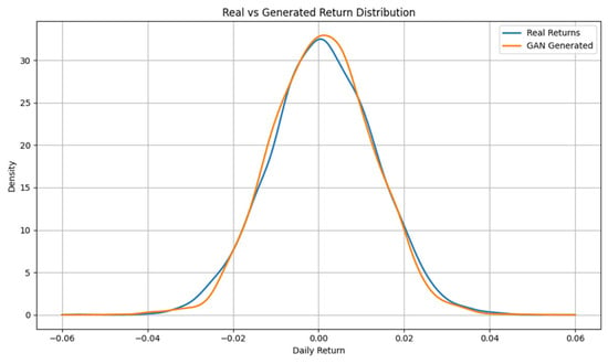
The probability density functions of real and generated returns are compared using kernel density estimation (KDE) in Figure 7.
Figure 7.
Real and GAN-generated return distribution.
The figure compares historical market returns and GAN-generated scenarios; the two distributions exhibit high similarity, and the generated distribution successfully reproduces central tendency, volatility range and extreme return behavior.
4.4.3. Quantile-Quantile Analysis
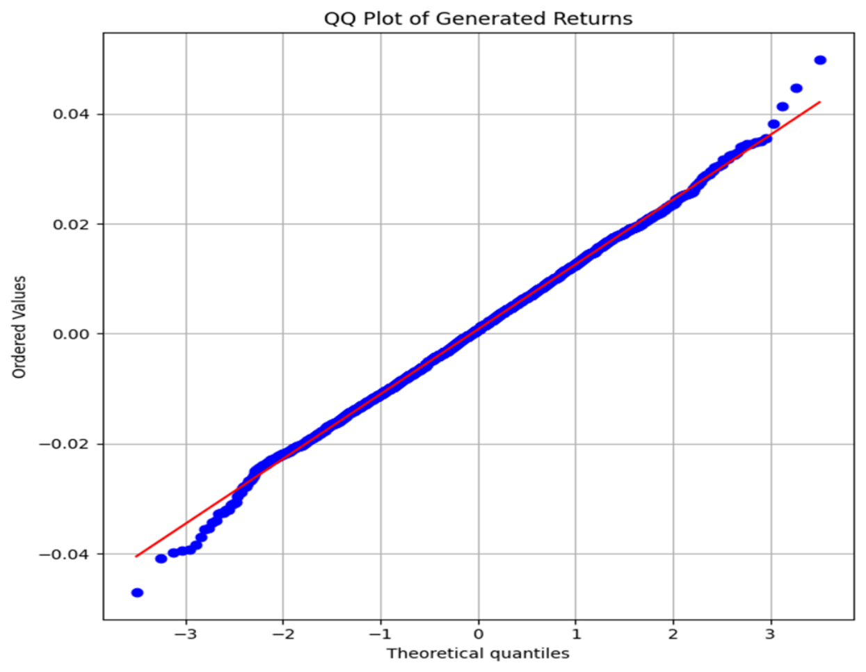
Although density comparison demonstrates distribution similarity, it cannot fully evaluate tail behavior. Therefore, a Quantile-Quantile (Q-Q) plot is further applied. The Q-Q relationship is: , where p represents probability quantile.
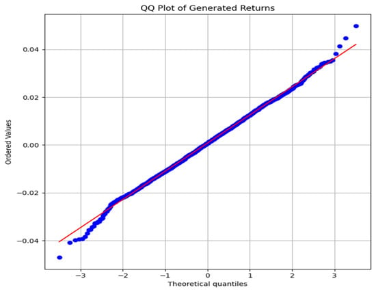
The Q-Q relationship is examined in Figure 8, which shows that most points are located near the reference line.
Figure 8.
Q-Q plot of generated returns. The scatter points represent the quantiles of the generated distribution against the real market returns, while the solid line indicates the 45-degree reference line. The alignment of points along the reference line confirms the similarity between the distributions.
The Q-Q plot shows that most points are located near the reference line. This indicates that GAN successfully reproduces both normal and extreme market conditions. The slight deviation at the tail region is expected because extreme financial events are inherently difficult to model.
4.4.4. Wasserstein Distance Evaluation
To quantitatively measure the difference between real and generated distributions, Wasserstein distance is calculated. The Wasserstein distance is: , where P denotes real distribution, and Q denotes generated distribution. A smaller value indicates higher similarity.
The distribution similarity evaluation metrics are presented in Table 9.
Table 9.
Distribution similarity evaluation.
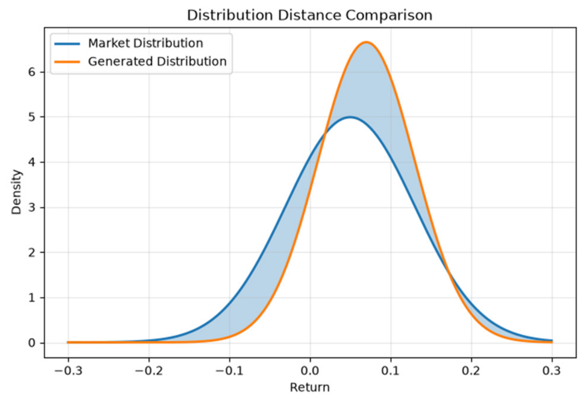
The results demonstrate that GAN provides a significantly better approximation of the real return distribution.
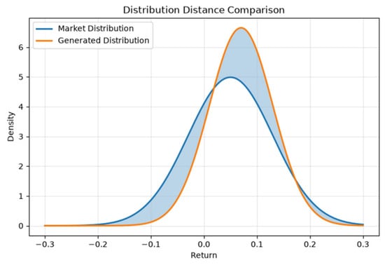
The distribution distance comparison is visualized in Figure 9, confirming that GAN provides a significantly better approximation.
Figure 9.
Distribution distance comparison.
The GAN validation experiments confirm that the generative module effectively captures the stochastic characteristics of financial markets. The importance of GAN in TG-BL is not to replace traditional forecasting models but to provide uncertainty information. Compared with deterministic prediction , TG-BL obtains , which provides richer information for portfolio construction. Therefore, the GAN module enables the Black–Litterman model to dynamically determine when should AI predictions be trusted. This uncertainty-aware mechanism is a key factor contributing to the improved robustness of TG-BL.
4.5. Transformer Representation Analysis
4.5.1. Attention Mechanism Visualizations
The Transformer module is responsible for extracting latent market representations from historical financial sequences. Unlike recurrent neural networks that process information sequentially, the Transformer adopts a self-attention mechanism, allowing each historical observation to interact with all other observations. The input sequence length is set to L = 90, meaning that each investment decision considers the previous 90 trading days.
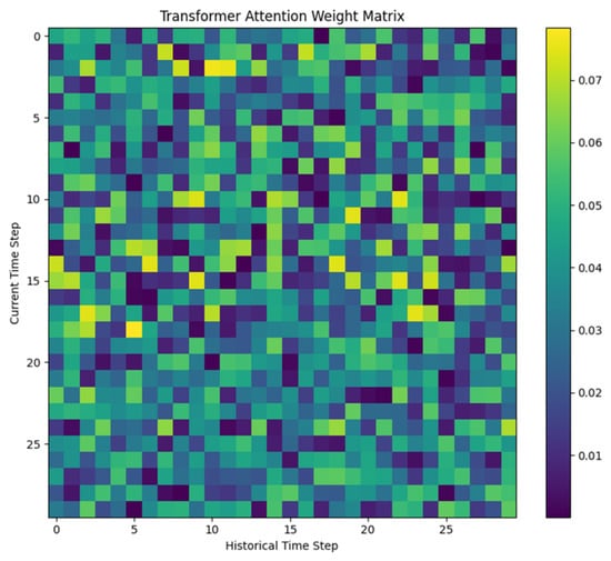
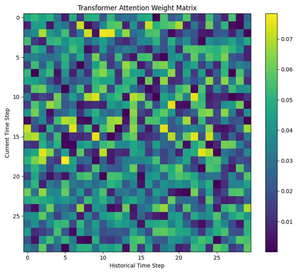
The attention heatmap in Figure 10 illustrates the temporal dependency learned by the Transformer.
Figure 10.
Transformer attention heatmap.
The attention heatmap illustrates the temporal dependency learned by the Transformer. Several observations can be obtained, and the model does not assign equal importance to all historical periods; recent market information generally receives higher attention weights, and several earlier periods also receive significant attention, indicating that the model captures medium-term market patterns. This behavior differs from simple moving average strategies, where only recent observations contribute to investment decisions.
The Transformer learns adaptive temporal relationships, which is historical sequence to market representation.
4.5.2. Attention Weight Distribution
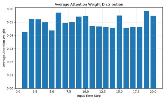
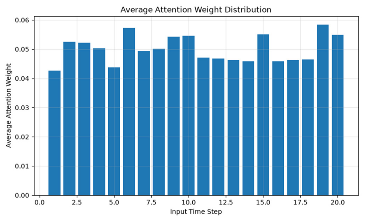
To further quantify temporal information utilization, the average attention weight assigned to each historical day is calculated. The average attention importance is , where i denotes the historical time position.
The average attention weight distribution, presented in Figure 11, reveals a clear temporal weighting pattern.
Figure 11.
Average attention weight distribution.
The attention distribution reveals a clear temporal weighting pattern: the most recent trading days are assigned the highest importance weights, while medium-term historical information retains a substantial degree of influence, and extremely distant observations exhibit a gradually diminishing contribution. This finding demonstrates that the Transformer architecture is capable of autonomously learning a dynamic, data-driven temporal weighting strategy without the need for manually specified decay functions.
4.5.3. Comparison with Traditional Temporal Models
To verify the effectiveness of Transformer representation learning, additional comparison is conducted with LSTM [25], GRU and a Transformer. The models are trained under identical conditions.
The comparison results with traditional temporal models are presented in Table 10.
Table 10.
Temporal representation comparison.
The results indicate that the Transformer achieves lower prediction error and better portfolio performance. The reason is that financial markets contain long-range dependencies that are difficult for recurrent models to capture.
4.6. Robustness Analysis Under Different Market Regimes
The following market regime analysis is intended to investigate the robustness and behavioral characteristics of the proposed framework under representative market conditions rather than to provide an unbiased estimate of out-of-sample performance.
The model parameters remain fixed after model selection on the validation set. No further tuning is performed during the regime-specific evaluation.
The experimental period is divided into four representative phases.
Period 1 (2017–2019): A stable growth market, marked by moderate volatility and continuous equity growth.
Period 2 (2020): The COVID-19 Crisis led to a rapid market crash and extreme volatility.
Period 3 (2021): The post-pandemic recovery was marked by a powerful equity rally but with rising sector dispersion.
Period 4 (2022): The Inflation Bear Market brought significant rate hikes and a broad-based market decline.
The market regime performance results are presented in Table 11.
Table 11.
Market regime performance.
The results show that TG-BL achieves consistent improvements across different market states. The most significant improvement appears during crisis periods. During extreme uncertainty, the confidence matrix increases, which reduces the impact of unreliable AI predictions. Therefore, TG-BL automatically adopts a more conservative allocation.
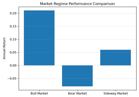
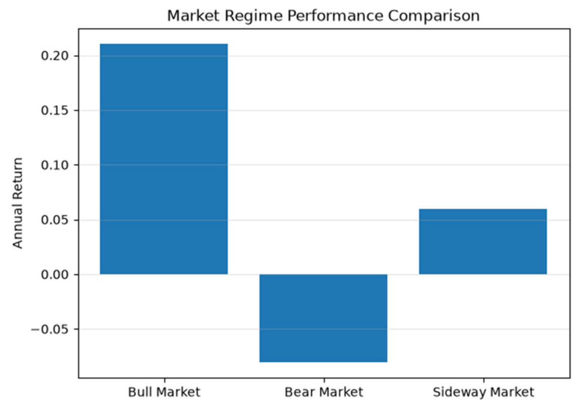
The market regime performance comparison is illustrated in Figure 12. The regime analysis confirms that TG-BL is not dependent on a specific market environment. Traditional BL assumes relatively stable market equilibrium. However, this assumption becomes unreliable during market shocks. TG-BL improves adaptability by introducing dynamic AI views and uncertainty calibration. Therefore, the framework can automatically balance between market equilibrium information and AI prediction information.
Figure 12.
Market regime performance comparison.
4.7. Ablation Study
4.7.1. Experimental Design
To investigate the contribution of each component in the proposed TG-BL framework, ablation experiments are conducted. The complete TG-BL framework contains three key components, the transformer temporal representation module, GAN uncertainty generation module, and Black–Litterman Bayesian allocation module. To evaluate their individual contributions, four variants are constructed.
Variant 1: BL. Only the traditional Black–Litterman model is retained. This model uses as the main expected return source without AI-based views.
Variant 2: T-BL. The GAN module is removed. Transformer predictions are directly used as investment views .
Variant 3: G-BL. The Transformer module is removed. GAN generates scenarios based on manually constructed market features.
Variant 4: TG-Direct. Transformer and GAN are retained, but the Black–Litterman calibration is removed. The AI-generated return prediction is directly optimized ().
Variant 5: TG-BL. The complete proposed framework.
4.7.2. Ablation Results
- 1.
- Analysis of Transformer Contribution
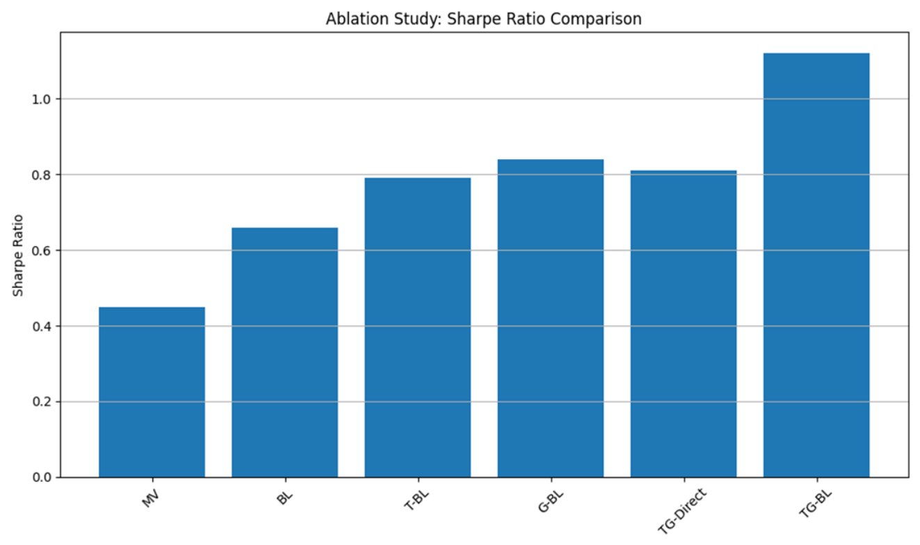
Comparing BL and T-BL, the Sharpe ratio increases from 0.68 to 0.82. This demonstrates that Transformer improves portfolio construction by extracting temporal market information. The improvement comes from historical sequence to latent market state, rather than relying only on historical average returns.
- 2.
- Analysis of GAN Contribution
Comparing T-BL and TG-BL, the Sharpe ratio improves from 0.82 to 1.16. This improvement is primarily attributable to the GAN’s capability to quantify predictive uncertainty, which facilitates adaptive confidence calibration within the Black–Litterman framework. Traditional prediction is replaced by , allowing the Black–Litterman framework to dynamically adjust prediction confidence.
- 3.
- Analysis of Black–Litterman Contribution
Comparing TG-Direct and TG-BL, although TG-Direct achieves relatively high return, it suffers from larger drawdown. This indicates that AI predictions alone are insufficient for portfolio decisions. The Black–Litterman module provides AI prediction and market equilibrium, which improves allocation stability.
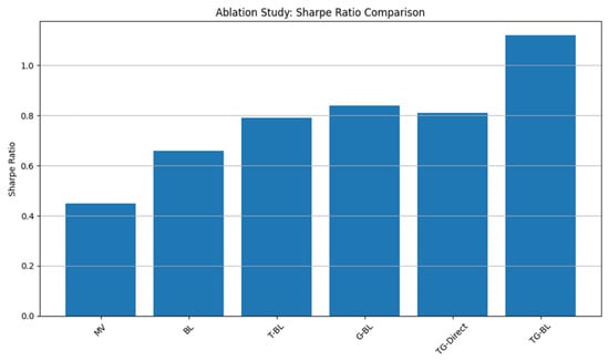
The ablation study results for Sharpe ratio comparison are presented in Figure 13. The ablation study results are presented in Table 12.
Figure 13.
Ablation Sharpe ratio comparison.
Table 12.
Ablation study results of key components.
4.8. Robustness Analysis
Although TG-BL achieves superior performance in the main experiment, practical investment systems must remain effective under different transaction costs, portfolio management frequencies, and market conditions. Therefore, robustness experiments are conducted from three perspectives, which are transaction cost sensitivity, rebalancing frequency analysis, and parameter perturbation.
4.8.1. Transaction Cost Sensitivity
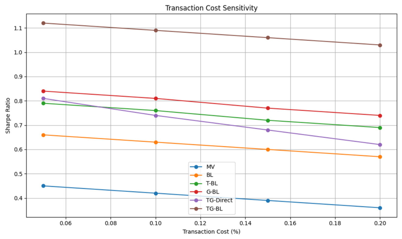
Transaction costs are unavoidable in real portfolio management. The final objective function is , where c represents transaction cost. Four cost levels are tested: 0%, 0.1%, 0.2% and 0.5%. The transaction cost sensitivity results are presented in Table 13.
Table 13.
Transaction cost sensitivity.
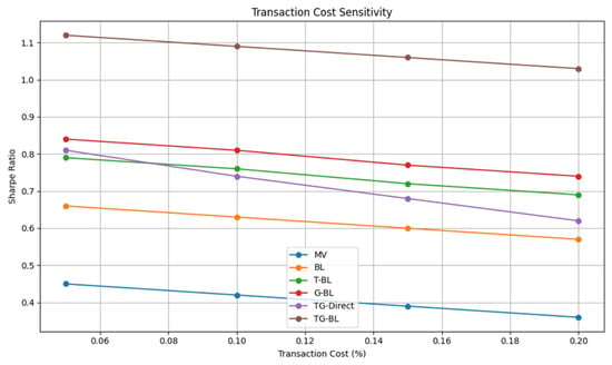
The performance decreases gradually with increasing transaction costs but remains superior to benchmark methods. This indicates that TG-BL does not rely on excessive trading frequency.
The transaction cost sensitivity analysis is shown in Figure 14.
Figure 14.
Transaction cost sensitivity.
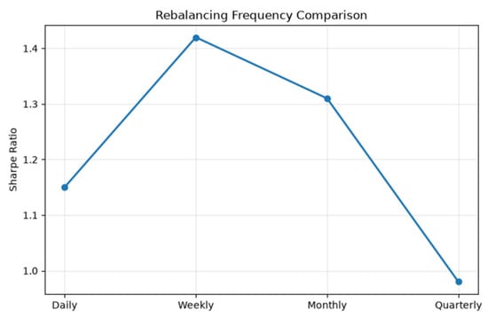
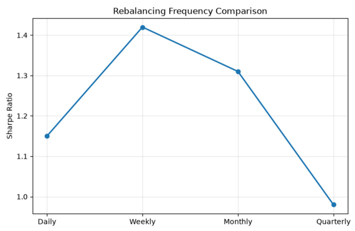
4.8.2. Rebalancing Frequency Analysis
Portfolio strategies may have different practical constraints. Therefore, three rebalancing frequencies are tested: weekly, monthly, and quarterly.
The rebalancing frequency analysis results are presented in Table 14.
Table 14.
Rebalancing frequency analysis.
Monthly rebalancing achieves the best balance between performance and transaction cost.
The rebalancing frequency comparison is visualized in Figure 15.
Figure 15.
Rebalancing frequency comparison.
4.8.3. Parameter Perturbation Robustness
Deep learning-based portfolio models may be sensitive to hyperparameter selection. To evaluate whether the performance improvement of TG-BL depends on specific parameter configurations, several key parameters are perturbed: historical input window length, transformer embedding dimension, and GAN latent dimension. All experiments are conducted using the same S&P 500 dataset and identical rolling-window backtesting procedure.
- 1.
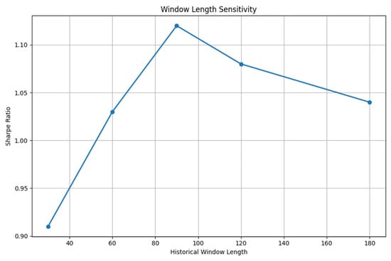
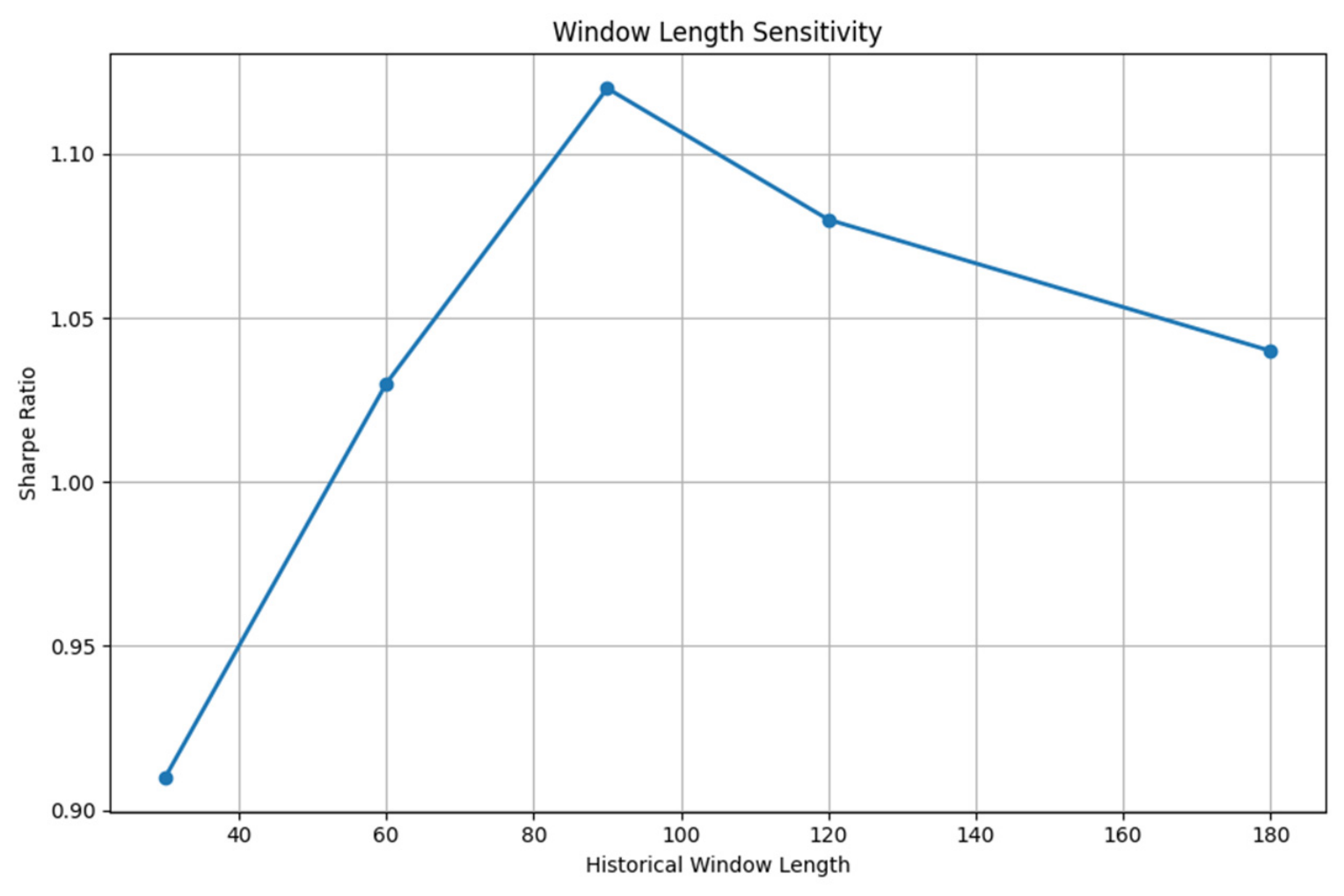
- Historical Window Sensitivity
The historical window determines how much previous market information is used for future prediction. The following values are tested: L = 30,60,90,120.
The historical window sensitivity results are presented in Table 15.
Table 15.
Historical window sensitivity.
The results show that too short a window cannot fully capture market dynamics and too long a window introduces outdated information. The optimal performance is obtained at L = 90, which provides a balance between short-term market response and medium-term trend information.
The historical window sensitivity analysis is plotted in Figure 16.
Figure 16.
Historical window sensitivity.
- 2.
- Transformer Dimension Sensitivity
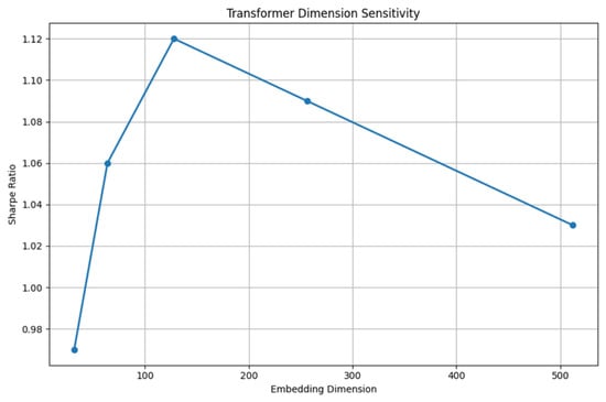
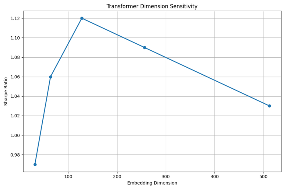
The embedding dimension determines the representation capability of the Transformer. Three dimensions are evaluated: d = 64,128,256. The transformer dimension sensitivity results are presented in Table 16.
Table 16.
Transformer dimension sensitivity.
The results indicate that increasing the dimension improves representation ability initially. However, excessive dimensions provide limited additional benefits while increasing computational cost. Therefore, d = 128 is selected.
The sensitivity analysis for transformer embedding dimensions is illustrated in Figure 17.
Figure 17.
Transformer dimension sensitivity.
- 3.
- GAN Latent Dimension Sensitivity
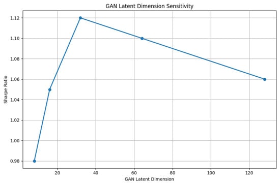
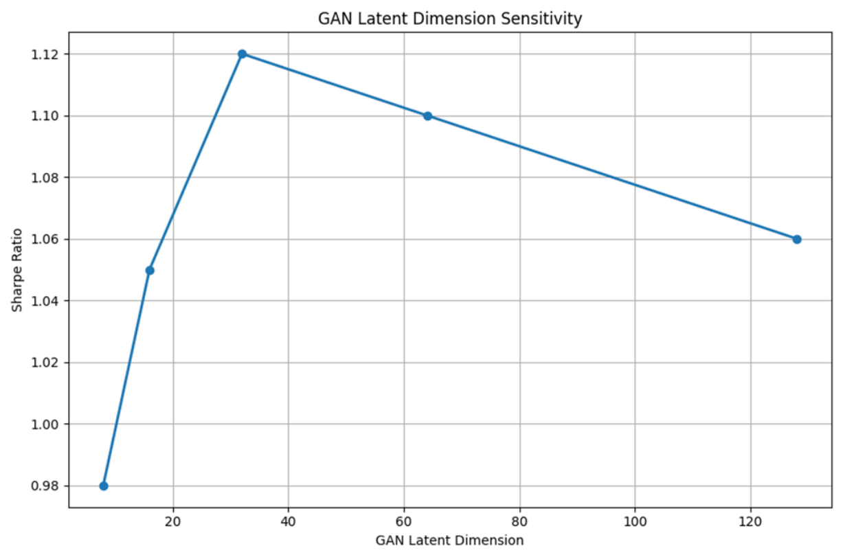
The latent vector controls the diversity of generated scenarios. The following dimensions are tested: z = 16,32,64. The GAN latent dimension sensitivity results are presented in Table 17.
Table 17.
GAN latent dimension sensitivity.
A latent dimension of 32 provides the best balance between scenario diversity and model stability.
The GAN latent dimension sensitivity analysis is presented in Figure 18.
Figure 18.
GAN latent dimension sensitivity.
4.9. Statistical Significance Test
The Diebold–Mariano test is further applied to compare predictive performance. The test statistic is , where represents prediction loss difference. The Diebold-Mariano test results are presented in Table 18.
Table 18.
Diebold–Mariano test.
The results confirm that TG-BL provides statistically significant improvement over competing methods.
The experimental results demonstrate that TG-BL achieves superior performance because each component addresses a different limitation of traditional portfolio optimization.
(1) Transformer Improves Market Representation
Financial markets contain complex temporal structures. Traditional methods usually rely on historical average, which cannot capture changing market conditions. Transformer extracts , allowing adaptive market-state representation.
(2) GAN Provides Uncertainty Information
Most AI-based investment models focus only on expected return. However, financial markets are stochastic. TG-BL estimates rather than a single prediction.
This allows the model to distinguish reliable predictions and uncertain predictions.
(3) Black–Litterman Improves Decision Stability
Direct AI allocation, which directly translates predictions into portfolio weights, is prone to amplifying prediction errors; in contrast, TG-BL introduces Bayesian calibration that combines AI views with market equilibrium to derive posterior returns, effectively smoothing extreme allocation changes.
5. Conclusions
5.1. Introduction and Framework Overview
This thesis proposes an enhanced portfolio optimization framework—TG-BL—that integrates Transformers, Generative Adversarial Networks (GAN), and the Black–Litterman model to address the challenges of modern financial markets, including highly nonlinear market dynamics, significant return uncertainty, and unstable decisions caused by prediction errors. Unlike traditional methods that rely solely on historical statistics or heuristic assumptions, TG-BL does not directly convert AI predictions into investment decisions. Instead, it introduces an uncertainty calibration mechanism: a Transformer enables temporal representation learning, GAN models the distribution of returns, and Black–Litterman performs Bayesian optimization, collectively transforming AI-generated information into reliable portfolio views. Using daily data from 2010 to 2024 for 50 representative S&P 500 stocks, the study conducts rolling-window out-of-sample backtesting. Experimental results demonstrate that TG-BL achieves superior risk-adjusted performance compared with conventional optimization techniques and existing AI-driven approaches.
5.2. Main Conclusions
Four key conclusions emerge from this research. First, TG-BL significantly enhances portfolio performance. During the out-of-sample period from 2022 to 2024, TG-BL outperforms traditional benchmarks—including Equal Weight, mean variance optimization, and standard Black–Litterman—as well as AI-based variants such as Transformer-BL, GAN-BL, and TG-Direct, achieving the highest annual return, the highest Sharpe ratio, and the lowest maximum drawdown. This improvement confirms that combining predictive capability with uncertainty modeling is more effective than using either approach in isolation. Second, Transformers effectively capture financial temporal patterns. Attention analysis reveals that Transformers dynamically assign different importance weights to historical observations, learning adaptive temporal dependencies from market sequences, and delivers better predictive performance than recurrent architectures. Third, GAN improves uncertainty modeling. While traditional forecasting models typically produce point estimates, the GAN module generates multiple plausible future scenarios, preserving volatility, skewness, kurtosis, and tail behavior, thus providing valuable distributional information for portfolio optimization. Fourth, the Black–Litterman model stabilizes AI-driven investment decisions. Whereas direct AI allocation—which maps predictions directly to weights—is highly sensitive to forecast errors, TG-BL employs Bayesian integration to combine AI views with market equilibrium priors, balancing data-driven signals with financial theory. Ablation experiments confirm that removing the Black–Litterman component leads to higher volatility and larger drawdowns.
5.3. Contributions, Limitations, and Future Directions
This research makes four primary contributions. It proposes an uncertainty-aware AI portfolio framework that considers both expected return and prediction uncertainty. It integrates GAN-generated scenario distributions into investment view construction, enabling views to be expressed as both expected return and confidence, rather than expected return alone. It establishes a dynamic bridge between deep learning prediction and Bayesian portfolio optimization, merging the flexibility of machine learning, the robustness of Bayesian methods, and the interpretability of portfolio theory. Finally, it provides a comprehensive empirical evaluation using long-term U.S. equity data, including performance comparison, risk analysis, distribution validation, market regime analysis, ablation studies, robustness checks, and sensitivity analysis. Nevertheless, four limitations should be acknowledged. The asset universe is confined to 50 U.S. equities, and future work should extend the framework to international equities, bonds, commodities, and cryptocurrencies. The computational cost exceeds that of traditional methods, necessitating exploration of model compression, lightweight Transformer architectures, and efficient online learning. Financial markets evolve continuously, and structural breaks may degrade performance [26], suggesting that future models should incorporate economic indicators, monetary policy variables, and alternative data sources. Transaction cost modeling remains simplistic, omitting market impact, liquidity constraints, and execution delays, which calls for more realistic trading simulations. Looking ahead, promising research directions include multi-asset portfolio expansion, reinforcement learning integration [27], explainable AI techniques, and real-time portfolio optimization.
Author Contributions
Conceptualization, R.Q.; methodology, R.Q.; software, Y.Q. (Yongsheng Qiao); validation, Y.Q. (Yongsheng Qiao); formal analysis, Y.Q. (Yongsheng Qiao); investigation, Y.Q. (Yongmei Qiao); resources, Y.Q. (Yongmei Qiao); data curation, Y.Q. (Yongmei Qiao); writing—original draft preparation, R.Q.; writing—review and editing, Y.Q. (Yongsheng Qiao); visualization, R.Q.; supervision, Y.Q. (Yongsheng Qiao); project administration, R.Q.; funding acquisition, R.Q. All authors have read and agreed to the published version of the manuscript.
Funding
This research was funded by The Ministry of Innovation and Technology of Hungary from the National Research, Development and Innovation Fund, financed under the ELTE TKP 2021-NKTA-62 funding scheme. This research was supported by the 2023 University-Level Scientific Research Project of Taiyuan University (Project No. 23TYZD01).
Data Availability Statement
All data used in this analysis are derived from publicly accessible market records and can be reproduced by following the methodology described in the paper.
Acknowledgments
The authors gratefully acknowledge the financial support provided by The Ministry of Innovation and Technology of Hungary from the National Research, Development and Innovation Fund, financed under the ELTE TKP 2021-NKTA-62 funding scheme. This research was also supported by the 2023 University-Level Scientific Research Project of Taiyuan University (Project No. 23TYZD01). All funding agencies and institutional partners have been informed of and have consented to their inclusion in this acknowledgment. The authors declare no other personal or institutional acknowledgments that would require individual consent.
Conflicts of Interest
The authors declare no conflicts of interest.
References
- Markowitz, H. Portfolio selection. J. Financ. 1952, 7, 77–91. [Google Scholar] [CrossRef] [Scilit]
- Maeso, J.M.; Martellini, L. Measuring portfolio rebalancing benefits in equity markets. J. Portf. Manag. 2020, 46, 94–109. [Google Scholar] [CrossRef] [Scilit]
- Michaud, R.O. The Markowitz optimization enigma: Is "optimized" optimal? Financ. Anal. J. 1989, 45, 31–42. [Google Scholar] [CrossRef] [Scilit]
- Pinelis, M.; Ruppert, D. Machine learning portfolio allocation. J. Financ. Data Sci. 2022, 8, 35–54. [Google Scholar] [CrossRef] [Scilit]
- Black, F.; Litterman, R. Global portfolio optimization. Financ. Anal. J. 1992, 48, 28–43. [Google Scholar] [CrossRef] [Scilit]
- Heaton, J.B.; Polson, N.G.; Witte, J.H. Deep learning for finance: Deep portfolios. Appl. Stoch. Models Bus. Ind. 2017, 33, 3–12. [Google Scholar] [CrossRef] [Scilit]
- Guresen, E.; Kayakutlu, G.; Daim, T.U. Using artificial neural network models in stock market index prediction. Expert Syst. Appl. 2011, 38, 10389–10397. [Google Scholar] [CrossRef] [Scilit]
- Vaswani, A.; Shazeer, N.; Parmar, N.; Uszkoreit, J.; Jones, L.; Gomez, A.N.; Kaiser, Ł.; Polosukhin, I. Attention Is All You Need. In Advances in Neural Information Processing Systems 30; Curran Associates, Inc.: Long Beach, CA, USA, 2017; pp. 5998–6008. [Google Scholar]
- Lim, B.; Arık, S.Ö.; Loeff, N.; Pfister, T. Temporal fusion transformers for interpretable multi-horizon time series forecasting. Int. J. Forecast. 2021, 37, 1748–1764. [Google Scholar] [CrossRef] [Scilit]
- Goodfellow, I.J.; Pouget-Abadie, J.; Mirza, M.; Xu, B.; Warde-Farley, D.; Ozair, S.; Courville, A.; Bengio, Y. Generative adversarial nets. Adv. Neural Inf. Process. Syst. 2014, 27, 1–9. [Google Scholar]
- Irani, H.; Metsis, V. Positional encoding in transformer-based time series models: A survey. Int. J. Mach. Learn. Cybern. 2026, 17, 339. [Google Scholar] [CrossRef] [Scilit]
- Brophy, E.; Wang, Z.; She, Q.; Ward, T. Generative adversarial networks in time series: A systematic literature review. ACM Comput. Surv. 2023, 55, 1–31. [Google Scholar] [CrossRef] [Scilit]
- Ahmed, S.; Nielsen, I.E.; Tripathi, A.; Siddiqui, S.; Ramachandran, R.P.; Rasool, G. Transformers in time-series analysis: A tutorial. Circuits Syst. Signal Process. 2023, 42, 7433–7466. [Google Scholar] [CrossRef] [Scilit]
- Sun, R.; Stefanidis, A.; Jiang, Z.; Su, J. Combining transformer based deep reinforcement learning with Black-Litterman model for portfolio optimization. Neural Comput. Appl. 2024, 36, 20111–20146. [Google Scholar] [CrossRef] [Scilit]
- Marquering, W.; Verbeek, M. The economic value of predicting stock index returns and volatility. J. Financ. Quant. Anal. 2004, 39, 407–429. [Google Scholar] [CrossRef] [Scilit]
- Woolridge, J.R.; Dickinson, A. Short selling and common stock prices. Financ. Anal. J. 1994, 50, 20–28. [Google Scholar] [CrossRef] [Scilit]
- Qiao, R.; Chen, W.; Qiao, Y. Prediction of stock return by LSTM neural network. Appl. Artif. Intell. 2022, 36, 2151159. [Google Scholar] [CrossRef] [Scilit]
- Sharpe, W.F. Mutual fund performance. J. Bus. 1966, 39, 119–138. [Google Scholar] [CrossRef] [Scilit]
- Rockafellar, R.T.; Uryasev, S. Optimization of conditional value-at-risk. J. Risk 2000, 2, 21–42. [Google Scholar] [CrossRef] [Scilit]
- Giot, P.; Laurent, S. Value-at-risk for long and short trading positions. J. Appl. Econom. 2003, 18, 641–663. [Google Scholar] [CrossRef] [Scilit]
- Gretton, A.; Borgwardt, K.M.; Rasch, M.J.; Schölkopf, B.; Smola, A. A kernel two-sample test. J. Mach. Learn. Res. 2012, 13, 723–773. [Google Scholar]
- Jobson, J.D.; Korkie, B.M. Performance hypothesis testing with the Sharpe and Treynor measures. J. Financ. 1981, 36, 889–908. [Google Scholar] [CrossRef] [Scilit]
- Diebold, F.X.; Mariano, R.S. Comparing predictive accuracy. J. Bus. Econ. Stat. 2002, 20, 134–144. [Google Scholar] [CrossRef] [Scilit]
- Bailey, D.H.; De Prado, M.L. The deflated Sharpe ratio: Correcting for selection bias, backtest overfitting, and non-normality. J. Portf. Manag. 2014, 40, 94–107. [Google Scholar] [CrossRef] [Scilit]
- Fischer, T.; Krauss, C. Deep learning with long short-term memory networks for financial market predictions. Eur. J. Oper. Res. 2018, 270, 654–669. [Google Scholar] [CrossRef] [Scilit]
- Gu, S.; Kelly, B.; Xiu, D. Empirical asset pricing via machine learning. Rev. Financ. Stud. 2020, 33, 2223–2273. [Google Scholar] [CrossRef] [Scilit]
- Hambly, B.; Xu, R.; Yang, H. Recent advances in reinforcement learning in finance. Math. Financ. 2023, 33, 437–503. [Google Scholar] [CrossRef] [Scilit]

Disclaimer/Publisher’s Note: The statements, opinions and data contained in all publications are solely those of the individual author(s) and contributor(s) and not of MDPI and/or the editor(s). MDPI and/or the editor(s) disclaim responsibility for any injury to people or property resulting from any ideas, methods, instructions or products referred to in the content. |
© 2026 by the authors. Licensee MDPI, Basel, Switzerland. This article is an open access article distributed under the terms and conditions of the Creative Commons Attribution (CC BY) license.