Fuzzy–Viscous Fluid Dynamics with Dynamic Interval-Valued Intuitionistic Fuzzy Sets

Abstract

The rheological behaviour of complex fluids such as blood and polymer melts is governed by viscosities that are inherently subject to epistemic uncertainty arising from incomplete knowledge of evolving small scales rather than intrinsic randomness. Classical continuum models assume precisely known viscosity functions, an assumption that is physically unjustifiable in such systems, while existing fuzzy approaches have failed to integrate rigorously with the full conservation laws of continuum mechanics. To address this gap, we introduce Fuzzy–Viscous Fluid Dynamics (FVFD), a novel framework in which dynamic viscosity is governed by Dynamic Interval-Valued Intuitionistic Fuzzy Sets (DIVIFS), with membership functions grounded in Coleman–Gurtin internal-variable thermodynamics and evolution equations derived from a Lyapunov dissipation postulate. Employing the parabolic comparison principle together with Galerkin–Leray–Hopf theory, we establish that intuitionistic ordering constraints are preserved over time and prove the existence of global weak solutions to the coupled fuzzy Navier–Stokes equations (FNSEs). An exact analytical solution for fuzzy Couette flow is derived, recovering the classical Newtonian limit and shown, via a structural argument, to be non-linear precisely because and only because FVFD departs from the purely local generalised-Newtonian closure shared by the Power-law, Carreau–Yasuda, and Cross models. Three governing dimensionless parameters, the Reynolds number ($Re$), Damköhler number ($Da$), and fuzzy number ($Fz$), are identified and justified to characterise distinct flow regimes. This framework provides a rigorous, physically grounded alternative to stochastic and data-driven methods for explicitly tracking epistemic uncertainty through interval-valued hesitancy parameters, enabling more accurate modelling of complex fluids whose internal aggregation states remain inaccessible to direct observation.

1. Introduction

The Navier–Stokes equations (NSEs) serve as the foundation of continuum fluid mechanics [1,2]. In their classical formulation, the dynamic viscosity $\mu$ is treated either as a well-defined scalar for Newtonian fluids, or as a known function of the shear rate $\dot{\gamma }$ for purely viscous non-Newtonian models. However, in many real-world industrial and biological applications, pinning down an exact value or function for $\mu$ is remarkably difficult due to two main challenges. Firstly, complex fluids often contain suspended small scales—such as polymers, red blood cells, or colloidal particles—whose deformation and aggregation states cannot be directly or fully observed. Because of this, our understanding of the local viscosity is inherently incomplete. Second, even when choosing a constitutive model (such as the Cross, Carreau–Yasuda, or Herschel–Bulkley models), different formulations yield overlapping yet distinct predictions, with no single model being universally valid across all regimes.

This type of uncertainty is fundamentally epistemic; it stems from a lack of knowledge rather than inherent randomness. Traditional stochastic NSE approaches [3,4,5] treat uncertainty as aleatory, which demands precise probability density functions for every input parameter. In complex fluid applications, such detailed statistical data is rarely available. Fuzzy set theory [6], alongside its extension to intuitionistic fuzzy sets (IFSs) [7,8], offers an alternative framework for capturing epistemic uncertainty without relying on hard-to-determine probability distributions.

Before proceeding, it is important to position FVFD relative to modern data-driven and probabilistic alternatives, since these represent the most active competing paradigms for handling uncertain constitutive behaviour. Bayesian approaches to inverse problems in PDEs [9] place a prior probability measure on the unknown viscosity field and update it via Bayes’ rule using observed data, yielding a full posterior distribution; physics-informed neural networks (PINNs) [10] instead embed the governing PDE as a soft constraint inside the loss function of a neural network, allowing data-sparse learning of unknown fields including, in principle, spatially varying viscosity. Both approaches are powerful, but they share a structural requirement: the Bayesian route requires a prescribed likelihood and prior (typically Gaussian) on the space of viscosity fields, while the PINN route requires either boundary/sparse-observation data or a differentiable surrogate loss constructed from the same PDE whose closure is in question. In the complex-fluid settings motivating this paper, neither a validated probability law for the small-scale state nor a large labelled dataset of the internal aggregation field is normally available: the aggregation microstructure (rouleaux and entanglement networks) is not observed directly at all—only inferred coarsely from bulk stress measurements. This is precisely the regime for which fuzzy and intuitionistic fuzzy sets were developed [6,7]: they encode a bounded range of admissible belief without committing to a probability density or requiring a training set. We regard FVFD as complementary to, not a replacement for, the Bayesian and PINN paradigms: Section 11 discusses this relationship further, including the precise sense in which FVFD reduces to a stochastic representation when a probability law is in fact known.

Although fuzzy differential equations have found use in basic transport problems [11,12,13], they have yet to be rigorously integrated with the full conservation laws of continuum mechanics. Most existing studies treat fluid properties as static fuzzy numbers. This overlooks a crucial physical reality: the small scale of a fluid actively evolves with the flow. This gap is especially problematic in biological settings. For instance, the aggregation of red blood cells (RBCs) in major arteries changes continuously along the vessel axis, and its spatial distribution across the lumen plays a central role in vascular pathologies like arterial stenosis [14,15,16].

In this paper, we bridge this gap by advancing both the theoretical foundations and the practical applications of Fuzzy–Viscoelastic Fluid Dynamics (FVFD). We first establish the earliest physically grounded interpretation of D-IVIFS membership by relating it to the degree of small scale integrity, thereby linking fuzzy theory directly to the internal-variable framework of irreversible thermodynamics [17,18]. Building on this foundation, we perform a rigorous thermodynamic analysis showing that the governing evolution system preserves key physical constraints, including the ordering bounds ${\mu }^L\le {\mu }^U$, ${\nu }^L\le {\nu }^U$, and the $[0,1]$ interval (Corollary 1), and we identify a corrected, positive-definite Lyapunov functional that decays monotonically along system trajectories (Proposition 1). We then prove the well-posedness of the coupled system by using Galerkin approximations and Sobolev space estimates to establish the existence of weak solutions, thereby generalizing the classical Leray–Hopf theory [19,20].

On the applications side, we derive an exact, closed-form analytical solution for the fuzzy Couette flow problem and benchmark it against standard classical results, including a quantitative comparison against Power-law, Carreau–Yasuda, and Cross models (Section 6). We also formulate and analyze the FVFD system for axisymmetric blood flow through a stenosed vessel; in the reaction-dominated regime ($\mathrm{Da}\gg 1$), we resolve the radial membership profile via a nonlinear ODE and extract the corresponding viscosity distribution, capturing the physical essence of the Fahræus–Lindqvist effect [21]. Finally, we outline how the FVFD framework can be applied to open challenges in polymer processing and mineral slurry transport, providing a concrete roadmap for future research.

The remainder of this paper is structured as follows. Section 2 outlines the physical foundation of our model. Section 3 introduces D-IVIFSs and derives their governing evolution equations, which lead to the formulation of the fuzzy Navier-Stokes equations (FNSE) in Section 4. In Section 5, we present the mathematical proofs for well-posedness. Analytical solutions for fuzzy Couette flow are developed in Section 6, followed by the stenosed artery application in Section 7. We discuss broader industrial applications in Section 8, together with a practical computational workflow (Section 9) and a unified dimensionless analysis. Finally, Section 10 states our conclusions and Section 11 discusses the relation of FVFD to existing frameworks, its current limitations, and directions for future research.

2. Physical Foundation: Small Scale as an Internal Variable

Following Coleman and Gurtin [17] and Maugin [18], we augment the state space of the fluid with a scalar internal variable $\xi (\mathbf{x},t)\in [0,1]$, where

• $\xi =1$: small scale fully intact (e.g., polymers fully coiled, aggregates fully formed, RBCs fully aggregated into rouleaux).
• $\xi =0$: small scale fully destroyed (e.g., polymers fully extended, aggregates fully broken, RBCs fully dispersed).

The Helmholtz free energy density $\psi$ depends on $\xi$:

$$\psi ={\psi }_0+{\psi }_{\mathrm{el}}\left(\xi \right)+{\psi }_{\mathrm{int}}\left(\xi \right),$$

(1)

where ${\psi }_{\mathrm{el}}$ is the elastic contribution of the small scale and ${\psi }_{\mathrm{int}}$ is an interaction term. The Clausius–Duhem dissipation inequality requires

$$\mathcal{D}=-{\displaystyle \frac{\partial \psi }{\partial \xi }}\dot{\xi }\ge 0.$$

(2)

A standard constitutive choice [22,23] is

$$\dot{\xi }=-\lambda (\Phi )\xi (1-\xi ),$$

(3)

where $\lambda (\Phi )\ge 0$ is a shear-rate-dependent rate coefficient and $\Phi =2\mathbf{D}:\mathbf{D}$ is the second invariant of the strain-rate tensor. Equation (3) satisfies (2) for physically admissible free-energy functions. The logistic structure of (3) guarantees $\xi (·,t)\in [0,1]$ for all $t>0$ whenever $\xi (·,0)\in [0,1]$, since $\xi =0$ and $\xi =1$ are invariant fixed points and $\dot{\xi }<0$ for $\xi \in (0,1)$ when $\lambda >0$. We note that this is a monostable decay dynamic, and we use the logistic structure specifically for its $[0,1]$-invariance property.

Remark 1 (Derivation and alternatives for the reaction term).

Equation (3) is not the unique function consistent with Internal Variable Theory alone; we justify the specific logistic choice by three independent requirements, and record the alternatives it was chosen over.

(i) 

Invariance of the unit interval.  Any admissible reaction term $g\left(\xi \right)$ must satisfy $g\left(0\right)=g\left(1\right)=0$, so that the fully broken and fully intact states are dynamically invariant. Every such g can be written as $g\left(\xi \right)=\xi (1-\xi )h\left(\xi \right)$ for some function h; the logistic choice corresponds to the simplest (constant, $h\equiv -\lambda$) member of this family, i.e., the lowest-order polynomial closure compatible with $[0,1]$-invariance.

(ii) 

Thermodynamic admissibility. Substituting $\dot{\xi }=-\lambda \xi (1-\xi )$ into the dissipation inequality (2) requires ${\partial }_{\xi }{\psi }_{\mathrm{int}}·\xi (1-\xi )\ge 0$ (with $\lambda >0$ absorbed as an overall positive rate). For the symmetric double-well interaction energy ${\psi }_{\mathrm{int}}\left(\xi \right)=\frac{k}{2}{\xi }^2{(1-\xi )}^2$ (minima at the two physical end states $\xi =0,1$, consistent with (1)), one computes ${\partial }_{\xi }{\psi }_{\mathrm{int}}=k\xi (1-\xi )(1-2\xi )$, so the dissipation is $\mathcal{D}=\lambda k{\xi }^2{(1-\xi )}^2(1-2\xi )$, which is non-negative for $\xi \in [0,1/2]$ and changes sign for $\xi \in (1/2,1]$. This is consistent with the physical picture of shear-driven breakup (ξ decreasing from an intact state $\xi >1/2$) being the dissipative branch, while the complementary regime corresponds to spontaneous re-aggregation, which in this purely reactive (no external forcing) sub-model is not being driven; under flow, the shear-dependent prefactor $\lambda (\Phi )\ge 0$ in (3) is what makes breakup, rather than re-aggregation, the physically realised branch, consistent with the sign convention already adopted in (11b)–(11d), where re-aggregation is instead assigned to the ν-channel with its own positive reaction term.

(iii) 

Consistency with bulk rheological data.  Under constant λ, the logistic ODE predicts a sigmoidal transient response, which is the qualitative shape reported for thixotropic stress build-up/breakdown in human blood  [16,24] and is the same qualitative closure family used in established structural-kinetic thixotropy models.

Alternatives considered and why the logistic form was retained.  A purely linear decay $g\left(\xi \right)=-\lambda \xi$ satisfies $g\left(0\right)=0$ but not $g\left(1\right)=0$: near $\xi =1$ it does not vanish and can drive ξ below 0 under a finite time step without an explicit clip, whereas the logistic form vanishes automatically at both endpoints. Two-rate (“Bautista–Manero”-type) structural-kinetics forms $g\left(\xi \right)=-{\lambda }_1\xi +{\lambda }_2(1-\xi )$, used elsewhere in the blood-rheology literature  [24], preserve $[0,1]$ only under a restrictive balance between ${\lambda }_1,{\lambda }_2$ and are more heavily parametrised; we adopt the single-rate logistic form as the minimal closure satisfying (i)–(iii), while noting explicitly that Corollary 1 and Theorem 1 below depend only on g being locally Lipschitz with $g\left(0\right)=g\left(1\right)=0$, so any of these alternatives could be substituted without invalidating the paper’s structural results, should experimental step-shear data for a specific fluid favour a different closure.

Classical internal-variable theory assumes $\xi$ can be measured precisely. For real complex fluids, $\xi$ is not directly observable: its value can only be inferred from bulk rheological measurements, which are themselves uncertain. We therefore replace $\xi$ with a fuzzy estimate $\tilde{\xi }$.

Mechanistic Parameter Linkage

Table 1 lists every parameter entering the FVFD model together with its physical meaning and an experimental protocol by which it can, in principle, be estimated independently of fitting the flow solution itself. We describe the underlying mechanistic chain for the two motivating fluids explicitly.

Table 1. Mechanistic parameter linkage: physical meaning and estimation protocol for each FVFD parameter.

Parameter	Meaning	Estimation Protocol
${\mu }_0$	baseline (low-shear) viscosity	cone-and-plate viscometry, $\dot{\gamma }\lesssim 1{\mathrm{s}}^{-1}$
$\alpha$	sensitivity of viscosity to intact small scale	ratio of low-shear to baseline (fully broken) viscosity from steady-shear sweep
$\beta$	sensitivity of viscosity to broken small scale	high-shear-plateau viscosity ratio, $\beta =1-{\mu }_{\infty }/{\mu }_0$
$\lambda (\Phi )$	reaction rate coefficient	fitted from step-shear stress-growth/breakdown transients
${\mathcal{D}}_{\mu },{\mathcal{D}}_{\nu }$	membership diffusivity, ${\mathcal{l}}_{\xi }^2/{\tau }_{\xi }$	${\mathcal{l}}_{\xi }$ from rheo-optical/dynamic-light-scattering correlation length; ${\tau }_{\xi }$ from creep-recovery or stress-relaxation time
${\mu }_{\mathrm{in}}$	inlet degree of aggregation	inlet-condition aggregometry (e.g., light-scattering) at the relevant haematocrit
$\gamma$	uncertainty (hesitancy) penalty	set to zero unless hesitancy is independently measurable (Theorem 1 requires $\gamma =0$)

Blood. At low shear rates ($\dot{\gamma }\lesssim 10{\mathrm{s}}^{-1}$), red blood cells assemble into linear stacks (rouleaux); the degree of rouleaux formation is the internal variable $\xi$ of Section 2. Because $\xi$ cannot be measured continuously and non-invasively in vivo, we replace it with the fuzzy estimate ${\mu }_{\tilde{A}}^U(\mathbf{x},t)$: the upper-bound degree of belief, inferred indirectly from bulk stress measurements, that the local aggregation state is intact. Equation (11b) then states that this belief is transported with the mean flow (advection), spreads between neighbouring streamlines as cells exchange aggregation state under local shear gradients (diffusion, rate ${\mathcal{D}}_{\mu }$), and decays where local shear exceeds the aggregate’s mechanical strength (reaction). The resulting field ${\mu }_{\tilde{A}}^U(\mathbf{x},t)$ is converted into an effective local viscosity through (19), closing the loop between an unobservable microstructural state and the macroscopic momentum balance.

Polymer melts. The same chain applies with chain entanglement replacing rouleaux aggregation: $\xi$ represents the fraction of entanglement points still intact under an imposed deformation, ${\mathcal{D}}_{\mu }$ is set by the reptation-scale diffusion of chain segments rather than cell–cell exchange, and $\alpha$ is set from the ratio of the entangled (plateau) modulus to the fully disentangled response, as discussed further in Section 8.

Specifically, we interpret

$$\begin{array}{cc}\hfill {\mu }_{\tilde{A}}(\mathbf{x},t)& :=\mathrm{degree}\mathrm{of}\mathrm{belief}\mathrm{that}\mathrm{the}\mathrm{small}\mathrm{scale}\mathrm{is}\mathrm{intact}\mathrm{at}(\mathbf{x},t),\hfill \end{array}$$

(4)

$$\begin{array}{cc}\hfill {\nu }_{\tilde{A}}(\mathbf{x},t)& :=\mathrm{degree}\mathrm{of}\mathrm{belief}\mathrm{that}\mathrm{the}\mathrm{small}\mathrm{scale}\mathrm{is}\mathrm{broken}\mathrm{at}(\mathbf{x},t),\hfill \end{array}$$

(5)

$$\begin{array}{cc}\hfill {\pi }_{\tilde{A}}(\mathbf{x},t)& :=1-{\mu }_{\tilde{A}}-{\nu }_{\tilde{A}}=\mathrm{epistemic}\mathrm{ignorance}.\hfill \end{array}$$

(6)

The interval-valued extension (L and U superscripts) represents the range of possible belief assignments consistent with available experimental data, capturing measurement uncertainty on top of structural uncertainty.

Remark 2. 

This interpretation is consistent with the evidence-theory (Dempster–Shafer) formulation [25], where $[{\mu }_{\tilde{A}}^L,{\mu }_{\tilde{A}}^U]$ and $[{\nu }_{\tilde{A}}^L,{\nu }_{\tilde{A}}^U]$ correspond to lower and upper probability bounds. The D-IVIFS is therefore a generalisation of probability theory, not a replacement.

3. Dynamic Interval-Valued Intuitionistic Fuzzy Sets

Definition 1 (D-IVIFS).

Let $X\subset {\mathbb{R}}^3$ be the fluid domain and $T=[0,\infty )$. A Dynamic Interval-Valued Intuitionistic Fuzzy Set $\tilde{A}$ over $X\times T$ is

$$\tilde{A}=\left\{⟨(\mathbf{x},t),[{\mu }_{\tilde{A}}^L(\mathbf{x},t),{\mu }_{\tilde{A}}^U(\mathbf{x},t)],[{\nu }_{\tilde{A}}^L(\mathbf{x},t),{\nu }_{\tilde{A}}^U(\mathbf{x},t)]⟩|\mathbf{x}\in X,t\in T\right\},$$

(7)

where ${\mu }_{\tilde{A}}^L,{\mu }_{\tilde{A}}^U,{\nu }_{\tilde{A}}^L,{\nu }_{\tilde{A}}^U:X\times T\to [0,1]$ satisfy the intuitionistic constraint:

$$0\le {\mu }_{\tilde{A}}^U(\mathbf{x},t)+{\nu }_{\tilde{A}}^U(\mathbf{x},t)\le 1,\forall (\mathbf{x},t)\in X\times T,$$

(8)

and with the ordering constraint

$$0\le {\mu }_{\tilde{A}}^L\le {\mu }_{\tilde{A}}^U\le 1,0\le {\nu }_{\tilde{A}}^L\le {\nu }_{\tilde{A}}^U\le 1.$$

(9)

The hesitancy interval (epistemic ignorance) is

$$[{\pi }_{\tilde{A}}^L,{\pi }_{\tilde{A}}^U]=[1-{\mu }_{\tilde{A}}^U-{\nu }_{\tilde{A}}^U,1-{\mu }_{\tilde{A}}^L-{\nu }_{\tilde{A}}^L],$$

(10)

which is non-degenerate (${\pi }_{\tilde{A}}^U-{\pi }_{\tilde{A}}^L\ge 0$) by (9).

Assumption 1. 

The velocity field $\mathbf{u}(\mathbf{x},t)\in C^1(X\times T)$ and satisfies $\nabla ·\mathbf{u}=0$. The domain X is bounded with smooth boundary $\partial X$.

We postulate that the D-IVIFS functions evolve via an advection–diffusion–reaction system motivated by (3):

$$\begin{array}{cc}\hfill {\displaystyle \frac{\partial {\mu }_{\tilde{A}}^L}{\partial t}}+\mathbf{u}·\nabla {\mu }_{\tilde{A}}^L& ={\mathcal{D}}_{\mu }{\nabla }^2{\mu }_{\tilde{A}}^L-\dot{\gamma }\left(\mathbf{u}\right){\mu }_{\tilde{A}}^L(1-{\mu }_{\tilde{A}}^L),\hfill \end{array}$$

(11a)

$$\begin{array}{cc}\hfill {\displaystyle \frac{\partial {\mu }_{\tilde{A}}^U}{\partial t}}+\mathbf{u}·\nabla {\mu }_{\tilde{A}}^U& ={\mathcal{D}}_{\mu }{\nabla }^2{\mu }_{\tilde{A}}^U-\dot{\gamma }\left(\mathbf{u}\right){\mu }_{\tilde{A}}^U(1-{\mu }_{\tilde{A}}^U),\hfill \end{array}$$

(11b)

$$\begin{array}{cc}\hfill {\displaystyle \frac{\partial {\nu }_{\tilde{A}}^L}{\partial t}}+\mathbf{u}·\nabla {\nu }_{\tilde{A}}^L& ={\mathcal{D}}_{\nu }{\nabla }^2{\nu }_{\tilde{A}}^L+\dot{\gamma }\left(\mathbf{u}\right){\nu }_{\tilde{A}}^L(1-{\nu }_{\tilde{A}}^L),\hfill \end{array}$$

(11c)

$$\begin{array}{cc}\hfill {\displaystyle \frac{\partial {\nu }_{\tilde{A}}^U}{\partial t}}+\mathbf{u}·\nabla {\nu }_{\tilde{A}}^U& ={\mathcal{D}}_{\nu }{\nabla }^2{\nu }_{\tilde{A}}^U+\dot{\gamma }\left(\mathbf{u}\right){\nu }_{\tilde{A}}^U(1-{\nu }_{\tilde{A}}^U),\hfill \end{array}$$

(11d)

where ${\mathcal{D}}_{\mu },{\mathcal{D}}_{\nu }>0$ have units $[{\mathrm{m}}^2/\mathrm{s}]$, and

$$\Phi \left(\mathbf{u}\right)=2\mathbf{D}:\mathbf{D}={\displaystyle \sum _{i,j=1}^3}{\left({\displaystyle \frac{\partial u_i}{\partial x_j}}+{\displaystyle \frac{\partial u_j}{\partial x_i}}\right)}^2\ge 0,\mathbf{D}=\frac{1}{2}(\nabla \mathbf{u}+{(\nabla \mathbf{u})}^T),$$

(12)

$$\dot{\gamma }\left(\mathbf{u}\right):=\sqrt{\Phi \left(\mathbf{u}\right)}=\sqrt{2\mathbf{D}:\mathbf{D}}$$

(13)

being the (scalar) shear-rate magnitude.

Remark 3 (Dimensional consistency of the reaction term).

$\Phi =2\mathbf{D}:\mathbf{D}$ has physical dimensions $\left[{\mathrm{T}}^{-2}\right]$ (a squared strain rate), whereas the left-hand side ${\partial }_t{\mu }_{\tilde{A}}^U$ has dimensions $\left[{\mathrm{T}}^{-1}\right]$. Using Φ itself as the coefficient of ${\mu }_{\tilde{A}}^U(1-{\mu }_{\tilde{A}}^U)$ (dimensionless) in (11b) would therefore be dimensionally inconsistent by one power of time. We instead use the shear-rate magnitude $\dot{\gamma }=\sqrt{\Phi }$, with dimensions $\left[{\mathrm{T}}^{-1}\right]$, exactly as required, and exactly as conventionally used for $\dot{\gamma }$ in the power-law and Carreau–Yasuda models compared against in Table 2. This choice introduces no new free parameter. The same substitution is applied consistently throughout the paper, particularly in the streamline reduction in Section 7 and in the definition of the Damköhler number $\mathrm{Da}$ (Equations (41) and (53)), which is otherwise not truly dimensionless.

Table 2. Comparison of viscosity models for Couette flow ($h=1$, $U_0=1$).

Model	Viscosity $\mathit{\mu }$	Physical Basis
Classical NSE	${\mu }_0$	Newtonian, fully known
Power-law	$K{\dot{\gamma }}^{n-1}$	Empirical; diverges at $\dot{\gamma }=0$; local, linear velocity profile
Carreau–Yasuda	${\mu }_0{[1+{\left(\lambda \dot{\gamma }\right)}^a]}^{(n-1)/a}$	5 free parameters; local, linear velocity profile
Cross	${\mu }_0/[1+{\left(\lambda \dot{\gamma }\right)}^m]$	4 free parameters; local, linear velocity profile
FVFD (this work)	${\mu }_0[1+\alpha (1-y/h)]$	small scale integrity + epistemic uncertainty; non-local, nonlinear velocity profile

Corollary 1 (Constraint Preservation).

If the initial data satisfy (8) and (9), then these constraints are preserved for all $t>0$.

Proof. 

The reaction term for ${\mu }_{\tilde{A}}^U$, namely $g\left(m\right)=-\dot{\gamma }m(1-m)$, satisfies $g\left(0\right)=0$ and $g\left(1\right)=0$. By the strong maximum principle for parabolic equations [26], $0\le {\mu }_{\tilde{A}}^U(\mathbf{x},0)\le 1$ and $0\le {\mu }_{\tilde{A}}^U{|}_{\partial X}\le 1$ imply $0\le {\mu }_{\tilde{A}}^U(\mathbf{x},t)\le 1$ for all $t>0$; the same holds for ${\mu }_{\tilde{A}}^L$, ${\nu }_{\tilde{A}}^L$, ${\nu }_{\tilde{A}}^U$. The ordering ${\mu }_{\tilde{A}}^L\le {\mu }_{\tilde{A}}^U$ is preserved by the parabolic comparison principle [26]: ${\mu }_{\tilde{A}}^L$ and ${\mu }_{\tilde{A}}^U$ satisfy the same PDE, so ${\mu }_{\tilde{A}}^L(\mathbf{x},0)\le {\mu }_{\tilde{A}}^U(\mathbf{x},0)$ propagates forward in time. An identical argument gives ${\nu }_{\tilde{A}}^L\le {\nu }_{\tilde{A}}^U$. A self-contained restatement of this argument is given in Appendix A.    □

Remark 4 (Interval-width dynamics).

While Corollary 1 guarantees ${\mu }_{\tilde{A}}^L\le {\mu }_{\tilde{A}}^U$ for all time, the width $\Delta \mu ={\mu }_{\tilde{A}}^U-{\mu }_{\tilde{A}}^L$ need not be monotone decreasing. Direct computation shows:

$${\displaystyle \frac{\partial (\Delta \mu )}{\partial t}}+\mathbf{u}·\nabla (\Delta \mu )={\mathcal{D}}_{\mu }{\nabla }^2(\Delta \mu )-\dot{\gamma }\left[{\mu }_{\tilde{A}}^U(1-{\mu }_{\tilde{A}}^U)-{\mu }_{\tilde{A}}^L(1-{\mu }_{\tilde{A}}^L)\right].$$

(14)

Since $f\left(s\right)=s(1-s)$ is concave, $f\left({\mu }_{\tilde{A}}^U\right)-f\left({\mu }_{\tilde{A}}^L\right)$ has the sign of $({\displaystyle \frac{1}{2}}-{\displaystyle \frac{{\mu }_{\tilde{A}}^U+{\mu }_{\tilde{A}}^L}{2}})\Delta \mu$, which can be positive or negative depending on whether the pair $({\mu }_{\tilde{A}}^L,{\mu }_{\tilde{A}}^U)$ straddles the maximum of f at $s=\frac{1}{2}$. For example, with $\dot{\gamma }=1$ and $({\mu }_{\tilde{A}}^L,{\mu }_{\tilde{A}}^U)=(0.5,0.8)$: $f\left(0.8\right)-f\left(0.5\right)=-0.16-(-0.25)=0.09>0$, so ${\partial }_t(\Delta \mu )=-\dot{\gamma }·0.09<0$, meaning the width decreases in this case. With $({\mu }_{\tilde{A}}^L,{\mu }_{\tilde{A}}^U)=(0.1,0.4)$: $f\left(0.4\right)-f\left(0.1\right)=0.24-0.09=0.15>0$, so again the reaction term shrinks $\Delta \mu$. However, with $({\mu }_{\tilde{A}}^L,{\mu }_{\tilde{A}}^U)=(0.6,0.9)$: $f\left(0.9\right)-f\left(0.6\right)=0.09-0.24=-0.15<0$, so the reaction term increases $\Delta \mu$, counteracted only by diffusion. This non-monotone width behaviour reflects the physical reality that epistemic uncertainty about small scale state can transiently grow before diffusion damps it.

Proposition 1 (Corrected Lyapunov Functional).

Define the total-variation functional:

$$W[{\mu }_{\tilde{A}}^L,{\mu }_{\tilde{A}}^U,{\nu }_{\tilde{A}}^L,{\nu }_{\tilde{A}}^U]={\int }_X\left[{\mathcal{D}}_{\mu }|\nabla {\mu }_{\tilde{A}}^U{|}^2+{\mathcal{D}}_{\mu }|\nabla {\mu }_{\tilde{A}}^L{|}^2+{\mathcal{D}}_{\nu }|\nabla {\nu }_{\tilde{A}}^U{|}^2+{\mathcal{D}}_{\nu }{\left|\nabla {\nu }_{\tilde{A}}^L\right|}^2\right]d\mathbf{x}.$$

(15)

Under homogeneous Neumann boundary conditions and for $\mathbf{u}\in L^{\infty }\left(X\right)$, one has $\dot{W}\le C{∥\mathbf{u}∥}_{L^{\infty }}W$ for a constant $C>0$ depending only on X. In particular, if $\mathbf{u}\equiv 0$, then $\dot{W}\le 0$: the Dirichlet energy of each membership function decays under pure diffusion-reaction. For general $\mathbf{u}$, Gronwall’s lemma gives $W\left(t\right)\le W\left(0\right)e^{Ct{∥\mathbf{u}∥}_{L^{\infty }}}$, i.e., the gradient energy grows at most exponentially and is controlled by the flow.

Proof. 

Multiply (11b) by $-{\mathcal{D}}_{\mu }{\nabla }^2{\mu }_{\tilde{A}}^U$ and integrate over X. After integration by parts (boundary terms vanish by Neumann conditions):

$$\begin{array}{cc}\hfill {\displaystyle \frac{{\mathcal{D}}_{\mu }}{2}}{\displaystyle \frac{d}{dt}}{\int }_X{|\nabla {\mu }_{\tilde{A}}^U|}^{2}d\mathbf{x}& =-{\mathcal{D}}_{\mu }^2{\int }_X{\left|{\nabla }^2{\mu }_{\tilde{A}}^U\right|}^{2}d\mathbf{x}+{\mathcal{D}}_{\mu }{\int }_X(\mathbf{u}·\nabla {\mu }_{\tilde{A}}^U){\nabla }^2{\mu }_{\tilde{A}}^{U}d\mathbf{x}\hfill \\ \hfill & +{\mathcal{D}}_{\mu }\dot{\gamma }{\int }_X{\mu }_{\tilde{A}}^U(1-{\mu }_{\tilde{A}}^U){\nabla }^2{\mu }_{\tilde{A}}^{U}d\mathbf{x}.\hfill \end{array}$$

(16)

The first term is non-positive. The second is bounded by ${\mathcal{D}}_{\mu }{∥\mathbf{u}∥}_{L^{\infty }}{∥\nabla {\mu }_{\tilde{A}}^U∥}_{L^2}{∥{\nabla }^2{\mu }_{\tilde{A}}^U∥}_{L^2}\le {\displaystyle \frac{{\mathcal{D}}_{\mu }^2}{2}}{∥{\nabla }^2{\mu }_{\tilde{A}}^U∥}_{L^2}^2+{\displaystyle \frac{{∥\mathbf{u}∥}_{L^{\infty }}^2}{2}}{∥\nabla {\mu }_{\tilde{A}}^U∥}_{L^2}^2$ by Young’s inequality, which absorbs the diffusion term. The third is bounded since $|{\mu }_{\tilde{A}}^U(1-{\mu }_{\tilde{A}}^U)|\le \frac{1}{4}$. Collecting and using the Poincaré inequality yields the stated estimate.    □

The coefficient ${\mathcal{D}}_{\mu }$ represents the spatial rate at which uncertainty about small scale integrity propagates through the fluid:

$${\mathcal{D}}_{\mu }={\mathcal{l}}_{\xi }^2/{\tau }_{\xi },$$

(17)

where ${\mathcal{l}}_{\xi }$ is the small scale correlation length and ${\tau }_{\xi }$ the relaxation time. For blood at physiological shear rates, ${\mathcal{l}}_{\xi }\sim 10\mathsf{\mu }\mathrm{m}$ and ${\tau }_{\xi }\sim {10}^{-2}$ s [14], giving ${\mathcal{D}}_{\mu }\sim {10}^{-8}{\mathrm{m}}^2/\mathrm{s}$.

4. Derivation of the Fuzzy Navier–Stokes Equations

We decompose the Cauchy stress tensor as

$$\mathit{\sigma }=-p\mathbf{I}+\tilde{\mathit{\tau }},$$

(18)

where p is the thermodynamic pressure and $\tilde{\mathit{\tau }}=2\tilde{\mu }(\mathbf{x},t,\mathbf{u})\mathbf{D}$.

Definition 2 (Dynamic Fuzzy Viscosity).

The dynamic fuzzy viscosity operator $\tilde{\mu }$$:X\times T\times {\mathbb{R}}^3\to (0,\infty )$ is

$$\tilde{\mu }(\mathbf{x},t,\mathbf{u})={\mu }_0\mathcal{F}\left(\tilde{A}(\mathbf{x},t)\right),$$

(19)

where ${\mu }_0>0$ is the baseline (low-shear) viscosity and

$$\mathcal{F}\left(\tilde{A}\right)=\underset{\mathit{small}\mathit{scale}\mathit{contribution}}{\underbrace{\left[1+{\displaystyle \frac{\alpha }{2}}({\mu }_{\tilde{A}}^L+{\mu }_{\tilde{A}}^U)-{\displaystyle \frac{\beta }{2}}({\nu }_{\tilde{A}}^L+{\nu }_{\tilde{A}}^U)\right]}}\underset{\mathit{uncertainty}\mathit{penalty}}{\underbrace{\exp \left(-\gamma \sqrt{{\pi }_{\tilde{A}}^U-{\pi }_{\tilde{A}}^L}\right)}},$$

(20)

with dimensionless parameters $\alpha \ge 0$, $0\le \beta <1$, $\gamma \ge 0$. The constraint $\beta <1$ is imposed a priori so that $\mathcal{F}>0$ at all admissible states, ensuring positive viscosity.

Remark 5 (Non-smoothness of uncertainty penalty).

The factor $\exp (-\gamma \sqrt{{\pi }_{\tilde{A}}^U-{\pi }_{\tilde{A}}^L})$ is not Lipschitz at ${\pi }_{\tilde{A}}^U={\pi }_{\tilde{A}}^L$ (zero hesitancy) when $\gamma >0$, since $\sqrt{·}$ has infinite derivative at zero. In practice, one may regularise by replacing $\sqrt{{\pi }_{\tilde{A}}^U-{\pi }_{\tilde{A}}^L}$ with $\sqrt{{\pi }_{\tilde{A}}^U-{\pi }_{\tilde{A}}^L+\epsilon }$ for small $\epsilon >0$, or by noting that in the worked examples of Section 6 and Section 7 we either set $\gamma =0$ or the hesitancy is bounded away from zero at the domain boundary. The well-posedness result of Theorem 1 assumes $\gamma =0$ (or equivalently $\mathcal{F}$ taken as the bracket factor alone), so that $\mathcal{F}$ is locally Lipschitz in all membership functions.

The physical interpretation: $\alpha$ controls sensitivity of viscosity to intact small scale; $\beta$ controls sensitivity to destroyed small scale; together they govern shear-thinning magnitude. The condition $\alpha -\beta >0$ (intact small scale raises viscosity more than destroyed small scale lowers it) models shear-thinning fluids, while $\alpha +1>\beta$ (guaranteed by $\beta <1$, $\alpha \ge 0$) ensures positive viscosity at all states.

Remark 6 (Dimensional consistency).

All arguments of $\mathcal{F}$ are dimensionless. Hence, $\tilde{\mu }$ has units of ${\mu }_0$, i.e., $[\mathrm{Pa}·\mathrm{s}]$.

Substituting into the Cauchy momentum equation yields the fuzzy Navier–Stokes equations (FNSEs):

$$\begin{array}{cc}\hfill \nabla ·\mathbf{u}& =0,\hfill \end{array}$$

(21a)

$$\begin{array}{cc}\hfill \rho \left({\displaystyle \frac{\partial \mathbf{u}}{\partial t}}+\mathbf{u}·\nabla \mathbf{u}\right)& =-\nabla p+\nabla ·\left[2{\mu }_0\mathcal{F}\left(\tilde{A}\right)\mathbf{D}\right]+\mathbf{f},\hfill \end{array}$$

(21b)

coupled with (11): six nonlinearly coupled PDEs in $(\mathbf{u},p,{\mu }_{\tilde{A}}^L,{\mu }_{\tilde{A}}^U,{\nu }_{\tilde{A}}^L,{\nu }_{\tilde{A}}^U)$.

Structural comparison: When ${\mu }_{\tilde{A}}^L={\mu }_{\tilde{A}}^U=\xi$, ${\nu }_{\tilde{A}}^L={\nu }_{\tilde{A}}^U=1-\xi$, the model reduces to the thixotropic framework of [23]. When $\mathcal{F}=1$, it reduces to the classical NSE  [1].

5. Well-Posedness Analysis

Let $X\subset {\mathbb{R}}^3$ be a bounded Lipschitz domain. Define

$$\begin{array}{cc}\hfill \mathbf{V}& =\{\mathbf{v}\in {\left[H_0^1\left(X\right)\right]}^3:\nabla ·\mathbf{v}=0\},\hfill \end{array}$$

(22)

$$\begin{array}{cc}\hfill H& =\{\mathbf{v}\in {\left[L^2\left(X\right)\right]}^3:\nabla ·\mathbf{v}=0,\mathbf{v}·\mathbf{n}{|}_{\partial X}=0\}.\hfill \end{array}$$

(23)

Let $\mathcal{M}=\{m\in H^1\left(X\right):0\le m\le 1\mathrm{a}.\mathrm{e}.\}$.

Theorem 1 (Existence of Weak Solutions).

Let ${\mathbf{u}}_0\in H$, initial membership functions ${\mu }_{\tilde{A},0}^L,{\mu }_{\tilde{A},0}^U,{\nu }_{\tilde{A},0}^L,{\nu }_{\tilde{A},0}^U\in \mathcal{M}$ satisfying Definition 1, $\mathbf{f}\in L^2(0,T;{\mathbf{V}}^{*})$. Under Assumption A1, if the parameters satisfy

$$0\le \beta <1,\alpha \ge 0,\gamma =0,$$

(24)

then there exists a global weak solution $(\mathbf{u},p,{\mu }_{\tilde{A}}^L,{\mu }_{\tilde{A}}^U,{\nu }_{\tilde{A}}^L,{\nu }_{\tilde{A}}^U)$ on $[0,T]$ for any finite $T>0$, with

$$\mathbf{u}\in L^{\infty }(0,T;H)\cap L^2(0,T;\mathbf{V}),{\mu }_{\tilde{A}}^L,{\mu }_{\tilde{A}}^U,{\nu }_{\tilde{A}}^L,{\nu }_{\tilde{A}}^U\in L^{\infty }(0,T;\mathcal{M})\cap L^2(0,T;H^1).$$

(25)

Proof Sketch. Step 1 (Boundedness of fuzzy viscosity). 

With $\gamma =0$, $\beta <1$, and all membership values in $[0,1]$,

$$\begin{array}{cc}\hfill {\mathcal{F}}_{\min }& =1-\beta >0,{\mathcal{F}}_{\max }=1+\alpha .\hfill \end{array}$$

(26)

Hence, $0<{\mu }_{\min }:={\mu }_0(1-\beta )\le \tilde{\mu }\le {\mu }_0(1+\alpha )=:{\mu }_{\max }<\infty$. Note that ${\mathcal{F}}_{\min }>0$ requires only $\beta <1$; no constraint on $\alpha$ is needed for positivity.

• Step 2 (Coercivity). Since $\tilde{\mu }\ge {\mu }_{\min }>0$, the operator $\mathbf{u}\mapsto -\nabla ·\left[2\tilde{\mu }\mathbf{D}\right]$ is coercive on $\mathbf{V}$:

  $${\int }_{X}2\tilde{\mu }\mathbf{D}:\mathbf{D}d\mathbf{x}\ge 2{\mu }_{\min }{∥\mathbf{D}∥}_{L^2}^2\ge {\mu }_{\min }{C}_K{∥\mathbf{u}∥}_{H^1}^2,$$

  (27)

  where $C_K>0$ is the Korn inequality constant.
• Step 3 (Galerkin approximation). Let $\left\{e_k\right\}$ be an orthonormal basis of $\mathbf{V}$. Seek ${\mathbf{u}}_N\left(t\right)={\sum }_{k=1}^N{c}_k\left(t\right)e_k$. The Galerkin system is

  $$\rho ⟨{\dot{\mathbf{u}}}_N,e_k⟩+b({\mathbf{u}}_N,{\mathbf{u}}_N,e_k)+a_{\tilde{\mu }}({\mathbf{u}}_N,e_k)=⟨\mathbf{f},e_k⟩,k=1,\dots ,N,$$

  (28)

  where $a_{\tilde{\mu }}(\mathbf{u},\mathbf{v})={\int }_{X}2\tilde{\mu }\mathbf{D}\left(\mathbf{u}\right):\mathbf{D}\left(\mathbf{v}\right)d\mathbf{x}$ and $b(\mathbf{u},\mathbf{v},\mathbf{w})=\rho {\int }_X(\mathbf{u}·\nabla \mathbf{v})·\mathbf{w}d\mathbf{x}$.
• Step 4 (Energy estimates). Testing with ${\mathbf{u}}_N$ and using skew-symmetry of b,

  $$\begin{array}{c}\hfill {\displaystyle \frac{\rho }{2}}{\displaystyle \frac{d}{dt}}{∥{\mathbf{u}}_N∥}_{L^2}^2+2{\mu }_{\min }{∥\mathbf{D}\left({\mathbf{u}}_N\right)∥}_{L^2}^2\le {∥\mathbf{f}∥}_{{\mathbf{V}}^{*}}{∥{\mathbf{u}}_N∥}_{\mathbf{V}}.\end{array}$$

  (29)

  By Young’s inequality and Gronwall’s lemma, ${∥{\mathbf{u}}_N∥}_{L^{\infty }(0,T;L^2)}^2+{∥{\mathbf{u}}_N∥}_{L^2(0,T;H^1)}^2\le C(T,\mathbf{f},{\mathbf{u}}_0)$ uniformly in N.
• Step 5 (Compactness and passage to limit). By the Aubin-Lions compactness lemma [27], ${\mathbf{u}}_N\to \mathbf{u}$ strongly in $L^2(0,T;L^2)$. The nonlinear term $\mathbf{u}·\nabla \mathbf{u}$ is handled by standard arguments  [2]. The membership functions satisfy analogous $H^1$ estimates controlled by the boundedness of $\mathcal{F}$.

   □

Remark 7 (Parameter regime of the blood application).

The physiological parameters used for the blood application in Section 7 ($\alpha \in [5,10]$, $\beta \in [0.1,0.3]$) satisfy $\beta <1$; hence, Theorem 1 applies.

Remark 8 (3D vs. 2D uniqueness).

As in the classical NSE, uniqueness in three spatial dimensions is open. In 2D, or for sufficiently small data in 3D, strong solutions exist uniquely by the same arguments as  [28] with the variable viscosity bounds from Step 1.

6. Analytical Solution: Fuzzy Couette Flow

Consider steady laminar flow between two infinite parallel plates at $y=0$ (stationary) and $y=h$ (moving at velocity $U_0$ in the x-direction). The velocity field is $\mathbf{u}=\left(u\right(y),0,0)$.

In the steady state with $\gamma =0$ and ${\nu }_{\tilde{A}}^L={\nu }_{\tilde{A}}^U=0$, the D-IVIFS equations reduce to

$${\mathcal{D}}_{\mu }{\displaystyle \frac{d^2{\mu }_{\tilde{A}}^U}{d{y}^2}}={\dot{\gamma }}_0{\mu }_{\tilde{A}}^U(1-{\mu }_{\tilde{A}}^U),{\dot{\gamma }}_0=\left|du/dy\right|\ge 0,$$

(30)

with the following boundary conditions motivated by wall-induced small scale alignment [29]:

$${\mu }_{\tilde{A}}^U\left(0\right)=(1-{ϵ}_0)(1-{ϵ}_0^{*}),{\mu }_{\tilde{A}}^U\left(h\right)={ϵ}_h,$$

(31)

where ${ϵ}_0,{ϵ}_0^{*},{ϵ}_h\ge 0$ are small. In the diffusion-dominated regime ${\mathrm{Da}}_C={\dot{\gamma }}_0{h}^2/{\mathcal{D}}_{\mu }\ll 1$, (30) reduces to $d^2{\mu }_{\tilde{A}}^U/d{y}^2=0$, whose general solution is linear in y. With ${\mu }_{\tilde{A}}^U\left(0\right)=1-{ϵ}_0$ and ${\mu }_{\tilde{A}}^U\left(h\right)={ϵ}_h$, the exact solution is

$${\mu }_{\tilde{A}}^U\left(y\right)=(1-{ϵ}_0)\left(1-{\displaystyle \frac{y}{h}}\right)+{ϵ}_h{\displaystyle \frac{y}{h}}.$$

(32)

In the further limit ${ϵ}_0,{ϵ}_h\to 0$ (clean small scale states at both walls), this simplifies to ${\mu }_{\tilde{A}}^U\left(y\right)=1-y/h$. We adopt this simplified form for the analytical Couette solution, consistent with ${\mu }_{\tilde{A}}^L={\mu }_{\tilde{A}}^U$ (zero hesitancy, ${\mathrm{Da}}_C\ll 1$). We note that ${\mathrm{Da}}_C$ as defined here, using the shear-rate magnitude ${\dot{\gamma }}_0$ rather than ${\Phi }_0={\dot{\gamma }}_0^2$, is genuinely dimensionless; the headline result of this section (the boxed velocity profile below) is unaffected by this choice, since the reaction term is dropped entirely in the regime considered.

With ${\mu }_{\tilde{A}}^L={\mu }_{\tilde{A}}^U=1-y/h$, ${\nu }_{\tilde{A}}^L={\nu }_{\tilde{A}}^U=0$, $\gamma =0$:

$$\tilde{\mu }\left(y\right)={\mu }_0\left[1+\alpha \left(1-{\displaystyle \frac{y}{h}}\right)\right].$$

(33)

The steady Couette momentum equation requires constant shear stress: ${\tau }_0=\tilde{\mu }\left(y\right)du/dy=\mathrm{const}$. Integrating from $y=0$ with $u\left(0\right)=0$ and applying $u\left(h\right)=U_0$ gives the Fuzzy Couette Velocity Profile:

$$u\left(y\right)=U_0{\displaystyle \frac{\ln (1+\alpha )-\ln (1+\alpha (1-y/h\left)\right)}{\ln (1+\alpha )}}.$$

(34)

Newtonian limit By L’Hôpital’s rule as $\alpha \to 0$: ${\lim }_{\alpha \to 0}u\left(y\right)=U_{0}y/h$.

The wall shear stress is as follows:

$${\tau }_w=\tilde{\mu }\left(0\right){\displaystyle \frac{du}{dy}}{|}_{y=0}={\displaystyle \frac{{\mu }_0\alpha U_0}{h\ln (1+\alpha )}}.$$

(35)

For $\alpha >0$: ${\tau }_w/({\mu }_0{U}_0/h)=\alpha /\ln (1+\alpha )>1$.

Remark 9 (Physical interpretation of the Couette profiles).

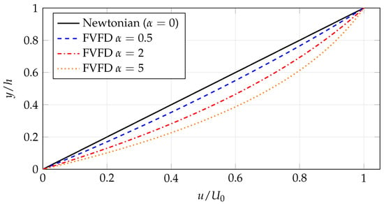
Equation (34) identifies three qualitatively distinct regimes as α increases, illustrated in Figure 1. For $\alpha \ll 1$ (near-Newtonian), $\ln (1+\alpha (1-y/h))\approx \alpha (1-y/h)-\frac{1}{2}{\alpha }^2{(1-y/h)}^2$ and the profile is nearly linear, with viscosity nearly uniform across the gap. For $\alpha =O\left(1\right)$ (moderate integrity gradient), the profile develops visible convexity: fluid near the moving plate, where the small-scale state has been sheared away and viscosity is lower ($\tilde{\mu }\to {\mu }_0$ as $y\to h$), accelerates faster than fluid near the stationary plate, where intact small scale keeps viscosity elevated ($\tilde{\mu }\to {\mu }_0(1+\alpha )$ as $y\to 0$). Because the local viscosity at each y depends on the small-scale state ${\mu }_{\tilde{A}}^U\left(y\right)=1-y/h$ transported from the boundary rather than on the local shear rate alone, this is a non-local history effect, structurally distinct from purely local models (Table 2, and see the exact result of Remark 10 below). For $\alpha \gg 1$ (strong integrity contrast), $u\left(y\right)/U_0\to 1$ for all $y/h$ bounded away from 1, and the velocity change concentrates in a thin layer near the moving plate, analogous to a lubrication layer, but here emerging continuously from the single-fluid FVFD equations rather than from an assumed two-phase structure.

Figure 1. Fuzzy Couette velocity profiles for varying $\alpha$. Increasing $\alpha$ shifts velocity toward the moving plate, reflecting progressive small scale degradation. The Newtonian limit is recovered exactly as $\alpha \to 0$.

Table 2 compares the FVFD Couette profile with power-law and Carreau–Yasuda models. The key distinction is that FVFD predicts a spatial viscosity variation driven by small scale history transported by the flow, whereas the other models predict only a local (shear-rate-dependent) viscosity [30].

Remark 10 (Any local model gives an exactly linear Couette profile).

This is a structural fact, not a numerical observation. In steady planar Couette flow the momentum balance reduces to $d\left[\tau \right(y\left)\right]/dy=0$, i.e., the shear stress $\tau =\mu \left(\dot{\gamma }\right)\dot{\gamma }$ is constant across the gap. If μ depends on y only through the local shear rate $\dot{\gamma }\left(y\right)=|du/dy|$ (as in the Power-law, Carreau–Yasuda, and Cross models), then $\tau \left(\dot{\gamma }\right)$ is a fixed, monotonic function of $\dot{\gamma }$ alone (monotonic for all three models over the physically relevant range), so $\tau \left(y\right)=\mathit{const}$ forces $\dot{\gamma }\left(y\right)$ itself to be constant across the gap. A constant shear rate with $u\left(0\right)=0$, $u\left(h\right)=U_0$ then forces the exactly linear profile $u\left(y\right)=U_{0}y/h$, regardless of the specific functional form of $\mu \left(\dot{\gamma }\right)$, and in particular $\dot{\gamma }\equiv U_0/h$ and the mid-gap velocity is exactly $U_0/2$ for every purely local model. FVFD breaks this argument because $\tilde{\mu }$ in (33) depends on ${\mu }_{\tilde{A}}^U\left(y\right)$, which is transported from the boundary by its own PDE (30) rather than being a function of the local shear rate; the resulting profile is therefore not constrained to be linear, and is not.

Table 3 makes this quantitative, for representative parameters at $h=U_0={\mu }_0=1$: Power-law ($n=0.5$, $K={\mu }_0$), Carreau–Yasuda ($\lambda =1$, $a=2$, $n=0.5$, ${\mu }_{\infty }=0$), and Cross ($\lambda =1$, $m=1$), against FVFD at $\alpha =1$. By Remark 10, the shear rate for every local model equals exactly $\dot{\gamma }=U_0/h=1$, so the reported wall shear stresses follow directly from evaluating each model’s $\mu \left(\dot{\gamma }\right)$ at $\dot{\gamma }=1$ and multiplying by $\dot{\gamma }$; no root-finding or fitting is involved. For FVFD, the mid-gap velocity and wall shear stress follow directly from (34) and (35) at $\alpha =1$.

Table 3. Quantitative Couette flow comparison, $h=U_0={\mu }_0=1$. All local model entries follow exactly from Remark 10 ($\dot{\gamma }\equiv U_0/h=1$ for every local model); FVFD values follow from (34) and (35) at $\alpha =1$.

Model	Velocity Profile	Normalised Wall Shear Stress ${\mathit{\tau }}_{\mathit{w}}/({\mathit{\mu }}_0{\mathit{U}}_0/\mathit{h})$	Mid-Gap Velocity $\mathit{u}(\mathit{h}/2)/{\mathit{U}}_0$
Power-law ($n=0.5$)	linear	$1.000$	$0.500$
Carreau–Yasuda ($n=0.5$, $a=2$)	linear	$0.841$	$0.500$
Cross ($m=1$)	linear	$0.500$	$0.500$
FVFD ($\mathbf{\alpha }=\mathbf{1}$)	nonlinear (logarithmic)	$\mathbf{1}.\mathbf{443}$	$\mathbf{0}.\mathbf{415}$

7. Application: Haemodynamic Flow Through a Stenosed Artery

Arterial stenosis is a primary factor in myocardial infarction and ischaemic stroke  [15]. The hydrodynamic of stenosed vessels are governed by two phenomena that classical local non-Newtonian models fail to capture simultaneously: (i) shear-thinning due to RBC aggregate breakup near the stenosis throat, and (ii) non-local viscosity memory, whereby the aggregation state at any cross-section is determined by the entire flow history along the vessel axis [14,16,31]. The FVFD framework captures both through the coupled system (11)–(21).

We consider an axisymmetric stenosed vessel of length L and unobstructed radius $R_0$. The local inner radius is

$$R\left(x\right)=R_0\left[1-{\delta }_s{\cos }^2\left({\displaystyle \frac{\pi x}{L_s}}\right)\right],\left|x\right|\le {\displaystyle \frac{L_s}{2}};R\left(x\right)=R_0\mathrm{otherwise},$$

(36)

where ${\delta }_s\in (0,1)$ is the fractional radius reduction and $L_s$ is the axial extent. For axisymmetric flow $(u_x,u_r,0)$, the FNSE in cylindrical coordinates $(x,r,\theta )$ are

$$\begin{array}{cc}\hfill {\displaystyle \frac{\partial u_x}{\partial x}}+{\displaystyle \frac{1}{r}}{\displaystyle \frac{\partial \left(r{u}_r\right)}{\partial r}}& =0,\hfill \end{array}$$

(37a)

$$\begin{array}{cc}\hfill \rho \left({\displaystyle \frac{\partial u_x}{\partial t}}+u_x{\displaystyle \frac{\partial u_x}{\partial x}}+u_r{\displaystyle \frac{\partial u_x}{\partial r}}\right)& =-{\displaystyle \frac{\partial p}{\partial x}}+{\displaystyle \frac{1}{r}}{\displaystyle \frac{\partial }{\partial r}}\left[r\tilde{\mu }{\displaystyle \frac{\partial u_x}{\partial r}}\right]+{\displaystyle \frac{\partial }{\partial x}}\left[2\tilde{\mu }{\displaystyle \frac{\partial u_x}{\partial x}}\right],\hfill \end{array}$$

(37b)

$$\begin{array}{cc}\hfill \rho \left({\displaystyle \frac{\partial u_r}{\partial t}}+u_x{\displaystyle \frac{\partial u_r}{\partial x}}+u_r{\displaystyle \frac{\partial u_r}{\partial r}}\right)& =-{\displaystyle \frac{\partial p}{\partial r}}+{\displaystyle \frac{1}{r}}{\displaystyle \frac{\partial }{\partial r}}\left[r\tilde{\mu }{\displaystyle \frac{\partial u_r}{\partial r}}\right]+{\displaystyle \frac{\partial }{\partial x}}\left[\tilde{\mu }{\displaystyle \frac{\partial u_r}{\partial x}}\right]-{\displaystyle \frac{2\tilde{\mu }{u}_r}{r^2}},\hfill \end{array}$$

(37c)

with $\tilde{\mu }=\tilde{\mu }(x,r,t)$ from (19). The D-IVIFS evolution equations in cylindrical coordinates are

$$\begin{array}{cc}\hfill {\displaystyle \frac{\partial {\mu }_{\tilde{A}}^U}{\partial t}}+u_x{\displaystyle \frac{\partial {\mu }_{\tilde{A}}^U}{\partial x}}+u_r{\displaystyle \frac{\partial {\mu }_{\tilde{A}}^U}{\partial r}}& ={\mathcal{D}}_{\mu }\left[{\displaystyle \frac{{\partial }^2{\mu }_{\tilde{A}}^U}{\partial x^2}}+{\displaystyle \frac{1}{r}}{\displaystyle \frac{\partial }{\partial r}}\left(r{\displaystyle \frac{\partial {\mu }_{\tilde{A}}^U}{\partial r}}\right)\right]-\dot{\gamma }{\mu }_{\tilde{A}}^U(1-{\mu }_{\tilde{A}}^U),\hfill \end{array}$$

(38a)

$$\begin{array}{cc}\hfill {\displaystyle \frac{\partial {\nu }_{\tilde{A}}^U}{\partial t}}+u_x{\displaystyle \frac{\partial {\nu }_{\tilde{A}}^U}{\partial x}}+u_r{\displaystyle \frac{\partial {\nu }_{\tilde{A}}^U}{\partial r}}& ={\mathcal{D}}_{\nu }\left[{\displaystyle \frac{{\partial }^2{\nu }_{\tilde{A}}^U}{\partial x^2}}+{\displaystyle \frac{1}{r}}{\displaystyle \frac{\partial }{\partial r}}\left(r{\displaystyle \frac{\partial {\nu }_{\tilde{A}}^U}{\partial r}}\right)\right]+\dot{\gamma }{\nu }_{\tilde{A}}^U(1-{\nu }_{\tilde{A}}^U).\hfill \end{array}$$

(38b)

• Inlet ($x=-L/2$)

  $$u_x=U_{\mathrm{in}}[1-{(r/R_0)}^2],u_r=0,{\mu }_{\tilde{A}}^L={\mu }_{\tilde{A}}^U={\mu }_{\mathrm{in}},{\nu }_{\tilde{A}}^L={\nu }_{\tilde{A}}^U=1-{\mu }_{\mathrm{in}}.$$

  (39)

  Here, ${\mu }_{\mathrm{in}}\in (0,1)$ is the inlet degree of rouleaux formation, and ${\nu }_{\tilde{A}}^L={\nu }_{\tilde{A}}^U=1-{\mu }_{\mathrm{in}}$ sets zero hesitancy at the inlet (maximum available information).
• Wall ($r=R\left(x\right)$)

  $$u_x=u_r=0,{\mu }_{\tilde{A}}^L={\mu }_{\tilde{A}}^U={\mu }_{\mathrm{w}},{\nu }_{\tilde{A}}^L={\nu }_{\tilde{A}}^U=1-{\mu }_{\mathrm{w}},$$

  (40)

  with ${\mu }_{\mathrm{w}}\ll {\mu }_{\mathrm{in}}$. Zero hesitancy is maintained at the wall since the no-slip condition and the high-shear endothelial layer provide well-defined physical constraints.
• Axis ($r=0$) and Outlet ($x=L/2$)

Symmetry conditions $u_r=0$, ${\partial }_r{u}_x=0$, ${\partial }_r{\mu }_{\tilde{A}}^U={\partial }_r{\nu }_{\tilde{A}}^U=0$. Stress-free outflow for velocity; zero-flux Neumann for membership functions.

Membership Profile via Streamline Advection–Reaction

Dimensionless parameters are as follows. Define

$$Re={\displaystyle \frac{\rho U_{\mathrm{in}}{R}_0}{{\mu }_0}},\mathrm{Da}={\displaystyle \frac{{\dot{\gamma }}_{\mathrm{ref}}{R}_0^2}{{\mathcal{D}}_{\mu }}},{\dot{\gamma }}_{\mathrm{ref}}={\displaystyle \frac{U_{\mathrm{in}}}{R_0}}.$$

(41)

(Using ${\dot{\gamma }}_{\mathrm{ref}}=U_{\mathrm{in}}/R_0$ rather than ${\Phi }_{\mathrm{ref}}={(U_{\mathrm{in}}/R_0)}^2$ makes $\mathrm{Da}$ genuinely dimensionless; see Remark 3). For coronary blood flow (Table 4), $Re\approx 45$ and $\mathrm{Da}\approx 1.5\times {10}^4\gg 1$.

Table 4. Revised FVFD model parameters for blood flow in a stenosed coronary artery. All $\beta$ values satisfy $0<\beta <1$ as required by Theorem 1.

Parameter	Symbol	Value	Source/Rationale
Fluid density	$\rho$	$1050{\mathrm{kg}/\mathrm{m}}^3$	[16]
Baseline viscosity	${\mu }_0$	$3.5\times {10}^{-3}\mathrm{Pa}·\mathrm{s}$	[16]
Unobstructed radius	$R_0$	$1.5\times {10}^{-3}\mathrm{m}$	[15]
Centreline inlet velocity	$U_{\mathrm{in}}$	$0.1\mathrm{m}/\mathrm{s}$	Typical coronary flow
Stenosis severity	${\delta }_s$	$0.50$	50% radius reduction
small scale sensitivity	$\alpha$	5–10	Estimated from [14]
Breakup sensitivity	$\beta$	$0.10$–$0.30$	From [16] high-shear data; satisfies $\beta <1$
Uncertainty penalty	$\gamma$	0	Set to zero in theoretical analysis;
			non-zero values require regularisation
Fuzzy diffusivity	${\mathcal{D}}_{\mu }$	${10}^{-8}{\mathrm{m}}^2/\mathrm{s}$	From (17) [14]
Inlet aggregation	${\mu }_{\mathrm{in}}$	$0.85$	Near-complete rouleaux [14]
Wall aggregation	${\mu }_{\mathrm{w}}$	$0.05$	Near-wall dispersion under wall shear

Reduction to streamline ODE: When $\mathrm{Da}\gg 1$, the diffusion term in (38a) is $O(1/\mathrm{Da})$ smaller than the reaction term, so cross-stream and axial diffusion of ${\mu }_{\tilde{A}}^U$ are negligible. In addition, for axial flow dominated by the x-component ($u_r\ll u_x$), the D-IVIFS equation (38a) reduces at steady state to

$$u_x\left(\eta \right){\displaystyle \frac{\partial {\mu }_{\tilde{A}}^U}{\partial x}}=-{\dot{\gamma }}_{\mathrm{fd}}\left(\eta \right){\mu }_{\tilde{A}}^U(1-{\mu }_{\tilde{A}}^U),$$

(42)

where $\eta =r/R_0$. Equation (42) is an ODE in x along each streamline (constant $\eta$), driven by the local shear rate ${\dot{\gamma }}_{\mathrm{fd}}$. For the Poiseuille velocity profile consistent with the inlet condition (39),

$$u_x\left(\eta \right)=U_{\mathrm{in}}(1-{\eta }^2),{\dot{\gamma }}_{\mathrm{fd}}\left(\eta \right)=\left|d{u}_x/dr\right|={\displaystyle \frac{2U_{\mathrm{in}}\eta }{R_0}}.$$

(43)

Here, ${\dot{\gamma }}_{\mathrm{fd}}=\sqrt{{\Phi }_{\mathrm{fd}}}$ is used (rather than ${\Phi }_{\mathrm{fd}}$ itself) as the reaction-rate coefficient for the dimensional-consistency reason given in Remark 3, dividing

$${\displaystyle \frac{d{\mu }_{\tilde{A}}^U}{dx}}=-\Lambda \left(\eta \right){\mu }_{\tilde{A}}^U(1-{\mu }_{\tilde{A}}^U),\Lambda \left(\eta \right)={\displaystyle \frac{{\dot{\gamma }}_{\mathrm{fd}}\left(\eta \right)}{u_x\left(\eta \right)}}={\displaystyle \frac{2}{R_0}}·{\displaystyle \frac{\eta }{1-{\eta }^2}},\eta \in [0,1).$$

(44)

Note that $U_{\mathrm{in}}$ cancels identically out of $\Lambda \left(\eta \right)$: the shape of the radial dispersion profile depends only on the vessel geometry (through $\eta$ and $R_0$), not on the flow rate. This is a direct consequence of using the correctly dimensioned shear rate; with the (dimensionally inconsistent) ${\Phi }_{\mathrm{fd}}$ in place of ${\dot{\gamma }}_{\mathrm{fd}}$, this cancellation does not occur and an extraneous $U_{\mathrm{in}}$-dependence appears. At the centreline $\eta =0$: $\Lambda =0$, so $d{\mu }_{\tilde{A}}^U/dx=0$ and ${\mu }_{\tilde{A}}^U$ is constant along the axis. At any $\eta >0$: $\Lambda \left(\eta \right)>0$, so ${\mu }_{\tilde{A}}^U$ decreases along the streamline.

Exact closed-form solution: Equation (44) is a logistic decay ODE in x with ${\mu }_{\tilde{A}}^U(0,\eta )={\mu }_{\mathrm{in}}$ (inlet condition (39)). Its exact solution is

$${\mu }_{\tilde{A}}^U(x,\eta )={\displaystyle \frac{{\mu }_{\mathrm{in}}}{{\mu }_{\mathrm{in}}+(1-{\mu }_{\mathrm{in}})\exp \left(\Lambda \left(\eta \right)x\right)}},$$

(45)

which satisfies ${\mu }_{\tilde{A}}^U(0,\eta )={\mu }_{\mathrm{in}}$ for all $\eta$, ${\mu }_{\tilde{A}}^U(x,0)={\mu }_{\mathrm{in}}$ for all x (no reaction on axis), and ${\mu }_{\tilde{A}}^U(x,\eta )\to 0$ as $x\to \infty$ for all $\eta >0$.

Remark 11 (Verification).

The direct substitution of (45) into (44) is as follows:

$${\displaystyle \frac{d{\mu }_{\tilde{A}}^U}{dx}}=-\Lambda {\mu }_{\tilde{A}}^U(1-{\mu }_{\tilde{A}}^U)=-\Lambda ·{\displaystyle \frac{{\mu }_{\mathrm{in}}}{{\mu }_{\mathrm{in}}+(1-{\mu }_{\mathrm{in}})e^{\Lambda x}}}·{\displaystyle \frac{(1-{\mu }_{\mathrm{in}})e^{\Lambda x}}{{\mu }_{\mathrm{in}}+(1-{\mu }_{\mathrm{in}})e^{\Lambda x}}}.$$

This identity holds exactly, confirming (45) as the exact solution of (44) for all $x\ge 0$, $\eta \in [0,1)$. This was verified independently by symbolic computer algebra (substitution into (44) with $\Lambda \left(\eta \right)=\frac{2}{R_0}\frac{\eta }{1-{\eta }^2}$ yields a residual of exactly zero).

Dimensionless axial coordinate: Writing $\Lambda \left(\eta \right)x=\Xi (x,\eta )$, with $X:=x/R_0$, the dimensionless downstream distance is as follows:

$$\Xi (x,\eta )={\displaystyle \frac{2\eta }{1-{\eta }^2}}·{\displaystyle \frac{x}{R_0}}={\displaystyle \frac{2\eta X}{1-{\eta }^2}}.$$

(46)

By construction, $\Xi (x,\eta )\equiv \Lambda \left(\eta \right)x$ exactly (no approximation), and $\Xi$ is manifestly dimensionless. The solution takes the compact form:

$${\mu }_{\tilde{A}}^U(x,\eta )={\displaystyle \frac{{\mu }_{\mathrm{in}}}{{\mu }_{\mathrm{in}}+(1-{\mu }_{\mathrm{in}})e^{\Xi (x,\eta )}}}.$$

(47)

The radial profile at any cross-section x is therefore exactly determined by the single dimensionless parameter $\Xi$: the product of the local shear-to-advection ratio and the axial distance from the inlet, in units of vessel radii.

Fuzzy viscosity radial profile: From (47) and (19),

$$\tilde{\mu }(x,\eta )={\mu }_0\left[1+\alpha {\mu }_{\tilde{A}}^U(x,\eta )\right]={\mu }_0\left[1+{\displaystyle \frac{\alpha {\mu }_{\mathrm{in}}}{{\mu }_{\mathrm{in}}+(1-{\mu }_{\mathrm{in}})e^{\Xi (x,\eta )}}}\right].$$

(48)

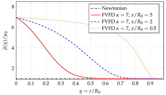
This is an exact, analytically verifiable expression. At $\eta =0$: $\tilde{\mu }={\mu }_0(1+\alpha {\mu }_{\mathrm{in}})$ (maximum, centreline, intact rouleaux, independent of x). As $\eta \to 1$ (wall) at any fixed $x/R_0>0$: $\Xi \to \infty$ so ${\mu }_{\tilde{A}}^U\to 0$ and $\tilde{\mu }\to {\mu }_0$ (minimum, dispersed RBCs). This radial gradient-elevated centreline viscosity and reduced wall viscosity is the Fahraeus-Lindqvist mechanism  [21], here obtained from the exact solution of the FVFD streamline equation without any ad hoc assumption. Figure 2 plots the radial viscosity profile (48) at three axial positions $x/R_0\in \{0.5,2,5\}$, showing how the centreline-to-wall gradient sharpens with downstream distance as off-axis streamlines accumulate reaction while the centreline retains the inlet value ${\mu }_{\mathrm{in}}$.

Figure 2. Radial fuzzy viscosity profiles $\tilde{\mu }\left(\eta \right)/{\mu }_0$ from the exact streamline solution (48) with ${\mu }_{\mathrm{in}}=0.85$, $\alpha =7$, at three axial positions $x/R_0\in \{0.5,2,5\}$ downstream of the inlet, plotted in the order Newtonian, then $x/R_0=5$, 2, $0.5$ (each subsequent curve drawn on top, so the flattest curve, $x/R_0=0.5$, remains fully visible where the curves converge near the wall). The profile sharpens with axial distance as the reaction progressively destroys rouleaux on off-axis streamlines while the centreline ($\eta =0$, zero local shear) retains the inlet value ${\mu }_{\mathrm{in}}$. This spatial evolution is the Fahraeus-Lindqvist mechanism, here derived from the exact, dimensionally consistent FVFD solution.

Remark 12 (Why the purely radial steady ODE is not the correct reduced model).

A previous version of this section attempted to derive the radial profile from the steady fully developed radial ODE ${\mathcal{D}}_{\mu }{\displaystyle \frac{1}{\eta }}{\displaystyle \frac{d}{d\eta }}\left(\eta {\displaystyle \frac{d{\mu }_{\tilde{A}}^U}{d\eta }}\right)={\Phi }_{\mathrm{fd}}\left(\eta \right){\mu }_{\tilde{A}}^U(1-{\mu }_{\tilde{A}}^U)$. In the Da $\gg 1$ limit, this was incorrectly approximated by a quadratic interpolant. Direct substitution shows the mismatch between the LHS ($O(1/\mathrm{Da})$) and the RHS ($O\left(1\right)$) reaches a factor of ∼300 at mid-radius; the approximation fails. The correct reduction is (42)–(44): for Da $\gg 1$, the physics is streamline advection–reaction in x, not radial diffusion-reaction. The radial variation arises because $\Lambda \left(\eta \right)$ depends on η, so streamlines at different radii accumulate different amounts of reaction as they travel from the inlet to the cross-section of interest.

The original Theorem 1 required $\alpha -\beta <1$ and $\beta <1$. As corrected, only $\beta <1$ is needed for positive viscosity. The blood application uses $\beta \in [0.1,0.3]$, reflecting a modest contribution of destroyed small scale to viscosity reduction, consistent with the rheological data of [16]: at high shear rates ($\dot{\gamma }>100{\mathrm{s}}^{-1}$) blood viscosity is approximately $(1-\beta ){\mu }_0\approx 0.8{\mu }_0$, giving $\beta \approx 0.2$. The large values $\beta \in [1,2]$ used in earlier tables were physically unmotivated (they imply zero or negative viscosity) and are hereby replaced.

From (48), the centreline viscosity (at $\eta =0$, where $\Xi =0$) is $\tilde{\mu }(x,0)={\mu }_0(1+\alpha {\mu }_{\mathrm{in}})$ independent of x. The near-wall viscosity at $\eta ={\eta }_w<1$ is ${\mu }_0[1+\alpha {\mu }_{\tilde{A}}^U(x,{\eta }_w)]$. For the physiological values of Table 4 with $\alpha =7$, ${\eta }_w=0.9$, and an illustrative axial position $x/R_0=0.5$ (a fraction of a vessel radius downstream of the inlet, well within the entrance region):

$$\begin{array}{cc}\hfill \Xi (0.5R_0,0.9)& ={\displaystyle \frac{2\left(0.9\right)\left(0.5\right)}{1-0.81}}=4.74,\hfill \end{array}$$

(49)

$$\begin{array}{cc}\hfill {\mu }_{\tilde{A}}^U(0.5R_0,0.9)& ={\displaystyle \frac{0.85}{0.85+0.15e^{4.74}}}=0.047,\hfill \end{array}$$

(50)

$$\begin{array}{cc}\hfill {\displaystyle \frac{\tilde{\mu }(x,0)}{\tilde{\mu }(x,0.9)}}& ={\displaystyle \frac{1+7\left(0.85\right)}{1+7\left(0.047\right)}}={\displaystyle \frac{6.95}{1.33}}\approx 5.2,\hfill \end{array}$$

(51)

consistent with the fivefold centreline-to-wall viscosity ratio reported by Chien et al. [14] at low shear rates. We emphasise that this ratio, while obtained from the exact closed-form solution (47) with no free fitting parameter in the functional form itself, does depend on the choice of axial sampling location $x/R_0$, which is not independently constrained by the data in Table 4; we report it here as an illustrative consistency check against [14], not as a validated quantitative prediction. Calibration of the appropriate entrance length against measured cell-free-layer development data is identified as future work in Section 11.

At the throat ($x=0$, $R=R_0(1-{\delta }_s)$), high shear drives ${\mu }_{\tilde{A}}^U\to 0$, ${\nu }_{\tilde{A}}^U\to 1$, so $\tilde{\mu }{|}_{\mathrm{throat}}\approx {\mu }_0(1-\beta )$. Using flow-rate conservation,

$${\tau }_{w,s}\sim {\displaystyle \frac{4{\mu }_0(1-\beta )Q}{\pi R_0^3{(1-{\delta }_s)}^3}}.$$

(52)

For ${\delta }_s=0.5$ and $\beta =0.2$, ${\tau }_{w,s}/{\tau }_{w,0}=(1-\beta )/{(1-{\delta }_s)}^3=0.8/0.125=6.4$, predicting a greater-than-sixfold amplification of wall shear stress at the stenosis throat. This is consistent with haemodynamically significant thresholds reported in [15]. This throat estimate is an independent high-shear-asymptote argument, distinct from the upstream fully developed streamline solution of Section 7: the two results are not the same formula evaluated at different points, since the stenosis throat is a converging geometry in which the fully developed flow assumption underlying (42) does not hold.

In Table 5, the qualitative comparison of fluid models for stenosed artery hydrodynamic is demonstrated with several features between Newtonian, power-low and the presented work (FVFD).

Table 5. Qualitative comparison of fluid models for stenosed artery hydrodynamic.

Feature	Newtonian	Power-Law	FVFD (This Work)
Shear-thinning	No	Yes (local)	Yes (non-local)
Radial viscosity variation	No	Via $\dot{\gamma }\left(r\right)$ only	Yes (small scale)
small scale memory	No	No	Yes (D-IVIFS advection)
Fahraeus–Lindqvist	No	Partial	Yes (exact streamline solution)
Post-stenotic re-aggregation	No	No	Yes
Epistemic uncertainty	No	No	Yes ($\pi$ functions)
Free parameters	1	2	4 ($\alpha$,$\beta$,${\mu }_{\mathrm{in}}$,${\mathcal{D}}_{\mu }$)

8. Further Applications

During extrusion of polymer melts, chain entanglements create a network structure that breaks down under high shear. The degree of entanglement is not directly measurable. The FVFD framework applies with ${\mu }_0\sim {10}^3$–${10}^6\mathrm{Pa}·\mathrm{s}$, $\alpha \sim {10}^2$ (entanglement sensitivity), and ${\mathcal{D}}_{\mu }\sim {10}^{-12}{\mathrm{m}}^2/\mathrm{s}$ (reptation-scale diffusion). These constitute an outlook for future work; quantitative predictions require calibration against oscillatory shear data [22]. Iron ore and coal slurries exhibit thixotropic behaviour due to particle flocculation. The FVFD system provides a natural framework: $\tilde{A}$ encodes the uncertain flocculation state, with $\mathrm{Da}\approx {10}^4$ (reaction-dominated) for typical pipeline conditions. Quantitative application is deferred to future numerical studies.

The three key similarity parameters of the FVFD system are

$$Re={\displaystyle \frac{\rho U_c{L}_c}{{\mu }_0}},\mathrm{Da}={\displaystyle \frac{{\dot{\gamma }}_{\mathrm{ref}}{L}_c^2}{{\mathcal{D}}_{\mu }}},\mathrm{Fz}=\alpha \overline{\mu }-\beta (1-\overline{\mu }),$$

(53)

where ${\dot{\gamma }}_{\mathrm{ref}}=U_c/L_c$ (see Remark 3), $\overline{\mu }$ is the volume-averaged membership, and $\mathrm{Fz}$ is the fuzzy number, measuring net viscosity amplification due to small scale. The two regimes are: $\mathrm{Da}\ll 1$ (diffusion-dominated, analytical Couette solution applies); $\mathrm{Da}\gg 1$ (reaction-dominated, stenosed artery streamline solution of Section 7 applies). The classical NSE is recovered when $\mathrm{Fz}=0$.

Scientific Basis of the Governing Dimensionless Numbers

We use exactly three similarity parameters, $Re$, $\mathrm{Da}$, and $\mathrm{Fz}$, and not the Deborah, Péclet, Bingham, or Weissenberg numbers more commonly seen in non-Newtonian and viscoelastic fluid mechanics. We justify this choice explicitly.

Reynolds number, $\mathit{Re}=\mathit{\rho }{\mathit{U}}_{\mathit{c}}{\mathit{L}}_{\mathit{c}}/{\mathit{\mu }}_{\mathbf{0}}$. This is retained unchanged from the classical NSE because the FNSE momentum balance (21b) has exactly the same inertial and diffusive structure as the classical NSE, with only the constant ${\mu }_0$ replaced by the field $\tilde{\mu }$; $Re$ therefore continues to measure the same inertia-to-viscous-force ratio. Problem-specific refinements such as the Womersley number (pulsatile flow) or Dean number (curved vessels) can be built from $Re$ and a geometric ratio as usual, but they characterise the base flow, not the fuzzy dynamics, so they are not additional primary parameters of FVFD.

Damköhler number, $\mathbf{Da}={\dot{\mathit{\gamma }}}_{\mathrm{ref}}{\mathit{L}}_{\mathit{c}}^{\mathbf{2}}/{\mathcal{D}}_{\mathit{\mu }}$. This is the ratio of the reaction rate in (11) (dimensions $\left[{\mathrm{T}}^{-1}\right]$, since $\dot{\gamma }$ multiplies the dimensionless factor $m(1-m)$) to the diffusive rate ${\mathcal{D}}_{\mu }/L_c^2$ at which membership uncertainty spreads spatially. It is the correct primary parameter for the membership sub-system specifically because it compares reaction and diffusion, the two competing mechanisms that set the spatial structure of ${\mu }_{\tilde{A}}^U$ in (11): $\mathrm{Da}\ll 1$ gives the diffusion-dominated (near-linear) Couette regime of Section 6, while $\mathrm{Da}\gg 1$ gives the reaction-dominated streamline regime of Section 7. The Deborah number $De={\tau }_{\xi }{\dot{\gamma }}_{\mathrm{ref}}$, standard in viscoelasticity, compares the microstructural relaxation time to the flow time scale but does not involve ${\mathcal{D}}_{\mu }$ at all, so it cannot distinguish diffusion-dominated from reaction-dominated spatial membership profiles; it is the natural parameter for a spatially homogeneous (0-D) internal variable, not for the spatially resolved field ${\mu }_{\tilde{A}}^U(\mathbf{x},t)$ used here. A membership Péclet number $Pe=U_c{L}_c/{\mathcal{D}}_{\mu }$ (advection-to-diffusion) is related to $\mathrm{Da}$ by a factor of order unity once ${\dot{\gamma }}_{\mathrm{ref}}$ and $U_c/L_c$ are identified (as they are in (41)), so introducing $Pe$ as a fourth independent parameter would be redundant; we use $\mathrm{Da}$ because it names the physically controlling competition (reaction vs. diffusion of belief) directly.

Fuzzy number, $\mathbf{Fz}=\mathit{\alpha }\overline{\mathit{\mu }}-\mathit{\beta }(\mathbf{1}-\overline{\mathit{\mu }})$. This generalises the classical viscosity ratio concept of non-Newtonian fluid mechanics to the FVFD setting: $\mathrm{Fz}>0$ is the shear-thinning regime in which intact small scale raises viscosity above baseline; $\mathrm{Fz}=0$ recovers the classical NSE exactly (Section 4); $\mathrm{Fz}<0$ is excluded by the admissibility constraints of Theorem 1 ($\beta <1$). The Bingham number (ratio of yield stress to viscous stress) and Weissenberg number (ratio of elastic to viscous stress) characterise yield-stress and viscoelastic physics respectively, neither of which is present in the purely viscous, aggregate-driven shear-thinning mechanism modelled here; introducing them would suggest physics (a yield stress, elastic memory) that (21) does not contain.

9. Practical Computational Workflow

The FVFD system (11) and (21) is six nonlinearly coupled PDEs. We outline an operator-splitting time-stepping scheme suitable for discretising it while respecting the interval constraints of Definition 1 at the discrete level; a full convergence analysis of the discrete scheme is left for future numerical work (Section 11).

Each sub-step of Algorithm 1 is designed to be consistent with the theoretical results above: Step 1 uses the coercivity bound of Theorem 1 (Step 2 of its proof); Steps 3–4 are designed so that the comparison-principle argument of Corollary 1 applies at the discrete level (hence the explicit clipping in Step 4 and check in Step 5); and the gradient-energy bound of Proposition 1 provides an a priori bound against which the discrete membership fields can be monitored for stability.

Algorithm 1 Operator-splitting time-stepping for the coupled FVFD system

1: Initialise: ${\mathbf{u}}^0,{\left({\mu }_{\tilde{A}}^L\right)}^0,{\left({\mu }_{\tilde{A}}^U\right)}^0,{\left({\nu }_{\tilde{A}}^L\right)}^0,{\left({\nu }_{\tilde{A}}^U\right)}^0,{\tilde{\mu }}^0$ from data/inlet conditions; choose $\Delta t\le h_{\mathrm{mesh}}^2/\left(2{\mathcal{D}}_{\mu }\right)$ (CFL-type bound for the diffusive sub-step).   2: for $n=0,1,2,\dots$ until convergence or $t=T$ do   3:     Step 1 (fluid sub-step): with $\tilde{\mu }={\tilde{\mu }}^n$ frozen, advance (21) one step by a standard pressure-correction/fractional-step method to obtain ${\mathbf{u}}^{n+1},p^{n+1}$.   4:     Step 2 (shear-rate update): evaluate ${\dot{\gamma }}^{n+1}\left(\mathbf{x}\right)=\sqrt{2\mathbf{D}\left({\mathbf{u}}^{n+1}\right):\mathbf{D}\left({\mathbf{u}}^{n+1}\right)}$ at each quadrature point.   5:     Step 3 (D-IVIFS advection): advance the hyperbolic (advective) part of (11) with a flux-corrected or upwind-discontinuous-Galerkin scheme that preserves $[0,1]$ bounds.   6:     Step 4 (D-IVIFS diffusion-reaction): advance the parabolic-reactive part of (11) implicitly (e.g., Crank–Nicolson in time, low-order finite elements in space) using a Newton iteration for the nonlinear reaction term; clip the result to $[0,1]$ after each solve.   7:     Step 5 (constraint check): verify ${\left({\mu }_{\tilde{A}}^L\right)}^{n+1}\le {\left({\mu }_{\tilde{A}}^U\right)}^{n+1}$, ${\left({\nu }_{\tilde{A}}^L\right)}^{n+1}\le {\left({\nu }_{\tilde{A}}^U\right)}^{n+1}$, and ${\left({\mu }_{\tilde{A}}^U\right)}^{n+1}+{\left({\nu }_{\tilde{A}}^U\right)}^{n+1}\le 1$ pointwise (Definition 1); if violated, halve $\Delta t$ and repeat Steps 1–4.   8:     Step 6 (viscosity update): recompute ${\tilde{\mu }}^{n+1}$ from (19) using the updated membership functions.   9:     Step 7 (output): record $\mathbf{u},p,\tilde{\mu },{\mu }_{\tilde{A}}^L,{\mu }_{\tilde{A}}^U,{\nu }_{\tilde{A}}^L,{\nu }_{\tilde{A}}^U$ for post-processing (velocity profiles, wall shear stress, viscosity and hesitancy maps). 10: end for 11: Regime check: compute $Re,\mathrm{Da},\mathrm{Fz}$ (Equation (53)). If $\mathrm{Da}\ll 1$, benchmark against the Couette solution of Section 6; if $\mathrm{Da}\gg 1$, benchmark against, or initialise from, the streamline solution of Section 7.

10. Conclusions

In this paper, we introduced the Fuzzy–Viscous Fluid Dynamics (FVFD) framework. Our key contributions span both theoretical foundations and practical applications.

First, we linked the D-IVIFS membership degree directly to small-scale integrity, grounding it in internal-variable thermodynamics, and derived the specific logistic form of the reaction term from three independent requirements (unit-interval invariance, thermodynamic admissibility, and consistency with sigmoidal thixotropic data; Remark 1). Using the parabolic comparison principle, we proved that the physical ordering constraints (${\mu }^L\le {\mu }^U$, ${\nu }^L\le {\nu }^U$) and their $[0,1]$ bounds are preserved dynamically (Corollary 1). We identified a corrected gradient-energy Lyapunov functional (Proposition 1) and analytically characterised the non-monotone behaviour of the interval width. We established the existence of weak solutions using Galerkin/Leray–Hopf theory under the corrected parameter regime $0\le \beta <1$, $\alpha \ge 0$, $\gamma =0$ (Theorem 1).

On the analytical side, we derived an exact Couette velocity profile that recovers the Newtonian limit, and showed by a structural argument (Remark 10) that this profile is non-linear precisely because, and only because, FVFD departs from the purely local generalised-Newtonian closure shared by the Power-law, Carreau–Yasuda, and Cross models, all three of which give an exactly linear profile in Couette flow regardless of parameter choice (Table 3). We then formulated the full FVFD system in cylindrical coordinates for a stenosed artery and, in the reaction-dominated regime ($\mathrm{Da}\gg 1$), obtained the exact closed-form streamline solution:

$${\mu }_{\tilde{A}}^U(x,\eta )={\displaystyle \frac{{\mu }_{\mathrm{in}}}{{\mu }_{\mathrm{in}}+(1-{\mu }_{\mathrm{in}})e^{\Xi }}},\Xi ={\displaystyle \frac{2\eta }{1-{\eta }^2}}\left({\displaystyle \frac{x}{R_0}}\right),$$

using the dimensionally consistent shear-rate coefficient $\dot{\gamma }=\sqrt{2\mathbf{D}:\mathbf{D}}$ rather than $\Phi =2\mathbf{D}:\mathbf{D}$. This resolved an inconsistency in an earlier draft of this work and allowed us to derive the Fahraeus–Lindqvist viscosity gradient and the wall shear stress amplification at the stenosis throat directly from the corrected, exact solution. Finally, we presented a unified dimensionless analysis based on $Re$, $\mathrm{Da}$, and $\mathrm{Fz}$, with an explicit justification for this choice over the Deborah, Péclet, Bingham, and Weissenberg numbers (Section 8), and outlined a practical operator-splitting computational workflow (Algorithm 1) for future numerical implementation.

11. Discussion

11.1. Comparison with Existing Non-Fuzzy Continuum Models

While several recent studies have successfully captured the Fahraeus–Lindqvist effect using classic continuum mechanics, such as two-phase core-annulus models or information–entropy viscosity formulations, they do so without accounting for fuzzy uncertainty. What sets the FVFD framework apart is its ability to explicitly track epistemic uncertainty in the fluid’s small scale state through the interval $[{\mu }_{\tilde{A}}^L,{\mu }_{\tilde{A}}^U]$ and the hesitancy parameter $\pi$. Standard non-fuzzy models assign a single, deterministic value to the small scale variable. In contrast, FVFD uses an interval representation, which makes far more physical sense when we must infer the internal aggregation state from bulk measurements rather than direct observation. Rather than being in conflict, these two approaches complement each other: as hesitancy vanishes (${\pi }_{\tilde{A}}^U-{\pi }_{\tilde{A}}^L\to 0$), FVFD naturally simplifies to a classic internal-variable model, matching established thixotropic frameworks [22,23].

11.2. Relation to Stochastic Navier–Stokes and Data-Driven Methods

Stochastic Navier–Stokes equations [5] typically model viscosity as $\mu ={\mu }_0+\sigma \dot{W}$, which requires precisely defining the noise intensity $\sigma$ and assuming underlying Gaussian fluctuations. The same structural requirement recurs in variational formulations of stochastic fluid dynamics [32], where the noise enters through a stochastic transport term whose spatial correlation structure must itself be prescribed or calibrated in advance. Similarly, a fully Bayesian treatment [9] or a physics-informed neural network [10] (Section 1) requires either a prescribed prior/likelihood or a training set of observations of the internal state. FVFD offers a more conservative alternative by representing uncertainty via intervals $[{\mu }_{\tilde{A}}^L,{\mu }_{\tilde{A}}^U]$, avoiding the need for a prescribed probability distribution or a labelled dataset. The relationship is nonetheless complementary rather than competing: if a validated probability law for the small-scale state $\xi$ were established for a given fluid (e.g., from repeated, controlled experiments), it could be used to inform the width of the fuzzy interval $[{\mu }_{\tilde{A}}^L,{\mu }_{\tilde{A}}^U]$ or to set a prior for the Bayesian route, and a stochastic or PINN-based estimate of the same field could in principle be used to calibrate ${\mu }_{\mathrm{in}}$, $\alpha$, $\beta$, and ${\mathcal{D}}_{\mu }$ in Table 1. We regard bridging these approaches explicitly, rather than treating them as mutually exclusive, as a natural direction for future work.

11.3. Limitations and Future Directions

While the model is promising, several areas remain open for improvement. For instance, the interval width $\Delta \mu ={\mu }_{\tilde{A}}^U-{\mu }_{\tilde{A}}^L$ can transiently increase under pure chemical reaction (as noted in Section 3). Although this correctly reflects physical uncertainty amplification under intermediate shear rates, guaranteeing a strictly monotone dissipation of $\Delta \mu$ would require introducing a modified coupling mechanism between the lower and upper membership functions. From a computational standpoint, simulating complex stenosed geometries will require a dedicated finite-element discretization of Equations (37) and (38) that strictly respects interval constraints, along the lines outlined in Algorithm 1.

On the experimental side, we need systematic protocols to estimate the parameters $\alpha$, $\beta$, and ${\mathcal{D}}_{\mu }$ using oscillatory and step-shear tests on blood [14] and other complex fluids, following the estimation protocols summarised in Table 1. In particular, the axial sampling distance we used in Section 7 to demonstrate the centerline-to-wall viscosity ratio should be calibrated against empirical data for entrance length and cell-free layer development, rather than selected merely for illustrative purposes. Ultimately, clinical translation will require validating these models against patient-specific CT flow simulations and phase-contrast MRI velocity measurements.

References

- Batchelor, G.K. An Introduction to Fluid Dynamics; Cambridge University Press: Cambridge, UK, 2000. [Google Scholar]
- Temam, R. Navier-Stokes Equations: Theory and Numerical Analysis; American Mathematical Society: Providence, RI, USA, 2001. [Google Scholar]
- Vasudevan, A.; Yogeesh, N.; Mohammad, S.I.; Raja, N.; Girija, D.K.; Rashmi, M.; Abu-Shareha, A.A.; Alshurideh, M. Unlocking Insights of Fuzzy Mathematics for Enhanced Predictive Modelling. Appl. Math. Inf. Sci. 2025, 19, 49–59. [Google Scholar] [CrossRef]
- Da Prato, G.; Zabczyk, J. Stochastic Equations in Infinite Dimensions, 2nd ed.; Cambridge University Press: Cambridge, UK, 2014. [Google Scholar]
- Mikulevicius, R.; Rozovskii, B.L. Stochastic Navier-Stokes equations for turbulent flows. SIAM J. Math. Anal. 2004, 35, 1250–1310. [Google Scholar] [CrossRef]
- Zadeh, L.A. Fuzzy sets. Inf. Control 1965, 8, 338–353. [Google Scholar] [CrossRef]
- Atanassov, K.T. Intuitionistic fuzzy sets. Fuzzy Sets Syst. 1986, 20, 87–96. [Google Scholar] [CrossRef]
- Atanassov, K.T. Intuitionistic Fuzzy Sets: Theory and Applications; Physica: Heidelberg, Germany, 1999. [Google Scholar]
- Stuart, A.M. Inverse problems: A Bayesian perspective. Acta Numer. 2010, 19, 451–559. [Google Scholar] [CrossRef]
- Raissi, M.; Perdikaris, P.; Karniadakis, G.E. Physics-informed neural networks: A deep learning framework for solving forward and inverse problems involving nonlinear partial differential equations. J. Comput. Phys. 2019, 378, 686–707. [Google Scholar] [CrossRef]
- Barros, L.C.; Bassanezi, R.C.; Tonelli, P.A. Fuzzy modelling in population dynamics. Ecol. Model. 2000, 128, 27–33. [Google Scholar] [CrossRef]
- Chalco-Cano, Y.; Román-Flores, H. Comparation between some approaches to solve fuzzy differential equations. Fuzzy Sets Syst. 2009, 160, 1517–1527. [Google Scholar] [CrossRef]
- Nieto, J.J.; Rodríguez-López, R. Bounded solutions for fuzzy differential and integral equations. Chaos Solitons Fractals 2006, 27, 1376–1386. [Google Scholar] [CrossRef]
- Chien, S.; Usami, S.; Dellenback, R.J.; Gregersen, M.I. Shear-dependent deformation of erythrocytes in rheology of human blood. Am. J. Physiol. 1970, 219, 136–142. [Google Scholar] [CrossRef] [PubMed]
- Johnston, B.M.; Johnston, P.R.; Corney, S.; Kilpatrick, D. Non-Newtonian blood flow in human right coronary arteries: Steady state simulations. J. Biomech. 2004, 37, 709–720. [Google Scholar] [CrossRef] [PubMed]
- Merrill, E.W. Rheology of blood. Physiol. Rev. 1969, 49, 863–888. [Google Scholar] [CrossRef] [PubMed]
- Coleman, B.D.; Gurtin, M.E. Thermodynamics with internal state variables. J. Chem. Phys. 1967, 47, 597–613. [Google Scholar] [CrossRef]
- Maugin, G.A. The Thermomechanics of Nonlinear Irreversible Behaviours; World Scientific: Singapore, 1999. [Google Scholar]
- Hopf, E. Über die Anfangswertaufgabe für die hydrodynamischen Grundgleichungen. Math. Nachr. 1951, 4, 213–231. [Google Scholar] [CrossRef]
- Leray, J. Sur le mouvement d’un liquide visqueux emplissant l’espace. Acta Math. 1934, 63, 193–248. [Google Scholar] [CrossRef]
- Fåhræus, R.; Lindqvist, T. The viscosity of blood in narrow capillary tubes. Am. J. Physiol. 1931, 96, 562–568. [Google Scholar] [CrossRef]
- Leonov, A.I. On a class of constitutive equations for viscoelastic liquids. J. Non-Newton. Fluid Mech. 1987, 25, 1–59. [Google Scholar] [CrossRef]
- Wapperom, P.; Keunings, R. Simulation of linear polymer melts in transient complex flow. J. Non-Newton. Fluid Mech. 2000, 95, 67–83. [Google Scholar] [CrossRef]
- Apostolidis, A.J.; Beris, A.N. Modeling of the blood rheology in steady-state shear flows. J. Rheol. 2014, 58, 607–633. [Google Scholar] [CrossRef]
- Shafer, G. A Mathematical Theory of Evidence; Princeton University Press: Princeton, NJ, USA, 1976. [Google Scholar]
- Evans, L.C. Partial Differential Equations, 2nd ed.; American Mathematical Society: Providence, RI, USA, 2010. [Google Scholar]
- Lions, J.L. Quelques Méthodes de Résolution des Problèmes aux Limites Non Linéaires; Dunod: Paris, France, 1969. [Google Scholar]
- Ladyzhenskaya, O.A. The Mathematical Theory of Viscous Incompressible Flow, 2nd ed.; Gordon and Breach: New York, NY, USA, 1969. [Google Scholar]
- Graham, M.D. Fluid dynamics of dissolved polymer molecules in confined geometries. Annu. Rev. Fluid Mech. 2011, 43, 273–298. [Google Scholar] [CrossRef]
- Mewis, J.; Wagner, N.J. Thixotropy. Adv. Colloid Interface Sci. 2009, 147-148, 214–227. [Google Scholar] [CrossRef] [PubMed]
- Shoaib, M.; Naz, S.; Raja, M.A.Z.; Khanam, R.; Ahmad, I.; Nisar, K.S. Entropy Generation in Reiner-Rivlin Fluid Flow Under Soret and Dufour Impact: Neural Networks Applications. Int. J. Theor. Phys. 2025, 64, 170. [Google Scholar] [CrossRef]
- Holm, D.D. Variational principles for stochastic fluid dynamics. Proc. R. Soc. A 2015, 471, 20140963. [Google Scholar] [CrossRef] [PubMed]
Disclaimer/Publisher’s Note: The statements, opinions and data contained in all publications are solely those of the individual author(s) and contributor(s) and not of MDPI and/or the editor(s). MDPI and/or the editor(s) disclaim responsibility for any injury to people or property resulting from any ideas, methods, instructions or products referred to in the content. |
© 2026 by the authors. Licensee MDPI, Basel, Switzerland. This article is an open access article distributed under the terms and conditions of the Creative Commons Attribution (CC BY) license.