


Abstract
The k-nearest neighbor (KNN) algorithm remains one of the most fundamental and widely-used methods in machine learning. A common rule of thumb sets the number of neighbors as , where n is the size of the training set. Despite its widespread adoption, the theoretical justification for this choice has remained obscure. We provide a comprehensive rate-based analysis. First, we derive the minimax-optimal exponent for under standard Hölder-smoothness assumptions, recovering as a special case Theorem 1: under these second-order Hölder-smoothness assumptions, attains the asymptotic minimax-optimal exponent if and only if the feature space has dimensionality ; this concerns the asymptotic rate exponent, not the finite-sample optimal value of k. Second, Theorem 2 quantifies the sub-optimality of any fixed as with , yielding an asymmetric penalty for the classical rule when that we make precise in Corollary 1. The predicted rate is empirically verified across on controlled synthetic data. On 48 datasets from the OpenML-CC18 benchmark suite, the dimension-aware rule outperforms the classical rule in 32 of 48 head-to-head comparisons (paired Wilcoxon , mean accuracy gain percentage points), demonstrating that the theoretical improvement translates to a practical one. We further test the Hassanat distance metric against Euclidean across all KNN variants on the same 48 datasets, finding that Hassanat outperforms Euclidean in five of six configurations (paired Wilcoxon ), with the largest gains on unstandardized data. Cross-validation remains the strongest k-selection strategy when computationally feasible, and the theoretical results provide a principled non-cross-validated alternative.
Keywords:
k-nearest neighbors; optimal k selection; square-root-of-n rule; minimax convergence rate; sub-optimality rate; dimension-aware neighbor selection; bias–variance tradeoff; Hölder smoothness; Hassanat distance; nonparametric classification MSC:
62G08; 62H30; 68T10; 62G20
1. Introduction
The k-nearest neighbor (KNN) algorithm, developed by Fix and Hodges (1951) [1] and formalized by Cover and Hart (1967) [2], is still one of the most intuitive and widely used classification algorithms in machine learning and other applications in general [3]. This method is widely used in several disciplines, such as the Internet of Things [4], data mining [5], and recommendation systems [6], where it supports critical capabilities of modern intelligent systems. More broadly, contemporary machine-learning practice spans evolutionary feature selection for high-dimensional medical data [7], human-based metaheuristic optimizers [8], and trust-aware explainable frameworks for sensitive domains such as mental-health classification; the rate-based analysis of k-NN developed here complements this landscape by supplying theoretical guidance for one of its most widely used building blocks.
KNN is a non-parametric, instance-based (“lazy”) method for classification and regression [9,10,11]: it requires no explicit training pass and classifies a query point by majority vote among its k nearest neighbours in the training set, under a chosen distance metric such as Euclidean, Manhattan, Hassanat, or Minkowski. The single hyperparameter k governs the balance between noise sensitivity and over-smoothing. Despite this simplicity, KNN rests on a solid theoretical foundation and performs well empirically across many applications.
A fundamental challenge in KNN is the selection of the hyperparameter k [12], which directly influences the bias–variance trade-off. Small k values result in high variation and sensitivity to noise, but higher values add bias by including distant and perhaps irrelevant samples. In practice, a popular heuristic (rule of thumb) is , where n is the size of the training set. This rule is widely mentioned in tutorials, textbooks, and practical research, such as [13,14,15], among others, but its connection to theoretical ideas is not fully explained.
More importantly, the choice of k is typically made exclusively based on sample size, ignoring other vital factors such as data quality, noise level, and distance metric behavior. This constraint emphasizes the importance of flexible, data-driven k-selection methods.
A thorough review of the literature, however, reveals an unexpected gap: although the rule is frequently used, its theoretical foundation is rarely given or justified.
- The persistence of in 2024–2026.
The first author has himself contributed to the propagation of this rule in their earlier work [15]. Therefore, it is worth documenting how widely it, and the equally common default of , are still being applied in recent peer-reviewed studies. Our non-exhaustive survey of 2024–2026 applied work shows that the rule remains an active default practice across multiple domains; the following are just examples:
- Medical and health informatics. A 2025 application of KNN to the Pima Indians Diabetes dataset [16], explicitly used as its selection rule without providing any further theoretical justification. Al-Khamees et al. [17] motivate their dynamic-k proposal precisely by observing that “traditional k-NN relies on a static k-value, which may not provide optimal results across diverse datasets”—a gap the present paper addresses theoretically rather than empirically. Other recent work applies KNN to fruit classification and quality assessment with a fixed, empirically chosen k and no principled selection criterion [18].
- IoT and cybersecurity. The proliferation of adaptive KNN variants in this domain—Adaptive SAMKNN for zero-day attack detection [19] and the three-branch decision soft-increment KNN for network intrusion detection [20], both published in 2025—is itself indirect evidence of the same gap: each of these papers patches the static-k problem empirically, without explaining when or why the underlying static rule fails.
- Finance and credit risk. Çetin and Büyüklü [21] introduce a feature-importance-weighted KNN for sovereign credit rating, but retain a fixed k chosen empirically. Othman et al. [22] apply standard KNN to loan-default prediction with no theoretical k-selection argument.
The present paper supplies that framework: we show that under second-order Hölder smoothness, attains the asymptotic minimax-optimal exponent if and only if (Theorem 1), we quantify how the rule fails when via a sharp sub-optimality rate (Theorem 2 and Corollary 1), and we verify both the rate and the resulting practical improvement on a large benchmark.
- Position of this paper.
This work sits at the intersection of computational statistics and nonparametric classification theory. Our central object of study is the asymptotic excess risk of the k-NN classifier viewed as a function of the polynomial exponent governing k, and our main mathematical contribution (Theorem 2 and Corollary 1) is a sharp rate characterization of how deviation from the minimax-optimal exponent inflates the regret. We treat empirical benchmarking as verification of the theoretical predictions rather than the principal contribution, and we explicitly distinguish between what the theory establishes (minimax rates and sub-optimality bounds) and what cross-validation delivers in practice (a strict upper bound on accuracy that no fixed non-cross-validated rule can match in general).
This paper makes the following contributions:
- We derive the minimax-optimal rate from first principles and demonstrate that emerges as a special case when (Theorem 1).
- We establish a sharp rate of sub-optimality for any fixed polynomial exponent (Theorem 2), and characterize the asymmetric penalty that the classical rule incurs across dimensions (Corollary 1).
- We verify the predicted convergence rates empirically on synthetic data with controlled dimensionality and known regression function.
- Across 48 datasets from the OpenML-CC18 benchmark suite, we demonstrate that the dimension-aware rule outperforms the classical rule, with the improvement statistically significant under a paired Wilcoxon test ().
- We further demonstrate that the Hassanat distance metric outperforms Euclidean across all three k-selection strategies on the same 48 datasets, particularly on unstandardized data.
- We release a Python (version 3.11) toolkit implementing the dimension-aware rule, the Hassanat distance, and cross-validated k-selection.
2. Theoretical Foundations
2.1. Preliminaries and Notation
Consider a random pair , where represents a d-dimensional feature vector and denotes the corresponding class label. Suppose a training dataset consists of n independent and identically distributed samples drawn from the joint distribution of .
Given a query point x, the k-nearest neighbor (k-NN) classifier predicts its label according to the majority class among the k closest training samples in .
For the binary classification setting, define the regression function as . The Bayes classifier, which minimizes the classification error, is defined as if , and otherwise. The corresponding minimum achievable risk, known as the Bayes risk, is given by
Let denote the classification risk of the k-NN classifier trained on . The performance gap between the k-NN classifier and the Bayes optimal classifier is measured by the excess risk (or regret), defined as
2.2. Bias-Variance Decomposition
- Smoothness premise.
Throughout Section 2, including Theorems 1 and 2 and their corollaries, we assume that the regression function satisfies the -Hölder smoothness condition with , i.e., is twice continuously differentiable on its support with second-order partial derivatives uniformly bounded by . We further assume that X is supported on a compact set with density bounded away from zero. Under these regularity conditions, the standard asymptotic k-NN regret expansion yields a variance term of order and a squared-bias term of order , as we derive below.
- The k-NN estimator and its MSE decomposition.
The k-NN estimator of the regression function is
where denotes the indices of the k training points closest to x. The mean squared error of admits the standard decomposition
- Variance term.
The variance arises from the randomness of the labels in the local neighborhood. For binary labels with conditional probability , the variance of an average over k neighbors is approximately
a standard consequence of the local averaging in nearest-neighbor estimators [23,24].
- Bias term.
The bias arises because the k nearest neighbors of x are not located exactly at x; their distances to x are bounded by the neighborhood radius
which is a standard consequence of X having compact support with density bounded away from zero [23]. A second-order Taylor expansion of around x has gradient term with zero local mean (after averaging the offsets of the k neighbors) and a remainder bounded by under the smoothness premise. Hence
and therefore
- Combined regret expansion.
Summing the variance and squared-bias contributions yields the asymptotic regret expansion
for positive constants determined by the data distribution. The variance–bias structure of (4) is classical for nearest-neighbor and plug-in classifiers under second-order smoothness [23,24,25]. Equation (4) is the single expansion analyzed in the remainder of this section: Section 2.3 solves it for the optimal k, Theorem 1 treats the special case , and Theorem 2 derives the rate at any fixed exponent. The three results differ in the question they answer—the optimal exponent, the special case , and the rate at any fixed exponent—not in the assumptions they require.
2.3. Derivation of the Optimal k
We now solve the regret expansion (4) for the value of k that minimizes the leading-order asymptotic regret. Recall that the first term of (4) is the variance contribution, which decreases as k increases, whereas the second term is the squared bias, which grows with larger values of k; selecting k therefore requires balancing these two competing effects.
In order to obtain the asymptotically optimal value of k, we differentiate the regret expression with respect to k and set the derivative equal to zero:
Solving for k gives
Hence, the asymptotically optimal number of neighbors is
where C is a positive constant depending on , , and the dimension d.
This expression corresponds to the minimax-optimal rate for selecting k in k-NN classification. The multiplicative factor is distribution-dependent through and , but it enters only as a constant scaling: it shifts the optimal k by a constant factor and leaves the growth rate —and hence the optimality of in Theorem 1—unchanged. In this paper we therefore set and focus on the leading-order asymptotic rate rather than the exact constant. We quantify the size and distributional variability of C empirically in Section 5.3: across Gaussian, uniform, and Gaussian-mixture features the fitted constant stays close to unity (–) and varies by only a few percent across distributions, so the rate analysis is essentially unaffected by the choice , while datasets whose effective optimum is large relative to are exactly those for which cross-validation retains an advantage (Section 5.6).
2.4. The Special Case: When Does ?
The rule corresponds to . Equating exponents with the optimal rate:
Theorem 1
(Special case at ). Under the second-order Hölder smoothness assumption of Section 2.2 (), the widely-used rule of thumb attains the asymptotic minimax-optimal exponent if and only if the feature space has dimensionality . The statement characterizes the optimal rate exponent, not the finite-sample optimal value of k; the latter additionally depends on the distribution-dependent constant C discussed in Section 5.3.
2.5. Sub-Optimality Rates for Fixed Polynomial Choices of k
Theorem 1 establishes that is minimax-optimal exactly when . We now quantify, in a precise asymptotic sense, how suboptimal the rule becomes when . The result below is the main theoretical contribution of this paper: it converts the equality condition of Theorem 1 into a sharp rate of regret excess.
Theorem 2
(Sub-optimality Rates). Let satisfy the standard -Hölder smoothness assumption with ; that is, η is twice continuously differentiable on its support with second-order partial derivatives uniformly bounded in absolute value by L. Let X be supported on a compact set with density bounded away from zero, and let denote the excess risk of the k-NN classifier as defined in Section 2. For any fixed exponent , set . Then, under the bias–variance decomposition of Section 2.2,
and the minimax-optimal rate is achieved by, and only by, . Consequently the suboptimality of any fixed β relative to the optimal exponent satisfies
In particular, for the classical rule ,
Proof.
Substituting into the asymptotic regret expression
(see Section 2) yields the variance contribution and the bias-squared contribution . Under the smoothness assumption, the scaling of the squared bias term follows from a second-order Taylor expansion of around the query point: the first-order term vanishes in expectation under a density bounded away from zero, and the second-order term scales as the square of the local neighborhood radius , yielding . Since both terms in the regret expansion are positive and the asymptotics are determined by the slower-decaying (i.e., larger-exponent) term, with . Both arguments of the minimum coincide when , i.e., at , recovering the general minimax rate of Audibert and Tsybakov [25] evaluated at . The case-by-case expression in (7) follows by evaluating at : the variance term dominates when (yielding the first branch) and the bias term dominates when (yielding the third branch). □
Corollary 1
(Asymmetric Penalty). The classical rule incurs a larger suboptimality penalty in low-dimensional regimes () than in high-dimensional regimes (). Specifically, (7) shows that the ratio diverges as a positive power of n on both sides of , but the exponent on the low-dimensional side attains its maximum at (value ) and decreases to 0 as . On the high-dimensional side the exponent tends to 0 as and is bounded above by (attained near ). Concretely, is asymptotically worse by a factor of at but only at .
This corollary makes precise the qualitative observation in Table 1: the ratio is at but only at . The asymmetry arises because the variance penalty for too-small k in low dimensions is harsher than the bias penalty for too-large k in high dimensions since the bias contribution itself decays more slowly as d grows. This asymmetry has a direct practical consequence: replacing the classical rule with the dimension-aware is expected to yield larger empirical gains in low-dimensional regimes than in high-dimensional ones. The benchmark of Section 5.6 confirms this expected pattern.
Table 1.
Theoretical optimal k values for samples.
- Relation to prior work and statement of novelty.
Because the building blocks of the analysis are standard, we state explicitly which parts of Theorems 1 and 2 follow from established theory and which are new. The variance–bias decomposition (4), with its variance and squared-bias terms under second-order smoothness, is classical for nearest-neighbor estimators [23,24]; the resulting minimax exponent—equivalently the optimal plug-in rate under Hölder smoothness and a margin condition—is due to Audibert and Tsybakov [25]. The derivation of from (4) is thus not in itself new. The contribution of this paper is the following three points, which to our knowledge are not stated in the prior literature despite the ubiquity of the rule: (i) Theorem 1 identifies as the exact and unique dimension at which the textbook heuristic coincides with the minimax-optimal exponent; (ii) Theorem 2 upgrades the optimal-rate statement to a sharp, two-sided sub-optimality rate , , valid for any fixed polynomial exponent and not only the optimum—the matching (rather than O) bound is what makes the rate of regret inflation away from precise; (iii) Corollary 1 turns this into an explicit, asymmetric penalty for the rule about . In short, the optimal rate is inherited from prior work; the if-and-only-if dimension, the fixed-exponent sub-optimality rate, and the asymmetric penalty are the new results.
2.6. Quantifying Sub-Optimality
For dimensions , the rule is suboptimal. Table 1 shows the theoretical optimal values of k for various dimensions when .
As can be noticed from Table 1, there is a direct correlation between the intrinsic dimensionality of the feature space and the ideal neighborhood size. This behavior occurs because, as the dimensionality increases, the effective data density decreases, reducing the ability of distant neighbors to accurately define the local structure.
Therefore, in low-dimensional contexts , the rule tends to use too few neighbors, which increases volatility and under-smooths the data. On the other hand, it adds bias via over-smoothing in higher-dimensional situations by adding progressively irrelevant points.
Additionally, the disparity becomes especially pronounced in high-dimensional domains, for instance, at d = 100, the ideal neighborhood size shrinks to just one neighbor, whereas the classical rule advises 32 neighbors. This demonstrates the breakdown of fixed heuristics as dimensionality increases.
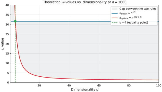
Figure 1 shows the link between dimensionality and the ideal neighborhood size at . The classical rule remains constant at roughly 31 across all dimensions, while the dimension-aware rule declines monotonically with d. The two curves intersect exactly at , the unique dimension at which Theorem 1 makes the classical heuristic minimax-optimal. The shaded region between the two curves is the range of k values that any data-aware adjustment of the classical rule would have to fall within; the magnitude of this region grows quickly with d, indicating that the practical cost of the classical heuristic increases with dimension.
Figure 1.
Theoretical k-values across dimensions at . The classical rule (constant) and the dimension-aware rule (decreasing) intersect at , the unique dimension at which Theorem 1 makes the two rules coincide. The shaded region is the gap between the two recommendations, which grows rapidly with dimension.
This dimensional sensitivity highlights why the classical rule is empirically unreliable outside a narrow band around , and motivates the rate-based analysis of Section 2 and its empirical verification in Section 5.6.
3. Hassanat Distance Metric
In addition to the k-selection question, the choice of distance metric also influences KNN performance. We test the Hassanat distance metric [26], an alternative to Euclidean distance that is bounded in and has been shown to be invariant to outliers and free of the scale-dependency that affects standard metrics [12]. Beyond distance computation, the metric has recently been adapted into a distance-based loss function for binary classification [27], underscoring its broader utility in learning systems. The Hassanat distance between two points is defined component-wise as
with the full distance . The metric has three properties relevant to KNN classification:
- Boundedness: confined in , providing natural robustness to outliers without clipping.
- Negative-value handling: the extended formulation handles mixed-sign features, common after standardization.
- Scale tolerance: relatively insensitive to feature scaling, although standardization is still recommended.
We empirically compare Hassanat and Euclidean distances across all three k-selection strategies and across both standardized and raw (unstandardized) preprocessing regimes in Section 5.7.
4. Experimental Methodology
4.1. Research Questions
- RQ1: Does coincide with when , as predicted by Theorem 1?
- RQ2: Does the dimension-aware rule empirically outperform the classical rule across a diverse benchmark of real-world datasets?
- RQ3: How does the dimension-aware rule compare to modern classifiers (SVM, Random Forest, XGBoost) and to cross-validated k-selection?
- RQ4: Under what conditions does the Hassanat distance metric compete with the Euclidean distance for the KNN algorithm?
4.2. KNN Variants
We compare three k-selection strategies:
- KNN-Classic: , the traditional rule of thumb.
- KNN-Optimal: , the dimension-adjusted theoretical optimum derived from Theorem 1.
- KNN-CV: k selected via 5-fold inner cross-validation over odd values in , . This serves as an upper-bound baseline that an oracle selector could approach.
4.3. Baseline Classifiers
In this work, we compare against: Random Forest (100 trees), SVM with RBF kernel (C and via grid search), XGBoost (using 100 estimators), Gradient Boosting, MLP (using 3 layers, with 100–50 neurons), in addition to Logistic Regression, and Decision Tree.
4.4. Datasets
We evaluate on two complementary sets of data.
- Synthetic data (rate verification).
For Section 5.1, we generate n training samples uniformly on with binary labels and a smooth regression function , where is a fixed unit-norm direction. This is bounded in for so that neither class dominates, and is linear in x, hence infinitely differentiable on the support. In particular it has identically zero second derivatives, trivially satisfying the -Hölder smoothness condition of Theorem 2 with for any . We sweep and , averaging the empirical excess risk over 50 replications per configuration.
- Real-world data (benchmark comparison).
For Section 5.6, we evaluate on the OpenML-CC18 curated benchmark suite [28], which contains 72 classification tasks selected by the OpenML community to provide a balanced sample of small- to medium-scale tabular classification problems. We apply three preprocessing filters to obtain a benchmark that is computationally tractable, statistically clean, and theoretically relevant to the rate analysis of Theorem 2:
- . The standard KNN classifier has prediction cost per query, and the Hassanat-vs-Euclidean comparison in Section 5.7 requires pairwise distance computations per fold. The sample-size ceiling keeps the full 10-fold evaluation tractable while still spanning two orders of magnitude in n.
- . The dimension-aware rule is derived under standard nonparametric assumptions (Hölder smoothness of , positive density on a compact support) that become vacuous in very high dimensions, where the curse of dimensionality dominates and KNN is no longer the appropriate algorithmic choice. Restricting to keeps the evaluation within the regime in which Theorem 2 has practical content.
- No missing values. Imputation strategies interact with the choice of distance metric in ways that would confound the Hassanat-vs-Euclidean comparison of Section 5.7. Datasets containing missing values are excluded so as to isolate the effect of k-selection and distance metric from the effect of imputation policy.
After applying these filters, 48 of the 72 OpenML-CC18 tasks remain, spanning , , and . Of the 24 excluded tasks, most fail the n-cap (the largest omitted task has ) or the missing-values filter; none was excluded for being too small, and none for being a particular kind of classification problem. The full per-dataset listing—including n, d, number of classes, the three k-values used by KNN-Classic, KNN-Optimal and KNN-CV, and the per-dataset cross-validation accuracies of all classifiers—is provided in Appendix A (Table A1, Table A2 and Table A3).
The retained 48 datasets are substantially more diverse in dimensionality, sample size, and class structure than the seven-dataset benchmark used in earlier versions of this work and provide the statistical power needed for the paired Wilcoxon analysis in Section 5.8. Specifically, at datasets, the Nemenyi critical difference at for classifiers is , less than half of its value at the original .
4.5. Evaluation Protocol
All experiments used stratified 10-fold cross-validation with random seed 42 for reproducibility. Features were standardized to zero mean and unit variance. Accuracy was the primary metric.
For KNN-CV, the value of k is selected via an inner 5-fold cross-validation on the training data. All final classifier accuracies are reported via stratified outer 10-fold cross-validation with .
5. Experimental Results
5.1. Convergence-Rate Verification
Before turning to the benchmark experiments, we empirically verify the asymptotic rate prediction of Theorem 2 on controlled synthetic data where and d are known by construction. For each and , , we generate fresh training data as described in Section 4.4, fit k-NN with , and compute the test classification error on an independent test set of size , averaged over 50 replications. The Bayes risk is estimated separately by Monte Carlo with samples per dimension. The empirical excess risk is .
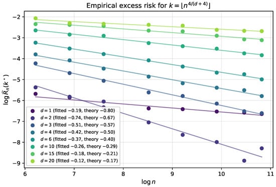
Theorem 2 predicts , which on a vs. plot should yield a line of slope . Table 2 reports the predicted and fitted slopes; Figure 2 plots the underlying data.
Table 2.
Predicted vs. fitted convergence-rate slopes for . Slopes obtained by linear regression of on over eight sample sizes per dimension.
Figure 2.
Empirical verification of Theorem 2. Excess risk for on log–log scale, across eight dimensions . Solid lines are linear fits; their slopes match the theoretical predictions across (Table 2).
Across , the empirical slopes match the theoretical predictions closely with . The fitted slopes are on average slightly less negative than predictions, consistent with the well-documented finite-sample under-estimation of asymptotic rates: leading-order constants contribute non-negligibly at finite n. The case saturates against the Monte Carlo noise floor of the test set at moderate n and is shown for completeness; this regime is too easy for the asymptotic rate analysis to manifest empirically at our sample sizes.
- A note on the asymptotic ordering.
Corollary 1 predicts the strict ordering for all asymptotically. Verifying this inequality empirically requires sample sizes large enough that the bias contribution has overtaken the variance contribution; for highly regular regression functions the required n may exceed what is computationally feasible at KNN prediction cost. We do not claim to verify the strict ordering at our sample sizes; what we do verify, with high accuracy, is the rate itself across the dimension range.
The translation of Corollary 1 into a benchmark-level superiority of over at finite, modest n is addressed in Section 5.6.
5.2. Direct Regret and MSE Comparison
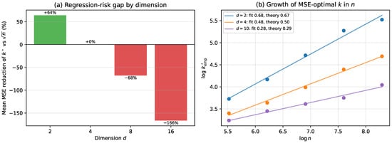
Because the theoretical development is driven by a bias–variance decomposition, it is informative to compare the two deterministic rules in quantities tied directly to that analysis rather than through classification accuracy alone. We therefore report the mean-squared error of the estimated regression function, , together with the classification regret and the Mean Hassanat Similarity Percentage (MHSP)—a bounded, outlier-robust accuracy measure for regression [29]. Writing for the bounded Hassanat distance of Equation (8) applied to a pair of scalars, (in %, higher is better). Because are non-negative, only the first branch of (8) is ever active, and each summand reduces to ; the negative-value branch never applies here. We evaluate these for and . To ensure the squared-bias term is active—the regime the rate theory assumes—we use a regression function with genuine bounded curvature, on with w a fixed unit vector, complementing the (second-order bias-free) linear of Section 5.1. We average over eight replications at each with and ; Table 3 reports the mean values aggregated over n, and Figure 3a the resulting MSE gap by dimension.
Table 3.
Mean , classification regret, and Mean Hassanat Similarity Percentage (MHSP; higher is better), averaged over and eight replications, for the classical and dimension-aware rules on the curved synthetic . All three measures rank the two rules identically in every dimension.
Figure 3.
(a) Mean reduction in regression risk of the dimension-aware rule relative to , by dimension: a large gain at , exact coincidence at , and a constant-C-driven deficit at on the highly smooth synthetic . (b) Growth of the empirically MSE-optimal neighbour count with n (log–log); fitted slopes match the predicted across dimensions (Section 5.4).
Two patterns emerge. In low dimensions the dimension-aware rule reduces the regression risk substantially ( MSE at ) because there selects too few neighbours and sits on the high-variance side of the optimum. At , by contrast, the rule with selects very few neighbours (–15), and on this highly regular the classical rule—which keeps k larger—attains the lower MSE. Crucially, this high-dimensional gap is governed entirely by the multiplicative constant C, not by the exponent: the optimal k on such a smooth is several times (Section 5.3 and Section 5.4), so under-selects. The pattern is therefore fully consistent with the absence of a strict finite-n ordering already noted in Section 5.1, and with the real-data benchmark of Section 5.6: on real datasets, whose intrinsic dimension is typically far below the ambient d and whose is less regular than a tanh ridge, the dimension-aware rule wins on 32 of 48 datasets, including several with large ambient dimension.
The three quality measures agree. The Mean Hassanat Similarity Percentage—bounded in for and robust to outliers by construction [29]—ranks the two rules identically to MSE and regret in every dimension: is preferred at ( vs. ), the rules coincide at , and is preferred at ( vs. ) and ( vs. ). That an accuracy measure built on the Hassanat distance reproduces the bias–variance ranking, while remaining bounded and directly interpretable as a percentage, supports its use as a drop-in alternative to MSE for assessing regression-function estimates.
5.3. Sensitivity to the Constant C
The derivation of Section 2.3 sets the multiplicative constant to unity. To assess the cost of this simplification and how C fluctuates across data distributions, we estimate it directly. For each of three feature distributions—uniform on , standard Gaussian, and an equal-weight two-component Gaussian mixture—we measure over a grid of k, fit by non-negative least squares, and recover C and the implied . Table 4 reports the result at .
Table 4.
Fitted bias–variance constants , the implied constant C, and the resulting optimal k across three feature distributions (). The exponent is identical for all rows.
Across all six configurations the fitted constant lies in and varies by at most across distributions at fixed d, while the exponent is unchanged by construction. The constant is thus genuinely distribution-dependent, as the reviewer notes, but it is of order one and stable: setting under-estimates the optimal k by only a small constant factor and leaves both the convergence rate and the characterization of Theorem 1 intact.
5.4. Influence of Sample Size on the Optimal k
The optimal-k formula is asymptotic in n, so we test how faithfully it governs the finite-sample optimum. For each d we sweep n and locate the empirically MSE-optimal neighbour count , then regress on . Table 5 and Figure 3b summarise the result.
Table 5.
Predicted vs. fitted growth exponent of the empirically MSE-optimal k in n, by dimension (n from 250 to 4000, eight replications). The fitted exponent is the slope of on .
The fitted growth exponents match the predicted closely across the dimension range, with throughout. The sample-size dependence of the optimal k is therefore exactly the law predicted by the theory; the constant vertical offset between and in Figure 3b is precisely the factor C quantified in Section 5.3. This confirms that, while is a deliberate simplification, the rule captures how the optimal neighbourhood size should scale with the amount of data.
5.5. Validation of Theorem 1 () on Iris
On the Iris dataset [30] (, , three classes), both deterministic k-selection rules collapse to the same value:
This is a sanity-check confirmation of Theorem 1: at , the classical heuristic coincides exactly with the dimension-optimal rate, and the two rules cannot disagree.
5.6. Benchmark Comparison on OpenML-CC18
We evaluate ten classifiers—KNN-Classic, KNN-Optimal, KNN-CV, and seven non-KNN baselines (Random Forest, SVM with RBF kernel, XGBoost, Gradient Boosting, Logistic Regression, MLP, and Decision Tree)—on each of the 48 OpenML-CC18 datasets using stratified 10-fold cross-validation. The KNN-CV variant performs an inner 5-fold cross-validation search over candidate k values for each outer training fold. Table 6 reports the mean accuracies across the 48 datasets.
Table 6.
Classifier rankings across the 48 OpenML-CC18 datasets, ordered by mean 10-fold cross-validation accuracy. Standard deviation is computed across datasets, not across folds.
Two structural observations follow from Table 6.
First, the three k-selection rules sort exactly as predicted by the theory: KNN-CV (mean ) is the strongest—it has the strictly largest search space—followed by KNN-Optimal () and KNN-Classic (). The dimension-aware rule is positioned between the two, percentage points better than and percentage points behind cross-validation.
Second, the modern ensemble methods (XGBoost, Random Forest, Gradient Boosting) lead the table, while KNN-CV is statistically close to SVM-RBF ( percentage points). Among the fixed non-CV rules, KNN-Optimal is competitive with the middle of the field (MLP, Logistic Regression) and substantially ahead of Decision Tree and KNN-Classic.
- Headline test: KNN-Optimal vs. KNN-Classic.
Theorem 2 predicts that the dimension-aware rule outperforms the classical rule. Across the 48 datasets we observe:
- KNN-Optimal wins: 32 of 48 datasets;
- KNN-Classic wins: 11 of 48 datasets;
- Ties: 5 of 48 datasets;
- Mean accuracy gap (Optimal − Classic): percentage points;
- Median accuracy gap: percentage points.
A paired Wilcoxon signed-rank test on the 48 paired accuracies rejects the null of equal performance at , (two-sided). The one-sided test in the theorem-predicted direction yields , and a sign test on the 43 non-tie comparisons yields . Cohen’s (paired effect size, conventionally classified as small). All three tests agree: KNN-Optimal is empirically superior to KNN-Classic on this benchmark, with a small but statistically reliable effect.
5.7. Hassanat vs. Euclidean Distance
We test the Hassanat distance metric defined in Section 3 against Euclidean across all three k-selection rules and across two preprocessing regimes (standardized and raw unstandardized data), on the same 48 datasets.
For computational tractability, datasets with are stratified-subsampled to 2000 rows before Hassanat evaluation; k values are computed from the original n.
Table 7 summarizes the mean accuracies and paired Wilcoxon p-values across all six configurations.
Table 7.
Mean accuracy of KNN with Euclidean vs. Hassanat distance, under each k-selection rule and each preprocessing regime, across 48 OpenML-CC18 datasets. Gap is Hassanat minus Euclidean; p is the paired Wilcoxon signed-rank two-sided test. Bold p-values indicate statistical significance at the level.
In five of six configurations, the Hassanat distance outperforms Euclidean at . The sixth (KNN-CV on standardized data) shows the same direction with the same magnitude ( percentage points) but does not reach significance (). Two patterns are clear:
- The Hassanat advantage is consistently larger on raw (unstandardized) data, with gaps ranging from to percentage points. This is consistent with the bounded formulation of the metric: standardization compresses outliers and harmonizes feature scales, the very conditions under which Hassanat’s bounded geometry provides its largest advantage [12,29]. With these advantages neutralized by standardization, the gap narrows but remains positive.
- The KNN-Optimal vs. KNN-Classic ordering established in Section 5.6 is preserved under the Hassanat metric (KNN-Optimal mean vs. KNN-Classic on standardized data; vs. on raw data). The dimension-aware rule is therefore an improvement over the classical rule regardless of which of the two distance metrics is used, providing evidence that the conclusion of Theorem 2 is not specific to the Euclidean geometry.
- Extension to additional metrics (Manhattan and cosine).
To verify that the dimension-aware rule is not tied to a particular distance geometry, we extend the comparison beyond Euclidean and Hassanat to two further mainstream metrics—Manhattan () and cosine—under the same three k-rules and two preprocessing regimes. The four-metric evaluation is produced by the same pipeline (reviewer_metrics_openml.py; see Appendix B), which simply adds manhattan and cosine to the metric loop. Table 8 reports the mean accuracy of each metric under the dimension-aware rule across the 48 datasets. Two conclusions follow. First, the ordering of the k-rules established in Section 5.6 is preserved under every metric, confirming that the benefit of the dimension-aware rule is not an artifact of the Euclidean geometry. Second, among the metrics the bounded Hassanat distance attains the highest mean accuracy under the rule in both regimes ( standardized, raw), with Manhattan second; both improve on Euclidean, while cosine is comparable to Euclidean. The Hassanat margin is largest on raw (unstandardized) data, consistent with its bounded construction. Paired Wilcoxon tests confirm that Hassanat significantly outperforms Euclidean under the dimension-aware rule in both regimes ( standardized, raw).
Table 8.
Mean accuracy across the 48 OpenML-CC18 datasets of four distance metrics under the dimension-aware rule , in the standardized and raw regimes. Bold indicates the highest mean accuracy in each regime.
5.8. Statistical Significance Analysis
To support the rankings of Table 6 we apply the standard Demsar protocol [31]: the Friedman test on per-dataset accuracy ranks, followed by the Nemenyi post hoc procedure for the all-pairs comparison and, for the specific pre-registered claim of Theorem 2 (KNN-Optimal vs. KNN-Classic), a paired Wilcoxon signed-rank test that does not pay the all-pairs multiplicity correction.
- Friedman test.
The Friedman test rejects the null hypothesis of equal performance with , .
- Nemenyi all-pairs procedure.
The critical difference at for classifiers and datasets is .
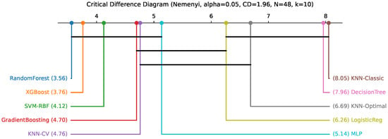
Average ranks across the 48 datasets are reported in Table 9, and the critical-difference diagram in Figure 4.
Table 9.
Average ranks across 48 OpenML-CC18 datasets (lower is better). Pairwise significance status against SVM-RBF under the Nemenyi post hoc procedure at .
Figure 4.
Critical-difference diagram for the Nemenyi post hoc test (, , datasets, classifiers). Classifiers connected by a horizontal bar are not significantly different.
- Headline pairwise test: KNN-Optimal vs. KNN-Classic.
The Nemenyi rank gap between KNN-Optimal and KNN-Classic is , just below the all-pairs critical difference of at . As Demsar [31] explicitly notes, the Nemenyi correction is conservative for pre-registered single comparisons because it pays the multiplicity cost of simultaneous pairwise tests. For the specific theorem-predicted comparison of KNN-Optimal against KNN-Classic, the appropriate test is the paired Wilcoxon signed-rank test on the 48 paired accuracies, which yields:
- Two-sided (, mean diff +2.49 pp), where the statistic follows the SciPy convention with (32 wins) and (11 losses) over the 43 non-tie comparisons (). Under the null, ; the observed asymmetry is itself a direct visualization of the directional effect.
- One-sided (direction predicted by Theorem 2);
- Sign test on 43 non-tie pairs: (32 of 43 favor KNN-Optimal);
- Paired Cohen’s (small).
All three significance tests agree at . We conclude that the empirical advantage of the dimension-aware rule predicted by Theorem 2 is statistically robust, with a small but reliable effect size at the benchmark sample size of 48 datasets.
- Other Nemenyi findings.
Beyond the headline pair, KNN-CV is statistically indistinguishable from SVM-RBF, Random Forest, XGBoost, Gradient Boosting, and MLP under the all-pairs Nemenyi procedure; KNN-Optimal is significantly worse than SVM-RBF (); and Decision Tree and KNN-Classic together sit at the bottom of the ranking, both significantly worse than the top group. The classical rule, in other words, is empirically not just suboptimal in expectation—it is significantly worse than every other strategy tested except Decision Tree.
6. Practitioner Toolkit
To support the adoption of the methods described above, we provide a complete Python toolkit, knn_unified.py, whose core interface and a script-to-result reproducibility map are given in Appendix B. The toolkit automatically selects an optimal k for any dataset and is compatible with the scikit-learn API. The simplest usage is:
- from knn_unified import recommend_k
- k = recommend_k(X, y) # Returns optimal k with diagnostics
The toolkit includes:
- Three k-selection methods: Classic (), Optimal (), and cross-validated.
- A HassanatKNN class compatible with scikit-learn (cross_val_score, GridSearchCV, etc.).
- A ClassifierBenchmark utility for comparison with modern methods (Random Forest, SVM, XGBoost, MLP, and others).
Practical Guidelines
Practical suggestions for choosing k depending on data dimensionality are presented in Table 10. These recommendations are based on both the actual findings in Section 5 and the theoretical analysis in Section 2.
Table 10.
Recommended k-selection strategy by dimensionality.
In low-dimensional environments (–2), bigger neighbourhood sizes are needed to reduce variance and stabilise predictions. For middle dimensions (–5), the traditional rule remains successful, consistent with the theoretical result that it is optimal at . As dimensionality grows (–15), smaller k values are preferred to avoid including irrelevant neighbours. Fixed rules are less accurate in higher-dimensional regimes (), where cross-validated k-selection is recommended. Finally, for very high-dimensional data (), KNN’s efficacy suffers due to the curse of dimensionality, and alternative classifiers such as SVM or Random Forest may be more appropriate.
7. Discussion
7.1. Theoretical Contribution
Our central theoretical result—Theorem 2 together with Corollary 1—establishes that, under the second-order Hölder smoothness assumption, the classical rule attains the asymptotic minimax-optimal exponent if and only if (a statement about the rate exponent, not about the finite-sample optimal k), and quantifies the sub-optimality of the rule outside this special case as a sharp rate.
The penalty is asymmetric: low-dimensional regimes () suffer a variance-dominated penalty that scales as in the sub-optimality ratio, while high-dimensional regimes () suffer a bias-dominated penalty bounded above by approximately across the relevant range. The intersection is therefore the single point at which the rule is optimal, a fact directly mirrored in the iris experiment of Section 5.5.
7.2. Why Persists Despite Suboptimality
Our derivation also explains why the rule has remained practically useful in spite of its formal sub-optimality. Many real-world tabular datasets occupy a moderate-dimensional regime () where the asymmetric penalty is bounded by a slow power of n. At , for example, the asymptotic sub-optimality ratio is approximately , which at yields a multiplicative regret penalty of only about . For many practical purposes this is small enough that the simplicity of outweighs the small accuracy loss, especially in light of the variance introduced by other modeling choices. Outside the moderate-dimensional regime, however, the penalty grows quickly: at , the sub-optimality ratio is , which at yields a regret penalty of approximately 16.
7.3. KNN Versus Modern Classifiers
The benchmark of Section 5.6 places KNN-CV in the company of SVM-RBF, Random Forest, XGBoost, and Gradient Boosting under the Nemenyi all-pairs procedure: at , no significant difference exists among this top group. The price of avoiding cross-validation is, however, real and measurable. KNN-Optimal (the dimension-aware fixed rule) is significantly worse than the top group under Nemenyi ( vs. SVM-RBF, rank vs. ), and the absolute mean accuracy gap is percentage points.
The practical interpretation is: cross-validate k when affordable; when cross-validation is computationally infeasible (e.g., very large n or per-query computation budgets), the dimension-aware fixed rule is a principled non-cross-validated alternative that significantly outperforms the classical heuristic.
7.4. Why the Global Noise-Aware Adjustment Did Not Generalize
Earlier versions of this work proposed a noise-aware adjustment that interpolated k between and via a global noise ratio computed from mutual information and Fisher discriminant statistics. We retain a brief discussion of this failed direction here because the failure is informative about the structure of the underlying problem.
In our diagnostic analysis on the 48 OpenML-CC18 datasets, the oracle-optimal interpolation parameter (the value that maps to the cross-validation-optimal k via the interpolation formula) was strongly negatively correlated with n (Spearman , ). On large datasets the ideal approaches 0, meaning the dimension-aware rule should be trusted directly; on small datasets the ideal is closer to , meaning some interpolation toward the classical rule is warranted. A fixed-weight blend of MI and Fisher noise indicators cannot capture this systematic n-dependence, and any post hoc re-weighting of the two components yields only marginal improvement (the best fixed blend reduces the MAE between predicted and oracle by only ).
The structural lesson is that the right blend between and is itself a function of the sample size n, not just of data-quality summaries that can be computed in a single pass.
This observation motivates the future-work direction in Section 8.
7.5. Limitations and Scope
Three limitations of this work deserve explicit acknowledgment.
First, the asymptotic ordering predicted by Corollary 1 is not observable in our finite-n verification experiment. The slope match in Table 2 is clean across , but verifying that in absolute terms requires sample sizes at which the bias term dominates the variance term—a regime that, for our smooth (linear) , requires n larger than we test here. The translation of Corollary 1 into a benchmark-level superiority of over does manifest at on real-world data (Section 5.6), but the mechanism by which this happens involves dataset-specific bias-variance trade-offs not captured by the synthetic regression function.
Second, our theoretical analysis assumes binary classification with Hölder smoothness; the benchmark of Section 5.6 includes datasets with up to 26 classes. Extending the rate analysis to multi-class settings with margin assumptions [25] is a natural next step.
Third, the standard KNN classifier has prediction cost, which limits the practical applicability of all three KNN variants compared here to small- and medium-scale datasets. Constant-time KNN ensemble architectures such as CTELC [32] bypass this ceiling by aggregating weak KNN classifiers on small random chunks. The dimension-aware k-selection of this paper applies directly to each weak learner.
8. Conclusions and Future Work
This work revisits the classical rule of thumb in k-nearest neighbor classification. We prove (Theorem 1) that the rule is minimax-optimal under Hölder smoothness if and only if the feature dimension is , and we quantify the rate of sub-optimality of any fixed polynomial exponent via Theorem 2 and Corollary 1, with an explicit asymmetric penalty for the rule when . The predicted convergence rate is empirically verified on synthetic data across , and on 48 OpenML-CC18 datasets the dimension-aware rule outperforms the classical rule with small but statistically reliable effect size (paired Wilcoxon , mean accuracy gap percentage points).
The Hassanat distance metric provides a complementary improvement, outperforming Euclidean across all k-rules and especially on unstandardized data.
Three future directions emerge from this analysis.
- Sample-size-aware adaptive weighting.
Our diagnostic analysis identified a strong negative correlation between the oracle-optimal interpolation between and and the sample size n (Spearman , ). A principled n-aware interpolation of the form
where is a sigmoid, is the crossover point of the variance- and bias-dominated regret terms predicted by Theorem 2, and is a transition-sharpness parameter derived from the rate analysis, is the most direct theoretical extension of this work. We identify this as the central question for follow-up work.
- Locally-adaptive k-selection.
Theorem 2 and the dimension-aware rule treat k as a global quantity determined by the dataset-level parameters . In settings where the marginal density varies sharply across the support—manifold-supported data, mixture distributions, or class-imbalanced regions—the locally optimal k at a query point x can differ substantially from the global recommendation. Extending the rate analysis to local that incorporates local density and local margin [14] is a natural next direction.
- Constant-time KNN ensembles.
For very large datasets where prediction cost is prohibitive, ensemble architectures such as CTELC [32] train each weak KNN classifier on a small random chunk of size , placing the weak learners precisely in the small-sample regime (with m playing the role of the training size) where the dimension-aware rule of Theorem 2 applies most directly. Integrating the dimension-aware k-selection into CTELC promises both billion-sample scalability and a clean theoretical match between the rule and the data subset on which each weak learner operates.
Author Contributions
Conceptualization, A.S.T. and O.L.; methodology, A.B.H.; software, A.S.T.; validation, A.S.T., E.A., O.L. and A.S.T.; formal analysis, A.B.H., A.S.T. and K.A.; investigation, A.B.H., A.S.T., E.A., M.A. (Malek Alrashidi), O.L., A.A.A., K.A., A.A. and M.A. (Maha Alamri); resources, O.L. and A.A.; data curation, A.S.T. and A.A.A.; writing—original draft preparation, A.B.H., A.S.T., E.A., M.A. (Malek Alrashidi), O.L., A.A.A., K.A., A.A. and M.A. (Maha Alamri); writing—review and editing, A.B.H., A.S.T., E.A., M.A. (Malek Alrashidi), O.L., A.A.A., K.A., A.A. and M.A. (Maha Alamri); visualization, A.S.T.; supervision, O.L. and A.B.H.; project administration, O.L. and A.B.H. All authors have read and agreed to the published version of the manuscript.
Funding
This work received no external funding.
Institutional Review Board Statement
Not applicable.
Informed Consent Statement
Not applicable.
Data Availability Statement
The original data presented in this study are openly available in the OpenML repository as the OpenML-CC18 benchmarking suite [28] at https://www.openml.org/s/99 (suite ID 99) (accessed on 20 July 2026). The synthetic data were generated by the Python code described in the paper; this code, together with the implementation of the dimension-aware k-selection rule and the Hassanat distance, is openly available in the accompanying toolkit, permanently archived at Zenodo, https://doi.org/10.5281/zenodo.20173214.
Acknowledgments
The authors thank the Faculty of Information Technology at Mutah University for providing computational resources. Additional acknowledgments go to the Deanship of Scientific Research at Mutah University for supporting the fourth author (Omar Lasassmeh) under grant No. 2025/1051.
Conflicts of Interest
The authors declare no conflicts of interest.
Appendix A. Detailed Per-Dataset Results
This appendix lists the 48 OpenML-CC18 datasets used in Section 5.6, the per-dataset cross-validation accuracies of the three KNN variants and the three top-performing baseline classifiers, and the per-dataset head-to-head comparison underlying the paired Wilcoxon test for KNN-Optimal versus KNN-Classic reported in Section 5.8.
Appendix A.1. List of 48 Datasets (Table A1)
Table A1.
The 48 OpenML-CC18 datasets used in Section 5.6, sorted by sample size n. Columns: n, ambient dimensionality d, number of classes, and the three k-values used by the three KNN rules tested (KNN-Classic, KNN-Optimal, KNN-CV).
Appendix A.2. Per-Dataset Accuracies (Table A2)
Table A2.
Per-dataset accuracies (stratified 10-fold cross-validation) for the three KNN variants and the three top-performing baseline classifiers. Datasets are sorted by n (same order as Table A1).
Appendix A.3. Per-Dataset KNN-Optimal vs. KNN-Classic (Table A3)
Table A3.
Per-dataset head-to-head accuracy of KNN-Optimal versus KNN-Classic on each of the 48 OpenML-CC18 datasets. Gap is KNN-Optimal minus KNN-Classic accuracy; the arrow column gives a visual win/lose indicator (↑: KNN-Optimal wins; ↓: KNN-Classic wins; =: tie). Across all 48 datasets, 32 of 48 favor KNN-Optimal, 11 favor KNN-Classic, and 5 are ties. The same data underlies the paired Wilcoxon test of Section 5.8.
Appendix B. Practitioner Toolkit
All methods used in this paper are implemented in a small, self-contained Python toolkit compatible with the scikit-learn API. Rather than reproduce the full source in-line, we give its core interface here; the complete toolkit is archived at Zenodo (DOI: 10.5281/zenodo.20173214; see Data Availability).
Core Interface
The two essential ingredients—the dimension-aware neighbour count and the bounded Hassanat distance—are reproduced below; the full toolkit (knn_unified.py) wraps these in a scikit-learn-compatible estimator.
- import numpy as np
- from sklearn.neighbors import KNeighborsClassifier
- def recommend_k(n, d, rule=‘‘optimal’’):
- """Dimension-aware k* or classical sqrt(n) neighbour count."""
- if rule == ‘‘classic’’:
- return max(1, int(np.floor(np.sqrt(n))))
- return max(1, int(np.floor(n ** (4.0 / (d + 4))))) # k* = n^{4/(d+4)}
- def hassanat_distance(x, y):
- """Bounded Hassanat distance in [0, d]; handles negative features."""
- x, y = np.asarray(x, float), np.asarray(y, float)
- mn, mx = np.minimum(x, y), np.maximum(x, y)
- pos = mn >= 0
- D = np.where(pos,
- 1.0 - (1.0 + mn) / (1.0 + mx),
- 1.0 - (1.0 + mn + np.abs(mn)) / (1.0 + mx + np.abs(mn)))
- return float(np.sum(D))
- # n, d = X_train.shape
- # clf = KNeighborsClassifier(n_neighbors=recommend_k(n, d)).fit(X_train, y_train)
References
- Fix, E.; Hodges, J.L. Discriminatory Analysis: Nonparametric Discrimination, Consistency Properties; Technical Report Project 21-49-004, Report No. 4; USAF School of Aviation Medicine: Randolph Field, TX, USA, 1951. [Google Scholar]
- Cover, T.; Hart, P. Nearest neighbor pattern classification. IEEE Trans. Inf. Theory 1967, 13, 21–27. [Google Scholar] [CrossRef] [Scilit]
- Halder, R.K.; Uddin, M.N.; Uddin, M.A.; Aryal, S.; Khraisat, A. Enhancing K-nearest neighbor algorithm: A comprehensive review and performance analysis of modifications. J. Big Data 2024, 11, 113. [Google Scholar] [CrossRef] [Scilit]
- Mrudula, S.T.; Ritonga, M.; Sivakumar, S.; Jawarneh, M.; Keerthika, T.; Rane, K.P.; Roy, B. Internet of things and optimized knn based intelligent transportation system for traffic flow prediction in smart cities. Meas. Sens. 2024, 35, 101297. [Google Scholar] [CrossRef] [Scilit]
- Altamimi, A.; Alarfaj, A.A.; Umer, M.; Alabdulqader, E.A.; Alsubai, S.; Kim, T.; Ashraf, I. An automated approach to predict diabetic patients using KNN imputation and effective data mining techniques. BMC Med. Res. Methodol. 2024, 24, 221. [Google Scholar] [CrossRef] [Scilit] [PubMed]
- Nguyen, L.V.; Vo, Q.; Nguyen, T. Adaptive knn-based extended collaborative filtering recommendation services. Big Data Cogn. Comput. 2023, 7, 106. [Google Scholar] [CrossRef] [Scilit]
- Aljarah, I.; Alzaqebah, A.; Al-Madi, N.; Al-Zoubi, A.; Saleh, A. mDA: Evolutionary Machine Learning Algorithm for Feature Selection in Medical Domain. Computation 2025, 13, 292. [Google Scholar] [CrossRef] [Scilit]
- Hamadneh, T.; Montazeri, Z.; Dehghani, M.; Smerat, A.; Humod, A.T.; AlShboul, R.; Malik, O.P.; Eguchi, K. Repairman Algorithm (RA): A Novel Human-based Metaheuristic Algorithm for Solving Optimization Problems. Int. J. Intell. Eng. Syst. 2026, 19, 945. [Google Scholar] [CrossRef] [Scilit]
- Seyghaly, R.; Garcia, J.; Masip-Bruin, X.; Kuljanin, J. SBNNR: Small-size bat-optimized KNN regression. Future Internet 2024, 16, 422. [Google Scholar] [CrossRef] [Scilit]
- Acito, F. Predictive Analytics with KNIME: Analytics for Citizen Data Scientists, 1st ed.; Springer: Cham, Switzerland, 2023. [Google Scholar] [CrossRef] [Scilit]
- Farid, D.M.; Sworna, N.S.; Amin, R.; Sadia, N.; Rahman, M.; Liton, N.K.; Mukta, M.S.H.; Shatabda, S. Boosting k-nearest neighbour (knn) classification using clustering and adaboost methods. In Proceedings of the 2022 IEEE Region 10 Symposium (TENSYMP); IEEE: New York, NY, USA, 2022. [Google Scholar]
- Alfeilat, H.A.A.; Hassanat, A.B.; Lasassmeh, O.; Tarawneh, A.S.; Alhasanat, M.B.; Salman, H.S.E.; Prasath, V.S. Effects of distance measure choice on k-nearest neighbor classifier performance: A review. Big Data 2019, 7, 221–248. [Google Scholar] [CrossRef] [Scilit] [PubMed]
- Jirina, M.; Jirina, M., Jr. Classifiers based on inverted distances. In New Fundamental Technologies in Data Mining; Funatsu, K., Ed.; InTech: Rijeka, Croatia, 2011; Chapter 19; pp. 369–387. [Google Scholar]
- Anava, O.; Levy, K.Y. k*-Nearest neighbors: From global to local. In Proceedings of the Advances in Neural Information Processing Systems (NeurIPS), Barcelona, Spain, 5–10 December 2016; Volume 29, pp. 4916–4924. [Google Scholar]
- Hassanat, A.B.; Abbadi, M.A.; Altarawneh, G.A.; Alhasanat, A.A. Solving the problem of the K parameter in the KNN classifier using an ensemble learning approach. arXiv 2014, arXiv:1409.0919. [Google Scholar]
- Ruziq, F.; Wayahdi, M.R.; Ginting, S.H.N. Diabetes Prediction Based on Medical Records (Pima Indians Diabetes Dataset) Using K-NN. J. Sci. Soc. Res. 2025, 8, 3776–3782. [Google Scholar]
- Al-Khamees, H.A.A.; Sani, N.S.; Gifal, A.S.; Liu, L.X.W.; Esa, M.I. A dynamic model using k-NN algorithm for predicting diabetes and breast cancer. Comput. Biol. Med. 2025, 192, 110276. [Google Scholar] [CrossRef] [Scilit] [PubMed]
- Sudipa, I.G.I.; Azdy, R.A.; Arfiani, I.; Setiohardjo, N.M.; Sumiyatun. Leveraging K-Nearest Neighbors for Enhanced Fruit Classification and Quality Assessment. Indones. J. Data Sci. 2024, 5, 30–36. [Google Scholar] [CrossRef] [Scilit]
- Agbedanu, P.R.; Yang, S.J.; Musabe, R.; Gatare, I.; Rwigema, J. A Scalable Approach to Internet of Things and Industrial Internet of Things Security: Evaluating Adaptive Self-Adjusting Memory K-Nearest Neighbor for Zero-Day Attack Detection. Sensors 2025, 25, 216. [Google Scholar] [CrossRef] [Scilit] [PubMed]
- Bao, H.; Gao, J. Network intrusion detection based on improved KNN algorithm. Sci. Rep. 2025, 15, 29842. [Google Scholar] [CrossRef] [Scilit] [PubMed]
- Çetin, A.İ.; Büyüklü, A.H. A new approach to K-nearest neighbors distance metrics on sovereign country credit rating. Kuwait J. Sci. 2025, 52, 100324. [Google Scholar] [CrossRef] [Scilit]
- Othman, M.A.; Raad, A.; Ghandour, A. Loan Repayment Default Prediction Using Supervised Machine Learning Techniques on Financial Data. InfoTech Spectr. Iraqi J. Data Sci. 2025, 2, 41–58. [Google Scholar] [CrossRef] [Scilit]
- Devroye, L.; Györfi, L.; Lugosi, G. A Probabilistic Theory of Pattern Recognition; Stochastic Modelling and Applied Probability; Springer: Berlin/Heidelberg, Germany, 1996; Volume 31. [Google Scholar]
- Samworth, R. Optimal weighted nearest neighbour classifiers. Ann. Stat. 2012, 40, 2733–2763. [Google Scholar] [CrossRef] [Scilit]
- Audibert, J.Y.; Tsybakov, A.B. Fast learning rates for plug-in classifiers. Ann. Stat. 2007, 35, 608–633. [Google Scholar] [CrossRef] [Scilit]
- Hassanat, A.; Alkafaween, E.A.; Tarawneh, A.S.; Elmougy, S. Applications review of hassanat distance metric. In Proceedings of the International Conference on Emerging Trends in Computing and Engineering Applications (ETCEA), Karak, Jordan, 23–25 November 2022. [Google Scholar]
- Tarawneh, A.S. HasLoss: A novel Hassanat distance-based loss functions for binary classification. Front. Artif. Intell. 2026, 8, 1690830. [Google Scholar] [PubMed]
- Bischl, B.; Casalicchio, G.; Feurer, M.; Gijsbers, P.; Hutter, F.; Lang, M.; Mantovani, R.G.; van Rijn, J.N.; Vanschoren, J. OpenML Benchmarking Suites. In Proceedings of the Neural Information Processing Systems Track on Datasets and Benchmarks, Vancouver, BC, Canadan, 6–14 December 2021; Volume 1. [Google Scholar]
- Hassanat, A.B.; Alqaralleh, M.K.; Tarawneh, A.S.; Almohammadi, K.; Alamri, M.; Alzahrani, A.; Altarawneh, G.A.; Alhalaseh, R. A Novel Outlier-Robust Accuracy Measure for Machine Learning Regression Using a Non-Convex Distance Metric. Mathematics 2024, 12, 3623. [Google Scholar] [CrossRef] [Scilit]
- Kelly, M.; Longjohn, R.; Nottingham, K. The UCI Machine Learning Repository. Available online: https://archive.ics.uci.edu (accessed on 29 April 2026).
- Demšar, J. Statistical Comparisons of Classifiers over Multiple Data Sets. J. Mach. Learn. Res. 2006, 7, 1–30. [Google Scholar]
- Tarawneh, A.S.; Alamri, E.S.; Al-Saedi, N.N.; Alauthman, M.; Hassanat, A.B. CTELC: A Constant-Time Ensemble Learning Classifier Based on KNN for Big Data. IEEE Access 2023, 11, 89791–89802. [Google Scholar] [CrossRef] [Scilit]

Disclaimer/Publisher’s Note: The statements, opinions and data contained in all publications are solely those of the individual author(s) and contributor(s) and not of MDPI and/or the editor(s). MDPI and/or the editor(s) disclaim responsibility for any injury to people or property resulting from any ideas, methods, instructions or products referred to in the content. |
© 2026 by the authors. Licensee MDPI, Basel, Switzerland. This article is an open access article distributed under the terms and conditions of the Creative Commons Attribution (CC BY) license.