A Method for 6-DOF Motion Measurement of Marine Floating Structures Based on Monocular Vision and Feature Point Tracking

Abstract

Accurate measurement of the 6-DOF motion responses of marine floating structures is essential for structural safety assessment and operational decision-making. To address the critical issues of integration drift in inertial navigation systems, susceptibility of GNSS to sea-surface multipath effects, and deployment complexity of binocular vision systems, this paper proposed a 6-DOF motion measurement method for floating structures based on monocular vision and natural feature point tracking. This method eliminates the reliance on artificial cooperative targets and auxiliary sensors, instead utilizing the inherent surface textures of the floating structures as feature sources. Stable feature point tracking is achieved through multi-strategy cascaded detection and the pyramidal KLT optical flow algorithm. RANSAC geometric consistency verification is introduced to eliminate outlier matches, retaining only identical physical points between two consecutive frames for motion estimation. In-plane translations and $RZ$ angle are extracted from the similarity transformation, while $RX$ and $RY$ angles are estimated using principal component analysis of the covariance matrix of the feature point set. The depth-direction displacement is linearly mapped from variations in the scale factor. Subsequently, two series of physical model tests under different conditions were conducted to validate the measurement accuracy and robustness of the proposed method on different floating structures. The results demonstrate that the proposed method can accurately capture the motion attitudes of floating structures, maintaining a consistently high inlier ratio exceeding 80% in regular waves and averaging 85.2% in irregular waves, with a reprojection error of less than 0.05 pixels. The NRMSE for the primary motion directions are all below 10%, and the dominant frequency errors are essentially zero. It offers advantages such as low cost, easy deployment, and strong robustness, thereby providing valuable technical support for field monitoring of marine floating structures.

1. Introduction

With the continuous depletion of land resources and the ever-increasing global energy demand, the development and utilization of marine resources have become an important strategic direction to alleviate the supply–demand contradiction [1,2]. To expand the frontiers of marine space utilization, various marine floating structures have been rapidly developed, including floating wind turbines [3], deep-water semi-submersible platforms [4], and offshore floating photovoltaic systems, which have attracted considerable attention in recent years [5]. Unlike onshore structures, the marine environment is characterized by the coupling of multiple dynamic factors such as wind, waves, and currents. During their service life, floating structures are subjected to complex and variable external excitations, exhibiting large-amplitude six-degree-of-freedom (6-DOF) motion responses [6,7]. These motions not only impair the operational safety and fatigue life of the structures but also significantly reduce the efficiency of onboard equipment. Under extreme sea conditions, they may even cause mooring system failure or overall structural capsizing [8]. Therefore, accurate measurement of the 6-DOF motion response of floating structures in real ocean environments is of great significance for optimizing structural design, evaluating operational status, and formulating maintenance strategies [9].

Currently, motion monitoring of marine floating structures mainly relies on the combination of an inertial navigation system (INS) and a global positioning system (GPS) [10,11]. In such a system, the INS uses accelerometers and gyroscopes to measure acceleration and angular velocity, from which displacement and attitude are obtained through integration. However, due to unknown initial conditions, sensor bias drift, and environmental noise, the double integration of acceleration to obtain displacement is prone to severe drift. Even after filtering, the low-frequency drift components cannot be completely removed [12]. Liu et al. [13] demonstrated that a low-cost micro-electro-mechanical system (MEMS)-based INS without external correction can experience a position drift exceeding 10 m within 10 min. Meanwhile, global navigation satellite system (GNSS) positioning methods also face significant challenges in marine environments. Jiang et al. [14] found through field tests that multipath effects caused by sea-surface reflection can increase GNSS positioning errors by two to three times compared with land environments, reaching 0.4–0.8 m in open seas. Furthermore, signal interruption caused by structural occlusion and extreme weather further limits the reliability and accuracy of GNSS in monitoring the motions of marine floating structures [15,16].

With the rapid progress of computer vision, image-based non-contact measurement methods have gained increasing attention in ocean engineering owing to their advantages, such as eliminating the need to install sensors on the target structure and requiring only simple data acquisition equipment [17,18]. In the field of binocular or multi-view stereo vision, Xu et al. [19] proposed a stereo vision-based 6-DOF motion measurement system for offshore floating photovoltaic platforms. They employed the YOLOv5 deep learning model for target detection and achieved sub-pixel localization through ellipse fitting, validating the measurement accuracy under both regular and irregular wave conditions. Liang et al. [20] proposed a fully automated visual method for measuring TLCD/TLCGD displacement by integrating spatiotemporal continuity constraints with physics-based modal priors. Wang et al. [21] developed a high-precision 6-DOF motion capture method based on image recognition, using three shipborne cameras to capture real-time video of a fixed jacket frame and achieving target tracking through a multi-scale template matching algorithm. Their method attained centimeter-level positioning accuracy and angular accuracy better than 0.1° in offshore float-over installation operations. Yi et al. [22] developed an optical-based multi-target three-dimensional dynamic motion measurement system and conducted on-site evaluation on large concrete floating structures, further demonstrating the feasibility of vision-based measurement for prototype marine structures. Guo et al. [23] recently proposed a large displacement measurement method by integrating deep learning-based RAFT optical flow with the classical KLT method, which jointly considers pixel-level and subpixel-level motions to improve measurement accuracy. The causal-guided adaptive multimodal diffusion network proposed by Cai et al. [24] has demonstrated the capability of integrating complementary information from multiple sources for enhanced domain adaptation. However, a comparative study by Kang et al. [25] demonstrated that, under long-range observation, monocular vision yields lower measurement error than stereo vision, indicating that monocular vision offers unique advantages in long-distance marine monitoring scenarios.

In the field of monocular vision-based motion measurement, early research can be traced back to 2011, when some scholars attempted to estimate the 6-DOF motion parameters of small ship models from single-camera image sequences, paving the way for non-contact marine structural monitoring [26]. In recent years, the rapid development and engineering application of deep learning have significantly enhanced the anti-interference capability of monocular vision in target detection, feature matching, and motion tracking. Jeon et al. [27] proposed using convolutional neural networks to automatically track cables and autonomously redefine regions of interest. Nguyen et al. [28] integrated a traditional KLT tracker with a deep learning model to develop a vision-based method for measuring structural displacement, which enhanced the robustness and accuracy of detection when the line of sight is obstructed or lighting conditions are poor. Xia et al. [29] developed a monocular vision-based safety monitoring framework utilizing Grounded SAM, enabling accurate target detection, instance segmentation, and distance estimation for offshore infrastructures, with advantages such as low cost and easy deployment. Moreover, camera calibration is of critical importance in monocular vision-based measurement. Zhou et al. [30] proposed a fisheye camera calibration model that achieves mean reprojection errors of 1.6 and 1.8 pixels in the X- and Y-directions, respectively. Nevertheless, most existing monocular vision methods still rely on artificial cooperative targets [31,32,33]. For large-scale marine floating structures in service, attaching artificial markers not only involves risks associated with working at height and high maintenance costs, but may also damage the surface anti-corrosion coating and structural integrity, hindering the widespread application of such methods in practical engineering.

Based on the foregoing review, the following limitations can be identified in existing motion estimation methods for floating structures: (1) most methods rely on cooperative targets, making them difficult to apply to practical engineering structures where attaching artificial targets is not feasible or desirable; (2) binocular or multi-view schemes require the synchronized calibration and deployment of at least two cameras, resulting in high system complexity and poor field adaptability; (3) although deep-learning-based monocular methods have progressed in target detection, they still lack a systematic theoretical solution for refined 6-DOF motion estimation. Therefore, developing a 6-DOF motion measurement method that requires only a single camera and does not rely on artificial targets remains a research gap that urgently needs to be addressed in ocean engineering.

To fill this gap, this paper proposed a 6-DOF motion measurement method for marine floating structures based on monocular vision and feature point tracking. The core novelties of this work are as follows: (1) a systematic integration pipeline that achieves marker-less 6-DOF motion estimation using only a monocular camera; (2) a covariance PCA-based method that establishes an analytical mapping from the statistical distribution of feature points in the image plane to the roll and pitch angles, which decouples the estimation of out-of-plane rotations from the similarity transformation of point correspondences and provides a purely geometric alternative that does not rely on prior structural models or depth assumptions; and (3) a multi-strategy cascaded feature detection scheme to address the challenges of real marine environments, including water-surface reflections, rapid large-amplitude motions induced by waves, and frequent occlusions. The core idea is to use the natural textures on floating structures’ surfaces as feature sources. Stable tracking is achieved through multi-strategy feature point detection (Minimum Eigenvalue, SURF, FAST) combined with the KLT optical flow method. Outliers caused by water-surface reflections, occlusions, and other factors are eliminated through Random Sample Consensus (RANSAC) geometric consistency verification, and only those feature points successfully tracked across consecutive frames are retained for subsequent motion estimation. For motion parameter estimation, in-plane translation and $RZ$ angle are directly extracted from the similarity transformation. $RX$ and $RY$ angles are estimated by performing principal component analysis on the covariance matrix of the feature point set, using variations in the principal direction angle and aspect ratio. The depth-direction displacement is linearly mapped from the variation in the scale factor. Table 1 summarizes the key differences between the proposed method and representative existing approaches.

Table 1. Comparison of the proposed method with representative vision-based methods.

Aspect	Proposed Method	Stereo-Vision	Monocular with Targets
Feature source	Natural textures	Artificial markers	Artificial markers
Prior model required	No	No	Yes
Outlier rejection	RANSAC + bidirectional KLT	Epipolar constraint + RANSAC	RANSAC
6-DOF estimation	Similarity transform + PCA	3D reconstruction + PnP	PnP
Deployment	Single camera, any position	Two + cameras, fixed baseline	Single camera, targets pre-installed

The remainder of this paper is organized as follows. Section 2 details the feature point detection and tracking methods, including Region of Interest (ROI) initialization, multi-strategy feature point detection, and KLT optical flow tracking. Section 3 elaborates the 6-DOF motion parameter estimation method, with emphasis on roll and pitch estimation based on principal component analysis of the covariance matrix. Section 4 validates the accuracy of the proposed method and the influence of distance through regular wave tests in a wave flume. Section 5 evaluates the robustness of the method through irregular wave tests in a wave basin. Section 6 concludes the paper and provides an outlook on future work.

2. Feature Point Detection and Tracking for Floating Structures

2.1. Overview of Monocular Vision Measurement Method

The proposed measurement system comprises two main components: a monocular camera and the floating structure under test. The camera is rigidly mounted, with its optical axis directed toward the anticipated motion region of the floating structure, and captures a continuous image sequence of the structural motion. The inherent natural textures on the floating structure’s surface, such as paint patterns, bolt holes, and weld seams, are utilized as feature sources, eliminating the need to attach any artificial markers. The entire measurement process relies solely on monocular image sequences, without the aid of inertial sensors, GNSS, or stereo vision devices.

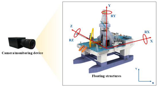
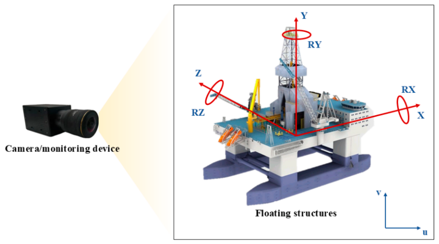
To describe the motion of the floating structure in a unified manner, two coordinate systems are defined as follows, as shown in Figure 1. (1) Image coordinate system $O-uv$: the origin is located at the upper-left corner of the image, with the $u$-axis pointing horizontally to the right and the $v$-axis pointing vertically upward. (2) Physical world coordinate system $W-XYZ$: the origin is set at the camera optical center, with the $X$-axis pointing horizontally to the right (parallel to the $u$-axis), the $Y$-axis pointing vertically upward (parallel to the $v$-axis), and the $Z$-axis along the camera optical axis (depth direction), following the right-hand rule. Since the camera is fixed, the world coordinate system coincides with the camera coordinate system. The floating structure is treated as a rigid body, with the relative positions among feature points on its surface remaining invariant during motion. The spatial distribution of feature points in the first frame is taken as the baseline topology, against which all subsequent frame-to-frame variations are compared for motion estimation. Therefore, the projection of a physical point on the floating structures surface onto the image plane follows the perspective projection model. The 6-DOF motion parameters of the floating structure are then determined by analyzing the variations in the feature point projections between consecutive frames.

Figure 1. Schematic diagram of the coordinate systems.

Let the image sequence captured by the monocular camera be denoted as ${\left\{I_k\right\}}_{k=0}^{K-1}$, where $k$ is the frame index and $K$ is the total number of frames. The set of valid feature points in the $k$-th frame is defined as $P_k={\left\{P_i^k\right\}}_{i=1}^{N_k}$, with $P_i^k={\left(u_i^k,v_i^k\right)}^T$ representing the pixel coordinates of the $i$-th feature point. Successfully matched point pairs between consecutive frames form a match set ${\mathcal{M}}_k=\left\{\left(P_i^k,P_i^{k+1}\right)\right\}$, under the constraint that $P_i^k$ and $P_i^{k+1}$ correspond to the same physical point in space. The overall measurement pipeline comprises, in sequence, ROI initialization, multi-strategy feature detection, KLT optical flow tracking, bidirectional error checking, RANSAC geometric consistency verification, and feature point re-detection. Details of each component are presented in the following subsections.

2.2. Feature Point Detection and Initialization

In the first frame $I_0$, a polygonal region $\Omega$ that encloses the main body of the floating structure is selected interactively, and an indicator function is defined as:

$${\mathbb{I}}_{\Omega }\left(P\right)=\left\{\begin{array}{c}1,P\in \Omega \\ 0,P\notin \Omega \end{array}\right.$$

(1)

All subsequent operations are restricted within $\Omega$ to exclude interference from water surface waves and the background shoreline. To accommodate floating structures surfaces with different texture conditions, this paper adopts a multi-strategy cascade detection method, which is executed in the following order until the number of detected points meets the minimum requirement $N_{min}$:

(1) Shi–Tomasi corners (Minimum Eigenvalue): Compute the minimum eigenvalue of the image gradient structure tensor and select points that are local maxima. For a pixel point $(u,v)$, within the neighborhood $\mathcal{W}$ of point $P_i^k$, constructs the autocorrelation matrix:

$$M=\left[\begin{array}{cc}{\sum }_{(u,v)\in \mathcal{W}}{I}_u^2& {\sum }_{(u,v)\in \mathcal{W}}{I}_u{I}_v\\ {\sum }_{(u,v)\in \mathcal{W}}{I}_u{I}_v& {\sum }_{(u,v)\in \mathcal{W}}{I}_v^2\end{array}\right]$$

(2)

where $I(u,v)$ is the image intensity function, $I_u=\partial I/\partial u$ and $I_v=\partial I/\partial v$ are the image intensity gradients in the $u$ and $v$ directions, respectively. Let ${\eta }_1$, ${\eta }_2$ be the two eigenvalues of $M$, then the corner response is $S=\mathrm{m}\mathrm{i}\mathrm{n}({\eta }_1,{\eta }_2)$. Points with $S$ greater than a threshold and that are local maxima are selected as Minimum Eigenvalue feature points.

(2) SURF feature: Detect blob-like extremal points based on the determinant of the Hessian matrix, which is robust to scale changes. At scale $\sigma$, the Hessian matrix is:

$$U=\left[\begin{array}{cc}{L}_{uu}(u,v,\sigma )& L_{uv}(u,v,\sigma )\\ L_{uv}(u,v,\sigma )& L_{vv}(u,v,\sigma )\end{array}\right]$$

(3)

where $L_{uu}$ denotes the convolution of the Gaussian second-order partial derivative ${\displaystyle \frac{{\partial }^2}{{\partial u}^2}}g(\sigma )$ with the image $I$, and similarly for $L_{uv}$ and $L_{vv}$. Compute the determinant $\mathrm{d}\mathrm{e}\mathrm{t}\left(U\right)$ and take its local maximum points as SURF feature points.

(3) FAST feature: Rapidly detect corners by comparing intensity differences in contiguous pixels on a circular neighborhood. Taking a candidate point $p$ as the center, if there exists a set of $n$ contiguous pixels whose intensities are all greater than $I\left(p\right)+\zeta$ or all smaller than $I\left(p\right)-\zeta$ ($\zeta$ is the intensity difference threshold), then $p$ is considered a corner.

Detailed derivations of the above three methods can be found in [34,35,36]. The resulting feature point set for the first frame is $P_0={\left\{P_i^0\right\}}_{i=1}^{N_0}$.

2.3. Inter-Frame Tracking and Bidirectional Error Checking

For adjacent frames $I_k$ and $I_{k+1}$, the pyramid-based KLT optical flow algorithm is used to estimate the displacement of feature points. Compared with the traditional optical flow method. The KLT algorithm decomposes large-displacement motion into multiple small-displacement motions by constructing an image pyramid, and performs optical flow computation level by level, thus avoiding the tracking failure problem that tends to occur when the floating structures moves at a high speed. KLT is based on the brightness constancy assumption, i.e., the pixel intensities within a local neighborhood of the same physical point remain unchanged between frames. Then, its corresponding point $P_i^{k+1}$ should satisfy:

$$I_{k+1}\left(P_i^{k+1}+q\right)=I_k\left(P_i^k+q\right),\forall q\in \mathcal{W}$$

(4)

where $q={(∆u,∆v)}^T$ is the pixel displacement vector within $\mathcal{W}$.

Performing the first-order Taylor expansion of the left-hand side of Equation (4) at frame $k$ and neglecting higher-order terms yields the optical flow constraint equation:

$$I_u∆u+I_v∆v+I_t=0$$

(5)

where $I_t=\partial I/\partial t$ is the temporal gradient, and $\left(∆u,∆v\right)=P_i^{k+1}-P_i^k$ is the displacement to be determined.

For all pixels within the window $\mathcal{W}$, Equation (5) constitutes an overdetermined linear system. To obtain a robust solution, a weighted least-squares scheme is introduced. Suppose there are $m$ pixels inside the window, and construct matrix $A$ and vector $B$ as follows:

$$A=\left[\begin{array}{cc}{I}_u^1& I_v^1\\ ⋮& ⋮\\ I_u^m& I_v^m\end{array}\right],B=-\left[\begin{array}{c}{I}_t^1\\ ⋮\\ I_t^m\end{array}\right]$$

(6)

Let the weight matrix be $W=diag({\omega }_1,\dots ,{\omega }_m)$, where ${\omega }_j=exp\left(-{\displaystyle \frac{{(u_j-u_0)}^2+{(v_j-v_0)}^2}{2{\sigma }^2}}\right)$ is the Gaussian weight. Then the weighted least-squares solution is given by:

$$\left[\begin{array}{c}∆u\\ ∆v\end{array}\right]={\left(A^{T}WA\right)}^{-1}{A}^{T}Wb$$

(7)

By employing a pyramid multi-level structure and solving iteratively from the top level (coarse resolution) down to the bottom level (original resolution), large-displacement motion can be handled.

Forward tracking alone is susceptible to mismatches caused by occlusions and illumination variations. To address this, a bidirectional error checking scheme is adopted in this paper: the points in $P_k$ are first tracked forward to frame $k+1$, yielding a candidate set ${\tilde{P}}_{k+1}$; then, using ${\tilde{P}}_{k+1}$ as the starting points, they are tracked backward to frame $k$, producing a back-projected point set $P_k^{back}$. For each point pair, the backward error $e$ can be computed as:

$$e_i={‖P_i^k-P_i^{back}‖}_2$$

(8)

where $e_i$ denotes the backward error (Euclidean distance) of the $i$-th feature point. If $e_i$ exceeds a preset threshold $E_{max}$, the match is considered unreliable and is discarded. Point pairs that pass the bidirectional check constitute the initial match set ${\tilde{\mathcal{M}}}_k=\left\{\left(P_i^k,P_i^{k+1}\right)\right\}$. In this way, only the same physical points that are successfully matched across two consecutive frames and satisfy the consistency condition are retained for subsequent computation.

2.4. Geometric Consistency Verification and Feature Point Management

Even after the bidirectional check, ${\tilde{\mathcal{M}}}_k$ may still contain erroneous matches (outliers) caused by specular reflections off the water surface, partial occlusions, or motion blur. To eliminate the influence of outliers, this paper adopts the RANSAC algorithm to fit a similarity transformation model between the matched point pairs [37]. A similarity transformation comprises rotation, uniform scaling, and translation, with a total of four degrees of freedom. Its homogeneous coordinate form is:

$$\left[\begin{array}{c}{u}_i^{k+1}\\ v_i^{k+1}\\ 1\end{array}\right]=\left[\begin{array}{ccc}{s}_k·\mathit{cos}\theta & -s_k·\mathit{sin}\theta & t_{u,k}\\ s_k·\mathit{sin}\theta & s_k·\mathit{cos}\theta & t_{v,k}\\ 0& 0& 1\end{array}\right]\left[\begin{array}{c}{u}_i^k\\ v_i^k\\ 1\end{array}\right]$$

(9)

where $s_k$ and $t_k={\left(t_{u,k},t_{v,k}\right)}^T$ denote the scale factor and the translation vector of the $k$-th frame, respectively, and $\theta$ is the rotation angle. Equation (9) can be written as:

$$P_i^{k+1}=s_k\left[\begin{array}{cc}\mathit{cos}\theta & -\mathit{sin}\theta \\ \mathit{sin}\theta & \mathit{cos}\theta \end{array}\right]P_i^k+t_k$$

(10)

RANSAC estimates the transformation parameters by randomly sampling the minimal set of point pairs (two pairs) and classifies each matched point pair as an inlier or outlier based on its residual. The residual is defined as the Euclidean distance between the actual position and the position predicted by the transformation:

$$r_i={‖P_i^{k+1}-(s_k\left[\begin{array}{cc}\mathit{cos}\theta & -\mathit{sin}\theta \\ \mathit{sin}\theta & \mathit{cos}\theta \end{array}\right]P_i^k+t_k)‖}_2$$

(11)

If $r_i$ is smaller than the inlier distance threshold $d_{in}$, the point pair is considered an inlier; otherwise, it is an outlier.

To determine the required number of iterations, a probabilistic model is introduced. Let $p_{in}$ denote the proportion of inliers. The probability that a single random sample of two point pairs consists entirely of inliers is $p_{in}^2$. After $T$ independent sampling trials, the probability of obtaining at least one successful sample is:

$$P_s=1-{(1-p_{in}^2)}^T$$

(12)

Given a desired confidence level $P_d=0.995$, the minimum required number of iterations is:

$$T={\displaystyle \frac{\mathrm{l}\mathrm{o}\mathrm{g}(1-P_d)}{\mathrm{l}\mathrm{o}\mathrm{g}(1-p_{in}^2)}}$$

(13)

After multiple iterations, the transformation model with the largest number of inliers is retained, and the final transformation parameters are re-estimated using all inliers. Denote the inlier index set by ${\mathcal{L}}_k$. A closed-form least-squares solution based on singular value decomposition (SVD) is adopted to improve numerical stability. The mean-centered matrices are constructed as:

$$H=\sum _{i\in {\mathcal{L}}_k}(P_i^k-{\overline{P}}^k)(P_i^{k+1}-{\overline{P}}^{k+1}{)}^T\in {\mathbb{R}}^{2\times 2}$$

(14)

where ${\overline{P}}^k$ and ${\overline{P}}^{k+1}$ are the centroids of the respective point sets.

Performing singular value decomposition on $H$ yields $H=U\sum V^T$. The scale factor and translation vector can then be expressed as:

$$\left\{\begin{array}{c}{s}_k={\displaystyle \frac{t_r\left(\sum \right)}{{\sum }_{i\in {\mathcal{L}}_k}{‖P_i^k-{\overline{P}}^k‖}^2}}\\ t_k={\overline{P}}^{k+1}-s_k\left[\begin{array}{cc}\mathit{cos}\theta & -\mathit{sin}\theta \\ \mathit{sin}\theta & \mathit{cos}\theta \end{array}\right]{\overline{P}}^k\end{array}\right.$$

(15)

This method directly provides the transformation parameters, avoiding nonlinear iterations.

The reliable matched pairs used for motion estimation can be expressed as:

$${\mathcal{M}}_k^{inlier}=\left\{\right(P_i^k,P_i^{k+1}\left)\right|i\in {\mathcal{L}}_k\}$$

(16)

The inlier ratio is defined as:

$$r_{in}^k={\displaystyle \frac{\left|{\mathcal{L}}_k\right|}{\left|{\tilde{\mathcal{M}}}_k\right|}}$$

(17)

The average reprojection error can be expressed as:

$${ϵ}_{RMS}^k=\sqrt{{\displaystyle \frac{1}{\left|{\mathcal{L}}_k\right|}}\sum _{i\in {\mathcal{L}}_k}{r}_i^2}$$

(18)

These two indicators serve as quantitative bases for evaluating the tracking quality of each frame. When $r_{in}^k$ decreases significantly or ${ϵ}_{RMS}^k$ increases, it suggests that the current frame may have suffered severe interference, and re-detection is triggered.

During motion, some feature points may be permanently lost due to moving out of the field of view or changes in surface texture. To maintain a sufficient number of tracked points, the system dynamically supplements new features. Denote the current set of active feature points, consisting of the inlier points in the current frame (with coordinates in the $k$-th frame), as $P_k^{active}$. When $\left|P_k^{active}\right|<N_{min}$, re-detection is triggered: the multi-strategy feature point detection described in Section 2.2 is re-executed within the region $\Omega$, and the newly detected points are merged with the remaining active points to form a new $P_{k+1}$.

The above process constitutes a complete monocular vision feature point tracking system. The ROI definition in the first frame and multi-strategy detection ensure sufficient initial features; KLT optical flow together with bidirectional verification achieves stable inter-frame matching; RANSAC geometric consistency verification removes outliers, retaining only the same physical points successfully matched across two consecutive frames for motion computation; and the re-detection mechanism ensures continuity of long-term tracking. The final output reliable matched pairs ${\mathcal{M}}_k^{inlier}$ serve as the direct input for the 6-DOF motion parameter estimation presented in Section 3.

3. Calculation of Motion Parameters for Floating Structures Based on Image Sequences

3.1. Extraction of Planar Motion and Depth Displacement Based on Similarity Transformation

Section 2 obtains the similarity transformation parameters between consecutive frames using RANSAC and the SVD closed-form solution, and defines the inlier index set ${\mathcal{L}}_k$ based on ${\mathcal{M}}_k^{inlier}$. To convert from pixel units to physical units, three calibration coefficients ${\gamma }_X,{ \gamma }_Y$ and ${\gamma }_Z$ are defined as the conversion factors in the horizontal, vertical, and depth directions, respectively.

The linear mapping between depth displacement and scale factor variation is derived from the perspective projection model. The image scale $s$ of a given object is inversely proportional to its distance Z from the camera along the optical axis, i.e., $s\propto 1/Z$. Under high-frame-rate sampling, the depth displacement $∆Z_k$ between consecutive frames is typically small. A first-order Taylor expansion yields $∆Z_k\propto (s_{k+1}-s_k)$. Therefore, the depth displacement can be expressed as a linear function of the change in the scale factor. Since the first frame is taken as the reference with a normalized scale, $(s_{k+1}-s_k)$ reduces to $s_k-1$ in the incremental calculation, and the proportional coefficient is denoted as ${\gamma }_Z$.

The incremental 6-DOF motions between adjacent frames can then be directly expressed as:

$$\left[\begin{array}{c}∆X_k\\ ∆Y_k\\ ∆Z_k\\ ∆{\psi }_k\end{array}\right]=\left[\begin{array}{cccc}{\gamma }_X& 0& 0& 0\\ 0& {\gamma }_Y& 0& 0\\ 0& 0& {\gamma }_Z& 0\\ 0& 0& 0& 1\end{array}\right]\left[\begin{array}{c}\begin{array}{c}{t}_{u,k}\\ t_{v,k}\end{array}\\ \begin{array}{c}{s}_k-1\\ {\psi }_k\end{array}\end{array}\right]$$

(19)

In Equation (19), $∆X_k$ and $∆Y_k$ are directly mapped from the translation components, $∆Z_k$ is linearly mapped from the change in the scale factor, and the $RZ$ angle increment $∆{\psi }_k$ is exactly the rotation angle itself.

3.2. $RX$ and $RY$ Calculation Based on Covariance Principal Component Analysis

When floating structures undergoes roll or pitch motion, the spatial distribution of its projected point set on the image plane changes correspondingly. To quantify such changes, this paper develops a method based on principal component analysis (PCA) of the covariance matrix of the feature point set, which calculates the attitude angles by exploiting the variation in the spatial distribution of the feature points.

For the $k$-th frame, the inlier index set is ${\mathcal{L}}_k$, i.e., ${\left\{P_i^k\right\}}_{i\in {\mathcal{L}}_k}$. The centroid of the point set ${\overline{P}}^k$, can be expressed as:

$${\overline{P}}^k={\displaystyle \frac{1}{\left|{\mathcal{L}}_k\right|}}\sum _{i\in {\mathcal{L}}_k}{P}_i^k=\left[\begin{array}{c}{\overline{u}}_k\\ {\overline{v}}_k\end{array}\right]$$

(20)

The mean-centered coordinate matrix is constructed as $X_k=[P_1^k-{\overline{P}}^k,\dots ,P_{\left|{\mathcal{L}}_k\right|}^k-{\overline{P}}^k]\in {\mathbb{R}}^{2\times \left|{\mathcal{L}}_k\right|}$, and the covariance matrix can be expressed as:

$$C_k={\displaystyle \frac{1}{\left|{\mathcal{L}}_k\right|-1}}{X}_k{X}_k^T=\left[\begin{array}{cc}{C}_{uu,k}& C_{uv,k}\\ C_{uv,k}& C_{vv,k}\end{array}\right]$$

(21)

where $C_{uu,k}$, $C_{uv,k}$ and $C_{vv,k}$ can be expressed as:

$$\left\{\begin{array}{c}{C}_{uu,k}={\displaystyle \frac{1}{\left|{\mathcal{L}}_k\right|-1}}{\displaystyle \sum _{i\in {\mathcal{L}}_k}}{(u_i^k-{\overline{u}}_k)}^2\\ C_{vv,k}={\displaystyle \frac{1}{\left|{\mathcal{L}}_k\right|-1}}{\displaystyle \sum _{i\in {\mathcal{L}}_k}}{(v_i^k-{\overline{v}}_k)}^2\\ C_{uv,k}={\displaystyle \frac{1}{\left|{\mathcal{L}}_k\right|-1}}(u_i^k-{\overline{u}}_k)(v_i^k-{\overline{v}}_k)\end{array}\right.$$

(22)

The eigenvalues ${\lambda }_{1,k}\ge {\lambda }_{2,k}>0$ of the covariance matrix $C_k$ satisfy the characteristic equation $\mathit{det}\left(C_k-\lambda I\right)=0$, whose solutions are:

$$\begin{array}{c}{\lambda }_{1,k}={\displaystyle \frac{1}{2}}\left(C_{uu,k}+C_{vv,k}+\sqrt{{(C_{uu,k}-C_{vv,k})}^2+{4C}_{uv,k}^2}\right)\\ {\lambda }_{2,k}={\displaystyle \frac{1}{2}}\left(C_{uu,k}+C_{vv,k}-\sqrt{{(C_{uu,k}-C_{vv,k})}^2+{4C}_{uv,k}^2}\right)\end{array}$$

(23)

The corresponding eigenvectors can be expressed as:

$$\begin{array}{c}{V}_{1,k}=\left[\begin{array}{c}{\lambda }_{1,k}-C_{vv,k}\\ C_{uv,k}\end{array}\right]\\ V_{2,k}=\left[\begin{array}{c}{C}_{uv,k}\\ {\lambda }_{2,k}-C_{uu,k}\end{array}\right]\end{array}$$

(24)

After normalization, the angle of the first principal direction can be expressed as:

$${\alpha }_k=arctan2({\left(V_{1,k}\right)}_y,{\left(V_{1,k}\right)}_x)$$

(25)

The aspect ratio of the point set is defined as:

$${\beta }_k={\displaystyle \frac{{\lambda }_{2,k}}{{\lambda }_{1,k}}},0\le {\beta }_k\le 1$$

(26)

Within the PCA framework, the projection of the feature point set can be approximated as an ellipse. The orientation of this ellipse is dominated by the rotation ($RY$ motion) about the $Y$-axis, which directly manifests as an overall rotation of the point cloud in the image plane. Therefore, the change in the principal direction angle ${\alpha }_k$ primarily reflects the $RY$ increment ${∆\theta }_k$. In contrast, the rotation ($RX$ motion) about the $X$-axis produces a foreshortening effect in the projection, which alters the distribution of the point cloud along the principal axis without changing its orientation. This effect is mainly reflected in the aspect ratio ${\beta }_k$ (the ratio of the eigenvalues ${\lambda }_2/{\lambda }_1$ of the covariance matrix). Consequently, for small angular increments between consecutive frames, the change in ${\alpha }_k$ can be used to estimate the $RY$ increment, and the change in ${\beta }_k$ can be used to estimate the $RX$ increment. The sign of the off-diagonal element $C_{uv,k}$ of the covariance matrix indicates the direction of rotation. Accordingly, the $RY$ angle increment ${∆\theta }_k$ and the $RX$ angle increment $∆{\varphi }_k$ between adjacent frames can be respectively calculated as:

$$\begin{array}{c}∆{\varphi }_k={\gamma }_{\varphi }·({\alpha }_{k+1}-{\alpha }_k)\\ {∆\theta }_k={\gamma }_{\theta }·({\beta }_{k+1}-{\beta }_k)\end{array}$$

(27)

where ${\gamma }_{\varphi }$ and ${\gamma }_{\theta }$ are proportional coefficients determined by experimental calibration. The sign of the off-diagonal element $C_{uv,k}$ of the covariance matrix indicates the direction of rotation. Defining the sign function ${sgn}_k=sign\left(C_{uv,k}\right)$, Equation (27) can be rewritten as:

$$\begin{array}{c}∆{\varphi }_k={\gamma }_{\varphi }·{sgn}_k·|{\alpha }_{k+1}-{\alpha }_k|\\ {∆\theta }_k={\gamma }_{\theta }·{sgn}_k·|{\beta }_{k+1}-{\beta }_k|\end{array}$$

(28)

To suppress small noise perturbations, dead-zone thresholds ${\varphi }_{min}$ and ${\theta }_{min}$ are introduced. When $|∆{\varphi }_k|<{\varphi }_{min}$ and $\left|{∆\theta }_k\right|<{\theta }_{min}$, the corresponding increments are set to zero.

3.3. Accumulation of Motion Increments and Filtering-Based Smoothing

After the six motion increments for each frame are obtained, the absolute motion parameters relative to the initial pose in the first frame are obtained by accumulation, which can be expressed as:

$$\begin{array}{ccc}{X}_k={\displaystyle \sum _{j=1}^k}∆X_j& Y_k={\displaystyle \sum _{j=1}^k}∆Y_j& Z_k={\displaystyle \sum _{j=1}^k}∆Z_j\\ {\varphi }_k={\displaystyle \sum _{j=1}^k}∆{\varphi }_j& {\theta }_k={\displaystyle \sum _{j=1}^k}{∆\theta }_j& {\psi }_k={\displaystyle \sum _{j=1}^k}∆{\psi }_j\end{array}$$

(29)

The raw motion sequence inevitably contains high-frequency jitter caused by water surface fluctuations, illumination variations, or tracking noise. To extract physically meaningful motion trends, a first-order infinite impulse response (IIR) low-pass filter is adopted for real-time smoothing. For any degree of freedom $q_k$, the filtered output ${\tilde{q}}_k$ satisfies the recurrence relation:

$${\tilde{q}}_k=a{q}_k+(1-a){\tilde{q}}_{k-1}$$

(30)

where $a\in \left(0,1\right)$ is the filtering coefficient. The transfer function of the filter is $F\left(z\right)=a/[1-(1-a\left)z^{-1}\right]$, which provides significant attenuation for high-frequency components.

In addition, to evaluate the overall measurement quality of each frame, a composite metric is constructed using the inlier ratio $r_{in}^k$ and the average reprojection error ${ϵ}_{RMS}^k$ defined in Section 2:

$$Q_k=r_{in}^k·exp\left(-{\displaystyle \frac{{ϵ}_{RMS}^k}{{ϵ}_0}}\right)$$

(31)

where ${ϵ}_0$ is a reference error. The closer $Q_k$ is to 1, the more reliable the tracking.

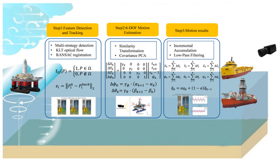
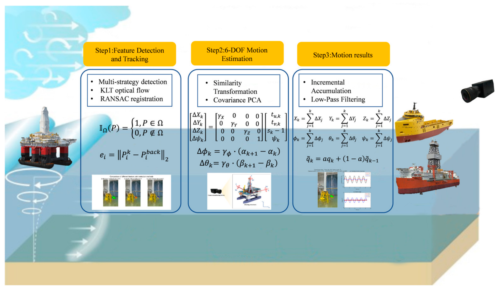
Thus, the proposed method has fully established the analytical relationship from monocular image sequences to the 6-DOF motion parameters of the floating structures, as shown in Figure 2. Section 4 and Section 5 validate the measurement accuracy and robustness of the method through physical model tests in a wave flume and a wave tank, respectively.

Figure 2. Overall workflow of the proposed method.

4. Experimental Validation by Physical Model Tests in the Wave Flume

To validate the accuracy and robustness of the proposed method, scale-model tests were conducted on a jacket-type combined wind-wave energy converter in a wave flume. Using the results from a high-precision optical motion capture system as the reference, the measurement accuracy, tracking stability, and generalization capability of the proposed method under various wave conditions were evaluated.

4.1. Wave Flume Experimental Setup

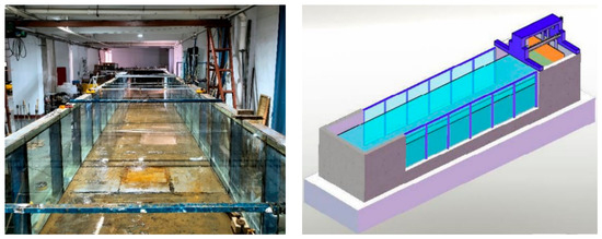
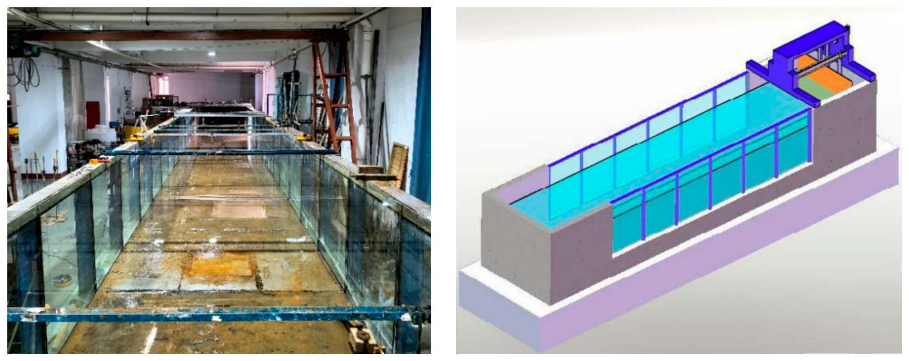
The experiments were carried out in the wave flume at the Shandong Provincial Key Laboratory of Ocean Engineering, Ocean University of China. The flume is 60 m long, 3 m wide, and 1.5 m deep. One end is equipped with a piston-type wave maker capable of generating both regular waves and JONSWAP irregular waves, with a wave period ranging from 0.5 s to 2 s and a maximum wave height of 0.25 m. The other end is furnished with a wave-absorbing mesh, as shown in Figure 3. To minimize the influence of wave reflection and sidewall effects on the generated waves, the model was positioned 25 m from the wavemaker.

Figure 3. Wave flume.

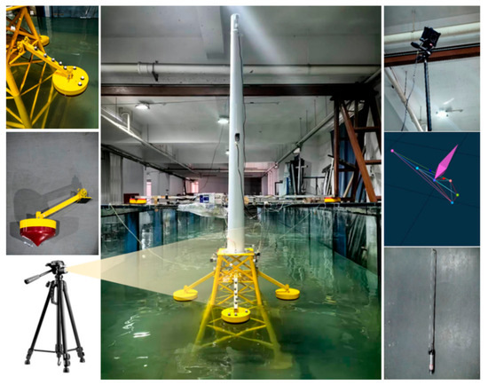
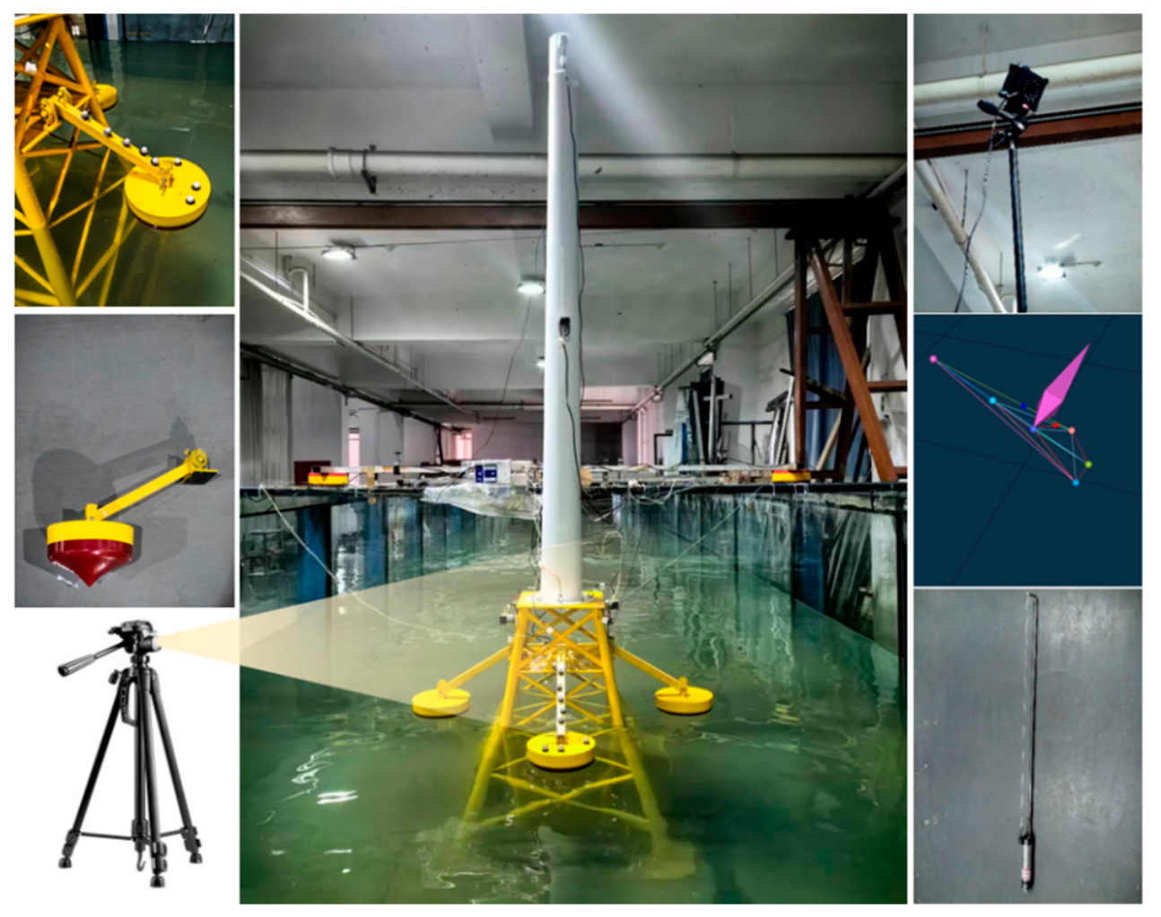
The scale model of the jacket-type combined wind–wave energy converter was designed according to the Froude similarity criterion at a scale ratio of 1:40. The main structure was fabricated from 304 stainless steel, with a tower height of 2.125 m and a jacket foundation height of 1.125 m. Three oscillating buoys with swing arms were mounted on the second-level deck of the foundation, at a height of 0.175 m above the still water surface. The swing arm and the buoy were rigidly connected with no relative displacement between them; the arm length was 0.3 m, and in the static state it formed an angle of 26.3° with the horizontal plane. In this experiment, the world coordinate system was defined as follows: the $X$-axis was along the direction of wave propagation, the $Y$-axis points vertically upward, and the $Z$-axis follows the right-hand rule. The overall experimental arrangement is shown in Figure 4.

Figure 4. Wave flume experimental setup.

The primary measurement instruments included: (1) a NOKOV optical three-dimensional motion capture system (NOKOV Science & Technology Co., Ltd., China), which was used to monitor the motion response of the swing-arm buoys in real time at a sampling frequency of 500 Hz. Four high-resolution Mars-series cameras were deployed, each with a maximum resolution of 26 megapixels and a maximum frame rate of 380 fps. The system captured the infrared light reflected by eight irregularly placed markers on the wave-facing buoy and derived their spatial coordinates and rotation information. (2) Capacitance-type wave gauges (China), together with an SG2000 data acquisition unit, were used for real-time wave monitoring to verify the accuracy of the target wave height generated by the wave maker. (3) A monocular camera (China) with a resolution of 1080× 1920 pixels and a frame rate of 30 fps was fixed outside the flume, with its optical axis directed toward the motion region of the buoys.

4.2. Measurement Accuracy Verification

Prior to the experiment, calibration was performed using marker points with known physical distances on the floating structures. Since the spacings between the optical motion capture marker balls attached to the buoy surface were known, the pixel distances between these markers in the initial frame were measured, which allowed the establishment of a linear mapping between the image coordinates and the world coordinates, thereby yielding the conversion coefficients ${\gamma }_X$ and ${\gamma }_Y$ for the $X$ and $Y$ directions. The calibration coefficient for the depth direction, i.e., the $Z$-axis, was estimated by translating the target through a known distance along the optical axis and measuring the resulting change in the scale factor. For experiments conducted at different camera-target distances (e.g., 1.6 m and 3.5 m in Section 4.3), the coefficient ${\gamma }_Z$ was recalibrated independently at each distance, as the relationship between the scale factor variation and the physical depth displacement depends on the absolute depth.

The recorded video files were read frame by frame using the VideoReader function in MATLAB. For each frame, the procedures described in Section 2 were executed in sequence: ROI delineation, multi-strategy feature point detection, KLT optical flow tracking, and RANSAC geometric consistency verification. Subsequently, following the motion parameter calculation method presented in Section 3, the translation, rotation, and scale changes were extracted from the similarity transformation between consecutive frames and, after conversion by the calibration coefficients, the 6-DOF motion time histories were output.

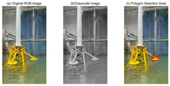
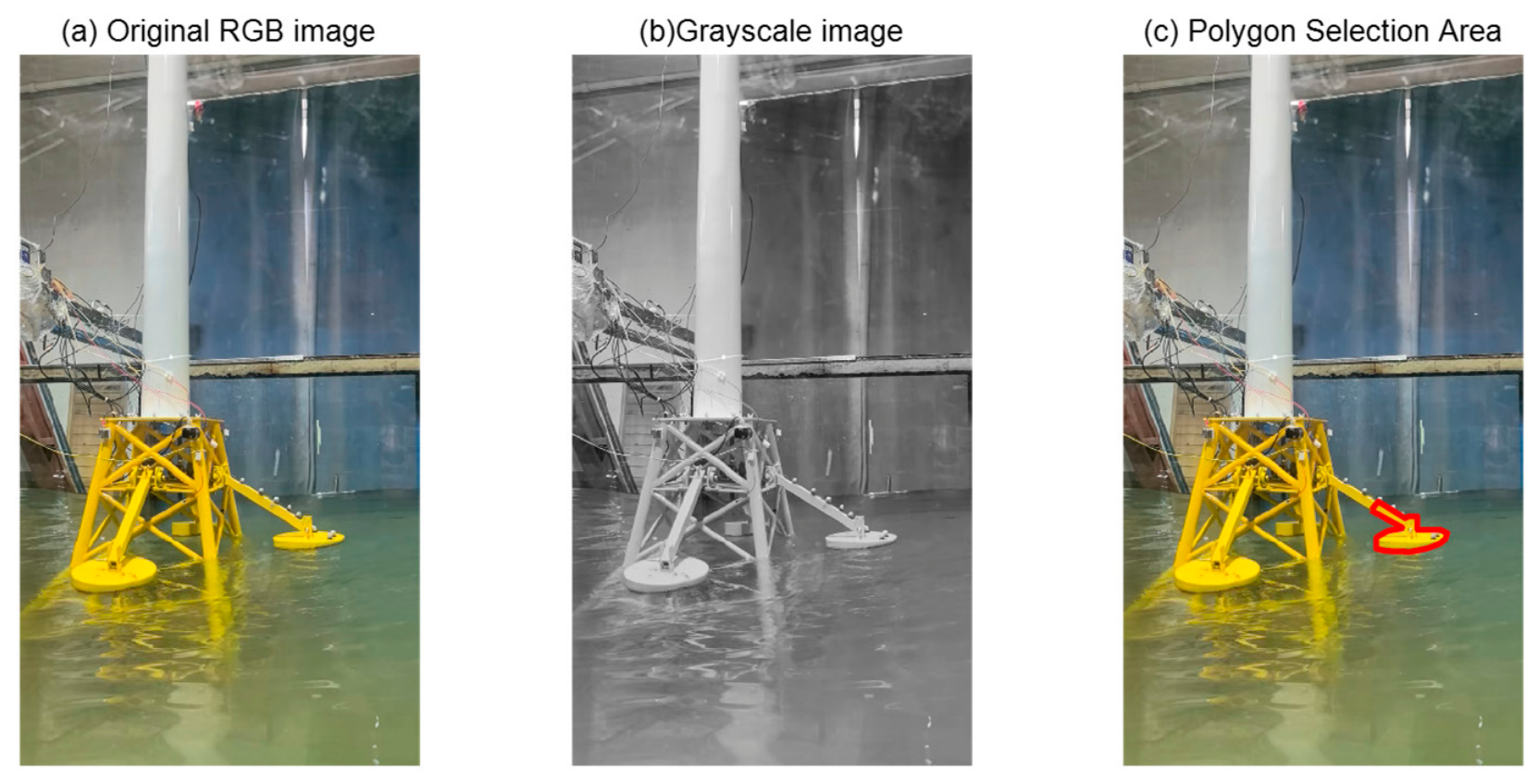
In the first frame, to eliminate interference from water surface waves and the background shoreline, it was necessary to initialize a polygonal ROI enclosing the main body of the buoy. Compared with a conventional rectangular ROI, a polygonal ROI can more precisely conform to the irregular contour of the buoy. The vertex coordinates of this region were recorded and a binary mask was generated. All subsequent feature point detection and tracking operations were strictly confined within this mask region. Figure 5a shows the original RGB image, Figure 5b the grayscale image, and Figure 5c the result after superimposing the polygonal mask, where the ROI precisely delineates the buoy area and effectively isolates background interference.

Figure 5. Polygonal ROI and image initialization.

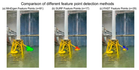
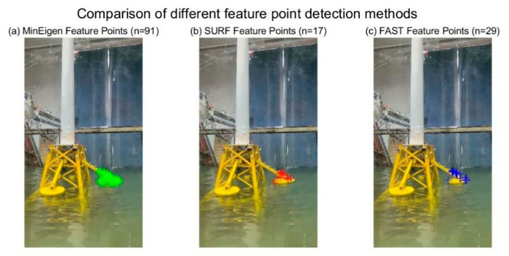
To accommodate floating structures surfaces with different texture conditions, this paper employs a multi-strategy cascade detection method to obtain the initial feature points. Figure 6 compares the outputs of three detectors, Minimum Eigenvalue, SURF, and FAST, within the same ROI. The Minimum Eigenvalue corners (Figure 6a) yielded 91 feature points, exhibiting the most uniform distribution and concentrating in texture-rich regions. The SURF detector (Figure 6b) produced only 17 points; although it possessed good scale invariance, the point count is too low to ensure the robustness of the subsequent motion parameter calculation. The FAST detector (Figure 6c) detected 29 points, but they exhibited noticeable local clustering. Considering the requirement for a uniform spatial distribution of points in the subsequent tracking stage, this paper selected the Minimum Eigenvalue corners as the initial feature point set.

Figure 6. Comparison of feature point detection results among Minimum Eigenvalue, SURF, and FAST.

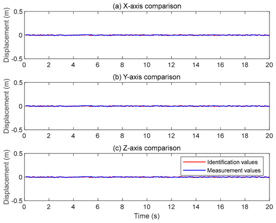
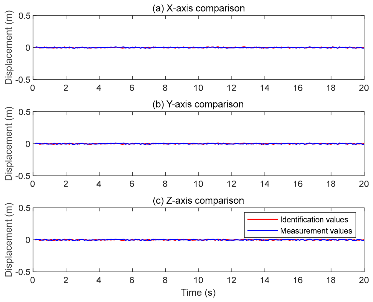
With the camera and the floating structures both kept stationary, a 20 s video was continuously recorded to evaluate the static levels of electronic noise, ambient illumination fluctuations, and feature point detection errors of the system. The standard deviations of the displacement in the $X$, $Y$, and $Z$ directions computed by the proposed method were 0.05 mm, 0.07 mm, and 0.42 mm, respectively, indicating that the system exhibited satisfactory static stability, as shown in Figure 7.

Figure 7. Static stability test.

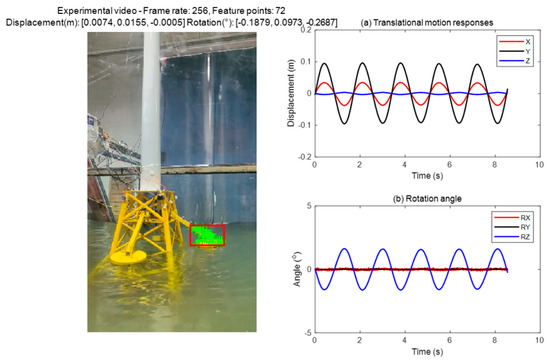
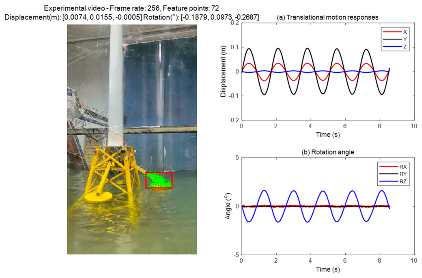
A regular wave condition with a wave height of 0.08 m and a period of 1.7 s was selected for dynamic response identification. Under the Froude scale ratio of 1:40, this condition corresponds to an extreme sea state for the target application site—the coastal waters of northern China—to validate the method’s measurement capability under large-amplitude motions. The straight-line distance between the camera and the buoy was 1.6 m. After the buoy motion reached a steady periodic state under wave action, a 20 s video was recorded, and the reference data from the NOKOV optical motion capture system were synchronously acquired for accuracy comparison. The identification process is shown in Figure 8.

Figure 8. 6-DOF motion identification of the buoy.

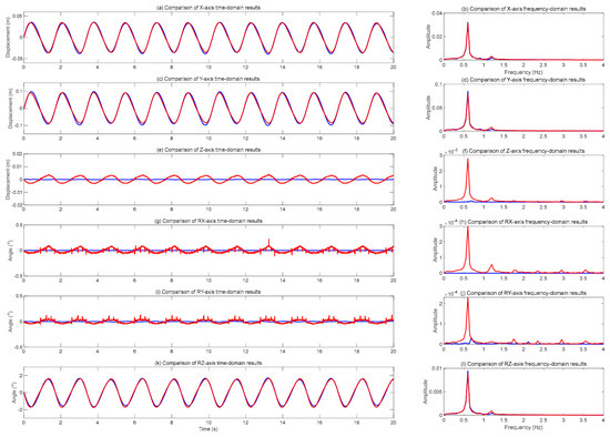
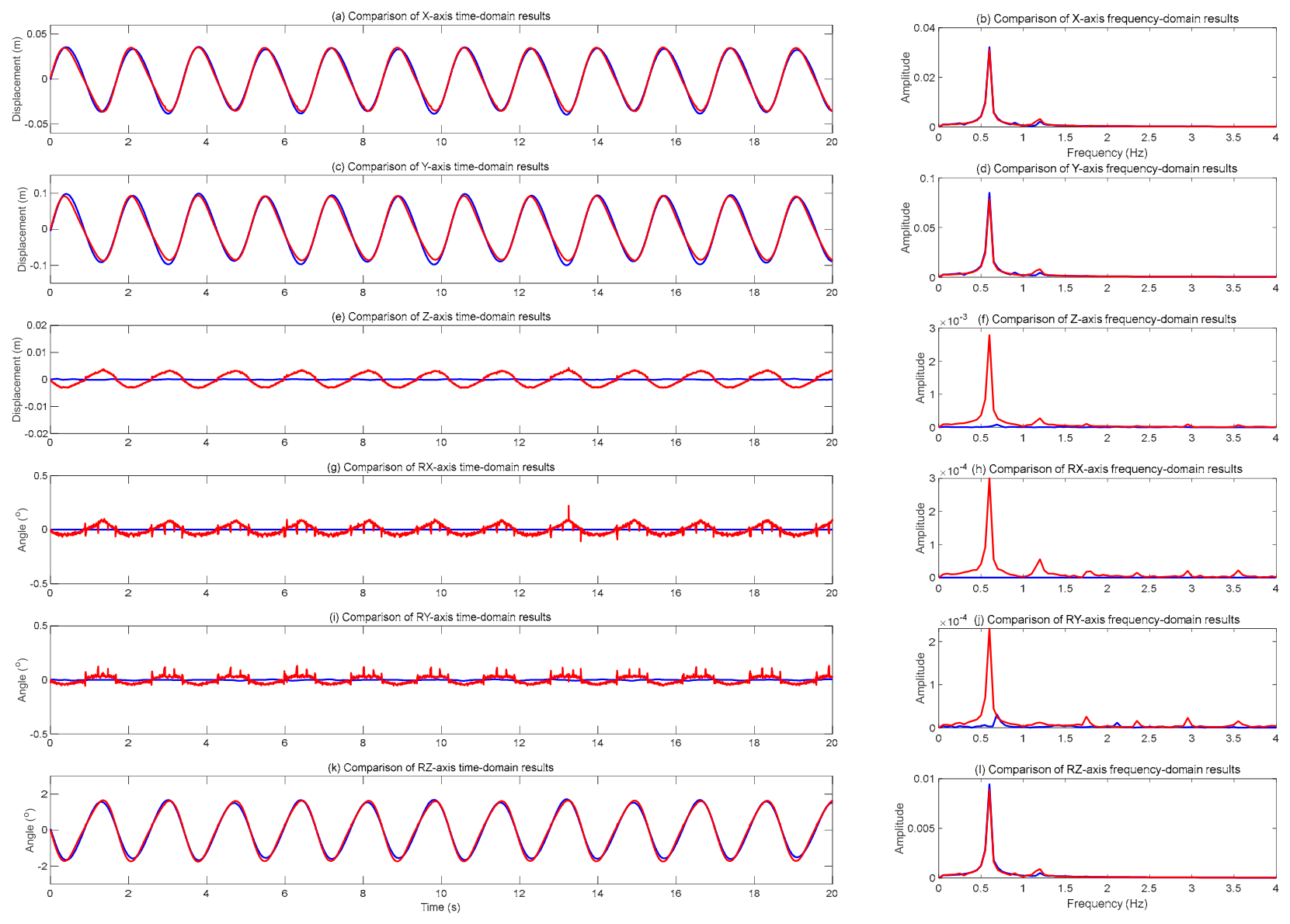
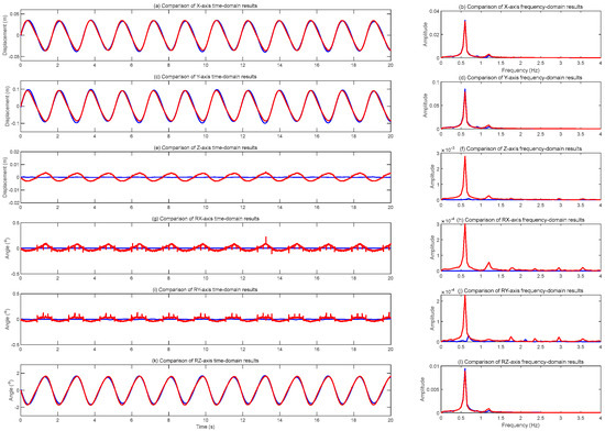
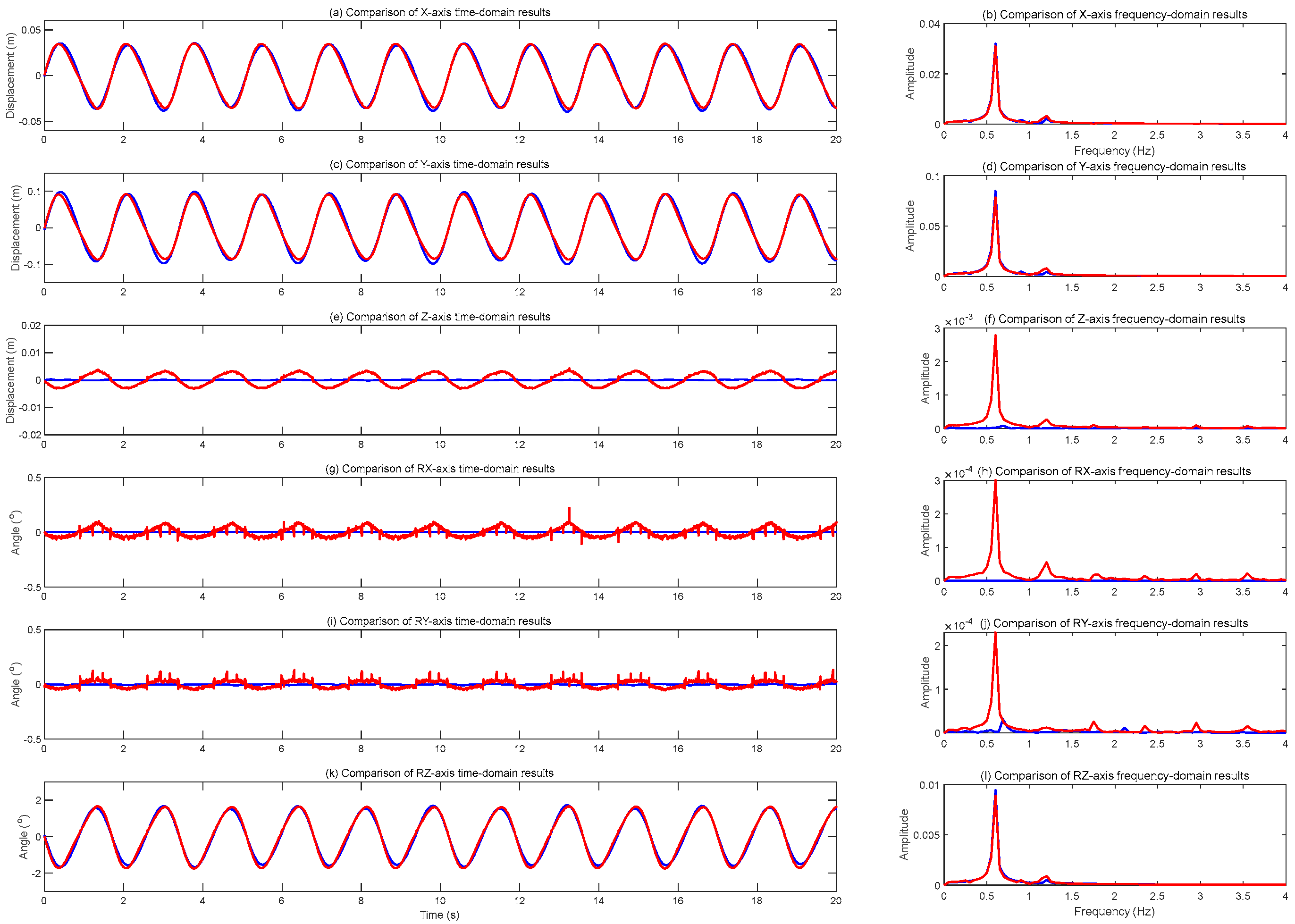
Figure 9a,c,e,g,i,k show the time-domain comparisons of the 6-DOF motions of the swing-arm buoy, where the red solid curves represent the results measured by the optical motion capture system (taken as the reference) and the blue solid curves denote the results computed by the proposed method. It can be observed that the two sets of measurements nearly coincided completely over the entire 20 s duration. The phase difference is less than 0.02 s, and the amplitude discrepancy exhibits only minor fluctuations at local peaks. In particular, in regions where the motion amplitude is large, the two curves almost overlap, yielding the highest identification accuracy. In transition phases where the displacement or rotation angle is very small, the measurement error increases slightly due to the limitations imposed by the camera pixel resolution and the system static noise, but it remains within an acceptable range for engineering applications. To quantitatively evaluate the measurement accuracy, the root mean square error (RMSE) and the normalized RMSE (NRMSE) were computed for the primary motion directions. The RMSE values for $X$, $Y$, and $RZ$ are 0.003159 cm, 0.009571 cm, and 0.139677°, respectively, while the corresponding NRMSE values are 4.43%, 5.34%, and 4.19%, confirming the high accuracy of the proposed method for the dominant motion components. To further assess the statistical reliability of the measurements, 95% confidence intervals were computed for the error sequences, yielding [−0.000320, 0.000183] cm, [−0.000483, 0.001039] cm, and [−0.019312, 0.002880]°, respectively. These results indicate that the proposed method can accurately capture both the transient motion characteristics and the steady-state response of the floating structures, with particularly outstanding performance in identifying significant motions. To further verify the measurement accuracy in the frequency domain, a frequency-domain analysis was performed on both sets of results, as shown in Figure 9b,d,f,h,j,l. The dominant frequency extracted by the proposed method is 0.59 Hz, which is in exact agreement with that obtained from the optical motion capture system. The dominant frequency errors in the $X$, $Y$, and $RZ$ directions are nearly zero, demonstrating the frequency-domain accuracy of the proposed method.

Figure 9. Comparison of time-domain and frequency-domain response results.

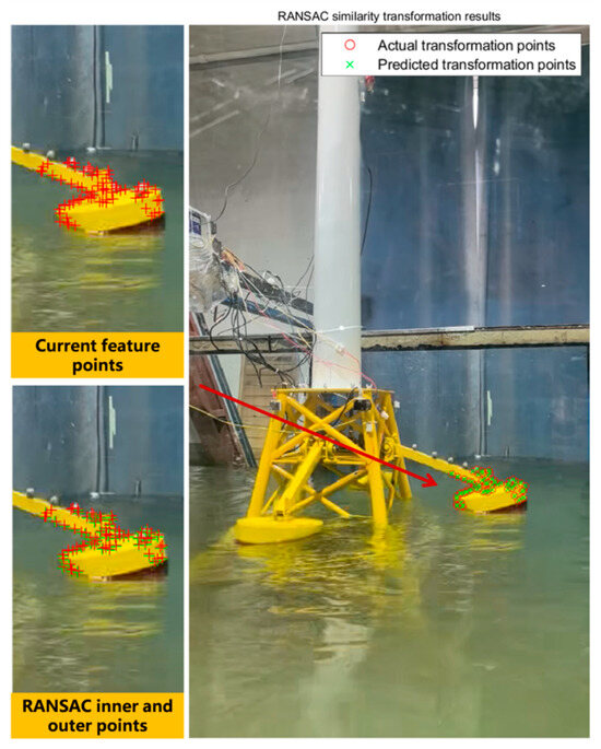
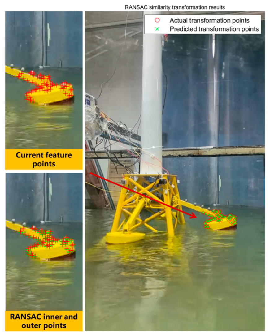
Figure 10 illustrates the RANSAC similarity transformation fitting performance at the 10th frame. The green crosses indicate the feature point positions predicted by the transformation model, while the red circles represent the actually tracked feature point positions. The two sets of markers are highly coincident, confirming that the similarity transformation model achieves satisfactory fitting accuracy. Inliers are marked by green “+” symbols and outliers by yellow “o” symbols; the two categories are clearly distinguished, which intuitively demonstrates the capability of the RANSAC algorithm to eliminate erroneous matches.

Figure 10. RANSAC similarity transformation fitting result.

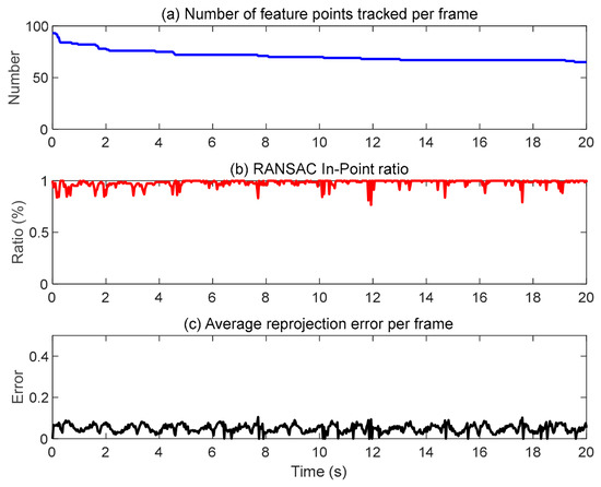
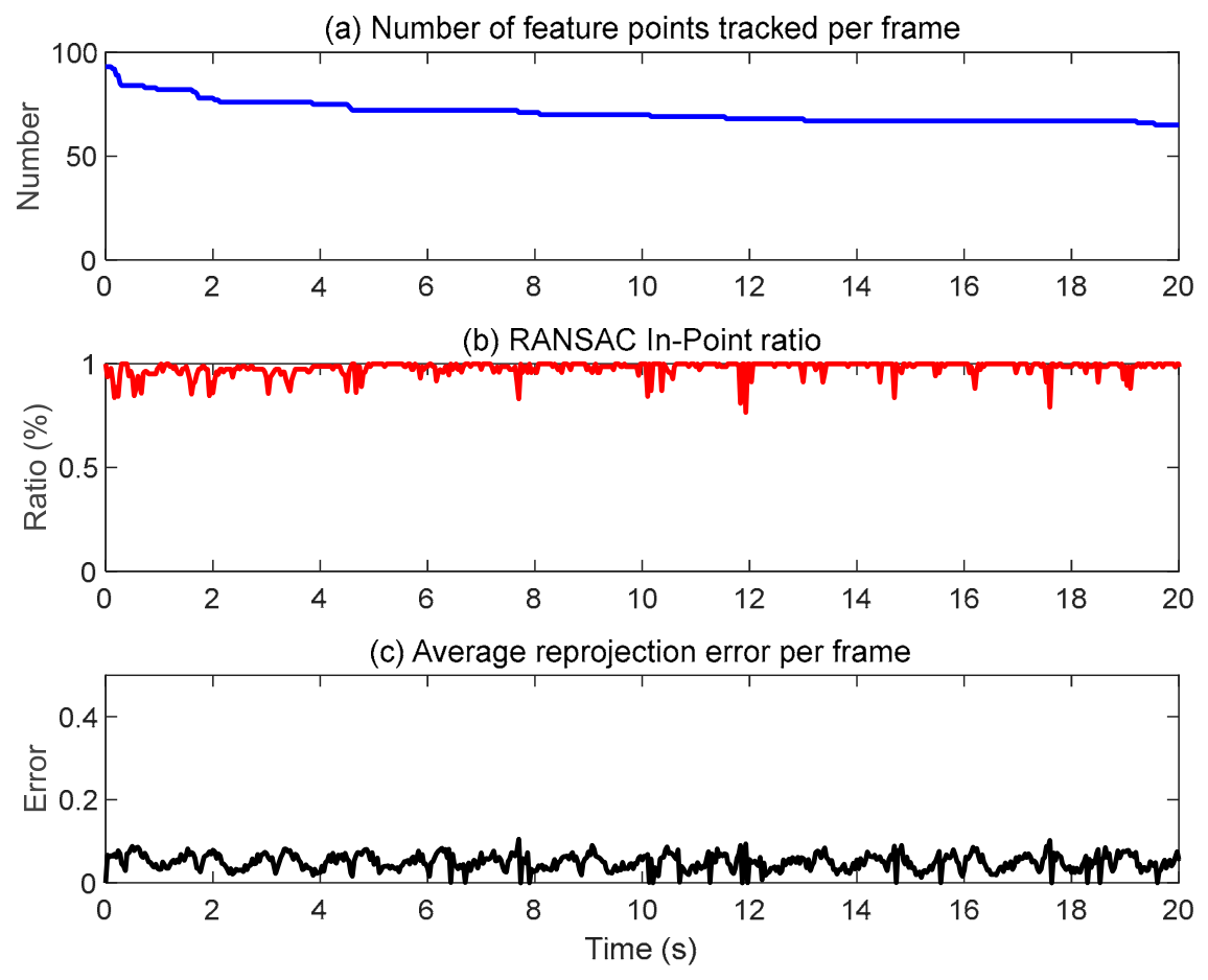
To quantitatively evaluate the quality of feature point tracking and the robustness of the system, Figure 11a–c present the time histories of three core tracking metrics under this test condition. The results show that the number of valid feature points remains consistently above 60, with a mean value of 74.97, which exceeds the minimum threshold of 20 and thus provides sufficient geometric redundancy for motion calculation. The RANSAC inlier ratio $r_{in}^k$ stays above 80% throughout the entire duration, reaches a peak of 100%, and yields an average of 92.98%, indicating that most of feature point matches satisfy the geometric consistency requirement of the similarity transformation. The root-mean-square reprojection error has a mean value of 0.0436 and exhibits a concentrated distribution, suggesting that the tracking accuracy is stable and reliable. These metrics demonstrate that the proposed method is capable of achieving long-term stable tracking of the natural textures on the floating structures surface, even in an experimental environment subject to specular water-surface reflections and wave spray interference. The computational efficiency of the proposed method was evaluated on a standard desktop computer (Intel Core i7-14700) running MATLAB R2024b. The average processing time was approximately 0.04 s per frame, corresponding to a processing rate of approximately 25 Hz, which is sufficient for offline analysis of the experimental data.

Figure 11. Temporal evolution of tracking quality metrics.

4.3. Influence of Measurement Distance on Accuracy

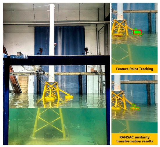
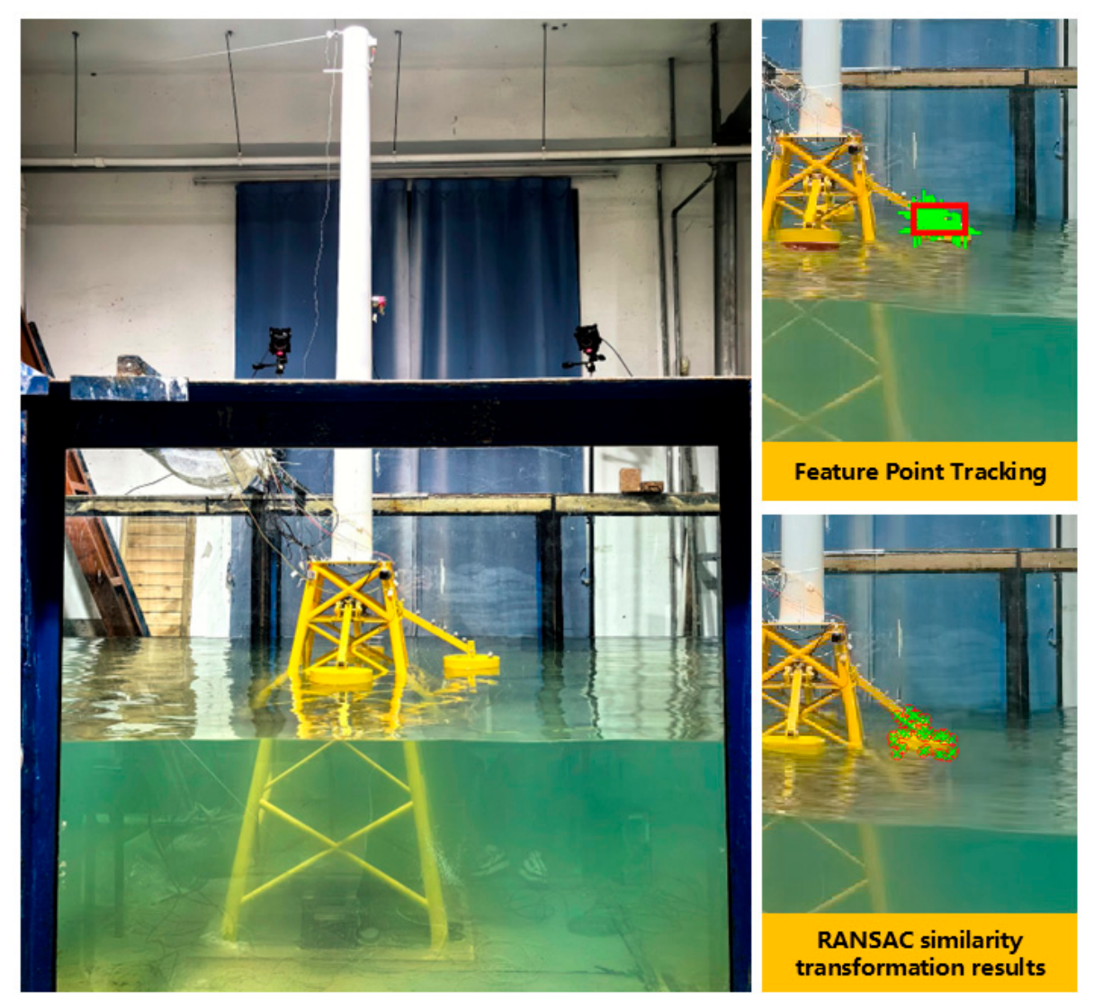
To investigate the influence of the camera-to-buoy observation distance on measurement accuracy and to verify the adaptability of the method under different field deployment conditions, a repeated comparative test was conducted at a straight-line distance of 3.5 m under the same wave condition, with the buoy motion state, camera parameters, and illumination conditions kept entirely consistent. Figure 12 shows the on-site experimental arrangement, the feature point tracking, and the RANSAC similarity transformation fitting results during the system analysis. Table 2 summarizes the comparison of three primary metrics—the number of valid feature points, the RANSAC inlier ratio, and the root-mean-square reprojection error—between the two distances.

Figure 12. Feature point tracking and RANSAC fitting results at an observation distance of 3.5 m.

Table 2. Comparison of errors at different distances.

		1.6 m	3.5 m
Number of valid feature points	Mean	74.9652	70.7853
	Minimum	65	52
Inlier ratio (%)	Mean	92.98	88.351
	Maximum	100	100
	Minimum	0.8047	0.7921
Reprojection error	Mean	0.0436	0.0404
NRMSE (%)	$X$$,Y$$,RZ$	4.43, 5.34, 4.19	4.64, 6.62, 4.99
Frequency-domain results (Hz)	$X$$,Y$$,RZ$	0.59	0.59

The comparison results indicate that, even when the observation distance is more than doubled, the measurement accuracy at the two distances remains essentially identical, with no significant degradation. These results confirm that the method developed in this study exhibits strong robustness to image scale variations within the tested range (1.6 m to 3.5 m), maintains stable measurement accuracy over a wide range of observation distances, and offers considerable flexibility for on-site deployment.

5. Validation Through Physical Model Tests in the Wave Tank

In Section 4, the correctness of the developed method was preliminarily validated through physical model tests using regular waves. However, waves in actual marine environments are irregular and inherently stochastic, and field monitoring is further challenged by complex interfering factors such as uneven illumination, water surface reflections, and wave spray, none of which can be fully reproduced by a single regular wave test. To further demonstrate the feasibility and robustness of the proposed method under realistic marine conditions, physical model tests of JONSWAP-spectrum irregular waves were conducted in the wave tank at the Shandong Provincial Key Laboratory of Ocean Engineering, Ocean University of China. The measurement accuracy, tracking stability, and adaptability to different observation distances of the proposed method under irregular wave action were systematically evaluated.

5.1. Wave Tank Experimental Setup

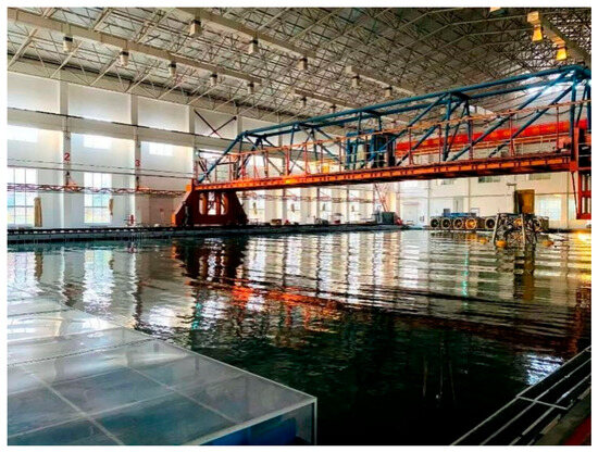
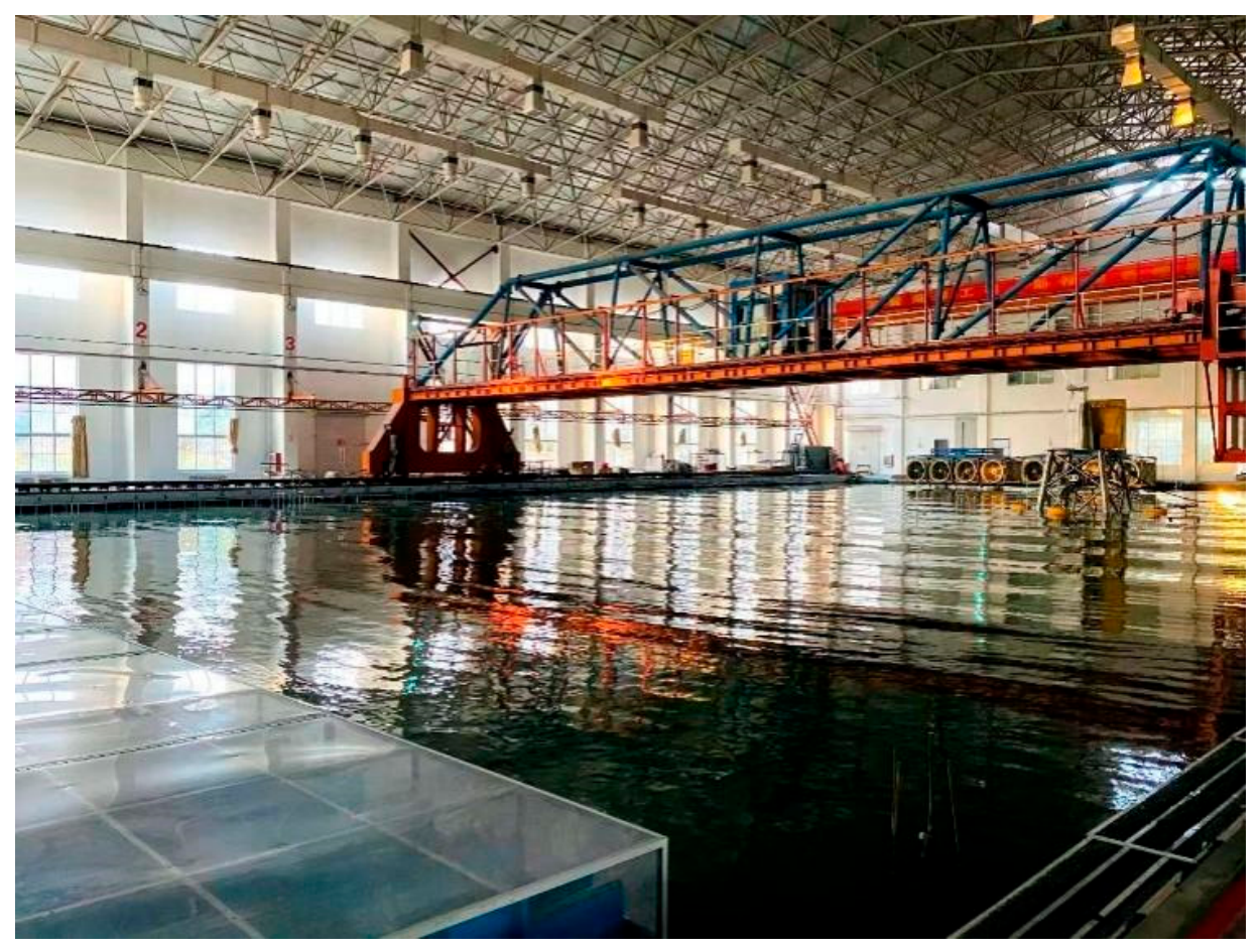
The experiments in this section were performed in the wave tank at Ocean University of China, as illustrated in Figure 13. The tank is 60 m long, 36 m wide, and has a maximum water depth of 1.5 m. Three piston-type wave makers are installed at the front end, capable of generating both regular waves and JONSWAP-spectrum irregular waves. The significant wave height ranges from 0.03 m to 0.25 m, and the spectral peak period ranges from 0.5 s to 3 s. Wave-absorbing nets are uniformly arranged at the rear end and along both sides of the tank to damp reflected waves.

Figure 13. Wave tank.

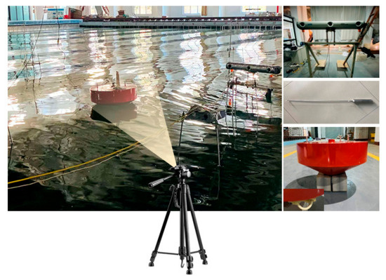
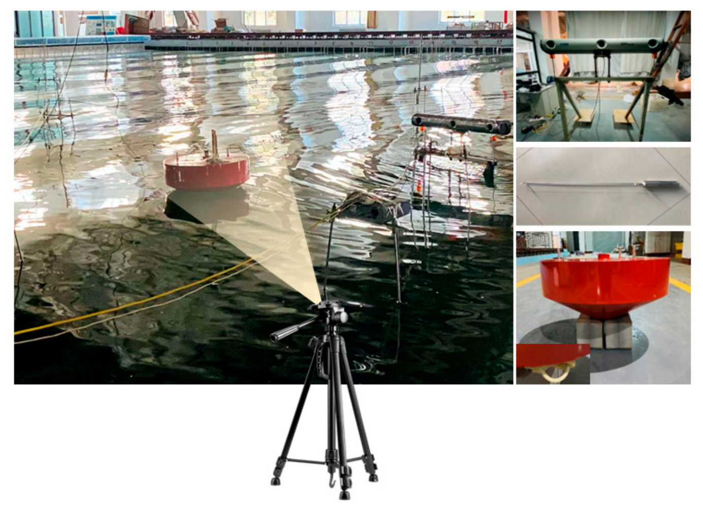
The experimental model was an oscillating buoy, designed according to the Froude similarity criterion at a scale ratio of $\lambda =8$. The buoy body was made of aluminum alloy and featured a cylindrical–conical combined shape, with a conical bottom intended to reduce wave impact during heave motion. The model had a draft of 0.233 m and a total mass of 11.164 kg. The upper cylindrical section of the buoy was 0.1875 m high, the lower conical section was 0.2165 m high, and the cone angle was 120°. To prevent excessive horizontal drift of the buoy under wave action, which would cause it to move outside the camera’s field of view, a flexible rope was attached with a clip at the waterline height, and the other end of the rope was fixed to the side wall of the tank, thereby imposing only a flexible constraint on the horizontal motion of the buoy. In this experiment, the $X$-axis of the world coordinate system was defined along the wave propagation direction, the $Y$-axis vertically upward, and the $Z$-axis according to the right-hand rule. The experimental setup is illustrated in Figure 14.

Figure 14. Wave tank experimental setup.

The primary measurement instruments included the following: (1) An NDI Optotrak Certus 6-DOF measurement system (Northern Digital Inc., Canada). This system employed three high-resolution, high-speed infrared linear-array cameras to capture infrared markers attached to the upper surface of the buoy, enabling real-time monitoring of the motion response of the oscillating buoy. The sampling frequency of the system was set to 50 Hz. (2) Capacitance wave gauges (China). An SG2000 data acquisition instrument together with capacitance wave gauges was used to monitor the waves in real time, in order to verify the accuracy of the wave height generated by the wave-making system. (3) A monocular camera with a resolution of 1920 × 1080 pixels and a frame rate of 30 fps (China). The camera was fixedly mounted on one side of the tank, with its optical axis aligned with the center of the buoy’s motion range, and was used to acquire continuous image sequences of the buoy motion.

5.2. Measurement Accuracy Verification

An irregular wave case with a significant wave height of 0.08 m and a peak period of 1.7 s was selected for dynamic response identification. Under the scale ratio of 1:8, this condition corresponds to a typical operational sea state for the target application site—the coastal waters of northern China—to validate the method’s performance under realistic operational conditions. The camera was positioned at a straight-line distance of 4 m from the buoy. After the buoy motion reached a steady periodic state under wave excitation, a 30 s video was continuously recorded, and reference data from the NOKOV optical motion capture system were synchronously acquired for accuracy comparison.

When processing the initial frame, a polygonal ROI covering the buoy body was first defined to isolate interference from water surface waves and the background shoreline. The vertex coordinates of this ROI were then used to generate a binary mask, which confined all subsequent feature point detection and tracking operations within the mask. Figure 15 illustrates the ROI initialization process, showing that the mask accurately encloses the buoy region and effectively excludes background interference.

Figure 15. Polygonal ROI and image initialization.

Figure 16 compares the output of three detectors—Minimum Eigenvalue, SURF, and FAST—within the same ROI. The Minimum Eigenvalue corner detector (Figure 16a) yielded 158 feature points, which exhibited the most uniform distribution and are concentrated in texture-rich regions. In contrast, the SURF detector (Figure 16b) and the FAST detector (Figure 16c) detected 21 and 17 feature points, respectively, both with pronounced local clustering. Considering the need for an even spatial distribution of feature points in the subsequent tracking stage, the Minimum Eigenvalue corners were adopted as the initial feature point set. If the number of detected points fell below a minimum threshold of 20, the SURF and FAST algorithms are sequentially activated as supplementary sources.

Figure 16. Comparison of feature point detection results among Minimum Eigenvalue, SURF, and FAST.

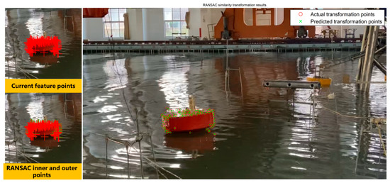
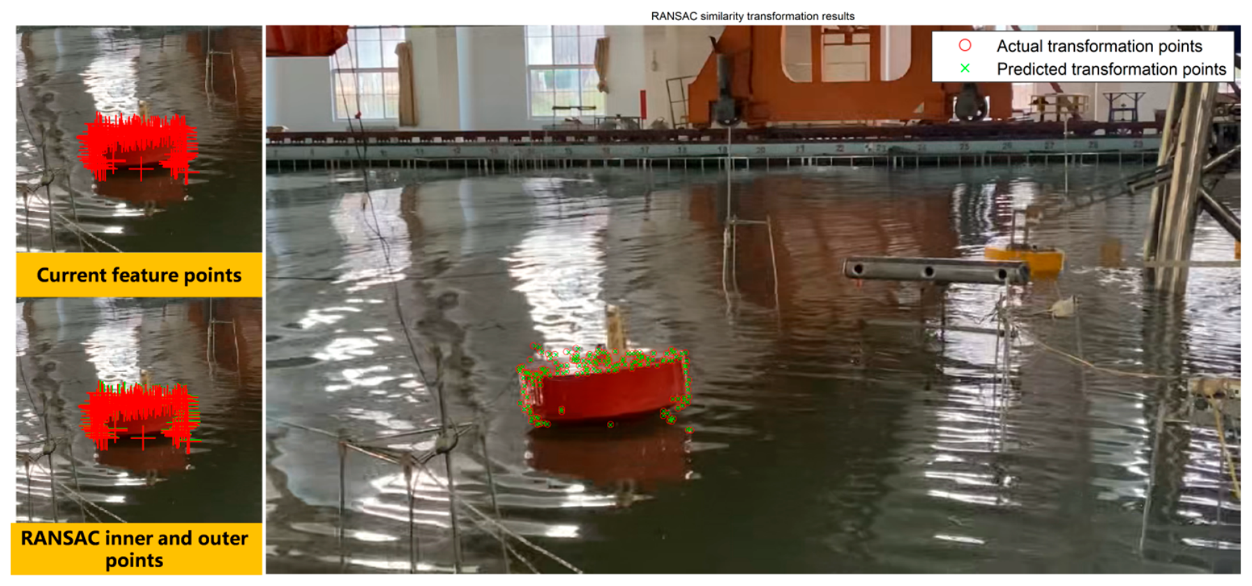
A pyramidal KLT optical flow algorithm was employed to realize inter-frame feature point tracking. By decomposing large displacement motion into multiple levels of small displacements and solving them progressively using an image pyramid, tracking failure induced by fast buoy motion was avoided. To eliminate mismatches, forward–backward bidirectional verification was first applied to remove erroneous correspondences caused by occlusion and illumination variations. Subsequently, the RANSAC algorithm was used to fit a similarity transformation model, which further discarded outliers arising from water surface reflections, motion blur, and similar effects. Figure 17 illustrates the RANSAC fitting result for frame 172. The green cross marks represent model-predicted points, and the red dots indicate the actual tracked points. Their close overlap demonstrates the high accuracy of the similarity transformation fit. The green plus signs mark inliers, whereas the yellow circles indicate outliers, thereby clearly distinguishing correct matches from erroneous ones. The detailed identification process is shown in Figure 18.

Figure 17. RANSAC similarity transformation fitting results.

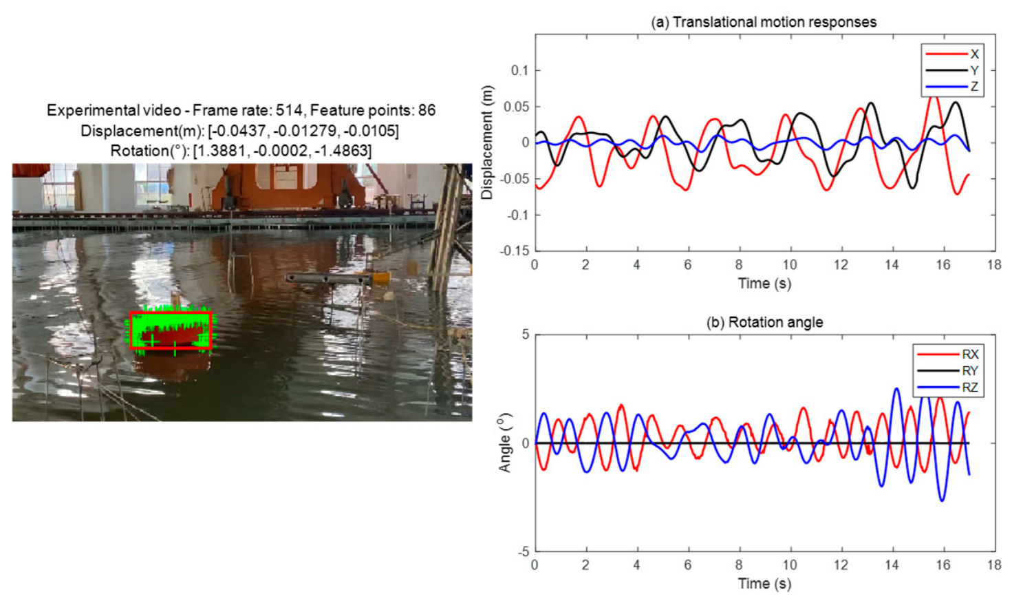
Figure 18. Identification of buoy 6-DOF motion.

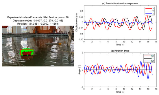
Figure 19 compares the time-domain curves of the buoy 6-DOF motion measured by the proposed method and the NDI system. Over the 30 s irregular wave duration, the overall trends of the two sets of curves are highly consistent, with a phase difference of less than 0.1 s. Specifically, for the $X$ and $Y$ directions, which are the primary degrees of freedom of the buoy in head waves, the curves nearly coincide perfectly; the time-domain responses of $RX$ and $RZ$ also agree well with the reference results. In contrast, the $Z$ and $RY$ motions could not be fully identified due to their extremely small amplitudes, and the measurement errors increased slightly. To quantitatively evaluate the measurement accuracy under irregular wave conditions, the RMSE and the NRMSE were computed for the primary motion directions. The RMSE values for $X$, $Y$, $RX$, and $RZ$ are 0.023333 cm, 0.014022 cm, 0.548991°, and 0.848676°, respectively, while the corresponding NRMSE values are 8.17%, 7.80%, 7.98%, and 9.68%, further confirming the effectiveness of the proposed method. To further assess the statistical reliability of the measurements, 95% confidence intervals were computed for the error sequences, yielding [−0.016223, 0.012923] cm, [−0.001351, 0.001188] cm, [−0.204627, 0.293234]°, and [−0.025072, 0.177655]°, respectively, all of which contain zero, indicating the absence of systematic bias. The RMSE values and confidence intervals collectively demonstrate that the proposed method maintains consistent measurement accuracy across all four degrees of freedom under irregular wave conditions. These results indicate that the proposed method achieves higher identification accuracy for large-amplitude motions and can effectively capture the main motion characteristics of the buoy under irregular wave excitation. To further evaluate the measurement accuracy, frequency-domain analysis was performed on both sets of motion data. The results show that the dominant first-order motion frequency for $X$, $Y$, and $RZ$ is 0.367 Hz, which is fully consistent with that obtained by the reference system, with a dominant frequency error essentially zero. For $Z$, $RX$, and $RY$, owing to their low motion amplitudes, the amplitude errors of higher-order harmonic components increased. Compared with the regular wave tank test results presented in Section 4, the motion identification accuracy in this test decreased slightly. This degradation was mainly attributable to the fact that the wave tank test environment is closer to actual marine conditions: the larger tank space led to uneven illumination distribution, the large water surface caused more extensive specular reflection interference, and the spray interference induced by the JONSWAP-spectrum irregular waves exhibited greater randomness and persistence. Despite these challenging conditions, which were designed to emulate real-world marine environments, the proposed method still accurately reproduced the time-domain and frequency-domain characteristics of the buoy’s main degrees of freedom, demonstrating that even under more complex simulated marine conditions, the method achieved long-term stable tracking of the natural texture on the buoy surface, without tracking loss or a sudden drop in accuracy.

Figure 19. Comparison of time-domain and frequency-domain response results.

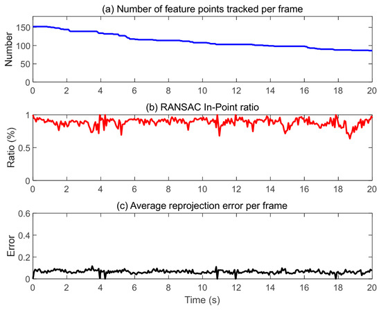
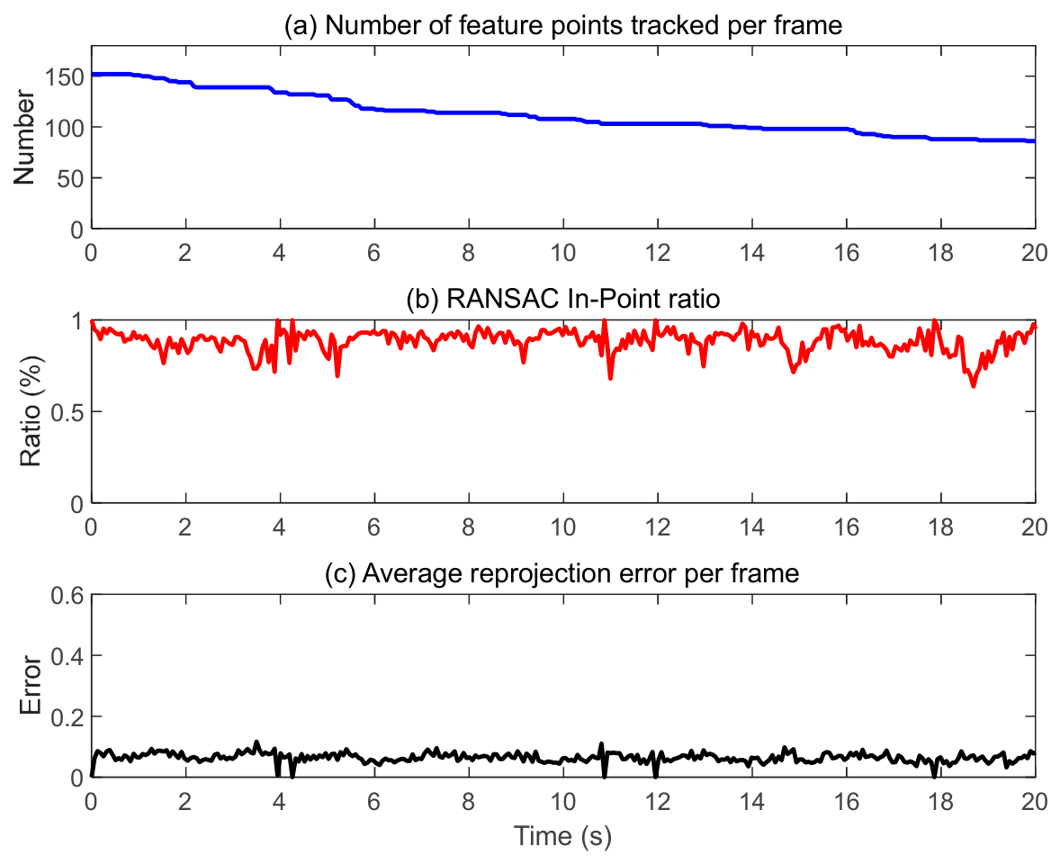
Three core metrics—namely, the number of effective feature points, the RANSAC inlier ratio, and the reprojection error—were employed to quantitatively evaluate the tracking quality and robustness of the proposed method under irregular wave conditions, as shown in Figure 20. The statistical results show that the number of effective feature points consistently remained above 60, with an average of 101.68, which far exceeded the minimum threshold of 20, thus providing sufficient geometric redundancy for motion estimation. The RANSAC inlier ratio remained above 75%, reached a peak of 99%, and averaged 85.23%, indicating that most of feature point matches satisfied the geometric consistency requirement of the similarity transformation. The mean reprojection error was 0.0604, and the error distribution was concentrated, exhibiting no abrupt changes.

Figure 20. Temporal evolution of tracking quality metrics.

6. Summary and Conclusions

This paper presents a monocular vision-based feature point tracking method for measuring the 6-DOF motion of marine floating structures. The method exploits the natural texture on the floating structures surface and performs feature tracking through a multi-strategy cascaded detection approach combining Minimum Eigenvalue, SURF, and FAST, integrated with pyramidal KLT optical flow. After geometric consistency verification using RANSAC, the in-plane translation and $RZ$ angles are extracted from the similarity transformation. The $RX$ and $RY$ angles are estimated from the variations in the principal orientation angle and aspect ratio via principal component analysis of the covariance matrix of the feature point set, while the displacement in the depth direction is obtained by linearly mapping the change in the scale factor. The entire method requires only a single camera and eliminates the need for inertial sensors and artificial cooperative targets.

Physical model tests were conducted in a wave flume and a wave tank, respectively, using a jacket-type combined wind–wave energy converter and an oscillating buoy as test objects. Comparisons were performed against a high-precision optical motion capture system to validate the accuracy and engineering applicability of the proposed method in this paper. The static stability test results demonstrate that the proposed method exhibits excellent static measurement accuracy and robustness against ambient environmental noise. Under both regular wave and JONSWAP spectrum irregular wave conditions, the NRMSE values for the primary motion directions are all below 10%, and the dominant frequency identification errors for large-amplitude motion directions are essentially zero. During the tracking process, the inlier ratio of RANSAC geometric consistency verification is consistently maintained above 80%, and the mean reprojection error is less than 0.05, achieving long-term stable tracking of natural texture feature points on the floating structure surface. Comparative tests at different observation distances further confirm that the proposed method has strong robustness to image scale variations, maintains stable measurement accuracy over a wide observation range, and possesses favorable on-site deployment flexibility. Comprehensive experimental results indicate that the proposed monocular vision measurement method, which requires no artificial cooperative targets or auxiliary inertial sensors, can realize high-precision non-contact measurement of 6-DOF motions of marine floating structures. It demonstrates significant advantages in terms of low cost, easy deployment, and robustness, as validated under both regular and irregular wave conditions in two independent physical model tests, thereby providing reliable technical support for the on-site condition monitoring of marine floating structures.

In future work, we will incorporate a deep feature point detection network to enhance tracking capability in texture-poor scenes. We also plan to extend the current framework to a multi-modal task by integrating complementary sensors such as IMUs with the monocular vision system to further improve robustness and generalization under varying sea conditions. In addition, a systematic sensitivity analysis of the calibration coefficients will be carried out to evaluate their impact on measurement accuracy.

References

- Shyamala, G.; Ravindran, G.; Alaneme, G.U.; Ramesh, T.; Dhanapalan, S. Harnessing the future of renewable energy: Integrated insights of ocean energy. Energy Nexus 2026, 21, 100622. [Google Scholar] [CrossRef] [Scilit]
- Jiang, C.Y.; Cao, F.F.; Wang, Q.; Shi, H. Analysis method of WEC sub-system for hybrid wind-wave energy system based on reconstructed displacements. Ocean Eng. 2023, 278, 114268. [Google Scholar] [CrossRef] [Scilit]
- Huang, P.; Yu, Y.H. Integrated turbine and cable layout optimization for floating offshore wind farms: A techno-economic assessment. Energy Convers. Manag. X 2026, 31, 101955. [Google Scholar] [CrossRef] [Scilit]
- Chen, Y.; Yuan, L.H.; Qin, L.C.; Zhang, N.; Li, L.; Wu, K.; Zhou, Z. A forecasting model with hybrid bidirectional long short-term memory for mooring line responses of semi-submersible offshore platforms. Appl. Ocean Res. 2024, 105, 104145. [Google Scholar] [CrossRef] [Scilit]
- Delbeke, O.; Bastianel, G.; Yurtseven, K.; Ergun, H.; Moschner, J.D.; Driesen, J. Hybrid offshore solar-wind farms: The potential of integrating floating photovoltaics with offshore wind. Appl. Energy 2026, 410, 127486. [Google Scholar] [CrossRef] [Scilit]
- Lu, H.C.; Chang, S.; Chen, C.H.; Fan, T.; Chen, J. Replacement of force-to-motion relationship with state–space model for dynamic response analysis of floating offshore structures. Appl. Ocean Res. 2022, 119, 102977. [Google Scholar] [CrossRef] [Scilit]
- Gao, S.J.; Liu, F.S. Research on non-stationary characteristic test and decomposition for dynamic response of floating structures. Ocean Eng. 2024, 292, 116550. [Google Scholar] [CrossRef] [Scilit]
- Li, Y.; Feng, Y.T.; Liu, Y.L.; Wang, B.; Li, G.; Su, O.; Cui, Y.; Li, H. Dynamic response of upper structures on 15 MW floating offshore wind turbine after mooring line failure. Ocean Eng. 2025, 342, 123025. [Google Scholar] [CrossRef] [Scilit]
- Ambarita, E.E.; Karlsen, A.; Osen, O.; Hasan, A. Towards fully autonomous floating offshore wind farm operation & maintenance. Energy Rep. 2023, 9, 103–108. [Google Scholar] [CrossRef] [Scilit]
- Gao, X.G.; Jiang, J.Y.; Xu, G.Y.; Chang, Z.; Yang, J. Multi-antenna GNSS–accelerometer fusion attitude correction algorithm for offshore floating platform displacement monitoring. Sensors 2024, 24, 7804. [Google Scholar] [CrossRef] [Scilit] [PubMed]
- Mu, X.K.; He, B.; Wu, S.Y.; Zhang, X.; Song, Y.; Yan, T. A practical INS/GPS/DVL/PS integrated navigation algorithm and its application on Autonomous Underwater Vehicle. Appl. Ocean Res. 2021, 106, 102441. [Google Scholar] [CrossRef] [Scilit]
- Zhu, H.; Zhou, Y.J.; Hu, Y.M. Displacement reconstruction from measured accelerations and accuracy control of integration based on a low-frequency attenuation algorithm. Soil Dyn. Earthq. Eng. 2020, 133, 106122. [Google Scholar] [CrossRef] [Scilit]
- Liu, F.S.; Gao, S.J.; Liu, Y.; Liu, D. A motion tracking approach to position marine floating structures based on measured acceleration and angular velocity. Ocean Eng. 2022, 257, 111682. [Google Scholar] [CrossRef] [Scilit]
- Jiang, Y.; Guo, C.; Wang, J.; Xu, R. Multipath effects mitigation in offshore construction platform GNSS-RTK displacement monitoring using parametric temporal convolution network. Remote Sens. 2025, 17, 601. [Google Scholar] [CrossRef] [Scilit]
- Chen, H.B.; Moan, T.; Verhoeven, H. Effect of DGPS failures on dynamic positioning of mobile drilling units in the North Sea. Accid. Anal. Prev. 2009, 41, 1164–1171. [Google Scholar] [CrossRef] [Scilit] [PubMed]
- Dong, Y.H.; Din, M.U.; Lagala, F.; Kuang, H.; Sun, J.; Yang, S.; Hussain, I.; He, S. Drone carrier: An integrated unmanned surface vehicle for autonomous inspection and intervention in GNSS-denied maritime environment. J. Ocean Eng. Sci. 2026; in press. [CrossRef] [Scilit]
- Leng, J.C.; Ma, J.Y.; Feng, H.Y. An adaptive convolutional neural network based on transmissibility grayscale image for online identification of offshore platform damage pattern. Mech. Syst. Signal Process. 2024, 221, 111713. [Google Scholar] [CrossRef] [Scilit]
- Qi, Q.H.; Xu, X.W.; Deng, M.X.; Guo, X.; Ma, J. A vision-based object detection approach for tugboat escort and its application in a camera pan-tilt control system. Ocean Eng. 2025, 334, 121540. [Google Scholar] [CrossRef] [Scilit]
- Xu, W.L.; Liang, C.; Lian, J.J.; Wang, J.; Yao, Y. Experimental validation of robust stereo-vision-based 6-DOF motion measurement for offshore floating photovoltaic platforms. Sol. Energy 2026, 314, 114673. [Google Scholar] [CrossRef] [Scilit]
- Liang, H.Q.; Lu, Y.J.; Chen, H.R.; Zhang, Z.; Guo, T.; Shen, S.; Zhi, G. Vision-based measurement of TLCD/TLCGD dynamic performance with application to offshore wind turbine shaking table tests. Structures 2026, 89, 111975. [Google Scholar] [CrossRef] [Scilit]
- Wang, R.Z.; Tian, X.L.; Fang, X.K.; Guo, X.; Lu, W.; Wang, P.; Li, X.; Yuan, M. Mage recognition-based high-precision 6DOFs motion capture method for large floating vessels during float-over operations. Ocean Eng. 2025, 337, 121801. [Google Scholar] [CrossRef] [Scilit]
- Yi, J.H.; Kim, J.H.; Jeong, W.M.; Chae, J.-W. Field evaluation of optical-based three-dimensional dynamic motion measurement system with multiple targets for a floating structure. Ocean Eng. 2013, 62, 140–151. [Google Scholar] [CrossRef] [Scilit]
- Guo, L.J.; Guo, W.H.; Chen, D.S.; Shi, Z.; Tan, M. Large displacement measurement using deep learning-based RAFT and KLT optical flow. Mech. Syst. Signal Process. 2025, 241, 113538. [Google Scholar] [CrossRef] [Scilit]
- Cai, Z.Y.; Huang, Y.W.; Zhang, T.F.; Zheng, Y.; Yue, D. Multi-Source Domain Adaptation by Causal-Guided Adaptive Multimodal Diffusion Networks. Int. J. Comput. Vis. 2025, 133, 4623–4645. [Google Scholar] [CrossRef] [Scilit]
- Kang, B.S.; Jung, C.H. Detecting Maritime Obstacles Using Camera Images. J. Mar. Sci. Eng. 2022, 10, 1528. [Google Scholar] [CrossRef] [Scilit]
- Basecetta, L.; Ferretti, G.; Rocco, P.; Ardö, H.; Bruyninckx, H.; Demeester, E.; Di Lello, E. Towards safe human-robot interaction in robotic cells: An approach based on visual tracking and intention estimation. In Proceedings of the 2011 IEEE/RSJ International Conference on Intelligent Robots and Systems, San Francisco, CA, USA, 25–30 September 2011. [Google Scholar]
- Jeon, G.; Kim, S.; Ahn, S.; Kim, H.; Yoon, H. Vision-based automatic cable displacement measurement using Cable-ROI Net and Uni-KLT. Struct. Control Health Monit. 2022, 29, e2977. [Google Scholar] [CrossRef] [Scilit]
- Nguyen, X.T.; Jeon, G.; Vy, V.; Lee, G.; Lam, P.T.; Yoon, H. A hybrid approach for vision-based structural displacement measurement using transforming model prediction and KLT. Mech. Syst. Signal Process. 2025, 223, 111866. [Google Scholar] [CrossRef] [Scilit]
- Xia, S.J.; Qin, R.F.; Lu, Y.; Ma, L.; Liu, Z. A Monocular Vision-Based Safety Monitoring Framework for Offshore Infrastructures Utilizing Grounded SAM. J. Mar. Sci. Eng. 2025, 13, 340. [Google Scholar] [CrossRef] [Scilit]
- Zhou, G.Q.; Tang, Y.; Xie, Y.F.; Song, R.; Zhu, Q.; Zhou, X. Calibration of Fisheye Camera With Colinear Constraint of the Main Optical Axis and Epipolar Line Orthogonality-Transverse Axis. IEEE Sens. J. 2024, 24, 19373–19384. [Google Scholar] [CrossRef] [Scilit]
- Zhuang, Y.H.; Chen, W.M.; Jin, T.; Chen, B.; Zhang, H.; Zhang, W. A Review of Computer Vision-Based Structural Deformation Monitoring in Field Environments. Sensors 2022, 22, 3789. [Google Scholar] [CrossRef] [Scilit] [PubMed]
- Rebeish, F.A.; Shageer, H.; Sayed, M.A. AI-Powered Monocular Perception for Collision Avoidance and Resilient Navigation in Unmanned Surface Vessels. Transp. Res. Procedia 2026, 96, 292–299. [Google Scholar] [CrossRef] [Scilit]
- Sun, C.B.; He, W.; Zou, C. High-Precision Visual Monitoring Method for Bridge Displacement Based on Computer Vision and Its Engineering Application. Appl. Sci. 2025, 15, 10023. [Google Scholar] [CrossRef] [Scilit]
- Shi, J.; Tomasi, C. Good features to track. In Proceedings of the 1994 IEEE Conference on Computer Vision and Pattern Recognition, Seattle, WA, USA, 21–23 June 1994; pp. 593–600. [Google Scholar]
- Bay, H.; Tuytelaars, T.; Van Gool, L. SURF: Speeded up robust features. In Computer Vision—ECCV 2006, Proceedings of the 9th European Conference on Computer Vision, Graz, Austria, 7–13 May 2006, Proceedings, Part I; Springer: Berlin/Heidelberg, Germany, 2006; pp. 404–417. [Google Scholar]
- Rosten, E.; Drummond, T. Machine learning for high-speed corner detection. In Computer Vision—ECCV 2006, Proceedings of the 9th European Conference on Computer Vision, Graz, Austria, 7–13 May 2006, Proceedings, Part I; Springer: Berlin/Heidelberg, Germany, 2006; pp. 430–443. [Google Scholar]
- Ma, S.H.; Guo, P.K.; You, H.R.; He, P.; Li, G.; Li, H. An image matching optimization algorithm based on pixel shift clustering RANSAC. Inf. Sci. 2021, 562, 452–474. [Google Scholar] [CrossRef] [Scilit]
Disclaimer/Publisher’s Note: The statements, opinions and data contained in all publications are solely those of the individual author(s) and contributor(s) and not of MDPI and/or the editor(s). MDPI and/or the editor(s) disclaim responsibility for any injury to people or property resulting from any ideas, methods, instructions or products referred to in the content. |
© 2026 by the authors. Licensee MDPI, Basel, Switzerland. This article is an open access article distributed under the terms and conditions of the Creative Commons Attribution (CC BY) license.