


Abstract
Bilevel optimization problems (BOPs) are widely encountered in hierarchical decision-making, wherein the embedding of the lower-level problem within the upper-level problem poses significant challenges to the solution process. To solve complex BOPs, this paper proposes a coordinated feedback-based hierarchical triangulation topology aggregation optimizer (CFHTTAO). CFHTTAO is developed by constructing a hierarchical solution framework and designing improvement mechanisms to enhance its performance. Specifically, a knowledge-sharing mechanism is established to promote information exchange among triangular topological units, a coordinated feedback mechanism is designed to adaptively select a suitable lower-level search method and feed the obtained lower-level solution back to the upper level, and an elite learning evolution mechanism is used to reduce the risk of premature convergence. CFHTTAO is evaluated on the SMD test suite under different dimensional settings, where the test problems involve various complex characteristics of BOPs. In addition, the Friedman test results show that CFHTTAO achieves the smallest mean ranks, with upper-level mean ranks of 1.08, 1.50, and 1.50 and lower-level mean ranks of 1.00, 1.17, and 1.25 on the SMD, SMD, and SMD problems, respectively. Finally, CFHTTAO is applied to the inverse optimal control problem as the practical case study. Overall, experimental results demonstrate that CFHTTAO achieves better solution accuracy, stronger stability, and faster convergence when solving complex BOPs, and exhibits strong applicability to the practical bilevel optimization task.
Keywords:
bilevel optimization; triangulation topology aggregation optimizer; hierarchical framework; coordinated feedback MSC:
90C26; 90C59
1. Introduction
Many practical problems involve hierarchical decision-making structures, in which decisions at one level influence decisions at the other level [1,2]. These problems are formulated as bilevel optimization problems (BOPs) and arise in various applications [3], such as supply chain management [4], renewable energy communities [5], and inverse optimal control [6]. Solving linear BOPs has been proven to be NP-hard, and the solution difficulty is further intensified when BOPs involve complex characteristics such as nonlinearity, nonconvexity, and multimodality, which often limit the applicability of traditional methods [7]. Therefore, it is of great importance to explore more effective algorithms for BOPs, as this can advance methodological developments in bilevel optimization and promote its practical applications.
A bilevel optimization problem consists of an upper-level problem and a lower-level problem, where the lower-level problem is embedded within the upper-level problem. To address the nested structure of BOPs, existing studies can be classified into two main categories: single-level reduction methods and nested methods. Among them, single-level reduction methods transform the bilevel optimization problem into a single-level formulation [8]. However, single-level reduction methods typically rely on specific properties of the problem. When the lower-level problem is nonconvex or fails to satisfy sufficient regularity conditions, deriving an equivalent single-level reformulation becomes difficult, which limits the applicability of single-level reduction methods to complex BOPs [7,9]. Compared with single-level reduction methods, nested methods can preserve the original structure of BOPs and avoid the dependence on specific function properties typically required by single-level reduction methods, which gives nested methods broader applicability to complex BOPs [10]. By embedding the lower-level solution process into the upper-level process, nested methods have been widely applied [7,11]. In recent years, combining nested methods with intelligent optimization algorithms has gradually become an important direction for solving complex BOPs [12,13]. Meanwhile, with the development of artificial intelligence, new intelligent optimization algorithms have continuously emerged. These include triangulation topology aggregation optimizer (TTAO), a new optimization algorithm [14]. Owing to its simple parameter setting and practical applicability, TTAO has attracted increasing attention and shown potential for solving complex optimization problems [15,16].
Solving BOPs is inherently challenging, as even linear BOPs have been proven to be NP-hard [17,18]. In the real world, these problems usually involve more complex characteristics, such as nonlinearity, nonconvexity, and high dimensionality, which further aggravate the solution difficulty. Nevertheless, effective algorithms designed for complex BOPs remain relatively insufficient. Therefore, CFHTTAO is proposed to solve complex BOPs. CFHTTAO is based on TTAO and integrates the nested hierarchical solution framework with the designed improvement mechanisms to enhance its performance. Furthermore, SMD problems under different dimensional settings are used to evaluate the effectiveness of CFHTTAO, as these problems involve various complex characteristics of BOPs. CFHTTAO is compared with other algorithms developed for solving BOPs, and its effectiveness is further verified through the practical application. The key contributions of this paper are as follows.
- (1)
- A novel hierarchical coordinated method with triangular topological structures is proposed for solving BOPs. It reorganizes information exchange among triangular topological units, constructs a new coordinated feedback method for the lower level, and establishes differentiated methods tailored to the tasks at the upper and lower levels.
- (2)
- CFHTTAO is proposed to solve complex BOPs. CFHTTAO adopts a nested hierarchical solution framework and avoids the strict reformulation requirements. It shows broader applicability to complex BOPs involving challenging characteristics such as nonlinearity and nonconvexity.
- (3)
- A knowledge-sharing mechanism is designed to enhance information exchange among triangular topological units. By constructing a knowledge pool, this mechanism strengthens information communication among different units and helps the algorithm search more promising regions.
- (4)
- A coordinated feedback mechanism is developed to adaptively select a suitable lower-level search method. In particular, the k-nearest neighbors (KNN)-based approximation technique is adopted to estimate the lower-level solution, and dynamic t-distribution search is designed to further uncover the potential value of the approximate lower-level solution.
- (5)
- An elite learning evolution mechanism is designed to prevent the algorithm from being trapped in local optima. Through diverse learning strategies, the elite learns from other superior individuals, which enhances its guiding ability and reduces the risk of premature convergence.
- (6)
- CFHTTAO is evaluated on the SMD test suite under different dimensional settings, because these test problems capture various complex characteristics of BOPs. Experimental results show that CFHTTAO achieves better accuracy, stability, and convergence. Moreover, CFHTTAO maintains its competitiveness as the problem dimension increases, and the Friedman test further confirms the statistical significance of its performance advantage. Finally, CFHTTAO is verified by inverse optimal control problem, displaying its practical applicability for real-world BOPs.
The rest of this paper is organized as follows. Section 2 provides a literature review of the related work. Section 3 describes the standard TTAO. Section 4 elaborates on the proposed CFHTTAO, including the improvement mechanisms developed to enhance its optimization performance, as well as the overall framework and implementation procedure of the algorithm. Section 5 reports the simulation experiments and result analysis to evaluate the performance of CFHTTAO. Section 6 applies CFHTTAO to the practical bilevel optimization problem. Section 7 concludes the paper.
2. Literature Review
BOPs can effectively characterize the interaction between upper-level and lower-level decisions. Solving BOPs faces considerable challenges, especially when they involve complex characteristics such as nonlinearity and nonconvexity, which further increase the solution difficulty. Considering the inherent difficulty and practical importance of BOPs, it is necessary to develop algorithms for BOPs.
As discussed in Section 1, the main methods for handling the nested structure of BOPs are single-level reduction methods and nested methods. Single-level reduction methods usually transform a bilevel problem into a single-level problem through mathematical reformulation, but they are limited by function properties of the problem [10]. In contrast, nested methods can preserve the original structure of BOPs by optimizing the upper-level decision in the outer loop and solving the lower-level response in the inner loop, showing greater flexibility. Nested methods have become an important approach to solve bilevel problems, the combination of nested methods and intelligent optimization algorithms has attracted increasing attention. For example, Ma et al. [19] adopted the nested method and developed a hierarchical hybrid particle swarm optimization (PSO) and differential evolution (DE)-based algorithm to solve BOPs, in which modified PSO is used to solve the upper-level problem and modified DE is used to solve the lower-level problem. Wang et al. [20] proposed a hierarchical modified DE algorithm with nested method for solving BOPs. Wang et al. [21] developed a bilevel improved fruit fly optimization algorithm that preserves the structure of BOPs to solve these problems. Wu et al. [22] proposed a bilevel algorithm by combining the nested method with DE to solve BOPs. Lu et al. [12] developed a nested bilevel whale optimization algorithm to solve a schedule risk management problem formulated as a BOP. Camacho-Vallejo and Dávila [23] formulated a warehouse location problem with inventory decisions as a BOP and proposed nested evolutionary algorithms to solve it. Wang et al. [24] developed a nested genetic algorithm for a BOP of low-carbon product family design and multi-factory collaborative production configuration.
When single-level reduction methods or nested methods are used to handle the hierarchical structure of BOPs, the specific solution process is usually implemented using exact algorithms or intelligent optimization algorithms. Exact algorithms often face difficulties in solving complex problems. Intelligent optimization algorithms exhibit strong applicability and have been widely used [25,26]. For example, Xiao et al. [27] used an artificial lemming algorithm to address some problems including the parameter identification. Guo et al. [28] employed the PSO to study the precision of the mechanical model. Dang et al. [29] improved an evolutionary algorithm to address multimodal multi-objective problems.
TTAO is a recently proposed optimization algorithm that has attracted increasing attention. For example, Siva Subramanian et al. [15] combined TTAO with a hyperbolic graph wavelet neural network for solving intrusion detection and classification. Dahou et al. [16] developed an improved TTAO-based feature selection algorithm for fake news detection. Abd Elaziz et al. [30] employed TTAO to optimize long short-term memory for solar distiller productivity prediction. Khamies et al. [31] used TTAO to solve complex power-system control problems. Chen et al. [32] applied TTAO to enhance the operational performance of the integrated system under variable environmental conditions. Wang et al. [33] used an improved TTAO to optimize short-term load forecasting. Xu et al. [34] introduced TTAO into a short-term photovoltaic power forecasting framework to optimize the hyperparameters. Qu et al. [35] adopted TTAO to support the secondary decomposition of multivariate load sequences in integrated energy systems, aiming to improve decomposition accuracy and facilitate the extraction of trend and periodic components for load forecasting. Zhang et al. [36] enhanced the original TTAO and validated it on benchmark functions, engineering design problems, and constrained optimization, demonstrating the extensibility of TTAO in practical optimization tasks. Vidhyalakshmi et al. [37] applied TTAO to optimize model parameters, extending the application of TTAO to computer vision and pattern recognition.
Overall, existing studies have shown that the nested method combined with the intelligent optimization algorithm can preserve the original structure of BOPs and show broader applicability to complex BOPs. In addition, TTAO has been successfully applied to complex problems. Although progress has been made in solving BOPs, algorithms developed for BOPs with complex characteristics remain relatively insufficient. The existing studies still have limitations. For example, single-level reduction methods usually depend on specific mathematical properties of BOPs, and their applicability may be limited when the lower-level problem is nonconvex or does not satisfy regularity conditions. Moreover, existing TTAO-related studies mainly apply TTAO to forecasting, control optimization, and other single-level optimization tasks, while its potential for solving BOPs has not been sufficiently investigated. Therefore, to better solve complex BOPs, this paper proposes CFHTTAO by integrating TTAO with a nested hierarchical solution framework and designing knowledge-sharing, coordinated feedback, and elite learning evolution mechanisms to improve its performance on complex BOPs.
3. The Original TTAO Algorithm
TTAO is a mathematics-based metaheuristic inspired by triangular topological structures [14]. The triangle is the most fundamental and stable structure. TTAO mainly comprises initialization, triangular topological unit formation, generic aggregation, and local aggregation. In the initialization stage, the population size N is partitioned into triangular topological units, where denotes rounding down to the nearest integer. Specifically, if N is divisible by 3, the N is divided into units. Otherwise, the N is divided into units, and the remaining one or two individuals are randomly generated within the feasible region.
Each triangular topological unit consists of different vertexes, and the first vertex of each unit is randomly generated during initialization stage by
where is the first vertex of the i-th unit. represents a random number in the interval . The upper and lower bounds of the search space are denoted by and , respectively. For a D-dimensional decision vector, they can be expressed as and .
For each triangular topological unit formation, the second and third vertexes are generated from the first vertex and the direction vector. They are formulated as
where and denote the second and third vertexes of the i-th unit, respectively. is a random vector where each element is a random number in the range . l represents the size of a unit. l is calculated as
where t denotes the current iteration number and T denotes the maximum number of iterations.
The fourth vertex is generated by using three vertexes information in a single unit. The formula for the fourth vertex is presented as
where denotes the fourth vertex of the i-th unit. , , and are randomly generated numbers between , and their sum equals one. , , and are the first, second, and third vertices used to construct the triangular structure. is the fourth vertex generated from , , and , rather than a part of the triangle itself.
Generic aggregation focuses on exploration by exchanging information between the optimal vertex of the current unit and the optimal vertex of a randomly selected unit to generate the new vertex. Subsequently, the generated new vertex is compared with the optimal or suboptimal vertex of the unit, and the optimal or suboptimal vertex of the unit is updated. The formula for the new vertex in the generic aggregation phase is defined as
where represents the generated vertex in the generic aggregation phase for the unit i. is a random number between . and refer to the best vertexes for the unit i and a randomly selected unit, respectively.
Local aggregation focuses on the exploitation phase. In this phase, the new vertex is generated by using the positional difference between the best and second-best vertices of the current unit. The generated new vertex in the local aggregation stage is compared with the optimal vertex of the unit, and the superior one is selected as the updated optimal vertex of the unit. The expression for the new vertex in local aggregation phase is written as
where denotes the generated vertex in the local aggregation phase for the unit i. is the suboptimal vertex for the unit i. a adjusts the aggregation scope size and is calculated as
where t denotes the current iteration number and T denotes the maximum number of iterations.
4. The Proposed CFHTTAO Algorithm
In this section, improvement mechanisms are designed in CFHTTAO to enhance the optimization performance. Meanwhile, the overall framework and execution procedure of CFHTTAO are presented. For clarity, the upper-level and lower-level solution frameworks of CFHTTAO for BOPs are illustrated separately.
4.1. Knowledge-Sharing Mechanism
Knowledge sharing refers to the process by which knowledge, experience, and other relevant information are communicated, shared, transferred, or coordinated among individuals or units [38,39]. Inspired by [40,41], here, a knowledge-sharing mechanism is designed to enhance information exchange among units and generate new vertexes by sharing superior information across different units.
In the original TTAO, the fourth vertex is generated by Equation (4) based on the three vertexes in a single unit. However, this original generation approach has some limitations. When all three vertexes of a unit are located in a low-quality region, the fourth vertex generated solely from intra-unit information can hardly break away from such a region. As a result, this original approach is not conducive to exploring more promising regions.
The knowledge-sharing mechanism is used to improve the generation approach of the fourth vertex in each unit. Specifically, the best vertex is first extracted from the existing vertexes in each unit to construct a knowledge pool. This knowledge pool carries the superior information of each unit. Subsequently, three vertexes are randomly selected from the pool to help generate the fourth vertex from a combination of well-performing vertexes. Finally, the fourth vertex of each unit is generated using the randomly selected three vertexes from the pool, and its expression is given by Equation (8). Figure 1 shows the process by which four units generate their respective fourth vertexes using the knowledge-sharing mechanism.
where , , and denote the three different vertexes randomly selected from the knowledge pool, respectively.
Figure 1.
Schematic diagram of knowledge-sharing mechanism.
As shown in Figure 1, this mechanism breaks the boundaries among units and enables the sharing and utilization of high-quality information across different units. Each unit first contributes its best vertex to the knowledge pool. Then, three distinct vertexes are randomly selected from the knowledge pool, and the position of the fourth vertex for each unit is calculated according to Equation (8). Unlike the original method that only utilizes the internal information of a single unit to generate the fourth vertex, the fourth vertex generated by the knowledge-sharing mechanism integrates beneficial knowledge from different units, which alleviates the limitations of relying solely on intra-unit information and helps generate competitive vertex positions.
4.2. KNN-Based Approximation Technique
KNN-based approximation can help solve the lower-level problem of BOPs [22,42]. The KNN-based approximation technique is adopted by exploiting the archive that preserves historical search experience. The obtained approximate lower-level solution is used in the following Section 4.3 to assist the lower-level optimization process of CFHTTAO.
Specifically, the archive records feasible and promising upper-lower solution pairs generated during the optimization process, where each pair consists of an upper-level solution and its corresponding lower-level solution. When an upper-level solution is passed to the lower-level optimization, the algorithm first retrieves relevant historical samples from the archive instead of immediately initiating a new lower-level search. For a given upper-level solution, if the archive is not empty, KNN is employed to approximate its corresponding lower-level solution. Subsequently, based on the obtained approximate lower-level solution, further exploration is conducted in the following Section 4.3 to improve the lower-level optimization.
Based on the above elaboration, when an upper-level solution is passed to the lower level, the process of obtaining its approximate lower-level solution can be formulated as follows [22]. Firstly, let the archive be
where , , and represent the upper-level solutions for the first, second, and S-th solution pairs in the archive, respectively. , , and represent their corresponding lower-level solutions, respectively.
Subsequently, the k upper-level solutions closest to are selected from the archive, and the corresponding lower-level solutions are used to construct the approximate lower-level solution associated with . Specifically, the distances between and these k upper-level solutions are calculated, and the inverse distance weighting strategy [43] is then used to weight and sum the corresponding k lower-level solutions to obtain the approximate lower-level solution with respect to . When an upper-level solution stored in the archive has zero distance from , that is, when an identical upper-level solution to exists in the archive, the corresponding lower-level solution in the archive is regarded as the approximate lower-level solution. Accordingly, the KNN-based approximate lower-level solution can be expressed as
where denotes the distance between the upper-level solution and the k-th nearest upper-level solution in the archive. denotes the inverse distance weighting and is calculated by , where p is the power parameter.
The main implementation of the KNN-based approximation technique is described as follows. When an upper-level solution is passed to the lower level, the archive is first checked. If the archive is empty, the KNN-based approximation is not performed. Otherwise, the distances between and the archived upper-level solutions are calculated, and the k nearest archived upper-level solutions are selected. Then, their corresponding lower-level solutions are used to generate the approximate lower-level solution through the inverse distance weighting strategy in Equation (10). If an identical upper-level solution exists in the archive, its corresponding lower-level solution is directly used as . The obtained is then used in the coordinated feedback mechanism to assist the lower-level search.
4.3. Coordinated Feedback Mechanism
In a BOP, the lower-level problem is solved according to the upper-level solution, and the resulting lower-level solution is fed back to the upper level [21]. Inspired by [44,45], a coordinated feedback mechanism is designed to improve the flexibility of lower-level optimization. By utilizing the archive, the mechanism integrates different lower-level search methods, adaptively selects a suitable method for lower-level optimization, and feeds the obtained lower-level solution back to the upper level.
The coordinated feedback mechanism divides the lower-level search into two main methods according to the archive. If the archive is empty, the approximate lower-level solution cannot be generated, and the improved TTAO with the knowledge-sharing mechanism described in Section 4.1 is adopted. Otherwise, the archive provides solution pairs for generating the KNN-based approximate lower-level solution, and the population is divided into two parts to enrich search diversity. One part retains the improved TTAO, while the other executes the dynamic t-distribution search strategy combined with the KNN-based approximate lower-level solution. Figure 2 is a schematic diagram of the coordinated feedback mechanism.
Figure 2.
Schematic diagram of the coordinated feedback mechanism.
A dynamic t-distribution search strategy is designed within the coordinated feedback mechanism to generate lower-level solutions, aiming to further exploit the potential of the KNN-based approximate lower-level solution. Existing studies indicate that the Cauchy distribution is equivalent to the t-distribution with one degree of freedom, whereas the t-distribution gradually approaches the Gaussian distribution as the degrees of freedom tend to infinity [46]. Moreover, Cauchy mutation has strong global exploration capability, whereas Gaussian mutation exhibits strong local exploitation capability [46,47]. In this strategy, the iteration number is used as the degrees of freedom parameter of the t-distribution, which integrates the advantages of Cauchy mutation and Gaussian mutation. In Figure 3, the probability density curves of the Gaussian distribution , the t-distributions with degrees of freedom and , and the Cauchy distribution are illustrated. The t-distribution with is closer to the Cauchy distribution, while the t-distribution with gradually shifts toward the Gaussian distribution. In the early stage of iteration, the dynamic t-distribution tends to resemble the Cauchy distribution, which helps explore a wider region of the search space. As the iteration number increases, the degrees of freedom of the dynamic t-distribution gradually increase, and its shape evolves toward that of a Gaussian distribution. At this stage, the mutation operator exhibits stronger local perturbation capability, which helps the algorithm perform refined exploitation. The dynamic t-distribution search strategy can be formulated as
where denotes the dynamic t-distribution search operator with the iteration number used as the degree of freedom. represents the KNN-based approximate lower-level solution obtained by Equation (10). r is a random number within . represents the archived lower-level solution, which corresponds to the archived upper-level solution closest to the current upper-level solution. F is used to restrict the search within a reasonable range, where , and c is a coefficient.
Figure 3.
The probability density curves.
In summary, the coordinated feedback mechanism coordinates two main lower-level optimization methods by utilizing archive information. The first method employs improved TTAO, and the second method divides the population into two parts, with one retaining the first method and the other using a dynamic t-distribution search strategy. This mechanism coordinates lower-level search methods to obtain the lower-level solution and feeds it back to the upper-level optimization.
4.4. Elite Learning Evolution Mechanism
In general, elites are regarded as superior individuals that play a guiding role [48,49]. Here, the current optimal solution of BOP obtained by an algorithm is considered an elite. The effectiveness of the elite plays an important role, and a less competitive elite will increase the risk of the algorithm being trapped in a local optimum [50]. Therefore, the elite learning evolution mechanism is designed to drive the learning and evolution of elites by leveraging valuable information, which guides population development and enhances the overall solution efficiency of the algorithm.
The elite learning evolution mechanism is developed based on the knowledge pool constructed in Section 4.1. This pool is constructed from the best vertex selected from each unit and therefore contains representative and competitive information from different units. By selecting vertexes from the knowledge pool to perturb the elite, the mechanism helps the elite absorb valuable information. In addition, to enrich the learning process of elites and reduce the risk of the algorithm being trapped in a local optimum, perturbation strategies are designed from different perspectives in the elite learning evolution mechanism. First, considering the differences between the elite and other individuals, and that the information of the knowledge pool can help compensate for the shortcomings of the elite, the following strategy is constructed.
where denotes the original elite. is the v-th vertex randomly selected from the knowledge pool. w is the inertia weight, decreasing linearly from to [51].
Moreover, to exploit the valuable information among different individuals and enrich the learning mode of the elite, the following strategy is further constructed.
where and represent the m-th and h-th vertex randomly selected from the knowledge pool, respectively.
Therefore, according to Equations (12) and (13), the elite is perturbed by randomly selecting one of the strategies, and the formulations can be summarized as follows.
where is a random number within , which is used to control the selection between the two strategies mentioned above. is a selection probability. It is worth noting that, to ensure that the elite evolves in a favorable direction, the is further compared with the original elite , and the better one is selected as the updated elite to guide the population toward more promising regions.
4.5. Description of CFHTTAO
To better solve BOPs, the improvement mechanisms designed in Section 4.1, Section 4.2, Section 4.3 and Section 4.4 are employed to enhance the performance of CFHTTAO. In addition, the nested method is commonly used for BOPs [7]. Compared with single-level reduction methods, the nested method is not restricted by problem properties and shows stronger applicability to BOPs. Therefore, the designed mechanisms are integrated with a nested hierarchical framework to develop CFHTTAO for complex BOPs.
4.5.1. Framework of CFHTTAO
In the framework of CFHTTAO, the optimization processes of the upper and lower levels are integrated through a nested method, forming a bilevel algorithm with the hierarchical framework. To provide a clearer description of CFHTTAO, its overall framework comprises two interdependent components and interactive components, namely the upper-level framework and the lower-level framework. Within this framework, the lower-level framework is nested inside the upper-level framework, and together they constitute the overall framework of CFHTTAO.
In a BOP, the lower-level problem is embedded within the upper-level problem, where the upper-level problem can be regarded as the outer optimization task and the lower-level problem as the inner optimization task [52]. The overall framework of CFHTTAO for solving the BOP is illustrated in Figure 4. In Figure 4, denotes the upper-level solution generated by the upper-level framework and passed to the lower-level framework. For a given , represents the corresponding optimal lower-level solution obtained by the lower-level framework of CFHTTAO, which is then fed back to the upper level. Based on the lower-level feedback, the upper-level framework of CFHTTAO further determines the optimal upper-level solution . represents the final optimal solution of the BOP obtained by CFHTTAO.
Figure 4.
The overall framework of CFHTTAO for solving BOPs.
In addition, CFHTTAO incorporates the improvement mechanisms designed above to enhance its capability for solving BOPs. By combining the nested method with the designed mechanisms, the upper-level framework and lower-level framework of CFHTTAO are further described in Section 4.5.2 and Section 4.5.3, respectively. Similar to [20,21], CFHTTAO adopts a nested hierarchical framework for solving BOPs, in which the upper-level framework serves as the main program, while the lower-level framework acts as a subprogram. Accordingly, an upper-level population and a lower-level population are employed to perform searches at the upper and lower levels, respectively, and their iterative processes are controlled by the corresponding maximum numbers of iterations [12].
4.5.2. Upper-Level Framework of CFHTTAO
The upper-level framework of CFHTTAO serves as the main program of the algorithm, and its completion indicates the termination of the entire solution process. The lower-level framework is nested within the upper-level framework as a subprogram and is invoked by the upper-level framework. Furthermore, CFHTTAO integrates a knowledge-sharing mechanism and an elite learning evolution mechanism at the upper level to enhance the performance of the original TTAO. The main steps and pseudocode Algorithm 1 of the upper-level framework of CFHTTAO are as follows.
Step 1: Set parameters: upper-level population size , maximum number of upper-level iterations , lower-level population size , and maximum number of lower-level iterations .
Step 2: Divide the upper-level population into upper-level triangular topological units. Initialize the first vertex in each upper-level unit using Equation (1).
Step 3: Calculate the second vertex and the third vertex in each upper-level unit by Equation (2). Pass the upper-level solutions , , and separately to the lower-level framework of CFHTTAO to obtain the corresponding optimal lower-level solutions. Then, the corresponding lower-level solutions , , and are sequentially fed back to the upper-level framework of CFHTTAO.
Step 4: Calculate the fourth vertex of each upper-level unit using Equation (8) of the knowledge-sharing mechanism.
Step 5: Conduct generic aggregation and local aggregation on each upper-level unit using Equation (5) and Equation (6), respectively.
Step 6: Perform random search on the remaining individuals when isolated individuals remain after forming upper-level units.
Step 7: Generate for the next iteration based on the knowledge pool.
Step 8: Determine the current optimal solution for the BOP. Perturb the original best solution using Equation (14), compare the perturbed solution with the original one, and retain the better solution.
Step 9: Check whether the maximum number of upper-level iterations has been reached. If the termination condition is not met, return to Step 3. Otherwise, terminate the procedure and output the final optimal solution, indicating the end of the main program.
| Algorithm 1 Main program: Upper-level pseudocode of CFHTTAO |
|
4.5.3. Lower-Level Framework of CFHTTAO
In CFHTTAO, the lower-level framework is implemented as a nested subprogram within the upper-level framework and is invoked by the main program. The termination of this subprogram indicates that the lower-level optimization has been completed and the corresponding result has been fed back to the upper level for continued execution of the main program. Within the lower-level framework, the archive is used to determine whether a KNN-based approximate solution can be generated. Based on the archive, the coordinated feedback mechanism adaptively selects between the two main lower-level optimization methods and returns the best lower-level solution to the upper level as the response to the given upper-level solution. The main steps and pseudocode Algorithm 2 are presented below. Because the lower-level framework is nested within the upper-level framework, its steps are denoted as sub-steps.
Sub-step 1: For the upper-level solution passed to the lower-level framework of CFHTTAO, the coordinated feedback mechanism is executed to determine which lower-level optimization method should be adopted based on the archive. If an approximate lower-level solution cannot be generated from the archive, Sub-step 2 is executed; otherwise, Sub-step 3 is executed.
Sub-step 2: Execute the first lower-level optimization method. The detailed procedure is described in Sub-steps 2.1–2.7.
Sub-step 2.1: Divide the lower-level population size into lower-level triangular topological units. Initialize the first vertex of each lower-level unit using Equation (1).
Sub-step 2.2: Calculate the second vertex and the third vertex in each lower-level unit using Equation (2).
Sub-step 2.3: Calculate the fourth vertex in each lower-level unit according to Equation (8) in the knowledge-sharing mechanism.
Sub-step 2.4: Conduct generic aggregation and local aggregation on each lower-level unit using Equations (5) and (6), respectively.
Sub-step 2.5: Perform random search on the remaining individuals when isolated individuals remain after forming lower-level units.
Sub-step 2.6: Generate for next iteration based on the knowledge pool.
Sub-step 2.7: Record the optimal lower-level solution for the current lower-level iteration and go to Sub-step 4.
Sub-step 3: Execute the second lower-level optimization method. The detailed procedure is described in Sub-steps 3.1–3.4.
Sub-step 3.1: Divide the lower-level population into two parts. One part conducts Sub-step 3.2, while the other part goes to Sub-step 3.3.
Sub-step 3.2: Calculate the KNN-based approximate lower-level solution using Equation (10). Then, according to Equation (11), perform the lower-level search on a portion of the population.
Sub-step 3.3: Divide the other portion of the population into lower-level units. Initialize the first vertex of each lower-level unit, and then perform the subsequent operations following the same procedure described in Sub-steps 2.2–2.6.
Sub-step 3.4: Compare the most competitive lower-level solutions generated in Sub-step 3.2 and Sub-step 3.3, select the best one as the optimal lower-level solution of the current lower-level iteration, and execute Sub-step 4.
Sub-step 4: Check whether the maximum number of lower-level iterations has been reached. If not, continue with Sub-step 2 or Sub-step 3 according to the archive information. Otherwise, return the optimal lower-level solution corresponding to the given upper-level solution to the upper-level framework of CFHTTAO.
| Algorithm 2 Subprogram: Lower-level pseudocode of CFHTTAO |
|
5. Simulation Experiment and Result Analysis
To evaluate the performance of CFHTTAO for solving BOPs, the bilevel test problems known as the SMD test suite are employed in the simulation experiments. The SMD test suite consists of 12 problems, denoted SMD1–SMD12, which are designed to capture diverse challenges encountered in BOPs [53]. By introducing various complex characteristics such as nonlinearity, multimodality and nonconvexity, SMD problems pose great difficulties for algorithms seeking optimal solutions [54]. In addition, the SMD test suite has been used to evaluate the performance of algorithms for solving BOPs [22,55].
In this section, the performance of CFHTTAO is evaluated through experimental tests. First, an ablation study is conducted to examine the effectiveness of the designed improvement mechanisms, including the knowledge-sharing mechanism, coordinated feedback mechanism, and elite learning evolution mechanism. Then, CFHTTAO is compared with other algorithms developed for solving BOPs, namely the hierarchical hybrid particle swarm optimization and differential evolution based algorithm (HHPSODE) [19], hierarchical modified differential evolution algorithm (HMDE) [20], bilevel improved fruit fly optimization algorithm (BIFOA) [21], self-adaptive bilevel differential evolution algorithm (SABiLDE) [22], and bilevel whale optimization algorithm (BiWOA) [12]. Moreover, the optimal solutions obtained by CFHTTAO for all SMD problems under different dimensional settings are visualized. Furthermore, the convergence performance of CFHTTAO is examined through convergence curves, and the Friedman test is conducted for statistical analysis. Finally, the computational cost of the algorithms is analyzed by recording the number of function evaluations and CPU time. The detailed experimental results are presented as follows.
5.1. Experimental Setting
To ensure the fairness and comparability of the experimental results, all algorithms are independently run 20 times under the same experimental environment [21]. The population size is set to 30, and the maximum numbers of iteration is set to 100 for all algorithms. In addition, for CFHTTAO, the maximum weight and minimum weight are set to 0.9 and 0.4, respectively, [51], the selection probability is set to 0.5 [12], and the power parameter p is set to 2 [22]. The parameter settings of the other algorithms are kept consistent with those reported in their original references, and the corresponding settings are shown in Table 1. All experimental results are rounded to two decimal places.
Table 1.
Parameter settings of other algorithms.
Computational accuracy is used as an important performance evaluation metric, and represents the absolute deviation between the function value obtained by the algorithm and the actual optimal function value [56]. A smaller absolute deviation indicates higher computational accuracy of the algorithm. Therefore, upper-level accuracy and lower-level accuracy are measured by the absolute deviations between the function values obtained by algorithm and actual optimal function values at the upper and lower levels, respectively. Let and denote the upper-level and lower-level function values obtained by the algorithm, respectively, and let and denote the corresponding actual optimal upper-level and lower-level function values, respectively. Similar to [56], the upper-level accuracy metric and lower-level accuracy metric are defined as and , respectively. and provide an intuitive measure of the solution performance of the algorithm. Smaller values of and indicate smaller deviations between the function values obtained by the algorithm and the actual optimal function values at the upper and lower levels, respectively, implying better algorithmic performance.
All experiments were conducted under the same experimental conditions in MATLAB R2017b on a computer equipped with an Intel(R) Core(TM) i7-12650H CPU @ 2.30 GHz processor, 16.00 GB of RAM, and Windows 11 64-bit as the Operating System. All parameters in MATLAB R2017b were set to their default values.
5.2. Ablation Study of Mechanisms
To evaluate the effectiveness of the improvement mechanisms in CFHTTAO, an ablation study is conducted. Since the original TTAO is designed for single-level optimization problems, it cannot be directly applied to bilevel optimization problems without considering the hierarchical interaction between the upper and lower levels. Therefore, in this ablation study, HTTAO is constructed based on the original TTAO and the nested hierarchical solution framework to address the upper–lower structure of BOPs, which serves as the baseline algorithm in the ablation study. On this basis, three variants are further constructed by independently incorporating the designed improvement mechanisms. Specifically, the CFHTTAO and its related ablation variants are defined in Table 2.
Table 2.
Descriptions of CFHTTAO and its related ablation variants.
To ensure experimental fairness, HTTAO, HTTAO-KS, HTTAO-CF, HTTAO-EL, and CFHTTAO are tested under the same experimental environment. Taking SMD problems under a (2 + 3)-dimensional setting as an example, Table 3 reports the average () and standard deviation () values of the and obtained by HTTAO, HTTAO-KS, HTTAO-CF, HTTAO-EL, and CFHTTAO. Furthermore, the Friedman test is adopted to record the mean rank () and rank (R) of the algorithms and further assess the relative importance of each improvement mechanism in Table 4, where UL and LL denote upper-level and lower-level optimization, respectively.
Table 3.
Experimental results of CFHTTAO and its related variants for SMD(2 + 3) problems.
Table 4.
Ranking results of CFHTTAO and its related variants for SMD(2 + 3).
As shown in Table 3, HTTAO-KS, HTTAO-CF, and HTTAO-EL generally achieve smaller and values than HTTAO, indicating the positive contribution of the three improvement mechanisms. Specifically, the knowledge-sharing mechanism improves the utilization of superior information among triangular topological units, the coordinated feedback mechanism strengthens the interaction between upper-level and lower-level optimization, and the elite learning evolution mechanism enhances the guiding ability of elite solutions. Moreover, CFHTTAO obtains highly competitive results on most test problems, demonstrating that the integration of the three mechanisms can further improve the solution accuracy of HTTAO.
In Table 4, the Friedman ranking results are further reported. A smaller value indicates better overall performance. It can be observed that CFHTTAO achieves the best ranking in both upper-level and lower-level optimization, with values of 1.00 and 1.42, respectively. Among the single-mechanism variants, HTTAO-EL obtains the best upper-level ranking, suggesting that the elite learning evolution mechanism contributes more prominently to upper-level optimization. In addition, HTTAO-CF achieves the best lower-level ranking among the single-mechanism variants, indicating that the coordinated feedback mechanism plays a more important role in improving lower-level optimization. Overall, the Friedman test results confirm that the three mechanisms are effective, and their combined use in CFHTTAO leads to the best overall performance.
5.3. Comparative Analysis Under Different Dimensions
The combinations of upper-level and lower-level dimensions in SMD problems are , , and . Here, is defined as the SMD problem with p upper-level dimensions and q lower-level dimensions. Thus, , , and correspond to upper-level and lower-level dimension settings of , , and , respectively. As the problem dimension increases, the difficulty of solving the problem also increases accordingly [57]. To comprehensively evaluate algorithmic performance under different dimensional settings and assess the effectiveness of the algorithms in solving BOPs with increasing dimensionality, Table 5, Table 6 and Table 7 present the experimental results of CFHTTAO and other algorithms for solving SMD problems with all dimensional configurations described above.
Table 5.
Comparison results of CFHTTAO and other algorithms for SMD problems.
Table 6.
Comparison results of CFHTTAO and other algorithms for SMD problems.
Table 7.
Comparison results of CFHTTAO and other algorithms for SMD problems.
The experimental results report the average () and standard deviation () of the and obtained by each algorithm in solving the corresponding problem, which reflect the solution accuracy and stability of the algorithm at both levels of the bilevel problem. and represent the absolute deviations between the function values obtained by the algorithms and actual optimal function values at the upper and lower levels, respectively. Smaller average values of and indicate better solution accuracy at both levels, while smaller standard deviations of and reflect stronger algorithmic stability.
5.3.1. Comparative Experiments for SMD(2 + 3) Problems
The SMD problems with the dimensional combination of are first considered, where the upper-level and lower-level dimensions are set to 2 and 3, respectively. The corresponding comparative results of CFHTTAO and the other algorithms are presented in Table 5, including the average and standard deviation values of and .
As shown in Table 5, CFHTTAO achieves highly competitive solution accuracy and stability on the SMD test problems with the dimensional combination of . Taking SMD1 as an example, the average value obtained by CFHTTAO is , whereas the corresponding values obtained by HHPSODE, HMDE, BIFOA, SABiLDE, and BiWOA are , , , , and , respectively. Similarly, the standard deviation of obtained by CFHTTAO on SMD1 is , which is also lower than those of the other algorithms. These results indicate that, for SMD problems with the dimensional combination of , CFHTTAO produces the smallest absolute deviations, while also exhibiting the strongest stability.
5.3.2. Comparative Experiments for SMD(5 + 5) Problems
Furthermore, to investigate the performance of the algorithms on more challenging problems, both the upper-level and lower-level dimensions of the SMD problems are increased to 5, and the corresponding results for the dimensional combination of are presented in Table 6.
As shown in Table 6, when the dimensional combination increases to , CFHTTAO still maintains strong overall superiority on most SMD problems. For SMD1–SMD6 and SMD9, CFHTTAO still obtains high-precision solutions as the search space expands. Although some algorithms obtain smaller values, their values are often much larger. For example, on SMD5, CFHTTAO achieves average and values of and , respectively, whereas BIFOA obtains corresponding values of and , respectively. Overall, CFHTTAO shows better comprehensive performance in terms of both upper-level and lower-level accuracy.
5.3.3. Comparative Experiments for SMD(10 + 10) Problems
The upper-level and lower-level dimensions of SMD problems are both increased to 10, and the solution capability of the algorithms is examined under the highest-dimensional setting of the SMD problems. The corresponding experimental results under the dimensional combination of are shown in Table 7.
As can be seen from Table 7, when the dimensional combination is further increased to , all the algorithms face a more challenging optimization task due to the enlarged search space and the stronger coupling between upper-level and lower-level variables. Under this setting, CFHTTAO still maintains the best or highly competitive performance on most SMD problems. For example, on SMD1, CFHTTAO obtains average and values of and , respectively, which are smaller than those of HHPSODE, HMDE, BIFOA, SABiLDE, and BiWOA. In conclusion, Table 5, Table 6 and Table 7 present the experimental results of the algorithms on the SMD test problems with upper-level dimensions of 2, 5, and 10 and corresponding lower-level dimensions of 3, 5, and 10, respectively. The results demonstrate that CFHTTAO consistently exhibits superior performance in solving complex BOPs under different dimensional settings. Moreover, as the dimensionality of the problems increases and the optimization tasks become more challenging, CFHTTAO maintains competitive performance, which further confirms its stronger applicability and robustness in handling complex BOPs.
5.4. Analysis of Computational Results
Specific computational results are essential for validating the effectiveness of the algorithm, because they provide an intuitive demonstration of the obtained solutions and computational performance under different dimensional settings and test problems. The experimental results in the preceding subsection demonstrate that CFHTTAO exhibits significant advantages in solving BOPs across varying dimensions. To further assess the effectiveness of the proposed algorithm in addressing BOPs, Table 8, Table 9 and Table 10 report the specific computational results obtained by CFHTTAO for the SMD problems with different dimensional combinations. In Table 8, Table 9 and Table 10, and denote the upper-level and lower-level optimal solutions, respectively. and , respectively, represent the upper-level and lower-level absolute deviations between the function values of the obtained optimal solutions and the actual optimal function values, which reflect the upper-level and lower-level accuracy of the obtained optimal solutions.
Table 8.
The optimal computation results of SMD problems obtained by CFHTTAO.
Table 9.
The optimal computation results of SMD problems obtained by CFHTTAO.
Table 10.
The optimal computation results of SMD problems obtained by CFHTTAO.
5.4.1. Computation Results of SMD(2 + 3) Problems
The optimal solutions obtained by CFHTTAO and their corresponding performance indicators are presented to give a more direct assessment of its effectiveness on BOPs. Table 8 reports the best computational results obtained by CFHTTAO on each SMD test problem with an upper-level dimension of 2 and a lower-level dimension of 3, allowing a more direct evaluation of its actual performance.
It can be seen from Table 8 that CFHTTAO achieves high solution accuracy on the -dimensional SMD problems. For example, for SMD3, the upper-level optimal solution obtained by CFHTTAO is , and the lower-level optimal solution is . The corresponding and of the optimal solution are and , respectively, indicating that the deviation from the actual optimum is almost negligible. From the perspectives of both and , CFHTTAO exhibits outstanding performance on all SMD test problems under the -dimensional setting. In addition, for approximately 83.33% of the test problems, the values are lower than , further demonstrating the strong optimization capability of CFHTTAO on the -dimensional SMD problems.
5.4.2. Computation Results of SMD(5 + 5) Problems
As the problem dimension increases, the search space expands exponentially, placing higher demands on the algorithm’s global exploration and local exploitation capabilities. Table 9 presents the optimal solutions and performance indicators obtained by CFHTTAO in solving the -dimensional SMD test problems, further evaluating the performance of algorithm in handling BOPs with increased dimensionality.
The results in Table 9 indicate that, in the dimensional setting, CFHTTAO still maintains high solution accuracy on most test problems, except for SMD10 and SMD12. Taking SMD1 as an example, the and values obtained by CFHTTAO are and , respectively. For SMD3, the and values achieved by CFHTTAO are and , respectively. As the problem size increases from dimensions to dimensions, the total dimensionality doubles, which significantly increases the difficulty of the optimization task. Nevertheless, for most SMD test problems with dimensions, CFHTTAO still obtains solutions close to the true optimum.
5.4.3. Computation Results of SMD(10 + 10) Problems
BOPs under high-dimensional settings pose severe challenges to optimization algorithms due to the rapid expansion of the search space and the increasingly complex relationships between upper-level and lower-level decision variables. To illustrate the capability of CFHTTAO for solving more complex BOPs, Table 10 shows the optimal solutions and corresponding performance indicators obtained by CFHTTAO for the SMD test problems under the highest-dimensional settings.
It can be observed from Table 10 that increasing the problem dimension to significantly intensifies the difficulty of BOPs, owing to the enlarged search space and the more complex relationships between upper-level and lower-level variables. Despite these challenges, CFHTTAO still performs well. In terms of , except for SMD10 and SMD12, CFHTTAO achieves relatively high solution accuracy on the remaining SMD problems. In particular, it maintains a high level of optimization performance on SMD1, SMD3, SMD4, SMD6, and SMD9. In terms of , CFHTTAO also exhibits good performance on most SMD problems. Although high-dimensional BOPs are inherently difficult to solve, the results show that CFHTTAO has strong scalability for solving more complex high-dimensional BOPs.
5.5. Analysis of Convergence Curves
To visually illustrate the solution accuracy and convergence speed of the algorithms during the iteration process, the convergence curves of the algorithms are presented in this section. Taking all SMD problems with dimensions as examples, Figure 5 shows the convergence curves of CFHTTAO, HHPSODE, HMDE, BIFOA, SABiLDE and BiWOA, in which the upper-level accuracy metric is used as the representative metric [6] to illustrate the convergence of algorithms during the iterative process.
Figure 5.
Convergence curves of algorithms on all SMD problems with dimensions.
As shown in Figure 5, the convergence curves further demonstrate the convergence speed of CFHTTAO on the problems. For most test problems, CFHTTAO exhibits a faster decrease during the early iterations. The convergence curves of CFHTTAO are generally located below those of the other algorithms and decrease more rapidly, indicating better solution accuracy and faster convergence. Therefore, the convergence curves further confirm the effectiveness of the proposed algorithm.
5.6. Statistical Analysis
To provide a more comprehensive evaluation of algorithms, it is essential to employ statistical analysis to further examine performance differences among algorithms. The Friedman test is a classical statistical method [58]. In this paper, the Friedman test is employed to statistically analyze the performance of the proposed CFHTTAO and other algorithms on the SMD problems under the dimensional settings of , , and .
In the Friedman test, a smaller mean ranking value indicates better overall optimization performance and superior algorithmic effectiveness. In addition, the significance level is set to 0.05 [58]. A p-value below 0.05 indicates a statistically significant difference. Otherwise, the difference is considered statistically insignificant. Table 11 and Table 12 report the ranking results and significance levels, respectively, and and R stand for mean rank and rank, respectively. Figure 6 intuitively illustrates the mean rank obtained by each algorithm through bar charts.
Table 11.
Ranking results of algorithms by Friedman test.
Table 12.
p-values obtained from the Friedman test.
Figure 6.
Bar charts of the mean rank.
As shown in Table 11 and Figure 6, CFHTTAO achieves the smallest mean rank under all dimensional settings of , , and , indicating that it consistently delivers the best overall performance across different dimensions. Moreover, CFHTTAO attains the best mean rank in both upper-level and lower-level optimization compared with other hierarchical algorithms. For instance, on , CFHTTAO achieves values of 1.08 and 1.00 in UL and LL, respectively, ranking first at both levels and outperforming HHPSODE, HMDE, BIFOA, SABiLDE, and BiWOA. These results demonstrate the competitive optimization capability of CFHTTAO in solving BOPs.
As can be clearly observed from Table 12, all p-values obtained for , , and are smaller than 0.05, suggesting that statistically significant differences exist among the algorithms across the SMD problems under different dimensional settings. Specifically, the largest p-value is for the upper-level optimization of , while the smallest p-value is for the lower-level optimization of . Together with the Friedman ranking results, these statistical results further confirm that CFHTTAO achieves performance advantages.
5.7. Analysis of Computational Cost
In this section, the computational cost of algorithms is evaluated by recording the number of function evaluations (FEs) and CPU time. To reflect the ability of the algorithm to reach the acceptable accuracy within a limited computational budget, the number of function evaluations and CPU time are recorded until either the accuracy of is reached or the maximum number of iterations is exhausted [59,60]. Taking as an example, Table 13 reports the average and standard deviation of the total number of function evaluations and CPU time obtained by each algorithm.
Table 13.
Computational cost results of algorithms for problems.
As shown in Table 13, the FEs of all algorithms are relatively large because of the nested structure of BOPs. In BOPs, the lower-level optimization is embedded in the upper-level optimization, and each upper-level candidate solution usually requires a corresponding lower-level search. The total FEs are accumulated through upper-level and lower-level evaluations. Despite the computational burden caused by the nested structure of BOPs, CFHTTAO still demonstrates competitive computational efficiency. For example, on SMD1, CFHTTAO requires FEs and 4.36 s, which are lower than those of other algorithms. CFHTTAO also demonstrates competitive performance on SMD3, SMD6, SMD8, SMD9, and SMD11. Although CFHTTAO does not always achieve the lowest FEs and CPU time on all problems, it still remains computationally efficient on most test problems.
6. Practical Application
To further verify the effectiveness of the proposed CFHTTAO in practical applications, it is applied to solve the inverse optimal control problem. The inverse optimal control problem exhibits a nested decision-making structure, and the solution process involves two interrelated optimization problems at the upper and lower levels. As described below, the inverse optimal control problem is regarded as a bilevel optimization problem consisting of upper-level and lower-level problems [6].
In the upper level of the inverse optimal control problem, the objective is to minimize the deviation (E) between the computed optimal control and the obtained dataset, which is formulated as follows.
where , , and denote the upper-level decision variables constrained by the equality constraint . , , and are influenced by the lower-level decision variables , , and , as expressed below.
, , and are given by [61]
In the lower level of the inverse optimal control problem, the objective is to minimize the continuous time cost function (J), which is expressed as follows.
where , , and denote lower-level decision variables, denotes the row vector composed of the upper-level decision variables, is a matrix, and is constructed from the lower-level decision variables [6]. They are defined as
The above inverse optimal control problem is solved using CFHTTAO, HHPSODE, HMDE, BIFOA, SABiLDE, and BiWOA. For a fair comparison, all algorithms are tested under the same experimental conditions, and the corresponding results are reported in Table 14. The experimental results are rounded to two decimal places.
Table 14.
Comparison results of algorithms for the inverse optimal control problem.
According to the experimental results in Table 14, CFHTTAO shows a clear advantage in solving the inverse optimal control problem. CFHTTAO obtains an upper-level objective value E of 0.04 and a lower-level objective value J of −16.11, both of which are smaller than those obtained by other algorithms. Since both the upper-level and lower-level problems of this inverse optimal control problem are minimization problems, the smaller values of E and J indicate that CFHTTAO provides superior performance. Therefore, the results demonstrate the effectiveness and competitiveness of CFHTTAO in solving the inverse optimal control problem and further support its applicability to practical BOPs.
7. Conclusions
In this paper, CFHTTAO is proposed for solving complex BOPs. Considering the nested structure of BOPs, the upper-level framework of CFHTTAO serves as the main program and the lower-level framework of CFHTTAO is implemented as a nested subprogram. On this basis, improvement mechanisms are designed to enhance the solution capability of the algorithm. Specifically, the knowledge-sharing mechanism enables superior information to be shared among different units, the KNN-based approximation technique is used to assist lower-level optimization, the coordinated feedback mechanism adaptively selects a suitable lower-level search method, and the elite learning evolution mechanism helps reduce the risk of being trapped in local optima. To evaluate the performance of CFHTTAO, experiments are conducted on SMD problems with gradually increasing dimensional settings, namely , , and . Experimental results show that CFHTTAO outperforms other algorithms developed for solving BOPs. Moreover, as the dimensionality of the SMD problems increases, CFHTTAO still maintains competitive performance. Finally, CFHTTAO is applied to the inverse optimal control problem, demonstrating its practical applicability to bilevel optimization. Future research could be extended to solve multi-objective BOPs and multi-follower BOPs.
Author Contributions
Conceptualization, X.Y. and Y.L.; methodology, X.Y. and Y.L.; software, X.Y. and J.L.; validation, Y.L., J.L. and H.Z.; formal analysis, X.Y., Y.L. and J.L.; investigation, X.Y. and Y.L.; resources, H.Z. and Q.G.; data curation, X.Y. and J.L.; writing—original draft preparation, X.Y. and Y.L.; writing—review and editing, X.Y. and J.L.; visualization, H.Z. and Q.G.; supervision, H.Z. and Q.G.; project administration, Y.L.; funding acquisition, H.Z. All authors have read and agreed to the published version of the manuscript.
Funding
This research was funded by the National Natural Science Foundation of China (No. 72104069), Henan Science and Technology Department (Nos. 182102310886 and 162102110109), and Henan University Research and Practice Project on Undergraduate Teaching Reform (No. HDXJJG2026-108).
Data Availability Statement
The original contributions presented in this study are included in the article. Future inquiries can be directed to the corresponding author.
Conflicts of Interest
The authors declare no conflicts of interest.
Abbreviations
The following abbreviations are used in this manuscript:
| BOPs | Bilevel optimization problems |
| TTAO | Triangulation topology aggregation optimizer |
| CFHTTAO | Coordinated feedback-based hierarchical triangulation topology aggregation |
| optimizer | |
| PSO | Particle swarm optimization |
| DE | Differential evolution |
| HHPSODE | Hierarchical hybrid particle swarm optimization and differential evolution |
| based algorithm | |
| HMDE | Hierarchical modified differential evolution algorithm |
| BIFOA | Bilevel improved fruit fly optimization algorithm |
| KNN | k-nearest neighbors |
References
- Escudero, L.F.; Monge, J.F.; Rodríguez-Chía, A.M. On pricing-based equilibrium for network expansion planning. A multi-period bilevel approach under uncertainty. Eur. J. Oper. Res. 2020, 287, 262–279. [Google Scholar] [CrossRef] [Scilit]
- Calvete, H.I.; Galé, C.; Iranzo, J.A.; Camacho-Vallejo, J.-F.; Casas-Ramírez, M.-S. A matheuristic for solving the bilevel approach of the facility location problem with cardinality constraints and preferences. Comput. Oper. Res. 2020, 124, 105066. [Google Scholar] [CrossRef] [Scilit]
- Janngam, K.; Suantai, S.; Cho, Y.J.; Kaewkhao, A.; Wattanataweekul, R. A novel inertial viscosity algorithm for bilevel optimization problems applied to classification problems. Mathematics 2023, 11, 3241. [Google Scholar] [CrossRef] [Scilit]
- Camacho-Vallejo, J.-F.; Dávila, D.; Nucamendi-Guillén, S. A hierarchized green supply chain with customer selection, routing, and nearshoring. Comput. Ind. Eng. 2023, 178, 109151. [Google Scholar] [CrossRef] [Scilit]
- Casella, V.; Ferro, G.; Parodi, L.; Robba, M. Maximizing shared benefits in renewable energy communities: A Bilevel optimization model. Appl. Energy 2025, 386, 125562. [Google Scholar] [CrossRef] [Scilit]
- Lin, L.; Liu, T.; Zhang, H.; Leng, J.; Wei, L.; Liu, Q. Combined knowledge transfer and adaptive coordinate systems approach for evolutionary bilevel optimization. Expert Syst. Appl. 2023, 228, 120309. [Google Scholar] [CrossRef] [Scilit]
- Camacho-Vallejo, J.-F.; Corpus, C.; Villegas, J.G. Metaheuristics for bilevel optimization: A comprehensive review. Comput. Oper. Res. 2024, 161, 106410. [Google Scholar] [CrossRef] [Scilit]
- Sinha, A.; Soun, T.; Deb, K. Using Karush-Kuhn-Tucker proximity measure for solving bilevel optimization problems. Swarm Evol. Comput. 2019, 44, 496–510. [Google Scholar] [CrossRef] [Scilit]
- Lai, Y.; Liu, H.-L.; Xu, Y.; Chen, L. Elite knowledge transfer within lower-level searches for bilevel optimization. Swarm Evol. Comput. 2025, 98, 102097. [Google Scholar] [CrossRef] [Scilit]
- Zhou, X.; Tian, J.; Wang, Z.; Yang, C.; Huang, T.; Xu, X. Nonlinear bilevel programming approach for decentralized supply chain using a hybrid state transition algorithm. Knowl.-Based Syst. 2022, 240, 108119. [Google Scholar] [CrossRef] [Scilit]
- Yang, D.; Jiao, J.R.; Ji, Y.; Du, G.; Helo, P.; Valente, A. Joint optimization for coordinated configuration of product families and supply chains by a leader-follower Stackelberg game. Eur. J. Oper. Res. 2015, 246, 263–280. [Google Scholar] [CrossRef] [Scilit]
- Lu, F.; Yan, T.; Bi, H.; Feng, M.; Wang, S.; Huang, M. A bilevel whale optimization algorithm for risk management scheduling of information technology projects considering outsourcing. Knowl.-Based Syst. 2022, 235, 107600. [Google Scholar] [CrossRef] [Scilit]
- Jia, Y.-H.; Mei, Y.; Zhang, M. A bilevel ant colony optimization algorithm for capacitated electric vehicle routing problem. IEEE Trans. Cybern. 2021, 52, 10855–10868. [Google Scholar] [CrossRef] [Scilit] [PubMed]
- Zhao, S.; Zhang, T.; Cai, L.; Yang, R. Triangulation topology aggregation optimizer: A novel mathematics-based meta-heuristic algorithm for continuous optimization and engineering applications. Expert Syst. Appl. 2024, 238, 121744. [Google Scholar] [CrossRef] [Scilit]
- Siva Subramanian, R.; Nithya, T.; Sudha, K.; Dinesh, M.G. Enhanced network security through an intelligent deep learning-based intrusion detection system with optimized performance. Knowl.-Based Syst. 2025, 114322. [Google Scholar] [CrossRef] [Scilit]
- Dahou, A.; Abd Elaziz, M.; Mohamed, H.; Dahou, A.H.; Al-qaness, M.A.A.; Ghetas, M.; Ewess, A.; Zheng, Z. Linguistic feature fusion for Arabic fake news detection and named entity recognition using reinforcement learning and swarm optimization. Neurocomputing 2024, 598, 128078. [Google Scholar] [CrossRef] [Scilit]
- Jeroslow, R.G. The polynomial hierarchy and a simple model for competitive analysis. Math. Program. 1985, 32, 146–164. [Google Scholar] [CrossRef] [Scilit]
- Prokopyev, O.A.; Ralphs, T.K. On the complexity of finding locally optimal solutions in bilevel linear optimization. Oper. Res. 2026. [Google Scholar] [CrossRef] [Scilit]
- Ma, W.; Wang, M.; Zhu, X. Hybrid particle swarm optimization and differential evolution algorithm for bi-level programming problem and its application to pricing and lot-sizing decisions. J. Intell. Manuf. 2015, 26, 471–483. [Google Scholar] [CrossRef] [Scilit]
- Wang, M.; Zhang, R.; Zhu, X. A bi-level programming approach to the decision problems in a vendor-buyer eco-friendly supply chain. Comput. Ind. Eng. 2017, 105, 299–312. [Google Scholar] [CrossRef] [Scilit]
- Wang, G.; Ma, L.; Chen, J. A bilevel improved fruit fly optimization algorithm for the nonlinear bilevel programming problem. Knowl.-Based Syst. 2017, 138, 113–123. [Google Scholar] [CrossRef] [Scilit]
- Wu, L.; Liu, Z.; Wei, H.-L.; Wang, R. An efficient bilevel differential evolution algorithm with adaptation of lower level population size and search radius. Memetic Comput. 2021, 13, 227–247. [Google Scholar] [CrossRef] [Scilit]
- Camacho-Vallejo, J.-F.; Dávila, D. Nested evolutionary algorithms for solving a bi-level warehouse location problem that considers inventory decisions. Ann. Oper. Res. 2026, 358, 895–928. [Google Scholar] [CrossRef] [Scilit]
- Wang, X.; Niu, L.; Li, Z.; Tang, P.; Liu, X.; Mou, P. Bilevel interactive optimization for low-carbon product family design and multi-factory collaborative production configuration. Adv. Eng. Inform. 2026, 69, 104052. [Google Scholar] [CrossRef] [Scilit]
- Tang, X.; Jia, C.; Qu, P. EAPO: A Multi-Strategy-Enhanced Artificial Protozoa Optimizer and Its Application to 3D UAV Path Planning. Mathematics 2025, 14, 153. [Google Scholar] [CrossRef] [Scilit]
- Yu, X.; Fang, Y. A Multi-Strategy Improved Catch Fish Optimization Algorithm for Microgrid Scheduling Optimization and Real-World Engineering Applications. Mathematics 2026, 14, 1342. [Google Scholar] [CrossRef] [Scilit]
- Xiao, Y.; Cui, H.; Khurma, R.A.; Castillo, P.A. Artificial lemming algorithm: A novel bionic meta-heuristic technique for solving real-world engineering optimization problems. Artif. Intell. Rev. 2025, 58, 84. [Google Scholar] [CrossRef] [Scilit]
- Guo, Q.; Yang, X.; Li, K.; Li, D. Parameters identification of magnetorheological damper based on particle swarm optimization algorithm. Eng. Appl. Artif. Intell. 2025, 143, 110016. [Google Scholar] [CrossRef] [Scilit]
- Dang, Q.; Zhang, G.; Wang, L.; Yang, S.; Zhan, T. A generative adversarial networks model based evolutionary algorithm for multimodal multi-objective optimization. IEEE Trans. Emerg. Top. Comput. Intell. 2024. [Google Scholar] [CrossRef] [Scilit]
- Abd Elaziz, M.; Essa, F.A.; Khalil, H.A.; El-Sebaey, M.S.; Khedr, M.; Elsheikh, A. Productivity prediction of a spherical distiller using a machine learning model and triangulation topology aggregation optimizer. Desalination 2024, 585, 117744. [Google Scholar] [CrossRef] [Scilit]
- Khamies, M.; Hashem, M.; Arya, Y.; Mahmoud, A.A. Triangulation topology aggregation optimizer-based ADRC-PR strategy for frequency stability improvement of hybrid-renewable power grid. Chaos Solitons Fractals 2026, 208, 118201. [Google Scholar] [CrossRef] [Scilit]
- Chen, Y.; Chi, H.; Ji, Z.; Li, G.; Gou, L. Optimal control and operation strategy for an integrated photovoltaic/thermal-pressure retarded osmosis-solid oxide fuel cell system. Renew. Energy 2025, 254, 123749. [Google Scholar] [CrossRef] [Scilit]
- Wang, Z.; Zhang, Y.; Hu, J.; Zhang, Y.; Li, L.; Li, W. A hybrid ensemble-optimized bidirectional gated recurrent unit method for short-term load forecasting of electric vehicle charging stations. J. Energy Storage 2026, 152, 120768. [Google Scholar] [CrossRef] [Scilit]
- Xu, Z.; Li, S.; Guo, Y.; Qiao, R. STL-Twinsformer-TTAO: A short-term photovoltaic power forecasting model based on seasonal-trend interactive learning. Renew. Energy 2026, 263, 125462. [Google Scholar] [CrossRef] [Scilit]
- Qu, Z.; Meng, Y.; Hou, X.; Chi, R.; Ai, Y.; Wu, Z. Integrated energy short-term multivariate load forecasting based on PatchTST secondary decoupling reconstruction for progressive layered extraction multi-task learning network. Expert Syst. Appl. 2025, 269, 126446. [Google Scholar] [CrossRef] [Scilit]
- Zhang, L.; Niu, B.; Huang, H.; Zhao, Y.; Liu, J. AITTAO: An improved triangular topology aggregation optimizer for parameter optimization and real-world problem processing. Clust. Comput. 2025, 28, 823. [Google Scholar] [CrossRef] [Scilit]
- Vidhyalakshmi, M.K.; Unhelkar, B.; Kshirsagar, P.R.; Thiagarajan, R. Enhanced inter-camera person re-identification leveraging mixed-order relation-aware recurrent neural network. Neurocomputing 2025, 638, 130123. [Google Scholar] [CrossRef] [Scilit]
- Olan, F.; Arakpogun, E.O.; Suklan, J.; Nakpodia, F.; Damij, N.; Jayawickrama, U. Artificial intelligence and knowledge sharing: Contributing factors to organizational performance. J. Bus. Res. 2022, 145, 605–615. [Google Scholar] [CrossRef] [Scilit]
- Ertek, G.; Tokdemir, G.; Sevinç, M.; Tunç, M.M. New knowledge in strategic management through visually mining semantic networks. Inf. Syst. Front. 2017, 19, 165–185. [Google Scholar] [CrossRef] [Scilit]
- Xu, F.; Li, H.; Pun, C.-M.; Hu, H.; Li, Y.; Song, Y.; Gao, H. A new global best guided artificial bee colony algorithm with application in robot path planning. Appl. Soft Comput. 2020, 88, 106037. [Google Scholar] [CrossRef] [Scilit]
- Deng, L.; Liu, S. A sine cosine algorithm guided by elite pool strategy for global optimization. Appl. Soft Comput. 2024, 164, 111946. [Google Scholar] [CrossRef] [Scilit]
- Angelo, J.S.; Krempser, E.; Barbosa, H.J.C. Differential evolution assisted by a surrogate model for bilevel programming problems. In Proceedings of the 2014 IEEE Congress on Evolutionary Computation (CEC), Beijing, China, 6–11 July 2014; pp. 1784–1791. [Google Scholar] [CrossRef] [Scilit]
- Shepard, D. A two-dimensional interpolation function for irregularly-spaced data. In Proceedings of the 1968 23rd ACM National Conference, New York, NY, USA, 27–29 August 1968; pp. 517–524. [Google Scholar] [CrossRef] [Scilit]
- Priya, G.V.; Ganguly, S. Multi-swarm surrogate model assisted PSO algorithm to minimize distribution network energy losses. Appl. Soft Comput. 2024, 159, 111616. [Google Scholar] [CrossRef] [Scilit]
- Wang, J.; Tang, H.; Lei, D. A feedback-based artificial bee colony algorithm for energy-efficient flexible flow shop scheduling problem with batch processing machines. Appl. Soft Comput. 2024, 153, 111254. [Google Scholar] [CrossRef] [Scilit]
- Lan, K.-T.; Lan, C.-H. Notes on the distinction of Gaussian and Cauchy mutations. In Proceedings of the 2008 Eighth International Conference on Intelligent Systems Design and Applications, Kaohsiung, Taiwan, 26–28 November 2008; Volume 1, pp. 272–277. [Google Scholar] [CrossRef] [Scilit]
- Dong, Y.; Li, M.; Zhou, M. Multi-threshold image segmentation based on the improved Dragonfly algorithm. Mathematics 2024, 12, 854. [Google Scholar] [CrossRef] [Scilit]
- Guo, W.; Zhang, M.; Dai, F.; Xiao, X.; Zhang, L. A Dual-Mode Elite-Guided Multi-Objective Marine Predator Algorithm Enhanced by GNG Network and Directional Sampling. Neurocomputing 2026, 685, 133590. [Google Scholar] [CrossRef] [Scilit]
- Zhou, X.; Lu, J.; Huang, J.; Zhong, M.; Wang, M. Enhancing artificial bee colony algorithm with multi-elite guidance. Inf. Sci. 2021, 543, 242–258. [Google Scholar] [CrossRef] [Scilit]
- Long, W.; Jiao, J.; Liang, X.; Wu, T.; Xu, M.; Cai, S. Pinhole-imaging-based learning butterfly optimization algorithm for global optimization and feature selection. Appl. Soft Comput. 2021, 103, 107146. [Google Scholar] [CrossRef] [Scilit]
- Liu, J.; Mei, Y.; Li, X. An analysis of the inertia weight parameter for binary particle swarm optimization. IEEE Trans. Evol. Comput. 2015, 20, 666–681. [Google Scholar] [CrossRef] [Scilit]
- Liu, R.; Gao, J.; Zhang, J.; Meng, D.; Lin, Z. Investigating bi-level optimization for learning and vision from a unified perspective: A survey and beyond. IEEE Trans. Pattern Anal. Mach. Intell. 2021, 44, 10045–10067. [Google Scholar] [CrossRef] [Scilit] [PubMed]
- Sinha, A.; Malo, P.; Deb, K. Test problem construction for single-objective bilevel optimization. Evol. Comput. 2014, 22, 439–477. [Google Scholar] [CrossRef] [Scilit] [PubMed]
- Chen, L.; Liu, H.-L.; Tan, K.C.; Li, K. Transfer learning-based parallel evolutionary algorithm framework for bilevel optimization. IEEE Trans. Evol. Comput. 2021, 26, 115–129. [Google Scholar] [CrossRef] [Scilit]
- Sinha, A.; Malo, P.; Deb, K. Evolutionary algorithm for bilevel optimization using approximations of the lower level optimal solution mapping. Eur. J. Oper. Res. 2017, 257, 395–411. [Google Scholar] [CrossRef] [Scilit]
- He, X.; Zhou, Y.; Chen, Z. Evolutionary bilevel optimization based on covariance matrix adaptation. IEEE Trans. Evol. Comput. 2018, 23, 258–272. [Google Scholar] [CrossRef] [Scilit]
- Xu, J.; Nelson, B.L.; Hong, L.J. An adaptive hyperbox algorithm for high-dimensional discrete optimization via simulation problems. INFORMS J. Comput. 2013, 25, 133–146. [Google Scholar] [CrossRef] [Scilit]
- Houssein, E.H.; Abdalkarim, N.; Samee, N.A.; Alabdulhafith, M.; Mohamed, E. Improved Kepler Optimization Algorithm for enhanced feature selection in liver disease classification. Knowl.-Based Syst. 2024, 297, 111960. [Google Scholar] [CrossRef] [Scilit]
- Dong, Y.; Hansen, P.C.; Hochstenbach, M.E.; Brogaard Riis, N.A. Fixing nonconvergence of algebraic iterative reconstruction with an unmatched backprojector. SIAM J. Sci. Comput. 2019, 41, A1822–A1839. [Google Scholar] [CrossRef] [Scilit]
- Bock, A.A.; Andersen, M.S. A new matrix truncation method for improving approximate factorization preconditioners. Numer. Linear Algebra Appl. 2025, 32, e70012. [Google Scholar] [CrossRef] [Scilit]
- Suryan, V.; Sinha, A.; Malo, P.; Deb, K. Handling inverse optimal control problems using evolutionary bilevel optimization. In Proceedings of the 2016 IEEE Congress on Evolutionary Computation (CEC), Vancouver, BC, Canada, 24–29 July 2016; pp. 1893–1900. [Google Scholar] [CrossRef] [Scilit]
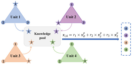
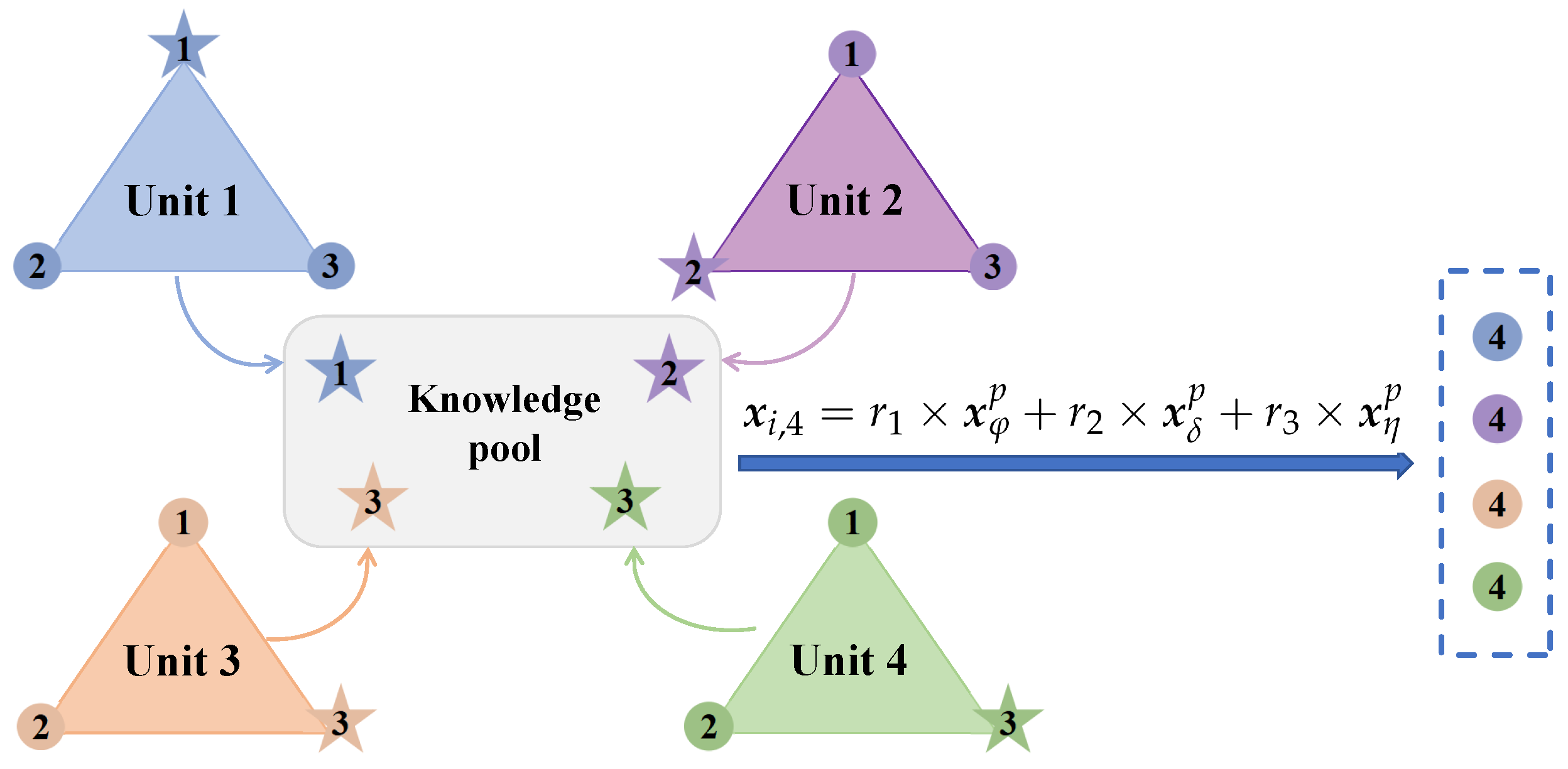
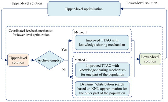
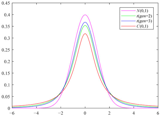
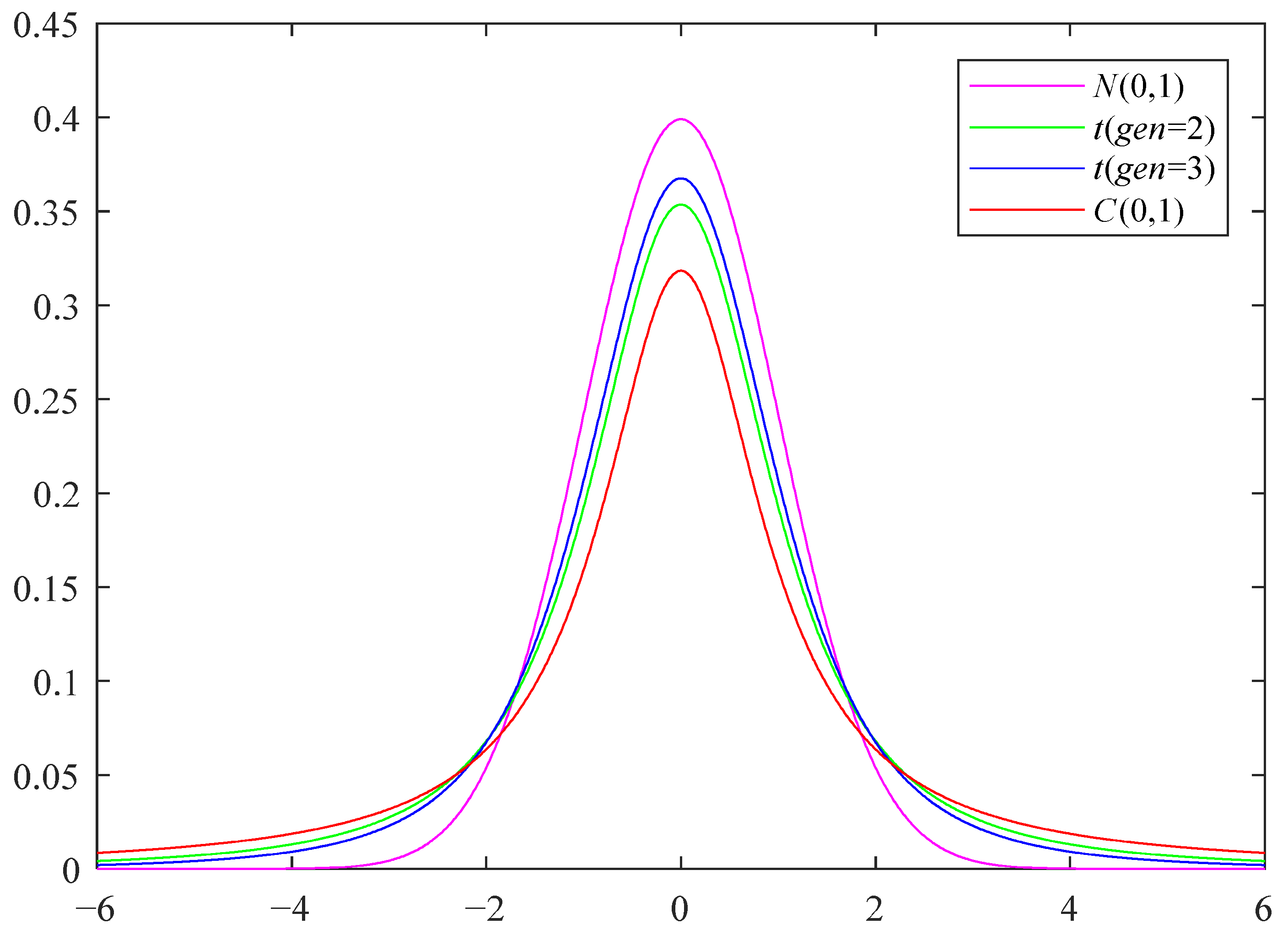
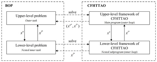
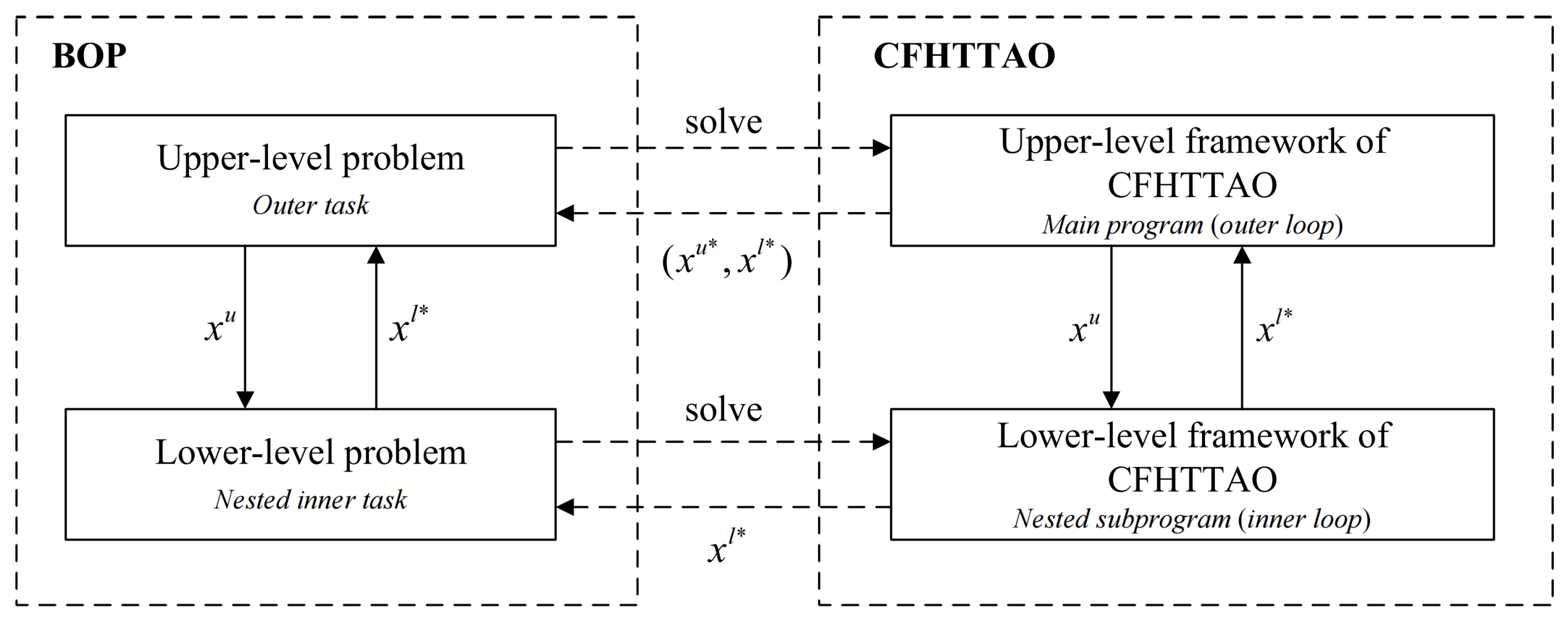
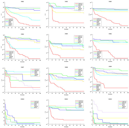
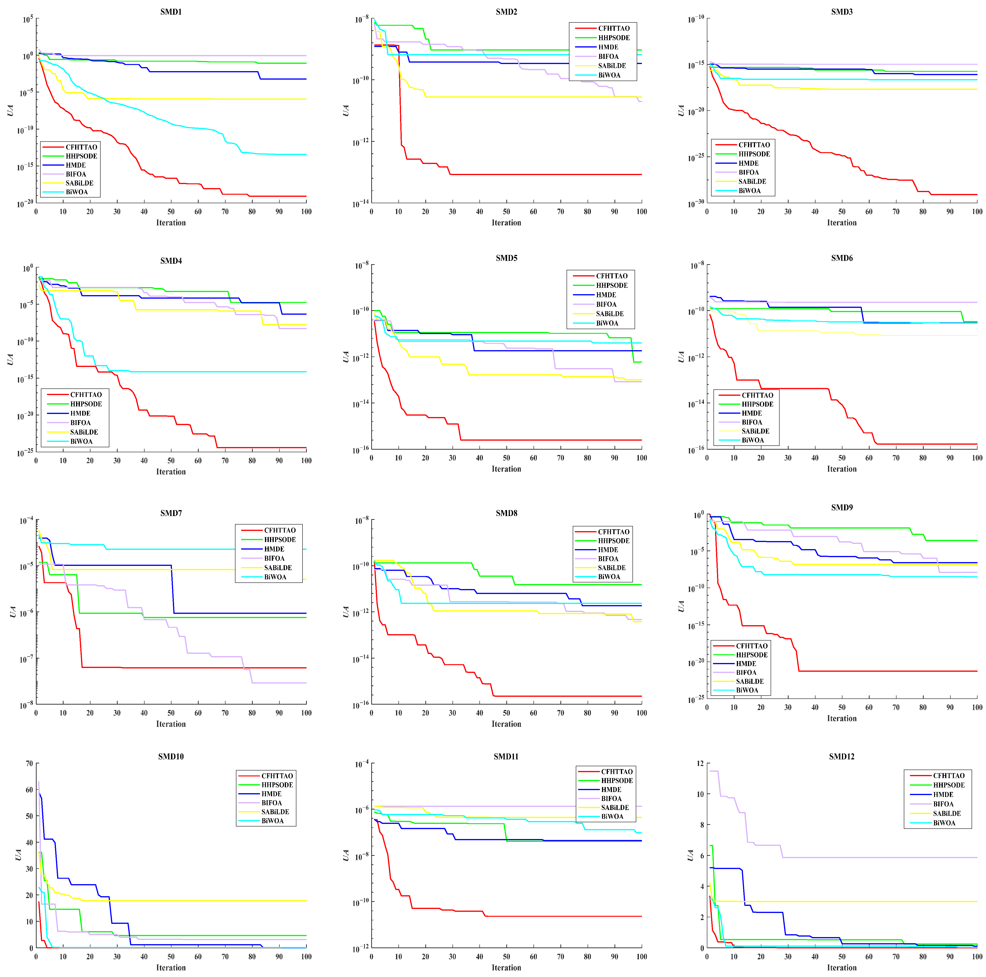
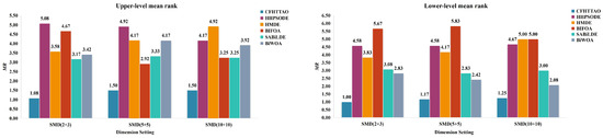
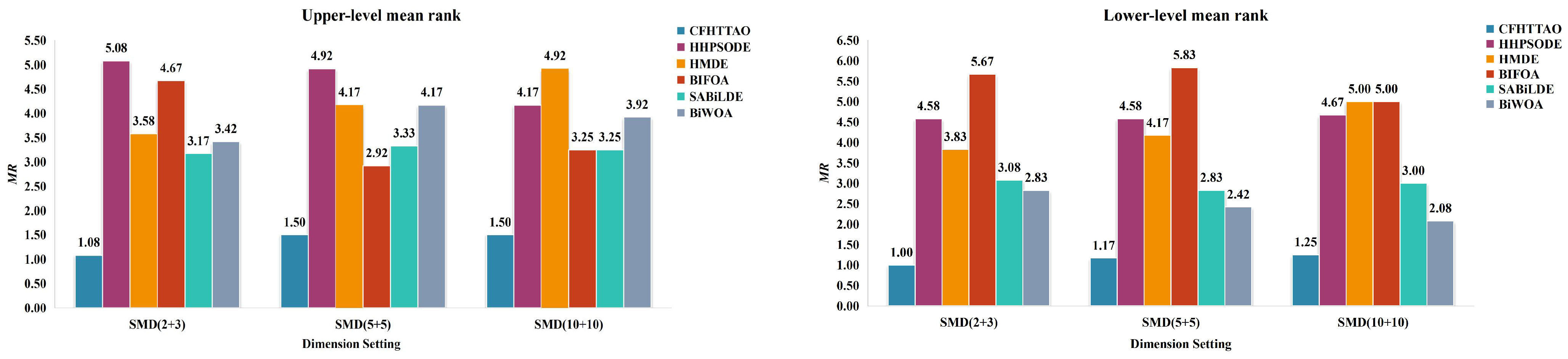

Disclaimer/Publisher’s Note: The statements, opinions and data contained in all publications are solely those of the individual author(s) and contributor(s) and not of MDPI and/or the editor(s). MDPI and/or the editor(s) disclaim responsibility for any injury to people or property resulting from any ideas, methods, instructions or products referred to in the content. |
© 2026 by the authors. Licensee MDPI, Basel, Switzerland. This article is an open access article distributed under the terms and conditions of the Creative Commons Attribution (CC BY) license.