Bayesian Sequential Analysis of Adverse Events with Binary Data

Abstract

We propose a Bayesian sequential procedure to test hypotheses concerning the relative risk between two specific treatments based on the binary data obtained from the two-arm clinical trial. Our development is based on an optimal sequential test cast within the Bayesian framework. This approach enables us to provide, in a straightforward manner based on the Stopping Rule Principle (SRP), an assessment of the various error probabilities via posterior probabilities and conditional error probabilities. An attractive feature of our approach is the relative simplicity of the calculations involved without having to resort to cumbersome iterative methods of ‘spending the alpha’ and the like. The proposed methods are illustrated using a sequential safety study of adverse events following H1N1 influenza vaccination and are compared with existing sequential approaches. The findings demonstrate that the proposed Bayesian framework provides an efficient and flexible approach for the early detection of adverse events under several different prior distributions of the parameters involved.

1. Introduction

The post-market safety surveillance of vaccines and drugs increasingly relies on sequential monitoring of adverse events, in which data accumulate over time as patients are enrolled, treated, and observed for a pre-specified side effect. Regulatory and public health programs such as the Vaccine Safety Datalink and the FDA’s Sentinel Initiative routinely use a two-arm trail comparison, typically contrasting an exposed (treated) group with an unexposed (control) group to detect an elevated rate of an adverse event as early as possible while controlling the chance of a false alarm. A leading example that motivates this paper is the sequential safety surveillance of the H1N1 influenza vaccine analyzed by ref. [1] and later analyzed by refs. [2,3]. In such studies, the main focus is the relative risk (RR) of an adverse event in the exposed group versus the control group. Because enrollment and follow-up occur sequentially, any valid inferential procedure must account for it in the decision to stop (or continue) the study. For such studies, ref. [2] has developed a linear programming framework and proposed an elaborate alpha-spending approach that minimizes the expected time to signal or the expected sample size of the relative risk (RR) under the sequential hypothesis testing procedure. Extension to the bounded-width confidence interval was developed in ref. [3]. However, this approach requires substantial and cumbersome calculations in order to determine the sequence of stopping boundaries, and may not achieve the desired overall Type I error probability.

In this paper, we utilize the Bayesian framework to construct a sequential testing procedure of the hypotheses concerning the RR. As will be seen below, this Bayesian approach provides substantially simpler calculations of the probabilities of the various errors associated with these tests of hypotheses. By the Stopping Rule Principle (SRP) (see ref. [4]), posterior distributions only depend on the data actually observed, but not on the stopping rule itself. This property is shown to be particularly attractive for the sequential monitoring of adverse events in which the stopping rule is incidental to the evidentiary content of the data collected up to that point. Ref. [5] exploited this property to construct a modified Bayesian sequential test that augmented the standard Bayesian sequential test with a ‘no-decision’ region and admitted both a Bayesian and a conditional-frequentist interpretation of the resulting error probabilities. More recently, refs. [6,7] introduced and established the existence of a Uniformly Most Powerful Bayesian Test (UMPBT), which provides an explicit bridge between the Bayesian rejection threshold and a corresponding frequentist rejection region and the significance level. The main contribution of this paper is the construction of a complete Bayesian sequential testing framework for the relative risk in a two-arm adverse event surveillance study with binary data. This approach simplifies the computational workflow and enriches the outcome with directly interpretable measures of evidence instead of using cumbersome alpha-spending calculations.

In Section 2, we consider the testing problem of general hypotheses and related inference problems to the RR, $\gamma$, entirely within the Bayesian framework. Instead of determining a value of $\gamma$ under $H_1$ to calculate the sequential test statistics, the Bayesian sequential test uses the entire alternative support to calculate the corresponding Bayes factor. The resulting sequential Bayesian test does not necessitate any alpha-spending calculations (of the type provided by ref. [2]). Additionally, we present a modified Bayesian test (as was advocated in ref. [5]; see their Section 3 in particular) that benefits from an easily calculated conditional error probabilities and has both a classical (conditional) frequentist as well as Bayesian interpretation. In Section 3, we apply our Bayesian sequential test and the modified Bayesian sequential test to the data discussed in refs. [2,3] under different alternatives, as well as different priors. Specifically, based on the modified Bayesian test, we calculate the conditional Type I or Type II error probability for each data point with the corresponding decision we make. Furthermore, we connect our results to UMPBT and some simulations that can be compared from the frequentist perspective. In Section 4, we compare our results with the results presented in refs. [2,3] and provide some closing remarks.

2. The Bayesian Framework for Binomial Probabilities

2.1. Statistical Framework

Consider a clinical experiment involving a finite population of $N_0$ patients. The patients arrive sequentially and are classified according to two binary attributes: whether they were assigned to receive one of the two available treatments A or B and whether they exhibited a particular side effect (Yes or No) of interest. Having classified in this manner the first n patients, $(1\le n\le N_0)$, the results are summarized in the following $2\times 2$ table, Table 1 below.

Table 1. Table of n items with two treatment groups.

Presenting Side Effect
			$\mathit{No}:\mathit{Y}=\mathbf{0}$	$\mathit{Yes}:\mathit{Y}=\mathbf{1}$
		A	$n_{00}$	$n_{01}$	$n_A$
	Treatment Group
		B	$n_{10}$	$n_{11}$	$n_B:=n-n_A$
	Totals:		$n-S_n^Y$	$S_n^Y$	n

For a give n, the distribution of these four counts is the multinomial distribution, so that

$$\underset{\sim }{n}={(n_{00},n_{10},n_{01},n_{11})}^{\prime }\sim \mathrm{MN}(n,\underset{\sim }{p}),$$

where $\underset{\sim }{p}:={(p_{00},p_{10},p_{01},p_{11})}^{\prime }$ is the vector of the corresponding probabilities, ${\sum }_i{\sum }_j{p}_{ij}=1$ along with ${\sum }_i{\sum }_j{n}_{ij}=n$. Note that the counts in Table 1 follow, marginally for a given n, the Binomial distribution, $n_{ij}\sim \mathrm{B}(n,p_{ij}),i,j=0,1$. In fact, as our sampling of units for classification is conducted sequentially, one at a time, we find it useful to denote by ${\underset{\sim }{z}}^{(k)}={(z_{00,k},z_{10,k},z_{01,k},z_{11,k})}^{\prime }\sim \mathrm{MN}(1,\underset{\sim }{p})$, with ${\sum }_i{\sum }_j{z}_{ij,k}=1$, for each sampling stage $k=1,2,\dots$, in which case,

$$\underset{\sim }{n}={\displaystyle \sum _{k=1}^n}{\underset{\sim }{z}}^{(k)},\mathrm{and}{n}_{ij}={\displaystyle \sum _{k=1}^n}{z}_{ij,k},$$

In the design of the two-arm clinical trial, in which the patients (who are arriving sequentially) are assigned at random to receive one of two available treatments, with some known probability, $p_0$ and $q_0:=1-p_0$, respectively, resulting with $n_A=n_{00}+n_{01}$ of the patients receiving treatment A and $n_B:=n-n_A$ of them receiving treatment B. Accordingly, for a given n,

$$n_A\sim \mathrm{B}(n,p_0),\mathrm{with}{p}_0\equiv p_{00}+p_{01},(p_0\mathrm{fixed}\mathrm{and}\mathrm{known}),$$

Similarly, given n, $n_B\sim \mathrm{B}(n,q_0)$, once assigned to one of the two treatment groups, the patients are subsequently observed during a fixed-length monitoring window for an ‘event’ of interest, such as the post-treatment expression of an adverse side effect, which we generically denote $Y=1$ for ‘present’ and $Y=0$ for a ‘absent’. We denote by ${\vartheta }_A$ and by ${\vartheta }_B$ the conditional probability for expressing (presenting) the monitored side effect given that the patient received Treatment A or Treatment B, respectively. Accordingly, we have

$${\vartheta }_A=\text{Pr}(Y=1\mid \mathrm{Group}\mathrm{A})\mathrm{and}{\vartheta }_B=\text{Pr}(Y=1\mid \mathrm{Group}\mathrm{B}),$$

as well as

$$p_{00}=(1-{\vartheta }_A)\times p_0,\mathrm{and}{p}_{01}={\vartheta }_A\times p_0,$$

so that $p_{00}+p_{01}=p_0$, as desired by design.

For such a study, one is interested in making an inference concerning the unknown probabilities ${\vartheta }_A$ and ${\vartheta }_B$, and, more importantly, concerning the relative risk (RR) of the two treatments to express the monitored side effect, namely, $\gamma ={\vartheta }_A/{\vartheta }_B$. Note that, under this two-arm clinical trial, the (total) probability for presenting the monitored side effect, which we denote by $\eta$, is therefore

$$\text{Pr}(Y=1)={\vartheta }_A{p}_0+{\vartheta }_B{q}_0=\eta .$$

Hence, we immediately obtain that, given an observed side effect, the conditional probability it may be attributed to Treatment A as

$$\theta (\gamma ):=\text{Pr}(\mathrm{Group}\mathrm{A}\mid Y=1)={\displaystyle \frac{{\vartheta }_A{p}_0}{\eta }}={\displaystyle \frac{{\vartheta }_A{p}_0}{{\vartheta }_A{p}_0+{\vartheta }_B{q}_0}}\equiv {\displaystyle \frac{1}{1+z_0/\gamma }},$$

(1)

where we have put $z_0=(1-p_0)/p_0$ to indicate the known matching odds of patients assigned to the treatment B rather than to treatment A. The matching ratio $z_0$ could be thought as the ratio of the number of patients assigned to treatment B relative to the number of patients assigned to treatment A.

Having classified the first n patients according to the above table, we denote by $S_n^Y:=n_{01}+n_{11}$ the total number of patients presenting the monitored side effect (i.e., $Y=1$), and we denote by $X\equiv n_{01}$ the number of patients in Treatment group A that presented the monitored side effect. Clearly, given n, $X\sim \mathrm{B}(n,p_{01}={\vartheta }_A\times p_0)$. However, since it is also given that n, $S_n^Y\sim \mathrm{B}(n,\eta )$, we give n and $\{S_n^Y=m\}$, $X\sim \mathrm{B}(m,\theta (\gamma ))$. Refs. [2,3,8] refer to m as the ‘time’ index for this two-arm binomial experiment. Accordingly, given n, the statistic $S_n^Y$ can be used for inference on the unknown parameter $\eta$, whereas, given n and $\{S_n^Y=m\}$, the count X (out of m) can be used for inference on the unknown parameter $\theta (\gamma )$ and hence of the relative risk parameter $\gamma$.

For the ‘simple’ $\mathrm{B}(n,\eta )$ case, ref. [9] considered the sequential test

$$H_0:\eta \le {\eta }_0\mathrm{against}{H}_1:\eta >{\eta }_0,$$

(2)

for some specified ${\eta }_0$, ${\eta }_0\in (0,1)$, which continues the sampling process as long as the null hypothesis, $H_0$, is not rejected, and stops the sampling process once there is sufficient ‘evidence’ to reject it. More specially, for given desired probabilities of the Type I error $\alpha$ and the Type II error $\beta$ at a given ${\eta }_1>{\eta }_0$, they determined the corresponding sample size $N_0^{*}$ and a critical (boundary) test value $k^{*}$ needed to achieve an ‘optimal’ fixed-sample UMP test of the hypotheses in (2). Since the observations leading to the data in Table 1 become available, sequentially, one at a time or in batches, the collection of the data ceases once the observed total number of patients exhibiting the monitored side effect, $S_n^Y$, exceeds the predefined threshold $k^{*}$, leading to the stopping time

$$M=inf\{n>k^{*}:S_n^Y>k^{*}\},$$

(3)

which has the Negative Binomial distribution, $M\sim \mathrm{NB}(k^{*}+1,\eta )$, on the integers $\{k^{*}+1,k^{*}+2,\dots \}$. Accordingly, the proposed $(\alpha ,\beta )$-optimal sequential test of (2) may be written as

$${\text{Test}}_{\text{seq}}:=\left\{\begin{array}{cc}\mathrm{if}M\le N_0^{*}\hfill & \mathrm{stop}\mathrm{and}\mathrm{reject}{H}_0\mathrm{in}(2)\hfill \\ \mathrm{if}M>N_0^{*}\hfill & \mathrm{do}\mathrm{not}\mathrm{reject}{H}_0\mathrm{in}(2)\hfill \end{array}\right..$$

(4)

Note that, in either case, the final number of observations at ‘termination’ is $M^{*}=min\{M,N_0^{*}\}$, which is the total number of observations collected and used to arrive at a conclusion for the test for (2). Note, however, that, unlike the Sequential Probability Ratio Test (SPRT), the sequential collection of the data under the Stopping Rule (3) is continued as long as $H_0$ is not rejected. Accordingly, upon ’termination’ (either by reaching the maximal number of observations $N_0^{*}$ or by rejecting $H_0$ beforehand), $S_{M^{*}}^Y\in \{0,1,2,\dots ,k^{*}+1\}$.

Refs. [2,10] have considered the above two-arm binomial experiment and the relative risk (RR), $\gamma ={\vartheta }_A/{\vartheta }_B$, of the two treatments to present the monitored side effect. Thus, they considered the testing problem of the hypotheses concerning the parameter $\gamma$ in the form

$$H_0:\gamma =1\mathrm{against}{H}_1:\gamma >1,$$

(5)

which are equivalent to the hypotheses $H_0:{\vartheta }_A={\vartheta }_B$ against $H_1:{\vartheta }_A>{\vartheta }_B$.

For a specified matching allocation ratio between the control group and the treatment group, $z_0$, we denote ${\theta }_0:={(1+z_0)}^{-1}$. We note that the hypotheses in (5) can be stated equivalently in terms of $\theta \equiv \theta (\gamma )\equiv \gamma /(z_0+\gamma )$ as

$$H_0:\theta ={\theta }_0(\mathrm{i}.\mathrm{e}.,\mathrm{with}\gamma =1)\mathrm{against}{H}_1:\theta >{\theta }_0(\mathrm{i}.\mathrm{e}.,\mathrm{with}\gamma >1).$$

(6)

For instance, if the matching allocation ratio is 1:1 (balanced), then $z_0=1$ and therefore ${\theta }_0=1/2$, leading to the test of

$$H_0:\theta =1/2\mathrm{against}{H}_1:\theta >1/2.$$

Hence, the optimal sequential test of ref. [9] for hypotheses in the form of (2) can be applied in this current situation also.

2.2. The Standard Bayesian Test

Suppose that for a given m and unknown $\theta \in (0,1)\equiv \Theta$, a binomial random variable, $X_m\sim \mathrm{B}(m,\theta )$ with a $pmf$ given by

$$p(x\mid \theta ,m)=\text{Pr}(X_m=x\mid \theta ,m)=\left({\displaystyle \genfrac{}{}{0.0pt}{}{m}{x}}\right){\theta }^x{(1-\theta )}^{m-x}\mathbf{I}[x=0,1,\dots ,m].$$

We will see below that the structure of the hypotheses in (2) can generally be formulated as

$$H_0:\theta \in {\Theta }_0\mathrm{against}{H}_1:\theta \in {\Theta }_1$$

(7)

for some ${\Theta }_0\subset \Theta$ and ${\Theta }_1=\Theta -{\Theta }_0$. We assume that, given that the hypothesis $H_i$ is true, $\theta$ has a proper prior $pdf$, $p_i(·)$ over ${\Theta }_i$, $i=0,1$, so that

$${\int }_{{\Theta }_i}{p}_i(\theta )d\theta =1,i=0,1.$$

Accordingly, the test of the hypotheses in (7) can equivalently be formulated as the simple hypotheses concerning the marginal distribution of $X_m$, namely,

$$H_0:X_m\sim f_{0,m}(x)\mathrm{against}{H}_1:X_m\sim f_{1,m}(x),$$

(8)

where, for a given m and $i=0,1$, $f_{i,m}(·)$ is the marginal distribution of $X_m$ under $H_i$, given by

$$f_{i,m}(x):={\int }_{{\Theta }_i}p(x\mid \theta ,m)p_i(\theta )d\theta ,$$

respectively. In the Bayesian framework, one typically assumes that the prior probability that $H_0$ is true is $\text{Pr}(H_0)={\pi }_0$ for some $0<{\pi }_0<1$ and then proceeds to obtain the posterior probability of $H_0$ being true, given the data $\{X_m=x\}$, namely $\text{Pr}(H_0\mid X_m=x)$, where, in the case of the hypotheses (8),

$$\text{Pr}(H_0\mid X_m=x)={\displaystyle \frac{f_{0,m}(x){\pi }_0}{f_{0,m}(x){\pi }_0+f_{1,m}(x)(1-{\pi }_0)}}={\displaystyle \frac{\ell \times B_m(x)}{1+\ell \times B_m(x)}},$$

(9)

where we have substituted $\ell :={\pi }_0/(1-{\pi }_0)$ and $B_m(x):=f_{0,m}(x)/f_{1,m}(x)$. The ratio $B_m(x)$ is the so-called Bayes factor of $H_0$ to $H_1$ (see, for example, ref. [5]). Note that when ${\pi }_0=1/2$, $\ell \equiv 1$, which indicates that the prior probability of the null hypothesis is equal to the prior probability of the alternative hypothesis. The posterior probability of $H_0$ being true, given the data $\{X_m=x\}$, simplifies to

$$\text{Pr}(H_0\mid X_m=x)={\displaystyle \frac{B_m(x)}{1+B_m(x)}}.$$

(10)

Hence, in this basic fixed-sample setup, the Bayesian would simply reject $H_0$ in favor of $H_1$ if $\text{Pr}(H_0\mid X_m=x)<{\pi }_0\equiv 1/2$, or, equivalently, if $B_m(x)<1$. That is, for a given m and $\ell =1$, the Bayesian (fixed-sample) test is

$${\text{Test}}_{\text{Bayes}}:=\left\{\begin{array}{cc}\mathrm{if}{B}_m(x)<1\hfill & \mathrm{Reject}{H}_0\mathrm{in}(8)\hfill \\ \mathrm{if}{B}_m(x)\ge 1\hfill & \mathrm{Accept}{H}_0\mathrm{in}(8).\hfill \end{array}\right.$$

(11)

However, the Bayesian test in (11) might lead to certain ambiguities, especially whenever the value of the Bayes factor $B_m(x)$ is close to the boundary of 1. Based on ref. [11], ref. [12] suggests varying levels of ‘rejection of $H_0$’, all according to the amount of evidence in the data measured by the index $J_B={log}_{10}(B_m(x))$, as presented in Table 2.

Table 2. The values of Bayes factor $B_m$ as a summary of the evidence provided by the data.

${\mathit{J}}_{\mathit{B}}$	${\mathit{B}}_{\mathit{m}}$	Evidence Against ${\mathit{H}}_0$
$-1/2$ to 0	$0.3162$ to 1	Not worth more than a bare mention
$-1$ to $-1/2$	$0.1$ to $0.3162$	Substantial
$-2$ to $-1$	$0.01$ to $0.1$	Strong
<$-2$	<0.01	Decisive

Accordingly, one would substantially reject $H_0$ if $-1<J_B<-1/2$ and would strongly reject $H_0$ if $-2<J_B<-1$ and decisively reject $H_0$ if $J_B<-2$.

As is apparent from (9), the calculations of the Bayes factor require specification of the prior distribution for $\theta$. For the binomial model in (7), a natural choice of prior distributions for $\theta$ would be the conjugate class of distributions over $\Theta =(0,1)$ so that $\theta \sim \mathrm{Beta}(a,b)$ for some parameters $a>0$, $b>0$. Hence, the prior $pdf$ of $\theta$ is given by

$$p(\theta )={\displaystyle \frac{{\theta }^{a-1}{(1-\theta )}^{b-1}}{\mathrm{beta}(a,b)}}\mathbf{I}[0<\theta <1],$$

where $\mathrm{beta}(a,b):={\mathcal{I}}_1(a,b)$ and where, for any $\xi \in [0,1]$,

$${\mathcal{I}}_{\xi }(a,b)={\int }_0^{\xi }{u}^{a-1}{(1-u)}^{b-1}du,$$

is the incomplete beta function. Note that $\mathrm{beta}(a,b)-{\mathcal{I}}_{\xi }(a,b)={\mathcal{I}}_{1-\xi }(b,a)$. With this (conjugate) Beta prior distribution for $\theta$ over $\Theta =(0,1)$, the posterior distribution of $\theta$, given the data $X_m=x$, is the $\mathrm{Beta}(x+a,m-x+b)$ distribution, so that, given m and $X_m=x$,

$$p(\theta \mid X_m)={\displaystyle \frac{{\theta }^{x+a-1}{(1-\theta )}^{m-x+b-1}}{\mathrm{beta}(x+a,m-x+b)}}\mathbf{I}[0<\theta <1].$$

(12)

Furthermore, in this case, the marginal probability distribution of $X_m$ is the Beta-Binomial distribution, given by

$$f_m(x)=\text{Pr}(X_m=x)=\left({\displaystyle \genfrac{}{}{0.0pt}{}{m}{x}}\right){\displaystyle \frac{\mathrm{beta}(a+x,m-x+b)}{\mathrm{beta}(a,b)}}\mathbf{I}[x=0,1,\dots ,m].$$

As an immediate application, consider the binomial experiment, as summarized in Table 1 above, in which the sequential collection of the data was terminated after n observations according to the stopping rule in (3), so that, for the given n and $\{S_n^Y=m\}$, $X_m\sim \mathrm{B}(m,\theta (\gamma ))$, where, as in (6), $\theta \equiv \theta (\gamma )=\gamma /(z_0+\gamma )$ with the known value $z_0$. We remind the reader that, according to the Stopping Rule Principle (SRP), posterior probabilities, as evidentiary data measures, remain unaffected by the optional Stopping Rule for the data collection; see ref. [4] (p. 74) or ref. [13] (p. 502). Hence, in this case also, with the stopping time M in (3), the expression (9) for the posterior probability of $H_0$ holds true, also given the event ${\mathcal{A}}_{nm}:=\left\{(M=n)\mathrm{and}(S_n^Y=m)\right\}$ for some $n\ge m$ and $m\in \{0,1,2,\dots \}$. That is

$$\text{Pr}(H_0\mid X_m=x,{\mathcal{A}}_{nm})\equiv \text{Pr}(H_0\mid X_m=x)={\displaystyle \frac{\ell \times B_m(x)}{1+\ell \times B_m(x)}}.$$

In similarity to the hypotheses in (6), we consider two additional cases of hypotheses concerning the RR parameter $\gamma$. In all cases, we will assume equal prior probabilities of the null and the alternative hypotheses so that, in all cases, we take ${\pi }_0=1/2$ (so that $\ell =1$) in (9).

• Case 1: We are interested in testing of $H_0:\gamma =1$ against $H_1:\gamma \ne 1$, which, with ${\theta }_0={(1+z_0)}^{-1}$, can readily be seen as equivalent to the testing of

  $$H_0^{(1)}:\theta ={\theta }_0\mathrm{against}{H}_1^{(1)}:\theta \ne {\theta }_0.$$

  (13)

  In this case, for $x=0,1,\dots ,m$, the marginal distributions of $X_m$ under $H_0^{(1)}$ and $H_1^{(1)}$ are

  $$f_{0,m}^{(1)}(x)=\left({\displaystyle \genfrac{}{}{0.0pt}{}{m}{x}}\right){\theta }_0^x{(1-{\theta }_0)}^{m-x}$$

  and

  $$f_{1,m}^{(1)}(x)=\left({\displaystyle \genfrac{}{}{0.0pt}{}{m}{x}}\right){\displaystyle \frac{\mathrm{beta}(a+x,m-x+b)}{\mathrm{beta}(a,b)}},$$

  respectively. Hence, the Bayes factor of $H_0^{(1)}$ to $H_1^{(1)}$ in (13) is

  $$B_m^{(1)}(x)={\displaystyle \frac{f_{0,m}^{(1)}(x)}{f_{1,m}^{(1)}(x)}}={\displaystyle \frac{\mathrm{beta}(a,b)\times {\theta }_0^x{(1-{\theta }_0)}^{m-x}}{\mathrm{beta}(a+x,m-x+b)}}.$$

  (14)

  Accordingly, upon termination of the observation process at $\{M=n\}$ for some n, with a given total number of observed side effects $\{S_n^Y=m\}$, of which $X_m=x$ of them are ‘attributed’ to Treatment A, we may calculate the value of the Bayes factor $B_m^{(1)}(x)$, in (14), for any choice of $a,b$ and $z_0$. Therefore, we can obtain the corresponding posterior probability of $H_0^{(1)}$ being true (given the data $\{X_m=x\}$), as given in (19) below.

• Case 2: In a similar fashion, the testing of $H_0:\gamma =1$ against $H_1:\gamma >1$, which, with ${\theta }_0={(1+z_0)}^{-1}$, can readily be seen as equivalent to the testing of

  $$H_0^{(2)}:\theta ={\theta }_0\mathrm{against}{H}_1^{(2)}:\theta >{\theta }_0,$$

  (15)

  In this case also, with equal prior probabilities for $H_0^{(2)}$ and $H_1^{(2)}$ (i.e., ${\pi }_0=1/2$), we have for $x=0,1,\dots ,m$,

  $$f_{0,m}^{(2)}(x)=\left({\displaystyle \genfrac{}{}{0.0pt}{}{m}{x}}\right){\theta }_0^x{(1-{\theta }_0)}^{m-x}$$

  and

  $$f_{1,m}^{(2)}(x)=\left({\displaystyle \genfrac{}{}{0.0pt}{}{m}{x}}\right){\displaystyle \frac{{\mathcal{I}}_{1-{\theta }_0}(m-x+b,a+x)}{{\mathcal{I}}_{1-{\theta }_0}(b,a)}}.$$

  Hence, the Bayes factor of $H_0^{(2)}$ to $H_1^{(2)}$ in (15) is

  $$B_m^{(2)}(x)={\displaystyle \frac{f_{0,m}^{(2)}(x)}{f_{1,m}^{(2)}(x)}}={\displaystyle \frac{{\mathcal{I}}_{1-{\theta }_0}(b,a)\times {\theta }_0^x{(1-{\theta }_0)}^{m-x}}{{\mathcal{I}}_{1-{\theta }_0}(m-x+b,a+x)}}.$$

  (16)

  Here also, upon termination of the observation process at $\{M=n\}$ for some n, with a given total number of observed side effects $\{S_n^Y=m\}$, of which $X_m=x$ of them are ‘attributed’ to Treatment A, we may calculate the value of the Bayes factor $B_m^{(2)}(x)$, in (16), for any choice of a, b and $z_0$ and therefore obtain the corresponding posterior probability of $H_0^{(2)}$ being true (given the data $\{X_m=x\}$), as given in (19) below.

• Case 3: Here, we test $H_0:\gamma \le 1$ against $H_1:\gamma >1$, which is equivalent to testing

  $$H_0^{(3)}:\theta \le {\theta }_0\mathrm{against}{H}_1^{(3)}:\theta >{\theta }_0,$$

  (17)

  with ${\theta }_0={(1+z_0)}^{-1}$. In this case also, with equal prior probabilities for $H_0^{(3)}$ and $H_1^{(3)}$, (i.e., ${\pi }_0=1/2$), we have, for $x=0,1,\dots ,m$,

  $$f_{0,m}^{(3)}(x)=\left({\displaystyle \genfrac{}{}{0.0pt}{}{m}{x}}\right){\displaystyle \frac{{\mathcal{I}}_{{\theta }_0}(a+x,m-x+b)}{{\mathcal{I}}_{{\theta }_0}(a,b)}}$$

  and

  $$f_{1,m}^{(3)}(x)=\left({\displaystyle \genfrac{}{}{0.0pt}{}{m}{x}}\right){\displaystyle \frac{{\mathcal{I}}_{1-{\theta }_0}(m-x+b,a+x)}{{\mathcal{I}}_{1-{\theta }_0}(b,a)}}.$$

  Hence, the Bayes factor of $H_0^{(3)}$ to $H_1^{(3)}$ in (17) is

  $$B_m^{(3)}(x)={\displaystyle \frac{f_{0,m}^{(3)}(x)}{f_{1,m}^{(3)}(x)}}={\displaystyle \frac{{\mathcal{I}}_{1-{\theta }_0}(b,a)\times {\mathcal{I}}_{{\theta }_0}(a+x,m-x+b)}{{\mathcal{I}}_{{\theta }_0}(a,b)\times {\mathcal{I}}_{1-{\theta }_0}(m-x+b,a+x)}}.$$

  (18)

  Clearly, the calculation of the posterior probability is straightforward, as in the previous cases. In fact, in all Cases 1–3, we reject $H_0^{(i)}$ if $B_m^{(i)}<1$ and report the respective posterior probabilities of $H_0^{(i)}$ and $H_1^{(i)}$ being true as

  $$\tilde{\alpha }\left(B_m^{(i)}(x)\right)=\text{Pr}\left(H_0^{(i)}\mid X_m=x\right)={\displaystyle \frac{B_m^{(i)}(x)}{1+B_m^{(i)}(x)}},\mathrm{for}i=1,2,3;$$

  (19)

  $$\tilde{\beta }\left(B_m^{(i)}(x)\right)=\text{Pr}\left(H_1^{(i)}\mid X_m=x\right)={\displaystyle \frac{1}{1+B_m^{(i)}(x)}},\mathrm{for}i=1,2,3.$$

  (20)

  Accordingly, in all of these three cases, the Bayesian test can be presented as

  $${\text{Test}}_{\text{Bayes}}:=\left\{\begin{array}{cc}\mathrm{if}{B}_m^{(i)}(x)<1,\hfill & \mathrm{Reject}{H}_0^{(i)}\mathrm{and}\mathrm{report}\mathrm{the}\hfill \\ \hfill & \mathrm{posterior}\mathrm{probability}\tilde{\alpha }\left(B_m^{(i)}(x)\right)\hfill \\ \mathrm{if}{B}_m^{(i)}(x)\ge 1,\hfill & \mathrm{Accept}{H}_0^{(i)}\mathrm{and}\mathrm{report}\mathrm{the}\hfill \\ \hfill & \mathrm{posterior}\mathrm{probability}\tilde{\beta }\left(B_m^{(i)}(x)\right),\hfill \end{array}\right.$$

  (21)

  for $i=1,2,3$. Clearly, the Bayesian tests in (21) can incorporate Jeffrey’s criteria, as in Table 2, to determine the strength of the data in evidence to support the rejection of the respective $H_0^{(i)}$.

Note that, to fully apply the test of the hypotheses in (8), one would need to specify the values of the prior distribution parameters a and b and matching allocation ratio between the two treatment groups, $z_0$, in the calculations of $B_m^{(i)}(x)$, $i=1,2,3$.

2.3. The Modified Bayesian Test

In the spirit of Table 2, we modify the standard Bayesian test to include a ‘no-decision region’. This would often be a useful approach in a situation when there is an ambiguous result that appears.

As advocated and suggested in ref. [5], we modify the Bayesian test in (8) to include a no-decision region. The modified Bayesian test takes the form

$${\text{Test}}_{\text{M-Bayes}}:=\left\{\begin{array}{cc}\mathrm{if}{B}_m(x)<r\hfill & \mathrm{Reject}{H}_0\mathrm{and}\mathrm{report}\mathrm{the}\mathrm{conditional}\hfill \\ \hfill & \mathrm{error}\mathrm{probability}{\alpha }^{*}\left(B_m(x)\right)\hfill \\ \mathrm{if}r\le B_m(x)\le u\hfill & \mathrm{make}\mathrm{no}\mathrm{decision}\hfill \\ \mathrm{if}{B}_m(x)>u\hfill & \mathrm{Accept}{H}_0\mathrm{and}\mathrm{report}\mathrm{the}\mathrm{conditional}\hfill \\ \hfill & \mathrm{error}\mathrm{probability}{\beta }^{*}\left(B_m(x)\right),\hfill \end{array}\right.$$

(22)

where $r<u$ are two constants, defined and calculated as described in (23) below. For more details about the ‘no-decision region’ and a further explanation and justification in the sequential setting, see the details in Section 3 of ref. [5].

Let $F_0$ and $F_1$ be the cdf of $B_m(x)$ under $H_0$ and $H_1$, respectively. Their inverse $F_0^{-1}$ and $F_1^{-1}$ exist in the range $\mathcal{B}$ of $B_m(x)$. For any $b\in \mathcal{B}$, we let

$$\psi (b):=F_0^{-1}\left(1-F_1(b)\right)\mathrm{and}{\psi }^{-1}(b):=F_1^{-1}\left(1-F_0(b)\right).$$

Accordingly, the decision constants r and u are calculated as

$$\begin{array}{cc}\hfill & r=1\mathrm{and}u=\psi (1)\mathrm{if}\psi (1)\ge 1,\hfill \\ \hfill & r={\psi }^{-1}(1)\mathrm{and}u=1\mathrm{if}\psi (1)<1.\hfill \end{array}$$

(23)

As stated in ref. [5], the posterior probabilities of $H_0$ and $H_1$ could also be interpreted as the conditional error frequentist Type I and Type II probabilities. ${\text{Test}}_{\text{M-Bayes}}$ is also a conditional frequentist test arising from the use of the conditioning statistic

$$S(X)=min\{B_m(X),{\psi }^{-1}(B_m(X))\},$$

(24)

over the domain ${\mathcal{X}}^{*}=\cup {\mathcal{X}}_s\equiv \{0<S(X)<r\}$ (the complement of ${\mathcal{X}}^{*}$ is the no-decision region). Therefore, the conditional error probabilities upon accepting or rejecting $H_0$, given $\{S(X)=s\}$, denoted as ${\alpha }^{*}(s)$ and ${\beta }^{*}(s)$, are given by

$${\alpha }^{*}(s)={\displaystyle \frac{s}{1+s}}\equiv P(H_0|{\mathcal{X}}_s)\mathrm{and}{\beta }^{*}(s)={\displaystyle \frac{1}{1+\psi (s)}}\equiv P(H_1|{\mathcal{X}}_s),$$

(25)

which are in complete agreement with the Bayesian posterior probabilities of $H_0$, given the data provided in (10) (see also (19) and (20)).

3. Example

Ref. [2] reported the results of a sequential study on the side effects of the H1N1 influenza vaccine during the 2009–2010 influenza season (see ref. [1]), which was conducted with an equal allocation between the exposed group, A, and the not-exposed group, B, so that the study design matching constant was $z_0=1$ and, hence, ${\theta }_0=1/2$. The 24 successive data points on $(m,X_m)$ from the study cited are presented in the table below, along with the values of $\widehat{\gamma }\equiv X_m/(m-X_m)$. Applying their iterative ‘sequential’ procedure to the hypotheses of Case 2, ref. [2] determined, for $\alpha =0.05$, that the testing procedure should have been terminated at the 19th-group data point, with $m=222$ and $X_{222}=134$, which resulted with an estimated RR of $\widehat{\gamma }=1.5227$. For Case 3 and a related confidence interval, ref. [3] determined, for $\alpha =0.1$, that the testing procedure should have been terminated at the 18th-group data point, with $m=218$ and $X_{218}=130$, which resulted with an estimated RR of $\widehat{\gamma }=1.4773$.

For comparison, we apply the above Bayesian Beta-Binomial models we propose to these 24 data points under several prior distributions; however, all had a prior mean of $0.5$. Bayes factors are known to depend on the prior specification under the alternative hypothesis, and the sensitivity of Bayes factors to prior assumptions has been widely discussed in the Bayesian literature. For this reason, we consider both non-informative and informative prior specifications in our analysis. The purpose of these examples is not to advocate a universally objective prior, but rather to illustrate the behavior of the proposed sequential testing procedure under commonly used prior structures.

3.1. The Standard Bayesian Test

(I)

Case of non-informative (uniform) prior distribution

We assume a uniform prior distribution for $\theta$, so that $\theta \sim \mathrm{Beta}(a=1,b=1)$. We calculated the Bayes factor $B_m^{(i)}$ and the corresponding posterior probability $\text{Pr}(H_0^{(i)}\mid X_m=x)$, $i=1,2,3$ for the hypotheses tests on the RR, $\gamma$ in the three cases we considered above. We always assume that the prior probability that $H_0$ is true, that is, $\text{Pr}(H_0)={\pi }_0=1/2$. The numerical results are provided in Table 3 below.

Table 3. The values of Bayes factor and posterior probability of $H_0$ for each data point among the three different cases with the uniform prior.

Test	m	${\mathit{X}}_{\mathit{m}}$	$\widehat{\mathit{\gamma }}$	${\mathit{B}}_{\mathit{m}}^{(1)}$	$\text{Pr}({\mathit{H}}_0^{(1)}\mid {\mathit{X}}_{\mathit{m}})$	${\mathit{B}}_{\mathit{m}}^{(2)}$	$\text{Pr}({\mathit{H}}_0^{(2)}\mid {\mathit{X}}_{\mathit{m}})$	${\mathit{B}}_{\mathit{m}}^{(3)}$	$\text{Pr}({\mathit{H}}_0^{(3)}\mid {\mathit{X}}_{\mathit{m}})$
1	12	1	0.0909	0.0381	0.0367	11.1429	0.9176	584.1429	0.9983
2	18	5	0.3846	0.6210	0.3831	9.7691	0.9071	30.4623	0.9682
3	24	11	0.8462	3.7195	0.7881	5.3903	0.8435	1.8984	0.6550
4	30	15	1.0000	4.4784	0.8175	4.4784	0.8175	1.0000	0.5000
5	34	15	0.7895	3.7811	0.7908	7.5689	0.8833	3.0035	0.7502
6	40	17	0.7391	3.3088	0.7679	9.4837	0.9046	4.7325	0.8256
7	46	20	0.7692	3.7458	0.7893	9.8136	0.9075	4.2398	0.8092
8	67	34	1.0303	6.5554	0.8676	5.9790	0.8567	0.8241	0.4518
9	78	39	1.0000	7.1142	0.8768	7.1142	0.8768	1.0000	0.5000
10	100	44	0.7857	3.9342	0.7973	16.9359	0.9442	7.6095	0.8838
11	115	51	0.7969	4.1504	0.8058	18.2614	0.9481	7.7999	0.8864
12	135	63	0.8750	6.9197	0.8737	15.7129	0.9402	3.5415	0.7798
13	167	88	1.1139	8.1376	0.8906	5.3805	0.8433	0.3224	0.2438
14	172	91	1.1235	7.8705	0.8873	5.0685	0.8352	0.2880	0.2236
15	190	107	1.2892	2.4347	0.7089	1.2695	0.5594	0.0429	0.0411
16	197	113	1.3452	1.3341	0.5716	0.6803	0.4049	0.0199	0.0195
17	211	124	1.4253	0.4531	0.3118	0.2278	0.1855	0.0055	0.0054
18	218	130	1.4773	0.2055	0.1704	0.1030	0.0933	0.0022	0.0022
19	222	134	1.5227	0.1003	0.0911	0.0502	0.0478	0.0010	0.0010
20	231	141	1.5667	0.0427	0.0410	0.0214	0.0209	0.0004	0.0004
21	240	148	1.6087	0.0175	0.0172	0.0087	0.0087	0.0001	0.0001
22	245	153	1.6630	0.0060	0.0060	0.0030	0.0030	0.0000	0.0000
23	247	155	1.6848	0.0039	0.0038	0.0019	0.0019	0.0000	0.0000
24	251	157	1.6702	0.0044	0.0044	0.0022	0.0022	0.0000	0.0000

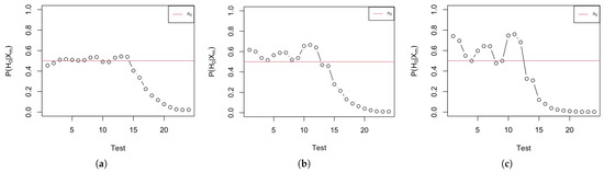
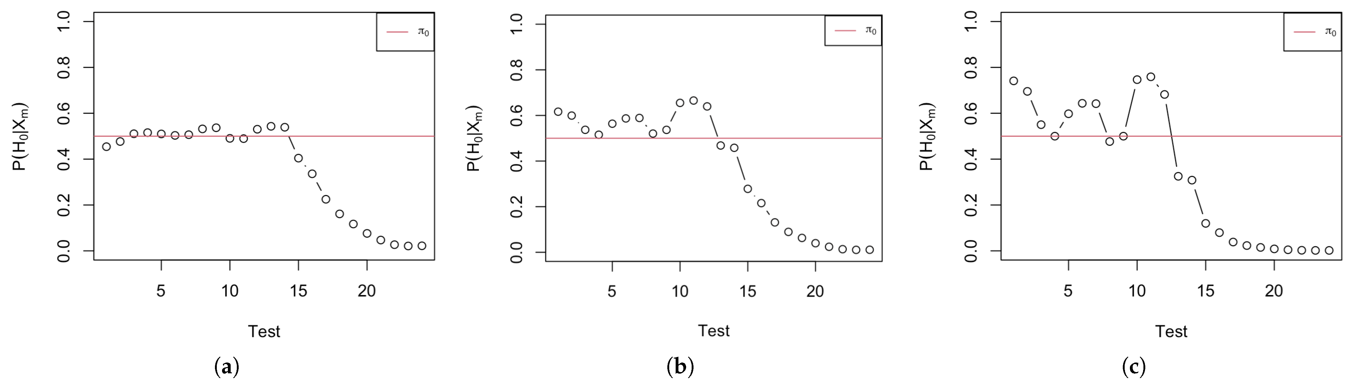
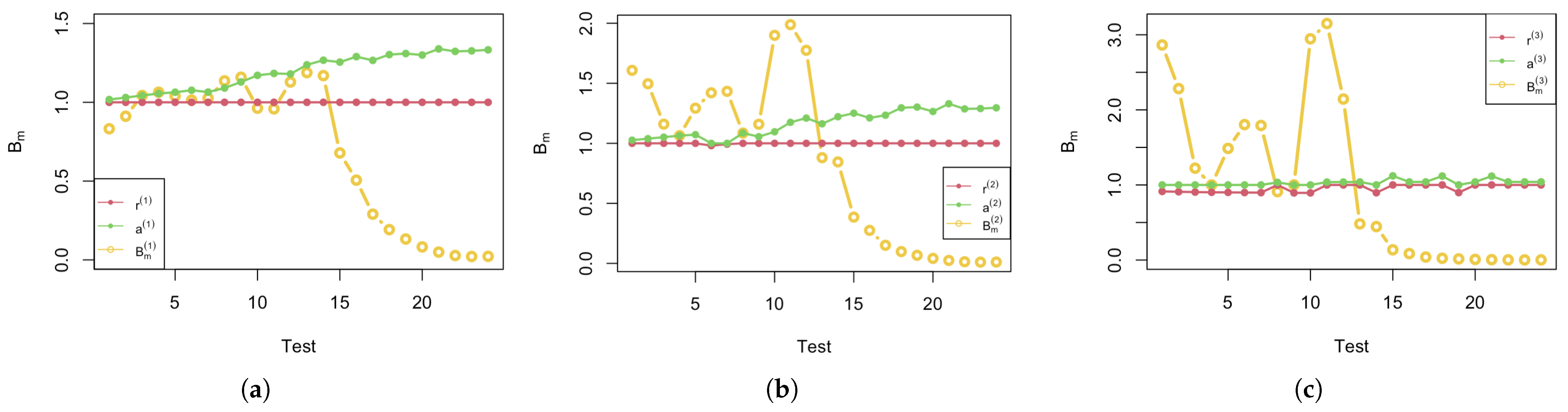
As can be seen, for the hypotheses of Case 1, our Bayesian model above has led to the potentially earlier ‘termination’ at the 18th-group data point with a total of $m=218$ ‘events’, the observed side effect of which $X_m=130$ was noted in the treatment group with an estimated relative risk of $\widehat{\gamma }=X_m/(m-X_m)=1.4773$. For the hypotheses of Case 2, our Bayesian model led to the potentially earlier ‘termination’ at the 17th-group data point with a total of $m=211$ ‘events’, the observed side effect of which $X_m=124$ were noted in the treatment group with an estimated relative risk of $\widehat{\gamma }=1.4253$. The resulting Bayes factors are $B_{218}^{(1)}=0.2055$ and $B_{211}^{(2)}=0.2278$, which are less than $0.3162$ based on the standard shown in Table 2. This leads to a rejection of $H_0^{(i)}$, $i=1,2$ and the posterior probabilities of the null hypothesis, and the alternative hypotheses, given the data, are

$$\text{Pr}(H_0^{(1)}:\gamma =1\mid X_{218}=130)=0.1704,\text{Pr}(H_1^{(1)}:\gamma \ne 1\mid X_{218}=130)=0.8296,$$

and

$$\text{Pr}(H_0^{(2)}:\gamma =1\mid X_{211}=124)=0.1855,\text{Pr}(H_1^{(2)}:\gamma >1\mid X_{211}=124)=0.8145,$$

which are clearly smaller than the assumed prior probability ${\pi }_0=0.5$ of $H_0^{(i)}$, $i=1,2$ being true (marked in a red line in Figure 1).

Figure 1. The posterior probability of $H_0$ for the 24 data points of Table 3: (a) Case 1; (b) Case 2; (c) Case 3.

On the other hand, for the hypotheses of Case 3, one would ‘terminate’ the observation process much earlier, already at the 14th-group data point with a total of $m=172$ ‘events’, the observed side effects of which $X_m=91$ were noted in the treatment group, leading to the estimated relative risk of $\widehat{\gamma }=1.1235$. The resulting Bayes factor is $B_{172}^{(3)}=0.2880$, which is less than $0.3162$ based on the standard shown in Table 2, and the posterior probabilities of the null hypothesis and the alternative hypotheses given the data are

$$\text{Pr}(H_0^{(3)}:\gamma \le 1\mid X_{172}=91)=0.2236,\text{Pr}(H_1^{(3)}:\gamma >1\mid X_{172}=91)=0.7764,$$

which are clearly smaller than the assumed prior probability ${\pi }_0=0.5$ of $H_0^{(3)}$ being true (marked in a red line in Figure 1).

Remark 1.

We point out that, in Case 3, we choose the early ‘termination’ at the 14th-group data point instead of 8th-group data point. At the 8th-group data point with a total of $m=67$ ‘events’, the observed side effects of which $X_m=34$ were noted in the treatment group, leading to the estimated relative risk of $\widehat{\gamma }=X_m/(m-X_m)=1.0303$. The resulting Bayes factor is $B_{67}^{(3)}=0.8241<1$, and the posterior probabilities of the null hypothesis and the alternative hypothesis given the data are

$$\text{Pr}(H_0^{(3)}:\gamma \le 1\mid X_{67}=34)=0.4518,\text{Pr}(H_1^{(3)}:\gamma >1\mid X_{67}=34)=0.5482.$$

Although the value of $\text{Pr}(H_0^{(3)}\mid X_{67}=34)$ is less than $0.5$, following the standard shown in Table 2, the evidence against $H_0^{(3)}$ at the 8th-group data point is not worth more than a bare mention. Therefore, we would substantially reject $H_0^{(3)}$ and stop at the 14th-group data point.

Remark 2.

In Case 3, we observe that the values of Bayes factor at the 4th and 9th-group data point are exactly equal to 1. Due to the data structure, we have the matching allocation ratio $z_0=1$, and, at the 4th-group and 9th-group data points, $m-X_m=X_m$. Moreover, since the mean of the chosen prior distributions is $0.5$, it is not surprising that, at these two specific data points, the values of the Bayes factor are 1.

We further applied Jeffrey’s prior, discussed in ref. [14], as an ‘objective’ and non-informative prior to above three cases since a uniform prior on the parameter $\theta$ does not generally remain uniform under nonlinear transformations of the parameter $\gamma$. Specifically, for the binomial model, Jeffrey’s prior is $\mathrm{Beta}(1/2,1/2)$. Since the results under Jeffrey’s prior are similar to the results we obtained under the uniform prior, we would not give a detailed interpretation of the results under Jeffrey’s prior (shown in Appendix A).

(II)

Case of informative prior distribution

Here, we assume an informative prior distribution for $\theta$ that is induced by determining the values of $(a,b)$ by the following set of two equations:

$$E(\theta )={\displaystyle \frac{1}{1+z_0}}\mathrm{and}\text{Pr}(|\gamma (\theta )-1|\le ϵ\mid \theta )=\delta$$

for some given $\delta$ and $ϵ$ and where $\gamma (\theta )\equiv z_0\times \theta /(1-\theta )$ by (1). In the current example, we have $z_0=1$ and assume $ϵ=0.1$ and $\delta =0.55$. Hence, we ‘solve’ for our prior parameters to obtain $a=b=113.8288$. Note that the informative prior information may be obtained from expert suggestion or by borrowing from previous similar studies. The informative prior presented in this case is only an illustration. Applying the procedure we proposed above, we calculated the Bayes factor $B_m^{(i)}$ and the corresponding posterior probability $\text{Pr}(H_0^{(i)}\mid X_m=x)$, $i=1,2,3$, for the hypotheses testing on $\gamma$ in the three cases we considered above. The numerical results are provided in Table 4 below.

Table 4. The values of Bayes factor and posterior probability of $H_0$ for each data point among different cases with the informative prior.

Test	m	${\mathit{X}}_{\mathit{m}}$	$\widehat{\mathit{\gamma }}$	${\mathit{B}}_{\mathit{m}}^{(1)}$	$\text{Pr}({\mathit{H}}_0^{(1)}\mid {\mathit{X}}_{\mathit{m}})$	${\mathit{B}}_{\mathit{m}}^{(2)}$	$\text{Pr}({\mathit{H}}_0^{(2)}\mid {\mathit{X}}_{\mathit{m}})$	${\mathit{B}}_{\mathit{m}}^{(3)}$	$\text{Pr}({\mathit{H}}_0^{(3)}\mid {\mathit{X}}_{\mathit{m}})$
1	12	1	0.0909	0.8321	0.4542	1.6078	0.6165	2.8646	0.7412
2	18	5	0.3846	0.9115	0.4768	1.4964	0.5994	2.2834	0.6954
3	24	11	0.8462	1.0431	0.5106	1.1597	0.5370	1.2234	0.5502
4	30	15	1.0000	1.0640	0.5155	1.0640	0.5155	1.0000	0.5000
5	34	15	0.7895	1.0398	0.5098	1.2927	0.5638	1.4864	0.5978
6	40	17	0.7391	1.0137	0.5034	1.4210	0.5869	1.8036	0.6433
7	46	20	0.7692	1.0265	0.5065	1.4329	0.5890	1.7917	0.6418
8	67	34	1.0303	1.1360	0.5318	1.0855	0.5205	0.9111	0.4767
9	78	39	1.0000	1.1590	0.5368	1.1590	0.5368	1.0000	0.5000
10	100	44	0.7857	0.9627	0.4905	1.8995	0.6551	2.9465	0.7466
11	115	51	0.7969	0.9583	0.4894	1.9886	0.6654	3.1501	0.7590
12	135	63	0.8750	1.1289	0.5303	1.7747	0.6396	2.1442	0.6820
13	167	88	1.1139	1.1885	0.5431	0.8805	0.4682	0.4817	0.3251
14	172	91	1.1235	1.1693	0.5390	0.8452	0.4581	0.4456	0.3083
15	190	107	1.2892	0.6786	0.4043	0.3855	0.2782	0.1361	0.1198
16	197	113	1.3452	0.5061	0.3360	0.2749	0.2156	0.0862	0.0794
17	211	124	1.4253	0.2901	0.2249	0.1509	0.1311	0.0400	0.0384
18	218	130	1.4773	0.1920	0.1611	0.0983	0.0895	0.0237	0.0231
19	222	134	1.5227	0.1325	0.1170	0.0672	0.0630	0.0151	0.0149
20	231	141	1.5667	0.0824	0.0761	0.0415	0.0399	0.0086	0.0085
21	240	148	1.6087	0.0494	0.0471	0.0248	0.0242	0.0048	0.0047
22	245	153	1.6630	0.0276	0.0269	0.0138	0.0136	0.0025	0.0025
23	247	155	1.6848	0.0216	0.0212	0.0108	0.0107	0.0019	0.0019
24	251	157	1.6702	0.0225	0.0220	0.0113	0.0111	0.0020	0.0019

As can be seen, for the hypotheses of Case 1, based on the standard shown in Table 2, our Bayesian model above led to the potentially earlier ‘termination’ at the 17th-group data point with a total of $m=211$ ‘events’, the observed side effect of which $X_m=124$ was noted in the treatment group with an estimated relative risk of $\widehat{\gamma }=1.4253$. For the hypotheses of Case 2, our Bayesian model led to the potentially earlier ‘termination’ at the 16th-group data point with a total of $m=197$ ‘events’, the observed side effect of which $X_m=113$ was noted in the treatment group with an estimated relative risk of $\widehat{\gamma }=1.3452$. The resulting Bayes factors are $B_{211}^{(1)}=0.2901<0.3162$ and $B_{197}^{(2)}=0.2749<0.3162$. These lead to a rejection of $H_0^{(i)}$, $i=1,2$, and the posterior probabilities of the null hypothesis and the alternative hypothesis given the data are

$$\text{Pr}(H_0^{(1)}:\gamma =1\mid X_{211}=124)=0.2249,\text{Pr}(H_1^{(1)}:\gamma \ne 1\mid X_{211}=124)=0.7751,$$

and

$$\text{Pr}(H_0^{(2)}:\gamma =1\mid X_{197}=113)=0.2156,\text{Pr}(H_1^{(2)}:\gamma >1\mid X_{197}=113)=0.7844,$$

which are clearly smaller than the assumed prior probability ${\pi }_0=0.5$ of $H_0^{(i)}$, $i=1,2$ being true (marked in a red line in Figure 2).

Figure 2. The posterior probability of $H_0$ for the 24 data points of Table 4: (a) Case 1; (b) Case 2; (c) Case 3.

Furthermore, for the hypotheses of Case 3, based on the standard shown in Table 2, the 15th-group data point with a total of $m=190$ ‘events’, the observed side effect of which $X_m=107$ was noted in the treatment group, lead to an estimated relative risk of $\widehat{\gamma }=1.2892$. The resulting Bayes factor is $B_{190}^{(3)}=0.1361<0.3162$, and the posterior probabilities of the null hypothesis and the alternative hypothesis given the data are

$$\text{Pr}(H_0^{(3)}:\gamma \le 1\mid X_{190}=107)=0.1198,\text{Pr}(H_1^{(3)}:\gamma >1\mid X_{190}=107)=0.8802,$$

which is clearly smaller than the assumed prior probability ${\pi }_0=0.5$ of $H_0^{(3)}$ being true (marked in red line in Figure 2).

In conclusion, with the uniform prior, Case 1 would be rejected and ‘terminated’ at the 18th-group data point, Case 2 would be rejected and ‘terminated’ at the 17th-group data point, and Case 3 would be rejected and ‘terminated’ at the 14th-group data point. However, with the informative prior we chose, Case 1 would be rejected and ‘terminated’ at the 17th-group data point, Case 2 would be rejected and ‘terminated’ at the 16th-group data point, and Case 3 would be rejected and ‘terminated’ at the 15th-group data point.

3.2. The Modified Bayesian Test

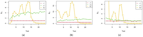
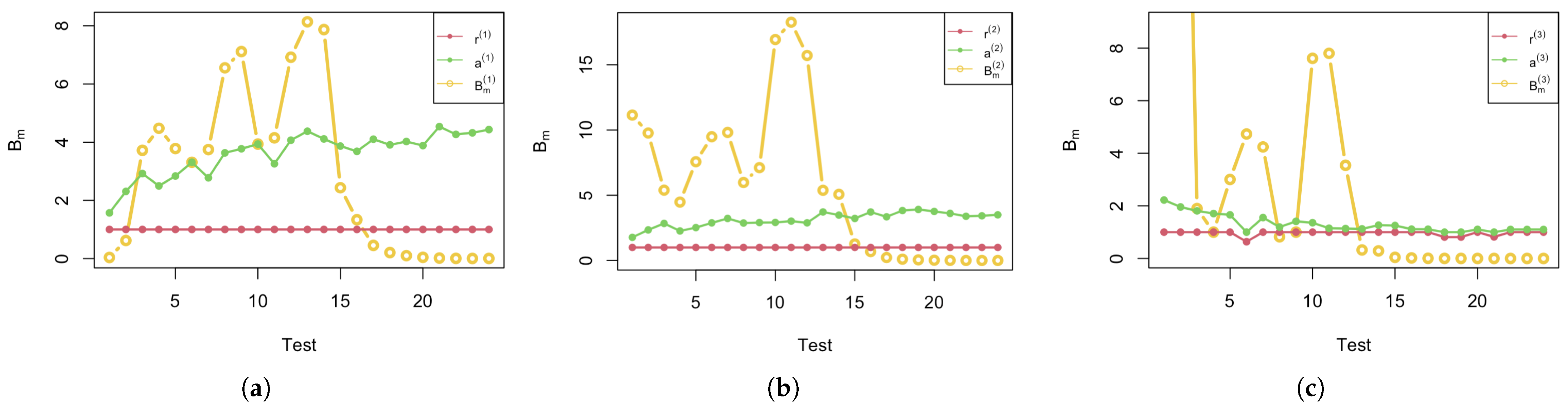
Applying the modified Bayesian test in (22) to Case 1, 2, and 3, along with the same prior structures we discussed above, we analyze the results of the above example again. Under both types of priors, we obtained the same conclusions that were obtained utilizing the standard Bayesian test for the hypotheses $H_0^{(i)}$, $i=1,2,3$ (see Section 3.1). The results corresponding to the non-informative (uniform) prior distributions are shown in Figure 3, Table 5 and Table 6. The results corresponding to the informative prior distributions are shown in Figure 4, Table 7 and Table 8. However, under both prior structures, utilizing the modified Bayesian test, we see that there are several cases with some data points falling into the ‘no-decision’ region. In all cases, we provide the calculated conditional Type I and Type II error probabilities, ${\alpha }^{*}$ and ${\beta }^{*}$, corresponding to the ‘Reject’ or ‘Accept’ decision (see Table 6 and Table 8).

Figure 3. The acceptance and rejection boundaries of $B_m$ for the 24 data points of Table 5: (a) Case 1; (b) Case 2; (c) Case 3.

Table 5. The values of Bayes factor and the boundaries based on it for each data point among different cases with the uniform prior.

Test	m	${\mathit{X}}_{\mathit{m}}$	$\widehat{\mathit{\gamma }}$	${\mathit{B}}_{\mathit{m}}^{(1)}$	${\mathit{r}}^{(1)}$	${\mathit{u}}^{(1)}$	${\mathit{B}}_{\mathit{m}}^{(2)}$	${\mathit{r}}^{(2)}$	${\mathit{u}}^{(2)}$	${\mathit{B}}_{\mathit{m}}^{(3)}$	${\mathit{r}}^{(3)}$	${\mathit{u}}^{(3)}$
1	12	1	0.0909	0.0381	1	1.5710	11.1429	1	1.7715	584.1429	1	2.2226
2	18	5	0.3846	0.6210	1	2.3066	9.7691	1	2.3451	30.4623	1	1.9583
3	24	11	0.8462	3.7195	1	2.9225	5.3903	1	2.8394	1.8984	1	1.8080
4	30	15	1.0000	4.4784	1	2.4971	4.4784	1	2.2645	1.0000	1	1.7083
5	34	15	0.7895	3.7811	1	2.8358	7.5689	1	2.5200	3.0035	1	1.6586
6	40	17	0.7391	3.3088	1	3.3088	9.4837	1	2.8814	4.7325	0.6363	1
7	46	20	0.7692	3.7458	1	2.7747	9.8136	1	3.2207	4.2398	1	1.5532
8	67	34	1.0303	6.5554	1	3.6340	5.9790	1	2.8700	0.8241	1	1.1945
9	78	39	1.0000	7.1142	1	3.7717	7.1142	1	2.9057	1.0000	1	1.4105
10	100	44	0.7857	3.9342	1	3.9342	16.9359	1	2.9138	7.6095	1	1.3574
11	115	51	0.7969	4.1504	1	3.2564	18.2614	1	3.0174	7.7999	1	1.1485
12	135	63	0.8750	6.9197	1	4.0694	15.7129	1	2.8836	3.5415	1	1.1371
13	167	88	1.1139	8.1376	1	4.3758	5.3805	1	3.7172	0.3224	1	1.1233
14	172	91	1.1235	7.8705	1	4.1132	5.0685	1	3.4800	0.2880	1	1.2656
15	190	107	1.2892	2.4347	1	3.8676	1.2695	1	3.2199	0.0429	1	1.2517
16	197	113	1.3452	1.3341	1	3.6836	0.6803	1	3.7146	0.0199	1	1.1136
17	211	124	1.4253	0.4531	1	4.1037	0.2278	1	3.3458	0.0055	1	1.1098
18	218	130	1.4773	0.2055	1	3.9079	0.1030	1	3.8280	0.0022	0.8116	1
19	222	134	1.5227	0.1003	1	4.0227	0.0502	1	3.9134	0.0010	0.8131	1
20	231	141	1.5667	0.0427	1	3.8834	0.0214	1	3.7579	0.0004	1	1.1049
21	240	148	1.6087	0.0175	1	4.5363	0.0087	1	3.6076	0.0001	0.8193	1
22	245	153	1.6630	0.0060	1	4.2679	0.0030	1	3.3872	0.0000	1	1.1018
23	247	155	1.6848	0.0039	1	4.3227	0.0019	1	3.4248	0.0000	1	1.1014
24	251	157	1.6702	0.0044	1	4.4320	0.0022	1	3.4998	0.0000	1	1.1006

Table 6. The decision and corresponding conditional ${\alpha }^{*}$ and ${\beta }^{*}$ for each data point among different cases with the uniform prior (Decision: ‘R’ indicates Reject, ‘A’ indicates Accept, ‘ND’ indicates No Decision, ‘NA’ indicates No Answer).

Test	$\widehat{\mathit{\gamma }}$	${\mathit{B}}_{\mathit{m}}^{(1)}$	Decision	${\mathit{\alpha }}^{*}(\mathbf{or}{\mathit{\beta }}^{*})$	${\mathit{B}}_{\mathit{m}}^{(2)}$	Decision	${\mathit{\alpha }}^{*}(\mathbf{or}{\mathit{\beta }}^{*})$	${\mathit{B}}_{\mathit{m}}^{(3)}$	Decision	${\mathit{\alpha }}^{*}(\mathbf{or}{\mathit{\beta }}^{*})$
1	0.0909	0.0381	R	0.0367	11.1429	A	0.0845	584.1429	A	0.0016
2	0.3846	0.6210	R	0.3831	9.7691	A	0.0937	30.4623	A	0.0261
3	0.8462	3.7195	A	0.2145	5.3903	A	0.1695	1.8984	A	0.3313
4	1.0000	4.4784	A	0.1841	4.4784	A	0.1937	1.0000	ND	NA
5	0.7895	3.7811	A	0.2145	7.5689	A	0.1169	3.0035	A	0.2460
6	0.7391	3.3088	ND	NA	9.4837	A	0.1044	4.7325	A	0.1742
7	0.7692	3.7458	A	0.2145	9.8136	A	0.0937	4.2398	A	0.1742
8	1.0303	6.5554	A	0.1391	5.9790	A	0.1490	0.8241	R	0.4518
9	1.0000	7.1142	A	0.1391	7.1142	A	0.1316	1.0000	ND	NA
10	0.7857	3.9342	ND	NA	16.9359	A	0.0587	7.6095	A	0.1173
11	0.7969	4.1504	A	0.2145	18.2614	A	0.0542	7.7999	A	0.0944
12	0.8750	6.9197	A	0.1391	15.7129	A	0.0639	3.5415	A	0.2082
13	1.1139	8.1376	A	0.1098	5.3805	A	0.1695	0.3224	R	0.2438
14	1.1235	7.8705	A	0.1228	5.0685	A	0.1695	0.2880	R	0.2236
15	1.2892	2.4347	ND	NA	1.2695	ND	NA	0.0429	R	0.0411
16	1.3452	1.3341	ND	NA	0.6803	R	0.4049	0.0199	R	0.0195
17	1.4253	0.4531	R	0.3118	0.2278	R	0.1855	0.0055	R	0.0055
18	1.4773	0.2055	R	0.1705	0.1030	R	0.0934	0.0022	R	0.0022
19	1.5227	0.1003	R	0.0912	0.0502	R	0.0478	0.0010	R	0.0010
20	1.5667	0.0427	R	0.0410	0.0214	R	0.0210	0.0004	R	0.0004
21	1.6087	0.0175	R	0.0172	0.0087	R	0.0086	0.0001	R	0.0001
22	1.6630	0.0060	R	0.0060	0.0030	R	0.0030	0.0000	R	0.0000
23	1.6848	0.0039	R	0.0039	0.0019	R	0.0019	0.0000	R	0.0000
24	1.6702	0.0044	R	0.0044	0.0022	R	0.0022	0.0000	R	0.0000

Figure 4. The acceptance and rejection boundaries of $B_m$ for the 24 data points of Table 7: (a) Case 1; (b) Case 2; (c) Case 3.

Table 7. The values of Bayes factor and the decision based on it for each data point among different cases with the informative prior.

Test	m	${\mathit{X}}_{\mathit{m}}$	$\widehat{\mathit{\gamma }}$	${\mathit{B}}_{\mathit{m}}^{(1)}$	${\mathit{r}}^{(1)}$	${\mathit{u}}^{(1)}$	${\mathit{B}}_{\mathit{m}}^{(2)}$	${\mathit{r}}^{(2)}$	${\mathit{u}}^{(2)}$	${\mathit{B}}_{\mathit{m}}^{(3)}$	${\mathit{r}}^{(3)}$	${\mathit{u}}^{(3)}$
1	12	1	0.0909	0.8321	1	1.0175	1.6078	1	1.0261	2.8646	0.9138	1
2	18	5	0.3846	0.9115	1	1.0304	1.4964	1	1.0389	2.2834	0.9091	1
3	24	11	0.8462	1.0431	1	1.0431	1.1597	1	1.0515	1.2234	0.9050	1
4	30	15	1.0000	1.0640	1	1.0557	1.0640	1	1.0640	1.0000	0.9020	1
5	34	15	0.7895	1.0398	1	1.0640	1.2927	1	1.0722	1.4864	0.9010	1
6	40	17	0.7391	1.0137	1	1.0764	1.4210	0.9808	1	1.8036	0.8988	1
7	46	20	0.7692	1.0265	1	1.0649	1.4329	0.9929	1	1.7917	0.8980	1
8	67	34	1.0303	1.1360	1	1.0905	1.0855	1	1.0855	0.9111	1	1.0337
9	78	39	1.0000	1.1590	1	1.1290	1.1590	1	1.0552	1.0000	0.8943	1
10	100	44	0.7857	0.9627	1	1.1711	1.8995	1	1.0962	2.9465	0.8940	1
11	115	51	0.7969	0.9583	1	1.1832	1.9886	1	1.1748	3.1501	1	1.0379
12	135	63	0.8750	1.1289	1	1.1799	1.7747	1	1.2102	2.1442	1	1.0384
13	167	88	1.1139	1.1885	1	1.2378	0.8805	1	1.1626	0.4817	1	1.0395
14	172	91	1.1235	1.1693	1	1.2671	0.8452	1	1.2215	0.4456	0.8962	1
15	190	107	1.2892	0.6786	1	1.2550	0.3855	1	1.2510	0.1361	1	1.1207
16	197	113	1.3452	0.5061	1	1.2897	0.2749	1	1.2116	0.0862	1	1.0403
17	211	124	1.4253	0.2901	1	1.2661	0.1509	1	1.2340	0.0400	1	1.0404
18	218	130	1.4773	0.1920	1	1.3027	0.0983	1	1.2957	0.0237	1	1.1186
19	222	134	1.5227	0.1325	1	1.3094	0.0672	1	1.3020	0.0151	0.8981	1
20	231	141	1.5667	0.0824	1	1.2999	0.0415	1	1.2652	0.0086	1	1.0403
21	240	148	1.6087	0.0494	1	1.3390	0.0248	1	1.3298	0.0048	1	1.1172
22	245	153	1.6630	0.0276	1	1.3231	0.0138	1	1.2867	0.0025	1	1.0404
23	247	155	1.6848	0.0216	1	1.3264	0.0108	1	1.2897	0.0019	1	1.0404
24	251	157	1.6702	0.0225	1	1.3329	0.0113	1	1.2958	0.0020	1	1.0406

Table 8. The decision and corresponding conditional ${\alpha }^{*}$ and ${\beta }^{*}$ for each data point among different cases with the informative prior (Decision: ‘R’ indicates Reject, ‘A’ indicates Accept, ‘ND’ indicates No Decision, ‘NA’ indicates No Answer).

Test	$\widehat{\mathit{\gamma }}$	${\mathit{B}}_{\mathit{m}}^{(1)}$	Decision	${\mathit{\alpha }}^{*}(\mathbf{or}{\mathit{\beta }}^{*})$	${\mathit{B}}_{\mathit{m}}^{(2)}$	Decision	${\mathit{\alpha }}^{*}(\mathbf{or}{\mathit{\beta }}^{*})$	${\mathit{B}}_{\mathit{m}}^{(3)}$	Decision	${\mathit{\alpha }}^{*}(\mathbf{or}{\mathit{\beta }}^{*})$
1	0.0909	0.8321	R	0.4542	1.6078	A	0.3993	2.8646	A	0.2610
2	0.3846	0.9115	R	0.4769	1.4964	A	0.4170	2.2834	A	0.2903
3	0.8462	1.0431	ND	NA	1.1597	A	0.4552	1.2234	A	0.4549
4	1.0000	1.0640	A	0.4287	1.0640	ND	NA	1.0000	ND	NA
5	0.7895	1.0398	ND	NA	1.2927	A	0.4552	1.4864	A	0.3862
6	0.7391	1.0137	ND	NA	1.4210	A	0.4170	1.8036	A	0.3530
7	0.7692	1.0265	ND	NA	1.4329	A	0.4170	1.7917	A	0.3530
8	1.0303	1.1360	A	0.4389	1.0855	ND	NA	0.9111	R	0.4767
9	1.0000	1.1590	A	0.4389	1.1590	A	0.4552	1.0000	ND	NA
10	0.7857	0.9627	R	0.4905	1.8995	A	0.3520	2.9465	A	0.2610
11	0.7969	0.9583	R	0.4894	1.9886	A	0.3380	3.1501	A	0.2334
12	0.8750	1.1289	ND	NA	1.7747	A	0.0398	2.1442	A	0.3210
13	1.1139	1.1885	ND	NA	0.8805	R	0.4682	0.4817	R	0.3251
14	1.1235	1.1693	ND	NA	0.8452	R	0.4581	0.4456	R	0.3082
15	1.2892	0.6786	R	0.4043	0.3855	R	0.2782	0.1361	R	0.1198
16	1.3452	0.5061	R	0.3360	0.2749	R	0.2156	0.0862	R	0.0794
17	1.4253	0.2901	R	0.2249	0.1509	R	0.1311	0.0400	R	0.0385
18	1.4773	0.1920	R	0.1611	0.0983	R	0.0895	0.0237	R	0.0232
19	1.5227	0.1325	R	0.1170	0.0672	R	0.0630	0.0151	R	0.0149
20	1.5667	0.0824	R	0.0761	0.0415	R	0.0398	0.0086	R	0.0085
21	1.6087	0.0494	R	0.0471	0.0248	R	0.0242	0.0048	R	0.0048
22	1.6630	0.0276	R	0.0269	0.0138	R	0.0136	0.0025	R	0.0025
23	1.6848	0.0216	R	0.0211	0.0108	R	0.0107	0.0019	R	0.0019
24	1.6702	0.0225	R	0.0220	0.0113	R	0.0112	0.0020	R	0.0020

One may interpret the results of Case 2 under the informative prior case, for instance, as a guide for explaining the results shown in these 4 tables. According to the results in Table 7, at the 10th-group data point, since the Bayes factor $B_{100}^{(2)}=1.8995$ is greater than $u^{(2)}=1.0962$, one would accept the null hypothesis that the relative risk is equal to 1 and would report the corresponding conditional Type II error probability ${\beta }^{*}=0.3520$, as shown in Table 8. On the other hand, at the 13th-group data point, since $B_{167}^{(2)}=0.8805$ is less than $r^{(2)}=1$, along with the standard mentioned in Table 2, we would reject the null hypothesis at the 13th-group data point and report the conditional Type I error probability ${\alpha }^{*}=0.4682$. Additionally, there are some data points within the ‘no-decision’ region, since the Bayes factor of the corresponding data point is within the values of $r^{(2)}$ and $u^{(2)}$.

(I)

Results under non-informative (uniform) prior distribution

(II)

Results under informative prior distribution

3.3. HPD Region

Once the ‘termination’ point of the study is known (with a given prior distribution), it is possible to obtain the $(1-c)\times 100\%$ Highest Posterior Density (HPD) region for the RR, $\gamma$, as now one has its posterior $pdf$ available, given the data. We illustrate this by calculating a $95\%$ HPD region for each ‘terminated’ data point we discuss above.

• Case 1 ($H_0^{(1)}:\gamma =1\mathbf{against}{H}_1^{(1)}:\gamma \ne 1$)

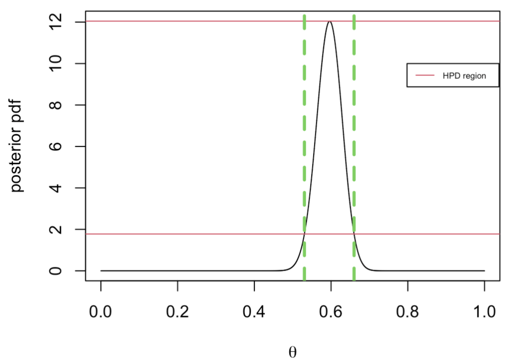
At the 18th-group data point, which is the ‘terminated’ data point for Case 1 with the uniform prior, we obtain the posterior distribution of $\theta \mid X_{218}\sim \mathrm{Beta}(131,89)$, where $X_{218}=130$. The calculated $95\%$ HPD region of $\theta$ is $(0.5305,0.6599)$, shown in Figure 5, which indicates that the corresponding $95\%$ HPD region of $\gamma$, the relative risk, is $(1.1298,1.9407)$. Note that the conditional Type I error probability is $0.1705$ for Case 1 under the modified Bayesian test. Although the $95\%$ HPD region excludes $\gamma =1$, the conditional Type I error probabilities indicate that there are around $17\%$ in favor of the null hypothesis for Case 1.

Figure 5. The $95\%$ HPD region of $\theta \mid X_{218}\sim \mathrm{Beta}(131,89)$ where $X_{218}=130$ at the 18th-group data point with the posterior $pdf$ of $\theta \mid X_{218}$ in Case 1.

At the 17th-group data point, which is the ‘terminated’ data point for Case 1 with the informative prior, we obtain the posterior distribution of $\theta \mid X_{211}\sim \mathrm{Beta}(237.8288,200.8288)$, where $X_{211}=124$. The calculated $95\%$ HPD region of $\theta$ is $(0.4955,0.5888)$, which indicates that the corresponding $95\%$ HPD region of $\gamma$ is $(0.9820,1.4318)$. Note that the conditional Type I error probability is $0.2249$ for Case 1 under the modified Bayesian test.

• Case 2 ($H_0^{(2)}:\gamma =1\mathbf{against}{H}_1^{(2)}:\gamma >1$)

At the 17th-group data point, which is the ‘terminated’ data point for Case 2 with the uniform prior, we obtain the posterior distribution of $\theta \mid X_{211}\sim \mathrm{Beta}(125,88)$, where $X_{211}=124$. The calculated $95\%$ HPD region of $\theta$ is $(0.4955,0.5888)$, which indicates the corresponding $95\%$ HPD region of $\gamma$, the relative risk, is $(0.9820,1.4318)$. Note that the conditional Type I error probability is $0.1855$ for Case 2 under the modified Bayesian test.

At the 16th-group data point, which is the ‘terminated’ data point for Case 2 with the informative prior, we obtain the posterior distribution of $\theta \mid X_{197}\sim \mathrm{Beta}(226.8288,197.8288)$, where $X_{197}=113$. The calculated $95\%$ HPD region of $\theta$ is $(0.4867,0.5815)$, which indicates that the corresponding $95\%$ HPD region of $\gamma$ is $(0.9483,1.3894)$. Note that the conditional Type I error probability is $0.2156$ for Case 2 under the modified Bayesian test.

• Case 3 ($H_0^{(3)}:\gamma \le 1\mathbf{against}{H}_1^{(3)}:\gamma >1$)

At the 14th-group data point, which is the ‘terminated’ data point for Case 3 with the uniform prior, we obtain the posterior distribution of $\theta \mid X_{172}\sim \mathrm{Beta}(92,82)$, where $X_{172}=91$. The calculated $95\%$ HPD region of $\theta$ is $(0.4546,0.6027)$, which indicates that the corresponding $95\%$ HPD region of $\gamma$ is $(0.8336,1.5168)$. The conditional Type I error probability is $0.2236$ under the modified Bayesian test.

At the 15th-group data point, which is the ‘terminated’ data point for Case 3 with the informative prior, we obtain the posterior distribution of $\theta \mid X_{190}\sim \mathrm{Beta}(220.8288,196.8288)$, where $X_{190}=107$. The calculated $95\%$ HPD region of $\theta$ is $(0.4809,0.5765)$, which indicates that the corresponding $95\%$ HPD region of $\gamma$ is $(0.9263,1.3613)$. The conditional Type I error probability is $0.1198$ under the modified Bayesian test.

Remark 3.

We notice that some $95\%$ HPD regions may include $\gamma =1$, the value of γ under the null hypothesis. Since the Bayes factor shows that the overall evidence from the data favors the alternative compared to the null, the $95\%$ HPD region reflects that the null is not entirely implausible. Even if the null value is within the $95\%$ HPD region, the posterior may still assign higher credibility to other values (those outside the null), which explains why the Bayes factor rejects the null. Hence, the null hypothesis may still be within a credible interval, but its likelihood is overshadowed by the alternative. It also indicates that the null hypothesis is rejected substantially.

3.4. Connection to the UMPBT

Considering Case 2, now treated as the UMPBT, we construct the corresponding ‘group’ sequential Bayesian test with a certain ‘termination’ point. However, we note that, in the current context, the threshold of the Bayes factor $B_m$ to reject the null hypothesis takes the form $B_m<1/\lambda$ for some $\lambda >0$. By Lemma 1 in ref. [6], the UMPBT($1/\lambda$) is constructed by finding ${\theta }_1$ that ${\theta }_1>{\theta }_0$ and

$${\theta }_1=arg\underset{\theta }{min}{\displaystyle \frac{ln(1/\lambda )-m\left[ln(1-\theta )-ln(1-{\theta }_0)\right]}{ln[\theta /(1-\theta )]-ln[{\theta }_0/(1-{\theta }_0)]}},$$

which can be solved numerically. For instance, by applying the suggestion of the Jeffrey’s evidence level shown in Table 2, we may reject the null hypothesis if $B_m<0.3162$, so that $1/\lambda =0.3162$ in this case.

(I)

Case of non-informative (uniform) prior distribution

Since the ‘termination’ point of Case 2 with the uniform prior is the 17th-group data point, we have $B_{211}=0.2278$ and $\text{Pr}(H_0^{(2)}\mid X_{211}=124)=0.1855$, $m=211$ and $X_m=124$. We use $1/\lambda =0.2059$ and obtain the corresponding ${\theta }_1=0.5611$. At this value of ${\theta }_1$ and ${\theta }_0=0.5$, $B_m<1/\lambda$ whenever 119 or more of the $n=211$ patients enrolled in this fixed sample size study. Accordingly, for the fixed-sample-size test (with $n=211$), once the number of the observed side effects was $X_n\ge 119$, we would reject the null hypothesis, incurring a (classical) Type I error probability $\alpha =P_{{\theta }_0}(X_n\ge 119)=0.0366$. The rejection region for this $3.66\%$ significance test also corresponds to the region for which the Bayes factor corresponding to the UMPBT($1/\lambda$) for all values of $1/\lambda \in (0.1775,0.2270)$. With equal prior probabilities of the null and the alternative hypotheses we assumed previously ($\ell =1$), the implied significant level of $0.0366$ for this UMPBT approximately corresponds to the Bayesian test, resulting in

$$0.1507<\text{Pr}(H_0^{(2)}\mid Data)<0.1850.$$

This serves as illustration of the fact that, unlike the posterior probabilities, the p-value or attained significant level is not a true measure of the strength of the evidence in favor/against the null hypothesis; see ref. [15] for a discussion of this point.

However, note that, if we choose Jeffrey’s evidence level of $1/\lambda =0.3162$, the calculated $B_{211}=0.3514$ and $\text{Pr}(H_0^{(2)}\mid X_{211}=124)=0.2600$, which would not match the results obtained from the UMPBT procedure in this case. This may be attributed to the group sequential nature of the data and the uniform prior that we considered here.

(II)

Case of informative prior distribution

Since the ‘termination’ point of Case 2 with the informative prior is the 16th-group data point, we have $B_{197}=0.2749$ and $\text{Pr}(H_0^{(2)}\mid X_{297}=113)=0.2156$, $m=197$ and $X_m=113$. Applying Jeffrey’s evidence level of $1/\lambda =0.3162$ with the corresponding (equivalent) fixed sample size of this UMPBT $n=197$, we obtain the corresponding ${\theta }_1=0.5540$. With these values of ${\theta }_1$ and ${\theta }_0=0.5$, $B_m<1/\lambda$ whenever 110 or more of the $n=197$ patients enrolled in this fixed sample size study. Accordingly, for the fixed-sample-size test, once the number of the observed side effects was $X_n\ge 110$, we would reject the null hypothesis, incurring a (classical) Type I error $\alpha =P_{{\theta }_0}(X_n\ge 110)=0.0584$. The rejection region for this $5.84\%$ significance test also corresponds to the region for which the Bayes factor corresponding to the UMPBT($1/\lambda$) for all values of $1/\lambda \in (0.2624,0.3259)$. With equal prior probabilities of the null and the alternative hypotheses we assumed previously ($\ell =1$), the implied significant level of $0.0584$ for this UMPBT, which approximately corresponds to the Bayesian test, resulted in

$$0.2078<\text{Pr}(H_0^{(2)}\mid Data)<0.2458.$$

3.5. Simulation Results

In this subsection, we provide the results of some simulations of Case 2 of $H_0^{(2)}$ and $H_1^{(2)}$ (see (15)), aimed at illustrating further the properties of the sequential Bayesian testing procedure. For the simulations, we utilize the method introduced in ref. [9] to simulate the values of the relevant stopping time $M^{*}$ for the corresponding $(\alpha ,\beta )$-UMP test of $H_0:$$\theta =1/2$ versus $H_1:$$\theta >1/2$, with an optimal sample size $N^{*}$, as was determined by $\alpha =0.05$ and $\beta =0.1$ for various alternative choices of $\theta$. Relation (1) for $\theta (\gamma )$ was then utilized to express these hypotheses in terms of the relative risk $\gamma$. The simulated values of the data, along with $M^{*}$, were then used to calculate the values of the Bayes factor $B_{M^{*}}$ in (16). Based on the standard shown in Table 2, $H_0$ would be rejected if the calculated $B_{M^{*}}<0.3162$. Throughout the 10,000 simulation runs, we assumed that the prior probability of $H_0$ is ${\pi }_0=1/2$. The results are presented in Table 9, which provide the calculated power and probability of the Type I error of the test for different sample sizes (different $N^{*}$) and different priors choices for $\theta$, as were used in the standard Bayesian test. To that end, we simulated the data under the alternative choices of $\gamma$ (equivalently of $\theta$) of $\gamma =1.5,\gamma =2,$ and $\gamma =1$ as well. As can be seen, as the sample size increases, the power increases as expected, regardless of the priors. Moreover, the Type I error probability decreases with the sample size under a uniform prior, but increases when the sample size increases under informative prior, which indicates that the Bayes factors may exhibit sensitivity to prior specification, giving support to default type choices for a prior distribution of $\theta$. One should also note that, when the value of the Bayes factor we calculated is much less than the critical value $0.3162$, the simulated value of Type I error probability is much less than the nominal value of $\alpha$ that we predefined for the UMP test.

Table 9. Power and Type I error probability of the standard Bayesian test for $\gamma =1.5,2$ in $H_1$ and $\gamma =1$ in $H_0$ of Case 2 for different sample sizes under different priors. ‘_avg’ indicates the average of the corresponding simulated values.

	uniform prior
	$\gamma =1.5$				$\gamma =2$				$\gamma =1$
$N^{*}$	power	${(B_{M^{*}})}_{avg}$	${(\text{Pr}(H_0^{(2)}\mid X_{M^{*}}))}_{avg}$		power	${(B_{M^{*}})}_{avg}$	${(\text{Pr}(H_0^{(2)}\mid X_{M^{*}}))}_{avg}$		$\alpha$	${(B_{M^{*}})}_{avg}$	${(\text{Pr}(H_0^{(2)}\mid X_{M^{*}}))}_{avg}$
210	0.6635	0.5656	0.2035		0.9921	0.0135	0.0103		0.0073	13.2014	0.8769
261	0.7813	0.3583	0.1456		0.9982	0.0041	0.0033		0.0081	14.6915	0.8859
331	0.8669	0.1952	0.0922		0.9998	0.0008	0.0007		0.0053	16.4740	0.8956
433	0.9407	0.0788	0.0443		1.0000	<0.0001	<0.0001		0.0047	18.8944	0.9047
591	0.9869	0.0206	0.0132		1.0000	<0.0001	<0.0001		0.0049	21.9616	0.9154
	informative prior
	$\gamma =1.5$				$\gamma =2$				$\gamma =1$
$N^{*}$	power	${(B_{M^{*}})}_{avg}$	${(\text{Pr}(H_0^{(2)}\mid X_{M^{*}}))}_{avg}$		power	${(B_{M^{*}})}_{avg}$	${(\text{Pr}(H_0^{(2)}\mid X_{M^{*}}))}_{avg}$		$\alpha$	${(B_{M^{*}})}_{avg}$	${(\text{Pr}(H_0^{(2)}\mid X_{M^{*}}))}_{avg}$
210	0.8488	0.1753	0.1312		0.9990	0.0210	0.0196		0.0277	1.4843	0.5594
261	0.9293	0.1116	0.0879		0.9999	0.0068	0.0065		0.0332	1.5776	0.5693
331	0.9682	0.0611	0.0508		1.0000	0.0014	0.0014		0.0321	1.6940	0.5812
433	0.9925	0.0249	0.0219		1.0000	0.0001	0.0001		0.0374	1.8608	0.5968
591	0.9990	0.0062	0.0057		1.0000	<0.0001	<0.0001		0.0391	2.0798	0.6162

The results from applying the Modified Bayesian Test in (22) for Case 2 with these choices of values of $\gamma$ and with $N^{*}=210$ are presented in Table 10. The values of r and u in (22) were obtained according to (23). As we can see, when $\gamma =1.5$, we have an $84.88\%$ chance to correctly reject $H_0$, with the average conditional Type I error probability being $0.1198$ under the uniform prior. Compared with the result shown in Table 9, when $\gamma =1.5$, we have a $66.35\%$ chance to correctly reject $H_0$, with the average posterior probability being $0.2035$ under the uniform prior. Moreover, we note that these simulations resulted in a $31.06\%$ chance to reject the null, a $58.85\%$ chance to accept the null, and a $10.09\%$ chance to conclude with no decision when $\gamma =1$ under the chosen informative prior. We attribute this particular outcome to the particular choice of the $(a,b)$ parameters of the prior distribution and the likely inadequacy of the sample size in this discrete case. To allow a comparison with an ‘objective-type’ of prior choice, we augmented the simulation study of the Uniform and the Informative type choices of priors, with the Jefferey’s prior for the Binomial case having $a=b=0.5$ (see Table 10). Clearly, further simulations are needed to explore the full spectrum of the potential sensitivity to the prior choices. However, for the sake of space, we leave that to future studies. To facilitate reproducibility, we provide the sample simulation code as Supplementary Material.

Table 10. Decision and the conditional error probability of Bayesian modified hypotheses test for $\gamma =1.5,2$ in $H_1$ and $\gamma =1$ in $H_0$ of Case 2 in sample size $N^{*}=210$ under different priors. ‘_avg’ indicates the average of the corresponding simulated values. ‘NA’ indicates No Answer.

	Uniform Prior			Jeffrey’s Prior			Informative Prior
$\mathit{\gamma }$	Decision		${\mathbf{(}{\mathit{\alpha }}^{\mathbf{*}}\mathbf{(}\mathbf{or}{\mathit{\beta }}^{\mathbf{*}}\mathbf{)}\mathbf{)}}_{\mathit{avg}}$	Decision		${\mathbf{(}{\mathit{\alpha }}^{\mathbf{*}}\mathbf{(}\mathbf{or}{\mathit{\beta }}^{\mathbf{*}}\mathbf{)}\mathbf{)}}_{\mathit{avg}}$	Decision		${\mathbf{(}{\mathit{\alpha }}^{\mathbf{*}}\mathbf{(}\mathbf{or}{\mathit{\beta }}^{\mathbf{*}}\mathbf{)}\mathbf{)}}_{\mathit{avg}}$
$1.5$	$84.88\%$	Rejection	0.1198	$80.66\%$	Rejection	0.1410	$99.27\%$	Rejection	0.1281
	$12.38\%$	No Decision	NA	14.60%	No Decision	NA	0.44%	No Decision	NA
	$2.74\%$	Acceptance	0.1461	$4.74\%$	Acceptance	0.1274	$0.29\%$	Acceptance	0.4033
2	$99.90\%$	Rejection	0.0097	$99.78\%$	Rejection	0.0132	$100.00\%$	Rejection	0.0196
	$0.09\%$	No Decision	NA	$0.19\%$	No Decision	NA
	$0.01\%$	Acceptance	0.2113	$0.03\%$	Acceptance	0.1607
1	$2.77\%$	Rejection	0.3053	$1.98\%$	Rejection	0.3293	$31.06\%$	Rejection	0.3945
	$11.79\%$	No Decision	NA	$7.86\%$	No Decision	NA	$10.09\%$	No Decision	NA
	$85.44\%$	Acceptance	0.0804	$90.16\%$	Acceptance	0.0591	$58.85\%$	Acceptance	0.3487

4. Summary and Discussion

In this paper, we propose the standard Bayesian test and the modified Bayesian test of hypotheses concerning the relative risk, $\gamma$, of a two-arm clinical trial. In this context, the relative risk $\gamma$ can be represented as $\theta (\gamma )$—a parameter representing an event probability. Since the output of each observation collected is binary data, the sequential experimental process can be viewed as a sequential binomial process with a probability of $\theta (\gamma )$. Note that, under the Bayesian framework, based on the SRP, each data point remains unaffected by the optimal stopping rule used in the process (unlike the ‘classical’ sequential test). Within the Bayesian framework, we consider the sequential testing of hypotheses concerning the parameter $\theta (\gamma )$. By utilizing the conjugate beta-binomial model, we are able to obtain the corresponding decision ‘rule’ for the test at each observed data point as determined from the calculated value of the Bayes factor.

To deal with the values of the Bayes factors that are too close to the decision boundaries, Jefferey’s criteria for the evidentiary level for a ‘rejection of $H_0$’ are taken into consideration. Additionally, we consider a modification of the standard Bayesian test ref. [5], which includes a ‘no-decision’ region, and calculate the corresponding conditional Type I and Type II error probabilities ${\alpha }^{*}$ and ${\beta }^{*}$. To illustrate our approach and the methods discussed, we analyze the data presented in ref. [2] under the three different hypothesis testing cases and several different priors. It is worth pointing out that the informative prior we propose is designed to use the knowledge of the bounded-width probability. For each case with different priors, we analyze the calculated Bayes factor corresponding to each data point and make the decision within two Bayesian tests.

Specifically, we consider, in Case 2, the very same hypothesis testing problem as shown in ref. [2]. The result presented in ref. [2] indicates that the testing procedure should have been terminated at the 19th-group data point. However, the results obtained from the standard Bayesian test and the modified Bayesian test lead to a potentially earlier ‘termination’ at the 17th-group data point under the uniform prior and at the 16th-group data point under an informative prior. Furthermore, utilizing the modified Bayesian test with a uniform prior, at the 17th-group data point, the Type I error conditional probability is ${\alpha }^{*}=0.1855$ (given the data). Similarly, with the modified Bayesian test and under an informative prior, at the 16th-group data point, the conditional Type I error probability is ${\alpha }^{*}=0.2156$ (given the data). From Section 3.4, we find our ‘termination’ based on the Bayesian test with a uniform prior corresponding to a p-value of $0.0366$ and with an informative prior corresponding to a p-value of $0.0584$ from the frequentist point of view.

Case 3 has the very same hypothesis testing problem as shown in ref. [3]. The result presented in ref. [3] indicates that the testing procedure should have been terminated at the 18th-group data point. However, the results obtained from both the standard Bayesian test and the modified Bayesian test lead to the potentially earlier ‘termination’ at the 14th-group data point with a uniform prior and at the 15th-group data point with an informative prior. Furthermore, with the modified Bayesian test under a uniform prior, at the 14th-group data point, the conditional Type I error probability ${\alpha }^{*}=0.2236$ (given the data). Similarly, with the modified Bayesian test under an informative prior, at the 15th-group data point, the conditional Type I error probability is ${\alpha }^{*}=0.1198$ (given the data).

These cases illustrate the benefits of Bayesian testing in this context. Unlike the classical sequential test, which typically requires heavy calculations to determine ‘stopping boundaries’ as well as ‘decision boundaries’ (for a-priory specified Type I and Type II error probabilities), the Bayesian test is easy to use and implement, and it could obtain the test results in a relatively simple manner. Compared with the results obtained in refs. [2,3], we conclude that our results are consistent with their results. Although our decisions for Case 2 and Case 3 arrive slightly earlier than theirs, the values of the data points are similar.

Clearly, our Bayesian approach, which allows for a posterior-based analysis (as well as interpretations) of the available data as was collected, is simpler and, one could argue, more intuitive. It is attractive to those who prescribe to implementing the Bayesian paradigm, especially in clinical studies, where expert opinion and prior information is amply available. However, to others, the Bayesian framework and the testing procedure we advocate for here could potentially be seen as particularly limiting. The potential dependency on the choice of the prior distribution of the relevant parameters, the inclusion of the no-decision region as part of the terminal testing procedure, and the interpretation of the posterior measure of evidence could all seen as limitations to the practitioner. The reader may find the Discussion and the Rejoinder parts of ref. [5] as valuable resources for these considerations, as well as ref. [16] as a resource for a general discussion concerning the applicability of the Modified Bayesian test and the no-decision region in sequential clinical trail settings.

In addition, we are able to illustrate, using the very same data, the connection of our Bayesian test and the UMPBT. With this connection, the results we obtained from the Bayesian test can be approximately interpreted by the rejection region and the p-value from the frequentist perspective of the UMP. Moreover, by applying the modified Bayesian test, we could even obtain conditional error probabilities as well, which give us a measure of the data evidence in making decisions (of ‘Reject’ $H_0$ or ‘Accept’ $H_0$). Indeed, for such binary data hypothesis testing, utilizing Bayesian framework could provide a straightforward and easy path to analyze the data.

Appendix A.1. The Standard Bayesian Test

Introduced in ref. [14], the Jeffrey’s prior, as considered an ‘objective’ or non-informative prior distribution, is $\mathrm{Beta}(1/2,1/2)$ for binomial distributions in our case. We calculated the Bayes factor $B_m^{(i)}$ and the corresponding posterior probability $\text{Pr}(H_0^{(i)}\mid X_m=x)$, $i=1,2,3$ for the hypotheses tests on the RR, $\gamma$, in the three cases we considered. The numerical results are provided in Table A1 below.

As can be seen, for the hypotheses of Case 1 and Cse 2, our Bayesian model led to the potentially earlier ‘termination’ at the 18th-group data point with a total of $m=218$ ‘events’, the observed side effects of which $X_m=130$ were noted in the treatment group with an estimated relative risk of $\widehat{\gamma }=X_m/(m-X_m)=1.4773$. The resulting Bayes factors are $B_{218}^{(1)}=0.3160$ in Case 1 and $B_{218}^{(2)}=0.1583$ in Case 2, which is less than $0.3162$ based on the standard shown in Table 2. This leads to a rejection of $H_0^{(i)}$, $i=1,2$, and the posterior probabilities of the null hypothesis and the alternative hypothesis given the data are

$$\text{Pr}(H_0^{(1)}:\gamma =1\mid X_{218}=130)=0.2401\text{Pr}(H_1^{(1)}:\gamma \ne 1\mid X_{218}=130)=0.7599,$$

$$\text{Pr}(H_0^{(2)}:\gamma =1\mid X_{218}=130)=0.1367\text{Pr}(H_1^{(2)}:\gamma >1\mid X_{218}=130)=0.8633,$$

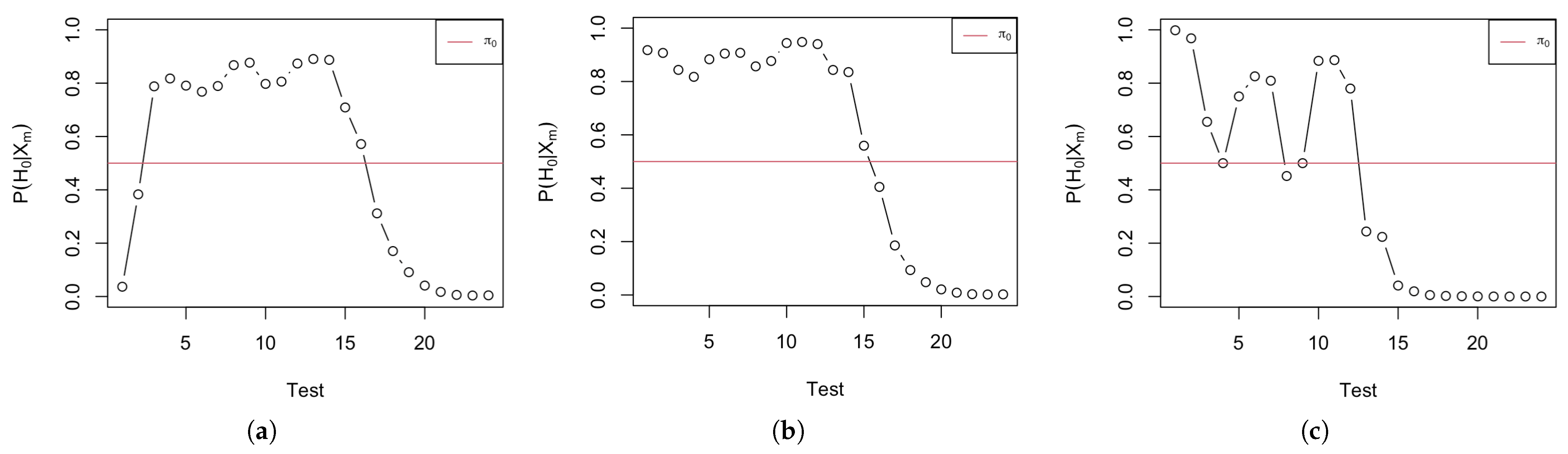
which are clearly smaller than the assumed prior probability ${\pi }_0=0.5$ of $H_0^{(i)}$, $i=1,2$ being true (marked in a red line in Figure A1).

On the other hand, for the hypotheses of Case 3, the observation process would ‘terminate’ much earlier at the 14th-group data point with a total of $m=172$ ‘events’, the observed side effects of which $X_m=91$ were noted in the treatment group, leading to the estimated relative risk of $\widehat{\gamma }=X_m/(m-X_m)=1.1235$. The resulting Bayes factor is $B_{172}^{(3)}=0.2869$, which is less than $0.3162$ based on the standard shown in Table 2, and the posterior probabilities of the null hypothesis and the alternative hypothesis given the data are

$$\text{Pr}(H_0^{(3)}:\gamma \le 1\mid X_{172}=91)=0.2229\mathrm{and}\text{Pr}(H_1^{(3)}:\gamma >1\mid X_{172}=91)=0.7771,$$

which are clearly smaller than the assumed prior probability ${\pi }_0=0.5$ of $H_0^{(3)}$ being true (marked in a red line in Figure A1).

Figure A1. The posterior probability of $H_0$ for the 24 data points of Table A1: (a) Case 1; (b) Case 2; (c) Case 3.

Figure A1. The posterior probability of $H_0$ for the 24 data points of Table A1: (a) Case 1; (b) Case 2; (c) Case 3.

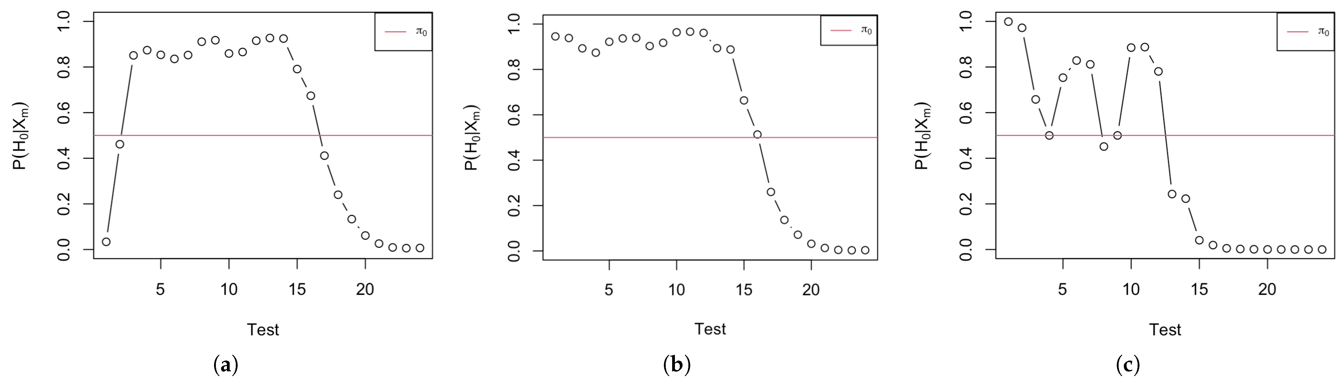
Table A1. The values of Bayes factor and posterior probability of $H_0$ for each data point among the three different cases with the Jeffrey’s prior.

Test	m	${\mathit{X}}_{\mathit{m}}$	$\widehat{\mathit{\gamma }}$	${\mathit{B}}_{\mathit{m}}^{(1)}$	$\text{Pr}({\mathit{H}}_0^{(1)}\mid {\mathit{X}}_{\mathit{m}})$	${\mathit{B}}_{\mathit{m}}^{(2)}$	$\text{Pr}({\mathit{H}}_0^{(2)}\mid {\mathit{X}}_{\mathit{m}})$	${\mathit{B}}_{\mathit{m}}^{(3)}$	$\text{Pr}({\mathit{H}}_0^{(3)}\mid {\mathit{X}}_{\mathit{m}})$
1	12	1	0.0909	0.0348	0.0337	17.3919	0.9456	997.4399	0.9990
2	18	5	0.3846	0.8570	0.4615	15.2343	0.9384	34.5543	0.9719
3	24	11	0.8462	5.7079	0.8509	8.3446	0.8930	1.9239	0.6580
4	30	15	1.0000	6.9221	0.8738	6.9221	0.8738	1.0000	0.5000
5	34	15	0.7895	5.8156	0.8533	11.7887	0.9218	3.0541	0.7533
6	40	17	0.7391	5.0778	0.8355	14.8076	0.9367	4.8323	0.8285
7	46	20	0.7692	5.7730	0.8524	15.3309	0.9388	4.3113	0.8117
8	67	34	1.0303	10.2206	0.9109	9.3159	0.9031	0.8230	0.4514
9	78	39	1.0000	11.1045	0.9174	11.1045	0.9174	1.0000	0.5000
10	100	44	0.7857	6.1053	0.8593	26.5481	0.9637	7.6967	0.8850
11	115	51	0.7969	6.4501	0.8658	28.6341	0.9663	7.8787	0.8874
12	135	63	0.8750	10.8056	0.9153	24.6313	0.9610	3.5590	0.7807
13	167	88	1.1139	12.7261	0.9271	8.4071	0.8937	0.3212	0.2431
14	172	91	1.1235	12.3066	0.9248	7.9186	0.8879	0.2869	0.2229
15	190	107	1.2892	3.7840	0.7910	1.9723	0.6636	0.0424	0.0407
16	197	113	1.3452	2.0676	0.6740	1.0541	0.5132	0.0196	0.0193
17	211	124	1.4253	0.6991	0.4114	0.3514	0.2600	0.0054	0.0053
18	218	130	1.4773	0.3160	0.2401	0.1583	0.1367	0.0022	0.0022
19	222	134	1.5227	0.1538	0.1333	0.0770	0.0715	0.0010	0.0010
20	231	141	1.5667	0.0653	0.0613	0.0327	0.0316	0.0004	0.0004
21	240	148	1.6087	0.0266	0.0259	0.0133	0.0131	0.0001	0.0001
22	245	153	1.6630	0.0091	0.0090	0.0046	0.0045	0.0000	0.0000
23	247	155	1.6848	0.0058	0.0058	0.0029	0.0029	0.0000	0.0000
24	251	157	1.6702	0.0067	0.0067	0.0034	0.0034	0.0000	0.0000

Table A1. The values of Bayes factor and posterior probability of $H_0$ for each data point among the three different cases with the Jeffrey’s prior.

Test	m	${\mathit{X}}_{\mathit{m}}$	$\widehat{\mathit{\gamma }}$	${\mathit{B}}_{\mathit{m}}^{(1)}$	$\text{Pr}({\mathit{H}}_0^{(1)}\mid {\mathit{X}}_{\mathit{m}})$	${\mathit{B}}_{\mathit{m}}^{(2)}$	$\text{Pr}({\mathit{H}}_0^{(2)}\mid {\mathit{X}}_{\mathit{m}})$	${\mathit{B}}_{\mathit{m}}^{(3)}$	$\text{Pr}({\mathit{H}}_0^{(3)}\mid {\mathit{X}}_{\mathit{m}})$
1	12	1	0.0909	0.0348	0.0337	17.3919	0.9456	997.4399	0.9990
2	18	5	0.3846	0.8570	0.4615	15.2343	0.9384	34.5543	0.9719
3	24	11	0.8462	5.7079	0.8509	8.3446	0.8930	1.9239	0.6580
4	30	15	1.0000	6.9221	0.8738	6.9221	0.8738	1.0000	0.5000
5	34	15	0.7895	5.8156	0.8533	11.7887	0.9218	3.0541	0.7533
6	40	17	0.7391	5.0778	0.8355	14.8076	0.9367	4.8323	0.8285
7	46	20	0.7692	5.7730	0.8524	15.3309	0.9388	4.3113	0.8117
8	67	34	1.0303	10.2206	0.9109	9.3159	0.9031	0.8230	0.4514
9	78	39	1.0000	11.1045	0.9174	11.1045	0.9174	1.0000	0.5000
10	100	44	0.7857	6.1053	0.8593	26.5481	0.9637	7.6967	0.8850
11	115	51	0.7969	6.4501	0.8658	28.6341	0.9663	7.8787	0.8874
12	135	63	0.8750	10.8056	0.9153	24.6313	0.9610	3.5590	0.7807
13	167	88	1.1139	12.7261	0.9271	8.4071	0.8937	0.3212	0.2431
14	172	91	1.1235	12.3066	0.9248	7.9186	0.8879	0.2869	0.2229
15	190	107	1.2892	3.7840	0.7910	1.9723	0.6636	0.0424	0.0407
16	197	113	1.3452	2.0676	0.6740	1.0541	0.5132	0.0196	0.0193
17	211	124	1.4253	0.6991	0.4114	0.3514	0.2600	0.0054	0.0053
18	218	130	1.4773	0.3160	0.2401	0.1583	0.1367	0.0022	0.0022
19	222	134	1.5227	0.1538	0.1333	0.0770	0.0715	0.0010	0.0010
20	231	141	1.5667	0.0653	0.0613	0.0327	0.0316	0.0004	0.0004
21	240	148	1.6087	0.0266	0.0259	0.0133	0.0131	0.0001	0.0001
22	245	153	1.6630	0.0091	0.0090	0.0046	0.0045	0.0000	0.0000
23	247	155	1.6848	0.0058	0.0058	0.0029	0.0029	0.0000	0.0000
24	251	157	1.6702	0.0067	0.0067	0.0034	0.0034	0.0000	0.0000

In conclusion, under Jeffrey’s prior, both Case 1 and Case 2 would reject and be ‘terminated’ at the 18th-group data point, and Case 3 would reject and ‘terminated’ at the 14th-group data point.

Appendix A.2. The Modified Bayesian Test

In the modified Bayesian Sequential test, we obtain the same conclusions that were obtained utilizing the standard Bayesian test for the hypotheses $H_0^{(i)}$, $i=1,2,3$ (see Appendix A.1). The results corresponding to the Jeffrey’s prior distribution are shown in Figure A2, Table A2 and Table A3. The calculated conditional Type I and Type II error probabilities, ${\alpha }^{*}$ and ${\beta }^{*}$, corresponding to the ‘Reject’ or ‘Accept’ decision (see Table A3).

Figure A2. The acceptance and rejection boundaries of $B_m$ for the 24 data points of Table A2: (a) Case 1; (b) Case 2; (c) Case 3.

Figure A2. The acceptance and rejection boundaries of $B_m$ for the 24 data points of Table A2: (a) Case 1; (b) Case 2; (c) Case 3.

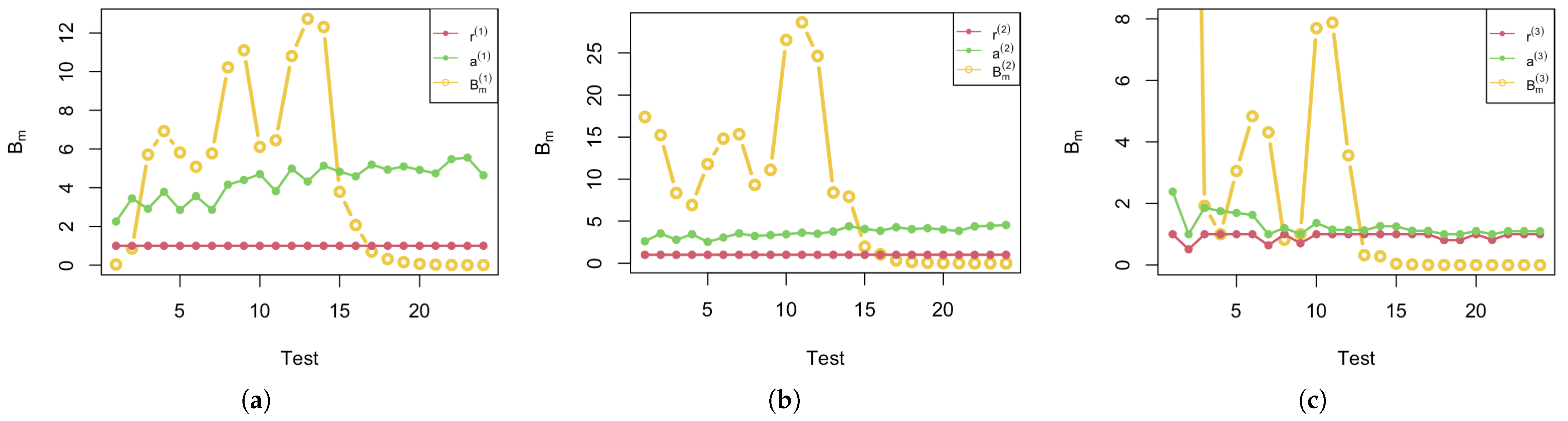
Table A2. The values of the Bayes factor and the boundaries based on it for each data point among different cases with Jeffrey’s prior.

Test	m	${\mathit{X}}_{\mathit{m}}$	$\widehat{\mathit{\gamma }}$	${\mathit{B}}_{\mathit{m}}^{(1)}$	${\mathit{r}}^{(1)}$	${\mathit{u}}^{(1)}$	${\mathit{B}}_{\mathit{m}}^{(2)}$	${\mathit{r}}^{(2)}$	${\mathit{u}}^{(2)}$	${\mathit{B}}_{\mathit{m}}^{(3)}$	${\mathit{r}}^{(3)}$	${\mathit{u}}^{(3)}$
1	12	1	0.0909	0.0348	1	2.2505	17.3919	1	2.6154	997.4399	1	2.3824
2	18	5	0.3846	0.8570	1	3.4458	15.2343	1	3.5437	34.5543	0.5104	1
3	24	11	0.8462	5.7079	1	2.9086	8.3446	1	2.8007	1.9239	1	1.8636
4	30	15	1.0000	6.9221	1	3.7844	6.9221	1	3.4535	1.0000	1	1.7492
5	34	15	0.7895	5.8156	1	2.8478	11.7887	1	2.5490	3.0541	1	1.6929
6	40	17	0.7391	5.0778	1	3.5652	14.8076	1	3.0643	4.8323	1	1.6267
7	46	20	0.7692	5.7730	1	2.8578	15.3309	1	3.5560	4.3113	0.6408	1
8	67	34	1.0303	10.2206	1	4.1572	9.3159	1	3.2489	0.8230	1	1.2029
9	78	39	1.0000	11.1045	1	4.3958	11.1045	1	3.3508	1.0000	0.7064	1
10	100	44	0.7857	6.1053	1	4.7006	26.5481	1	3.4493	7.6967	1	1.3656
11	115	51	0.7969	6.4501	1	3.8165	28.6341	1	3.6344	7.8787	1	1.1532
12	135	63	0.8750	10.8056	1	4.9882	24.6313	1	3.5097	3.5590	1	1.1411
13	167	88	1.1139	12.7261	1	4.3165	8.4071	1	3.7629	0.3212	1	1.1266
14	172	91	1.1235	12.3066	1	5.1324	7.9186	1	4.3949	0.2869	1	1.2698
15	190	107	1.2892	3.7840	1	4.8263	1.9723	1	4.0723	0.0424	1	1.2555
16	197	113	1.3452	2.0676	1	4.5858	1.0541	1	3.8566	0.0196	1	1.1163
17	211	124	1.4253	0.6991	1	5.1907	0.3514	1	4.2776	0.0054	1	1.1123
18	218	130	1.4773	0.3160	1	4.9304	0.1583	1	4.0516	0.0022	0.8092	1
19	222	134	1.5227	0.1538	1	5.0959	0.0770	1	4.1660	0.0010	0.8107	1
20	231	141	1.5667	0.0653	1	4.9166	0.0327	1	3.9997	0.0004	1	1.1072
21	240	148	1.6087	0.0266	1	4.7401	0.0133	1	3.8388	0.0001	0.8171	1
22	245	153	1.6630	0.0091	1	5.4724	0.0046	1	4.3810	0.0000	1	1.1040
23	247	155	1.6848	0.0058	1	5.5520	0.0029	1	4.4354	0.0000	1	1.1036
24	251	157	1.6702	0.0067	1	4.6391	0.0034	1	4.5442	0.0000	1	1.1027

Table A2. The values of the Bayes factor and the boundaries based on it for each data point among different cases with Jeffrey’s prior.

Test	m	${\mathit{X}}_{\mathit{m}}$	$\widehat{\mathit{\gamma }}$	${\mathit{B}}_{\mathit{m}}^{(1)}$	${\mathit{r}}^{(1)}$	${\mathit{u}}^{(1)}$	${\mathit{B}}_{\mathit{m}}^{(2)}$	${\mathit{r}}^{(2)}$	${\mathit{u}}^{(2)}$	${\mathit{B}}_{\mathit{m}}^{(3)}$	${\mathit{r}}^{(3)}$	${\mathit{u}}^{(3)}$
1	12	1	0.0909	0.0348	1	2.2505	17.3919	1	2.6154	997.4399	1	2.3824
2	18	5	0.3846	0.8570	1	3.4458	15.2343	1	3.5437	34.5543	0.5104	1
3	24	11	0.8462	5.7079	1	2.9086	8.3446	1	2.8007	1.9239	1	1.8636
4	30	15	1.0000	6.9221	1	3.7844	6.9221	1	3.4535	1.0000	1	1.7492
5	34	15	0.7895	5.8156	1	2.8478	11.7887	1	2.5490	3.0541	1	1.6929
6	40	17	0.7391	5.0778	1	3.5652	14.8076	1	3.0643	4.8323	1	1.6267
7	46	20	0.7692	5.7730	1	2.8578	15.3309	1	3.5560	4.3113	0.6408	1
8	67	34	1.0303	10.2206	1	4.1572	9.3159	1	3.2489	0.8230	1	1.2029
9	78	39	1.0000	11.1045	1	4.3958	11.1045	1	3.3508	1.0000	0.7064	1
10	100	44	0.7857	6.1053	1	4.7006	26.5481	1	3.4493	7.6967	1	1.3656
11	115	51	0.7969	6.4501	1	3.8165	28.6341	1	3.6344	7.8787	1	1.1532
12	135	63	0.8750	10.8056	1	4.9882	24.6313	1	3.5097	3.5590	1	1.1411
13	167	88	1.1139	12.7261	1	4.3165	8.4071	1	3.7629	0.3212	1	1.1266
14	172	91	1.1235	12.3066	1	5.1324	7.9186	1	4.3949	0.2869	1	1.2698
15	190	107	1.2892	3.7840	1	4.8263	1.9723	1	4.0723	0.0424	1	1.2555
16	197	113	1.3452	2.0676	1	4.5858	1.0541	1	3.8566	0.0196	1	1.1163
17	211	124	1.4253	0.6991	1	5.1907	0.3514	1	4.2776	0.0054	1	1.1123
18	218	130	1.4773	0.3160	1	4.9304	0.1583	1	4.0516	0.0022	0.8092	1
19	222	134	1.5227	0.1538	1	5.0959	0.0770	1	4.1660	0.0010	0.8107	1
20	231	141	1.5667	0.0653	1	4.9166	0.0327	1	3.9997	0.0004	1	1.1072
21	240	148	1.6087	0.0266	1	4.7401	0.0133	1	3.8388	0.0001	0.8171	1
22	245	153	1.6630	0.0091	1	5.4724	0.0046	1	4.3810	0.0000	1	1.1040
23	247	155	1.6848	0.0058	1	5.5520	0.0029	1	4.4354	0.0000	1	1.1036
24	251	157	1.6702	0.0067	1	4.6391	0.0034	1	4.5442	0.0000	1	1.1027

Table A3. The decision and corresponding conditional ${\alpha }^{*}$ and ${\beta }^{*}$ for each data point among different cases with Jeffrey’s prior (Decision: ‘R’ indicates Reject, ‘A’ indicates Accept, ‘ND’ indicates No Decision, ‘NA’ indicates No Answer).

Test	$\widehat{\mathit{\gamma }}$	${\mathit{B}}_{\mathit{m}}^{(1)}$	Decision	${\mathit{\alpha }}^{*}(\mathbf{or}{\mathit{\beta }}^{*})$	${\mathit{B}}_{\mathit{m}}^{(2)}$	Decision	${\mathit{\alpha }}^{*}(\mathbf{or}{\mathit{\beta }}^{*})$	${\mathit{B}}_{\mathit{m}}^{(3)}$	Decision	${\mathit{\alpha }}^{*}(\mathbf{or}{\mathit{\beta }}^{*})$
1	0.0909	0.0348	R	0.0336	17.3919	A	0.0556	997.4399	A	0.0010
2	0.3846	0.8570	R	0.4615	15.2343	A	0.0619	34.5543	A	0.0256
3	0.8462	5.7079	A	0.1773	8.3446	A	0.1154	1.9239	A	0.3304
4	1.0000	6.9221	A	0.1263	6.9221	A	0.1332	1.0000	ND	NA
5	0.7895	5.8156	A	0.1490	11.7887	A	0.0883	3.0541	A	0.2449
6	0.7391	5.0778	A	0.1773	14.8076	A	0.0693	4.8323	A	0.1427
7	0.7692	5.7730	A	0.1490	15.3309	A	0.0619	4.3113	A	0.1730
8	1.0303	10.2206	A	0.0937	9.3159	A	0.1006	0.8230	R	0.4515
9	1.0000	11.1045	A	0.0937	11.1045	A	0.0883	1.0000	ND	NA
10	0.7857	6.1053	A	0.1490	26.5481	A	0.0383	7.6967	A	0.0934
11	0.7969	6.4501	A	0.1490	28.6341	A	0.0353	7.8787	A	0.0934
12	0.8750	10.8056	A	0.0937	24.6313	A	0.0417	3.5590	A	0.2071
13	1.1139	12.7261	A	0.0730	8.4071	A	0.1154	0.3212	R	0.2431
14	1.1235	12.3066	A	0.0821	7.9186	A	0.1154	0.2869	R	0.2229
15	1.2892	3.7840	ND	NA	1.9723	ND	NA	0.0424	R	0.0407
16	1.3452	2.0676	ND	NA	1.0541	ND	NA	0.0196	R	0.0192
17	1.4253	0.6991	R	0.4115	0.3514	R	0.2600	0.0054	R	0.0054
18	1.4773	0.3160	R	0.2401	0.1583	R	0.1367	0.0022	R	0.0022
19	1.5227	0.1538	R	0.1333	0.0770	R	0.0715	0.0010	R	0.0010
20	1.5667	0.0653	R	0.0613	0.0327	R	0.0317	0.0004	R	0.0004
21	1.6087	0.0266	R	0.0259	0.0133	R	0.0131	0.0001	R	0.0001
22	1.6630	0.0091	R	0.0090	0.0046	R	0.0046	0.0000	R	0.0000
23	1.6848	0.0058	R	0.0058	0.0029	R	0.0029	0.0000	R	0.0000
24	1.6702	0.0067	R	0.0067	0.0034	R	0.0034	0.0000	R	0.0000

Table A3. The decision and corresponding conditional ${\alpha }^{*}$ and ${\beta }^{*}$ for each data point among different cases with Jeffrey’s prior (Decision: ‘R’ indicates Reject, ‘A’ indicates Accept, ‘ND’ indicates No Decision, ‘NA’ indicates No Answer).

Test	$\widehat{\mathit{\gamma }}$	${\mathit{B}}_{\mathit{m}}^{(1)}$	Decision	${\mathit{\alpha }}^{*}(\mathbf{or}{\mathit{\beta }}^{*})$	${\mathit{B}}_{\mathit{m}}^{(2)}$	Decision	${\mathit{\alpha }}^{*}(\mathbf{or}{\mathit{\beta }}^{*})$	${\mathit{B}}_{\mathit{m}}^{(3)}$	Decision	${\mathit{\alpha }}^{*}(\mathbf{or}{\mathit{\beta }}^{*})$
1	0.0909	0.0348	R	0.0336	17.3919	A	0.0556	997.4399	A	0.0010
2	0.3846	0.8570	R	0.4615	15.2343	A	0.0619	34.5543	A	0.0256
3	0.8462	5.7079	A	0.1773	8.3446	A	0.1154	1.9239	A	0.3304
4	1.0000	6.9221	A	0.1263	6.9221	A	0.1332	1.0000	ND	NA
5	0.7895	5.8156	A	0.1490	11.7887	A	0.0883	3.0541	A	0.2449
6	0.7391	5.0778	A	0.1773	14.8076	A	0.0693	4.8323	A	0.1427
7	0.7692	5.7730	A	0.1490	15.3309	A	0.0619	4.3113	A	0.1730
8	1.0303	10.2206	A	0.0937	9.3159	A	0.1006	0.8230	R	0.4515
9	1.0000	11.1045	A	0.0937	11.1045	A	0.0883	1.0000	ND	NA
10	0.7857	6.1053	A	0.1490	26.5481	A	0.0383	7.6967	A	0.0934
11	0.7969	6.4501	A	0.1490	28.6341	A	0.0353	7.8787	A	0.0934
12	0.8750	10.8056	A	0.0937	24.6313	A	0.0417	3.5590	A	0.2071
13	1.1139	12.7261	A	0.0730	8.4071	A	0.1154	0.3212	R	0.2431
14	1.1235	12.3066	A	0.0821	7.9186	A	0.1154	0.2869	R	0.2229
15	1.2892	3.7840	ND	NA	1.9723	ND	NA	0.0424	R	0.0407
16	1.3452	2.0676	ND	NA	1.0541	ND	NA	0.0196	R	0.0192
17	1.4253	0.6991	R	0.4115	0.3514	R	0.2600	0.0054	R	0.0054
18	1.4773	0.3160	R	0.2401	0.1583	R	0.1367	0.0022	R	0.0022
19	1.5227	0.1538	R	0.1333	0.0770	R	0.0715	0.0010	R	0.0010
20	1.5667	0.0653	R	0.0613	0.0327	R	0.0317	0.0004	R	0.0004
21	1.6087	0.0266	R	0.0259	0.0133	R	0.0131	0.0001	R	0.0001
22	1.6630	0.0091	R	0.0090	0.0046	R	0.0046	0.0000	R	0.0000
23	1.6848	0.0058	R	0.0058	0.0029	R	0.0029	0.0000	R	0.0000
24	1.6702	0.0067	R	0.0067	0.0034	R	0.0034	0.0000	R	0.0000

References

- Lee, G.M.; Greene, S.K.; Weintraub, E.S.; Baggs, J.; Kulldorff, M.; Fireman, B.H.; Baxter, R.; Jacobsen, S.J.; Irving, S.; Daley, M.F.; et al. H1N1 and seasonal influenza vaccine safety in the vaccine safety datalink project. Am. J. Prev. Med. 2011, 41, 121–128. [Google Scholar] [CrossRef] [Scilit] [PubMed]
- Silva, I.R.; Kulldorff, M.; Katherine Yih, W. Optimal alpha spending for sequential analysis with binomial data. J. R. Stat. Soc. Ser. B Stat. Methodol. 2020, 82, 1141–1164. [Google Scholar] [CrossRef] [Scilit]
- Silva, I.R.; Zhuang, Y. Bounded-width confidence interval following optimal sequential analysis of adverse events with binary data. Stat. Methods Med. Res. 2022, 31, 2323–2337. [Google Scholar] [CrossRef] [Scilit] [PubMed]
- Berger, J.O.; Wolpert, R.L. The Likelihood Principle; IMS: Waite Hill, OH, USA, 1988. [Google Scholar]
- Berger, J.O.; Boukai, B.; Wang, Y. Unified frequentist and Bayesian testing of a precise hypothesis. Stat. Sci. 1997, 12, 133–160. [Google Scholar] [CrossRef] [Scilit]
- Johnson, V.E. Uniformly most powerful Bayesian tests. Ann. Stat. 2013, 41, 1716. [Google Scholar] [CrossRef] [Scilit] [PubMed]
- Nikooienejad, A.; Johnson, V.E. On the existence of uniformly most powerful bayesian tests with application to non-central chi-squared tests. Bayesian Anal. 2021, 16, 93. [Google Scholar] [CrossRef] [Scilit] [PubMed]
- Silva, I.R.; Maro, J.; Kulldorff, M. Exact sequential test for clinical trials and post-market drug and vaccine safety surveillance with Poisson and binary data. Stat. Med. 2021, 40, 4890–4913. [Google Scholar] [CrossRef] [Scilit] [PubMed]
- Wang, J.; Boukai, B. Early detection of treatment’s acute side effect: A sequential approach: J. Wang, B. Boukai. Stat. Pap. 2026, 67, 22. [Google Scholar] [CrossRef] [Scilit]
- Kulldorff, M.; Davis, R.L.; Kolczak, M.; Lewis, E.; Lieu, T.; Platt, R. A maximized sequential probability ratio test for drug and vaccine safety surveillance. Seq. Anal. 2011, 30, 58–78. [Google Scholar] [CrossRef] [Scilit]
- Jeffreys, H. Theory of Probability, 3rd ed.; Clarendon Press: Oxford, UK, 1961. [Google Scholar]
- Kass, R.E.; Raftery, A.E. Bayes factors. J. Am. Stat. Assoc. 1995, 90, 773–795. [Google Scholar] [CrossRef]
- Berger, J.O. Statistical Decision Theory and Bayesian Analysis; Springer Science & Business Media: New York, NY, USA, 2013. [Google Scholar]
- Jeffreys, H. An invariant form for the prior probability in estimation problems. Proc. R. Soc. Lond. Ser. A Math. Phys. Sci. 1946, 186, 453–461. [Google Scholar] [CrossRef] [Scilit]
- Sellke, T.; Bayarri, M.J.; Berger, J.O. Calibration of ρ values for testing precise null hypotheses. Am. Stat. 2001, 55, 62–71. [Google Scholar] [CrossRef] [Scilit]
- Berger, J.O.; Boukai, B.; Wang, Y. Simultaneous Bayesian-frequentist sequential testing of nested hypotheses. Biometrika 1999, 86, 79–92. [Google Scholar] [CrossRef] [Scilit]
Disclaimer/Publisher’s Note: The statements, opinions and data contained in all publications are solely those of the individual author(s) and contributor(s) and not of MDPI and/or the editor(s). MDPI and/or the editor(s) disclaim responsibility for any injury to people or property resulting from any ideas, methods, instructions or products referred to in the content. |
© 2026 by the authors. Licensee MDPI, Basel, Switzerland. This article is an open access article distributed under the terms and conditions of the Creative Commons Attribution (CC BY) license.