


Abstract
Carbonation in CO2-storage solid-waste backfill materials couples CO2 transport, mineral reaction, and strength evolution, making carbonation-front prediction and transport–reaction inference important for evaluating sequestration performance. This study proposes an evidence-ranked, physics-guided inverse-learning framework for carbonation-front prediction, auxiliary strength reconstruction, PDE-residual assessment, and practical-identifiability analysis. The framework represents carbonation using group-conditioned latent fields of effective CO2 concentration and remaining reactive capacity, maps latent carbonation degree to measured depth through a differentiable front operator, and reconstructs unconfined compressive strength through a supervised auxiliary head. Empirical front laws and reaction–diffusion physics-informed neural-network variants were evaluated using held-out ranking, repeated stratified splits, residual-weight sweeps, front-operator threshold and smoothing-coefficient sensitivity checks, profile-likelihood and Fisher-information diagnostics, and controlled synthetic tests. Results show that the grouped Weibull front law achieved the best short-range carbonation-depth interpolation, while the retained constant-diffusion PINN was used as a diagnostic formulation within the physics-guided family to improve auxiliary strength reconstruction and to evaluate residual consistency, front-threshold selection, parameter sharing, and inverse-parameter behavior rather than to replace the empirical depth regressor. Increasing the PDE-residual weight substantially reduced residual magnitudes, but profile-likelihood and Fisher-information diagnostics indicated strong parameter trade-offs; the fitted diffusion, reaction, depletion, and diffusion–decay quantities are therefore interpreted as effective, observation-conditional parameters rather than unique material constants. The proposed framework provides a prediction-first and attribution-aware approach for analyzing carbonation evolution in solid-waste backfill materials and supports coordinated assessment of front advancement, strength response, and transport–reaction behavior, while explicitly delimiting the generalization and physical interpretation that can be supported by sparse literature-derived observations.
Keywords:
carbonation depth; reaction–diffusion; inverse modeling; physics-informed neural network; solid-waste backfill; CO2 storage MSC:
65M32
1. Introduction
Carbonation is a key process in alkaline cementitious materials because it can act either as a durability-related degradation mechanism under natural exposure or as a beneficial reaction for CO2 utilization, matrix densification, microstructural modification, and strength enhancement under controlled curing conditions. This dual role has been synthesized in reviews of CO2 utilization and carbonation curing in cement-based materials [1,2,3,4,5,6]. Experimental studies have also demonstrated that flue gas can serve as a practical carbon source for carbonation curing in building products, cement pastes, and concrete systems [7,8]. At the material-design level, RILEM-led reviews of concretes containing supplementary cementitious materials, alkali-activated binders, and low-clinker systems further show that carbonation response is controlled by the coupled effects of binder chemistry, pore structure, moisture state, and exposure history [9,10].
This coupled perspective is particularly important for CO2-storage solid-waste backfill materials, where carbonation is expected to contribute simultaneously to carbon uptake, solid-waste valorization, pore refinement, flow or dimensional stability, and mechanical performance. Reactive magnesia, magnesia-containing binders, calcium-silicate systems, wollastonite–Portland cementitious materials, reactivated cementitious materials, and steel-slag-bearing systems all indicate that precursor mineralogy and curing history can substantially alter carbonation behavior and strength development [11,12,13,14,15,16,17,18,19]. In backfill and related cementitious systems, previous studies have further reported close links among CO2 uptake, carbonation-front development, curing history, microstructural evolution, and compressive strength under low-concentration, flue-gas, or accelerated carbonation conditions [20,21,22,23,24,25,26,27,28]. These findings suggest that carbonation in solid-waste backfill systems should be treated as a coupled transport–reaction–property evolution process rather than as a depth-growth phenomenon alone.
Carbonation-front progression is commonly interpreted as the integrated outcome of CO2 transport, reaction with alkaline or magnesium-bearing phases, and progressive changes in pore connectivity and transport resistance. Existing modeling approaches include empirical square-root-of-time laws, Fick-type diffusion formulations, moving-boundary descriptions, porosity-evolution models, and reactive-transport solvers [29,30,31,32,33,34,35,36]. These models provide useful forward descriptions when the governing structure, boundary conditions, and parameter values are specified. However, in practical carbonation studies of backfill materials, available measurements are often sparse, grouped by curing history or mixture condition, and dominated by observable carbonation depth and strength. Such data can constrain the movement of the carbonation front, but the same observations may correspond to multiple combinations of diffusion, reaction, depletion, and microstructural effects. The resulting task is therefore not only a forward prediction problem, but also an inverse-evidence problem in which predictive accuracy, residual consistency, and parameter identifiability must be evaluated separately.
This distinction is also important for defining the practical role of a physics-guided inverse model. A depth-only empirical law can be the preferred tool when the engineering question is limited to interpolation of the measured carbonation front within the same material and exposure matrix. A physics-guided model becomes useful only if it provides additional auditable information, such as whether the observed front and strength trends are mutually compatible with a selected transport–reaction mechanism, whether residual enforcement changes the conclusions, and whether the fitted coefficients are identifiable enough to support mechanistic attribution. The present study therefore treats the PINN as a diagnostic layer rather than as a default replacement for empirical front laws. This framing also motivates the need to distinguish PDE-residual compatibility from a full reference-solver validation, as conservative finite-element or mixed finite-element carbonation solvers are required when the objective is verified field-level conservation in higher-dimensional reactive transport [37].
Physics-informed neural networks (PINNs) provide a flexible framework for this type of inverse problem because they can combine observation losses with PDE residuals, boundary conditions, sign constraints, group-conditioned latent fields, and differentiable observation operators [38]. Their broader use in PDE-governed inverse or data-limited problems, together with related developments in neural operators, Bayesian inverse modeling, qualitative-data parameterization, and model reduction, further highlights the importance of treating inverse inference as evidence assessment under uncertainty and practical-identifiability constraints [39,40,41,42,43,44,45,46]. The originality of the present work is not the claim that evidence levels, validation, or identifiability diagnostics are unexplored concepts. Instead, the contribution is their combined use as an explicit evidence-ranked workflow for a sparse solid-waste backfill carbonation dataset, in which front prediction, auxiliary unconfined compressive strength (UCS) reconstruction, PDE-residual consistency, and transport–reaction parameter behavior are reported as separate evidence levels. For carbonation of solid-waste backfill materials, this means that a physics-guided model should not only fit the observed front, but also clarify what level of evidence is provided for auxiliary strength reconstruction, PDE consistency, and transport–reaction parameter behavior.
To address this need, the present study develops a physics-guided inverse-learning framework to analyze carbonation in CO2-storage solid-waste backfill materials and to rank the evidence supporting prediction, reconstruction, residual consistency, and parameter behavior. The framework represents carbonation using group-conditioned latent fields of effective CO2 concentration and remaining reactive capacity, links the latent carbonation degree to measured carbonation depth through a differentiable front operator, and reconstructs unconfined compressive strength (UCS) as an auxiliary supervised response. The depth–UCS ranking used below denotes a formal model-comparison matrix in which paired carbonation-depth and UCS observations are split into training, validation, and test subsets and evaluated jointly or separately according to the intended evidence level. Empirical front laws and reaction–diffusion PINN variants are evaluated within a unified protocol that combines held-out ranking of paired carbonation-depth and UCS observations, repeated stratified split evaluation, empirical baseline comparison, PDE-residual-weight sweeps, nested-threshold checks, profile-likelihood and Fisher-information diagnostics, controlled-synthetic-recovery tests, and consistency checks using additional literature data on uptake, microstructural, and extent-proxy indicators. Through this design, the study establishes a prediction-first and attribution-aware workflow for assessing carbonation-front evolution, strength response, residual consistency, and effective transport–reaction behavior in solid-waste backfill materials.
2. Methodology
2.1. Overall Methodology
The methodology distinguishes predictive performance from mechanistic identifiability under sparse grouped carbonation observations. The analysis first constructs a formal depth–UCS ranking dataset from paired literature measurements and reserves additional literature data on uptake, microstructural indicators, and carbonation extent for consistency checks. In Figure 1, the formal ranking branch denotes train–validation–test assessment on paired carbonation-depth and UCS labels, whereas the additional-check branch denotes auxiliary consistency analyses that are not used for model selection or parameter transfer. Candidate formulations are organized into an empirical-to-physics-guided hierarchy. Empirical front laws provide depth-only interpolation baselines. The physics-guided inverse model represents carbonation through group-conditioned latent fields, a differentiable carbonation-front operator, auxiliary UCS supervision, and optional reaction–diffusion residual constraints. The workflow is prediction-first and attribution-aware: depth error evaluates front regressors, and the physics-guided formulation is further judged by auxiliary response reconstruction, PDE-residual behavior, and practical-identifiability diagnostics. Figure 1 summarizes the methodological workflow.
Figure 1.
Workflow of the proposed prediction-first and attribution-aware inverse-learning framework. Paired carbonation-depth and UCS observations define the formal model-ranking dataset, while additional literature data on CO2 uptake and extent proxies are used for consistency checks. Candidate empirical and physics-guided formulations are assessed through held-out ranking, robustness tests, residual-weight sweeps, threshold checks, and practical-identifiability diagnostics.
The procedure is separated into four analytical tasks. Predictive modeling evaluates the observable carbonation front and, when enabled, the UCS response. PDE-constrained learning adds boundary, initial-condition, and residual penalties to test consistency with the selected reaction–diffusion equations. Inverse-parameter identification reports the effective parameters obtained within the selected observation operator and model structure. Identifiability diagnostics evaluate whether those parameters are uniquely supported by the available observations. Model assessment follows two linked stages, pre-specified held-out and repeated-stratified predictive evaluation, followed by targeted ablations, PDE-residual-weight sweeps, nested front-threshold checks, profile-likelihood and Fisher-information diagnostics, controlled-synthetic-recovery tests, and consistency checks using additional literature data. This structure identifies which model components improve depth or strength prediction and which mechanistic interpretations remain supported by the available observations.
Each major uncertainty in the inverse task is matched with an explicit diagnostic operation before the results are interpreted. Table 1 summarizes how predictive accuracy, overfitting control, physical compatibility, front definition, parameter attribution, and dimensional scope are treated in the workflow. The claim level is tied to the diagnostic evidence: empirical laws are evaluated as short-range front predictors, whereas the PINN is evaluated as a constrained inverse representation for residual, threshold, auxiliary-response, and identifiability diagnostics.
Table 1.
Diagnostic controls embedded in the workflow. These controls define how predictive accuracy, physical compatibility, and parameter interpretation are separated in the analysis.
2.2. Data Sources and Evidence Hierarchy
The formal model-ranking matrix was standardized from the paired carbonation-depth and UCS measurements reported by Fang et al. [25]. The matrix contains 44 paired observations covering four pre-carbonation curing ages (3, 7, 14, and 28 d) and 11 carbonation durations (1, 2, 3, 5, 7, 11, 15, 19, 23, 27, and 31 d). Here, the pre-carbonation curing age denotes the curing period before CO2 exposure begins, whereas carbonation duration denotes the elapsed exposure time after the start of carbonation. In the mathematical formulation, the pre-carbonation curing age is encoded as the group variable g, and carbonation duration is the time coordinate t in the reaction–diffusion problem. Depth is reported in mm and UCS in MPa.
The 44 paired observations are used for a controlled within-matrix comparison of candidate front and depth–UCS predictors, not as evidence that the PINN satisfies the data volume normally expected for general-purpose machine-learning reliability. Every candidate model is trained, selected, and tested on the same stratified observation matrix, which makes the ranking internally comparable. The matrix is too small, however, for latent-field calibration, external machine-learning generalization, or unique transport–reaction parameter attribution. The additional literature datasets are therefore not pooled into the formal training, validation, or test matrix. They are used only to examine whether related observations on strength, uptake, and carbonation extent are qualitatively compatible with the observation-operator framework. In practical terms, a dataset capable of supporting unique transport–reaction identifiability would need repeated front and UCS measurements across curing groups, plus at least one independent profile-type constraint on the latent state, such as carbonate-content, pH, CO2 uptake, moisture, porosity/connectivity, or phase-assemblage information collected at matching durations.
The formal split manifest was stratified by pre-carbonation curing age and contained 28 training observations, 8 validation observations, and 8 test observations, with 7, 2, and 2 observations from each pre-carbonation-curing-age group in the respective partitions. The main held-out evaluation used five prescribed random seeds and retained observation-level predictions, residuals, grouped metrics, learned-parameter summaries, and validation-selected checkpoint metrics. Literature measurements from Fang et al. [24], Cheng et al. [47], Fang et al. [26], and Chen et al. [20] were reserved for auxiliary consistency checks in Section 4.3. Table 2 lists the assigned role in the evidence hierarchy of different literature. These secondary datasets were not used to enlarge the training set or to estimate transferable parameters. Inter-study differences in mixture composition, curing protocol, CO2 concentration, humidity, porosity, sample geometry, and measurement definitions were kept explicit rather than forced into a single calibrated parameter space. This treatment prevents auxiliary sources from being interpreted as sample-size augmentation for model training; they instead test whether the formal-matrix conclusions are compatible with related reported variables. Additional implementation details, the evidence-ranked protocol, and the observation-operator definitions are provided in Supplementary Note S1.
Table 2.
Data sources, extracted observation types, and their assigned role in the evidence hierarchy. Only the paired depth–UCS matrix from Fang et al. [25] was used for formal train–validation–test ranking; the other sources were reserved for auxiliary consistency checks and were not pooled for parameter estimation.
The observation matrix was also classified by the physical information content of each response. This classification is important because two datasets with the same number of measured depths can have very different values for inverse transport–reaction inference. Table 3 shows how each observation type enters the model and which physical degrees of freedom it can or cannot constrain in the present study.
Table 3.
Observation operators, constrained quantities, and unresolved quantities in the evidence hierarchy.
For the formal ranking matrix, the 44 paired depth–UCS observations provide four pre-carbonation-curing-age groups with 11 carbonation durations per group. This structure is appropriate for a controlled interpolation ranking because every candidate model is trained and tested on the same observable response types and the same grouped split protocol. It does not provide statistical sufficiency for unique transport–reaction attribution because only two observable scalars, front depth and UCS, are synchronized at each condition. The evidence hierarchy used here therefore assigns different claims to different observation requirements: front-only data support short-range depth interpolation; front plus UCS supports cross-property reconstruction; front plus PDE residuals supports compatibility with the chosen reduced equations; and unique parameter attribution requires independent profile-type information such as carbonate content, pH, uptake, pore-water state, or porosity evolution. This rule is used below when interpreting the grouped Weibull, PINN, and identifiability results.
The stepwise inverse-learning and diagnostic workflow is summarized in Algorithm 1.
| Algorithm 1 Evidence-ranked inverse-learning and diagnostic protocol |
|
2.3. Core Inverse Reaction–Diffusion Model
The physics-guided formulation represents the exposed one-dimensional domain using two normalized latent states: effective CO2 concentration and remaining reactive capacity , where g denotes the initial-carbonation-age group. Algorithm 1 summarizes the evidence-ranked inverse-learning protocol. The implementation used mm and t in days, with neural-network inputs scaled by L and by the maximum observation duration of 31 d. The reported , k, and values are therefore effective inverse-model quantities on this normalized numerical scale, not directly calibrated physical transport or kinetic constants. The model intentionally uses an effective two-state description because the available observations do not include synchronized pore-water saturation, evolving porosity, phase assemblage, or local carbonate-content fields. Consequently, moisture and pore-structure effects are represented only through the effective diffusion and group-conditioning terms rather than as independently identified thermodynamic or microstructural states. The latent carbonation degree is
and the governing effective reaction–diffusion system is
Here , k, and are effective inverse-model quantities conditional on the selected observation regime and model structure. The compared diffusion structures were
with either globally shared or group-conditioned effective parameters. Side-sealed axial exposure was represented in normalized form by
The group variable is used as an effective covariate for differences in pre-carbonation curing history while retaining the same normalized initial latent fields across groups. Table 4 summarizes the variables, boundary conditions, and assumptions used in the effective PDE model.
Table 4.
Variables, boundary conditions, and modeling assumptions in the effective reaction–diffusion inverse model.
This treatment separates two time concepts that otherwise create ambiguity. The carbonation duration t advances the reduced PDE after the start of CO2 exposure. The pre-carbonation curing age g does not act as an additional exposure time; it represents the curing state before carbonation exposure that may influence the effective parameters, the auxiliary strength response, and the grouped front law. Thus, the model does not assume that the 28 d group has undergone 28 d of carbonation before . Instead, all groups start from the same normalized latent exposure initial condition and differ through grouped predictors or grouped effective parameters when those structures are enabled.
Because the latent states are normalized, the coefficients in Equations (2) and (3) should be interpreted on the numerical scale of the inverse model. For example, measures the effective rate at which the normalized concentration field changes over a 100 mm domain and 31 d observation window. The value is therefore suitable for within-protocol comparison, sensitivity analysis, and identifiability diagnostics, but not for direct substitution into an independent dimensional reactive-transport simulator without re-dimensionalization and calibration to concentration, porosity, moisture, and boundary-condition data.
The one-dimensional formulation corresponds to the side-sealed axial-exposure geometry of the compiled depth measurements. At the equation level, the same effective model can be written on a higher-dimensional domain as
with exposed-surface Dirichlet or Robin conditions and no-flux conditions on sealed boundaries. A practical 2D/3D implementation would need geometry-aware sampling of interior and boundary collocation points, explicit labels for exposed and sealed surfaces, an isosurface extraction rule for the carbonation front, and independent validation against grid-based or mesh-based reactive-transport solvers. Therefore, the present implementation should be interpreted as a 1D axial-ingress inverse model; the higher-dimensional form is an architectural extension path rather than a validation result.
To clarify the meaning of “physics-guided” in the present reduced model, Table 5 states which physical effects are explicitly represented and which are lumped. The interpretation is deliberately narrow: the model is physics-guided because it enforces a transport–reaction structure and boundary/initial constraints on latent fields; it is not physics-complete because moisture, porosity, and phase chemistry are not independent states.
Table 5.
Physical effects represented explicitly or lumped in the reduced physics-guided model.
Carbonation depth is derived from the latent field through an operational front definition,
with the pre-specified main threshold . In the PINN implementation this front was evaluated by the differentiable approximation
where is the sigmoid function and the pre-specified baseline value is . The threshold and smoothing parameter define an operational front operator rather than a resolved chemical boundary. The threshold sensitivity analysis varies by nested validation and compares fixed, learned, and hard-threshold front definitions; a separate smoothing-coefficient sweep varies to test whether the diagnostic conclusions depend on the differentiable approximation used to evaluate the front.
The front operator is treated as an observation model, not as a hidden chemical truth. A larger makes the sigmoid closer to an indicator function but increases optimization stiffness; a smaller gives smoother gradients but spreads the transition across a broader range of . The baseline value gives a steep transition around and was retained across the candidate ranking so that the main model comparison was not confounded by post hoc smoothing selection. The threshold determines which latent carbonation degree is called the measured phenolphthalein-like front, whereas controls the numerical sharpness of the differentiable observation operator. The diagnostics therefore combine nested-threshold validation, learned/fixed threshold comparisons, hard-threshold evaluation, and the smoothing-coefficient sweep reported below. Table 6 summarizes the front-operator choices and the diagnostic question addressed by each check.
Table 6.
Front-operator choices and the diagnostic question addressed by each check.
Carbonation depth is the main prediction target,
and UCS is an auxiliary supervised response,
Here is a supervised multilayer-perceptron head with inputs and , two hidden layers, and hidden width 24 in the pre-specified evaluation. It is trained jointly with the latent-field network when UCS supervision is enabled. UCS results are therefore reported as auxiliary response reconstruction, and the UCS head is not interpreted as an identified chemo–mechanical constitutive law. The formal PINN objective is
The PDE residual term is evaluated by substituting the learned fields into Equations (2) and (3) through automatic differentiation. For an evaluation point , the pointwise residuals are
The reported residual summaries use held-out residual-evaluation grids that are not observation points in the depth–UCS dataset. This operation is a compatibility audit for the assumed reduced PDE. It should not be read as a full proof of local mass conservation, because the reduced two-state model does not include all transported species, moisture flow, porosity evolution, or independently discretized flux balance. Uptake and extent-type observations, when used in the additional literature checks, were treated as observation-level consistency operators. They were not introduced as additional PDE states. Because carbon mass-balance accounting is not modeled, uptake observations enter only as auxiliary consistency indicators. The residual definitions, hierarchical group-parameter penalty, learned task-scale weighting, monotonicity diagnostic, and additional observation operators are given in Supplementary Note S2.
2.4. Evaluation Protocols and Diagnostic Tests
Predictive performance was evaluated using held-out RMSE and MAE. The held-out protocol refers to the pre-specified train–validation–test split in which model checkpoints are selected only by validation depth error and reported on the unseen test observations. The repeated-split robustness protocol refers to repeated stratified train–validation–test resampling with the same group balance, used to examine whether the ranking depends on a single split. A separate leave-one-duration-out stress test was used as a stricter duration-extrapolation diagnostic; its values are reported separately from the 50-split robustness summary because the two protocols answer different questions. RMSE was selected because larger depth or UCS errors are especially important in front-position prediction and are penalized quadratically, whereas MAE was reported as a scale-preserving complementary metric that is less dominated by isolated large residuals. For depth,
with analogous definitions for UCS. To separate single-split model selection from statistical robustness, the comprehensive repeated-split analysis used 50 stratified train–validation–test partitions. Percentile intervals were computed over the repeated split and seed archive,
where denotes the retained error statistic for split b and model m.
Table 7 defines the operational role of each evaluation protocol. This separation is important because a protocol that is suitable for ranking front interpolators is not automatically sufficient for validating latent fields or physical parameters.
Table 7.
Operational meaning of the evaluation protocols used in the study.
Empirical front baselines were fitted on the same splits as depth-only predictive references. The baseline ladder included grouped square-root, power-law, Weibull, and monotone-spline front functions. These models benchmark short-range depth interpolation and do not define latent carbonation fields or transport–reaction parameters. Full baseline equations and constraints are listed in Supplementary Note S3.
The diagnostic analysis addressed three questions: whether the PDE residual improved prediction, whether the front threshold was data-supported, and whether the effective parameters were practically identifiable. First, the role of the PDE residual was examined by sweeping
Second, nested-threshold validation selected
followed by test evaluation only after was fixed. Third, practical identifiability was assessed using profile loss,
for , and by local sensitivity/Fisher diagnostics,
Full definitions for the PDE residual magnitude, Fisher pseudo-inverse correlations, profile summaries, and convergence checks are provided in Supplementary Notes S4 and S5.
The pre-specified final evaluation employed a fully connected feedforward state network with three hidden layers, 48 neurons per hidden layer, hyperbolic-tangent activations, 256 collocation points, and 128 grid points for the smooth front operator. This architecture was chosen as a moderate-capacity compromise: tanh activations provide smooth derivatives for PDE residuals, three hidden layers are sufficient to represent smooth one-dimensional latent fields, and the width and collocation/grid sizes were kept fixed across candidates to avoid post hoc architecture selection on the small dataset. The state network contained 4994 trainable weights and biases; the UCS head contained 697 trainable weights and biases; and the global constant-diffusion model added scalar effective parameters for , k, and with structurally inactive. The number of trainable neural-network parameters is much larger than the number of paired observations, so the architecture should be interpreted as a constrained inverse-representation device rather than as evidence of unique physical parameter recovery. The single-split final evaluation used 160 epochs, learning rate , fixed , and loss weights , , , , and . Checkpoint selection used validation depth RMSE; terminal-state metrics were retained separately for diagnostic ablations. The same architecture and observation definitions were retained for the repeated-split, PDE-weight, threshold, profile-likelihood, synthetic-recovery, and convergence analyses reported below.
No exhaustive hyperparameter search was conducted, because the formal paired dataset is too small for reliable architecture selection without leaking validation information into the scientific conclusions. The hyperparameter rationale is summarized in Table 8. Architecture, optimizer, collocation, and front-grid settings were fixed before model comparison to provide a common numerical basis, whereas the PDE-residual weight , the front threshold , and the front-operator smoothing coefficient were examined through diagnostic sensitivity sweeps. These sweeps quantify the sensitivity of residual weighting and front-operator definitions, while the fitted effective parameters remain observation-operator-conditioned quantities rather than physically optimized material constants.
Table 8.
Hyperparameter and operator settings used in the physics-guided inverse-learning workflow. Fixed settings and systematically varied settings are reported separately to clarify the reproducibility logic.
3. Prediction Performance and Model Ranking
3.1. Candidate Model Hierarchy
The formal comparison is organized as a candidate-model hierarchy that separates depth-only front regression from physics-guided inverse learning. The comparison assigns separate inferential roles to empirical front laws and PINN formulations. Empirical front laws are predictive regressors for the measured front. PINN formulations are constrained inverse representations for auditing residual consistency, parameter structures, and identifiability. Table 9 defines the added structure and evidential role of each model class. The empirical front laws benchmark short-range depth interpolation. The physics-guided formulations additionally represent latent carbonation fields, impose boundary and residual constraints, and support parameter-structure and practical-identifiability diagnostics.
Table 9.
Observation-structure and parameter-structure ladder used to interpret the evidence level supported by the compiled literature measurements.
The hierarchy was used as a set of nested scientific tests rather than as a competition in which the most complex model must win. If L1 outperforms L2–L4 in depth prediction, the correct conclusion is that the present observations favor an empirical front regressor for interpolation. If L2–L4 reduce residuals or reconstruct UCS without improving depth, the conclusion is that the physics-guided model provides additional diagnostic information but not better front prediction. If L3 or L4 does not improve ranking, then grouped effective parameters or state-dependent diffusion are not supported strongly enough by the measured front labels. This interpretation is used below to avoid claiming practical value from complexity alone.
3.2. Held-Out Model Ranking
The ranking is reported in two non-equivalent layers to avoid conflating prediction with diagnostic value. In the overall depth-first comparison, the grouped Weibull front law is the preferred short-range carbonation-depth regressor because it has the lowest held-out and repeated-split depth error. Within the evaluated PINN family only, the constant-diffusion global formulation with UCS supervision is retained as the diagnostic PINN because the mechanistic candidates have nearly identical depth errors and this formulation adds auxiliary strength reconstruction while keeping the reduced-PDE structure simple. Thus, the phrase “selected model” below refers to the retained PINN diagnostic formulation, not to the best overall depth predictor.
On the stratified hold-out split, all mechanistic finalists were practically indistinguishable in depth error. The constant-diffusion global model trained with depth supervision only produced a test depth RMSE of mm. The corresponding model with auxiliary UCS supervision produced mm, the grouped constant-diffusion depth + UCS model produced mm, and the decaying-diffusion global depth + UCS model returned mm. An audit of the retained prediction outputs showed that the depth-only and depth+UCS global variants differ by at most about 0.004 mm in predicted depth over the 44 retained observations, whereas the global/grouped and constant/decaying depth + UCS variants differ by only about mm. The repeated entries in Table 10 therefore reflect numerically near-identical front predictions under the present split and reporting precision, not a table-generation copy error. The extra flexibility introduced by grouped parameters or decaying diffusion was therefore not activated in a way that improved held-out front prediction. The main difference within the mechanistic family was the auxiliary response: adding UCS reduced test UCS RMSE from to MPa and kept the governing two-state PDE unchanged. UCS supervision therefore contributed primarily cross-property predictive information.
Table 10.
Formal held-out performance of the principal candidate models. Mechanistic RMSE values correspond to validation-selected states and are reported as mean ± standard deviation across five seeds; MAE denotes mean absolute error and values are reported as means across the retained seeds. For depth-only mechanistic variants, UCS RMSE is computed from the auxiliary head evaluated without UCS supervision and is reported only as a diagnostic. Rows labeled as leave-one-duration-out stress tests are duration-support diagnostics and should not be confused with the 50-partition repeated-split robustness analysis reported below. Repeated or nearly repeated values are reported at the displayed precision and are interpreted as indistinguishable diagnostic outcomes under the small held-out split, not as evidence that the parameterizations are physically equivalent.
Under the leave-one-duration-out stress test, all mechanistic variants degraded substantially and remained practically indistinguishable in depth RMSE. This stress test is interpreted as a duration-support sensitivity check, not as the repeated-split robustness analysis reported in the following subsection. Grouped fitting and decaying diffusion therefore provided limited additional evidence under the present observation setting.
These results support two interpretation rules. First, the grouped Weibull law is identified as the preferred short-range depth interpolator whenever the engineering task is limited to the measured material–exposure matrix. Second, the PINN is evaluated by its diagnostic outputs rather than interpreted as a superior depth regressor. In particular, the PINN results are used to ask whether adding UCS, grouped parameters, state-dependent diffusion, or residual enforcement changes the evidence. Table 11 summarizes the direct interpretation of the held-out ranking.
Table 11.
Interpretation of the formal ranking results and retained claim levels.
3.3. Repeated-Split Ranking Robustness
The repeated-split analysis preserves the original held-out comparison and tests whether the model ranking persists across resampling. Figure 2 and Table 12 show that the grouped Weibull law achieved the lowest mean depth RMSE, 2.54 mm across 50 stratified splits, although its large spread and upper percentile interval indicate occasional high-error partitions. The grouped Weibull law is therefore best viewed as a short-range interpolation benchmark for the present 44-observation matrix. The grouped square-root law yielded higher errors, indicating that the accelerated-curing observations are not well summarized by a simple square-root-of-time form. The selected constant-diffusion PINN variants produced mean depth RMSE values near 6.46 mm, and the depth-only, depth + UCS, and depth + UCS without PDE-residual variants were nearly indistinguishable in depth prediction. The repeated values in Table 12 are consistent with the same interpretation as the single-split ranking: the sparse thresholded front labels and common architecture distinguish empirical front interpolation from PINN-based diagnostics, but they do not provide enough resolution to separate closely related PINN loss variants by depth error. In the retained single-split prediction outputs, the raw depth differences among the closest PINN variants are on the order of to mm, so reporting to three decimals compresses them into the same displayed summary values. The main benefit of adding UCS supervision was reduced UCS error: repeated-split UCS RMSE decreased from 6.86 MPa for the depth-only PINN to approximately 0.90 MPa for the depth+UCS formulation. These results identify the empirical front law as the stronger depth-only regressor for this sparse matrix. The physics-guided formulation is retained because it connects the observed front to auxiliary response reconstruction and identifiability diagnostics under explicit constraints.
Figure 2.
Repeated-split held-out depth-prediction error for the main depth-only empirical baselines and PINN variants. Boxes summarize 50 stratified splits; PINN variants include seeds within each split. The grouped Weibull law has the lowest mean depth RMSE and a wide upper tail; the PINN variants are similar in depth prediction.
Table 12.
Repeated-split held-out performance. PINN rows combine 50 stratified splits and three seeds per split; empirical front-law rows use 50 stratified splits. Confidence intervals are percentile intervals over the retained repeated evaluations. Near-identical PINN depth metrics indicate that the repeated splits resolve the empirical versus PINN ranking more strongly than they resolve differences among PINN loss variants.
The single-split empirical baseline ladder gave the same qualitative message: the grouped Weibull front law had the lowest depth RMSE (1.12 mm), followed by the monotone spline (5.98 mm), grouped power law (6.70 mm), and grouped square-root law (11.04 mm). Because the single-split empirical ladder contains only one held-out partition, it is used as a baseline-screening result; the repeated-split comparison in Figure 2 is the stronger evidence for the depth-regression hierarchy.
3.4. Diagnostics of the Retained PINN Formulation
Figure 3 shows the held-out prediction and residual structure of the retained PINN formulation, namely the global constant-diffusion depth+UCS formulation. The largest residual spread appears in the 28 d pre-carbonation-curing-age group, supporting grouped reporting and motivating the assessment of group-conditioned parameter structures even when grouped mechanistic parameters do not improve held-out depth prediction.
Figure 3.
Held-out carbonation-depth diagnostics for the retained PINN formulation: observed versus predicted depth on held-out test observations () and residual structure by carbonation duration and pre-carbonation curing age.
Figure 4 compares the selected threshold-defined front curves with the training, validation, and test support. The fixed threshold was specified before final test evaluation as a structural front-definition choice. Thus, the threshold-defined front is an observation operator calibrated to the available depth labels. The retained physics-guided formulation is the diagnostic PINN selected within the evaluated PINN hierarchy. The front curves remain prediction diagnostics and do not overturn the grouped Weibull law as the overall depth-only regressor.
Figure 4.
Threshold-defined front diagnostics for the retained PINN formulation: front curves by pre-carbonation curing age with train, validation, and test support overlaid. The curves are prediction diagnostics.
The group-wise residual pattern also explains why grouped reporting is retained even though grouped mechanistic parameters do not improve held-out depth error. The 28 d pre-carbonation-curing-age group shows the largest residual spread, indicating that curing-history effects are visible in the observation space. However, because the corresponding grouped physical parameters remain weakly separated, the evidence supports grouped empirical or diagnostic reporting but not physical transfer of grouped , k, or values. In an engineering screening setting, this distinction changes the recommended action: use the empirical front curve for interpolation, but collect additional measurements in the high-residual age group before using the fitted effective parameters for mixture redesign or scale-up.
4. Diagnostic Robustness and Identifiability
4.1. Ablation, Residual-Weight, and Threshold Diagnostics
The targeted ablations further delimit the mechanistic interpretation. They use the same stratified hold-out split as the main evaluation and report three-seed end-of-training summaries. These ablation metrics are interpreted within Table 13 and are not used to replace the validation-selected model ranking. Under this protocol, removing the PDE residual changed held-out depth RMSE only at the fifth to sixth decimal place. Learning shifted the threshold only to approximately and left held-out depth and UCS errors nearly unchanged.
Table 13.
Targeted held-out ablation summary on the stratified hold-out split. PINN rows report three-seed end-of-training summaries, which are interpreted separately from the validation-selected final-ranking metrics in Table 10. The hard-threshold row is included only as a front-operator contrast. Repeated displayed values indicate that these ablations changed residual or auxiliary diagnostics more than they changed the thresholded depth prediction at the reported precision.
The ablation results define three immediate interpretation rules. First, when the task is only front-depth interpolation, the grouped Weibull baseline remains the preferred model because it achieves lower error with fewer assumptions. Second, when UCS is included, the main gain of the PINN family is auxiliary strength reconstruction rather than improved depth prediction. Third, when the PDE residual is removed or strengthened, the front-depth error changes little, which means that the residual term should be interpreted as a diagnostic compatibility constraint rather than the source of the empirical front fit. The repeated values in Table 13 therefore reflect low sensitivity of the displayed front-depth metrics to these targeted changes under the small held-out set; they do not imply that the residual, UCS, or threshold terms are redundant for the residual and identifiability diagnostics.
The residual-weight, threshold, smoothing, and identifiability diagnostics further test whether the PDE residual, front observation operator, and effective transport–reaction parameters are supported by the compiled depth–UCS observations. The differentiable front operator has two relevant numerical choices: the front threshold and the smoothing coefficient . The threshold sensitivity analysis varies the phenolphthalein-like threshold and compares fixed, learned, and hard-threshold front definitions, while the smoothing-coefficient sweep varies around the pre-specified baseline . Figure 5 summarizes the residual-weight, threshold, and profile-likelihood diagnostics. First, increasing reduced the mean PDE residual from at to at , with held-out depth RMSE remaining nearly flat at approximately 4.82–4.88 mm (Table 14). Residual enforcement was numerically effective, and test-set front prediction remained essentially unchanged. In this data regime, a lower residual indicates stronger compatibility with the assumed equation; by itself it provides limited evidence that the inferred coefficients are physically unique. Second, nested-threshold validation over favored the operational threshold near ; candidates at or below 0.40 and at or above 0.60 produced much larger validation and test errors. This result supports as an empirical front-definition operator for the present dataset. Third, the profile-likelihood flatness scores were very small: approximately for , for , for , and for . The Fisher-information analysis likewise required pseudo-inverse handling of an ill-conditioned sensitivity matrix. Taken together, these diagnostics show strong support for front-level prediction and auxiliary response consistency and weak support for unique parameter attribution.
Figure 5.
Diagnostic checks for the selected physics-guided inverse model. (a) PDE-residual-weight sweep showing that stronger residual weighting reduces the mean PDE residual, with held-out depth RMSE remaining nearly unchanged. (b) Nested-threshold check showing validation and test RMSE as functions of the front threshold. (c) Profile-likelihood flatness scores for effective inverse parameters; smaller scores indicate flatter profiles and weaker practical identifiability.
Table 14.
PDE-residual-weight sweep for the selected constant-diffusion depth+UCS PINN. Values are mean ± standard deviation across five seeds.
A separate smoothing-coefficient sweep examined whether the differentiable front operator controlled the diagnostic conclusions. The sigmoid coefficient was varied over and 160, while the same stratified hold-out split, fixed threshold , retained PINN formulation, and three random seeds were used. The value was fixed before this sensitivity sweep and is interpreted as the baseline reference setting. Table 15 shows that the front-depth prediction was not invariant to , but the main interpretation was stable over moderate smoothing choices. On the test split, and gave comparable depth and UCS errors, with depth RMSE values of 4.32 and 5.72 mm and UCS RMSE values of 0.418 and 0.430 MPa, respectively. The baseline gave the lowest mean PDE residual among the tested values. In contrast, the largest coefficient, , produced unstable behavior, with test depth RMSE of 17.61 mm and substantially larger between-seed variability. The fitted effective parameters also changed with , with across- mean values of , k, and varying by factors of approximately 1.74, 1.53, and 1.38, respectively. Therefore, front-depth predictions are reasonably stable only within a moderate smoothing range, whereas the inferred transport–reaction parameters remain conditional on the observation operator.
Table 15.
Sensitivity of the retained PINN diagnostic formulation to the front-operator smoothing coefficient . Values are mean ± standard deviation across three seeds on the main held-out split.
The residual values in Table 14 were obtained by substituting the trained neural fields and back into Equations (2) and (3) through automatic differentiation and then averaging the task-normalized residual magnitudes over the residual-evaluation grid. These values are therefore pointwise conservation-compatibility diagnostics of the learned fields rather than visual checks of the front curve alone. They are not expected to reach machine zero, because the same network must also satisfy sparse depth and UCS observation operators, boundary/initial penalties, and positivity constraints. The synthetic-recovery study below uses a finite-difference forward solver to generate idealized fronts from the same reduced 1D equations and then tests whether the inverse workflow can recover those fronts under dense, sparse, and grouped observation regimes. This result is an internal consistency check of the reduced formulation, not an independent reference-solver validation of the fitted coefficients for literature-derived observations, because the present measurements do not supply independent fluxes, dimensional concentrations, moisture state, porosity evolution, or boundary-condition data. Consequently, residual reduction is reported as evidence of compatibility with the assumed effective PDE, not as proof that the inferred fields constitute a verified numerical solution of a complete reactive-transport problem.
Table 16 summarizes this distinction. The synthetic finite-difference recovery check is reported as an internal reduced-PDE consistency check rather than as external validation against an independent reference numerical solution. A mesh-based reference solution is valuable only if the reference problem uses independently specified coefficients and boundary conditions or if additional field measurements are available to calibrate them. Otherwise, the comparison may mainly test consistency with an internally chosen simulator rather than with the material system.
Table 16.
Interpretation of the PDE residual audit in the present reduced inverse model.
4.2. Practical Identifiability and Synthetic Robustness
The present analysis addresses practical identifiability under sparse grouped observations and does not claim that the fitted coefficients are unique material constants. Seed-to-seed stability reflects numerical reproducibility of the selected training protocol, while stable front predictions can coexist with broad or compensatory parameter combinations because thresholded depth observations constrain the location of the carbonation front more directly than the underlying transport–reaction decomposition. Accordingly, high parameter correlations and flat profile losses are interpreted as evidence for parameter trade-offs rather than as evidence for physically unique , k, , or values.
The parameter interpretation is summarized in Table 17. The table defines the interpretation assigned to each fitted quantity under the present observation regime. The values are useful for within-protocol comparison, ablation, and sensitivity diagnostics, but their physical attribution is conditional on the front operator, normalized domain/time scale, and omission of moisture and porosity states.
Table 17.
Interpretation of effective inverse parameters under the practical-identifiability diagnostics.
The task-scaled multi-source diagnostic objective provides observation-level loss weighting. The learned scale parameters were close to unity for the retained observation operators. The corresponding likelihood values differed substantially across response types, suggesting that the present weighting scheme does not by itself resolve the imbalance among sparse uptake observations, denser extent-proxy observations, and the formal depth–UCS observations. The scale parameters are therefore interpreted as effective inverse-learning weights rather than as laboratory measurement uncertainties.
The hierarchical effective parameters from the full-evidence formulation showed only limited separation among the four pre-carbonation-curing-age groups. The group-specific k values increased moderately from the 3 d to 28 d pre-carbonation-curing-age groups, and and remained nearly invariant. This pattern is consistent with weak practical separation among transport, reaction, and depletion effects under sparse grouped observations. Figure 6 shows the seed-wise spread of active parameters from the final evaluation, excluding fixed or structurally inactive parameters. This diagnostic reflects training reproducibility. Together, the diagnostics indicate that group conditioning improves the representation of heterogeneous observations, and the resulting parameters remain effective inverse-model quantities.
Figure 6.
Seed-wise relative spread of active effective inverse-model parameters from the final held-out evaluation. Fixed threshold parameters and structurally inactive diffusion–decay parameters are excluded. Cell values report standard deviation divided by absolute mean under each protocol. This diagnostic reflects numerical reproducibility under the selected training protocol.
The synthetic-recovery study used the constant-diffusion finite-difference forward solver as the data generator and considered three observation regimes: dense, sparse, and grouped observations matched to the formal sampling structure. The study therefore served as a controlled recoverability check under internally consistent reduced-PDE conditions. Under idealized in-model synthetic data, front prediction was recovered in all regimes, with evaluation depth RMSE between approximately 2.26 and 2.73 mm. The relatively stable recovery of , k, and indicates that the optimization procedure can recover the generating parameters when the assumed reaction–diffusion structure, threshold definition, and observation process are mutually consistent.
The multi-source synthetic robustness analysis in Figure 7 adds a controlled in-model check by perturbing the synthetic observation regime. The clean and perturbed synthetic cases produced similar depth RMSE values. The mismatched-diffusion case increased depth and uptake errors. These values correspond to the normalized multi-source synthetic robustness diagnostic and are not directly comparable with the depth-only synthetic-recovery errors reported above. The hidden group-specific case changed the bias of the effective parameter relative to the generator. The group-wise variance remained nearly collapsed, indicating weak recovery of hidden group structure in this controlled synthetic diagnostic. These results suggest that prediction can remain comparatively stable even as effective parameter estimates shift under unmodeled group structure or structural mismatch. In literature-derived measurements, grouped material heterogeneity, threshold uncertainty, limited observation types, and possible model mismatch can therefore produce broad parameter trade-offs despite stable front-depth predictions.
Figure 7.
Synthetic robustness diagnostics for the multi-source inverse-learning protocol. Cell annotations are reconstruction errors or effective bias under controlled observation-regime perturbations; the color scale is normalized within each metric column only to guide visual comparison. Depth RMSE is reported in mm, UCS RMSE in MPa, uptake RMSE in the normalized uptake scale used in the synthetic generator, and bias as relative bias, . The hidden group-specific diagnostic describes prediction and parameter-collapse behavior; the group-wise variance collapsed in this diagnostic.
4.3. Consistency Checks Using Additional Literature Data
Additional literature measurements were examined only to assess whether the observation-operator framework remained consistent with related strength, uptake, and carbonation-extent trends reported in independent studies. These analyses were not used for model selection, parameter transfer, or formal external validation. The objective of this comparison is therefore limited: it tests observation-level compatibility under documented differences in reported variables, not whether the auxiliary studies can be merged into one calibrated parameter-estimation dataset.
Figure 8 summarizes the observation coverage by response type. Carbonation-depth and UCS observations are concentrated in the paired depth–UCS measurements reported by Fang et al. [25]. Uptake and microstructure-derived extent proxies are drawn from additional studies with different measurement definitions and grouping variables. This heterogeneous coverage makes the multi-source analysis an observation-integration diagnostic.
Figure 8.
Observation coverage across the formal model-ranking dataset and additional literature datasets. Numbers in the bars indicate the available observation count. Depth and UCS observations define the formal ranking matrix, whereas uptake and extent-proxy observations are used for auxiliary multi-source consistency analyses.
Figure 9 reports the leave-one-component-out in-sample diagnostics. Removing UCS left the depth reconstruction nearly unchanged. UCS error is defined only for formulations that retain the UCS observation operator. Removing the uptake or extent-proxy operators changed the depth and likelihood values in both directions, consistent with competing constraints introduced by heterogeneous additional literature observations. Removing group conditioning increased depth RMSE from 13.872 to 15.832 mm and increased depth negative log-likelihood from 90.74 to 117.97, indicating that the group covariate improved reconstruction under the available multi-source observation matrix. Removing the PDE residual produced negligible metric changes, consistent with the targeted held-out ablation in Table 13.
Figure 9.
Leave-one-component-out in-sample reconstruction diagnostics for the multi-source inverse-learning protocol. Cells report percentage change in reconstruction RMSE relative to the full-evidence formulation. Negative values indicate lower in-sample RMSE after the ablation; omitted cells indicate that the corresponding observation type was removed from the training objective and therefore has no directly fitted metric.
Table 18 summarizes the evidential role of each additional literature source. The comparison is limited to evidence-hierarchy assessment rather than pooled calibration across related datasets. Even within a related experimental program, published tables may differ in mixture design, exposure conditions, response variables, observation operators, or synchronization of depth, UCS, and uptake. Fang et al. [24] and Fang et al. [26] are therefore used to test whether related high-CO2 exposure trends in strength and uptake are compatible with the formal observation hierarchy, not to create additional training labels for the PINN. This avoids an apparent increase in sample size from variables that do not share the paired depth–UCS observation operator required for formal ranking. Cheng et al. [47] provide paired depth and UCS measurements in a related mixture-variable system, whereas Chen et al. [20] provide carbonation-degree area-ratio labels that are treated as extent proxies.
Table 18.
Observation sources and evidence levels used in the model-ranking and consistency-check analyses. The auxiliary sources are listed to clarify their diagnostic objective and the reason they were not pooled into the formal training, validation, and test matrix.
Across these consistency checks, the constrained formulation reproduced the main qualitative trends in UCS, uptake, and extent-type responses. The reconstructions were performed within each additional dataset and should not be interpreted as held-out transfer tests. They indicate observation-level compatibility with related literature trends. Transferability of the effective parameters , k, or across materials remains unsupported. Detailed reconstruction results and panels are provided in Supplementary Note S6.
The supporting literature evidence therefore suggests the use of UCS, uptake, and extent-type measurements as auxiliary consistency indicators, and preserves the main conclusion from the formal ranking and identifiability diagnostics: the available observations strongly support front prediction and cross-property compatibility, with weak support for unique transport–reaction parameter attribution.
5. Discussion
5.1. Predictive Signal and Empirical Front Interpolation
The clearest predictive signal in the compiled measurement matrix is the grouped carbonation-front trend. The grouped Weibull law achieved the lowest mean held-out depth error in the repeated-split comparison (Figure 2; Table 12), although its wide interval indicates occasional high-error partitions. The physics-guided model produced weaker depth prediction because the available labels constrain front position more directly than the latent transport–reaction decomposition. With only 44 paired depth–UCS observations, 11 carbonation durations per pre-carbonation-curing-age group, and no synchronized carbonate-content, pH, pore-structure, or phase-assemblage measurements, a flexible empirical front law can interpolate the measured depth sequence more efficiently than a latent-field model that must also satisfy boundary, initial, and residual constraints. The data therefore constrain the observable front much more strongly than the decomposition of that front into diffusion, reaction, and depletion processes. The present results therefore should not be read as evidence that a PINN is a better short-range depth predictor than the grouped Weibull law. For short-range interpolation within the same material system, the grouped Weibull law is the preferred depth-only regressor.
A practical engineering use case for the physics-guided workflow is therefore not routine depth interpolation, but decision support when a depth-only empirical fit is insufficient. For example, after a grouped Weibull law estimates that a backfill mixture satisfies a target carbonation-front limit, the PINN diagnostics can be used as an audit layer to ask whether the same observations are also compatible with a chosen reaction–diffusion mechanism, whether the UCS response can be reconstructed from the inferred front progression, and whether apparent material-group differences are identifiable or merely compensatory. In a CO2-storage backfill screening program, such diagnostics could inform whether a mixture should proceed with the current empirical safety margin, require additional measurements of CO2 uptake, pH/carbonate-content profiles, moisture, or pore structure, or be treated conservatively because the mechanistic explanation is weak. This use case is meaningful precisely because the framework can report a negative diagnostic outcome: good depth interpolation does not automatically imply identifiable transport–reaction parameters.
Table 19 translates this diagnostic role into a concrete engineering workflow. The grouped Weibull law answers the immediate front-depth interpolation question, whereas the physics-guided analysis identifies what additional evidence is needed before the same dataset is used to support mechanistic or transfer claims.
Table 19.
Concrete use-case interpretation of the empirical and physics-guided outputs in a CO2-storage backfill screening workflow.
5.2. Diagnostic Value of the Physics-Guided Formulation
The PINN contributes diagnostic value by providing a structured setting for testing transport–reaction interpretations, grouped parameterization, front-threshold choices, residual enforcement, and auxiliary UCS coupling under a common split protocol. The scientific justification for retaining the PINN is therefore diagnostic rather than purely predictive: it enables a controlled audit of whether the same observations can simultaneously support front prediction, residual consistency, auxiliary strength reconstruction, and effective parameter behavior. This is different from simply adopting machine learning for prediction, because the framework explicitly reports when the physics-guided representation is less accurate than the empirical front law and when parameter attribution is weak. The final evaluation showed numerically indistinguishable global and grouped parameter structures within tolerance, with no reduction in held-out error from decaying diffusion (Table 10). Increasing enforced the PDE residual by approximately two orders of magnitude, with held-out front prediction remaining essentially unchanged (Figure 5; Table 14). This result cautions against treating residual minimization alone as proof of mechanistic validity when the observation operators provide limited constraints on the latent states. The auxiliary UCS head improved supervised strength reconstruction and supports cross-property response compatibility. Table 20 summarizes why the empirical front law and the physics-guided inverse model are retained for different evidential roles.
Table 20.
Synthesis of the different evidential roles of the empirical grouped Weibull law and the physics-guided reaction–diffusion inverse model after the prediction and diagnostic results have been presented.
5.3. Scope of Methodological Comparison
The comparison in this study focuses on empirical front laws and PINN variants because the primary measured quantity is an observable carbonation front, and the main objective is to separate depth interpolation from physics-guided inverse diagnostics. Bayesian calibration, MCMC sampling, reactive-transport solvers, and operator-learning approaches are valuable alternatives for uncertainty quantification, mechanistic forward simulation, or data-driven surrogate construction. They were not included as full competing models because the present dataset lacks the synchronized concentration, moisture, porosity, mineralogical, and boundary-condition measurements required to distinguish posterior parameter uncertainty from structural non-identifiability. The resulting comparison claim is therefore narrower: the present results rank empirical front laws and PINN variants under the same sparse depth–UCS observation regime, while Bayesian and reactive-transport methods would require additional observation operators to be evaluated as mechanistic competitors rather than as underconstrained alternatives.
This scope reflects the available observation content and avoids comparing methods under missing state-variable information. A Bayesian calibration using only the same 44 depth–UCS labels would mainly broaden the posterior around effective parameters; it would not remove the structural non-identifiability shown by the profile likelihoods. A full reactive-transport solver would require moisture, porosity, phase, boundary, and transport inputs that are not reported in the formal matrix. Operator-learning methods would require families of high-fidelity simulations or dense fields, not only sparse front labels. The comparison is therefore restricted by observation content, not by preference for the proposed PINN formulation.
The reduced-PDE synthetic-recovery check shows that, under idealized data generated from the same 1D equations, the inverse workflow can recover synthetic fronts with low error. This result is an internal consistency check of the reduced formulation, not an independent numerical validation of the fitted literature-derived coefficients against a finite-volume, finite-element, or mixed finite-element reactive-transport solver. This distinction is important because mass-conservative carbonation solvers such as the mixed finite-element framework of Radu et al. [37] solve a richer coupled flow–reaction–transport problem with flux variables and, in general, higher-dimensional domains. The residual audit reported here instead checks compatibility of the learned fields with the reduced 1D equations used by the inverse model at off-observation points. For the present dataset, this is the field-level diagnostic supported by the available observations: it tests whether residual enforcement changes the learned solution, while avoiding a misleading conservation claim that would require independently specified fluxes, moisture state, porosity evolution, and boundary conditions.
5.4. Mechanistic Attribution Requires Richer Synchronized Measurements
The identifiability diagnostics indicate that the present evidence is insufficient for unique attribution of , k, , or . Stronger mechanistic claims would require measurements that constrain both the front and the latent fields, including synchronized carbonation depth, local carbonate content or pH, CO2 uptake, pore connectivity, phase assemblage, moisture state, and strength under controlled curing histories. With the present evidence level, front prediction and auxiliary-response compatibility are supportable. Transport–reaction parameters remain effective inverse-model quantities conditional on the chosen observation operator and model structure.
Table 21 maps the main mechanistic claims to the minimum observation classes needed to support them and distinguishes what the present dataset can support from what would require additional synchronized measurements.
Table 21.
Observation requirements for increasingly strong mechanistic claims.
6. Limitations and Generalization
The evidence supported by the current measurements has several boundaries that affect engineering use. First, the neural-network representation contains more trainable degrees of freedom than the number of paired depth–UCS observations. The formal ranking is based on 44 paired depth–UCS observations from one internally consistent study, with 11 carbonation durations per pre-carbonation-curing-age group. This sample size is below what would normally be expected for broad machine-learning model reliability or data-driven calibration across material classes. The study therefore uses the PINN as a constrained diagnostic inverse representation within a fixed small-data protocol, not as a general-purpose predictive machine-learning model. The use of held-out testing, repeated stratified splits, validation-selected checkpoints, residual and boundary penalties, and synthetic-recovery checks reduces the risk of reporting a purely in-sample fit, but it cannot prove absence of overfitting to literature-extracted noise or provide independent external validation. The fitted latent fields should therefore be interpreted as constrained inverse representations rather than as directly observed carbonation states.
For meaningful practical identifiability, the minimum data requirement is not only a larger number of front-depth observations but a richer set of independent observation operators. At minimum, a calibration dataset that supports unique parameter attribution must contain replicate front-depth and UCS measurements across multiple carbonation durations and initial curing states, together with at least one profile-type constraint on the latent chemistry, such as carbonate content, pH, CO2 uptake, pore-water state, or porosity/connectivity evolution. Independent material or environmental groups are also needed to test whether group-conditioned parameters transfer instead of merely interpolating one data source. Without such synchronized constraints, increasing the number of front depths alone may improve empirical prediction but still leave , k, , and practically non-unique.
Second, the two-state reaction–diffusion system is physics-guided but not physics-complete. Pore-water saturation, evolving porosity, tortuosity, phase assemblage, and local carbonate chemistry are not modeled as independent state variables. Their effects are lumped into effective transport and reaction coefficients and group-conditioned latent fields. This simplification is appropriate for the available observations but limits thermodynamic and microstructural interpretation.
Third, generalization beyond the studied solid-waste backfill dataset remains limited. The repeated-split tests demonstrate interpolation robustness within the compiled formal matrix. The leave-one-duration-out stress test highlights sensitivity when temporal support is removed. The additional literature checks demonstrate only observation-level compatibility with related studies, and the synthetic mismatch tests demonstrate that prediction can remain stable while parameters shift under structural mismatch. These analyses do not constitute external validation across material classes, CO2 pressure, temperature, humidity, porosity, or binder composition. Transferable parameter inference is therefore not supported by the present observation regime and depends on synchronized carbonation depth, UCS, CO2 uptake, pore-water state, pore-structure evolution, phase assemblage, and local pH or carbonate-content measurements across multiple materials and environments.
Fourth, the implemented formulation is one-dimensional and represents side-sealed axial exposure. The same inverse-learning concept can be extended to two- or three-dimensional geometries by replacing the scalar coordinate x with spatial coordinates, sampling interior and boundary collocation points over the physical domain, and enforcing boundary conditions through geometry-aware masks, signed-distance functions, weak-form residuals, or mesh/point-cloud representations. Irregular boundaries would also require explicit boundary-condition labels and geometry sampling. The anticipated computational cost increases with the number of collocation points, the number of spatial dimensions, and the cost of automatic differentiation of diffusion terms; memory and time therefore scale approximately with the product of the collocation count and the neural-network/backpropagation cost, with additional overhead for boundary sampling and geometry encoding. Higher-dimensional deployment is therefore architecturally feasible, but the current evidence supports only the one-dimensional side-sealed axial-ingress formulation used for the compiled depth observations.
7. Conclusions
This study developed a physics-guided inverse diagnostic framework for sparse grouped carbonation observations of solid-waste backfill materials. The central outcome is a distinction among four linked but non-equivalent evidence levels: carbonation-front advancement, auxiliary UCS response reconstruction, PDE consistency, and transport–reaction parameter identifiability. This distinction provides the basis for coordinated assessments of front prediction, strength response, and transport–reaction behavior.
First, the empirical grouped Weibull front law was the preferred depth-only regressor for the present observation matrix, achieving the lowest short-range depth error in both the pre-specified split and the repeated-split comparison. The reaction–diffusion PINN linked front evolution to group-conditioned latent carbonation fields, auxiliary strength prediction, PDE residuals, and parameter-structure diagnostics, with weaker held-out depth prediction than the empirical front law.
Second, adding UCS supervision reduced auxiliary strength error and left depth prediction essentially unchanged. UCS is therefore useful as an auxiliary observation operator for cross-property reconstruction. The auxiliary head should not be treated as an independently identified chemo–mechanical law. Global and grouped parameter structures remained nearly indistinguishable in held-out depth error. Grouped reporting was useful for heterogeneous observations, and group-specific transport–reaction parameters remained weakly resolved.
Third, the PDE-residual sweep showed that increasing the residual weight reduced the mean PDE residual by roughly two orders of magnitude, with held-out front prediction remaining nearly unchanged. Nested threshold validation favored the pre-specified operational front threshold, supporting its use as a front-definition operator for these data. Profile-likelihood and Fisher-information diagnostics showed flat or ill-conditioned evidence for the effective diffusion, reaction, nonlinearity, and diffusion–decay parameters. Controlled synthetic analyses showed stable prediction under structural mismatch accompanied by weak parameter attribution.
Overall, the present measurement compilation supports multi-task prediction and model-structure auditing. Unique transport–reaction parameter attribution remains weakly supported. The inferred transport and reaction quantities should be interpreted as effective inverse-model parameters conditional on the observation regime, front threshold, and assumed model structure. More decisive attribution would require synchronized measurements of carbonation depth, carbon dioxide uptake, pore structure, phase assemblage, local acidity or carbonate content, and strength under controlled curing histories.
Supplementary Materials
The following supporting information can be downloaded at: https://www.mdpi.com/article/10.3390/math14132393/s1. The supplementary material cites Refs. [20,24,25,26,47], which are included in the main reference list.
Author Contributions
D.Z. (Dawang Zhang): Conceptualization, methodology, software, formal analysis, writing—original draft. L.L.: Supervision, funding acquisition, writing—review and editing. D.Z. (Dengdeng Zhuang): Investigation, resources, writing—review and editing. Y.D.: Data curation, investigation, writing—review and editing. Z.F.: Data curation, investigation, writing—review and editing. M.Z.: Conceptualization, writing—review and editing. All authors have read and agreed to the published version of the manuscript.
Funding
This research was funded by Coal-Major Project, grant number 2026ZD1703500, funded by the National Natural Science Foundation of China, grant number 52222404 and 52574165 and funded by the Shaanxi Provincial Key Research and Development Program, grant number 2023-LL-QY-07.
Institutional Review Board Statement
Not applicable.
Informed Consent Statement
Not applicable.
Data Availability Statement
The data presented in this study are openly available in [GitHub] at https://github.com/d878867/carbonation_front_predict_PINN (accessed on 18 May 2026).
Acknowledgments
During the preparation of this work, the authors used ChatGPT (OpenAI; GPT-5 version) to assist with language editing and manuscript organization. After using this tool, the authors reviewed and edited the content as needed and take full responsibility for the content of the manuscript.
Conflicts of Interest
The authors declare no conflicts of interest.
References
- Jang, J.G.; Kim, G.M.; Kim, H.J.; Lee, H.K. Review on recent advances in CO2 utilization and sequestration technologies in cement-based materials. Constr. Build. Mater. 2016, 127, 762–773. [Google Scholar] [CrossRef] [Scilit]
- Zhang, D.; Ghouleh, Z.; Shao, Y. Review on carbonation curing of cement-based materials. J. CO2 Util. 2017, 21, 119–131. [Google Scholar] [CrossRef] [Scilit]
- Li, Z.; He, Z.; Chen, X. The performance of carbonation-cured concrete. Materials 2019, 12, 3729. [Google Scholar] [CrossRef] [Scilit] [PubMed]
- Liu, Z.; Meng, W. Fundamental understanding of carbonation curing and durability of carbonation-cured cement-based composites: A review. J. CO2 Util. 2021, 44, 101428. [Google Scholar] [CrossRef] [Scilit]
- Liang, C.; Li, B.; Guo, M.Z.; Hou, S.; Wang, S.; Gao, Y.; Wang, X. Effects of early-age carbonation curing on the properties of cement-based materials: A review. J. Build. Eng. 2024, 84, 108495. [Google Scholar] [CrossRef] [Scilit]
- Ahmed, O.; Ahmad, S.; Adekunle, S.K. Carbon dioxide sequestration in cementitious materials: A review of techniques, material performance, and environmental impact. J. CO2 Util. 2024, 83, 102812. [Google Scholar] [CrossRef] [Scilit]
- He, Z.; Wang, S.; Mahoutian, M.; Shao, Y. Flue gas carbonation of cement-based building products. J. CO2 Util. 2020, 37, 309–319. [Google Scholar] [CrossRef] [Scilit]
- Xian, X.; Zhang, D.; Shao, Y. Flue gas carbonation curing of cement paste and concrete at ambient pressure. J. Clean. Prod. 2021, 313, 127943. [Google Scholar] [CrossRef] [Scilit]
- von Greve-Dierfeld, S.; Lothenbach, B.; Vollpracht, A.; Wu, B.; Huet, B.; Andrade, C.; Medina, C.; Thiel, C.; Gruyaert, E.; Vanoutrive, H.; et al. Understanding the carbonation of concrete with supplementary cementitious materials: A critical review by RILEM TC 281-CCC. Mater. Struct. 2020, 53, 136. [Google Scholar] [CrossRef] [Scilit]
- Gluth, G.J.G.; Ke, X.; Vollpracht, A.; Weiler, L.; Bernal, S.A.; Cyr, M.; Dombrowski-Daube, K.; Geddes, D.A.; Grengg, C.; Le Galliard, C.; et al. Carbonation rate of alkali-activated concretes and high-volume SCM concretes: A literature data analysis by RILEM TC 281-CCC. Mater. Struct. 2022, 55, 225. [Google Scholar] [CrossRef] [Scilit]
- Shen, W.; Cao, L.; Li, Q.; Wen, Z.; Wang, J.; Liu, Y.; Dong, R.; Tan, Y.; Chen, R. Is magnesia cement low carbon? Life cycle carbon footprint comparing with Portland cement. J. Clean. Prod. 2016, 131, 20–27. [Google Scholar] [CrossRef] [Scilit]
- Pu, L.; Unluer, C. Investigation of carbonation depth and its influence on the performance and microstructure of MgO cement and PC mixes. Constr. Build. Mater. 2016, 120, 349–363. [Google Scholar] [CrossRef] [Scilit]
- Ruan, S.; Unluer, C. Influence of mix design on the carbonation, mechanical properties and microstructure of reactive MgO cement-based concrete. Cem. Concr. Compos. 2017, 80, 104–114. [Google Scholar] [CrossRef] [Scilit]
- Dung, N.T.; Unluer, C. Carbonated MgO concrete with improved performance: The influence of temperature and hydration agent on hydration, carbonation and strength gain. Cem. Concr. Compos. 2017, 82, 152–164. [Google Scholar] [CrossRef] [Scilit]
- Wang, T.; Huang, H.; Hu, X.; Fang, M.; Luo, Z.; Guo, R. Accelerated mineral carbonation curing of cement paste for CO2 sequestration and enhanced properties of blended calcium silicate. Chem. Eng. J. 2017, 323, 320–329. [Google Scholar] [CrossRef] [Scilit]
- Huang, H.; Guo, R.; Wang, T.; Hu, X.; Garcia, S.; Fang, M.; Luo, Z.; Maroto-Valer, M.M. Carbonation curing for wollastonite-Portland cementitious materials: CO2 sequestration potential and feasibility assessment. J. Clean. Prod. 2019, 211, 830–841. [Google Scholar] [CrossRef] [Scilit]
- Soares, E.G.; Castro-Gomes, J. Carbonation curing influencing factors of Carbonated Reactive Magnesia Cements (CRMC)—A review. J. Clean. Prod. 2021, 305, 127210. [Google Scholar] [CrossRef] [Scilit]
- Li, Y.; Han, D.; Wang, H.; Lyu, H.; Zou, D.; Liu, T. Carbonation curing of mortars produced with reactivated cementitious materials for CO2 sequestration. J. Clean. Prod. 2023, 383, 135501. [Google Scholar] [CrossRef] [Scilit]
- Su, B.; Sun, Y.; Jiang, P.; Zhang, C.; Cui, K.; Zheng, Y.; Qiu, J.; Zhao, Y. Valorization of steel slag through CO2 mineralization toward improved reactivity and cementitious performance. J. Environ. Chem. Eng. 2025, 13, 119757. [Google Scholar] [CrossRef] [Scilit]
- Chen, Q.; Zhu, L.; Wang, Y.; Chen, J.; Qi, C. The carbon uptake and mechanical property of cemented paste backfill carbonation curing for low concentration of CO2. Sci. Total Environ. 2022, 852, 158516. [Google Scholar] [CrossRef] [Scilit] [PubMed]
- Liu, L.; Liu, Y.; Tian, X.; Chen, X. Superior CO2 uptake and enhanced compressive strength for carbonation curing of cement-based materials via flue gas. Constr. Build. Mater. 2022, 346, 128364. [Google Scholar] [CrossRef] [Scilit]
- Lu, B.; He, P.; Liu, J.; Peng, Z.; Song, B.; Hu, X. Microstructure of Portland cement paste subjected to different CO2 concentrations and further water curing. J. CO2 Util. 2021, 53, 101714. [Google Scholar] [CrossRef] [Scilit]
- Xian, X.; Logan, C.; Shao, Y. Dimensional stability of cement paste and concrete subject to early-age carbonation curing. Mater. Struct. 2022, 55, 94. [Google Scholar] [CrossRef] [Scilit] [PubMed]
- Fang, Z.; Liu, L.; Zhang, X.; Han, K.; Wang, J.; Zhu, M.; Sun, W.; He, W.; Gao, Y. Carbonation curing of modified magnesium-coal based solid waste backfill material for CO2 sequestration. Process Saf. Environ. Prot. 2023, 180, 778–788. [Google Scholar] [CrossRef] [Scilit]
- Fang, Z.; Liu, L.; He, W.; Han, K.; Lan, H.; Gao, Y.; Sun, W.; Han, Z.; Xia, L.; Yang, P. Strength characteristics and carbonation depth evolution of modified magnesium slag based solid waste storage backfill materials. J. Environ. Chem. Eng. 2024, 12, 111975. [Google Scholar] [CrossRef] [Scilit]
- Fang, Z.; Gao, Y.; He, W.; Zhu, M.; Xia, L.; Yang, P.; Liu, D.; He, J. Carbonation curing of magnesium-coal slag solid waste backfill material: Study on properties of flow, mechanics and carbon sequestration. Case Stud. Constr. Mater. 2024, 20, e03204. [Google Scholar] [CrossRef] [Scilit]
- Wen, X.; Fu, J.; Wang, J. Influence of carbonation curing based on molecular sieve on the mechanical properties and microstructure of cemented tailings backfill. Constr. Build. Mater. 2025, 495, 143610. [Google Scholar] [CrossRef] [Scilit]
- Ma, J.; Bai, J.; Feng, G.; Han, Y.; Yilmaz, E. Pre-curing time effect on carbon capacity and microscopic properties of paste backfill produced by alumina production solid wastes and its practical application. J. Clean. Prod. 2026, 551, 147934. [Google Scholar] [CrossRef] [Scilit]
- Wang, X.; Yang, Q.; Peng, X.; Qin, F. A review of concrete carbonation depth evaluation models. Coatings 2024, 14, 386. [Google Scholar] [CrossRef] [Scilit]
- Cao, H.; Xu, Z.; Peng, X. An improved Fick model for predicting carbonation depth of concrete. Coatings 2024, 14, 1345. [Google Scholar] [CrossRef] [Scilit]
- Forsdyke, J.C.; Lees, J.M. Model fitting to concrete carbonation data with non-zero initial carbonation depth. Mater. Struct. 2023, 56, 22. [Google Scholar] [CrossRef] [Scilit]
- Gopinath, R.; Alexander, M.; Beushausen, H. Single-parameter concrete carbonation model for varying environmental exposure conditions. Mater. Struct. 2025, 58, 21. [Google Scholar] [CrossRef] [Scilit]
- Piqueras-Garcia, M.A.; Company Rossi, R.; Jodar Sanchez, L.A. Computing positive stable numerical solutions of moving boundary problems for concrete carbonation. J. Comput. Appl. Math. 2018, 330, 794–805. [Google Scholar] [CrossRef] [Scilit]
- Li, D.; Li, L.y.; Wang, X. Mathematical modelling of concrete carbonation with moving boundary. Int. Commun. Heat Mass Transf. 2020, 117, 104809. [Google Scholar] [CrossRef] [Scilit]
- Bretti, G.; Ceseri, M.; Natalini, R.; Ciacchella, M.C.; Santarelli, M.L.; Tiracorrendo, G. A forecasting model for the porosity variation during the carbonation process. GEM—Int. J. Geomath. 2022, 13, 13. [Google Scholar] [CrossRef] [Scilit]
- Lu, R.; Nagel, T.; Poonoosamy, J.; Naumov, D.; Fischer, T.; Montoya, V.; Kolditz, O.; Shao, H. A new operator-splitting finite element scheme for reactive transport modeling in saturated porous media. Comput. Geosci. 2022, 163, 105106. [Google Scholar] [CrossRef] [Scilit]
- Radu, F.A.; Muntean, A.; Pop, I.S.; Suciu, N.; Kolditz, O. A mixed finite element discretization scheme for a concrete carbonation model with concentration-dependent porosity. J. Comput. Appl. Math. 2013, 246, 74–85. [Google Scholar] [CrossRef] [Scilit]
- Raissi, M.; Perdikaris, P.; Karniadakis, G.E. Physics-informed neural networks: A deep learning framework for solving forward and inverse problems involving nonlinear partial differential equations. J. Comput. Phys. 2019, 378, 686–707. [Google Scholar] [CrossRef] [Scilit]
- Waheed, U.b.; Haghighat, E.; Alkhalifah, T.; Song, C.; Hao, Q. PINNeik: Eikonal solution using physics-informed neural networks. Comput. Geosci. 2021, 155, 104833. [Google Scholar] [CrossRef] [Scilit]
- Liu, C.; Macedo, J.; Rodríguez, A. Leveraging physics-informed neural networks in geotechnical earthquake engineering: An assessment on seismic site response analyses. Comput. Geotech. 2025, 182, 107137. [Google Scholar] [CrossRef] [Scilit]
- Nguyen, T.G.K.; Won, J. Utilizing physics-informed neural network and geotechnical distance field for solving three-dimensional nonlinear consolidation. Comput. Geotech. 2026, 193, 107926. [Google Scholar] [CrossRef] [Scilit]
- Wu, J.; Zhao, W.; Wang, K.; El Naggar, M.H. Physics-informed neural networks (PINNs) for dynamic pile-soil interaction problems. Comput. Geotech. 2026, 193, 107941. [Google Scholar] [CrossRef] [Scilit]
- Kaltenbach, S.; Perdikaris, P.; Koutsourelakis, P.S. Semi-supervised invertible neural operators for Bayesian inverse problems. Comput. Mech. 2023, 72, 451–470. [Google Scholar] [CrossRef] [Scilit]
- Bai, T.; Teckentrup, A.L.; Zygalakis, K.C. Gaussian processes for Bayesian inverse problems associated with linear partial differential equations. Stat. Comput. 2024, 34, 139. [Google Scholar] [CrossRef] [Scilit]
- Schmiester, L.; Weindl, D.; Hasenauer, J. Parameterization of mechanistic models from qualitative data using an efficient optimal scaling approach. J. Math. Biol. 2020, 81, 603–623. [Google Scholar] [CrossRef] [Scilit] [PubMed]
- Dolz, J.; Egger, H.; Schlottbom, M. A model reduction approach for inverse problems with operator valued data. Numer. Math. 2021, 148, 889–917. [Google Scholar] [CrossRef] [Scilit]
- Cheng, F.; Wang, Q.H. Experimental study on the carbonation performance of cemented tailings artificial pillars. Constr. Build. Mater. 2025, 494, 143284. [Google Scholar] [CrossRef] [Scilit]
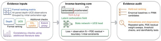
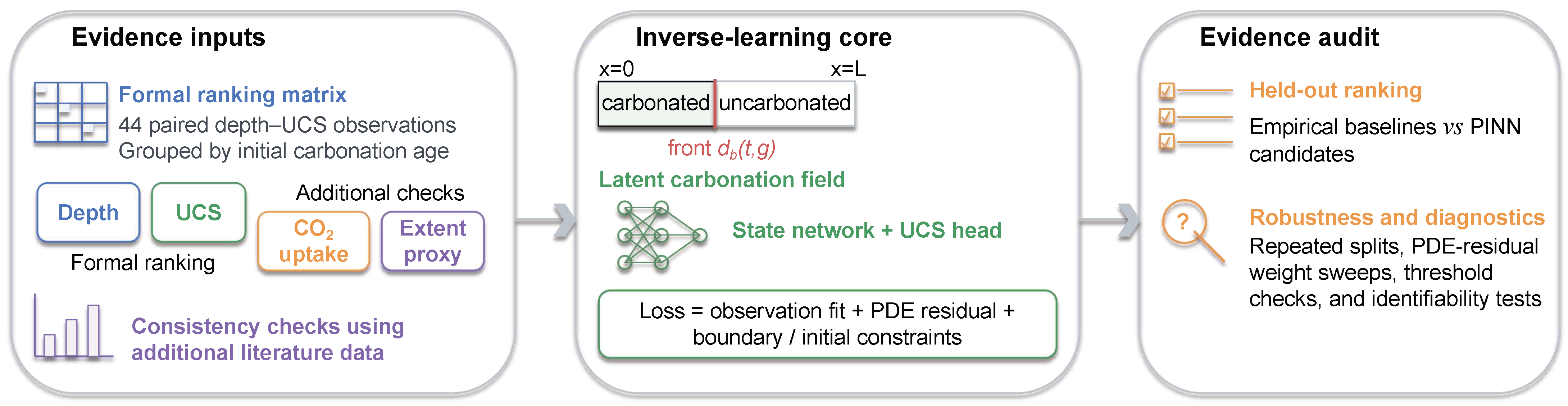
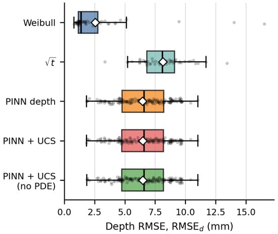
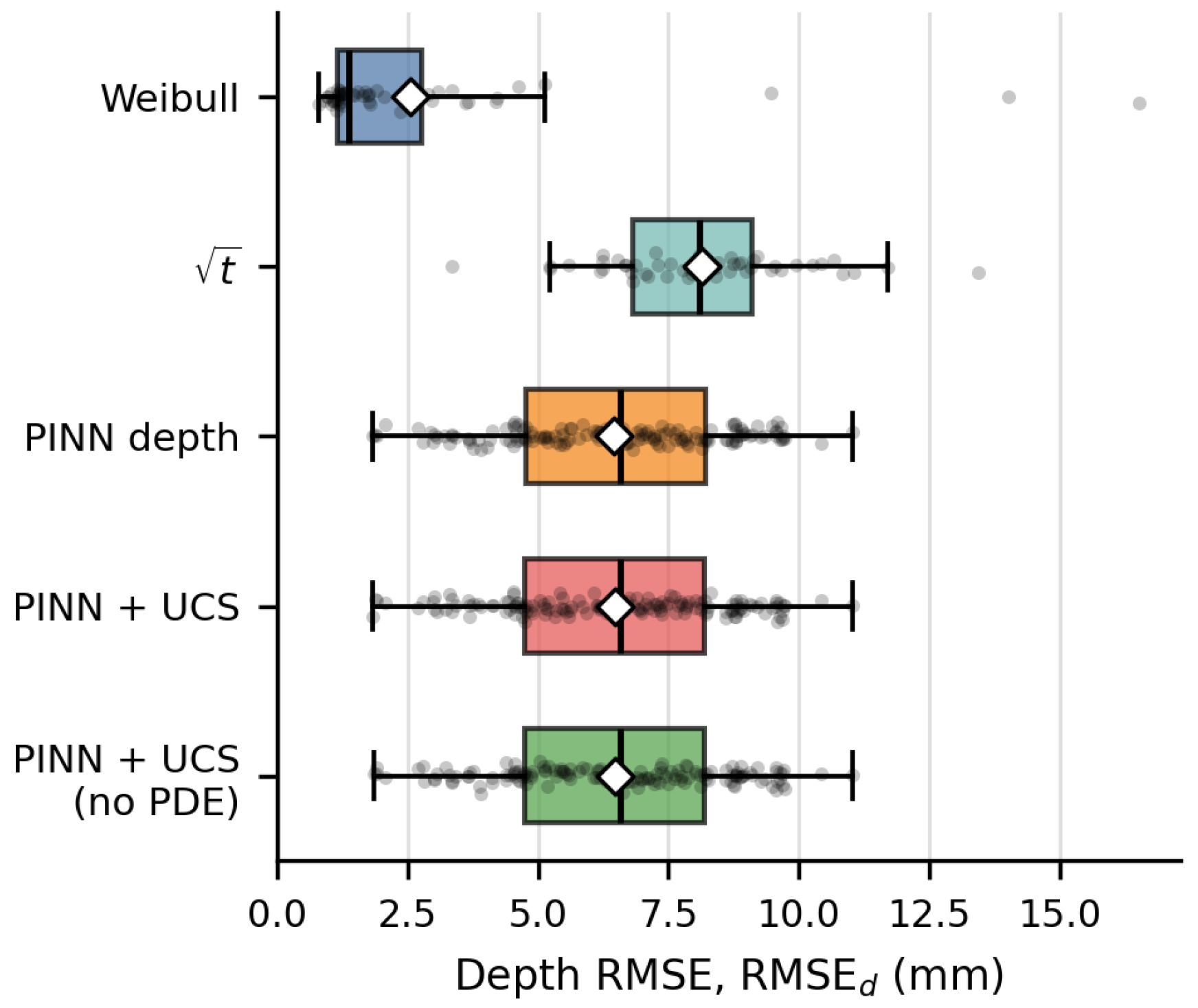
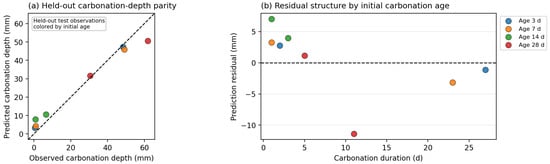
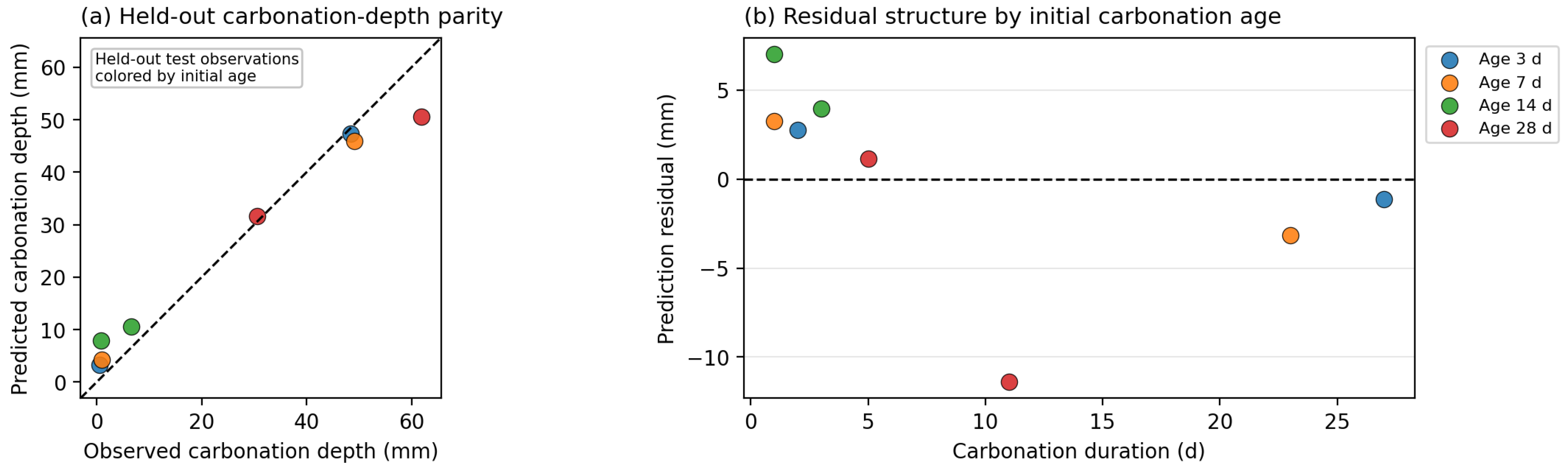
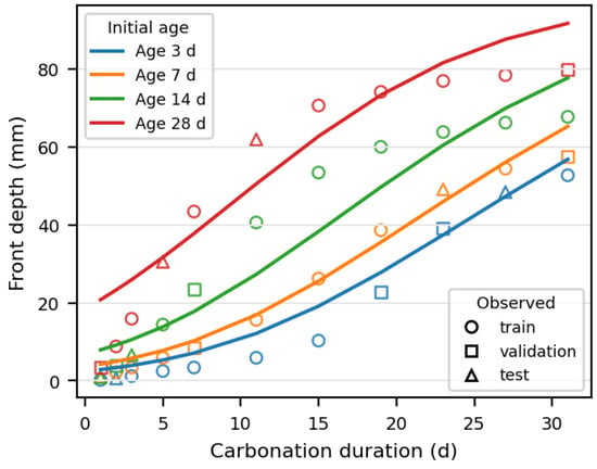
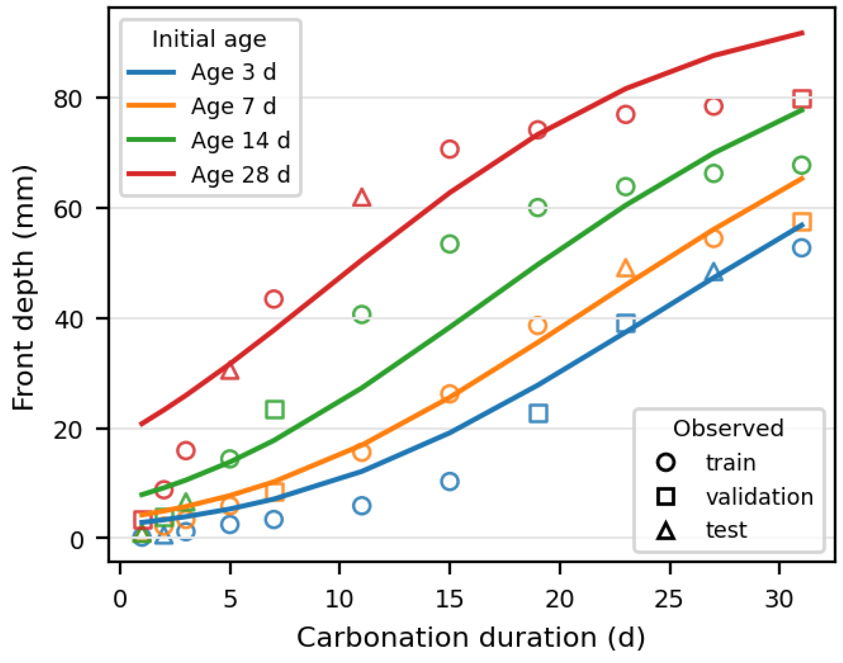
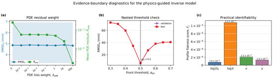
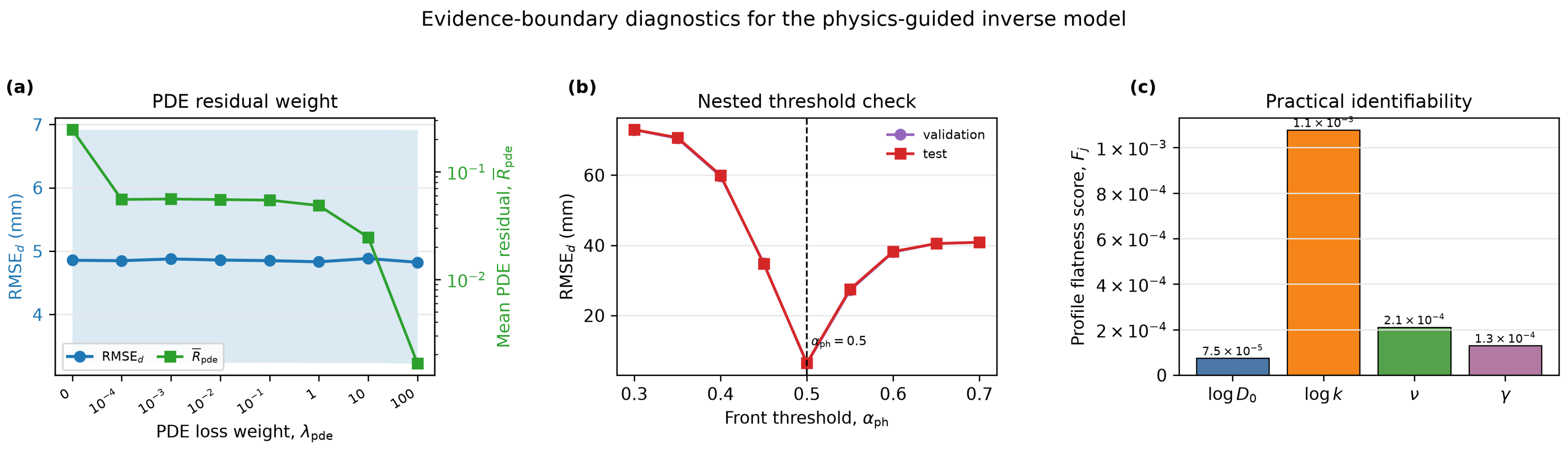
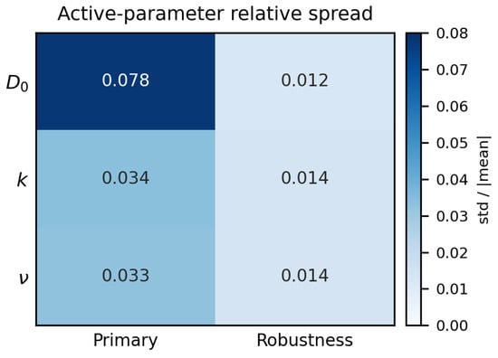
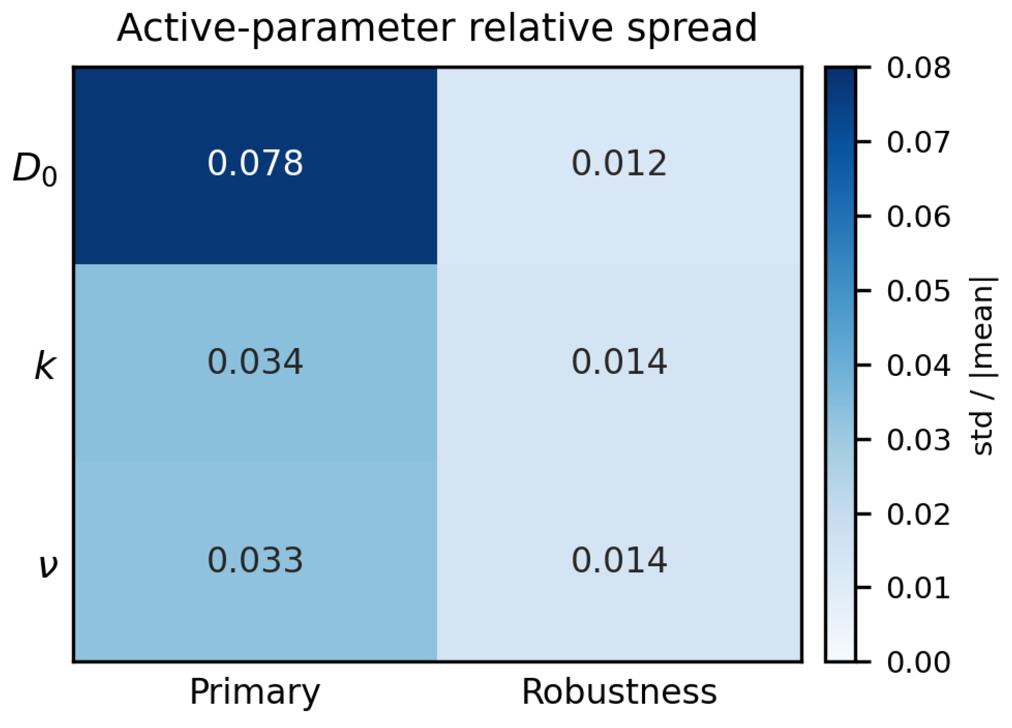
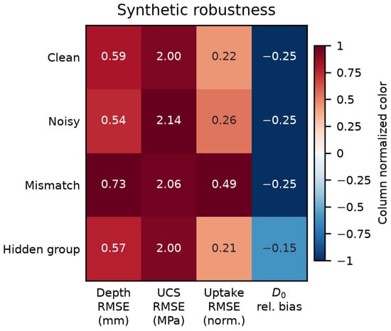
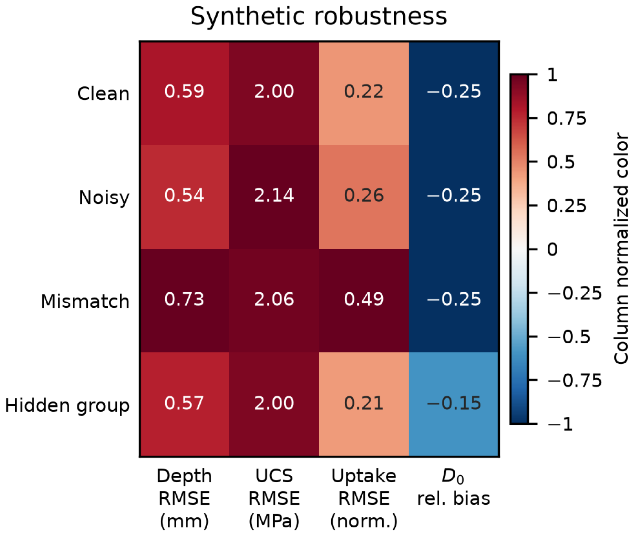
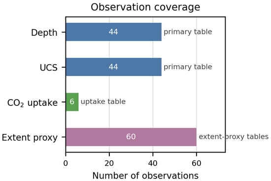
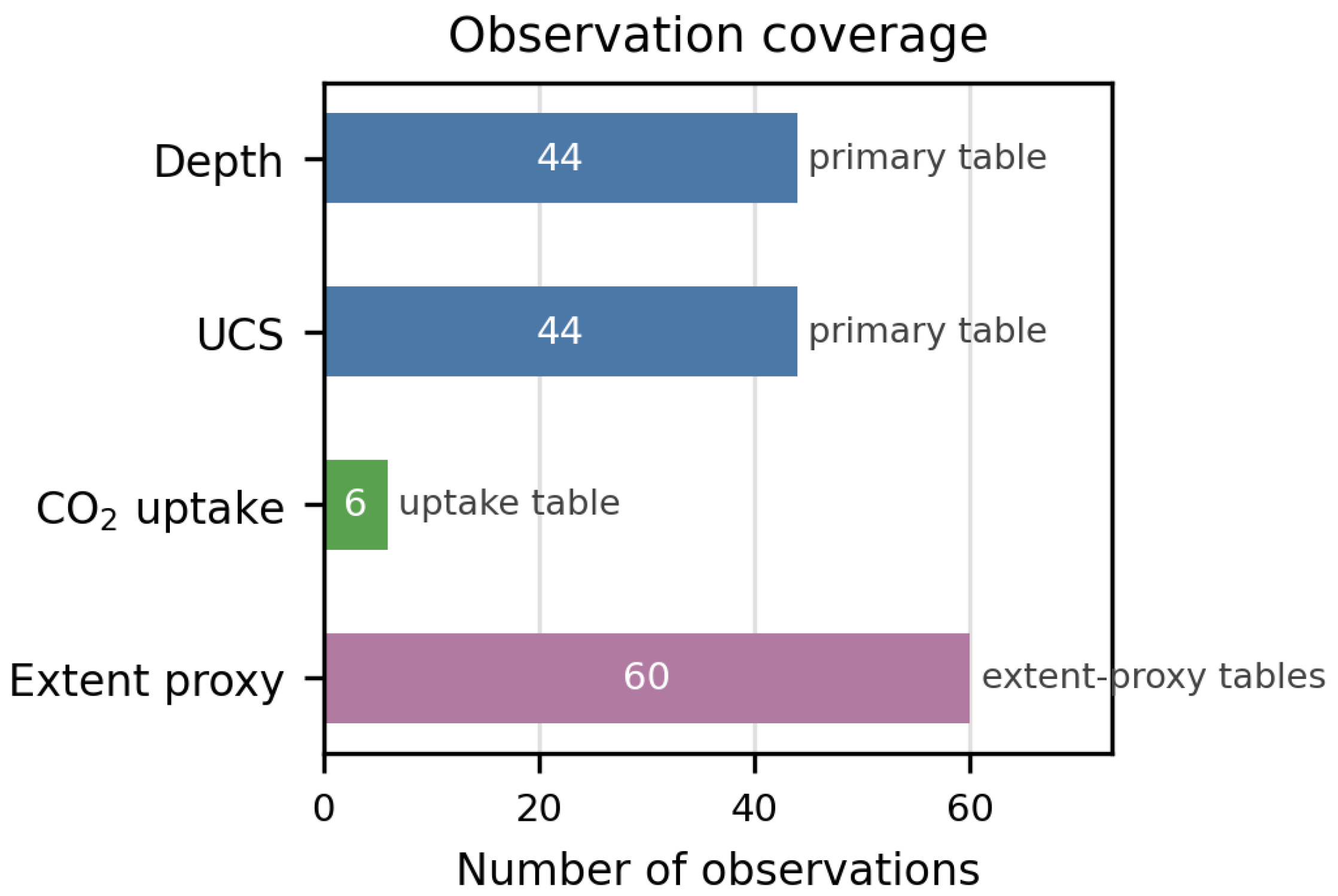
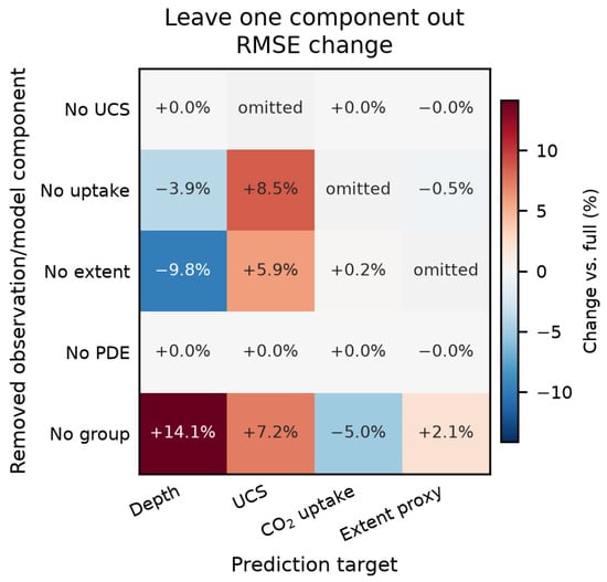
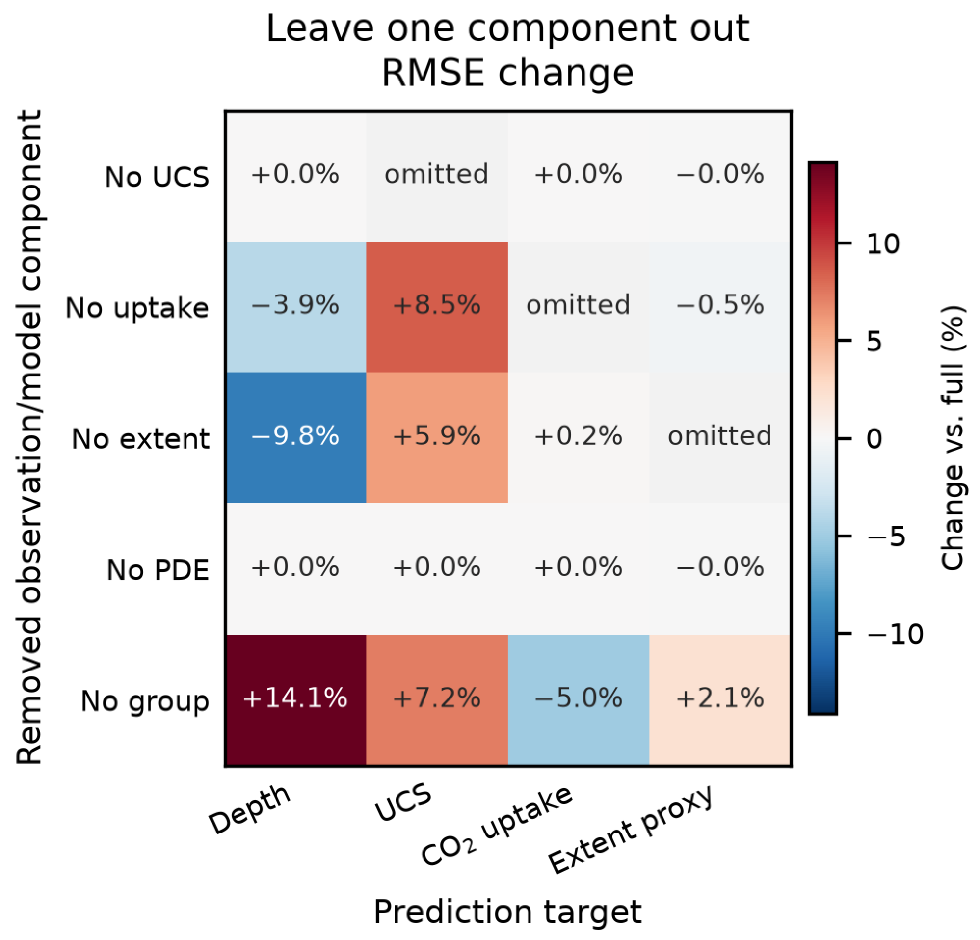

Disclaimer/Publisher’s Note: The statements, opinions and data contained in all publications are solely those of the individual author(s) and contributor(s) and not of MDPI and/or the editor(s). MDPI and/or the editor(s) disclaim responsibility for any injury to people or property resulting from any ideas, methods, instructions or products referred to in the content. |
© 2026 by the authors. Licensee MDPI, Basel, Switzerland. This article is an open access article distributed under the terms and conditions of the Creative Commons Attribution (CC BY) license.