


Abstract
Autism spectrum disorder (ASD) is a heterogeneous neurodevelopmental condition, and objective identification based on neuroimaging remains challenging due to inter-subject variability, multi-site heterogeneity, and the complex topology of brain functional networks. Resting-state functional magnetic resonance imaging (rs-fMRI) provides a non-invasive way to characterize intrinsic brain activity, but existing functional-connectivity-based methods often rely on single-scale static representations and insufficiently capture high-order topology, temporal evolution, and phenotypic heterogeneity. This study aims to develop a mathematical and AI-based brain-network modeling framework for ASD identification from rs-fMRI. The proposed method integrates low-order functional connectivity, high-order functional connectivity, phenotypic information, dynamic graph sequences, Transformer-based temporal attention, and static–dynamic gated fusion. Experiments were conducted on the ABIDE-I dataset, including 1112 subjects from 17 acquisition sites, with 539 ASD subjects and 573 typical controls. The proposed static multi-channel model achieved an accuracy of 75.8%, while the dynamic extension achieved a mean accuracy of 78.5% ± 0.7% and an AUC of 0.84 ± 0.01 over repeated runs. The results suggest that jointly modeling multi-scale static topology and dynamic temporal evolution may improve rs-fMRI-based ASD identification and offer a computationally interpretable framework for AI-assisted neuroimaging analysis.
Keywords:
autism spectrum disorder; resting-state functional magnetic resonance imaging; graph neural networks; multi-channel fusion; temporal attention; dynamic brain networks MSC:
68T07; 68T09
1. Introduction
Autism spectrum disorder (ASD) is a highly heterogeneous neurodevelopmental disorder characterized by persistent impairments in social communication and social interaction, together with restricted interests and repetitive behaviors. Because ASD symptoms often emerge early in development but vary substantially across individuals, early identification is important for intervention planning and long-term support. In current clinical practice, ASD diagnosis still relies primarily on behavioral observation and standardized assessments, which may be influenced by symptom heterogeneity, developmental stage, evaluator experience, and individual differences. Therefore, objective neuroimaging-based auxiliary analysis has become an important direction for understanding the neural basis of ASD and developing data-driven tools for AI-assisted neuroimaging analysis. Among available modalities, resting-state functional magnetic resonance imaging (rs-fMRI) is particularly attractive because it can noninvasively characterize spontaneous brain activity and resting-state functional organization without requiring subjects to perform explicit tasks [1,2,3]. Brain network analysis based on rs-fMRI further provides a computational pathway for studying links between atypical functional organization and individualized ASD identification.
From a mathematical perspective, rs-fMRI data can be represented at multiple levels, including high-dimensional temporal signals, functional-connectivity matrices, and graph-structured brain networks. After parcellating the brain into regions of interest, the regional blood-oxygen-level-dependent time series form a temporal signal matrix, while statistical dependencies between pairs of regional signals define a whole-brain functional-connectivity matrix. In graph-based formulations, brain regions are treated as nodes, functional connections are encoded as weighted edges, and the connectivity matrix serves as the adjacency structure of the brain graph. This representation makes it possible to analyze ASD-related differences from the perspectives of signal interactions, network topology, and graph-based representation learning [4,5,6,7]. Existing studies have shown that ASD is associated with abnormalities in long-range functional coupling, inter-network coordination, hemispheric synchronization, and temporal switching among latent brain states [1,8,9,10]. These abnormalities do not appear only in isolated regions; rather, they are embedded in the topology and dynamics of whole-brain functional networks, which motivates mathematical and AI-based brain network modeling for ASD identification.
Despite this progress, several methodological limitations remain unresolved. First, many existing studies still rely mainly on low-order static functional connectivity derived from pairwise correlations over the whole scan. Although this representation captures direct statistical coupling between pairs of regions, it may be insufficient for describing the hierarchical and multi-scale organization of complex brain networks [4,11,12]. Second, high-order topological similarity is often not adequately modeled. Shared neighborhood structure, similarity between connectivity profiles, and indirect interaction patterns are frequently ignored or treated only as auxiliary descriptors, rather than being integrated as explicit graph representations. Third, dynamic functional connectivity and temporal dependencies remain underutilized. Static graph models compress the full rs-fMRI sequence into a single connectivity matrix and may therefore average out transient network states, temporal switching patterns, and time-varying ASD-related abnormalities [9,10,13,14,15]. Finally, phenotypic information and site heterogeneity are still insufficiently handled. Variables such as age, sex, and acquisition site contain important complementary information, but they are often appended in a shallow manner and are not fully fused with imaging-derived graph representations [4,16].
To address these limitations, this study proposes a mathematical and AI-based brain-network modeling framework that jointly models multi-scale functional connectivity, temporal dynamics, and phenotypic information. Specifically, low-order functional connectivity (LOFC) is used to describe direct regional coupling, high-order functional connectivity (HOFC) is constructed to characterize topological similarity among connectivity profiles, and sliding-window dynamic graph sequences are introduced to represent temporal evolution in brain functional organization. On this basis, the framework combines multi-channel graph learning, Transformer-based temporal attention, and static–dynamic gated fusion to learn discriminative representations for individualized ASD identification. Phenotypic information is further introduced as an auxiliary channel to support multimodal integration under inter-subject and multi-site heterogeneity [16,17,18].
The main contributions of this paper are summarized as follows:
- 1.
- Mathematical representation of rs-fMRI brain networks. We formulate rs-fMRI-based ASD identification as a biomedical graph representation learning problem and construct low-order and high-order functional connectivity matrices to describe direct functional coupling and higher-order topological similarity.
- 2.
- AI-based multi-channel brain-network learning. We design a multi-channel graph neural network to jointly model low-order connectivity, high-order connectivity, and phenotypic information, enabling complementary integration of imaging-derived and subject-level biomedical features.
- 3.
- Static–dynamic functional connectivity fusion. We introduce dynamic graph sequences based on sliding windows and combine shared-parameter GCNs with Transformer-based temporal attention to model temporal evolution in brain functional organization.
- 4.
- Interpretable and reproducible biomedical informatics evaluation. We validate the framework on the public ABIDE-I dataset and conduct comparison, ablation, parameter sensitivity, robustness, and interpretability analyses to evaluate its potential for AI-assisted ASD identification.
The remainder of this paper is organized as follows. Section 2 reviews related work from four perspectives: resting-state functional connectivity studies in ASD, graph neural networks for brain network modeling, dynamic temporal modeling, and foundation-model or prompt-based AI methods in neuroimaging. Section 3 presents the proposed method, including multi-scale static connectivity construction, multi-channel graph modeling, and dynamic temporal extension. Section 4 describes the experimental design and reports comparative, ablation, and parameter-analysis results. Section 5 discusses the observed strengths and limitations of the proposed framework under the current setting. Finally, Section 6 concludes the paper and outlines future research directions.
2. Related Work
The literature on ASD identification with rs-fMRI can be broadly organized into four closely related directions: resting-state functional connectivity analysis, graph representation learning on functional brain networks, dynamic spatiotemporal modeling, and recent foundation-model or prompt-based AI methods in neuroimaging. Although these directions share the goal of extracting discriminative features from whole-brain activity, they differ in their modeling assumptions, representational granularity, and treatment of temporal or multimodal information. Taken together, they suggest that ASD-related abnormalities are multi-faceted and cannot be fully explained by any single type of connectivity descriptor.
A common trend across recent studies is the gradual shift from descriptive neuroimaging analysis to end-to-end computational models. Early work mainly focused on identifying group differences in specific networks or graph metrics, whereas later studies increasingly emphasized machine-learning-based subject-level prediction. More recent methods further incorporate graph neural networks, self-attention, multimodal fusion, and foundation-model ideas to improve generalization and interpretability. Nevertheless, existing approaches are still often specialized to a single representation regime, such as static pairwise connectivity, dynamic window-based connectivity, image-level representation learning, or text-oriented prompt reasoning, which motivates more unified frameworks for ROI-level rs-fMRI brain networks.
2.1. rs-fMRI Functional Connectivity and ASD Brain Network Analysis
Resting-state fMRI has become one of the most important neuroimaging tools for ASD research because it can characterize intrinsic brain functional organization without requiring task execution. Functional connectivity analysis has shown that ASD is associated with atypical coordination among distributed brain systems, including reduced interhemispheric synchronization, abnormal long-range coupling, and disrupted integration across large-scale functional networks [1,8]. These findings support the view that ASD-related neural alterations are not restricted to isolated regions, but are reflected in network-level patterns of functional interaction.
In this context, rs-fMRI brain network analysis provides a bridge between neuroimaging feature extraction and computational identification. Brain regions can be represented as nodes, functional dependencies between regional time series can be encoded as edges, and the resulting connectivity matrix can be analyzed as a whole-brain graph. Static functional connectivity summarizes the full scan into a single network and is useful for capturing stable coupling patterns, whereas dynamic functional connectivity uses time-resolved representations to describe temporal fluctuations and state transitions in brain organization [9,10,13]. Together, these two perspectives indicate that both stable network topology and time-varying connectivity may contribute to ASD identification.
The release of the Autism Brain Imaging Data Exchange datasets substantially advanced this field by providing larger multi-site rs-fMRI samples for algorithm development and reproducible evaluation [2,3]. ABIDE has enabled researchers to examine ASD-related abnormalities across default-mode, salience, sensory, attention, and other functional systems, and to evaluate models under more realistic inter-subject variability [19,20]. At the same time, the multi-site nature of ABIDE introduces heterogeneity caused by differences in scanners, acquisition protocols, preprocessing pipelines, age distributions, and phenotypic composition. Therefore, ASD brain network analysis may benefit from models that extract discriminative connectivity patterns while accounting for site variability and subject-level heterogeneity.
2.2. Graph Neural Networks for Brain Network Modeling
A second major direction focuses on graph neural networks for brain network modeling. Since functional connectivity naturally forms a non-Euclidean graph structure, graph-based methods are well suited to preserving topological relationships among brain regions. Early computational approaches often relied on handcrafted graph metrics or vectorized connectivity features, whereas graph convolutional networks (GCNs) directly propagate information over adjacency structures and learn node- or graph-level representations from functional brain networks [4,11,12]. These models have been widely applied to graph-based ASD classification because they can combine connectivity topology with discriminative feature learning.
Several graph learning paradigms have been explored for ASD identification. Population graph methods construct subject-level graphs in which nodes correspond to individuals and edges encode phenotypic or imaging-based similarity, allowing label-related information to propagate across demographically related subjects [4]. Brain-graph GCN models instead treat each subject’s functional connectivity matrix as a graph and learn representations from regional interactions [12]. Graph attention networks (GATs) further introduce attention weights to adaptively emphasize informative brain regions or functional connections, improving interpretability and flexibility in functional brain network classification [5,6,7]. These studies suggest that graph-based ASD classification may benefit from explicitly modeling both network topology and discriminative regional interactions.
More recent studies have extended graph neural networks with attention mechanisms, multimodal fusion, and transformer-style architectures. Attention graph convolution has been used to improve adaptation and feature selection in brain disorder identification [11], while residual graph transformers and related architectures aim to capture long-range dependencies within functional connectivity graphs [21]. Other studies have incorporated structural–functional fusion or nonlinear representation interpretation to support representation stability and biological interpretability [16,17,22]. Nevertheless, many graph-based ASD classifiers still emphasize static or single-view connectivity, and they do not fully integrate low-order connectivity, high-order topological similarity, temporal dynamics, and phenotypic information in a unified framework.
2.3. Dynamic Functional Connectivity and Temporal Attention
The third direction emphasizes dynamic functional connectivity and temporal attention. Instead of assuming that a single static connectivity matrix can fully summarize the entire scan, dynamic approaches usually divide rs-fMRI time series into overlapping sliding windows and compute a sequence of window-specific functional connectivity graphs. This sliding-window strategy allows the model to characterize transient connectivity states, temporal variability, and state-transition patterns that may be averaged out by static functional connectivity [9,10,13]. Such temporal information is especially relevant for ASD because atypical brain organization may involve instability in functional coordination rather than only persistent differences in mean connectivity strength.
Sequence models have therefore been introduced to learn temporal dependencies from dynamic connectivity representations. Recurrent architectures such as long short-term memory (LSTM) and gated recurrent unit (GRU) networks can model ordered connectivity sequences and capture dependencies across consecutive windows. More recently, Transformer-based models and temporal attention mechanisms have been used to assign adaptive importance to different time windows, identify informative temporal states, and model long-range dependencies more effectively than purely recurrent structures. Representative studies include hidden-Markov and dynamic-graph analyses of spatiotemporal brain activity [14], self-attention extraction on aligned dynamic connectivity [15], multi-task transformer models [23], dynamic graph transformer networks [18], and probabilistic spatiotemporal graph learning frameworks [24].
Despite these advances, dynamic models still face challenges related to window-length sensitivity, computational cost, and integration with static global topology. Many methods focus either on static graph classification or on dynamic sequence modeling, treating the two representations as separate paradigms rather than complementary sources of information. Static–dynamic fusion is therefore an important direction for ASD identification: static graphs can encode stable whole-brain topology, while dynamic graph sequences can capture temporal evolution and transient network states. Recent graph-learning and transformer-based ASD studies further suggest the value of combining multi-view connectivity, temporal attention, and adaptive fusion mechanisms [25,26,27,28,29]. This motivates the present framework, which jointly models multi-scale static connectivity, dynamic temporal evolution, and phenotypic information through static–dynamic gated fusion.
2.4. Foundation Models, Large Vision Models and Prompt-Based AI in Neuroimaging
Recent advances in foundation models, large vision models, and prompt-based large language models (LLMs) have opened new opportunities for medical image analysis and text-based reasoning. Large vision or vision–language models can learn transferable representations from large-scale medical images, while prompt-based LLMs can support report generation, question answering, semantic reasoning, and multimodal explanation [30,31]. In neuroimaging, related efforts have begun to explore foundation-style models for brain connectivity and connectome representation learning, including graph-transformer-based pretraining on large functional connectivity networks [32].
However, the direct application of large vision models to ROI-level rs-fMRI connectivity graphs is not straightforward. The input of the present study is not a natural image, a raw MRI slice, or a voxel-level volume, but a set of graph-structured functional-connectivity representations derived from regional BOLD time series. Such data are characterized by non-Euclidean topology, symmetric connectivity matrices, dynamic graph sequences, and subject-level phenotypic variables. Similarly, prompt-based LLMs are more naturally suited to clinical reports, textual reasoning, literature-level interpretation, or multimodal explanation than to direct graph classification from rs-fMRI connectivity matrices. Therefore, this study focuses on graph-based and temporal modeling methods that are directly comparable under the ROI-level rs-fMRI setting, while recent foundation-model-based neuroimaging and prompt-based AI methods are discussed as future directions for scalable pretraining, cross-dataset transfer, and explainable neuroimaging analysis.
As summarized in Table 1, existing studies usually emphasize either static graph topology, dynamic temporal modeling, or multimodal fusion. In contrast, the proposed framework jointly integrates low-order connectivity, high-order topological similarity, phenotypic information, dynamic graph sequence learning, and static–dynamic gated fusion under a unified rs-fMRI brain-network modeling pipeline.
Table 1.
State-of-the-art comparison of representative AI methods for rs-fMRI brain-network and neuroimaging analysis.
3. Method
3.1. Problem Formulation
For each subject, the input is the rs-fMRI ROI time-series matrix denoted as , where N represents the number of brain regions of interest and T denotes the number of temporal frames. The output is a binary ASD identification label , where ASD and typical control (TC) subjects are encoded as two classes. In addition to imaging data, each subject is associated with a phenotypic vector , including age, sex, acquisition site, and other available subject-level variables.
The objective of rs-fMRI-based ASD identification is to learn a prediction function
which maps the ROI time series and phenotypic variables to the ASD/TC classification label. To make the rs-fMRI signal suitable for graph representation learning, is first transformed into multiple brain-network representations, including the low-order functional connectivity (LOFC) matrix, the high-order functional connectivity (HOFC) matrix, and a dynamic graph sequence generated from sliding temporal windows. These representations jointly describe direct functional coupling, higher-order topological similarity, and temporal evolution of brain functional organization, respectively.
3.2. Overall Framework
The proposed method consists of two components: static multi-channel graph modeling and a dynamic temporal extension (Figure 1) and the learning workflow is summarized in Algorithm 1. The static component constructs LOFC and HOFC brain networks from the full rs-fMRI time series and integrates phenotypic information into a multi-channel GCN architecture. The dynamic component builds LOFC/HOFC graph sequences using sliding time windows, applies shared-parameter GCNs to extract graph features from each temporal slice, captures long-range temporal dependencies with a Transformer, and finally performs gated fusion with the static branch.
| Algorithm 1 Multi-Scale Static–Dynamic Brain Network Learning Framework |
|
Figure 1.
Overall framework of the proposed mathematical and AI-based brain-network modeling method.
3.3. Construction of Multi-Scale Static Functional Connectivity
3.3.1. Low-Order Functional Connectivity
For each subject, let the brain-region time-series matrix extracted based on the AAL atlas be , where is the number of regions of interest and T is the number of time points. The LOFC matrix is computed using the Pearson correlation coefficient
Because Pearson correlation coefficients are bounded in and may have non-constant variance, a Fisher-z transformation is applied before subsequent graph construction
where correlation values are clipped slightly away from for numerical stability, and the diagonal elements are set to zero. The Fisher-z transformed matrix is used as the weighted LOFC representation in the following graph construction steps.
To suppress noisy connections and construct a sparse brain graph, a proportional thresholding strategy is used to preserve the top 20% absolute connections
where is the subject-specific percentile threshold. The proportional threshold was applied within each subject to preserve the strongest 20% absolute connections. The threshold ratio was selected based on validation performance and kept fixed for all subjects and all methods requiring sparse graphs.
LOFC captures pairwise signal-level dependency, whereas HOFC captures similarity between connectivity profiles and therefore reflects higher-order network organization.
3.3.2. High-Order Functional Connectivity
High-order functional connectivity is used to characterize the topological similarity of brain regions within the whole-brain network. This paper first constructs topological high-order functional connectivity, denoted as tHOFC. Specifically, after the LOFC matrix is obtained, the i-th row of the Fisher-z transformed LOFC matrix is regarded as the connectivity-profile fingerprint of brain region i, denoted by . The HOFC edge between regions i and j is then defined as the Pearson correlation between their connectivity profiles
In this way, two brain regions are considered highly connected in the HOFC graph if they show similar whole-brain connectivity patterns, even when their direct pairwise LOFC value is not strong. This representation complements LOFC by encoding indirect and higher-order topological similarity.
Furthermore, to obtain a more data-adaptive high-order representation, adaptive high-order functional connectivity (aHOFC) is introduced. The computational procedure consists of five steps. First, the LOFC matrix is computed for each subject as described above. Second, each row of the LOFC matrix is treated as a connectivity-profile vector. Third, ROI profiles are clustered into K groups, resulting in a clustering indicator matrix . Fourth, the adaptive high-order matrix is estimated by minimizing the sparse reconstruction objective
where is the sparsity regularization coefficient. Finally, the adaptive high-order adjacency matrix is obtained as
and it is symmetrized, normalized, and used as the HOFC adjacency matrix in the graph learning branch.
The objective is solved using alternating optimization. With fixed, is updated by sparse least-squares optimization with regularization. With fixed, is updated based on clustering of connectivity-profile vectors. The optimization stops when the relative objective change is below or when the maximum number of iterations reaches 100. The candidate values and selected settings for HOFC construction are summarized in Table 2.
Table 2.
Parameter selection for HOFC construction and sparse graph generation.
All HOFC-related parameters were selected using only training and validation data. Test-set information was not used during parameter selection, and the selected values were then fixed for test-set evaluation and for all baseline methods requiring sparse graph construction.
3.4. Static Multi-Channel GCN Modeling
3.4.1. Node Features and Phenotype Encoding
In addition to adjacency matrices, graph convolutional networks also require node features. For each brain region, the following features are constructed: node degree, clustering coefficient, betweenness centrality, nodal efficiency, MNI spatial coordinates, local activity measures (such as ALFF and ReHo), and functional system affiliation encoding. Z-score normalization is applied to each feature dimension
For phenotypic variables such as sex, age, and acquisition site, one-hot encoding or numerical standardization is first applied, and the resulting features are then fed into an MLP to obtain a phenotypic embedding vector . This phenotype representation can either participate in fusion as an independent channel or be injected into node features through a linear projection.
3.4.2. Multi-Channel GCN Branches
Both the LOFC and HOFC channels adopt a three-layer GCN architecture, with hidden dimensions set to . A single graph convolution layer is defined as
where , is the degree matrix, and denotes the learnable parameters of the l-th layer. Each layer is followed by batch normalization, LeakyReLU, and Dropout. The graph-level representation is obtained by global average pooling
The phenotype channel uses a three-layer MLP to extract a vector representation and modulates graph features in a gated manner
where ⊙ denotes element-wise multiplication.
3.4.3. Channel Fusion and Classification
Three fusion strategies are considered in this study: simple concatenation, weighted summation, and attention-based fusion. The best-performing strategy is attention fusion, formulated as
where denotes the graph-level features of different channels. The classification head consists of a two-layer fully connected network with a sigmoid output.
3.5. Dynamic Graph Sequence Construction and Temporal Modeling
3.5.1. Dynamic Graph Sequence Generation
To explicitly model the temporal evolution of brain functional connectivity, a sliding-window strategy was used to construct dynamic graph sequences from the preprocessed rs-fMRI ROI time series. Let the window length be L, the step size be S, and the total number of time points be T. The number of temporal windows for each subject is calculated as
In this study, the window length was set to TR and the step size was set to TR. The choice of a 50-TR window was made to balance the statistical stability of functional-connectivity estimation and the sensitivity to transient connectivity fluctuations. A shorter window may contain insufficient temporal samples for reliable Pearson correlation estimation, resulting in unstable dynamic connectivity matrices. In contrast, an overly long window may smooth out short-term variations in brain-network states and weaken the model’s ability to capture transient ASD-related functional patterns. Therefore, the 50-TR setting was selected as a compromise between estimation reliability and temporal sensitivity.
The step size of 5 TR corresponds to a high overlap ratio between adjacent windows. This setting was adopted to preserve temporal continuity in the dynamic graph sequence and to reduce abrupt changes between neighboring connectivity matrices. Although highly overlapping windows may introduce redundancy, all dynamic windows generated from the same subject were assigned to the same data partition during training, validation, and testing. Therefore, window-level leakage across different partitions was avoided, and classification was performed at the subject level rather than at the individual-window level.
For each temporal window, both low-order functional connectivity and high-order functional connectivity were computed. Specifically, the LOFC matrix was calculated using Pearson correlation between regional time series within the current window, and the HOFC matrix was computed based on the similarity between window-specific connectivity profiles. The top 20% of connections ranked by absolute value were retained to construct sparse dynamic adjacency matrices. This procedure generated a two-channel dynamic graph sequence consisting of time-resolved LOFC and HOFC graphs.
Because scan durations vary across ABIDE-I acquisition sites, different subjects may produce different numbers of dynamic windows. To enable batch training and temporal attention modeling, all dynamic graph sequences were aligned to a fixed sequence length. For sequences longer than the target length, uniform temporal sampling or truncation was applied. For sequences shorter than the target length, linear interpolation was used to obtain a sequence with the required length. This sequence alignment was performed at the dynamic graph representation level rather than on the raw BOLD signals, so as to avoid modifying the original rs-fMRI time series.
To ensure numerical validity, each window-specific connectivity matrix was checked after construction. Invalid windows were defined as windows that produced non-finite connectivity values, such as NaN or Inf entries, after correlation computation. Since quality-controlled preprocessed ROI-level time series were used, such cases were rare. No invalid windows were observed after preprocessing and connectivity construction in the final cohort. No additional window-level exclusion was performed unless a subject failed to produce a valid dynamic graph sequence.
The resulting aligned dynamic graph sequence for each subject can be represented as
where denotes the fixed sequence length after alignment. This dynamic graph representation allows the subsequent shared-parameter GCN and temporal attention modules to jointly learn window-level spatial features and long-range temporal dependencies of brain functional networks.
3.5.2. Shared-Parameter GCN
For the w-th time window, shared-parameter GCNs are applied to the LOFC graph and HOFC graph, respectively, to extract graph-level representations
The shared-parameter mechanism ensures that representations from different temporal slices lie in a unified feature space and significantly reduces the parameter scale. The two channels are then concatenated along the feature dimension to form a temporal feature matrix
The shared-parameter design ensures that all temporal windows are encoded in the same feature space. This is important for temporal attention because the Transformer encoder assumes that the input sequence elements are comparable across time. In addition, parameter sharing reduces model complexity and helps prevent overfitting under limited neuroimaging sample sizes. The prediction remains subject-level rather than window-level. All window-level embeddings generated from one subject are aggregated into a single dynamic representation before classification.
3.5.3. Temporal Attention Mechanism
To learn long-range temporal dependencies, a Transformer encoder is employed to model the temporal feature matrix. The core self-attention computation is
where
Multi-head attention together with a feed-forward network, residual connections, and layer normalization forms the Transformer Encoder. After temporal modeling, the output vector of the dynamic branch, , is obtained by global average pooling.
Compared with global average pooling, temporal attention preserves the order and relative importance of dynamic brain states. Compared with recurrent models such as LSTM, the Transformer encoder can model long-range dependencies between non-adjacent windows more directly and is less affected by gradient attenuation in long dynamic sequences.
3.5.4. Static–Dynamic Dual-Branch Fusion
The output of the static branch, , is obtained from the static multi-channel GCN built on the full scan. The output of the dynamic branch, , comes from the Transformer-encoded dynamic graph sequence. The two are fused through gating
To improve consistency between the two branches, the training loss is defined as
where is the binary cross-entropy loss and is the consistency constraint between the predictions of the static and dynamic branches. More specifically,
where denotes the final fused ASD probability, and and denote the branch-level predictions from the static and dynamic branches, respectively. The gate in the fusion module is subject-adaptive because it is computed from the static and dynamic representations of each individual sample, allowing the model to reduce the contribution of a noisy dynamic branch when temporal-window estimates are unstable.
3.5.5. Computational Complexity Analysis
To further evaluate the computational feasibility of the proposed framework, we analyze the approximate computational complexity of the main modules and compare it with representative baseline models. Let N denote the number of brain regions of interest, T the number of rs-fMRI time points, W the number of dynamic temporal windows, E the number of retained graph edges after sparse thresholding, d the hidden feature dimension, the number of graph convolutional layers, and H the number of attention heads. In this study, the AAL atlas was used, and therefore .
First, the construction of the low-order functional connectivity (LOFC) matrix requires computing pairwise Pearson correlations between all pairs of brain regions. The corresponding computational complexity is approximately
For high-order functional connectivity (HOFC), each row of the LOFC matrix is treated as a connectivity-profile vector, and the similarity between connectivity profiles of different brain regions is further computed. Since each profile has dimension N, the approximate complexity of HOFC construction is
Although this step is more expensive than LOFC construction, the computational cost remains manageable because the analysis is performed at the ROI level rather than at the voxel level.
For graph representation learning, the complexity of one graph convolutional layer on a sparse graph is approximately
where E is the number of retained edges and d is the hidden feature dimension. For an -layer GCN, the complexity becomes
In the static branch, graph convolution is performed on the LOFC and HOFC graphs derived from the full rs-fMRI sequence. Therefore, the main computational cost of the static branch is approximately
where denotes the number of static graph channels. In this study, for the LOFC and HOFC channels, while the phenotypic-information branch is implemented by a lightweight multilayer perceptron and has much lower computational cost compared with graph convolution.
In the dynamic branch, LOFC and HOFC graphs are constructed for each temporal window. The shared-parameter GCN is then applied to each window-level graph. Since the same GCN parameters are reused across all windows, the number of trainable parameters does not increase with W, although the forward computation scales linearly with the number of windows. The approximate complexity of the dynamic graph convolution module is therefore
where denotes the two dynamic graph channels, namely dynamic LOFC and dynamic HOFC.
After obtaining window-level graph representations, a Transformer-based temporal attention module is applied to model long-range dependencies across dynamic brain states. Since temporal attention is performed on the sequence of window-level embeddings rather than on raw voxel-level signals, its complexity is
where W is the number of temporal windows after sequence alignment. Because W is much smaller than the number of voxels or raw time-series samples, this temporal attention module remains computationally feasible in the present ROI-level setting.
Combining the above components, the overall computational complexity of the proposed framework can be approximated as
Since and are small constants in this study, the expression can be simplified as
This indicates that the main additional computational costs of the proposed model come from HOFC construction, dynamic graph sequence modeling, and temporal attention. However, sparse graph construction, ROI-level representation, and shared-parameter GCNs help control the overall computational burden.
For comparison, Table 3 summarizes the approximate computational complexity of the proposed method and representative baseline approaches. Compared with a single static GCN, the proposed model introduces additional costs through HOFC construction and dynamic temporal modeling. Compared with more complex Transformer-based baselines, however, the proposed method applies temporal attention to compact graph-level window embeddings rather than to high-dimensional raw neuroimaging signals, which helps maintain a reasonable balance between representation capacity and computational efficiency.
Table 3.
Approximate computational complexity of the proposed method and representative baseline models.
Overall, the proposed framework is computationally more expensive than a single static GCN, but the additional cost is mainly associated with modeling high-order topology and dynamic temporal dependencies. These components are central to the proposed method because they allow the model to characterize both stable functional-network organization and time-varying connectivity patterns. In practice, the use of the AAL-116 atlas, proportional sparse thresholding, shared-parameter GCNs, and temporal attention over window-level embeddings makes the method computationally feasible for ABIDE-I scale rs-fMRI analysis.
4. Experimental Design
4.1. Dataset and Sample Selection
The experiments in this study were conducted on ABIDE-I from the Autism Brain Imaging Data Exchange (ABIDE), a large-scale public neuroimaging resource initiated by the international brain-imaging research community for autism spectrum disorder (ASD) research. The goal of the ABIDE consortium is to integrate data collected by multiple research institutions worldwide and to establish a large-sample, multi-site neuroimaging database for ASD. As an open data-sharing initiative, ABIDE has substantially promoted the development and validation of data-driven methods for ASD identification.
ABIDE-I was released in 2012 and contains data from 1112 participants collected at 17 international acquisition sites, including 539 individuals with ASD and 573 typical controls (TC). The included sites are CALTECH, CMU, KKI, LEUVEN, MAX_MUN, NYU, OHSU, OLIN, PITT, SBL, SDSU, STANFORD, TRINITY, UCLA, UM, USM, and YALE. For each participant, the dataset provides resting-state functional magnetic resonance imaging (rs-fMRI), structural magnetic resonance imaging (sMRI), and detailed phenotypic information. These characteristics make ABIDE-I particularly suitable for evaluating graph-based ASD identification methods, because it offers both sufficient sample size and rich auxiliary clinical information under a realistic multi-center setting.
In this study, no subjects were excluded after dataset selection, and all available ABIDE-I samples were used in the experiments. Therefore, the final experimental cohort consisted of 1112 subjects, including 539 ASD subjects and 573 TC subjects. Quality control was performed based on the released ABIDE-I records and the availability of preprocessed ROI-level time series required for LOFC, HOFC, and dynamic graph construction.
4.2. Preprocessing Pipeline
We used the preprocessed ABIDE-I rs-fMRI data released by the ABIDE Preprocessed initiative. The preprocessing workflow was based on standardized rs-fMRI preprocessing procedures implemented in the ABIDE Preprocessed pipeline selected for this study. These quality-controlled derivatives reduce site-specific preprocessing variability and make the data suitable for reproducible neuroimaging analysis.
The main preprocessing steps included slice timing correction to compensate for temporal acquisition differences across slices, motion correction to realign functional volumes and reduce head-motion-related artifacts, nuisance regression to remove non-neuronal signals, temporal filtering to retain low-frequency resting-state fluctuations, and spatial normalization to transform individual images into a common standard space. Motion handling was performed in two stages. First, rigid-body realignment was used to correct volume-to-volume head displacement. Second, the estimated motion parameters were included in nuisance regression so that residual motion-related variance was reduced before functional connectivity estimation. Because dynamic connectivity can be sensitive to abrupt artifacts, each window-specific connectivity matrix was further checked after correlation computation, as described in the dynamic graph construction step.
Nuisance regression was used to remove confounding signals unrelated to neuronal activity, including motion parameters and physiological or tissue-related components such as white-matter and cerebrospinal-fluid signals when available in the selected preprocessed derivative. The same preprocessing derivative and nuisance-regression setting were used for all subjects to avoid introducing group- or site-dependent preprocessing differences. After preprocessing, regional time series were extracted by averaging the BOLD signals within each region of interest according to the Automated Anatomical Labeling (AAL) atlas with 116 regions of interest. The resulting ROI-level rs-fMRI time series were used as the input for subsequent LOFC construction, HOFC construction, and sliding-window dynamic graph generation.
Quality control and subject inclusion were determined before model training and data splitting. Subjects were retained only if the released ABIDE-I records provided a valid diagnostic label, required phenotypic information, and available quality-controlled preprocessed ROI-level rs-fMRI time series.
The extracted AAL-116 ROI time series were then checked for missing values, non-finite values, zero-variance regions, and the ability to construct valid LOFC, HOFC, and dynamic graph sequences. These checks were applied uniformly to all subjects before any train/validation/test split was generated.
A subject would be excluded if the required records or ROI time series were unavailable, if the ROI-level quality checks failed, or if no valid dynamic graph sequence could be generated. In the final cohort used in this study, all 1112 ABIDE-I subjects satisfied these criteria; therefore, no additional subject-level or manual exclusion was applied after dataset selection. This protocol ensures that motion handling, nuisance regression, and quality control are applied consistently while avoiding post hoc test-set-dependent exclusion decisions.
4.3. Train/Validation/Test Split and Leakage Prevention
All data splitting was performed at the subject level using a stratified training/validation/test protocol. Dynamic windows generated from the same subject were assigned exclusively to the same training, validation, or test partition to prevent subject-level leakage. Therefore, the same subject never appeared simultaneously in the training set and the test set, even though multiple dynamic windows could be generated from one rs-fMRI scan.
To further avoid information leakage, all data-driven normalization and standardization parameters were fitted only on the training set and then applied unchanged to the validation and test sets. Feature construction procedures, including connectivity thresholding, feature selection, and model hyperparameter tuning, were determined using only the training and validation partitions. The test set was held out during model selection and was used only for final performance evaluation. This protocol ensures that neither static connectivity features nor dynamic window-level representations introduce information from validation or test subjects into the training process.
4.4. Implementation Details
4.4.1. Hardware and Software Environment
The experimental environment in this section is consistent with that used in the preceding sections. Deep learning models were implemented in PyTorch 1.12.0, and PyTorch Geometric 2.0.4 was employed to support batch processing and convolution operations on dynamic graph data. CUDA acceleration was enabled during training, and cuDNN was used to optimize self-attention computation in the Transformer modules. To ensure reproducibility, all experiments were repeated under multiple random seeds, as described in Section 4.5.
4.4.2. Construction of Dynamic Graph Sequences
Dynamic graph sequences were constructed from the preprocessed ROI-level rs-fMRI time series. Following Section 3.4.1, a sliding-window strategy was applied to each subject, with the window length set to 50 TR, the step size set to 5 TR, and the overlap ratio set to 90%. For each window, LOFC and HOFC matrices were computed separately, and the top 20% strongest connections ranked by absolute value were retained to generate sparse dynamic adjacency matrices.
Because scan durations vary across ABIDE-I acquisition sites, different subjects may generate different numbers of windows. To enable batch training, all dynamic graph sequences were aligned to a fixed length. Longer sequences were truncated or uniformly sampled, whereas shorter sequences were aligned by linear interpolation. The alignment was performed at the graph-sequence level rather than on the raw BOLD signals.
To prevent information leakage, all windows generated from the same subject were kept within the same training, validation, or test partition, while invalid windows with non-finite connectivity values, such as NaN or Inf, were checked after matrix construction and replaced by interpolation from neighboring valid windows when necessary.
4.4.3. Model Training Strategy
Mixed-precision training was adopted to reduce GPU memory consumption and accelerate computation. The AdamW optimizer was used, with the initial learning rate set at and the weight decay coefficient set at . The batch size was set to 16. To balance the learning of the static branch and the dynamic branch, the loss function consisted of the classification cross-entropy loss and a static–dynamic consistency regularization term. An early stopping mechanism was applied, such that training was terminated when the validation performance did not improve for 15 consecutive epochs.
To reduce overfitting, dropout, batch normalization, weight decay, and early stopping were used. Early stopping was based on validation AUC with a patience of 15 epochs. Hyperparameters were selected only on the validation set, and the test set was used only for final performance evaluation.
4.4.4. Baseline Implementation and Fair Comparison
For fair comparison, all baselines were evaluated using the same ABIDE-I cohort, AAL-116 ROI time series, subject-level train/validation/test split, preprocessing setting, evaluation metrics, and repeated-run protocol. Hyperparameters of baseline methods were tuned on the validation set according to the search ranges recommended in the original papers or public implementations. No test-set information was used during baseline training or hyperparameter selection.
For transparency, the common validation grid used hidden dimensions of 32/64/128, 1/2/3 graph or Transformer layers, 2/4/8 attention heads, dropout rates of 0.1/0.3/0.5, learning rates of 1 /5 /1 , and weight decay values of 1 /1 . For model-specific components, such as state dimension, readout dimension, or branch dimension, candidate values of 16/32/64 were used when applicable, while the final setting for each baseline was chosen only according to validation AUC.
The baseline implementation and tuning settings are summarized in Table 4. Unless explicitly stated otherwise, the numerical results in this paper are obtained from our own reimplementation under the unified data split and preprocessing setting, rather than being directly copied from the original literature. If a baseline implementation was incomplete or required adaptation to ABIDE-I, the network architecture and training strategy were kept as close as possible to the published description while preserving the same input features and evaluation protocol.
Table 4.
Baseline implementation and hyperparameter tuning settings.
4.4.5. Site Feature and Generalization Analysis
ABIDE-I is a multi-site neuroimaging dataset, and rs-fMRI data collected from different acquisition sites may exhibit scanner-, protocol-, and population-related heterogeneity. In this study, acquisition site was included as a phenotypic covariate to help the model account for site-related variability. However, because site information may also encode dataset-specific characteristics unrelated to ASD, it is necessary to examine whether the reported performance mainly depends on site-related information.
To evaluate the influence of site information, we conducted an ablation analysis by comparing three phenotype settings: without phenotypic information, with age and sex only, and with age, sex, and acquisition site. All experiments were conducted under the same subject-level train/validation/test split, preprocessing protocol, and repeated-run setting. The results are shown in Table 5.
Table 5.
Ablation analysis of phenotypic variables and acquisition-site information.
As shown in Table 5, incorporating age and sex improved the classification accuracy from to , suggesting that basic phenotypic variables provide complementary information to imaging-derived brain-network features. Further adding acquisition-site information increased the accuracy to and the AUC to . The improvement introduced by site information was moderate rather than dominant, indicating that the proposed model did not rely solely on site labels for ASD identification.
These results suggest that acquisition-site information may help reduce the influence of scanner- and protocol-related heterogeneity in ABIDE-I. Nevertheless, site information should be interpreted as a covariate for distribution adjustment rather than as disease-related information. Since the present experiments were conducted within ABIDE-I, the reported results should be regarded as within-dataset multi-site evaluation rather than external cross-site generalization. More rigorous validation, such as leave-one-site-out testing and external evaluation on ABIDE-II or independent cohorts, will be considered in future work.
4.5. Repeated Runs and Statistical Testing
To evaluate the stability of model performance, each method was trained and tested using 10 independent random seeds. The reported performance values are presented as mean ± standard deviation across repeated runs. Statistical significance between the proposed method and each baseline was assessed using paired tests over the repeated runs. Specifically, a paired t-test was used when the paired performance differences approximately followed a normal distribution; otherwise, the non-parametric Wilcoxon signed-rank test was used. A two-sided p-value smaller than 0.05 was considered statistically significant. The confidence intervals reported for ACC differences were estimated from repeated-run summary statistics and are therefore interpreted as approximate intervals for the mean ACC difference. This repeated-run protocol provides a more stable estimate than a single random split and reduces the risk that performance differences are caused by random initialization or data-partition variability.
4.6. Comparative Experiments
To assess the empirical performance of the proposed multi-channel graph neural network with temporal attention for dynamic brain-network classification, six recent methods focused on spatiotemporal modeling or dynamic brain-network analysis were selected for comparison. These methods represent competitive baselines for ASD identification. The experimental results are shown in Table 6. Under the unified experimental setting, the proposed method shows higher mean ACC and AUC than the compared baselines.
Table 6.
Performance comparison of different spatiotemporal graph neural network methods over 10 repeated runs.
Table 6 presents the comparison results between the proposed method and representative spatiotemporal modeling methods. In these repeated runs, the proposed method shows higher mean values than the compared baselines on the reported metrics under the current setting, with an accuracy of and an AUC of .
Table 7 reports the statistical significance of the ACC improvements achieved by the proposed method over each baseline across repeated runs. Because these confidence intervals were estimated from repeated-run summary statistics, they should be interpreted as approximate intervals for the mean ACC difference; run-wise paired differences would be required to compute exact paired confidence intervals.
Table 7.
Statistical significance of ACC improvements over baseline methods.
Compared with the representative 2023 methods ST-GAT () and BrainNetTF (), the proposed method shows a mean accuracy increase of approximately 3–5% under the current setting. ST-GAT introduces temporal modeling, whereas BrainNetTF leverages the global attention mechanism of the Transformer mainly for connectivity-matrix representation. The observed improvement suggests that explicit dynamic graph sequence construction combined with Transformer-based temporal modeling may provide useful complementary information for characterizing time-varying brain-network states.
Compared with the 2024 methods DST-GNN () and STAGIN+ (), the proposed method shows a mean accuracy increase of more than 2% under the current setting. STAGIN+ is a strong baseline in this field and captures spatiotemporal features through a readout mechanism. The observed gain may be related to the static–dynamic dual-branch fusion strategy, which combines Transformer-based temporal modeling with a static branch used as a global reference. This design may reduce sensitivity to short-term noise in dynamic networks and support more stable representations.
Compared with more complex architectures proposed in 2025, such as D-GraphMamba () and Four-Stream (), the proposed method reaches a mean accuracy of in this experiment. These results suggest that, for this ABIDE-I setting, additional architectural complexity does not necessarily translate into higher accuracy. By combining shared-parameter GCNs, a Transformer encoder, and gated fusion, the proposed framework may provide a useful balance between model capacity and data scale for capturing ASD-related spatiotemporal patterns.
4.7. Ablation Experiments
To further examine the contribution of individual components, the ablation study was organized from both component-level and branch-level perspectives. Table 8 summarizes whether each variant uses LOFC, HOFC, phenotypic variables, acquisition-site information, dynamic graph modeling, temporal modeling, and fusion. Table 9 then reports the more compact branch-level comparison used to analyze the static–dynamic architecture and temporal modules.
Table 8.
Component configuration summary of the proposed framework.
Table 9.
Ablation results of different module combinations.
As shown in Table 8, the full model combines multi-scale connectivity, phenotypic and site covariates, dynamic graph modeling, Transformer-based temporal modeling, and gated fusion. Quantitative effects of phenotypic and site covariates are reported in Table 5, while the branch-level effects of static/dynamic modeling, temporal modules, and fusion strategies are reported in Table 9. Together, these results suggest that the final performance gain is associated with the combination of multi-scale connectivity, auxiliary covariates, dynamic temporal modeling, and adaptive fusion rather than a single isolated component.
First, the comparison among Variant A, Variant D, and the proposed method suggests complementarity between static and dynamic information. The static branch alone reaches 75.8%, while the dynamic Transformer branch reaches 76.4%. Combining both branches increases accuracy to 78.5% under the current setting. This pattern suggests that static features may provide a global topological reference, whereas dynamic features may capture time-varying network fluctuations.
Second, the comparison among Variant B, Variant C, and Variant D suggests a relative benefit of Transformer-based temporal modeling in this setting. GAP pooling does not explicitly model temporal order and reaches 73.2%, while LSTM reaches 74.5%. The Transformer branch reaches 76.4%, suggesting that self-attention may better capture long-range dynamic dependencies in this experiment.
Finally, gated fusion increases accuracy by 1.4% over simple concatenation (Variant E, 77.1%) under the current setting. Simple concatenation uses a fixed fusion form, whereas the gated mechanism learns sample-dependent branch weights. For subjects with relatively large dynamic noise, the model may assign a lower weight to the dynamic branch, potentially supporting more stable representations.
5. Discussion
5.1. Sensitivity to Dynamic Window Length
To analyze the influence of temporal scale, we varied the sliding-window length used for dynamic graph construction. Table 10 summarizes its effect on functional-connectivity estimation and temporal feature representation.
Table 10.
Effect of different sliding window lengths on model performance.
Under the adopted ABIDE-I preprocessing setting and AAL-116 ROI representation, the 50-TR window provides the most favorable result among the tested settings. A shorter window (30 TR) uses fewer samples for Pearson correlation estimation and may introduce higher variance, leading to an accuracy of 76.5%. A longer window (70 TR) may smooth transient network fluctuations, with accuracy decreasing to 77.2%. Because ABIDE-I contains multiple acquisition protocols, the time span and number of windows should be interpreted relatively rather than as fixed values across all sites. Therefore, the 50-TR setting should be interpreted as suitable for the current dataset, preprocessing pipeline, and ROI representation rather than as a universally optimal window length.
5.2. Effect of Static–Dynamic Consistency Regularization
To examine the role of static–dynamic consistency regularization, we varied the weight of in the training loss. Table 11 summarizes how this constraint affects branch collaboration and classification performance.
Table 11.
Effect of different consistency regularization weights on model performance.
The regularization weight was selected according to validation performance, without using the test set for hyperparameter selection. A moderate constraint () increases accuracy from 77.6% to 78.5%, suggesting that prediction-level consistency may regularize the model and support aligned but complementary features. When the constraint is too strong (), performance declines, possibly because the model is less able to preserve branch-specific information.
5.3. Site-Related Distribution Shift and Generalization
Cross-site distribution shift is a key challenge in brain imaging analysis. Differences in acquisition devices and protocols can lead to inconsistent feature distributions and affect generalization. To assess site-related feature differences, we used Maximum Mean Discrepancy (MMD) to quantify distribution differences between sites, as shown in Figure 2.
Figure 2.
MMD comparison analysis of cross-site distribution differences. Colored dots denote individual MMD observations overlaid on each boxplot; dot colors distinguish site/condition groups and do not encode additional variables.
MMD is used to measure the distance between two distributions in a reproducing kernel Hilbert space and is defined as
where denotes the kernel mapping function. A smaller MMD value indicates that the two distributions are closer.
Figure 2 compares cross-site MMD values before and after alignment. Before alignment, site differences are generally larger and more variable. After processing with the proposed method, the MMD values are lower and more concentrated. This pattern suggests that the learned representation may alleviate site-related feature differences to some extent, but it should not be interpreted as external cross-site generalization.
Beyond overall MMD values, we examined pairwise site relationships using a cross-site domain distance matrix (Figure 3). Each matrix element represents the feature-distribution distance between two sites. Most values are relatively low and uniform, while a small number of site pairs retain larger differences. This suggests that the method may reduce distribution differences for many site pairs while preserving residual site-specific variation. The acquisition site was used only as a covariate for scanner- and protocol-related heterogeneity, and should be interpreted as an adjustment variable rather than as ASD-related information.
Figure 3.
Structural analysis of the cross-site domain distance matrix.
5.4. Perturbation Sensitivity, Uncertainty, and Computational Efficiency
Brain-network construction can be affected by connectivity-estimation noise or unstable edge weights. To examine representation sensitivity, we simulated structural perturbations by randomly dropping network edges and measured the similarity between node representations before and after perturbation (Figure 4). This analysis evaluates stability under simulated edge perturbations rather than stability under real acquisition noise. As the edge-dropout ratio increases, baseline representations decline more rapidly and fluctuate more strongly. The proposed method retains relatively higher similarity under the same perturbation intensity, suggesting improved representation stability under this controlled setting.
Figure 4.
Analysis of representation stability under structural perturbations. The shaded areas indicate variability around the average representation-similarity curves across repeated perturbation trials.
For research-oriented model assessment, it is also useful to examine whether predictive uncertainty is associated with difficult samples. We therefore analyzed the relationship between uncertainty scores and hard samples, as shown in Figure 5.
Figure 5.
Analysis of the relationship between uncertainty and hard samples.
Samples were divided into bins according to model-output uncertainty, and the proportion of hard samples was calculated in each bin. Higher-uncertainty bins contain a larger proportion of hard samples, suggesting a positive association between uncertainty and prediction difficulty. Compared with the baselines, the proposed method shows a lower hard-sample proportion at the same uncertainty level under the current setting. These results provide preliminary evidence that predictive uncertainty is associated with difficult samples, but formal calibration analysis and external validation are required before such scores can be used in research or translational workflows.
In addition to model performance and representation stability, computational efficiency is important for practical research use. We compared inference latency across models, as shown in Figure 6.
Figure 6.
Analysis of computational efficiency. Colored dots denote individual inference-latency observations overlaid on each model distribution; dot colors distinguish model groups and do not encode additional variables.
Figure 6 shows the distribution of inference latency across models. Compared with the single-channel GCN, the proposed method incurs only a slight increase in computational cost, while remaining faster than more complex Transformer-based baselines. Its latency distribution is also relatively concentrated, suggesting stable computational cost across samples under the current setting. Real-world deployment would still require external validation, software optimization, and workflow-level evaluation.
5.5. Interpretability of Brain-Region Visualization
To provide a model-level interpretation, we visualized key brain regions learned by the multi-channel GCN (Figure 7). Brain-region importance was estimated from learned node weights and ROI participation in strongly weighted discriminative connections. Therefore, the visualization should be interpreted as a model-derived explanatory analysis rather than a validated neurobiological map. Regions with relatively high node weights or edge participation are mainly located in cortical areas related to social cognition and emotion regulation, including the prefrontal cortex, cingulate gyrus, and temporal-lobe-related regions. These areas have been frequently discussed in ASD neuroimaging studies, particularly in relation to social decision-making, self-referential processing, emotional regulation, and cognitive flexibility. The overlap between learned high-contribution regions and prior neuroimaging findings provides supporting evidence for the plausibility of the learned representations, but further validation is required before drawing mechanistic conclusions.
Figure 7.
Visualization results of key brain regions learned by the multi-channel GCN on the standard brain surface. Circle size represents model-derived regional importance, with larger circles indicating brain regions with higher learned node weights or stronger participation in discriminative connections.
5.6. Limitations and Future Work
Several limitations should be acknowledged. First, although ABIDE-I is a multi-site dataset, the current evaluation remains within-dataset, and external validation on ABIDE-II or independent cohorts is needed. The site-feature ablation suggests that the model does not rely solely on acquisition-site labels, but leave-one-site-out testing is still required to assess cross-site generalization more rigorously. Second, acquisition-site information was used as a phenotypic covariate, which may help adjust site-related heterogeneity but cannot fully remove potential site confounding. Third, the results may depend on the selected preprocessing pipeline, brain atlas, and sliding-window parameters. Fourth, the brain-region visualization provides model-derived candidate patterns rather than validated neurobiological markers. The stability of brain-region importance maps across random seeds and alternative data partitions was not systematically evaluated in the current study; therefore, Figure 7 should be interpreted as an illustrative explanatory result rather than evidence of split-stable neurobiological markers. Finally, the proposed framework should be regarded as an AI-assisted neuroimaging analysis method rather than a deployable diagnostic system. Future work will focus on leave-one-site-out validation, external cohort testing, multimodal imaging fusion, stability analysis of interpretability maps, and expert-guided interpretability analysis.
6. Conclusions
This paper proposes a fusion framework for ASD identification that combines multi-scale static functional connectivity with temporal attention. The method integrates LOFC/HOFC static brain graphs, a multi-channel GCN with phenotype fusion, dynamic graph sequences, shared-parameter GCNs, a Transformer-based temporal module, and static–dynamic gated fusion. Under the present experimental setting, the static model achieves an accuracy of 75.8%, while the dynamic extension reaches 78.5% and shows higher mean values than the compared methods on several evaluation metrics. Future work can further explore adaptive temporal segmentation, multimodal imaging fusion, and cross-site domain generalization.
Author Contributions
Conceptualization, L.Z.; methodology, M.J. and W.B.; software, W.B.; validation, M.J. and W.B.; formal analysis, W.B.; resources, M.J.; writing—original draft, M.J.; writing—review and editing, L.Z.; visualization, W.B.; supervision, L.Z.; funding acquisition, L.Z. All authors have read and agreed to the published version of the manuscript.
Funding
This research was funded by the High-Level Talent Project of Shandong Women’s University, grant number 2025RCYJ01.
Data Availability Statement
The data presented in this study are openly available in [ABIDEr-I] at [https://fcon_1000.projects.nitrc.org/indi/abide/abide_I.html] (accessed on 20 August 2023).
Conflicts of Interest
The authors declare no conflict of interest.
References
- Hull, J.V.; Dokovna, L.B.; Jacokes, Z.J.; Torgerson, J.; Irimia, A.; Horn, J.D.V. Resting-state functional connectivity in autism spectrum disorders: A review. Front. Psych. 2017, 7, 205. [Google Scholar] [CrossRef] [Scilit] [PubMed]
- Martino, A.D.; Yan, C.-G.; Li, Q.; Denio, E.; Castellanos, F.X.; Alaerts, K.; Anderson, J.S.; Assaf, M.; Bookheimer, S.Y.; Dapretto, M.; et al. The autism brain imaging data exchange: Toward a large-scale evaluation of the intrinsic brain architecture in autism. Mol. Psych. 2014, 19, 659–667. [Google Scholar] [CrossRef] [Scilit] [PubMed]
- Martino, A.D.; O’Connor, D.; Chen, B.; Alaerts, K.; Anderson, J.S.; Assaf, M.; Balsters, J.H.; Baxter, L.; Beggiato, A.; Bernaerts, S.; et al. Enhancing studies of the connectome in autism using the Autism Brain Imaging Data Exchange II. Sci. Data 2017, 4, 170010. [Google Scholar] [CrossRef] [Scilit] [PubMed]
- Parisot, S.; Ktena, S.I.; Ferrante, E.; Lee, M.; Guerrero, R.; Glocker, B.; Rueckert, D. Disease prediction using graph convolutional networks: Application to autism spectrum disorder and Alzheimer’s disease. Med. Image Anal. 2018, 48, 117–130. [Google Scholar] [CrossRef] [Scilit] [PubMed]
- Wang, L.; Li, K.; Hu, X.P. Graph convolutional network for fMRI analysis based on connectivity neighborhood. Netw. Neurosci. 2021, 5, 83–95. [Google Scholar] [CrossRef] [Scilit] [PubMed]
- Hu, J.; Cao, L.; Li, T.; Dong, S.; Li, P. GAT-LI: A graph attention network based learning and interpreting method for functional brain network classification. BMC Bioinform. 2021, 22, 379. [Google Scholar] [CrossRef] [Scilit] [PubMed]
- Yang, C.; Wang, P.; Tan, J.; Liu, Q.; Li, X. Autism spectrum disorder diagnosis using graph attention network based on spatial-constrained sparse functional brain networks. Comput. Biol. Med. 2021, 139, 104963. [Google Scholar] [CrossRef] [Scilit] [PubMed]
- Anderson, J.S.; Nielsen, T.A.; Froehlich, A.L.; DuBray, M.B.; Druzgal, T.J.; Cariello, A.N.; Cooperrider, J.R.; Lange, N.; Alexander, A.L. Decreased interhemispheric functional connectivity in autism. Cereb. Cortex 2011, 21, 1134–1146. [Google Scholar] [CrossRef] [Scilit] [PubMed]
- Rabany, L.; Brocke, S.; Calhoun, V.D.; Pittman, B.; Corbera, S.; Wexler, B.E.; Pelphrey, K.; Pearlson, G.D.; Assaf, M. Dynamic functional connectivity in schizophrenia and autism spectrum disorder: Convergence, divergence and classification. Neuroimag. Clin. 2019, 24, 101966. [Google Scholar] [CrossRef] [Scilit] [PubMed]
- Li, Y.; Zhu, Y.; Nguchu, B.A.; Wang, Y.; Wang, H.; Qiu, B.; Wang, X. Dynamic functional connectivity reveals abnormal variability and hyper-connected pattern in autism spectrum disorder. Autism Res. 2020, 13, 230–243. [Google Scholar] [CrossRef] [Scilit] [PubMed]
- Chu, Y.; Ren, H.; Qiao, L.; Liu, M. Resting-state functional MRI adaptation with attention graph convolution network for brain disorder identification. Brain Sci. 2022, 12, 1413. [Google Scholar] [CrossRef] [Scilit] [PubMed]
- Yang, T.; Al-Duailij, M.A.; Bozdag, S.; Saeed, F. Classification of autism spectrum disorder using rs-fMRI data and graph convolutional networks. In Proceedings of the IEEE International Conference on Big Data, Osaka, Japan, 17–20 December 2022; pp. 3131–3138. [Google Scholar] [CrossRef] [Scilit] [PubMed]
- Zhao, F.; Chen, Z.; Rekik, I.; Lee, S.-W.; Shen, D. Diagnosis of autism spectrum disorder using central-moment features from low- and high-order dynamic resting-state functional connectivity networks. Front. Neurosci. 2020, 14, 258. [Google Scholar] [CrossRef] [Scilit] [PubMed]
- Qian, S.; Yang, Q.; Cai, C.; Dong, J.; Cai, S. Spatial-temporal characteristics of brain activity in autism spectrum disorder based on hidden Markov model and dynamic graph theory: A resting-state fMRI study. Brain Sci. 2024, 14, 507. [Google Scholar] [CrossRef] [Scilit] [PubMed]
- Chen, H.; Feng, F.; Lou, P.; Li, Y.; Zhang, M.; Zhao, F. Prob-sparse self-attention extraction of time-aligned dynamic functional connectivity for ASD diagnosis. Heliyon 2024, 11, e41120. [Google Scholar] [CrossRef] [Scilit] [PubMed]
- Saponaro, S.; Lizzi, F.; Serra, G.; Mainas, F.; Oliva, P.; Giuliano, A.; Calderoni, S.; Retico, A. Deep learning based joint fusion approach to exploit anatomical and functional brain information in autism spectrum disorders. Brain Inform. 2024, 11, 2. [Google Scholar] [CrossRef] [Scilit] [PubMed]
- Kim, Y.; Ravid, O.; Zheng, X.; Kim, Y.; Neria, Y.; Lee, S.; He, X.; Zhu, X. Explaining deep learning-based representations of resting state functional connectivity data: Focusing on interpreting nonlinear patterns in autism spectrum disorder. Front. Psych. 2024, 15, 1397093. [Google Scholar] [CrossRef] [Scilit] [PubMed]
- Guan, Z.; Yu, J.; Shi, Z.; Liu, X.; Yu, R.; Lai, T.; Yang, C.; Dong, H.; Chen, R.; Wei, L. Dynamic graph transformer network via dual-view connectivity for autism spectrum disorder identification. Comput. Biol. Med. 2024, 174, 108415. [Google Scholar] [CrossRef] [Scilit] [PubMed]
- Lin, Q.; Shi, Y.; Huang, H.; Jiao, B.; Kuang, C.; Chen, J.; Rao, Y.; Zhu, Y.; Liu, W.; Huang, R.; et al. Functional brain network alterations in the co-occurrence of autism spectrum disorder and attention deficit hyperactivity disorder. Eur. Child Adolesc. Psych. 2024, 33, 369–380. [Google Scholar] [CrossRef] [Scilit] [PubMed]
- Nagai, Y.; Kirino, E.; Tanaka, S.; Usui, C.; Inami, R.; Inoue, R.; Hattori, A.; Uchida, W.; Kamagata, K.; Aoki, S. Functional connectivity in autism spectrum disorder evaluated using rs-fMRI and DKI. Cereb. Cortex 2024, 34, bhad451. [Google Scholar] [CrossRef] [Scilit] [PubMed]
- Wang, Y.; Long, H.; Bo, T.; Zheng, J. Residual graph transformer for autism spectrum disorder prediction. Comput. Methods Programs Biomed. 2024, 247, 108065. [Google Scholar] [CrossRef] [Scilit] [PubMed]
- Kidwell, V.; Williams, A.; Sanchez, L.; Sarma, S.V. A resting-state fMRI network biomarker for autism spectrum disorder. In Proceedings of the 2024 46th Annual International Conference of the IEEE Engineering in Medicine and Biology Society, Orlando, FL, USA, 15–19 July 2024; pp. 1–4. [Google Scholar] [CrossRef] [Scilit] [PubMed]
- Gao, L.; Wang, Z.; Long, Y.; Zhang, X.; Su, H.; Yu, Y.; Hong, J. Autism spectrum disorders detection based on multi-task transformer neural network. BMC Neurosci. 2024, 25, 27. [Google Scholar] [CrossRef] [Scilit] [PubMed]
- Yap, S.-Y.; Loo, J.Y.; Ting, C.-M.; Noman, F.; Phan, R.C.-W.; Razi, A.; Dowe, D.L. A deep probabilistic spatiotemporal framework for dynamic graph representation learning with application to brain disorder identification. In Proceedings of the Thirty-Third International Joint Conference on Artificial Intelligence, Jeju, Republic of Korea, 3–9 August 2024; pp. 5353–5361. [Google Scholar] [CrossRef] [Scilit] [PubMed]
- Khan, N.A.; Shang, X. ASD-GANNet: A generative adversarial network-inspired deep learning approach for the classification of autism brain disorder. Brain Sci. 2024, 14, 766. [Google Scholar] [CrossRef] [Scilit] [PubMed]
- Luo, Y.; Chen, Q.; Li, F.; Yi, L.; Xu, P.; Zhang, Y. Hierarchical feature extraction on functional brain networks for autism spectrum disorder identification with resting-state fMRI data. Neural Netw. 2025, 188, 107450. [Google Scholar] [CrossRef] [Scilit] [PubMed]
- Zeraati, M.; Davoodi, A. ASD-GraphNet: A novel graph learning approach for autism spectrum disorder diagnosis using fMRI data. Comput. Biol. Med. 2025, 196, 110723. [Google Scholar] [CrossRef] [Scilit] [PubMed]
- Wang, P.; Wen, X.; Lei, Y.; Guo, Y.; Li, J.; Hao, Y.; Cao, R.; Gao, C.; Cao, R. MCDGLN: Masked connection-based dynamic graph learning network for autism spectrum disorder. Brain Res. Bull. 2025, 224, 111290. [Google Scholar] [CrossRef] [Scilit] [PubMed]
- Jemima, D.D.; Selvarani, A.G.; Lovenia, J.D.L. Multi-view united transformer block of graph attention network based autism spectrum disorder recognition. Front. Psych. 2025, 16, 1485286. [Google Scholar] [CrossRef] [Scilit] [PubMed]
- Ryu, J.S.; Kang, H.; Chu, Y.; Yang, S. Vision-language foundation models for medical imaging: A review of current practices and innovations. Biomed. Eng. Lett. 2025, 15, 809–830. [Google Scholar] [CrossRef] [Scilit] [PubMed]
- Bhayana, R. Chatbots and large language models in radiology: A practical primer for clinical and research applications. Radiology 2024, 310, e232756. [Google Scholar] [CrossRef] [Scilit] [PubMed]
- Wang, Y.; Calhoun, V.D.; Pearlson, G.D.; Kochunov, P.; van Erp, T.G.M.; Du, Y. A graph transformer-based foundation model for brain functional connectivity network. Pattern Recognit. 2026, 169, 111988. [Google Scholar] [CrossRef] [Scilit] [PubMed]
- Kan, X.; Dai, W.; Cui, H.; Zhang, Z.; Guo, Y.; Yang, C. Brain network transformer. Adv. Neural Inf. Process. Syst. 2022, 35, 25586–25599. [Google Scholar] [CrossRef] [Scilit]
- Kim, B.-H.; Ye, J.C.; Kim, J.-J. Learning dynamic graph representation of brain connectome with spatio-temporal attention. Adv. Neural Inf. Process. Syst. 2021, 34, 4314–4327. [Google Scholar] [CrossRef] [Scilit]
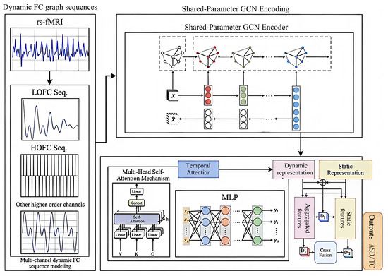
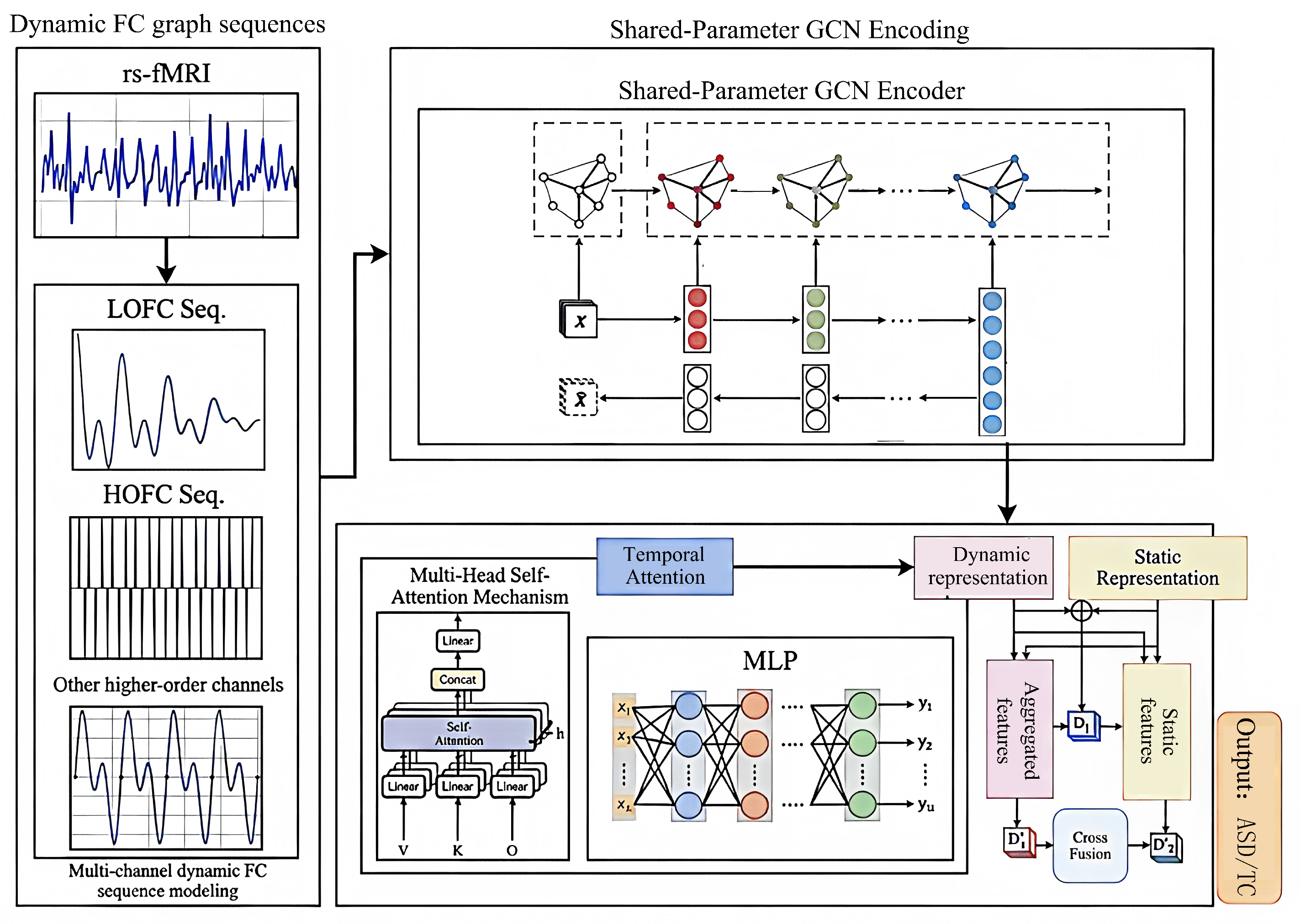
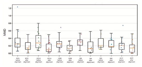
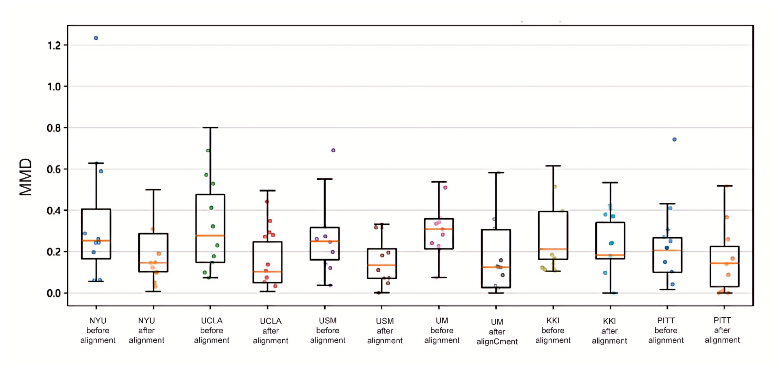
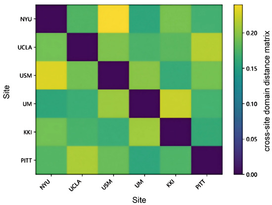
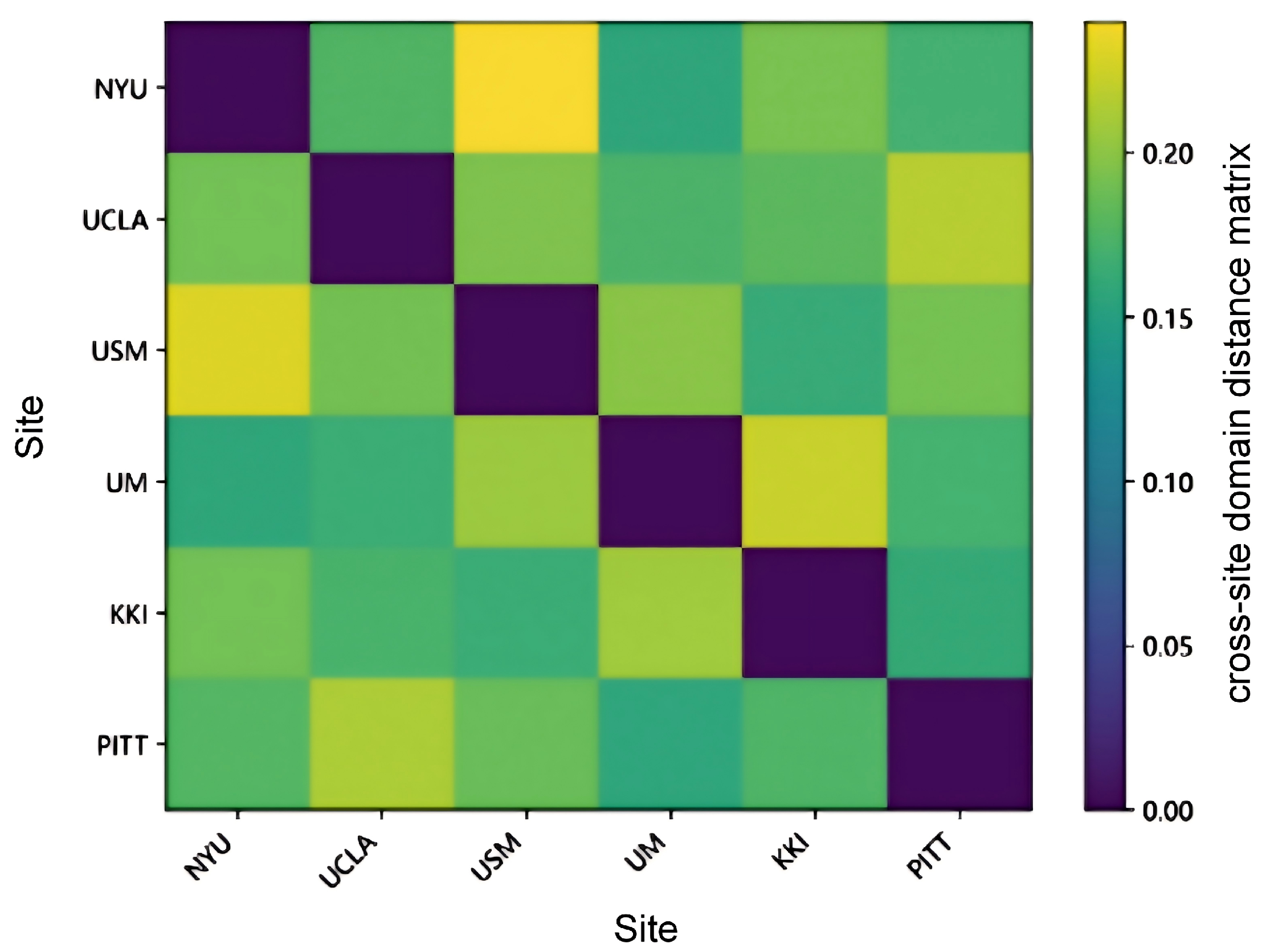
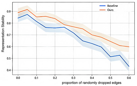
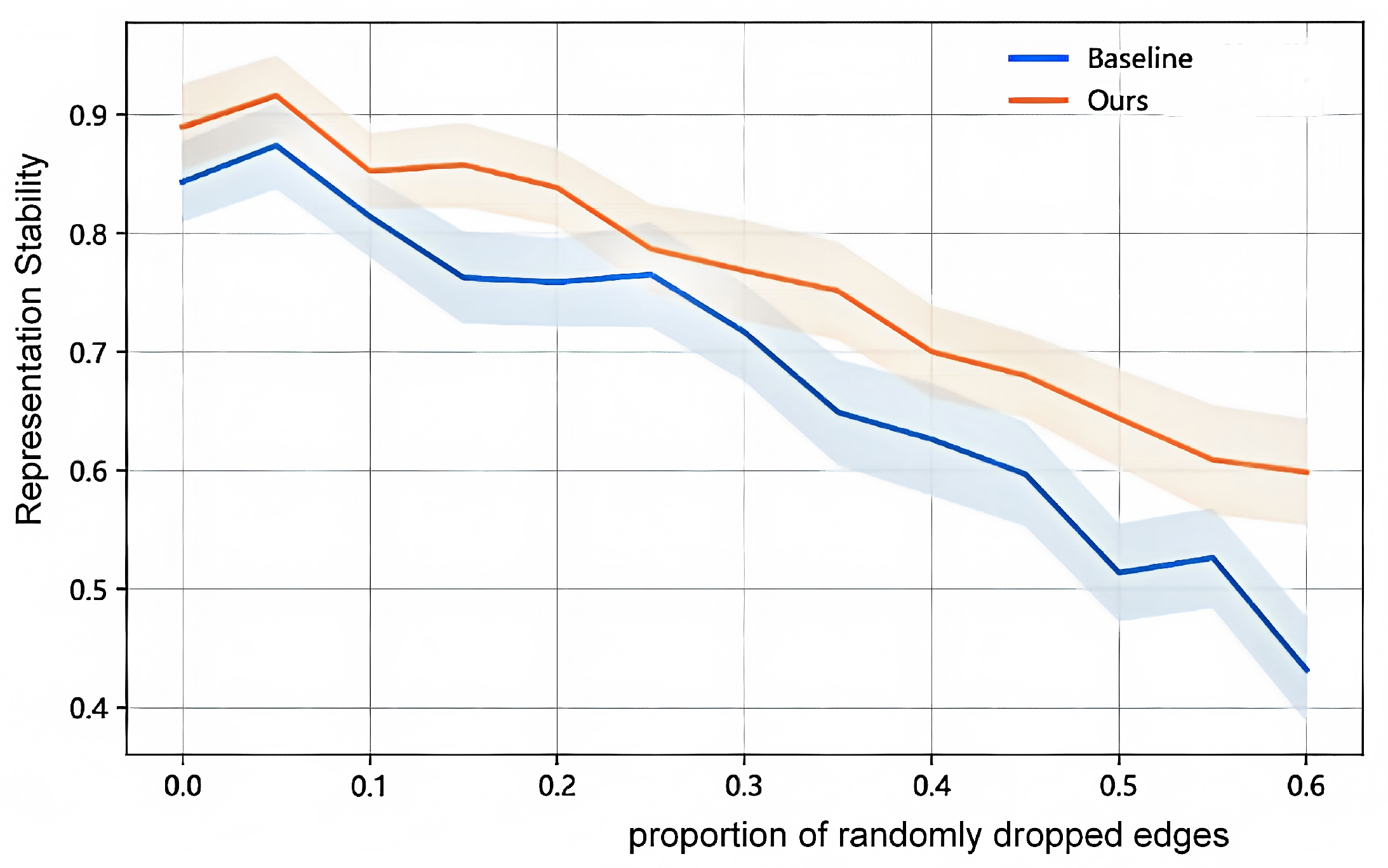
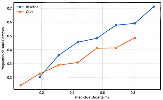
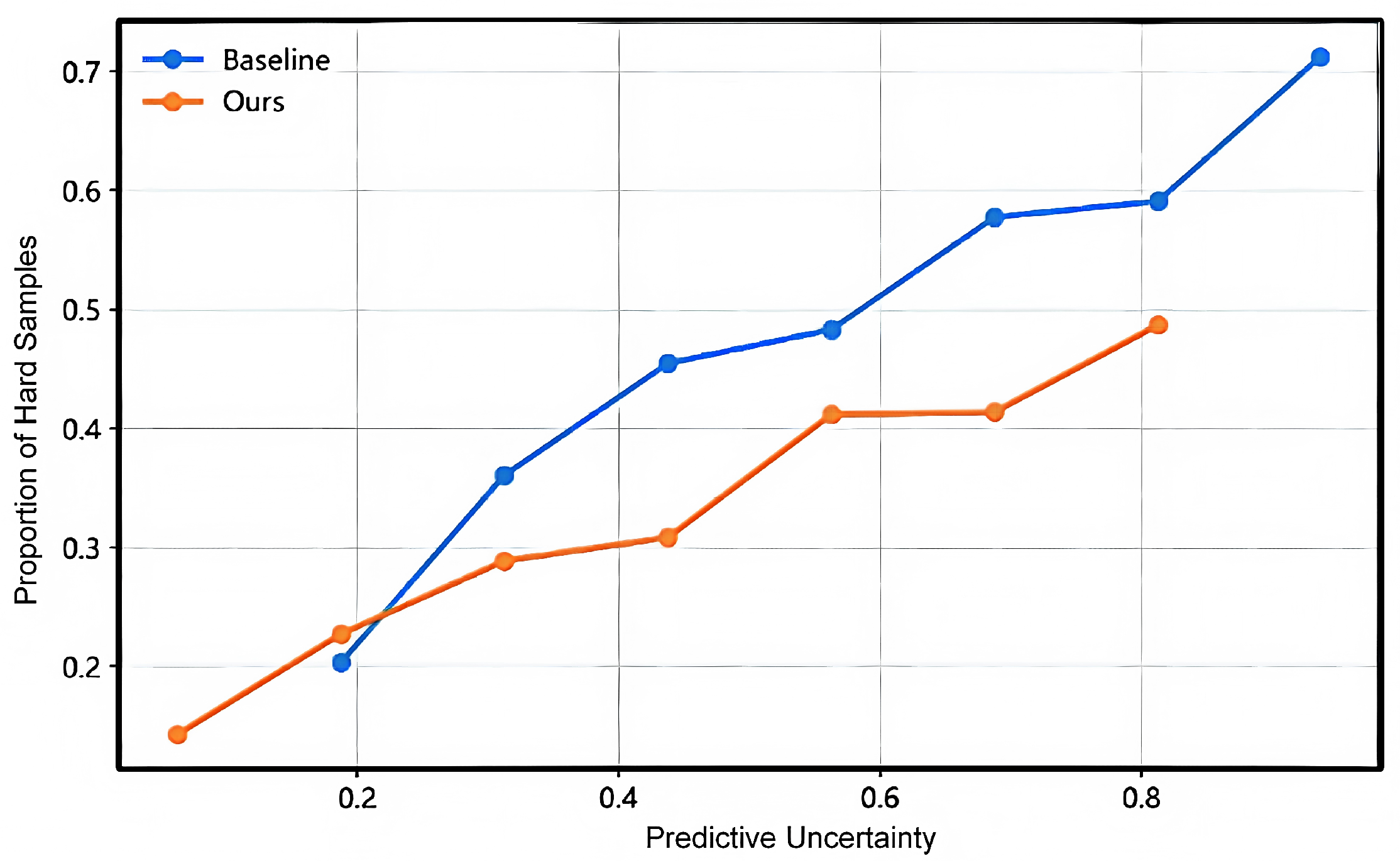
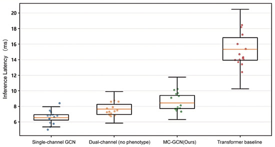
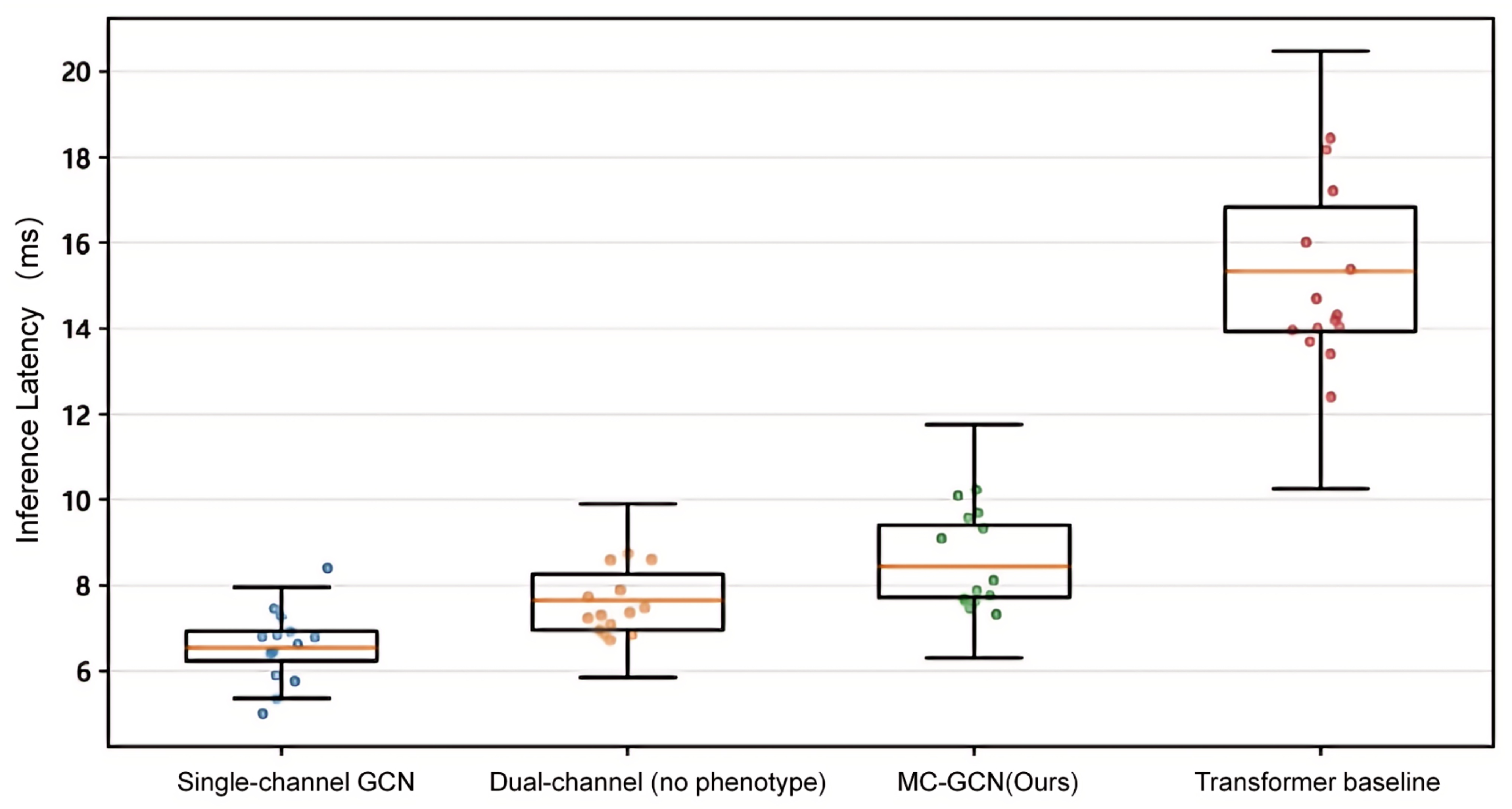
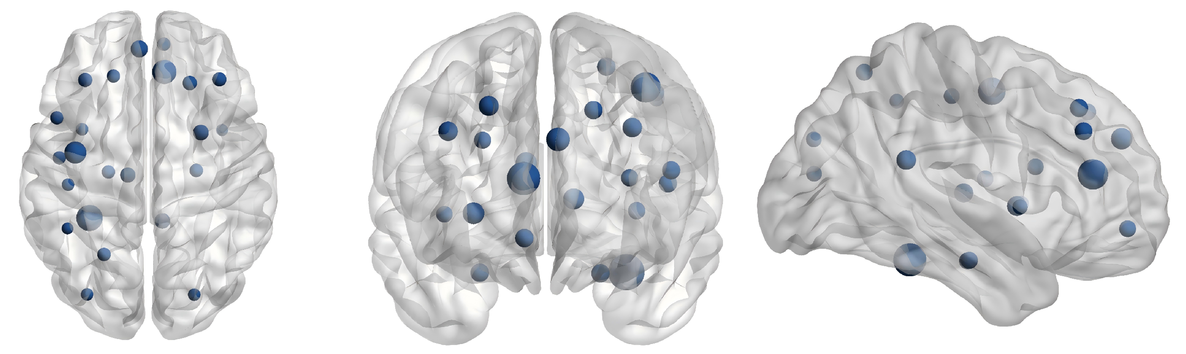

Disclaimer/Publisher’s Note: The statements, opinions and data contained in all publications are solely those of the individual author(s) and contributor(s) and not of MDPI and/or the editor(s). MDPI and/or the editor(s) disclaim responsibility for any injury to people or property resulting from any ideas, methods, instructions or products referred to in the content. |
© 2026 by the authors. Licensee MDPI, Basel, Switzerland. This article is an open access article distributed under the terms and conditions of the Creative Commons Attribution (CC BY) license.