


Abstract
Treeensembles usually evaluate every tree or boosting stage for every input, even when the partial prediction has already stabilized. We study inference-time lazy evaluation for pre-trained random forests and gradient-boosted decision trees. LazyRF stops random-forest evaluation using a Bayesian vote-stability score for the current leading class. LazyGBM uses a deterministic residual-capacity certificate: if the current class separation exceeds twice the maximum possible contribution of later stages, the final predicted class is guaranteed unchanged. At the default LazyRF threshold, LazyRF reduces evaluated trees by 60–90% across four benchmarks and 30 seeds while passing a paired-seed equivalence check with a 0.002 accuracy margin against full random-forest evaluation. For LazyGBM, the certified rule is conservative: certificate-only savings are 1–12% in the reported ablations, while more aggressive heuristic exits are reported separately and treated as empirically audited prototypes. We, therefore, use evaluated trees or stages as the main cost measure. Runtime measurements provide Python-prototype context rather than hardware-independent latency claims.
Keywords:
work-efficient inference; gradient boosted decision trees; instance-adaptive inference; random forests; sequential inference; stability thresholding; stopping rules; tree ensemble inference MSC:
60G40; 62L10; 68T05; 62F15
1. Introduction
Tree ensembles, especially Random Forests (RF) and Gradient Boosted Decision Trees (GBDT), remain core building blocks in computational machine learning because they provide strong accuracy and robust behavior on structured data, and are widely supported by mature training toolchains [1,2,3,4]. Standard inference evaluates every tree or boosting stage for every input, giving a fixed per-example cost even when the partial ensemble prediction has already stabilized. This evaluate-all protocol motivates lazy evaluation: for easy inputs, a method may be able to stop after a prefix of the ensemble while retaining the full-model decision. The practical relevance of this reduction depends on the cost profile of the surrounding pipeline. Lazy evaluation is useful only when the ensemble-evaluation loop is a measured cost after data access, preprocessing, feature construction, distributed scheduling, and I/O have been accounted for. This condition appears in latency-sensitive services (e.g., fraud screening, ranking, and monitoring pipelines), in high-volume batch scoring, and in always-on services where repeated full-ensemble evaluation contributes to compute or energy use [5]. When pipeline overhead dominates, fewer evaluated trees need not reduce end-to-end latency. This paper, therefore, studies component-count reduction as a bounded algorithmic objective for fixed tree ensembles, not as a universal deployment-acceleration claim.
1.1. Ensemble Inference as a Sequential Process
Although an ensemble is typically presented as a static mapping , the inference procedure is naturally sequential and evolves as the individual base learners are evaluated and aggregated. Let denote a partial state after evaluating t components on input x. For RFs, can be the class-vote count vector, and for GBDTs, it can be the partial class-score (logit) vector. The state evolves according to:
where is the contribution of the -th component (a one-hot vote for RFs, an additive score increment for GBDTs), and T denotes the total number of components (trees or boosting stages). Conventional inference fixes the horizon to for every input, regardless of how quickly the partial state stabilizes.
1.2. Gap: Reducing Expected Work While Preserving Full-Model Behavior
Previous studies have accelerated ensemble inference in two ways. First, systems-level methods optimize tree traversal and memory layout to reduce constant factors (e.g., QuickScorer-style bitvector interleaving), but typically preserve evaluate-all-component semantics [6]. Second, conditional computation approaches, notably cascades and early-exit models, stop computation early based on confidence heuristics at pre-defined checkpoints [7,8]. Although effective in specific settings, these strategies often require additional training (for staged models or auxiliary exits) or impose coarse-grained checkpoints. More importantly, they do not directly provide a unified, model-preserving mechanism to quantify and tune fidelity relative to the deterministic prediction of a fixed, fully evaluated ensemble.
1.3. Our Approach: Fidelity-Targeted Stopping Rules with Explicit Stability Targets
This study targets inference-time lazy evaluation for pre-trained ensembles: evaluate components sequentially and stop early on an instance x once the current prediction is sufficiently stable with respect to the unevaluated remainder. The mathematical object of interest is a stopping rule whose cost is the number of evaluated ensemble components and whose fidelity target is agreement with a fixed full model. We use the fidelity-constrained stopping-rule objective formalized in Section 3.1 as a design lens: reduce the expected evaluated components while controlling disagreement with the full model under an explicit uncertainty model for the unseen suffix. We do not claim to compute the exact constrained optimum at serving time. Instead, the objective defines the fidelity target, and the implemented algorithms provide two types of practical evidence: a deterministic argmax-preservation certificate for boosting and empirically audited stability surrogates for RF and heuristic GBM exits.
Specifically, we develop two inference-time wrappers: (i) LazyRF for random forests, which uses a Dirichlet vote model together with a posterior-dominance score for the current leader; and (ii) LazyGBM for gradient boosting, whose mathematically certified component is a residual-capacity argmax certificate, with optional margin-based prototype heuristics reported separately and controlled at inference time.
1.4. Research Questions and Contributions
Guided by the above framework, we investigate three questions:
- 1.
- Can we derive instance-adaptive stopping rules for tree ensembles that substantially reduce the expected computation while providing explicit, quantitative stability surrogates tied to agreement with a full evaluation?
- 2.
- Can such stopping rules be applied as inference-time wrappers around the same fitted RF/GBDT models without modifying the learning procedure?
- 3.
- Empirically, how do the resulting methods compare to static cascades and early-exit baselines in the accuracy–efficiency trade-off across diverse datasets and random seeds?
In this paper, fidelity means matching the deterministic full-ensemble prediction, not necessarily the ground-truth label. A model-preserving wrapper is a test-time procedure that uses the same fitted ensemble rather than retraining or replacing it. This paper makes four contributions.
- 1.
- Full-model fidelity objective for lazy ensemble inference. We formulate partial ensemble evaluation through a constrained stopping objective: minimize expected work while bounding disagreement with the deterministic full-model prediction (Equation (2)). This formulation differs from standard early-exit and cascade objectives, which target ground-truth accuracy, confidence thresholds, or cost–accuracy Pareto curves. Our target is instead the reproducible output of a fixed, fully evaluated ensemble, giving the paper a narrow fidelity-to-full-model framing rather than a generic confidence-thresholding objective.
- 2.
- Random-forest vote-stability stopping. We introduce a Dirichlet posterior-dominance score (Equation (3)) that estimates, under an exchangeable Bayesian vote model, whether the current RF leader is stable. This score exploits the discrete vote structure of bagged forests, operates at tree-level granularity rather than fixed checkpoints, and provides an assumption-aware, continuously tunable stopping statistic. Prior cascade and early-exit methods for tree ensembles use confidence thresholds on raw vote fractions or fixed-checkpoint rules; the posterior-dominance score instead provides a conservative risk-screening statistic whose empirical accuracy–efficiency frontier is strong, without a claim of superior ordering over vote-share heuristics.
- 3.
- Certified GBM stopping with separated heuristics. We derive a deterministic early-stopping condition for additive boosting that preserves the full-model prediction (Proposition 1): if the current top-1 vs. top-2 margin exceeds twice the remaining capacity, the final argmax is guaranteed unchanged. This certificate is the main mathematical guarantee for LazyGBM and follows from additive score accumulation and explicit per-stage output bounds. We also give an expected-work bound (Proposition 2) showing that certificate savings depend on the distribution of the partial margin relative to the remaining stage capacity. We then evaluate optional margin-based heuristics as a separate prototype layer, providing practitioners with a transparent spectrum from certified full-model agreement to more aggressive empirically audited stopping.
- 4.
- Reproducible evaluation of work, fidelity, and calibration. Across four benchmarks and 30 random seeds, we report accuracy and work-unit reductions and characterize accuracy–efficiency trade-offs via threshold sweeps, within-family comparisons to static cascades, contextual early-exit neural references, runtime-context measurements, surrogate-calibration audits, stopping-time/work-quantile analyses, and component-level ablations that separate guaranteed from heuristic savings.
The resulting thesis is deliberately positive but bounded: the paper contributes a provably exact, label-free full-model agreement certificate for additive boosting, a strong reproducible empirical accuracy–work frontier for random forests, and an explicit separation between deterministic guarantees, assumption-aware stopping statistics, and heuristic stopping statistics.
1.5. Summary of Empirical Findings (And How to Interpret Them)
At the default LazyRF operating point , LazyRF reduces average evaluated trees from 100 to – (relative work reduction –) while keeping the displayed main-table accuracy change close to Full RF (rounded range ; Section 5.2); the paired-seed analysis reports a Higgs mean difference of while still passing the equivalence check. Aggregated over datasets, LazyRF evaluates work units on average (work reduction ) with a mean accuracy change of relative to Full RF (Section 5.2). LazyGBM should be read in three layers. Certificate-only is the certified guarantee. Certificate-plus-flip applies that certificate first and then permits an audited flip-score heuristic, so it is empirically audited rather than fully certified; Section 5.8 shows zero disagreement for both variants on Covertype and Higgs, and certificate-plus-flip on Higgs matches the current prototype at average work units with disagreement. The more aggressive default prototype reduces work by – and matches Full GBM accuracy on Credit Card and Higgs, but its Covertype and MNIST accuracy decreases ( and ) arise from exploratory heuristic behavior rather than from the certificate alone and fail the paired equivalence check in Section 5.3. In aggregate, the current LazyGBM prototype reduces work by with a mean accuracy change of relative to Full GBM (Section 5.2).
1.6. Scope of Claims
The central claim is an algorithmic reduction in the expected number of evaluated ensemble components under a stopping rule whose worst-case work remains bounded by full evaluation within the same model family. This form of lazy truncation is orthogonal to systems-level accelerators such as QuickScorer- or Treelite-style compiled traversal: those methods reduce the cost of evaluating a tree or a full ensemble, whereas the present rules decide how many components to evaluate for a given instance. For submission, this manuscript is intended as an original, non-concurrent article: no prior LazyRF/LazyGBM manuscript is reused here, and the contribution claimed in this paper is the combination of a fixed-ensemble fidelity formulation, a residual-capacity certificate for preserving the full-model prediction in additive boosting, and an explicit separation between deterministic certificates, assumption-aware RF stopping statistics, and optional GBM heuristics.
1.7. Paper Organization
The remainder of this paper is organized as follows. Section 2 reviews the relevant literature on cascades/early exits, systems-level ensemble inference accelerators, and sequential decision-making foundations. Section 3 presents the theoretical foundations and stability surrogates underlying stopping rules. Section 4 details the materials and methods, including the cost model, algorithms, and implementation choices. Section 5 reports the experimental results and threshold-sweep trade-offs. Section 6 discusses the implications, limitations, and threats to validity. Finally, Section 7 concludes the paper.
2. Related Work
This study lies at the intersection of conditional computation (stopping early on “easy” inputs), efficient execution of tree ensembles (reducing the cost per evaluated tree), production serving systems (meeting end-to-end latency/throughput constraints), and sequential decision-making (formalizing when additional evidence is no longer worth acquiring). We position our instance-adaptive lazy inference wrappers in these directions.
2.1. Static Cascades and Early-Exit Mechanisms
Cascaded classification originated in early vision systems, in which a sequence of progressively more expensive classifiers quickly filters out easy negatives [7]. The cascade paradigm has since been generalized to modern ML pipelines via learned two-stage cascades and anytime prediction frameworks [9], checkpointed ensembles, and routing rules, which allow inputs to terminate early when predictions are already confident. In deep networks, early-exit architectures attach auxiliary heads to intermediate layers. These heads apply entropy- or confidence-based exit criteria, enabling significant savings with limited accuracy loss [8]. Related studies have also explored specialized inference engines and compression-aware execution for neural models [10].
Our work shares the goal of reducing the expected inference cost, but differs in emphasis and deployment constraints. First, we targeted tree ensembles directly and preserved the trained model. LazyRF and LazyGBM are inference-time wrappers that do not introduce additional student models, exit heads, or gating networks. Second, instead of stopping at a small set of fixed checkpoints, we adapt the computation to a fine granularity (tree-by-tree for RF, stage-by-stage for boosting). Third, we explicitly tie early stopping to a stability surrogate—a computable certificate or bound/approximation to determine whether the current prediction can change when the remaining components are evaluated. This is a different design goal than standard confidence heuristics: the surrogate is intended to track the agreement with the full-model decision under the stated modeling assumptions (RF) or via deterministic residual-capacity reasoning (boosting).
2.2. Efficient Inference Algorithms and Compilation for Tree Ensembles
A complementary line of work reduces the constant factors of tree evaluation without changing the semantics of the full inference. QuickScorer accelerates scoring for additive ensembles via bitset-based traversal and cache-efficient rule evaluation [6]. Subsequent work further improves data-level parallelism and layout-aware execution; for example, RapidScorer maximizes compactness in data-level parallelization to speed up evaluation of large ensembles in latency-sensitive settings [11]. At the compilation level, Treelite converts tree ensembles (e.g., from XGBoost or LightGBM) into optimized C code by compiling decision rules into nested conditionals [12], and newer compilers like SilvanForge further optimize these schedules for modern hardware [13].
These methods primarily target the per-tree execution efficiency and typically evaluate all trees for every input. By contrast, our lazy inference schemes aim to reduce the number of evaluated components by stopping once the prediction is sufficiently stable with respect to the unevaluated remainder. Therefore, the two approaches are largely orthogonal and potentially composable. A production implementation can combine low-level tree execution accelerators with instance-adaptive truncation.
2.3. Fast Forest/GBDT Inference Libraries and Prediction Serving Systems
Recent work has emphasized end-to-end inference performance and deployability for decision forests in production. Guan et al. compared multiple end-to-end decision forest inference pipelines (e.g., ONNX-based runtimes, library-specific engines, and GPU-oriented backends) and highlighted that performance depends not only on kernel efficiency but also on data access patterns and surrounding data-management layers [14]. On the library side, Yggdrasil Decision Forests provides a C++-centric framework designed for both research and production, including serving and interoperability across language bindings [15].
Beyond tree-specific runtimes, prediction-serving systems address deployment concerns, such as batching, caching, model selection, and tail-latency control. Clipper introduced a general-purpose architecture for low-latency, high-throughput prediction serving across heterogeneous model frameworks [16], whereas TensorFlow-Serving provides a widely deployed serving stack with optimized model lookup and versioning mechanisms [17]. Recent work also explores compiling tree ensembles into tensor computations to leverage unified neural serving stacks [18]. At the pipeline level, InferLine focuses on provisioning and autoscaling multi-stage inference pipelines to meet stringent end-to-end latency objectives under varying loads [19]. These systems reduce end-to-end latency through batching, scheduling, compilation, layout, and hardware-aware execution. Our stopping rules address a different factor: for each instance, they decide how many components of the already-trained ensemble to evaluate while preserving a worst-case work bound equal to full evaluation within the same model family. In a production implementation, the realized latency would depend on both terms—the per-component cost supplied by the backend and the number of components retained by the stopping rule—as well as the overhead of evaluating the rule itself. In response to this deployment question, Section 5.6 adds native LightGBM/XGBoost predictor measurements as optimized full-model context, while Section 5.7 adds full-size targeted checks for TL2cgen compilation of the fitted scikit-learn GBM, an optimized LazyGBM traversal, compact retrained ensembles, and shallow-tree retrained ensembles under the four-dataset, 30-seed protocol. The native rows quantify what is available when model/backend substitution is allowed; the targeted compiled/compact/shallow rows answer fidelity and retraining questions, but they are still controlled CPU timing checks rather than deployed service benchmarks.
2.4. Sequential Analysis, Optimal Stopping, and Adaptive Computation
Sequential analysis provides classical tools for deciding, based on partial evidence, whether additional samples are needed to reach a decision with a controlled error. Wald’s sequential probability ratio test (SPRT) formalizes optimal (in an expected-sample sense) testing between simple hypotheses under type-I/II constraints [20]. More recent work revisits learning stopping policies for early classification under finite horizons and connects uncertainty quantification to stopping decisions [21].
More broadly, adaptive inference has been studied under adaptive computation and budgeted prediction, in which computation (or feature acquisition) is allocated per instance under explicit cost constraints. Adaptive Computation Time (ACT) learns a halting policy that dynamically allocates iterative computation to harder inputs [22]. Budgeted prediction frameworks learn gating or model-selection rules that approximate a high-cost model using cheaper surrogates on easy instances [23]; related cost-aware tree-ensemble variants have been studied for feature-acquisition budgets [24]. Our contribution is complementary: we keep a fixed, pre-trained ensemble and adapt inference by truncating the evaluation of its existing components, using stability surrogates designed to track agreement with the full-model decision.
Our setting differs from classical sequential testing in an important way: the “ground truth” decision we aim to match is the deterministic prediction of a fixed, fully evaluated ensemble. The uncertainty that enables probabilistic reasoning arises from modeling the unobserved suffix of the computation given the observed prefix (e.g., posterior-predictive uncertainty over unseen RF votes or bounded residual capacity for unseen boosting stages). Accordingly, we use the sequential perspective primarily as a design lens for stopping-time rules and thresholding rather than claiming to implement an SPRT-optimal procedure in the classical hypothesis-testing sense.
2.5. Positioning of the Present Work
Table 1 provides a structured comparison of the present work against the most directly related paradigms. To summarize the key differentiators, three axes jointly distinguish the present contribution from prior work:
Table 1.
Positioning of the present work against related adaptive-inference paradigms.
(i) No training modification. Cascades, early-exit networks, budgeted prediction, and anytime ensembles all require changes to the training procedure—staged training, auxiliary exit heads, learned gating networks, or reordered boosting sequences. By contrast, LazyRF and LazyGBM operate as post-hoc inference-time wrappers around an already-trained ensemble. This provides a model-preservation advantage for already-trained scikit-learn-style RF or GBM models because the wrappers do not require retraining, revalidation of a new model, or access to the training data.
(ii) Fine-grained, per-component stopping. Cascade and early-exit methods stop at a small, fixed set of pre-defined checkpoints (e.g., after 10, 50, or 100 trees). Our methods check the stopping condition at every block boundary (LazyRF, typically every trees) or every stage (LazyGBM, ), enabling the stopping time to adapt to each instance at the natural granularity of the ensemble. This fine granularity is what enables LazyRF to achieve 78% mean work reduction (Section 5.2) compared to 55% for the fixed cascade and 50% for the two-stage cascade at the same operating point.
(iii) Fidelity to the deterministic full-model prediction. Standard early-exit and cascade criteria target ground-truth accuracy (or a proxy thereof), meaning that the stopping rule is designed to be correct with respect to the true label. Our stopping criteria instead target agreement with the full-model prediction —a strictly different objective. This distinction matters because it enables a well-defined, verifiable fidelity guarantee: disagreement with the full model can be measured exactly on any dataset without labels, and the LazyGBM certificate (Proposition 1) provides a deterministic, zero-disagreement guarantee when triggered. Margin-vs.-remaining-budget arguments also appear in anytime boosting, including SpeedBoost [9]; the narrower contribution here is a full-model agreement certificate for fixed, pre-trained GBM inference, framed as fidelity to the full-model prediction rather than target-label loss.
This positioning is important for interpreting the experiments: the strongest fairness claims are within-family comparisons to fixed-evaluation or RF-cascade baselines, whereas cross-family comparisons to neural early exits are contextual rather than like-for-like.
3. Theoretical Foundations
This section makes the mathematical content explicit before the algorithms and experiments. The stopping-rule formulation in Equation (2) places the work–fidelity trade-off in the language of sequential analysis (MSC 62L10), while the LazyRF posterior-dominance score uses a Bayesian vote model (MSC 62F15). For additive boosting, Proposition 1 gives the main full-model agreement certificate, Corollary 1 gives its binary specialization, and Proposition 2 bounds expected certificate work through the distribution of partial margins relative to residual capacity. These statements connect martingale/filtration-style stopping-time notation (MSC 60G40) with algorithmic inference for machine learning (MSC 68T05).
3.1. Stopping-Rule View of Lazy Inference
Lazy inference treats test-time evaluation as a sequential decision process with an explicit stopping rule. We summarize the key notation used throughout this section in Table 2. Let denote the partially evaluated state after t components on input x (e.g., vote counts for RFs or partial logits for GBMs), and let be the natural filtration generated by . A stopping rule is a measurable mapping such that for all t.
Table 2.
Notation used in Section 3.
A canonical soundness objective is to minimize the expected work subject to a fidelity constraint relative to the full evaluation.
where is user-chosen. Because the full ensemble is deterministic, the probability in (2) is induced by an explicit uncertainty model for the unseen suffix conditional on the observed prefix. Solving (2) exactly is generally infeasible at serving time; instead, we derive computable stability quantities (probabilistic surrogates or deterministic certificates) whose thresholding yields practical, instance-adaptive stopping rules.
3.2. Random Forests as a Bayesian Vote Process
3.2.1. Posterior-Dominance Score Used by the Implementation
Consider a T-tree RF classifier, where tree i casts vote . After evaluating t trees, let be the vote count for class c, let be the current leader, and define Dirichlet posterior parameters with . The experimental LazyRF implementation reasons about a latent class-probability vector and uses the posterior-dominance score
as its stopping statistic.
3.2.2. How Is Approximated in Practice
Code-specific quantities used only by the optional GBM flip-score heuristic, including the squared suffix proxy , the auxiliary denominator , and the implementation score , are introduced later in the heuristic flip-score paragraph, Section 4.3, and Appendix A.
The quantity in (3) is not evaluated exactly for all K in the prototype. For , it reduces to the exact Beta posterior tail . For , the implementation uses Monte Carlo Dirichlet samples when the total posterior mass is small (), and otherwise uses a best-vs-runner-up Gaussian approximation. Let denote the current runner-up class. Under the Dirichlet posterior,
and
It is the same below: large-count approximation then becomes
where is the standard normal CDF. This score is monotone in posterior dominance, but it is not the exact finite-horizon probability that the partially evaluated forest will match the deterministic full-forest decision. In the Gaussian branch it is also a runner-up approximation rather than a full multiclass argmax probability. The Dirichlet vote model also treats the unevaluated votes through an exchangeable latent-probability view; correlated trees reduce the effective amount of independent vote evidence and can weaken the literal posterior interpretation. Accordingly, we interpret as an assumption-aware posterior-confidence score whose relation to actual full-model disagreement and forest diversity must be validated empirically. Section 5.9 provides that calibration audit.
3.3. Boosting as Additive Score Accumulation
A K-class gradient-boosted tree ensemble (with shrinkage) produces additive class scores
and predicts . Assume that a per-stage bound holds for all x (computable from tree leaf ranges). Define the remaining capacity,
Then any class score can increase by at most and decrease by at most over the unseen remainder, implying that
Proposition 1
(Lossless early stopping for boosting). If , then ; i.e., stopping at t gives the same label as full evaluation.
Proof.
Let . By the definition of , for every class c. For the current leader and any competitor ,
If , this difference is strictly positive for every competitor, so the stage-t leader remains the unique full-model argmax. Hence . □
Corollary 1
(Binary boosting certificate). For binary additive boosting, let denote the signed scalar margin after t stages, with prediction determined by the sign of under the fixed tie-break rule, and let bound the absolute remaining scalar contribution. If , then ; stopping at t gives the same label as full evaluation.
This is the binary specialization of Proposition 1: the unseen suffix can perturb the scalar binary decision margin by at most , so a margin whose absolute value already exceeds cannot cross zero. The multiclass certificate uses because a pairwise class margin can decrease by through the current leader and by another through a competitor.
Proposition 2
(Expected work of certificate stopping). Let X be drawn from the deployment distribution, and define the certificate stopping time
Then
Proof.
For any integer-valued stopping time supported on , . If , the certificate has not fired by stage t; in particular, the stage-t certificate condition is false, so . Therefore, for each , which gives the bound. □
This bound connects the deterministic certificate to expected component work without adding an experimental assumption. Large savings are possible when the margin law rapidly places most examples in the region for small t; savings are limited when the distribution of remains close to or below the residual-capacity threshold until late boosting stages. This formalizes the empirical observation that boosting saves less when later stages remain corrective.
Only this residual-capacity certificate is deterministic; the RF posterior-dominance score and the non-certificate LazyGBM exits are surrogates or heuristics whose fidelity must be assessed empirically.
3.3.1. Heuristic Flip Score Used in the Prototype
When are loose, the deterministic certificate can be conservative. The non-certificate LazyGBM branch, therefore, uses a monotone margin–capacity score that decreases as the current top-class margin grows relative to a squared suffix-capacity proxy,
The implementation score is
with a small numerical in the denominator. This score is not a probabilistic guarantee for deterministic GBM; it is an empirical margin–capacity heuristic whose behavior is audited in the experiments. The auxiliary Azuma–Hoeffding derivation that motivated its monotone form is given in Appendix A, but Proposition 1 remains the sole mathematical guarantee for LazyGBM.
The implementation uses the following stack:
- 1.
- Lossless certificate: stop if .
- 2.
- Multiclass ratio heuristic: in multiclass settings, stop if with .
- 3.
- Flip-score heuristic: if , stop when , with in multiclass and in binary.
- 4.
- Late-stage fallback: in multiclass settings only, once more than of stages have been evaluated, stop if the current top-1 margin is simply positive.
Only the first rule guarantees the same prediction as the full model. Rules (ii)–(iv) are prototype heuristics included to study a broader deployment frontier, and they are ablated explicitly in Section 5.8. Accordingly, the user parameter is an aggressiveness parameter for the heuristic flip score and not a certified or calibrated bound on in the deterministic model.
3.3.2. Summary
For RFs, the evaluated implementation uses a Dirichlet posterior-dominance score over the current leader rather than an exact finite-horizon full-forest agreement probability. For boosting, the additive structure provides a deterministic residual-capacity certificate together with a stack of margin-based heuristics whose aggressiveness is exposed to the user. Together, these mechanisms yield lightweight, instance-adaptive inference rules that leave training unchanged but must be interpreted through their empirical agreement with full evaluation.
3.3.3. Mathematical Scope and Assumptions
The formulation in (2) is a fidelity target for designing and evaluating stopping rules, not an online algorithm for solving the constrained optimization problem exactly. LazyRF instantiates this target through a Dirichlet-model posterior-dominance surrogate; the score is useful for thresholding but is not an exact full-forest agreement probability. LazyGBM contributes a deterministic full-model agreement certificate only when the residual-capacity condition is satisfied. Its ratio, flip-score, and late-stage exits remain empirical heuristics whose effect is quantified by the disagreement, sweep, and ablation results.
4. Materials and Methods
This section specifies the computational cost model and presents the inference-time procedures for LazyRF and LazyGBM. Both methods act as wrappers around a pre-trained ensemble: training is unchanged, and only test-time evaluation is truncated via an instance-adaptive stopping rule. Table 3 summarizes the guarantee status of each stopping quantity before the algorithmic details are introduced.
Table 3.
Guarantee and heuristic status of the stopping quantities used in this manuscript.
4.1. Cost Model and Work Units
We consider multiclass classification with input and label . The inference cost is measured in work units:
- Random Forest (RF): One work unit is one tree evaluation (one root-to-leaf traversal).
- Gradient Boosting (GBM): One work unit is a boosting stage (one boosting round added to the additive score).
Clarification (multiclass GBM): In scikit-learn, GradientBoostingClassifier treats one “stage” as one boosting round: a single tree for binary classification or K trees for K-class problems. Accordingly, the reported GBM work units should be interpreted as rounds. In the multiclass case, each round entails K tree traversals. Therefore, a full evaluation costs T (RF) or S (GBM rounds) work units per example. The lazy method evaluates the stopping time (RF) or (GBM), thereby incurring the expected cost . We report work units as the primary cost proxy because they are independent of a specific software backend; wall-clock timings additionally depend on language/runtime, vectorization, batching, and wrapper overhead. Comparability note: Work units are intended for within-family comparisons (RF vs. RF; GBM vs. GBM). Cross-family comparisons (e.g., RF vs. MLP) are qualitative.
4.2. LazyRF: Block-Wise Posterior-Dominance Stopping
LazyRF targets RF majority-vote inference. Let be the class vote from tree t. After evaluating t trees, we define the vote counts
and the current leader using a fixed deterministic tie-break rule.
4.2.1. Stopping Statistic
As derived in Section 3, the implementation computes the posterior-dominance score from Equation (3). For binary tasks, this is the exact Beta posterior probability that the current leader remains above . For multiclass tasks, the prototype uses Monte Carlo Dirichlet sampling while , and otherwise switches to the Gaussian approximation based on (4) and (5). We stop once for a user-chosen threshold . Because is a posterior-confidence proxy rather than an exact finite-horizon agreement probability, its fidelity is assessed empirically rather than claimed analytically.
4.2.2. Block-Wise Evaluation
To amortize the decision overhead, we evaluate trees in blocks of size B and check the stopping condition only at the block boundaries. Thus, the admissible LazyRF stopping times lie on the fixed grid ; if falls between two boundaries, the first eligible check occurs at the next boundary. This preserves the worst-case cost T while reducing the per-tree control-flow overhead. The complete LazyRF inference procedure is detailed in Algorithm 1.
| Algorithm 1 LazyRF block-wise posterior-dominance inference | ||
| Require: Input x; trained RF ; block size B; | ||
| threshold ; min trees ; prior (default ). | ||
| 1: | Initialize counts for . | |
| 2: | for do | |
| 3: | for to t do | |
| 4: | Evaluate vote and update . | |
| 5: | end for | |
| 6: | ▹ fixed tie-break | |
| 7: | if then | |
| 8: | for all c; . | |
| 9: | if then | |
| 10: | Compute exact Beta posterior: | |
| 11: | . | |
| 12: | else if then | |
| 13: | Estimate via Monte Carlo Dirichlet samples. | |
| 14: | else | |
| 15: | ||
| 16: | Compute and via (4) and (5). | |
| 17: | ||
| 18: | end if | |
| 19: | if then return and | |
| 20: | end if | |
| 21: | end if | |
| 22: | end forreturn and | |
4.2.3. Complexity
Updating the vote counts is . For binary tasks, the stop check is an exact Beta tail evaluation. For multiclass tasks, the small-count branch uses a fixed Monte Carlo budget, while later checkpoints use only runner-up selection and a Gaussian CDF evaluation. Thus, the per-checkpoint overhead is modest and independent of T.
4.2.4. Implementation Notes
(i) The Gaussian branch uses a fast tanh approximation to the normal CDF . (ii) The Monte Carlo branch is used only for small posterior masses; later checkpoints default to the cheaper Gaussian approximation. (iii) The method retains the fitted RF: the underlying forest is unchanged; LazyRF only adaptively chooses .
4.3. LazyGBM: Residual-Capacity Certificate with a Prototype Heuristic Stack
LazyGBM targets additive-score ensembles (GBMs). Its method has two explicitly separated layers: a deterministic certificate that preserves the full-model prediction when triggered, and optional prototype heuristics that trade additional work reduction for empirically measured disagreement risk. Let be the class-score (logit) vector after t stages, with full model . We define the current top-1 and top-2 classes
and margin .
4.3.1. Precomputable Per-Stage Bounds
For stage s, we define an bound on its (shrinkage-scaled) score contribution as
where is the leaf value vector for stage s and is the learning rate (absorbed into if the library stores shrinkage-scaled leaves). We precompute the suffix sums:
which can be stored in arrays and accessed in time per step.
4.3.2. Lossless Stopping (Deterministic Certificate)
As shown in Proposition 1, if then the final argmax cannot change and stopping gives the same prediction as the full model.
4.3.3. Additional Heuristics Used in the Prototype
When are loose, the lossless certificate can be conservative. The reported prototype, therefore, layers several margin-based heuristics on top of the certificate; these heuristic exits account for any savings beyond the certificate-only mode and are not part of the deterministic guarantee. First, it computes the implementation flip-score heuristic from Section 3,
and evaluates the stopping condition
where is the user-chosen stability threshold (implementation parameter spr_threshold) and is the flip-score scale (multiclass_flip_scale; default in multiclass and in binary). For the binary case (), this simplifies to
whereas in the multiclass prototype with the equivalent algebraic condition is
This implementation score is a heuristic margin–capacity rule; its behavior is validated empirically in the ablation tables. In the multiclass prototype, this score is combined with a margin-to-bound ratio heuristic and a late-stage positive-margin fallback. Under the reported default and the certificate-first control flow of Algorithm 2, the ratio branch is inactive in the reported experiments because any example satisfying would already satisfy the certificate. None of these heuristics is lossless; they are exposed and ablated because they delineate a broader deployment frontier, even though the reported default operating point is shaped by the flip-score heuristic and late-stage fallback rather than by the ratio branch. The full prototype procedure is summarized in Algorithm 2.
| Algorithm 2 LazyGBM prototype inference (certificate + heuristic stack) | ||
| Require: Input x; trained GBM stages with initializer ; precomputed ; minimum stages ; ratio threshold ; stability threshold ; flip-score scale ; late-stage fraction . | ||
| 1: | . | |
| 2: | for to S do | |
| 3: | . | |
| 4: | ; . | |
| 5: | . | |
| 6: | if then return and | ▹ lossless certificate |
| 7: | end if | |
| 8: | if and and then return and | ▹ ratio heuristic |
| 9: | end if | |
| 10: | if then | |
| 11: | if or then return and | ▹ flip-score heuristic |
| 12: | end if | |
| 13: | end if | |
| 14: | if and and then return and | ▹ late-stage fallback |
| 15: | end if | |
| 16: | end forreturn and | |
4.3.4. Binary Case
For , Corollary 1 gives the scalar lossless certificate (with a consistent definition of from (10)), and the implemented flip-score heuristic reduces to the binary simplification in Equation (11), namely . The factor differs from the multiclass rule because a binary decision is a single scalar margin perturbable by at most , whereas a multiclass pairwise margin can move by .
4.4. Shared Implementation Choices
4.4.1. Minimum Evaluation ()
Both algorithms enforce a minimum number of evaluated components before checking the stopping conditions to avoid brittle early exits when the evidence is insufficient. For LazyRF, this acts only as an eligibility gate on the fixed block-boundary checkpoint grid; it does not offset the grid itself.
4.4.2. Deterministic Tie-Breaking
All operations use a fixed, deterministic tie-break rule to ensure reproducibility and avoid oscillatory behavior near ties.
4.4.3. What Is (And Is Not) Guaranteed
LazyGBM in lossless mode is certified by Proposition 1. All other LazyGBM exits (ratio heuristic, flip-score heuristic, and late-stage fallback) are prototype heuristics rather than deterministic or calibrated probabilistic guarantees for deterministic GBM inference. LazyRF uses a posterior-dominance score under a Dirichlet vote model; this score is a tunable fidelity mechanism rather than an exact full-model agreement probability.
4.4.4. Recorded Outputs
For each inference method, we recorded (i) predictive metrics, (ii) average work units , and (iii) when enabled, per-example stopping traces such as and the stop reason. These recorded summaries support the stopping-time/work-quantile and ablation analyses reported later. Work units are emphasized because they abstract away library/runtime constant factors and isolate algorithmic reductions in the expected evaluation.
5. Experimental Results
This section empirically evaluates the proposed instance-adaptive inference wrappers for tree ensembles (LazyRF and LazyGBM) and compares them to representative baselines across four benchmark classification tasks. The results should be read as two evidence classes: certified component reduction when the LazyGBM residual-capacity certificate fires, and empirically audited heuristic stopping behavior when LazyRF surrogates or optional LazyGBM heuristic exits are enabled. We focus on (i) the accuracy–computation trade-off induced by adaptive stopping, (ii) comparisons to static cascades and early-exit neural baselines, and (iii) robustness across random seeds and stopping thresholds.
5.1. Experimental Setup
5.1.1. Datasets and Preprocessing
We evaluated four publicly available classification benchmarks: MNIST (10 classes, 70,000 images; flattened to 784 features), Covertype (7 classes, 581,000 source instances, 54 features), Higgs (binary, ∼11 M source events, 28 features), and Credit Card Fraud (binary, highly imbalanced, 284,000 source instances, 30 features). Dataset provenance, access URLs, and licensing notes are provided in Section 5.1.3. For MNIST, we use the standard train/test split and scale pixel intensities to . For tabular datasets, we use stratified random train/test splits (80/20) per seed and standardize features using statistics computed on the corresponding training split only. The reported experiments use the full MNIST train/test split. To keep runtimes manageable, the implemented loaders cap the three large tabular datasets before the 80/20 split: Covertype is randomly capped at 200,000 examples using the experiment seed, while Higgs and Credit Card are read with a 200,000-row cap from the source CSV before stratified splitting. Secondary train/test caps are supported by the harness for smoke tests but were not used for the main reported results.
5.1.2. Model Configurations
To make the empirical evaluation self-contained and reproducible, Table 4 summarizes the concrete model hyperparameters, early-exit settings, and baseline configurations used in all experiments. Unless otherwise stated, we used library defaults and varied only the random seed (which controls the tabular train/test split and model randomness). All models were trained once per dataset/seed, and no post-hoc tuning was performed to favor the proposed methods.
Table 4.
Model and baseline configurations used in the experiments. “Full” models define the same-family reference for work normalization. “Lazy” methods wrap the fitted full model without retraining. The “Role in evidence” column states the question each row answers; only the full-model references, model-preserving stopping rules, and same-family RF stopping baselines support the central stopping-rule comparison. (default) indicates library defaults.
5.1.3. Code, Data, and Environment
Code
We released the source code for data loading, model training, evaluation, backend comparisons, and table/figure generation at https://github.com/pz1004/lazy_inference (accessed on 26 June 2026). The experimental environment used Python 3.11.8 (Python Software Foundation, Wilmington, DE, USA). The Python packages used were NumPy 1.26.4, pandas 2.3.3, scikit-learn 1.8.0, SciPy 1.16.3, Matplotlib 3.10.8, PyTorch 2.9.0+cu128, Numba 0.63.1, LightGBM 4.6.0 (Microsoft Corporation, Redmond, WA, USA), XGBoost 2.1.4, Treelite 4.7.0, and TL2cgen 1.0.0. These are open-source software packages; no chemicals, reagents, devices, instruments, commercial cell lines, samples, or biological materials were used in this computational study.
Data
All datasets are public benchmarks. Covertype and HIGGS are distributed through the UCI Machine Learning Repository under CC BY 4.0; Credit Card Fraud is distributed on Kaggle under ODbL v1.0; MNIST is freely available for research and educational use, although no formal license is specified by the original distributors. The repository provides the code needed to reproduce the preprocessing and evaluation pipeline, and the source sizes and experimental caps are reported here.
- MNIST: Released by Yann LeCun, Corinna Cortes, and Christopher J.C. Burges; freely available for research and educational purposes, with no formal license specified by the original distributors.
- Covertype: UCI Machine Learning Repository. Donated by Jock A. Blackard and licensed under CC BY 4.0.
- HIGGS: UCI Machine Learning Repository. Donated by Daniel Whiteson and licensed under CC BY 4.0.
- Credit Card Fraud: Kaggle “Credit Card Fraud Detection.” Originally released by the Machine Learning Group at Université Libre de Bruxelles (ULB) and licensed under the Open Database License (ODbL) v1.0.
5.1.4. Models and Baselines
We use two evidence tiers. The first tier tests the central stopping-rule claim: if the fitted model family is held fixed, how many ensemble components can be skipped while retaining audited agreement or accuracy relative to the full model?
- RF stopping comparisons: Full RF, LazyRF, Fixed Cascade, and Two-Stage Cascade RF compare stopping policies within the RF family.
- GBM stopping comparisons: Full GBM and LazyGBM compare full boosting evaluation with lazy stopping on the same fitted GBM; certificate-only, certificate-plus-flip, and prototype LazyGBM variants are separated in the ablation analysis.
These rows are the fairness anchors because they preserve the model family and mainly change the inference-time stopping policy.
The second tier answers practical alternatives that a reader may reasonably consider before adopting lazy stopping:
- If all trees are still evaluated, QuickScorer-style evaluation indicates constant-factor runtime context rather than work-unit reduction.
- If the model class can change, BranchyNet gives a cross-family early-exit reference, but it changes the architecture, training procedure, and unit of computation.
- If the backend or implementation can change, native LightGBM/XGBoost predictors test replacement models, TL2cgen tests exact fitted-model compilation, and Optimized LazyGBM tests whether the Python LazyGBM stopping semantics survive a lower-overhead traversal.
- If retraining is allowed, Compact RF-50, Shallow RF-d10, Compact GBM-50, and Shallow GBM-d2 measure the speed–accuracy trade-off of smaller or depth-limited ensembles.
These second-tier rows are not fairness anchors for the central stopping-rule claims. They change the intervention being tested: the model family, training procedure, backend, implementation target, or deployment objective.
5.1.5. Stopping-Rule Configurations
Unless otherwise stated, all ensembles used the same base size within each family to isolate the inference-time control-flow effects. For LazyRF, we set the confidence threshold to , enforce a minimum number of evaluated trees to avoid pathological early exits, and apply the stopping check every B trees (block-wise inference), so the first eligible stop check is the first block boundary with . The default values are , , and . For LazyGBM, the main tables report the current prototype configuration described in Algorithm 2: deterministic certificate, multiclass ratio heuristic (; inactive under the reported control flow), flip-score threshold , multiclass flip-scale , late-stage fallback after , and . Section 5.8 additionally evaluates certificate-only and certificate-plus-flip variants, where certificate-plus-flip means certificate first, then the audited flip-score heuristic.
5.1.6. Evaluation Metrics and Cost Reporting
Predictive Performance
We report the test accuracy for all datasets. For Credit Card Fraud (highly imbalanced), we additionally compute AUROC and AUPRC from positive-class scores during evaluation and report the resulting 30-seed audit in Table 5. To keep the main accuracy–work tables uniform across datasets and model families, Table 6, Table 7, Table 8, Table 9 and Table 10 report accuracy only. The primary fidelity target is agreement with the full model’s predicted class; preserving probability-score rankings or calibrated scores is evaluated separately only for the imbalanced Credit Card Fraud audit.
Table 5.
Credit Card Fraud score-metric audit over 30 seeds. AUROC and AUPRC are reported as mean ± 95% CI from positive-class scores. QuickScorer preserves the Full RF scoring semantics in this audit and, therefore, matches the Full RF score metrics.
Table 6.
Main results by dataset and method. We report mean test accuracy (mean ± 95% CI), mean work units, and relative work reduction (Equation (12)) with respect to the corresponding full-model reference within the same family.
Table 7.
Aggregate performance pooled over all datasets and seeds. We report mean test accuracy (mean ± 95% CI), mean work units, and relative work reduction (Equation (12)) relative to the within-family full reference.
Table 8.
Paired seed-level accuracy and TOST equivalence reanalysis from existing summaries. Mean diff. denotes the lazy/reference accuracy difference. Disagree. denotes the logged disagreement rate against the full-model reference. TOST uses an absolute-accuracy margin of at .
Table 9.
LazyRF threshold sweep. controls the stopping aggressiveness; larger is more conservative. We report mean accuracy (mean ± 95% CI), average work units, and relative work reduction for . Mean ± 95% CI over 30 seeds.
Table 10.
LazyGBM stability-threshold sweep (). Here is the threshold applied to the heuristic margin–capacity score rather than a classical sequential-test statistic. The flat rows on Covertype, Credit Card, and MNIST are interpreted as a negative/robustness result: savings there arise primarily from non- exits, while Higgs shows the main -controlled work trade-off. We report mean accuracy (mean ± 95% CI), average work, and relative work reduction for . Mean ± 95% CI over 30 seeds.
Work-Unit Proxy
We report a backend-independent work-unit proxy: one work unit corresponds to evaluating one RF tree or one GBM boosting stage. For BranchyNet, it is the number of blocks executed. Let be the mean work unit per test example and the corresponding full-model value in the same family. We define relative work reduction as
We intentionally avoid labeling (12) as hardware-energy savings because hardware energy depends on implementation details (vectorization, caching, batching, etc.) not captured by tree/block counts.
Tail Behavior and Worst-Case Bound
Tail latency is a predictable concern in early-exit methods. In this paper, we report mean work units as a backend-independent proxy and make the worst-case explicit. For all lazy methods, the stopping time is capped by the ensemble size, so the worst-case work equals the corresponding full model, up to wrapper overhead. To complement the mean work proxy, Table 11 reports 30-seed means of capped p50/p90/p95 stopping-time work quantiles for the lazy methods together with mean runtime and the corresponding full-model latency baseline. These are work-quantile statistics, not latency-quantile measurements; we interpret the runtime measurements as implementation context rather than as deployment-time latency evidence.
Table 11.
Stopping-time work quantiles and Python-prototype runtime context under the 30-seed manuscript protocol.
5.1.7. Random Seeds and Statistical Protocol
All reported values were averaged over random seeds. Each seed induces (i) a train/test split (for tabular datasets), (ii) model training randomness, and (iii) evaluation. For each metric, we report the sample mean and standard deviation across the seeds. We computed 95% confidence intervals using the Student-t critical value:
When comparing a method to its full-model reference, we compute per-seed differences (e.g., in accuracy) to reduce the variance attributable to the split and training seeds; the main tables report absolute accuracies (mean ± 95% CI) alongside work measures. These intervals are descriptive summaries across random seeds and are not used as formal equivalence tests or as proof of no difference.
5.2. Overall Performance
Table 6 reports, for each dataset and method, the mean test accuracy (mean ± 95% CI), mean work units, and relative work reduction with respect to the corresponding full-model reference within the same family (Equation (12)). Table 11 complements these averages with stopping-time quantiles and runtime context for the lazy methods.
Across datasets, LazyRF consistently reduces expected work, achieving relative work reductions of – while its displayed main-table accuracy changes remain in the rounded range relative to the corresponding Full RF (Table 6); the paired analysis below reports the exact seed-level differences. Relative to the two RF-cascade baselines, it usually delivers the largest within-family work reduction at the chosen operating point. For LazyGBM, Section 5.8 gives the certificate/heuristic split: the certificate-based variants are the safer reading, while the current prototype recovers extra work at the observed cost of larger disagreement on Covertype and MNIST (see Figure 1 and Figure 2).
Figure 1.
Test accuracy by method on the four benchmarks, visualizing Table 6. Bars show mean accuracy over random seeds for tree-ensemble methods (Full RF, static cascades, LazyRF; Full GBM, LazyGBM) and neural baselines (Full and Early-Exit BranchyNet). Numerical values and confidence intervals are provided in Table 6.
Figure 2.
Average work units by method on the four benchmarks, visualizing Table 6. For tree ensembles this corresponds to the average number of trees evaluated per test example (normalized so that Full RF/GBM use 100); for BranchyNet it is the average depth in blocks (1–3). LazyRF and LazyGBM consistently reduce work relative to their full counterparts, with LazyRF providing larger savings than LazyGBM.
LazyGBM reduces the number of evaluated boosting stages (averaging 32% reduction for the current prototype; Table 7), but the achievable reduction is generally more modest than that for RFs, reflecting the sequential error-correction structure of boosting.
Compared with the early-exit neural baseline, the proposed lazy schemes provide an instance-adaptive mechanism for tree ensembles that preserves a strict worst-case upper bound equal to full inference within the same model family. Cross-family comparisons (e.g., RF vs. BranchyNet) should be interpreted cautiously because their work units correspond to different computational primitives.
For the highly imbalanced Credit Card Fraud task, the AUROC/AUPRC audit in Table 5 provides a complementary view to accuracy. LazyRF has the same rounded accuracy as Full RF in Table 6, but its positive-class score ranking is lower (AUROC/AUPRC vs. for Full RF) because its score is derived from the partial posterior state at stopping. This distinction is expected because the stopping objective targets full-model label agreement rather than preservation of the full-model score vector. The RF cascades show a similar score-metric trade-off, whereas QuickScorer matches Full RF because it evaluates the complete forest. LazyGBM closely tracks Full GBM in both AUROC and AUPRC, indicating that the LazyGBM early exits do not materially change minority-class ranking relative to the GBM reference at this operating point.
5.3. Paired Accuracy and Equivalence Reanalysis
To strengthen the conclusion-validity evidence without running new experiments, we reanalyzed the existing 30-seed summaries by pairing each lazy method with its same-seed full-model reference. For each dataset–method pair, we computed the signed accuracy difference (lazy minus full), a paired t-test against zero mean difference, and two one-sided tests (TOST) for equivalence with a margin of absolute accuracy. Table 8 reports the resulting seed-level reanalysis. This is a reanalysis of stored summaries, not a new model run. McNemar tests were not run because the retained summaries contain seed-level accuracies and disagreement rates, but not per-example full/lazy prediction pairs.
The paired analysis sharpens, rather than broadens, the claims. LazyRF satisfies the equivalence criterion on all four datasets, even where the paired t-test detects a small nonzero mean difference. This combination is not contradictory: with 30 paired seeds, a tiny mean difference can be statistically detectable while still lying inside the pre-specified practical equivalence margin. The current LazyGBM prototype satisfies the equivalence criterion on Credit Card and Higgs but fails it on Covertype and MNIST, matching the interpretation that those two accuracy decreases come from heuristic exits beyond the certificate. In the Covertype/Higgs ablation summaries, both certificate-only and certificate-plus-flip LazyGBM preserve zero logged disagreement and pass the equivalence check; this supports the certificate-first reading while leaving per-example McNemar analysis to future retained-prediction analyses.
5.4. Threshold Sweeps
For LazyRF, we sweep to trace the empirical accuracy–efficiency frontier (Table 9). For LazyGBM in tunable mode, we sweep (Table 10). With all other hyperparameters and data splits held fixed, these sweeps provide two distinct checks: LazyRF shows the intended threshold-controlled frontier, whereas the LazyGBM sweep is mainly a robustness/negative result because several datasets are governed by non- exits.
The LazyGBM sweep should, therefore, not be read as a uniformly smooth frontier. Covertype, Credit Card, and MNIST are effectively flat over the swept range, indicating that their work savings under the current prototype come from exits outside the flip-score threshold. Higgs is the informative -controlled case: increasing makes the flip-score rule more conservative, moving average work from to while leaving mean accuracy unchanged at the displayed precision.
5.5. Stopping-Time Distribution and Runtime Context
The stopping-time quantiles sharpen the interpretation of the work proxy. Because Table 11 reports 30-seed means of per-seed quantiles, we use it to complement rather than replace the mean work results in Table 6. For easy datasets such as Credit Card and MNIST, LazyRF exits early for most examples, so the p50 and p90 work are far below the full-forest budget. Higgs is more difficult: the LazyRF p90 and p95 work remain at the full-forest budget, consistent with the smaller mean work reduction in Table 6. For LazyGBM, Covertype and MNIST consistently exit at 81 stages under the current multiclass prototype, Credit Card exits around 32 stages, and Higgs retains a high-work tail (p90 , p95 ), indicating that a substantial subset of Higgs examples still requires most boosting stages.
The runtime columns in Table 11 also explain why work reduction alone is not enough to claim deployment latency improvement. In this Python prototype, library-backed full-model inference is often faster in wall-clock time than the lazy wrappers despite their lower work counts, because stopping decisions introduce Python-level control flow and bookkeeping overhead. This is why we treat work units as the primary algorithmic evidence and runtime as contextual, implementation-dependent evidence.
5.6. Native Optimized-Backend Context
Native LightGBM and XGBoost answer the replacement-model question: if the fitted scikit-learn GBM does not have to be preserved, how fast are optimized full-model predictors under the same four-dataset, 30-seed protocol? Table 12 reports this context. These rows quantify the option available when replacing and validating the model/backend is acceptable; they do not compile the fitted scikit-learn GradientBoostingClassifier, preserve that fitted object, or implement LazyGBM stopping.
Table 12.
Native optimized-backend runtime context over the same four-dataset, 30-seed protocol.
Under this replacement-model interpretation, the native rows sharpen the decision boundary. XGBoost native prediction is faster than the scikit-learn Full GBM reference on all four datasets in this protocol (–) and faster than the Python LazyGBM wrapper by –. LightGBM native is faster than the Python LazyGBM wrapper (–) but slower than the scikit-learn Full GBM reference on these datasets (–). Accuracy also changes because the native rows are separately trained models: XGBoost improves Credit Card accuracy but is lower on Covertype and MNIST, while LightGBM improves MNIST but is lower on the three tabular datasets. Thus, if substitution and revalidation are acceptable, a native predictor may be the simpler deployment choice. If exact preservation of the fitted scikit-learn ensemble is required, these rows are not drop-in substitutes and are not evidence that LazyGBM itself is faster.
5.7. Compiled, Optimized-Lazy, and Retrained-Model Context
The next two context tables answer three follow-up questions that the native-backend table does not answer. First, can the fitted scikit-learn Full GBM be compiled without changing its test predictions? Second, can LazyGBM’s stopping semantics be preserved while reducing Python-wrapper overhead? Third, what speed–accuracy trade-off is obtained by retraining smaller or shallower ensembles? These rows follow the context-row interpretation in Section 5.1.4: they test fidelity or substitution under the manuscript’s dataset/seed protocol, not deployed-service latency. Table 13 is backed by 840 timing rows (four datasets × 30 seeds × seven selected methods) and 240 fidelity-check rows for the compiled and optimized-lazy checks. Table 14 summarizes a 720-row retrained-alternative analysis, combining verified full/compact rows with 240 additional shallow-tree rows for Shallow RF-d10 and Shallow GBM-d2. MNIST uses the full 60,000/10,000 train/test split; Covertype, HIGGS, and Credit Card use the existing 200,000-row caps before splitting, matching the manuscript data protocol. Training or compilation time is reported separately.
Table 13.
Full-size targeted compiled and optimized-lazy context over the four-dataset, 30-seed manuscript protocol.
Table 14.
Full-size targeted retrained model-alternative context over the four-dataset, 30-seed manuscript protocol.
The fidelity gates passed on all full-size targeted checks. TL2cgen compilation of the fitted scikit-learn Full GBM had zero test-set disagreement in 120/120 dataset-seed checks, so the corresponding rows in Table 13 can be read as exact fitted-model compilation for those test splits. The optimized LazyGBM implementation matched the Python LazyGBM wrapper in predictions, average work, per-sample evaluated-stage counts, and stop reasons in 120/120 checks. Its value is that the Python wrapper semantics can be preserved while reducing wrapper overhead: it is – faster than the Python LazyGBM wrapper. Relative to the scikit-learn Full GBM reference, however, Optimized LazyGBM ranges from –, so it is faster on Credit Card but slower on Covertype, HIGGS, and MNIST. TL2cgen compiled Full GBM is – faster than scikit-learn Full GBM and remains a full-model method, not a lazy stopping rule.
The retrained rows in Table 14 make the model-substitution alternatives explicit. Compact RF-50 reduces the estimator count by half and gives – prediction speedups, with accuracy deltas from approximately to . Shallow RF-d10 keeps 100 estimators but limits depth; it is faster (–) but its accuracy cost is dataset-dependent, ranging from approximately on Credit Card to on Covertype. Compact GBM-50 gives – speedups, with accuracy deltas from approximately to . Shallow GBM-d2 gives smaller speedups (–) and accuracy deltas from to . These rows do not use the same fitted model and should not be compared to LazyRF/LazyGBM as the same intervention: they answer what happens when a smaller or shallower model is retrained and revalidated, not whether an already validated full ensemble can be evaluated adaptively without retraining.
5.8. Ablation Studies
These 30-seed ablation tables (Table 15 and Table 16) clarify which design choices matter most. For LazyRF, smaller block sizes recover additional work savings because they allow more frequent stop checks. Under the fixed block-boundary implementation, acts only as an eligibility gate on that grid: with , the and rows coincide because both first check at 10 trees, whereas delays the first eligible check to 20 trees and is, therefore, more conservative. Larger block sizes also matter substantially: moving from to skips the 10-tree checkpoint altogether and increases average work on both Covertype and Higgs.
Table 15.
Mean over 30 seeds for LazyRF ablation results on Covertype and Higgs. Disagreement is measured against Full RF.
Table 16.
Mean over 30 seeds for LazyGBM ablation results on Covertype and Higgs. Disagreement is measured against Full GBM; work units are boosting rounds.
For LazyGBM, the certificate-only variant is the most conservative by construction, but the effect of the additional heuristics is dataset dependent. On Covertype, certificate-plus-flip recovers only a small amount of work relative to certificate-only, and both remain much more conservative than the current prototype. The logged stop fractions show that the ratio branch is inactive at the reported default and that flip-score exits are negligible on Covertype, so the remaining gap to the current prototype is attributable almost entirely to the late-stage fallback. On Higgs, certificate-plus-flip already matches the current prototype, so the flip-score heuristic appears to account for nearly all of the observed savings. These results are important for interpretation: the main-table LazyGBM numbers are not attributable to the lossless certificate alone. The LazyGBM heuristic stack is, therefore, supported by threshold sweeps, full-model disagreement rates, and targeted Covertype/Higgs ablations rather than by a calibration-style probabilistic guarantee.
5.9. Surrogate Validation and Calibration
A natural question is whether the LazyRF stopping score is empirically predictive of full-model disagreement (i.e., the event that early stopping changes the deterministic full-forest prediction). To validate this, we record for each test example the stopping-time score used by LazyRF and mark an example as a flip if the lazy prediction disagrees with the corresponding Full RF prediction. Table 17 summarizes 30-seed mean calibration statistics across all four datasets, and Figure 3 reports a reliability-style diagram on Covertype using 20,000 randomly sampled test examples from representative seed 42.
Table 17.
Mean over 30 seeds for cross-dataset LazyRF calibration summary. ECE is the expected calibration error between binned mean risk proxy and observed flip rate; Monotone seeds counts the seeds whose binned observed flip rates are nondecreasing with risk.
Figure 3.
LazyRF surrogate calibration on Covertype (20,000 test examples, representative seed 42). We bin examples by the predicted flip-risk proxy (quantile bins) and plot the observed flip rate (disagreement with Full RF) in each bin. The surrogate is used as a practical monotone stopping statistic and should not be interpreted as a calibrated posterior probability.
The calibration evidence is informative but heterogeneous. On Covertype, the 30-seed mean risk proxy is , whereas the observed flip rate is ; the proxy is, therefore, conservative on average, but the mean rank correlation is weak () and no seed satisfies the monotone-seeds check in Table 17. MNIST shows the same low-disagreement pattern (mean flip rate vs. mean risk proxy ), but only seeds satisfy this check. Credit Card remains effectively degenerate at the chosen operating point: the mean observed flip rate rounds to zero, the mean proxy is , and seeds satisfy the check, but the event rate is too small to support strong calibration claims. Higgs is the hardest case: the proxy is again conservative on average (mean proxy vs. flip rate ), but the mean Spearman correlation is extremely weak () and no seed satisfies the monotone-seeds check. We, therefore, treat only as a dataset-dependent stopping statistic that can provide conservative risk screening, not as a uniformly calibrated or strongly ordered per-example flip-probability estimate.
5.10. Summary of Findings
Overall, the experiments support one central claim and two decision boundaries. The central claim is that lazy stopping within the same model family can reduce expected evaluated components while keeping the lazy prediction close to the full-model prediction; the strongest evidence is LazyRF under the paired-equivalence checks. The first boundary is LazyGBM: certificate-only is the certified floor, certificate-plus-flip is a certificate-first heuristic variant with zero logged disagreement in the Covertype/Higgs ablations, and the full prototype remains exploratory. The second boundary is deployment: if a user can replace, compile, optimize, or retrain the model, the context rows describe those alternatives rather than extending the central stopping-rule claim.
6. Discussion
This section synthesizes the empirical findings through the lens of the research questions, clarifies the scope of the results, and delineates limitations, threats to validity, and actionable directions for future work.
6.1. RQ1: How Much Work Can Be Eliminated Without Materially Degrading Accuracy?
Across the evaluated benchmarks, LazyRF provides the largest (or tied-largest) work savings among RF-family methods at the operating point used in Table 6, reducing expected work by – while remaining inside the paired equivalence margin. The gains are largest on Credit Card and MNIST, where the stopping-time quantiles in Table 11 show that most examples exit very early, and smaller on Higgs, where a larger fraction of examples remain near the full-forest budget. For LazyGBM, the ablation rows separate the certified certificate-only rule from heuristic additions; the current prototype adds exploratory exits to recover more work. This pattern is consistent with later boosting stages remaining important on some examples even when the partial margin appears stable.
6.2. RQ2: How Do the Lazy Methods Compare to Static Cascades and Early-Exit Neural Baselines?
Relative to static cascades, LazyRF typically achieves larger work reductions at comparable accuracy; e.g., on Covertype and MNIST it reduces work by and versus and for the fixed cascade, while changing accuracy by at most and relative to the fixed cascade (Table 6). These are the fairest baseline comparisons in the paper because all methods remain in the RF family and differ mainly in inference policy rather than model class or training procedure.
The remaining rows answer different engineering choices, so they should not be read as additional stopping baselines for the same fitted ensemble. QuickScorer asks what constant-factor speedup is possible when all trees are still evaluated. BranchyNet asks how a cross-family early-exit neural model behaves under a different architecture and training objective. Native LightGBM/XGBoost ask whether backend/model replacement is preferable when revalidation is allowed. TL2cgen and Optimized LazyGBM ask whether exact compilation or lower-overhead same-rule traversal is feasible. Compact and shallow retrained ensembles ask whether a smaller validated model is a better latency option. These comparisons are useful precisely because they change the deployment decision; they are not evidence that lazy wrappers dominate optimized serving systems or separately tuned cross-family models.
6.3. What Is Technically Novel Beyond Prior Art?
The high-level intuition that stable predictions can stop early is not new. The narrower contribution of this paper is to make that intuition operational for fixed tree ensembles under a full-model-fidelity target. Rather than learning a new gate, retraining a cascade, or optimizing ground-truth accuracy under a budget, the proposed rules ask whether the current partial ensemble prediction is likely or guaranteed to match the deterministic prediction of the same fully evaluated model. Three elements carry this contribution:
6.3.1. The Posterior-Dominance Stopping Statistic for RF
Prior RF cascade and checkpoint methods use raw vote-fraction thresholds (e.g., stop if the top class exceeds 90% of votes so far). The posterior-dominance score instead places a Dirichlet posterior over the latent class-probability vector and computes the posterior probability that the current leader is dominant under that posterior (Equation (3)). This makes a tunable, conservative risk-screening statistic that incorporates posterior uncertainty in the latent vote probabilities. The calibration analysis (Table 17) shows that the score is conservative on average but only weakly ordered on some datasets; accordingly, the practical contribution is the tunable statistic and the empirically observed accuracy–efficiency frontier, not a claim of uniform calibration, superior ordering over vote-share, or universal superiority over simpler vote-share heuristics.
6.3.2. The Lossless Residual-Capacity Certificate for GBM
Proposition 1 provides a deterministic, zero-disagreement early-stopping condition: if , the final prediction is guaranteed identical to the full model. The certificate uses the additive score structure of a fixed pre-trained boosting ensemble together with explicit per-stage contribution bounds; it is, therefore, a full-model agreement statement, not a confidence heuristic about the true label. This is related in spirit to margin-vs.-future-budget reasoning in anytime boosting [9], but the object certified here is agreement with the already-trained full ensemble. Proposition 2 further shows that expected certificate work is controlled by how quickly the partial-margin distribution moves above the residual-capacity threshold. Although the certificate is conservative when per-stage bounds are loose (as shown by the ablation in Table 16, where certificate-only yields only 1–12% work reduction), it provides a hard safety floor before any optional heuristic exits are considered.
6.3.3. The Fidelity-to-Full-Model Formulation
The constrained stopping objective in Equation (2) targets , where is the deterministic prediction of the full ensemble—not the ground-truth label. This target differs from standard cascade, early-exit, and budgeted-prediction objectives that are usually expressed in terms of ground-truth accuracy or a cost–accuracy Pareto curve. The practical consequence is that fidelity can be audited without labels: any deployment can log the disagreement rate by periodically running the full model on a sample, providing a label-free monitoring signal. This formulation also decouples stopping-rule evaluation from the model’s intrinsic accuracy, making the framework applicable even when labels are delayed, unavailable, or noisy.
6.4. RQ3: Robustness Across Thresholds and Random Seeds
Threshold sweeps reveal smooth and largely monotone operating frontiers for LazyRF: increasing reduces the aggressiveness of stopping, increasing work and slightly increasing accuracy (Table 9). The one-factor ablations in Section 5.8 sharpen this picture: smaller block sizes recover additional savings by checking more often, whereas changes the operating point only when it moves the first eligible checkpoint to a later block boundary. At , the and rows coincide, while is more conservative because it defers the first stop check to 20 trees. For LazyGBM, the flat rows on Covertype, Credit Card, and MNIST are a negative/robustness result: changing the flip-score threshold has no displayed effect because savings arise from non- exits. Higgs is the meaningful -controlled case, with relative work reduction moving from to as increases from to while accuracy remains unchanged at the displayed precision (Table 10). The ablation results further show that the certificate-only variant is the most conservative and that the extra heuristic savings are dataset dependent: on Covertype they come almost entirely from the late-stage fallback, whereas on Higgs the flip-score heuristic already recovers most of the gap to the current prototype.
6.5. Why Lazy Inference Helps (And When It Is Expected to Help Most)
The empirical pattern aligns with the margin-stability view of the ensemble prediction. For random forests, many instances become effectively “decided” early: as votes accumulate, posterior uncertainty about the latent dominant class contracts rapidly, so additional trees yield diminishing returns for a large fraction of the inputs. LazyRF operationalizes this by stopping when its posterior-dominance score exceeds a user-specified tolerance, thereby allocating more computation to ambiguous instances and less to easy ones. Consequently, datasets with a higher prevalence of high-margin instances are expected to admit larger savings, whereas datasets with substantial overlap between class-conditional distributions require more trees on average at a fixed fidelity target.
The RF interpretation depends on the vote model. The Dirichlet score is most natural when the remaining tree votes behave like exchangeable evidence about a stable class-probability vector. Real forests contain correlated trees because bootstrap samples, feature subsets, and shared predictive structure do not produce independent voters. Correlation effectively lowers the independent evidence content of the observed prefix, so the score should not be read as a calibrated posterior flip probability. This is why Table 17 reports both average conservativeness and weak rank ordering on some datasets. In practice, the statistic is expected to be more reliable for diverse, high-margin forests and less reliable when many correlated trees make similar errors or when class margins remain small.
For boosting, early termination is intrinsically more delicate because later stages are designed to correct earlier residual errors; therefore, informative contributions can persist deeper into the sequence. This explains why LazyGBM typically yields smaller and more variable work reductions than LazyRF under a global configuration (Table 6). It also explains why the most aggressive prototype settings are not uniformly benign: when later stages remain corrective on hard examples, heuristic exits can increase disagreement even if the mean work drops. In practice, boosting-oriented lazy inference benefits the most when the margin grows quickly for a substantial subset of examples or when tighter, instance-conditioned residual-capacity bounds can be obtained.
6.6. Practical Interpretation: Target Users and Alternatives
The deployment decision should start with a cost audit. Lazy evaluation is worth considering for teams that must preserve an already validated RF or GBM, can periodically audit full-model disagreement, and have measured ensemble evaluation as a material part of latency or batch-scoring cost after data access, preprocessing, feature construction, distributed scheduling, and I/O. A simple cost-decomposition rule is useful: if full ensemble evaluation is only a fraction f of end-to-end time, then even eliminating all ensemble work can reduce total time by at most f. Thus, when model evaluation accounts for only 5% of a pipeline, adaptive tree stopping cannot yield more than a 5% end-to-end gain; when model evaluation is a large batch-scoring cost and the fitted model cannot be replaced, the same work reduction can be operationally relevant. The present evidence is strongest for this model-preserving setting. It is weaker for pipelines where feature construction, network transfer, database access, or orchestration dominates, and it is unnecessary when an optimized full-model predictor already satisfies the required latency, throughput, and resource budget.
The effect sizes should, therefore, be read at the component-evaluation level. The reported savings are reductions in evaluated components (Equation (12)), not measured hardware energy consumption or hardware-independent latency gains. Wall-clock improvements in the present prototype can be attenuated, or even inverted, by Python-level control-flow and bookkeeping overhead, whereas the full-model baselines are implemented in highly optimized library code. The most reliable claim supported by the experiments is an algorithmic reduction in expected evaluated components, together with a worst-case component count bounded by full evaluation within each family.
Reducing ensemble size, limiting tree depth, retraining a compact model, or deploying optimized predictors are more direct choices when a new model or backend can be validated and the goal is end-to-end latency. The native-backend context supports this practical advice: XGBoost native is faster than the scikit-learn Full GBM reference by – and faster than the Python LazyGBM wrapper by – (Table 12), but the accuracy changes mean it is a replacement model, not a drop-in preservation mechanism. The full-size targeted checks sharpen the same point: TL2cgen preserves fitted Full GBM predictions in 120/120 checks, Optimized LazyGBM preserves Python LazyGBM semantics in 120/120 checks while still being slower than scikit-learn Full GBM on three datasets, and Compact RF-50/GBM-50 or Shallow RF-d10/GBM-d2 reduce runtime only by changing and retraining the model (Table 13 and Table 14). The shallow rows also show why this alternative cannot be assumed to be harmless: Shallow RF-d10 loses accuracy on Covertype and on MNIST, while Shallow GBM-d2 loses on Covertype and on MNIST. The proposed wrappers address the narrower case in which the existing fitted ensemble is the object to preserve. They expose an inference-time knob for trading average evaluated components against full-model disagreement. For RFs, the relevant knobs are , B, and (Table 9 and Table 15). For GBMs, the first decision is whether exact full-model agreement is mandatory: use certificate-only when it is; inspect certificate-plus-flip when the Covertype/Higgs ablation evidence is acceptable for the deployment; treat the full current prototype as exploratory because its additional savings come from heuristic exits.
6.7. Limitations and Threats to Validity
We grouped limitations using standard validity taxonomies:
Internal validity: (i) Timing comparisons are confounded by implementation asymmetry: optimized library inference vs. Python control flow in lazy wrappers. (ii) Any reimplementation-based baseline (e.g., QuickScorer in Python) should not be interpreted as representative of optimized systems. (iii) The native LightGBM/XGBoost measurements are separately trained full-model alternatives, while the TL2cgen, Optimized LazyGBM, compact-ensemble, and shallow-tree rows remain controlled CPU checks under the context-row interpretation defined in Section 5.1.4. (iv) The composability argument for LazyGBM is algorithmic: an optimized backend could exploit fewer evaluated stages, but the present evidence does not establish hardware-independent latency improvement. (v) LazyGBM behavior depends on the particular choice of residual-capacity bound and heuristic stack; different bounding strategies or heuristic thresholds may shift the trade-off.
Construct validity: (i) Accuracy alone may be insufficient for imbalanced tasks (e.g., fraud detection), where AUROC/AUPRC and cost-sensitive metrics better reflect utility. (ii) The work proxy (evaluated trees/stages) does not directly quantify hardware energy. (iii) We report stopping-time quantiles averaged over 30 seeds, but a fuller deployment study would still measure tail latency over repeated runs in an optimized implementation. (iv) The LazyRF posterior-dominance score is informative but not uniformly calibrated across datasets, so it should be interpreted as a practical stopping statistic rather than as a universal flip-probability estimator.
External validity: (i) The results are based on four datasets and may not generalize to other modalities (e.g., ranking, regression) or different data regimes (e.g., distribution shift). (ii) The experiments primarily used scikit-learn-style ensembles for the lazy methods that retain the fitted model; transferring the stopping rules to widely deployed toolchains (for example, XGBoost/LightGBM) would require adaptations to handle residual bounds, traversal overhead, and backend APIs. (iii) The context rows add native backend, compiled backend, optimized-lazy, compact-model, and shallow-model evidence, but they still do not evaluate tuned hyperparameter searches or deployed service benchmarks.
Conclusion validity: The paired seed-level tests and TOST equivalence reanalysis in Section 5.3 reduce uncertainty about practically negligible accuracy differences using the stored 30-seed summaries. The remaining limitation is per-example agreement testing: McNemar tests require retained full/lazy prediction pairs, which were not available for this revision.
6.8. Future Work
Several directions follow directly from the empirical findings and the above limitations: (i) extending the TL2cgen and Optimized LazyGBM checks to additional datasets, model sizes, tuned hyperparameters, and serving stacks; (ii) integrating LazyRF/LazyGBM into optimized inference stacks (vectorized/compiled implementations) to translate work savings into consistent wall-clock reductions; (iii) implementing the stopping rules inside modern boosted-tree toolchains, rather than only benchmarking native full-model alternatives, and investigating tighter, instance-conditioned residual-capacity bounds to improve LazyGBM savings while controlling disagreement risk; (iv) extending task-appropriate analyses for imbalanced problems beyond AUROC/AUPRC to expected cost and assessing whether early stopping disproportionately affects minority-class behavior; (v) measuring deployment tail latency in optimized implementations and relating latency quantiles to stopping-time and margin distributions; (vi) evaluating robustness under distribution shift and auditing whether adaptive stopping induces systematic differences in compute allocation across subpopulations.
7. Conclusions
We studied instance-adaptive lazy inference for tree ensembles as an inference-time wrapper that truncates the evaluation of a fixed, pre-trained model. The central idea is to treat ensemble inference as a sequential process and stop when the current prediction is sufficiently stable with respect to the unevaluated remainder. The stopping objective defines the fidelity target relative to the deterministic full model; the practical contribution is a set of computable stopping quantities that can be evaluated online with modest additional bookkeeping.
We presented two concrete instantiations:
- LazyRF models the observed RF votes with a Dirichlet posterior and stops according to a posterior-dominance score for the current leader. The resulting threshold is an interpretable conservativeness knob, and the calibration audit clarifies its dataset-dependent behavior.
- LazyGBM uses the additive boosting structure to derive a deterministic residual-capacity certificate, whose binary specialization is given in Corollary 1 and whose expected-work implication is given in Proposition 2. The certificate-only mode is the conservative safety floor; certificate-plus-flip is a certificate-first, empirically audited variant that adds the flip-score heuristic; and the full current prototype is exploratory.
Across four classification benchmarks and random seeds, LazyRF reduced expected work by 60–90% at (relative work reduction –), with displayed main-table accuracy changes in and paired seed-level equivalence under the margin. For the current prototype at the default operating point, LazyGBM reduced work by 19–68%, passing paired equivalence on Credit Card and Higgs but failing it on Covertype and MNIST; the stronger and cleaner LazyGBM claim is, therefore, the separated certificate-first evidence rather than the prototype alone.
The additional analyses clarify when this claim should and should not be used. Stopping-time quantiles show that LazyRF savings are concentrated on easy inputs, while harder settings such as Higgs retain a high-work tail. The calibration audit shows that the LazyRF stopping score is useful but dataset-dependent. The LazyGBM ablations separate certified stopping from more aggressive heuristic exits.
The backend and model-alternative analyses define the decision boundary. If deployment can replace the fitted model, native predictors or retrained compact/shallow ensembles may be simpler choices. If exact fitted-model behavior must be retained, TL2cgen gives a compiled full-model option when zero-disagreement checks pass. If the LazyGBM stopping rule itself must be retained, the optimized LazyGBM rows test whether the same semantics can be run with lower wrapper overhead. The lazy wrappers target the narrower case in which the existing fitted ensemble remains the object to preserve and average component evaluation is still a measured cost.
The methods, therefore, provide interpretable control knobs ( for LazyRF and a certificate/variant/threshold configuration for LazyGBM) for settings in which average component evaluation remains a measured cost. The strongest supported claim is narrow: the methods reproducibly reduce the expected number of evaluated ensemble components, with explicit evidence about where each stopping rule is reliable, conservative, or heuristic. The RF score depends on modeling assumptions, the GBM prototype includes heuristic exits beyond the deterministic certificate, and the Python runtime context does not establish hardware-independent latency or energy reduction. Within those boundaries, the study establishes a practical route to adaptive computation when the fitted tree ensemble must be retained.
Author Contributions
Conceptualization, S.J., S.W. and A.L.; methodology, S.J.; software, S.J.; validation, S.J., S.W. and A.L.; formal analysis, S.J.; investigation, S.J., S.W. and A.L.; resources, S.J. and A.L.; data curation, S.J.; writing—original draft preparation, S.J.; writing—review and editing, S.W. and A.L.; visualization, S.J.; supervision, S.W. and A.L.; project administration, S.W. and A.L. All authors have read and agreed to the published version of the manuscript.
Funding
This research received no external funding.
Data Availability Statement
The data presented in this study are openly available at https://github.com/pz1004/lazy_inference (accessed on 26 June 2026).
Conflicts of Interest
The authors declare no conflicts of interest.
Abbreviations
The following abbreviations are used in this manuscript:
| ACT | Adaptive Computation Time |
| GBDT | Gradient Boosted Decision Tree |
| GBM | Gradient Boosting Machine |
| RF | Random Forest |
| SPRT | Sequential Probability Ratio Test |
Appendix A. Auxiliary Flip-Score Motivation
This appendix records the auxiliary concentration argument that motivated the monotone form of the LazyGBM flip-score heuristic. It is not used as a deterministic guarantee in the deployed method. The deterministic guarantee for LazyGBM is only Proposition 1.
For this motivation, define
Fix the current leading class under the fixed tie-break rule, and for each competitor define the stage-t margin
For , define the per-stage margin increments
so that by the bound.
Assumption A1
(auxiliary model). Conditional on , for each fixed competitor c the sequence forms a martingale-difference sequence with and almost surely.
Under Assumption A1, Azuma–Hoeffding yields the conditional tail bound
A final prediction change requires some competitor to overtake the leader, and applying a union bound motivates the multiclass score
For computational simplicity, this can be reduced to the top-1 vs. top-2 margin approximation
Assumption A1 does not hold for deterministic GBM in general, so (A1)–(A3) are only heuristic motivation. The evaluated implementation, therefore, uses the implementation-level quantity in Equation (8) and reports its behavior empirically.
References
- Breiman, L. Random Forests. Mach. Learn. 2001, 45, 5–32. [Google Scholar] [CrossRef] [Scilit]
- Friedman, J.H. Greedy Function Approximation: A Gradient Boosting Machine. Ann. Stat. 2001, 29, 1189–1232. [Google Scholar] [CrossRef] [Scilit]
- Chen, T.; Guestrin, C. XGBoost: A Scalable Tree Boosting System. In Proceedings of the 22nd ACM SIGKDD International Conference on Knowledge Discovery and Data Mining (KDD’16), San Francisco, CA, USA, 13–17 August 2016; pp. 785–794. [Google Scholar]
- Ke, G.; Meng, Q.; Finley, T.; Wang, T.; Chen, W.; Ma, W.; Ye, Q.; Liu, T.Y. LightGBM: A Highly Efficient Gradient Boosting Decision Tree. In Proceedings of the Advances in Neural Information Processing Systems 30 (NeurIPS 2017), Long Beach, CA, USA, 4–9 December 2017; pp. 3146–3154. [Google Scholar]
- Schwartz, R.; Dodge, J.; Smith, N.A.; Etzioni, O. Green AI. Commun. ACM 2020, 63, 54–63. [Google Scholar] [CrossRef] [Scilit]
- Lucchese, C.; Nardini, F.M.; Orlando, S.; Perego, R.; Tonellotto, N.; Venturini, R. QuickScorer: A Fast Algorithm to Rank Documents with Additive Ensembles of Regression Trees. In Proceedings of the 38th International ACM SIGIR Conference on Research and Development in Information Retrieval (SIGIR ’15), Santiago, Chile, 9–13 August 2015; pp. 73–82. [Google Scholar]
- Viola, P.; Jones, M. Rapid Object Detection Using a Boosted Cascade of Simple Features. In Proceedings of the IEEE Computer Society Conference on Computer Vision and Pattern Recognition (CVPR), Kauai, HI, USA, 8–14 December 2001; pp. I:511–I:518. [Google Scholar]
- Teerapittayanon, S.; McDanel, B.; Kung, H.T. BranchyNet: Fast Inference via Early Exiting from Deep Neural Networks. In Proceedings of the 23rd International Conference on Pattern Recognition (ICPR), Cancún, Mexico, 4–8 December 2016; pp. 2464–2469. [Google Scholar]
- Grubb, A.; Bagnell, D. SpeedBoost: Anytime Prediction with Uniform Near-Optimality. In Proceedings of the 15th International Conference on Artificial Intelligence and Statistics (AISTATS), Proceedings of Machine Learning Research, La Palma, Canary Islands, Spain, 21–23 April 2012; Volume 22, pp. 458–466. [Google Scholar]
- Han, S.; Liu, X.; Mao, H.; Pu, J.; Pedram, A.; Horowitz, M.; Dally, W.J. EIE: Efficient Inference Engine on Compressed Deep Neural Network. In Proceedings of the 43rd Annual International Symposium on Computer Architecture (ISCA), Seoul, Republic of Korea, 18–22 June 2016; pp. 243–254. [Google Scholar]
- Ye, T.; Zhou, H.; Zou, W.Y.; Gao, B.; Zhang, R. RapidScorer: Fast Tree Ensemble Evaluation by Maximizing Compactness in Data Level Parallelization. In Proceedings of the 24th ACM SIGKDD International Conference on Knowledge Discovery and Data Mining (KDD’18), London, UK, 19–23 August 2018; pp. 941–950. [Google Scholar]
- Cho, H.; Li, M. Treelite: Toolbox for Decision Tree Deployment. In Proceedings of the Conference on Systems and Machine Learning (SysML), Stanford, CA, USA, 15–16 February 2018. [Google Scholar]
- Prasad, A.; Rajendra, S.; Rajan, K.; Govindarajan, R.; Bondhugula, U. SilvanForge: A Schedule-Guided Retargetable Compiler for Decision Tree Inference. In Proceedings of the ACM Symposium on Operating Systems Principles (SOSP), Austin, TX, USA, 4–6 November 2024; pp. 488–504. [Google Scholar]
- Guan, H.; Masood, S.; Dwarampudi, M.; Gunda, V.; Min, H.; Yu, L.; Nag, S.; Zou, J. A Comparison of End-to-End Decision Forest Inference Pipelines. In Proceedings of the ACM Symposium on Cloud Computing (SoCC), Santa Cruz, CA, USA, 30 October–1 November 2023; pp. 200–215. [Google Scholar]
- Guillame-Bert, M.; Bruch, S.; Stotz, R.; Pfeifer, J. Yggdrasil Decision Forests: A Fast and Extensible Decision Forests Library. In Proceedings of the 29th ACM SIGKDD Conference on Knowledge Discovery and Data Mining (KDD’23), Long Beach, CA, USA, 6–10 August 2023; pp. 4068–4077. [Google Scholar]
- Crankshaw, D.; Wang, X.; Zhou, G.; Franklin, M.J.; Gonzalez, J.E.; Stoica, I. Clipper: A Low-Latency Online Prediction Serving System. In Proceedings of the 14th USENIX Symposium on Networked Systems Design and Implementation (NSDI), Boston, MA, USA, 27–29 March 2017; pp. 613–627. [Google Scholar]
- Olston, C.; Fiedel, N.; Gorovoy, K.; Harmsen, J.; Lao, L.; Li, F.; Rajashekhar, V.; Ramesh, S.; Soyke, J. TensorFlow-Serving: Flexible, High-Performance ML Serving. arXiv 2017, arXiv:1712.06139. [Google Scholar]
- Nakandala, S.; Saur, K.; Yu, G.I.; Karanasos, K.; Curino, C.; Weimer, M.; Interlandi, M. A Tensor Compiler for Unified Machine Learning Prediction Serving. In Proceedings of the 14th USENIX Symposium on Operating Systems Design and Implementation (OSDI), Virtual Event, 4–6 November 2020; pp. 899–917. [Google Scholar]
- Crankshaw, D.; Sela, G.E.; Mo, X.; Zumar, C.; Stoica, I.; Gonzalez, J.; Tumanov, A. InferLine: Latency-Aware Provisioning and Scaling for Prediction Serving Pipelines. In Proceedings of the 11th ACM Symposium on Cloud Computing (SoCC), Virtual Event, 19–21 October 2020; pp. 477–491. [Google Scholar]
- Wald, A. Sequential Tests of Statistical Hypotheses. Ann. Math. Stat. 1945, 16, 117–186. [Google Scholar] [CrossRef] [Scilit]
- Ebihara, A.F.; Miyagawa, T.; Sakurai, K.; Imaoka, H. Learning the Optimal Stopping for Early Classification within Finite Horizons via Sequential Probability Ratio Test. In Proceedings of the International Conference on Learning Representations (ICLR), Singapore, 24–28 April 2025. [Google Scholar]
- Graves, A. Adaptive Computation Time for Recurrent Neural Networks. arXiv 2016, arXiv:1603.08983. [Google Scholar]
- Nan, F.; Saligrama, V. Adaptive Classification for Prediction Under a Budget. In Proceedings of the Advances in Neural Information Processing Systems 30 (NeurIPS 2017), Long Beach, CA, USA, 4–9 December 2017; pp. 4727–4737. [Google Scholar]
- Nan, F.; Wang, J.; Saligrama, V. Feature-Budgeted Random Forest. In Proceedings of the 32nd International Conference on Machine Learning (ICML), Proceedings of Machine Learning Research, Lille, France, 7–9 July 2015; Volume 37, pp. 1983–1991. [Google Scholar]
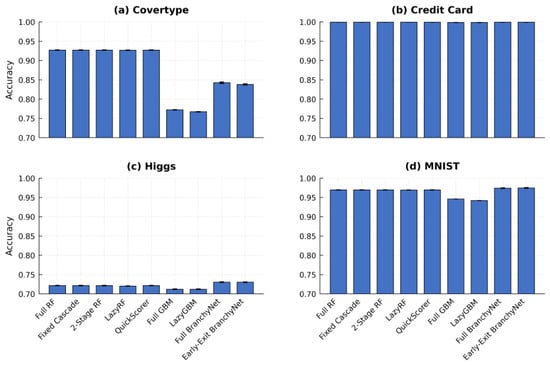
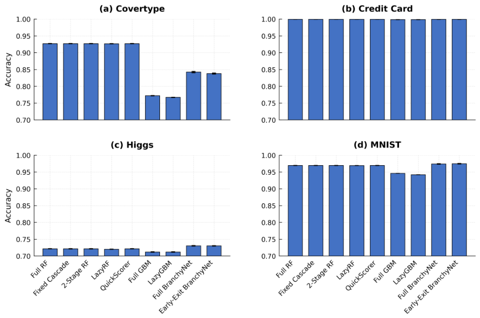
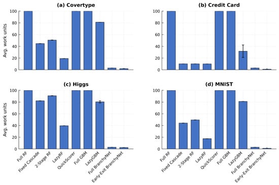
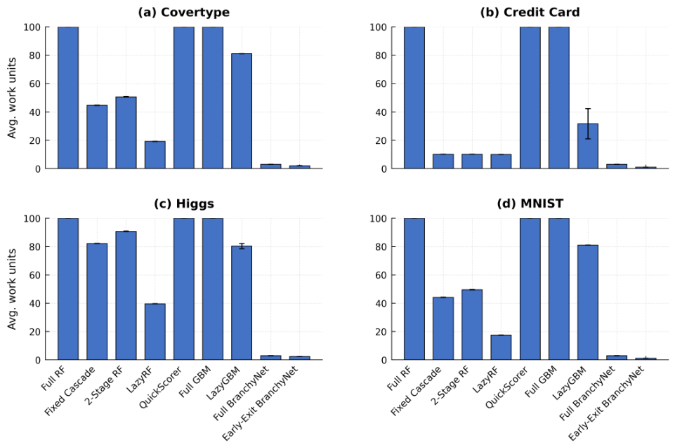
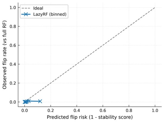
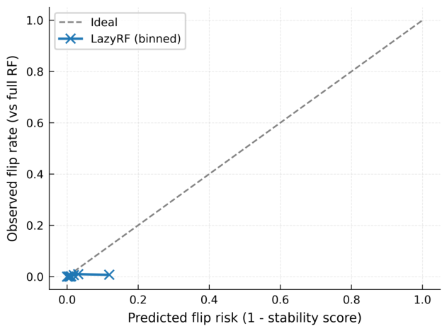

Disclaimer/Publisher’s Note: The statements, opinions and data contained in all publications are solely those of the individual author(s) and contributor(s) and not of MDPI and/or the editor(s). MDPI and/or the editor(s) disclaim responsibility for any injury to people or property resulting from any ideas, methods, instructions or products referred to in the content. |
© 2026 by the authors. Licensee MDPI, Basel, Switzerland. This article is an open access article distributed under the terms and conditions of the Creative Commons Attribution (CC BY) license.