Polynomial-Based Methods in Economic and Theoretical Statistics Courses: From Average Growth Speed Equations to Spatial Semiparametric Stochastic Frontier Estimation

Abstract

Statistics provides essential tools for transforming data into meaningful evidence for economic and scientific decision-making, while polynomial functions serve as a fundamental mathematical bridge that supports both economic and theoretical statistics. This paper aims to explore the applications to show how polynomial ideas support statistical learning from elementary computation to advanced estimation. First, in economic statistics, we reformulate the cumulative method for calculating average growth speed as a polynomial root-finding problem. We prove sufficient conditions for the existence and uniqueness of the economically meaningful positive root, thereby providing a rigorous foundation for a textbook procedure that is usually introduced without formal justification. We also extend the result to more general polynomial structures in which some coefficients may be negative. Second, in theoretical statistics, we develop a profile maximum likelihood estimation strategy for the spatial autoregressive nonparametric stochastic frontier model, where the unknown frontier function is approximated through a p-order local polynomial procedure. We derive the concentrated likelihood, construct the corresponding estimators, and provide an implementable bandwidth-selection algorithm. Numerical experiments verify the theoretical conclusions for the cumulative method and examine the finite-sample performance of the proposed estimator. Overall, this paper links polynomial root-finding in economic statistics with local polynomial estimation in nonparametric statistics.

1. Introduction

Statistics as an important tool has been widely applied in various fields [1,2], such as economics, sociology, management science and computer science, among others. Statistics course is a fundamental course for cultivating talents in various fields, with distinct practical value and solid methodological significance [3,4].

From the perspective of economic statistics, statistical methods provide fundamental tools for describing, comparing, and interpreting economic phenomena. Standard textbooks in statistics and business statistics emphasize the role of descriptive measures, index numbers, time-series comparisons, and growth-rate calculations in summarizing macroeconomic and firm-level changes [2,3,5,6,7]. In particular, the measurement of average growth rates is widely used in economic analysis because it transforms multi-period changes into a single interpretable indicator, thereby facilitating comparisons across regions, industries, and time periods. Chinese statistics textbooks usually introduce both the geometric mean method and the cumulative equation method when discussing average development or growth rates, highlighting their practical relevance to national income accounting, industrial output analysis, and other economic applications [2,3,8]. International textbooks on business and economic statistics similarly emphasize the importance of statistical summaries, probability-based reasoning, and time-series indicators in supporting economic decision-making under uncertainty [1,4,9,10]. These studies and textbooks collectively show that economic statistics is not merely a collection of computational techniques, but also an empirical framework for transforming economic data into meaningful evidence.

From the perspective of theoretical statistics, the calculation and estimation of economic indicators rely on rigorous mathematical foundations, including probability theory, sampling distributions, estimation theory, and numerical solution methods. General statistics textbooks systematically develop these foundations by linking descriptive statistics with inferential procedures, thereby providing the theoretical basis for parameter estimation, hypothesis testing, and model evaluation [1,2,3,4,5]. Econometric textbooks further extend these ideas by embedding statistical inference in regression models and stochastic economic systems, emphasizing consistency, efficiency, asymptotic properties, and the treatment of uncertainty in empirical analysis [11,12]. In the context of growth-rate estimation, the cumulative equation method can be viewed as a nonlinear equation-solving problem, in which the target growth rate is obtained by matching theoretical cumulative levels with observed cumulative values. This perspective connects applied economic statistics with numerical mathematics, since iterative algorithms such as the bisection method and Newton’s method are often used to obtain accurate solutions. Therefore, the relevant literature suggests that the study of economic statistical indicators should combine practical economic interpretation with formal statistical and numerical foundations, especially when the estimator is implicitly defined by a nonlinear equation.

This paper examines the application of polynomial functions in economic and theoretical statistics through two specific cases. First, in the economic statistics, the cumulative method for calculating the average growth speed is reformulated as a problem of finding the positive zero of a polynomial function. This reformulation transforms a commonly used computational rule into a mathematically justified problem. Unlike conventional textbook treatments, which often present the solution directly without proving its existence, uniqueness, or positivity, this paper establishes sufficient conditions under which the corresponding polynomial equation admits a unique positive root. It further shows that the standard average-growth-speed equation is nested as a special case of a more general polynomial structure.

Second, in the theoretical statistics course, the paper extends the role of polynomial functions to nonparametric stochastic frontier analysis by proposing a profile maximum likelihood estimation framework for a spatial autoregressive nonparametric stochastic frontier model, in which the unknown nonparametric component is estimated through a p-order local polynomial procedure. Based on this construction, the paper derives the concentrated likelihood function, obtains the profile estimators for the finite-dimensional parameters and the nonparametric frontier function, and further provides an implementable algorithm involving initial bandwidth selection and cross-validation-based bandwidth optimization. Therefore, the main contribution of the paper lies in connecting elementary statistical teaching and advanced econometric modeling through the common mathematical language of polynomial functions: on the one hand, it strengthens the theoretical foundation of a classical economic statistics topic; on the other hand, it demonstrates how higher-order polynomial approximation can support flexible nonparametric estimation in stochastic frontier analysis.

Although the average growth rate in economic statistics and the PMLE for spatial nonparametric stochastic frontier models differ substantially in application context and technical complexity, they are included in this paper under a unified pedagogical rationale. The former illustrates the explicit role of polynomial functions in a basic statistical computation problem, and the latter illustrates the implicit and advanced role of polynomial methodology in statistical estimation. This organization helps students understand polynomial functions as useful tools for statistical measurement, computation, and estimation.

Third, we conduct numerical experiments to examine the theoretical conclusions for the average growth speed in economic statistics and the finite-sample performance of the proposed profile maximum likelihood estimator. The results confirm that the polynomial equation generated by the cumulative method admits the same economically meaningful positive root under different numerical algorithms. They also show that Newton’s method converges rapidly when the initial value is close to the true root, but its performance becomes sensitive to the choice of the initial value when the starting point is far away. In contrast, the bisection method is generally slower but more stable. In addition, the simulation results for the spatial nonparametric stochastic frontier model indicate that the proposed PMLE performs better as the sample size increases.

The remainder of this paper is organized as follows. Section 2 makes a literature review. Section 3 provides the main results on the application of polynomial function in economic and theoretical statistics courses, respectively. Section 4 designs two kinds of numerical experiments to investigate the finite sample performance of iteration algorithms for solving the polynomial equation, and that of polynomial estimator. Section 5 further discusses the results and Section 6 concludes this paper. Additionally, Appendix A reports experimental results, and Appendix B gives the explanation for the lexicographic order.

2. Literature Review

One important application of polynomial functions in economic statistics is the calculation of the average growth rate using the cumulative method. Unlike the geometric method, which only matches the initial and terminal levels, the cumulative method determines the average development speed by requiring the cumulative theoretical levels to equal the cumulative observed levels Yuan et al. [2], Jia et al. [3], Zeng and Xiao [5]. This requirement naturally leads to a polynomial equation, in which the unknown average development speed is obtained as the positive zero of the polynomial. The mathematical validity of this procedure is closely related to the classical theory of polynomial zeros. The existence of a solution follows from the continuity of polynomial functions and the Intermediate Value theorem, as discussed in standard real analysis and numerical analysis texts Rudin [13], Apostol [14], Burden and Faires [15]. The uniqueness of the economically meaningful positive root can be established through monotonicity arguments when all cumulative theoretical coefficients are positive, or alternatively through Descartes’ rule of signs, which restricts the number of positive real roots Marden [16], Akritas [17]. Related root-location and root-counting results, including Sturm’s theorem and modern treatments of real-root isolation, further support the rigorous use of polynomial equations in statistical computation Collins and Akritas [18], Basu et al. [19]. Therefore, the cumulative method illustrates how polynomial functions provide a bridge between economic–statistical measurement and classical mathematical theory.

Local polynomial estimation in nonparametric stochastic frontier (SF) analysis has been developed in both classical and spatial SF models. For the classical model, building on the seminal stochastic frontier framework of Aigner et al. [20] and Meeusen and van den Broeck [21], early semiparametric extensions such as Fan et al. [22] allowed the production frontier to remain unspecified while preserving the composed-error structure. Later, Kumbhakar et al. [23] proposed a local maximum likelihood estimator for nonparametric SF models, providing a flexible way to estimate both the frontier and inefficiency components. Subsequent studies further improved identification, estimation, and inference in nonparametric and semiparametric SF models, including profile likelihood methods [24], categorical covariates [25], nonparametric least-squares estimation [26], endogenous regressors [27], and multiple-output settings [28]. To incorporate spatial dependence into SF analysis, Druska and Horrace [29] introduced spatial panel techniques into frontier estimation, while Schmidt et al. [30] emphasized spatially structured unobserved heterogeneity. More recent studies have developed spatial autoregressive SF models [31,32,33] and models allowing spatial dependence in both noise and inefficiency terms [34,35]. Closely related to this paper, Hou et al. [36] and Tran and Tsionas [37] extend spatial SF analysis to semiparametric and nonparametric settings.

3. The Application of Polynomial Functions in Statistics Courses

In this section, we mainly consider the application of the following polynomial function of order p ($p\in \mathbb{N}$) in teaching economic and theoretical statistics courses:

$$f\left(x\right)=a_p{x}^p+a_{p-1}{x}^{p-1}+\cdots +a_{1}x+a_0.$$

(1)

Here all polynomial coefficients are supposed to satisfy $a_i\in \mathbb{R}$ for $i=0,1,\cdots ,p$ and $a_p\ne 0$.

3.1. Economic Statistics Course: The Average Growth Speed

As a basic-level application, this subsection uses the average-growth-rate (AGR) problem in economic statistics to demonstrate how a routine statistical calculation can be rigorously interpreted through the existence and uniqueness of the positive root of a polynomial equation.

Suppose that ${\left\{y_t\right\}}_{t=1}^T$ is the sequence to explain some economic phenomenon with $y_t\ge 0$ for all t (Generally speaking, economic sequences are positive, such as GDP, national income, and national expenditure). The idea of a cumulative method is to guarantee that, under some AGR, say $x_G$, the sum of the theoretical level ($y_0{x}_G^t$, $y_0>0$ is the initial level) in each term is equal to that of practical level ($y_t$). Consequently, $x_G$ is the root of the equation

$$y_0(x+x^2+\cdots +x^T)={\displaystyle \sum _{t=1}^T}{y}_t.$$

(2)

Equivalently, $x_G$ is the zero point of the polynomial function $f\left(x\right)$ in (1), where $p=T$ and

$$a_T=a_{T-1}=\cdots =a_1=y_0>0\mathrm{and}{a}_0=-{\displaystyle \sum _{t=1}^T}{y}_t<0.$$

However, for the average-growth-rate application, existing statistics textbooks often present the cumulative method only as a numerical equation-solving procedure, without proving the existence, uniqueness, or positivity of the solution. Now, we establish the theorem for such existence and uniqueness, and prove this conclusion.

Theorem 1. 

Suppose that

$$a_i\ge 0\mathit{for}i=1,2,\cdots ,p\mathit{with}{a}_j>0\mathit{for}\mathit{some}j\in \{1,2\cdots ,p\},\mathit{and}{a}_0<0.$$

Then, the polynomial function of order p $f\left(x\right)$ in (1) has a unique positive zero point. Suppose further that ${\sum }_{i=0}^p{a}_i<0$, and then the unique positive zero point is greater than 1.

Proof. 

We first show the existence and uniqueness of the zero point to the polynomial function of order p $f\left(x\right)$ in (1). It is easy to verify that $f\left(x\right)$ is strictly increasing in $(0,+\infty )$. Notice that

$$f\left(0\right)=a_0<0\mathrm{and}\underset{x\to +\infty }{lim}f\left(x\right)=+\infty .$$

The local sign-preserving property implies that there exists a large enough number $x_1$ such that $f\left(x_1\right)>0$. Hence, $f\left(x\right)$ has a unique zero point in the interval $(0,x_1)$ because of Intermediate Value theorem [13].

Additionally, it follows from ${\sum }_{i=0}^p{a}_i<0$ that $f\left(1\right)={\sum }_{i=0}^p{a}_i<0$. Additionally, $\underset{x\to +\infty }{lim}f\left(x\right)=+\infty$ means that there exists a sufficiently large $N>0$ such that $f\left(N\right)>0$. Using Intermediate Value theorem again, the unique positive zero point is greater than 1. The proof is accomplished.    □

We can see from Theorem 1 that, if the constant is negative, and the other coefficients are nonnegative with at least one being positive, then the zero point exists and is unique. In fact, Theorem 1 provides a general result. In (2), except the constant, all the other coefficients are the same positive number, $y_0$. Theorem 1 just requires them to be nonnegative rather than the same positive number. Therefore, our Theorem 1 nests (2) as a special case.

Moreover, we find that when the constant in (1) is still negative and the coefficient of the highest-degree term is positive, that the other coefficients are negative also can derive the existence and the uniqueness of the zero point to the polynomial function of order p in (1). We establish the conclusion in the following Theorem 2.

Theorem 2. 

Suppose that

$$a_p>0,a_i\le 0\mathit{for}i=1,2,\cdots ,p-1\mathit{and}{a}_0<0.$$

Then, the polynomial function of order p $f\left(x\right)$ in (1) has a unique positive zero point. Suppose further that ${\sum }_{i=0}^p{a}_i<0$, and then the unique positive zero point is greater than 1.

Proof. 

This proof consists of three steps. The first step proves the existence of the positive zero point, the second step is to prove the uniqueness of such point, and the third step is to verify that the point is greater than 1 strictly.

In the first step, we show that there exists some positive number $x_{\ast }>0$ such that ${\left\{f^{\left(i\right)}\left(x\right)\right\}}_{i=1}^p$ is the sequence of positive polynomial functions as $x\in (x_{\ast },+\infty )$. By direct calculation, we can easily obtain that $f^{\left(p\right)}\left(x\right)=p!a_p>0$ holds strictly. This proves that the derivative function of $f\left(x\right)$ of order $p-1$ with respect to x,

$$f^{(p-1)}\left(x\right)={\displaystyle \frac{p!}{1}}{a}_{p}x+(p-1)!a_{p-1}$$

is monotonically increasing on the whole real line $(-\infty ,+\infty )$. No matter if $a_{p-1}<0$ or $a_{p-1}=0$, there exists some positive $x_1\in (0,+\infty )$ such that $f^{(p-1)}\left(x\right)>0$ if $x\in (x_1,+\infty )$ holds strictly. This proves that the derivative function of $f\left(x\right)$ of order $p-2$ with respect to x,

$$f^{(p-2)}\left(x\right)={\displaystyle \frac{p!}{2}}{a}_p{x}^2+{\displaystyle \frac{(p-1)!}{1}}{a}_{p-1}x+(p-2)!a_{p-2}$$

is monotonically increasing on the interval $(x_1,+\infty )\subset (0,+\infty )$. Given $f^{(p-2)}\left(x\right)$ is quadratic in the unknown x with the quadratic coefficient ${\displaystyle \frac{p!}{2}}{a}_p>0$, there exists some positive $x_2\in [x_1,+\infty )$ such that $f^{(p-2)}\left(x\right)>0$ if $x\in [x_2,+\infty )$ holds strictly. Similarly, there exists some positive sequence of numbers $x_{p-1}\ge x_{p-2}\ge \cdots \ge x_4\ge x_3$ such that

$$f^{(p-i)}\left(x\right)>0\mathrm{if}x>x_i,i=4,5,\cdots ,p-1.$$

The first step is accomplished by setting $x_{\ast }=x_{p-1}=max\{x_1,x_2,\cdots ,x_{p-1}\}>0$. Particularly, it follows that

$$f^{\left(1\right)}\left(x\right)=p{a}_p{x}^{p-1}+(p-1)a_{p-1}{x}^{p-2}+\cdots +a_{2}x+a_1>0$$

holds strictly if $x>x_{\ast }$. This tells us that the polynomial function of order p in (1), $f\left(x\right)$, is monotonically increasing on the interval $(x_{\ast },+\infty )\subset (0,+\infty )$. Working with the fact that $f\left(x\right)$ as a polynomial function is unbounded again, there exists some positive $x^{\ast }\in [x_{\ast },+\infty )$ such that $f\left(x\right)>0$ holds strictly if $x\in (x^{\ast },+\infty )$. Taking $f\left(0\right)=a_0<0$ together, $f\left(x\right)$ has at least one zero point in $(0,x^{\ast })$ because of Intermediate Value theorem.

In the second step, the uniqueness can be established by counter argument. Suppose that $0<x_1\ne x_2>0$ are two different positive zero points of $f\left(x\right)$ in (1). Define the mapping

$$T:{\mathbb{R}}^{+}\to {\mathbb{R}}^{+};x_1\mapsto T\left(x_1\right):={\left[{\displaystyle \frac{1}{a_p}}(-a_{p-1}{x}_1^{p-1}-\cdots -a_1{x}_1-a_0)\right]}^{{\displaystyle \frac{1}{p}}}.$$

Apparently, $T\left(x_1\right)$ is monotonically increasing on the interval $(0,+\infty )$, and we have

$$T\left(x_1\right)=x_1>0,T\left(x_2\right)=x_2>0.$$

If $x_1<x_2$, then there exists some $\eta <1$ such that $x_1=\eta x_2$. Consequently,

$$\begin{array}{cc}\hfill a_p{\left(\eta x_2\right)}^p& ={\eta }^p{a}_p{x}_2^p={\eta }^p(-a_{p-1}{x}_2^{p-1}-\cdots -a_1{x}_2-a_0)\hfill \\ & <{\eta }^p(-a_{p-1}{x}_2^{p-1}-\cdots -a_1{x}_2)-a_0.\hfill \end{array}$$

It follows that

$$T\left(\eta x_2\right)={\left[{\displaystyle \frac{1}{a_p}}({\eta }^p(-a_{p-1}{x}_2^{p-1}-\cdots -a_1{x}_2)-a_0)\right]}^{{\displaystyle \frac{1}{p}}}>\eta x_2.$$

(3)

In fact, $T\left(\eta x_2\right)=T\left(x_1\right)=x_1=\eta x_2$, which generates a contradiction to (3). So, $x_1\ge x_2$. Additionally, if we assume $x_1>x_2$, then we obtain $x_2\ge x_1$. In summary, $x_1=x_2$.

In the third step, the second conclusion follows from $f\left(1\right)<0$ similarly. The proof is accomplished.    □

Taking Theorems 1 and 2 together, we conclude that except the constant and the coefficient of the highest-degree term, the zero point to the polynomial function of order p (1) is still existent, no matter what the other coefficients are negative or nonnegative. We establish the conclusion in the following Corollary 1.

Corollary 1. 

Suppose that

$$a_p>0\mathit{and}{a}_0<0.$$

Then, the polynomial function of order p $f\left(x\right)$ in (1) has at least one positive zero point. Suppose further that ${\sum }_{i=0}^p{a}_i<0$, and then the positive zero point is greater than 1.

Proof. 

The proof is similar to that in Theorems 1 and 2.    □

Remark 1. 

Two things regarding Corollary 1 need pointing out. On the one hand, Corollary 1 shows that when the constant $a_0$ in (1) is still negative and the coefficient of the highest-degree term $a_p$ is positive, the existence of the zero point to the polynomial function of order p (1) still holds, no matter what the other coefficients $a_1,a_2\cdots ,a_{p-1}$ are negative or nonnegative. Although most economic variables are positive, some economic data or transformed indicators may take negative values. Therefore, this corollary extends the applicability of the previous results to a broader set of economic–statistical situations. On the other hand, under the condition in Corollary 1, we just guarantee the existence of such a zero point, and its uniqueness may not hold. For example, the cubic polynomial, $f\left(x\right)=(x-1)(x-2)(x-3)=x^3-6x^2+11x-6$, has three positive zero-points.

Theorems 1 and 2 and Corollary 1 are to connect a standard procedure in economic statistics with a rigorous mathematical justification. In many statistics textbooks, the cumulative method for calculating the average growth speed is introduced as an equation-solving rule, and the solution is usually obtained directly by numerical software. By reformulating this procedure as a polynomial root-finding problem, this subsection provides sufficient conditions under which the textbook procedure is mathematically well defined. In this sense, the result strengthens the theoretical foundation and classroom explanation of the cumulative method.

3.2. Theoretical Statistics Course: Nonparametric Stochastic Frontier Analysis

As an advanced-level application, this subsection extends polynomial ideas from explicit equation solving to local polynomial approximation, illustrating their role in estimating the nonparametric component of a spatial autoregressive stochastic frontier model. Typically, we propose the profile maximum likelihood estimation (PMLE) of the spatial autoregressive nonparametric stochastic frontier model in [37], where the nonparametric part is estimated by local polynomial regression. (Differently from our proposed PMLE, Ref. [37] considers the profile generalized method of moments (PGMM). Generally, provided that the stochastic terms have specific distributions, our PMLE is generally more efficient than PGMM when the distributional assumptions are correctly specified. Additionally, Ref. [37] assume $p=1$, and therefore our conclusion is more general.)

Start with the following model in [37]:

$$Y_n=\rho W_n{Y}_n+m\left(X_n\right)-U_n+V_n,V_n|X_n\sim N({\mathbf{0}}_n,{\sigma }_v^2{I}_n),U_n|X_n\sim N^{+}({\mathbf{0}}_n,{\sigma }_u^2{I}_n),$$

(4)

where n is the sample size, $Y_n\in {\mathbb{R}}^n$ is the observation on the explained variable, $X_n={[{\mathit{x}}_1,{\mathit{x}}_2,\cdots ,{\mathit{x}}_n]}^{\top }\in {\mathbb{R}}^{n\times k}$ is the observation on explanatory variables, $m\left(X_n\right)={[m\left({\mathit{x}}_1\right),m\left({\mathit{x}}_2\right),\cdots ,m\left({\mathit{x}}_n\right)]}^{\top }\in {\mathbb{R}}^n$ with $m:{\mathbb{R}}^k\to \mathbb{R}$ being some unknown fixed function, $\rho$ and $W_n\in {\mathbb{R}}^{n\times n}$ are successively the spatial lag parameter and spatial weight matrix with zero diagonals, $U_n={[u_1,u_2,\cdots ,u_n]}^{\top }$ capture technical inefficiencies in one-sided inefficiency terms, and $V_n={[v_1,v_2,\cdots ,v_n]}^{\top }$ capture statistic noise in both-sided disturbances. Denote $R_n\left(\rho \right)=I_n-\rho W_n$, and then the reduced-form of model (4) becomes

$$Y_n=R_n^{-1}\left(\rho \right)[m\left(X_n\right)-U_n+V_n],$$

(5)

provided that $R_n\left(\rho \right)$ is nonsingular. To estimate model (4) within the ML framework, we utilize the parameterization in [20] that ${\sigma }^2={\sigma }_v^2+{\sigma }_u^2$ and $\delta ={\sigma }_u/{\sigma }_v$ (Relative to the alternative in [38] that $\delta ={\sigma }_u^2/{\sigma }^2$). Denote $\theta ={[{\eta }^{\top },{\sigma }^2]}^{\top }$ with $\eta ={[\rho ,\delta ]}^{\top }$. Let

$${ϵ}_n\left(\theta \right)\triangleq {ϵ}_n(\theta ,m\left(X_n\right))=R_n\left(\rho \right)Y_n-m\left(X_n\right).$$

(6)

Then, Equation (2) [37] derives the log-likelihood function

$$\begin{array}{cc}\hfill L_n(\theta ,m\left(X_n\right))=& -{\displaystyle \frac{n}{2}}ln{\displaystyle \frac{\pi }{2}}-{\displaystyle \frac{n}{2}}ln\left({\sigma }^2\right)+ln\left|R_n\left(\rho \right)\right|-{\displaystyle \frac{1}{2{\sigma }^2}}{ϵ}_n^{\top }(\theta ,m\left(X_n\right)){ϵ}_n(\theta ,m\left(X_n\right))\hfill \\ \hfill & +{\displaystyle \sum _{i=1}^n}ln\Phi \left\{-{\displaystyle \frac{\delta }{\sigma }}{ϵ}_{ni}(\theta ,m\left(X_n\right))\right\}.\hfill \end{array}$$

(7)

Given [24]’s work, estimating $m(·)$ is a prerequisite since it is present in (4). The expectation of $R_n\left(\rho \right)Y_n$ conditional on $X_n$, however, is not equal to $m\left(X_n\right)$, i.e.,

$$\mathrm{E}\left[R_n\left(\rho \right)Y_n\right|X_n]=m\left(X_n\right)-\mu \left(\theta \right)\triangleq m^{†}(X_n,\theta ,m),$$

(8)

where $\mu \left(\theta \right)=\sigma {\left({\displaystyle \frac{2}{\pi }}{\displaystyle \frac{{\delta }^2}{1+{\delta }^2}}\right)}^{1/2}{\mathbf{1}}_n$, and $m^{†}(X_n,\theta ,m)={[m^{†}({\mathit{x}}_1,\theta ,m),\cdots ,m^{†}({\mathit{x}}_n,\theta ,m)]}^{\top }\in {\mathbb{R}}^n$. Apparently, existing nonparametric methods cannot be applied to estimate $m\left(\mathit{x}\right)$ directly. We now solve it by writing $m\left(X_n\right)=m^{†}(X_n,\theta ,m)+\mu$. Accordingly, we also have $m^{†}(X_n,\theta ,m)\triangleq m\left(X_n\right)-\mu \left(\theta \right)$, $\theta \in \Theta$, i.e.,

$$m\left(X_n\right)=m^{†}(X_n,\theta ,m)+\mu \left(\theta \right).$$

(9)

Even the parameter $\delta$ and ${\sigma }^2$ are contained on the right-hand side of (9), it is common to assume that $m\left(\mathit{x}\right)$ does not depend on $\theta$. This is general in classic (nonspatial) nonparametric analysis. In fact, this is in line with that in a conventional nonparametric setting. Such an assumption plays an important role in our strategy. This shall be explained later. Based on (9), we can rewrite

$${ϵ}_n(\theta ,m^{†}(X_n,\theta ,m)+\mu \left(\theta \right))=R_n\left(\rho \right)Y_n-m^{†}(X_n,\theta ,m)-\mu \left(\theta \right),$$

(6′)

and the log-likelihood function (7) becomes

$$\begin{array}{cc}& L_n\left(\theta ,m^{†}(X_n,\theta ,m)+\mu \left(\theta \right)\right)\hfill \\ \hfill =& -{\displaystyle \frac{n}{2}}ln{\displaystyle \frac{\pi }{2}}-{\displaystyle \frac{n}{2}}ln\left({\sigma }^2\right)+ln\left|R_n\left(\rho \right)\right|+{\displaystyle \sum _{i=1}^n}ln\Phi \left[-{\displaystyle \frac{\delta }{\sigma }}{ϵ}_{ni}(\theta ,m^{†}(X_n,\theta ,m)+\mu \left(\theta \right))\right]\hfill \\ & -{\displaystyle \frac{1}{2{\sigma }^2}}{ϵ}_n^{\top }(\theta ,m^{†}(X_n,\theta ,m)+\mu \left(\theta \right)){ϵ}_n(\theta ,m^{†}(X_n,\theta ,m)+\mu \left(\theta \right)),\hfill \end{array}$$

(7′)

where ${ϵ}_{ni}(·)$ is the $i^{\mathrm{th}}$ element of ${ϵ}_n(·)$. We see from (8) that $m^{†}(X_n,\theta ,m)$ depends on $\theta$ and m. Even so, (8) also tells us that $\mathrm{E}\left[R_n\left(\rho \right)Y_n\right|X_n]=m^{†}(X_n,\theta ,m)$. Thereby, for the dataset ${\{y_{ni},{\mathit{x}}_i\}}_{i=1}^n$, if $\rho$ is known, then $m^{†}(X_n,\theta ,m)$ can be estimated by the classic nonparametric technique. This indicates that the nonparametric estimation of $m^{†}(X_n,\theta ,m)$ only depends on $\rho$, say $m_{\eta }^{†}\left(\mathit{x}\right)$. This is similar to stage one of the estimation in [39].

To estimate model (4), we propose the three-step procedure for maximizing (7′). (i) Estimate $m^{†}(\mathit{x},\theta ,m)$ for fixed $\eta$, say $m_{\eta }^{†}\left(\mathit{x}\right)$. (ii) Estimate ${\sigma }^2$ for fixed $\eta$, say ${\sigma }_{\eta }^2\triangleq {\sigma }^2(\eta ,m_{\eta }^{†}\left(X_n\right)$, where $m^{†}(X_n,\theta ,m)$ has been replaced by $m_{\eta }^{†}\left(\mathit{x}\right)$. (iii) Replace $m^{†}(X_n,\theta ,m)$ and ${\sigma }^2$ successively by $m_{\eta }^{†}\left(X_n\right)$ and ${\sigma }_{\eta }^2$ into (7′), and obtain the concentrated log-likelihood function of $\eta$. By maximizing such a function, it produces the profile MLE ${\widehat{\theta }}_n$ and $m_{{\widehat{\rho }}_n}^{†}\left(\mathit{x}\right)$.

To estimate $m^{†}(\mathit{x},\theta ,m)$ for fixed $\rho$ in the first step, we use the named profile maximum likelihood estimation PMLE [40] method. The PMLE approach is applied to semiparametric stochastic frontier [22,24] and partially linear SAR models [39]. We will give the asymptotic analysis based on the local polynomial procedure [41,42]. For simplicity, we follow the notation in [43]. For any multi-dimensional index $\mathit{r}={[r_1,\dots ,r_k]}^{\top }\in {\mathbb{N}}_{\ast }^k$ and unknowns $\mathit{x}\in {\mathbb{R}}^k$, denote

$$\mathit{r}!={\displaystyle \prod _{i=1}^k}{r}_i!,\left|\mathit{r}\right|={\displaystyle \sum _{i=1}^k}{r}_i,\sum _{0\le \left|\mathit{r}\right|\le p}={\displaystyle \sum _{l=0}^p}{\displaystyle \sum _{r_1,\cdots ,r_k=0,\left|\mathit{r}\right|=1}^l},$$

${\mathit{x}}^{\mathit{r}}={\prod }_{i=1}^k{x}_i^{r_i}$, and $\left(D^{\mathit{r}}{m}^{†}\right)\left(\mathit{x}\right)={\displaystyle \frac{{\partial }^{\mathit{r}}{m}^{†}(\mathit{x},\theta ,m)}{\partial x_1^{r_1}\cdots \partial x_k^{r_k}}}$. Denote $N_l$ as the number of distinct $l^{\mathrm{th}}$ order derivatives of $m^{†}(\mathit{x},\theta ,m)$, and then $N_l=C_{q+l-1}^l$. For $\left|\mathit{r}\right|=0,1,\cdots ,p$, denote ${\beta }_{\mathit{r}}^{†}\left(\mathit{x}\right)$ as the scaled coefficient of ${\left({\mathit{x}}_i-\mathit{x}\right)}^{\mathit{r}}$ in the p-order Taylor expansion of $m_0^{†}\left({\mathit{x}}_i\right)$ around $\mathit{x}$, i.e.,

$${\beta }_{\mathit{r}}^{†}={\displaystyle \frac{h^{\left|\mathit{r}\right|}}{\mathit{r}!}}\left(D^{\mathit{r}}{m}^{†}\right)\left(\mathit{x}\right).$$

Further, according to the lexicographical order defined by (A3), for any $j\in \{1,2,\cdots ,N={\sum }_{l=0}^p{N}_l\}$, there exists the unique

$$\mathit{r}\equiv \mathit{r}\left(j\right)={[r_1\left(j\right),\cdots ,r_k\left(j\right)]}^{\top }\triangleq {[r_1,\cdots ,r_k]}^{\top }\in {\mathbb{N}}_{\ast }^k$$

such that $j={\sum }_{l=0}^{\overline{\mathit{r}}-1}{N}_l+g_{\overline{\mathit{r}}}^{†}\left(\mathit{r}\right)$, where $0\le g_{|\mathit{r}|}^{†}\left(\mathit{r}\right)<N_{|\mathit{r}|}$ and $\left|\mathit{r}\right|\in \{0,1,\cdots ,p\}$. In what follows of this article, $j\in \{1,2,\cdots ,N\}$ corresponds to $\mathit{r}\in \left\{\mathit{r}\ge {\mathbf{0}}_k:\left|\mathit{r}\right|\le p\right\}$ uniquely.

Let ${\beta }^{†}\left(\mathit{x}\right)=[{\beta }_0^{†}\left(\mathit{x}\right),{\beta }_1^{†\top }\left(\mathit{x}\right),\cdots ,{\beta }_p^{†\top }\left(\mathit{x}\right){]}^{\top }\in {\mathbb{R}}^N$ be a collection of all the parameters ${\beta }_{\mathit{r}}^{†}\left(\mathit{x}\right)$ with $\left|\mathit{r}\right|\le p$ in the lexicographical order (A3). Accordingly, given $\rho$, denote ${\beta }_{\rho }^{†}\left(\mathit{x}\right)=[{\beta }_{0,\rho }\left(\mathit{x}\right),{\beta }_{1,\rho }^{†\top }\left(\mathit{x}\right),\cdots ,{\beta }_{p,\rho }^{†\top }\left(\mathit{x}\right){]}^{\top }$ as the collection of the estimators ${\beta }_{\mathit{r},\theta }\left(\mathit{x}\right)$ for ${\beta }_{\mathit{r}}\left(\mathit{x}\right)$ with $\left|\mathit{r}\right|=l$ in the lexicographical order (A3). Set $K_h\left(\mathit{x}\right)=h^{-k}K(\mathit{x}/h)$, where $K(·)$ and h denote a kernel function on ${\mathbb{R}}^k$ and a bandwidth, respectively. For the dataset $\{Y_n,X_n\}$, given $\rho$, the p-order local polynomial of $S_{i,n}\left(\rho \right)Y_n$ on ${\mathit{x}}_i$ is

$${\beta }_{\rho }^{†}\left(\mathit{x}\right)=arg\underset{\beta }{min}{[R_n\left(\rho \right)Y_n-{\mathcal{X}}_n\left(\mathit{x}\right)H_n^{-1}\beta ]}^{\top }{\mathit{K}}_h\left(\mathit{x}\right)[R_n\left(\rho \right)Y_n-{\mathcal{X}}_n\left(\mathit{x}\right)H_n^{-1}\beta ],$$

(10)

where ${\mathit{K}}_h\left(\mathit{x}\right)\in {\mathbb{R}}^{n\times n}$ is the diagonal matrix with the ${(i,i)}^{\mathrm{th}}$ element being $K_h({\mathit{x}}_i-\mathit{x})$, and ${\mathcal{X}}_n\left(\mathit{x}\right)\in {\mathbb{R}}^{n\times N}$ with its ${(i,j)}^{\mathrm{th}}$ element being ${\mathcal{X}}_{n,ij}\left(\mathit{x}\right)={({\mathit{x}}_{ni}-\mathit{x})}^{\mathit{r}}$. Then, it yields from (10) that

$${\beta }_{\rho }^{†}\left(\mathit{x}\right)={\mathit{S}}_n\left(\mathit{x}\right)R_n\left(\rho \right)Y_n,$$

(11)

where the smoothing operator ${\mathit{S}}_n\left(\mathit{x}\right)={\left[H_n^{-1}{\mathcal{X}}_n^{\top }\left(\mathit{x}\right)K_n\left(\mathit{x}\right){\mathcal{X}}_n\left(\mathit{x}\right)H_n^{-1}\right]}^{-1}{H}_n^{-1}{\mathcal{X}}_n^{\top }\left(\mathit{x}\right)K_n\left(\mathit{x}\right)$. Particularly, given $\rho$, the estimator of $\mathrm{E}\left(R_n\left(\rho \right)Y_n\right|X_n)$ is given by

$$m_{\rho }^{†}\left(X_n\right)={[m_{\rho }^{†}\left({\mathit{x}}_1\right),m_{\rho }^{†}\left({\mathit{x}}_2\right),\cdots ,m_{\rho }^{†}\left({\mathit{x}}_n\right)]}^{\top }=S_n\left(X_n\right)R_n\left(\rho \right)Y_n,$$

(12)

where $S_n\left(X_n\right)\in {\mathbb{R}}^{n\times n}$ is defined by

$$S_n\left(X_n\right)=\left[\begin{array}{c}{\mathbf{e}}_{1,N}^{\top }{\mathit{S}}_n\left({\mathit{x}}_1\right)\\ {\mathbf{e}}_{1,N}^{\top }{\mathit{S}}_n\left({\mathit{x}}_2\right)\\ ⋮\\ {\mathbf{e}}_{1,N}^{\top }{\mathit{S}}_n\left({\mathit{x}}_n\right)\end{array}\right]$$

and ${\mathbf{e}}_{1,N}^{\top }=[1,0,\cdots ,0]\in {\mathbb{R}}^{1\times N}$.

In the second step, consider the estimation of ${\sigma }^2$ by maximizing the log-likelihood (7′). For fixed $\eta$ and $m^{†}(X_n,\theta ,m)$. It follows from $\partial ln{L}_n(·)/\partial \delta =\partial ln{L}_n(·)/\partial {\sigma }^2=0$ that

$${\displaystyle \frac{n}{2{\sigma }^2}}={\displaystyle \frac{1}{2{\sigma }^4}}{[R_n\left(\rho \right)Y_n-m^{†}(X_n,\theta ,m)-\mu \left(\theta \right)]}^{\top }[R_n\left(\rho \right)Y_n-m^{†}(X_n,\theta ,m)-\mu \left(\theta \right)].$$

(13)

Notice that $\mu \left(\theta \right)=\sigma {\left({\displaystyle \frac{2}{\pi }}{\displaystyle \frac{{\delta }^2}{1+{\delta }^2}}\right)}^{1/2}{\mathbf{1}}_n$. We see that, $\partial \mu \left(\theta \right)/\partial \theta$ is not equal to zero and it exists in the expression of $\partial ln{L}_n(·)/\partial \theta$. Even so, given $m\left(\mathit{x}\right)$ does not depend on $\theta$, it follows from (9) that

$${\displaystyle \frac{\partial [m^{†}(X_n,\theta ,m)+\mu \left(\theta \right)]}{\partial \theta }}={\displaystyle \frac{\partial m\left(X_n\right)}{\partial \theta }}={\mathbf{0}}_{3\times n}.$$

The useful pattern is also utilized in [22]. Estimated $m^{†}(X_n,\theta ,m)$ by $m_{\rho }^{†}\left(X_n\right)$ in (13), it yields a quadratic equation in the unknown ${\sigma }^2$ for given $\eta$. Accordingly, we obtain,

$${\widehat{\sigma }}_{\eta }^2={\left(1-{\displaystyle \frac{2}{\pi }}{\displaystyle \frac{{\delta }^2}{1+{\delta }^2}}\right)}^{-1}·{\displaystyle \frac{1}{n}}{Y}_n^{\top }{R}_n^{\top }\left(\rho \right){[I_n-S_n\left(X_n\right)]}^{\top }[I_n-S_n\left(X_n\right)]R_n\left(\rho \right)Y_n.$$

(14)

In the third step, replacing ${\sigma }^2$ by ${\widehat{\sigma }}_{\eta }^2$ and $m^{†}(X_n,\theta ,m)$ by $m_{\rho }^{†}\left(X_n\right)=S_n\left(X_n\right)R_n\left(\rho \right)Y_n$ in (7′), it produces the concentrated log-likelihood function of $\eta$,

$$L_n^c\left(\eta \right)=-{\displaystyle \frac{n}{2}}\left(ln{\displaystyle \frac{\pi }{2}}+1\right)-{\displaystyle \frac{n}{2}}ln{\widehat{\sigma }}_{\eta }^2+ln\left|R_n\left(\rho \right)\right|+{\displaystyle \sum _{i=1}^n}{l}_i\left(\eta \right),$$

(15)

where $l_i\left(\eta \right)=ln\Phi \left\{-\delta [{\widehat{\sigma }}_{\eta }^{-1}[{\mathbf{e}}_{i,n}^{\top }-{\mathbf{e}}_{i,N}^{\top }{\mathit{S}}_n\left({\mathit{x}}_i\right)]R_n\left(\rho \right)Y_n-{\left({\displaystyle \frac{2}{\pi }}{\displaystyle \frac{{\delta }^2}{1+{\delta }^2}}\right)}^{1/2}]\right\}$. Then, the MLE ${\widehat{\eta }}_n$ of $\eta$ maximizes the concentrated function (15), i.e.,

$${\widehat{\eta }}_n={[{\widehat{\rho }}_n,{\widehat{\delta }}_n]}^{\top }=arg\underset{\eta }{max}{L}_n^c\left(\eta \right).$$

(16)

Therefore, the plug-in estimator for ${\sigma }^2$ and the profile MLE for ${\beta }^{†}\left(\mathit{x}\right)$ are, respectively, ${\widehat{\sigma }}_n^2\triangleq {\widehat{\sigma }}_{{\widehat{\eta }}_n}^2$ and

$${\widehat{\beta }}_n^{†}\left(\mathit{x}\right)\triangleq {\beta }_{{\widehat{\rho }}_n}^{†}\left(\mathit{x}\right)={\mathit{S}}_n\left(\mathit{x}\right)R_n\left({\widehat{\rho }}_n\right)Y_n$$

(17)

Here ${\widehat{\sigma }}_{{\widehat{\eta }}_n}^2$ and ${\beta }_{{\widehat{\rho }}_n}^{†}\left(\mathit{x}\right)$ are defined successively in (14) and (11). A byproduct of the above procedure is

$${\widehat{m}}_n^{†}\left(X_n\right)=m_{{\widehat{\rho }}_n}^{†}\left(X_n\right)=S_n\left(X_n\right)R_n\left({\widehat{\rho }}_n\right)Y_n$$

(18)

according to (12). Particularly, the profile MLE ${\widehat{m}}_n^{†}\left(\mathit{x}\right)$ scaled partial derivatives up to order p. Additionally, $m\left(\mathit{x}\right)$ can be estimated by ${\widehat{m}}_n^{†}\left(\mathit{x}\right)+\mu \left({\widehat{\theta }}_n\right)$, where $\mu (·)$ is defined as in (8). The asymptotic properties of ${\widehat{\theta }}_n$ and ${\widehat{\beta }}_n^{†}\left(\mathit{x}\right)$ will be analyzed in subsequent sections.

Remark 2. 

Generally speaking, large sample properties of estimator in nonlinear spatial autoregressive models depend on the law of large numbers (LLN) and central limit theorem (CLT) in the spatial near-epoch dependence random field [44,45]. Under suitable regularity conditions, consistency and asymptotic normality of the PMLE estimator may be established following the LLN and CLT, although these theoretical properties are not formally proved in the present paper. Such regularity conditions should include the conventional nonparametric settings, and the properties of spatial NED random field and α-mixing sequences.

Actually, the above discussion is based on a given bandwidth h. However, it is difficult to specify the optimal bandwidth $h_{opt}$ in practice. Therefore, it is recommended a preliminary consistent estimator ${\tilde{\theta }}_n$ of $\theta$. Here, we suggest a two-step strategy for solving ${\widehat{\theta }}_n$ and ${\widehat{m}}_n^{†}\left(\mathit{x}\right)$ as follows (Algorithm 1).

Algorithm 1: PMLE for SAR-NP-SF model

Input: (i) the dataset ${\left\{({\mathit{x}}_i,y_i)\right\}}_{i=1}^N$; (ii) the order of polynomial function, p. Output: PMLE ${\widehat{\theta }}_n$ and ${\widehat{m}}_n^{†}\left(\mathit{x}\right)$ Step 1.1: Compute $h_{initial}={\left({\prod }_{i=1}^k{h}_{rot,i}\right)}^{1/k}$, where $h_{rot,i}=s_{x,i}·n^{-1/(k+4)}$ is chosen by a rule-of-thumb method with $s_{x,i}$ being the sample standard deviation of $\{x_{1,i},x_{2,i},\cdots ,x_{n,i}\}$; Step 1.2: Given $h_{initial}$, compute the estimate ${\tilde{\theta }}_n$ by (16) and (17) and ${\tilde{m}}_n^{†}\left(\mathit{x}\right)$ by (18); Step 2.1: Given ${\tilde{\theta }}_n$, conduct the least-squares cross-validation method to choose the optimal bandwidth by local polynomial regressing $S_n\left({\tilde{\rho }}_n\right)Y_n$ on $X_n$. Suppose that ${\widehat{m}}_{-i,n}^{†}\left({\mathit{x}}_i\right)$ is the leave-one-out estimator of $m^{†}({\mathit{x}}_i,\theta ,m)$, and obviously ${\widehat{m}}_{-i,n}^{†}\left({\mathit{x}}_i\right)$ must be the function of h. Specifically, $$h_{opt}=arg\underset{h}{min}C{V}_f\left(h\right),C{V}_f\left(h\right)=\sum _i{\left[R_{i,n}\left({\tilde{\rho }}_n\right)Y_n-{\widehat{m}}_{-i,n}^{†}\left({\mathit{x}}_i\right)\right]}^2,$$ (19) where $R_{i,n}(·)$ is the $i^{\mathrm{th}}$ row vector of $R_n(·)$; Step 2.2: Given $h_{opt}$, compute ${\tilde{\theta }}_n$ by (16) and (17) and ${\tilde{m}}_n^{†}\left(\mathit{x}\right)$ by (18) again.

4. Experiments

In this section, we conduct two kinds of numerical experiments to investigate the finite sample performance of iteration algorithms for solving the polynomial equations in Theorems 1 and 2 and Corollary 1, and that of PMLE for SAR-NP-SF model.

4.1. Growth Speed in Economic Statistics Course

For the following Examples 1 and 2, calculate the average growth rate using the cumulative method. We focus on Newton’s method and the bisection method because they represent two typical classes of root-finding algorithms commonly used in statistics and numerical analysis courses. Newton’s method is a derivative-based open method with fast local convergence but possible sensitivity to the initial value, whereas the bisection method is a bracketing method that is usually slower but more stable. Therefore, we hope to illustrate the trade-off between convergence speed and numerical robustness when solving the polynomial equation generated by the cumulative method.

Example 1. 

e.g., 7–11 [8] China’s GDP from 2015 to 2019 is shown in the second column of Table 1. Calculate the average growth rate of China’s gross domestic product from 2016 to 2019.

Table 1. China’s Gross Domestic Product from 2015 to 2019 (2015 constant prices).

Year	GDP
2015	688,858.2
2016	736,036.5
2017	787,170.4
2018	840,302.6
2019	891,646.1

Unit: hundred million yuan. Source: China Statistical Yearbook 2020.

According to the definition of cumulative method, the kernel point is to solve

$$\mathrm{688,858.2}(x+x^2+x^3+x^4)=\mathrm{736,036.5}+\mathrm{787,170.4}+\mathrm{840,302.6}+\mathrm{891,646.1},$$

which means that $a_4=a_3=a_2=a_1=\mathrm{688,858.2}$, and $a_0=-\mathrm{3,255,155.6}$.

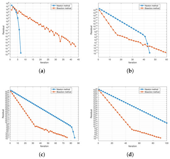
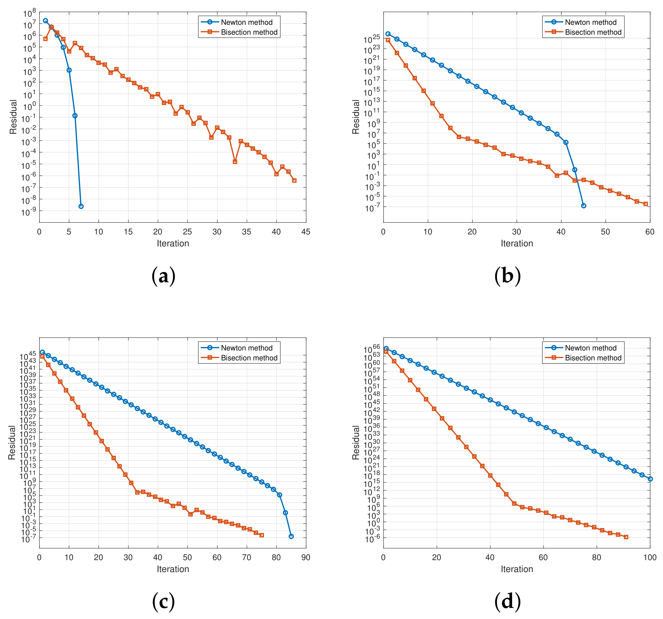
Table 2 reports the iteration steps spent by Newton iteration vs. Bisection method, and the convergent zero point. Figure 1 plots the comparison of residual descent between Newton’s method and bisection method.

Table 2. Comparison of Newton iteration vs. Bisection method for Example 1.

Initial Guess	Method	Solution	Iteration Steps
$x_0=2$	Newton iteration	1.0678	7
	Bisection iteration	1.0678	43
$x_0={10}^5$	Newton iteration	1.0678	44
	Bisection iteration	1.0678	59
$x_0={10}^{10}$	Newton iteration	1.0678	84
	Bisection iteration	1.0678	75
$x_0={10}^{15}$	Newton iteration	1.0678	101
	Bisection iteration	1.0678	92

Figure 1. Comparison of residual descent between Newton’s method and bisection method for Example 1. The initial iteration guess in (a), (b), (c) and (d) are $x_0=2$, $x_0={10}^5$, $x_0={10}^{10}$ and $x_0={10}^{15}$, respectively.

Example 2. 

ex. 52 [1] Hudson Marine has been an authorized dealer for C&D marine radios for the past seven years. The following Table 3 reports the number of radios sold each year. Calculate Hudson Marine’s annual average growth rate of the number of radios sold from 2 to 7.

Table 3. The number of radios sold each year from Hudson Marine.

Year	1	2	3	4	5	6	7
Number Sold	35	50	75	90	105	110	130

Similarly to Example 1, the kernel point is to solve the polynomial equation

$$35(x+x^2+x^3+x^4+x^5+x^6)=50+75+90+105+110+130,$$

which means that $a_6=a_5=a_4=a_3=a_2=a_1=35$ and $a_0=-560$.

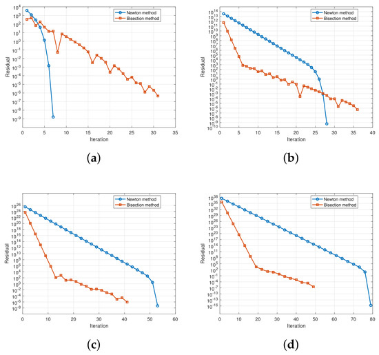
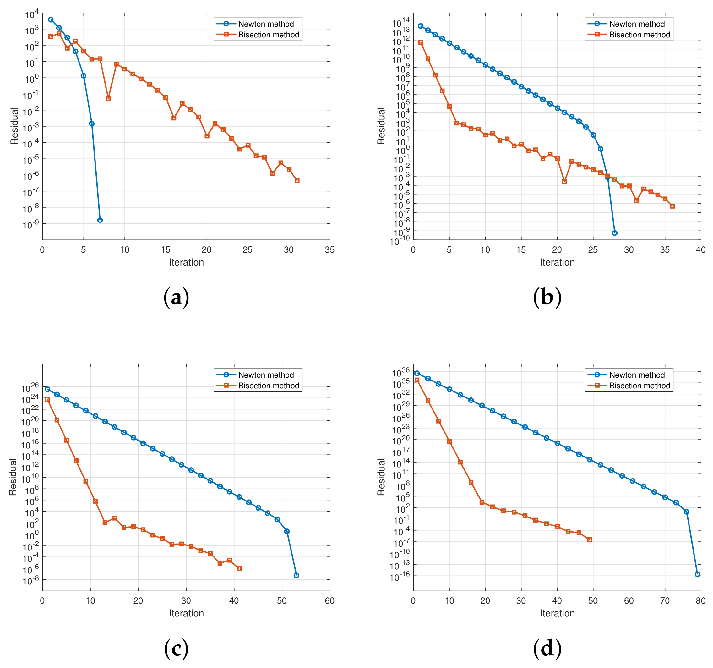
Table 4 reports the iteration steps spent by Newton iteration vs. Bisection method and the convergent zero point. Figure 2 plots the comparison of residual descent between Newton’s method and bisection method.

Table 4. Comparison of Newton iteration vs. Bisection method for Example 2.

Initial Guess	Method	Solution	Iteration Steps
$x_0=2$	Newton iteration	1.2890	7
	Bisection iteration	1.2890	31
$x_0={10}^2$	Newton iteration	1.2890	28
	Bisection iteration	1.2890	36
$x_0={10}^4$	Newton iteration	1.2890	53
	Bisection iteration	1.2890	41
$x_0={10}^6$	Newton iteration	1.2890	79
	Bisection iteration	1.2890	49

Figure 2. Comparison of residual descent between Newton’s method and bisection method for Example 2. The initial iteration guess in (a), (b), (c) and (d) are $x_0=2$, $x_0={10}^2$, $x_0={10}^4$ and $x_0={10}^6$, respectively.

The results in Table 2 and Table 4 show that both Newton’s method and the bisection method converge to the same positive root in the two examples, which is consistent with the theoretical conclusion that the polynomial equation generated by the cumulative method has a unique economically meaningful positive solution. However, the revised experiments provide a more nuanced comparison between the two algorithms. When the initial value is relatively close to the true root, Newton’s method converges much faster than the bisection method. For example, when ($x_0=2$), Newton’s method requires only 7 iterations in both examples, whereas the bisection method requires 43 and 31 iterations, respectively.

However, Newton’s method is more sensitive to the choice of the initial value. As the initial value moves farther away from the true root, its convergence speed decreases substantially. In Example 1, when ($x_0={10}^{10}$) and ($x_0={10}^{15}$), Newton’s method requires 84 and 101 iterations, respectively, which is slower than the bisection method. Similarly, in Example 2, when ($x_0={10}^4$) and ($x_0={10}^6$), Newton’s method requires 53 and 79 iterations, while the bisection method requires only 41 and 49 iterations. These results indicate that although Newton’s method has fast local convergence, its performance depends heavily on the initial value. By contrast, the bisection method is generally slower when the initial value is close to the root, but it is more stable and robust when the initial value is far away. Therefore, the numerical experiments highlight the practical importance of initial-value selection when applying iterative algorithms to solve the polynomial equation associated with the cumulative method.

4.2. SAR-NP-SF Models in Theoretical Statistics Course

In this section, we conduct Monte Carlo simulations to examine our proposed PMLEs’ finite sample performance in different scenarios, where various types of nonparametric settings are chosen.

We generate the data from the following data-generating processes (DGPs):

$$y_{ni}=\rho \sum _{j\ne i}{w}_{n,ij}{y}_{nj}+m\left(x_{ni}\right)-u_{ni}+v_{ni},i=1,\cdots ,n,$$

where the input variables $x_i$ are generated as i.i.d. $N(0,1)$ and the sample size varies among the set $\{5^2,7^2,{10}^2,{19}^2\}$. The spatial parameter is fixed $\rho =0.25$, and the spatial interaction among $y_{ni}$’s is the scenario based on the Queen criterion (P.8 [46]). Then, the matrix $W_n$ is row-normalized so that its row sums equal one, and its diagonal elements are set to zero. The function $m\left(x\right)$ is generated according to the following production function specifications in Fan et al. [22]:

• Model-1: $m\left(x\right)=1$;
• Model-2: $m\left(x\right)=1+x$;
• Model-3: $m\left(x\right)=1+ln\left(\right|1+x\left|\right)$;
• Model-4: $m\left(x\right)=1-{\displaystyle \frac{1}{1+\left|x\right|}}$.

For distributional parameters of the inefficiency $u_{ni}\sim N^{+}\left(0,{\sigma }_{uo}^2\right)$ and the two-sided error $v_{ni}\sim N\left(0,{\sigma }_{vo}^2\right)$, we use the same sets of values of the pair $({\sigma }_{vo}^2+{\sigma }_{uo}^2,{\sigma }_{uo}/{\sigma }_{vo})$ as listed in Table 2 of Aigner et al. [20] to facilitate comparison, that is, $\left\{\right(1.88,1.66),(1.63,1.24),$ (1.35, 0.83)} which corresponds to $({\sigma }_{vo}^2,{\sigma }_{uo}^2)\in \{(0.500,1.379),(0.339,0.901),(0.294,0.536)\}$. (Some of the literature also considers the same values in numerical experiments. See, e.g., Fan et al. [22], Parmeter and Racine [47], Martins-Filho and Yao [24], and Tran et al. [48].)

For the kernel function, we choose the Gaussian function. Given it is difficult to specify the optimal bandwidth sequence, we consider the optimal bandwidth $h_{opt}$ by conducting the least-squares cross-validation method in (19), which generates PMLE$\left(h_{opt}^{lscv}\right)$. Compute the bandwidth $h_{rot}$ by a rule-of-thumb method: $h_{rot}=s_x{n}^{-1/(q+4)}$, where $s_x$ is the sample standard deviation of $x_{ni}$’s and $q=1$. Here, we search for $h_{opt}$ in the iteration process with $h_{rot}$ as the initial iterative guess.

In the experiments, all results are based on 1000 replications. $W_n$ is fixed across all repetitions in each case, but the generated regressor $X_n$, $V_n$ and $U_n$ are randomly redrawn for each repetition.

Table A1, Table A2, Table A3 and Table A4 report some measures of central tendency and dispersions under different choices of the polynomial order p, sample size n, DGPs, and distributional parameter settings, mainly including the median absolute deviation, mean (MEAN), variance (VAR), mean square error (MSE) and the interdecile range (IDR), that is, the difference between the 90% quantile and 10% quantile of the empirical distribution.

Some patterns can be summarized from Table A1, Table A2, Table A3 and Table A4 as follows. Overall, the results show a clear improvement in estimation accuracy as the sample size increases, while the effect of increasing the polynomial order is relatively mild. First, holding the polynomial order fixed ($p=1$, $p=2$, and $p=3$), the estimators become more stable as n increases from 25 to 196. In almost all DGPs and parameter settings, the MAD, VAR, and IDR decline substantially with the sample size, indicating that the empirical distributions of the estimators become more concentrated around their central values. The reduction in dispersion is particularly evident when moving from $n=25$ to $n=100$, and remains visible, although more moderate, when n further increases to 196. The MSE also generally decreases with n, though the decline is less uniform than that of MAD, VAR, and IDR, especially for some cases involving ${\sigma }_v^2$. This suggests that larger samples mainly improve the precision and stability of the PMLEs.

Secondly, keeping the sample size constant and increasing p from 1 to 3 does not necessarily lead to an improvement in estimator performance. For each fixed n, the results under $p=1$, $p=2$, and $p=3$ are broadly comparable. In many cases, higher-order specifications slightly reduce MAD and IDR, especially under the nonlinear DGPs, suggesting that using a higher-order local polynomial may help capture nonlinear features of $m(·)$. However, the improvement is not uniform across all designs. In some cases, particularly when n is small, increasing p slightly raises the variance or MSE, reflecting the usual bias–variance trade-off associated with higher-order nonparametric estimation. Therefore, the gain from increasing p is much smaller than the gain from increasing n.

Taken together, the simulation evidence indicates that the proposed PMLEs exhibit satisfactory finite-sample behavior. The estimators become more precise and less dispersed as the sample size grows, regardless of whether $p=1$, $p=2$, or $p=3$. By contrast, the choice of p has only a secondary effect: higher-order polynomial specifications are generally competitive with lower-order ones and may perform slightly better in nonlinear designs, but they do not dominate uniformly. These findings suggest that sample size is the primary driver of finite-sample improvement, whereas the polynomial order mainly affects the bias–variance balance in specific DGPs.

5. Discussion

The practical value of this research lies in its ability to enhance the reliability of economic and scientific decision-making. In economic statistics, the cumulative method is vital for national income accounting and industrial output analysis. Our numerical experiments confirm that standard iterative algorithms, such as Newton’s method and the bisection method, are highly effective at obtaining accurate average growth rates from real-world data, such as China’s GDP. For theoretical applications, the proposed Algorithm 1 provides a robust tool for efficiency analysis in the presence of spatial dependence. The simulation results indicate that increasing sample size is the primary driver of improved estimation precision, offering a clear guideline for empirical researchers when designing spatial frontier studies.

In practice, for the average-growth-rate case, teachers may guide students from the textbook formula to the corresponding polynomial equation, then discuss the existence, uniqueness, and positivity of the solution, and finally use numerical algorithms to solve it. For the local-polynomial PMLE case, teachers may use it in advanced statistics or econometrics courses to show how polynomial approximation supports nonparametric estimation. Students can compare the roles of polynomial functions in basic computation and advanced estimation. Both make the pedagogical use of the cases clearer.

Despite the contributions, several areas for future exploration remain. First, while Corollary 1 guarantees the existence of a zero point under broader coefficient conditions, its uniqueness is not universally ensured, which may complicate interpretations in specific economic scenarios. Future research could focus on identifying additional constraints to guarantee uniqueness in these general cases. Second, the current nonparametric estimation performance in the SAR-NP-SF model is sensitive to bandwidth selection. Although we utilized a cross-validation strategy, further development of automated, data-driven bandwidth optimization could enhance the model’s scalability. Finally, future work could extend this polynomial framework to more complex empirical applications, such as analyzing asymmetric efficiency spillovers in global supply chains.

6. Conclusions

This paper highlights the role of polynomial functions in both economic and theoretical statistics. It first reformulates the cumulative method for calculating average growth rates as a polynomial root-finding problem and establishes formal conditions for the existence and uniqueness of its positive zero point, thereby strengthening the mathematical foundation of a commonly used teaching method. It then develops a profile maximum likelihood estimation procedure for a spatial autoregressive nonparametric stochastic frontier model, using local polynomial regression to estimate the unknown frontier function. Overall, the study connects elementary polynomial theory with modern statistical methodology and provides a unified perspective for applying polynomial functions in statistics. Future research may examine asymptotic properties and empirical applications.

References

- Anderson, D.R.; Sweeney, D.J.; Williams, T.A.; Camm, J.D.; Cochran, J.J. Statistics for Business and Economics, 13th ed.; Cengage Learning: Boston, MA, USA, 2017; pp. 863–864. [Google Scholar]
- Yuan, W.; Pang, H.; Jia, J.P.; Can, Y. Statistics, 5th ed.; Higher Education Press: Beijing, China, 2019. [Google Scholar]
- Jia, J.P.; He, X.Q.; Jin, Y.J. Statistics, 7th ed.; China Remin University Press: Beijing, China, 2018. [Google Scholar]
- Lind, D.A.; Marchal, W.G.; Wathen, S. Basic Statistics for Business & Economics, 9th ed.; McGraw-Hill Education: New York, NY, USA, 2019. [Google Scholar]
- Zeng, W.Y.; Xiao, H.Y. Introduction to Statistics; China Science Publishing & Media Ltd.: Beijing, China, 2023. [Google Scholar]
- Li, J.C. Statistics, 2nd ed.; Higher Education Press: Beijing, China, 2023. [Google Scholar]
- Fei, Y.; Shi, L. Statistics, 3rd ed.; Higher Education Press: Beijing, China, 2023. [Google Scholar]
- Zhang, H.M.; Fang, G.B. Statistics; Higher Education Press: Beijing, China, 2025; pp. 219–220. [Google Scholar]
- Newbold, P.; Carlson, W.L.; Thorne, B.M. Statistics for Business and Economics, 8th ed.; Pearson Education: Harlow, UK, 2013. [Google Scholar]
- Barrow, M. Statistics for Economics, Accounting and Business Studies, 7th ed.; Pearson Education: Harlow, UK, 2017. [Google Scholar]
- Greene, W.H. Econometric Analysis, 8th ed.; Pearson Education: Harlow, UK, 2020. [Google Scholar]
- Wooldridge, J.M. Introductory Econometrics: A Modern Approach, 7th ed.; Cengage Learning, Inc.: Boston, MA, USA, 2020. [Google Scholar]
- Rudin, W. Principles of Mathematical Analysis, 3rd ed.; McGraw-Hill, Inc.: New York, NY, USA, 1976. [Google Scholar]
- Apostol, T.M. Mathematical Analysis, 2nd ed.; Addison-Wesley Publishing Company: Reading, MA, USA, 1974. [Google Scholar]
- Burden, R.L.; Faires, J.D. Numerical Analysis, 9th ed.; Brooks/Cole, Cengage Learning: Boston, MA, USA, 2011. [Google Scholar]
- Marden, M. Geometry of Polynomials, 2nd ed.; American Mathematical Society: Providence, RI, USA, 1966. [Google Scholar]
- Akritas, A.G. Reflections on a Pair of Theorems by Budan and Fourier. Math. Mag. 1982, 55, 292–298. [Google Scholar] [CrossRef]
- Collins, G.E.; Akritas, A.G. Polynomial Real Root Isolation Using Descarte’s Rule of Signs. In Proceedings of the SYMSAC ’76: Third ACM Symposium on Symbolic and Algebraic Computation, New York, NY, USA, 10–12 August 1976; pp. 272–275. [Google Scholar] [CrossRef] [Scilit]
- Basu, S.; Pollack, R.; Roy, M.F. Algorithms and Computation in Mathematics. In Algorithms in Real Algebraic Geometry, 2nd ed.; Springer: Berlin/Heidelberg, Germany, 2006; Volume 10. [Google Scholar] [CrossRef] [Scilit]
- Aigner, D.; Lovell, C.A.K.; Schmidt, P. Formulation and Estimation of Stochastic Frontier Production Function Models. J. Econom. 1977, 6, 21–37. [Google Scholar] [CrossRef] [Scilit]
- Meeusen, W.; van den Broeck, J. Efficiency Estimation from Cobb-Douglas Production Functions with Composed Error. Int. Econ. Rev. 1977, 18, 435–444. [Google Scholar] [CrossRef] [Scilit]
- Fan, Y.; Li, Q.; Weersink, A. Semiparametric Estimation of Stochastic Production Frontier Models. J. Bus. Econ. Stat. 1996, 14, 460–468. [Google Scholar] [CrossRef] [Scilit]
- Kumbhakar, S.C.; Park, B.U.; Simar, L.; Tsionas, E.G. Nonparametric Stochastic Frontiers: A Local Maximum Likelihood Approach. J. Econom. 2007, 137, 1–27. [Google Scholar] [CrossRef] [Scilit]
- Martins-Filho, C.; Yao, F. Semiparametric Stochastic Frontier Estimation via Profile Likelihood. Econom. Rev. 2015, 34, 413–451. [Google Scholar]
- Park, B.U.; Simar, L.; Zelenyuk, V. Categorical Data in Local Maximum Likelihood: Theory and Applications to Productivity Analysis. J. Product. Anal. 2015, 43, 199–214. [Google Scholar]
- Simar, L.; Van Keilegom, I.; Zelenyuk, V. Nonparametric Least Squares Methods for Stochastic Frontier Models. J. Product. Anal. 2017, 47, 189–204. [Google Scholar]
- Prokhorov, A.; Tran, K.C.; Tsionas, M.G. Estimation of Semi- and Nonparametric Stochastic Frontier Models with Endogenous Regressors. Empir. Econ. 2021, 60, 3043–3068. [Google Scholar]
- Simar, L.; Wilson, P.W. Nonparametric Stochastic Frontier Models with Multiple Inputs and Outputs. J. Bus. Econ. Stat. 2023, 41, 1391–1403. [Google Scholar]
- Druska, V.; Horrace, W.C. Generalized Moments Estimation for Spatial Panel Data: Indonesian Rice Farming. Am. J. Agric. Econ. 2004, 86, 185–198. [Google Scholar] [CrossRef] [Scilit]
- Schmidt, A.M.; Moreira, A.R.B.; Helfand, S.M.; Fonseca, T.C.O. Spatial Stochastic Frontier Models: Accounting for Unobserved Local Determinants of Inefficiency. J. Product. Anal. 2009, 31, 101–112. [Google Scholar]
- Glass, A.J.; Kenjegalieva, K.; Sickles, R.C. A Spatial Autoregressive Stochastic Frontier Model for Panel Data with Asymmetric Efficiency Spillovers. J. Econom. 2016, 190, 289–300. [Google Scholar] [CrossRef] [Scilit]
- Kutlu, L. Estimating Efficiency in a Spatial Autoregressive Stochastic Frontier Model. Econ. Lett. 2018, 163, 155–157. [Google Scholar] [CrossRef] [Scilit]
- Tsukamoto, T. A Spatial Autoregressive Stochastic Frontier Model for Panel Data Incorporating A Model of Technical Inefficiency. JPN World Econ. 2019, 50, 66–77. [Google Scholar] [CrossRef] [Scilit]
- Orea, L.; Álvarez, I.C. A New Stochastic Frontier Model with Cross-Sectional Effects in Both Noise and Inefficiency Terms. J. Econom. 2019, 213, 556–577. [Google Scholar] [CrossRef] [Scilit]
- Kutlu, L.; Tran, K.C.; Tsionas, M.G. A Spatial Stochastic Frontier Model with Endogenous Frontier and Environmental Variables. Eur. J. Oper. Res. 2020, 286, 389–399. [Google Scholar] [CrossRef] [Scilit]
- Hou, Z.; Zhao, S.; Kumbhakar, S.C. The GMM Estimation of Semiparametric Spatial Stochastic Frontier Models. Eur. J. Oper. Res. 2023, 305, 1450–1464. [Google Scholar] [CrossRef] [Scilit]
- Tran, K.; Tsionas, M. Semiparametric Estimation of A Spatial Autoregressive Nonparametric Stochastic Frontier Model. J. Spat. Econom. 2023, 4, 7. [Google Scholar] [CrossRef] [Scilit]
- Battese, G.E.; Corra, G.S. Estimation of a Production Frontier Model: With Application to the Pastiral Zone of Eastern Australia. Aust. J. Agric. Resour. Econ. 1977, 21, 169–179. [Google Scholar] [CrossRef] [Scilit]
- Su, L.; Jin, S. Profile Quasi-Maximum Likelihood Estimation of Partially Linear Spatial Autoregressive Models. J. Econom. 2010, 157, 18–33. [Google Scholar] [CrossRef] [Scilit]
- Staniswalis, J.E. The Kernel Estimate of a Regression Function in Likelihood-Based Models. J. Am. Stat. Assoc. 1989, 84, 276–283. [Google Scholar] [CrossRef]
- Fan, J. Design-adaptive Nonparametric Regression. J. Am. Stat. Assoc. 1992, 87, 998–1004. [Google Scholar] [CrossRef]
- Fan, J.; Gijbels, I. Local Polynomial Modelling and Its Applications; Chapman and Hall: New York, NY, USA, 1996. [Google Scholar]
- Masry, E. Multivariate Regression Estimation: Local Polynomial Fitting for Time Series. Stoch. Process. Appl. 1996, 65, 81–101. [Google Scholar] [CrossRef] [Scilit]
- Jenish, N.; Prucha, I.R. Central Limit Theorems and Uniform Laws of Large Numbers for Arrays of Random Fields. J. Econom. 2009, 150, 86–98. [Google Scholar] [CrossRef] [Scilit] [PubMed]
- Jenish, N.; Prucha, I.R. On Spatial Processes and Asymptotic Inference under Near-Epoch Dependence. J. Econom. 2012, 170, 178–190. [Google Scholar] [CrossRef] [Scilit] [PubMed]
- Kelejian, H.; Piras, G. Spatial Econometrics; Academic Press: Cambridge, MA, USA, 2017. [Google Scholar]
- Parmeter, C.F.; Racine, J.S. Smooth Constrained Frontier Analysis; Springer: New York, NY, USA, 2013; pp. 463–488. [Google Scholar]
- Tran, K.C.; Tsionas, M.G.; Prokhorov, A.B. Semiparametric Estimation of Spatial Autoregressive Smooth-Coefficient Panel Stochastic Frontier Models. Eur. J. Oper. Res. 2023, 304, 1189–1199. [Google Scholar] [CrossRef] [Scilit]
Disclaimer/Publisher’s Note: The statements, opinions and data contained in all publications are solely those of the individual author(s) and contributor(s) and not of MDPI and/or the editor(s). MDPI and/or the editor(s) disclaim responsibility for any injury to people or property resulting from any ideas, methods, instructions or products referred to in the content. |
© 2026 by the authors. Licensee MDPI, Basel, Switzerland. This article is an open access article distributed under the terms and conditions of the Creative Commons Attribution (CC BY) license.