Bifurcation, Stability, and Nonlinear Vibration Analysis of a Harmonically Excited Duffing Oscillator Coupled with a Two-Degree-of-Freedom Nonlinear Energy Sink

Abstract

The study investigates the nonlinear dynamics of a harmonically excited Duffing oscillator coupled with an unforced two-degrees-of-freedom nonlinear energy sink. The external excitation is applied only to the primary oscillator; meanwhile, the NES response is induced through nonlinear internal coupling. The governing nonlinear ordinary differential equations are analyzed using the proposed non-perturbation approach, which does not rely on small-parameter assumptions or Taylor-series expansions. The formulation is used to obtain amplitude-dependent equivalent linear representations and analytical approximations of the coupled system. The analytical results are compared with direct numerical simulations, showing overall agreement with the full nonlinear model. The stability of the steady-state solutions is examined under variations of the main system parameters. The results indicate that the nonlinear coupling and stiffness parameters significantly affect the response amplitudes, stability characteristics, and overall dynamical behavior. Additional analyses using bifurcation diagrams, Lyapunov exponents, Poincaré maps, and basins of attraction reveal transitions between periodic, quasi-periodic, and chaotic regimes, as well as the presence of multi-stability and sensitivity to initial conditions. The proposed framework provides a useful analytical tool in studying the dynamics and stability of nonlinear oscillatory systems over a wide range of operating conditions.

1. Introduction

The suppression of unwanted vibrations in nonlinear mechanical systems remains an important topic in modern engineering due to the increasing use of lightweight, flexible, and high-performance structures. Effective vibration control is essential for limiting excessive oscillatory motion, reducing structural degradation, and improving dynamic performance. Conventional linear vibration absorbers, typically consisting of mass–spring–damper elements, often exhibit satisfactory performance only within relatively narrow frequency ranges. In contrast, NES has attracted considerable attention because of its ability to interact with a broad range of oscillatory responses through nonlinear coupling mechanisms. Consequently, NES configurations have been widely investigated in the context of vibration reduction and nonlinear dynamic analysis across various engineering applications [1,2,3,4,5,6,7].

Engineering structures such as bridges, aircraft, rotating machinery, MEMS/NEMS devices, offshore platforms, and civil infrastructures are frequently subjected to complex dynamic loads arising from seismic excitation, aerodynamic forces, traffic-induced vibrations, fluid–structure interaction, and machinery imbalance [8,9,10]. Under such operating conditions, damping mechanisms play a fundamental role in determining the stability and long-term dynamic performance of these systems. Energy dissipation may arise from viscous fluid interactions, internal material hysteresis, dry friction, or nonlinear interface effects between structural components [11,12,13,14,15,16]. Consequently, simplified damping models, including viscous, hysteretic, and Coulomb representations, are widely employed in analytical and NS of nonlinear vibrating systems. Among nonlinear oscillators, the Duffing oscillator has received considerable attention because of its ability to exhibit amplitude-dependent stiffness effects and a wide range of nonlinear dynamical responses, including multi-stability, bifurcations, and chaotic oscillations [17]. Such characteristics make Duffing-type systems a suitable framework for investigating nonlinear interactions and vibration-mitigation mechanisms in coupled oscillator configurations.

To analyze nonlinear oscillatory systems, HFF has emerged as an efficient analytical framework for establishing amplitude–frequency relationships in nonlinear oscillators [18,19,20,21,22,23,24,25,26]. Through suitable trial functions and weighted residual procedures, HFF has been successfully applied to a variety of nonlinear vibration problems. Complementary to HFF, the NPA has recently attracted attention as an alternative analytical tool for nonlinear and non-conservative oscillators without relying explicitly on asymptotic expansions or small perturbation parameters [27,28,29,30]. Within its range of applicability, the NPA provides equivalent representations that facilitate the analytical characterization of oscillatory responses and stability properties. When combined with direct NSs, the resulting framework enables a comprehensive investigation of transient behavior, steady-state responses, bifurcation scenarios, and complex nonlinear dynamics.

Although the governing equations considered in the present study are mathematically related to those of previously reported coupled oscillator–NES system, the system configuration differs from that of conventional coupled Duffing oscillators. In the present model, only the primary oscillator is externally excited, while the NES remains unforced and interacts through nonlinear coupling terms. This leads to a different interaction structure compared with fully forced coupled oscillator systems, which is considered in the present analysis. In contrast to perturbation-based formulations that rely on assumed harmonic representations and small-parameter assumptions, the present study employs NPA directly to the governing nonlinear ODEs to construct equivalent representations. This allows a unified treatment of both transient and steady-state behaviors within the same analytical framework.

Table 1 summarizes classical analytical approaches for nonlinear oscillatory systems alongside the proposed NPA in terms of their main assumptions and applicability. The classical methods typically rely on perturbation assumptions, harmonic truncation, or steady-state formulations, whereas the proposed NPA is formulated directly from the governing equations without small-parameter assumptions or asymptotic expansions, providing an equivalent amplitude-dependent representation within the weak-to-moderate nonlinear regime considered in this study. The purpose of this comparison is purely to clarify the formulation context of the proposed method.

Table 1. Comparison between the proposed NPA and classical analytical methods for nonlinear oscillatory systems.

Method	Main Assumption	Treatment of Nonlinearity/Forcing	Stability Treatment	Applicability/Complexity
MTSM	Small parameter assumption	Asymptotic/Taylor expansion	Indirect via modulation equations	Weak nonlinearity; moderate complexity
Averaging	Slow variation assumption	Period averaging	Approximate average system	Weak nonlinearity; low–moderate complexity
HBM	Periodic response assumption	Harmonic truncation	Algebraic steady-state system	Weak–moderate nonlinearity; moderate complexity
MCXA	Moderate nonlinear assumption	Complex harmonic expansion/steady-state formulation	Semi-direct (steady-state only)	Moderate regime; limited to steady-state analysis
NPA	No perturbation parameter	Equivalent amplitude-dependent formulation without truncation	Direct from the equivalent system	Weak-to-moderate nonlinear regime (investigated range); moderate complexity

The present work focuses on the development and application of NPA-based analytical formulation to investigate the nonlinear response behavior of a harmonically excited coupled oscillator–NES system under varying parameter conditions. The accurate prediction of stability characteristics together with nonlinear response transitions remains an active and important topic in nonlinear dynamics, particularly for strongly coupled multi-degree-of-freedom systems. Motivated by these considerations, the present study proposes a unified analytical framework for the coupled system, aiming to capture its dominant nonlinear dynamics and stability behavior in a consistent and mathematically tractable form. The main contributions of this work are summarized as follows:

• Development of NPA for a harmonically excited Duffing oscillator coupled with a 2DOF nonlinear energy sink.
• Derivation of amplitude-dependent equivalent linear representations of the nonlinear coupled system without the use of small-parameter assumptions, asymptotic expansions, or perturbation techniques.
• Analytical and numerical investigation of the stability characteristics and transition boundaries of the coupled system.
• Comprehensive numerical study of the system’s transient and steady-state nonlinear responses under varying parameter regimes.
• Validation of the proposed analytical formulation through direct numerical simulations of the original nonlinear governing equations.
• Systematic parametric investigation of the influence of key physical parameters on the system’s stability and nonlinear response behavior.

2. Construction of the Mechanical Model

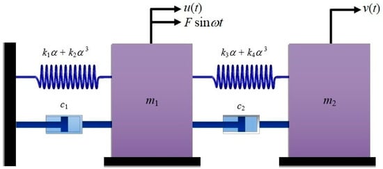
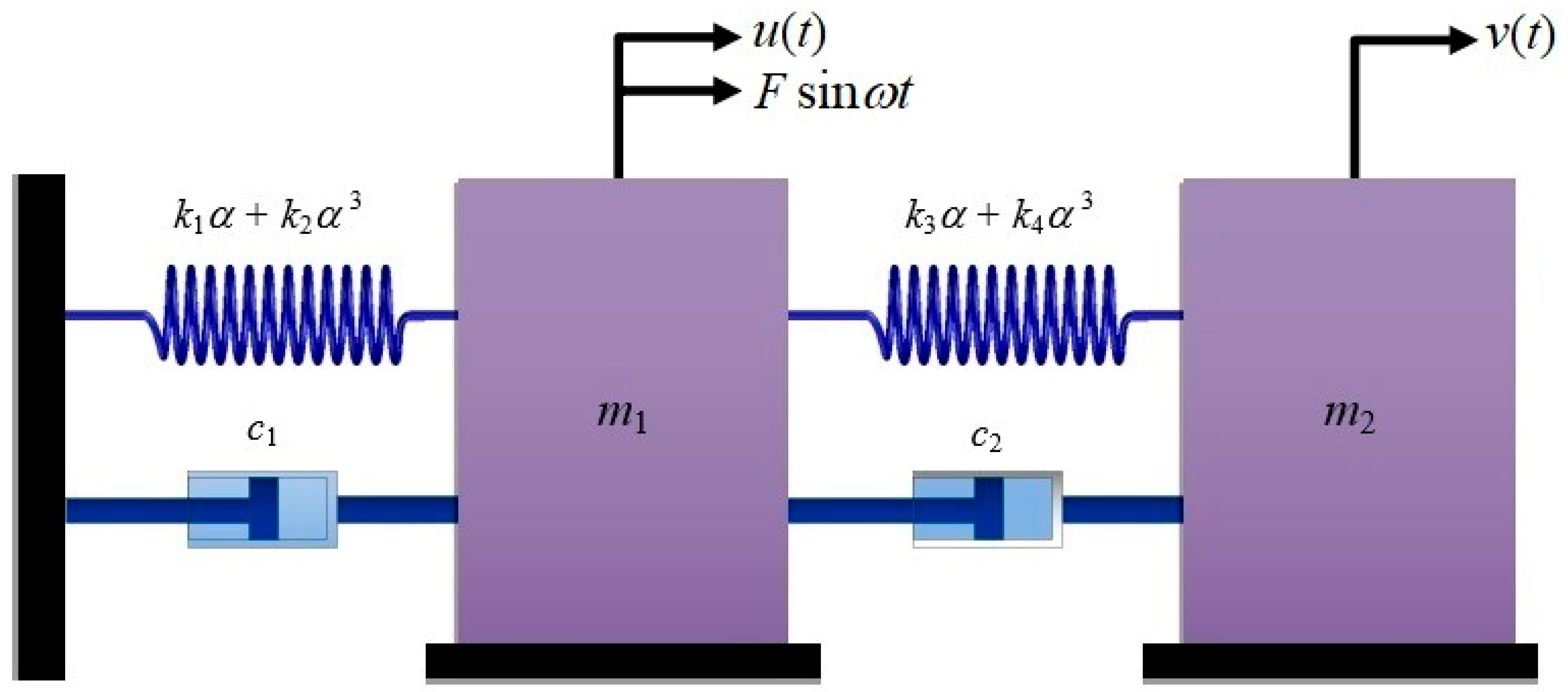
The present study considers a harmonically excited nonlinear oscillator coupled with a 2DOF-NES. Figure 1 demonstrates the mechanical configuration of the system. The primary oscillator consists of a mass $m_1$, a linear stiffness $k_1$, and a viscous damping coefficient $c_1$. The NES subsystem consists of a secondary mass $m_2$, coupled to the primary system through a linear stiffness $k_2$, a cubic nonlinear stiffness $k_4$, and a coupling damper $c_2$. The external excitation is given by a harmonic force of amplitude $F$ and frequency $\omega$, acting only on the primary oscillator.

Figure 1. Reflects a diagram of the nonlinear oscillator coupled to an ungrounded 2DOF of NES.

The present study considers a harmonically excited nonlinear oscillator coupled with a 2DOF-NES. The governing ODEs are given by the following coupled nonlinear system:

$$u^{″}+{\xi }_1{u}^{\prime }+u+{\beta }_1{u}^3+{\xi }_2(v^{\prime }-u^{\prime })+{\alpha }_2(v-u)+{\beta }_2{(v-u)}^3=f \sin \Omega t$$

(1)

and

$$v^{″}+r{\xi }_2(v^{\prime }-u^{\prime })+r{\alpha }_2(v-u)+r{\beta }_2{(v-u)}^3=0$$

(2)

where the primary oscillator is forced, while the NES is indirectly excited through nonlinear coupling terms.

For completeness and to ensure the self-contained nature of the manuscript, all dimensionless variables and parameters are summarized in Table 2. The symbol (′) denotes differentiation with respect to dimensionless time. The parameter $r=m_1/m_2$ represents the mass ratio between the NES and the primary system.

Table 2. Nomenclature and physical meaning of the dimensionless model parameters.

Symbol	Description	Physical Meaning
$u$	Primary displacement	Dimensionless displacement of the primary oscillator
$v$	NES displacement	Dimensionless displacement of the 2DOF of NES
${\xi }_1=c_1/m_1$	Primary damping	Viscous damping coefficient of the primary oscillator
${\xi }_2=c_2/m_2$	Coupling damping	Damping associated with energy exchange between the primary oscillator and the NES
${\alpha }_2=k_3/m_1$	Linear coupling stiffness	Dimensionless linear stiffness of the NES coupling
${\beta }_1=k_2/m_1$	Primary nonlinear stiffness	Cubic nonlinear stiffness of the primary oscillator
${\beta }_2=k_4/m_1$	NES nonlinear stiffness	Cubic nonlinear stiffness of NES
$f$	Forcing amplitude	Amplitude of external harmonic excitation
$\Omega$	Excitation frequency	Dimensionless forcing frequency

2.1. NPA Overview

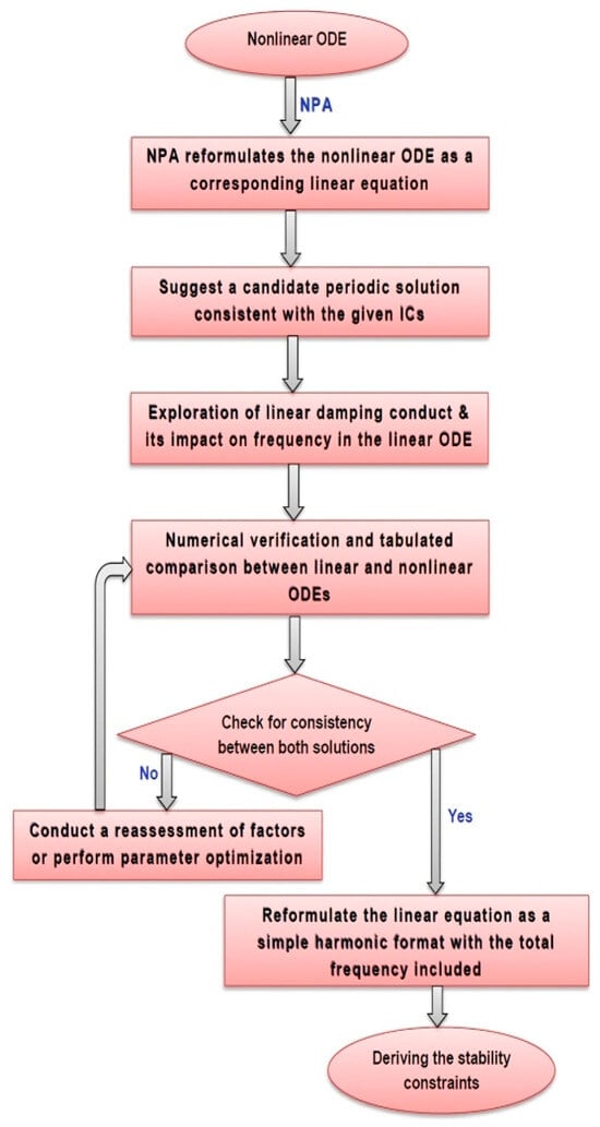
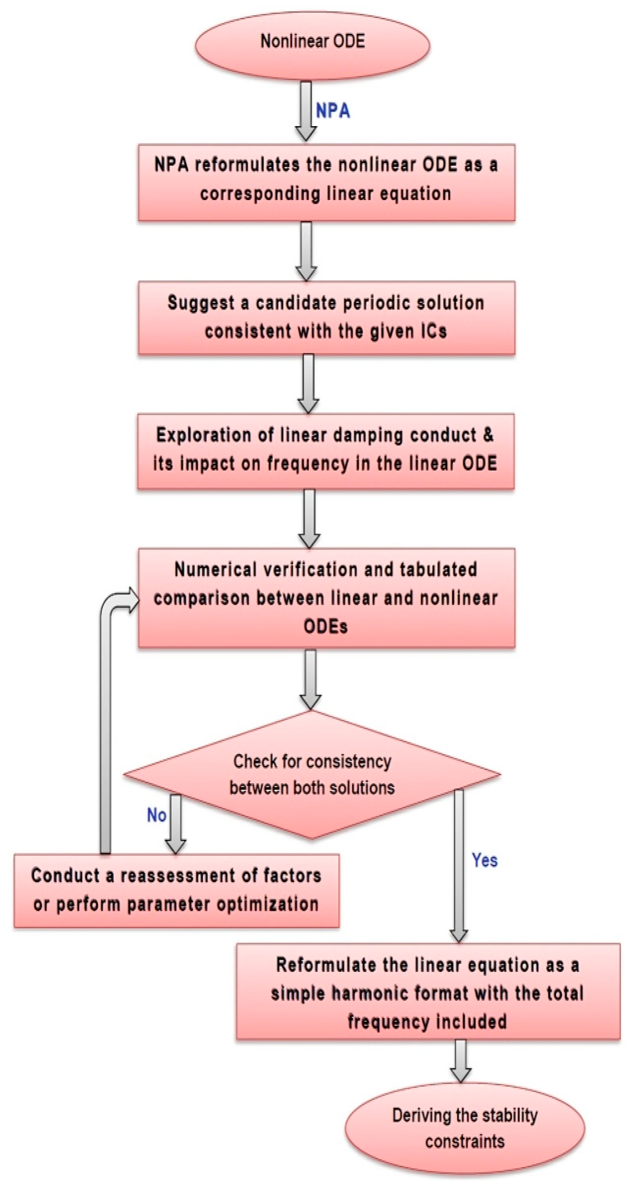
To ensure clarity, reproducibility, and methodological consistency, the NPA is presented through a structured step-by-step procedure, schematically illustrated in Figure 2. The method describes how the nonlinear ODEs governing the coupled 2DOF oscillator system are reformulated into equivalent amplitude-dependent linear representations, while retaining the dominant dynamical features of the original nonlinear system. The NPA begins with the selection of an appropriate single-harmonic trial function that represents the fundamental periodic behavior of the coupled system. This assumption provides the basis for transforming the original nonlinear governing ODEs into equivalent linear ones, where the effective damping and frequency parameters are determined through integral projections over a complete oscillation period. In contrast to perturbation-based methods or multi-harmonic expansions, the proposed formulation does not rely on small-parameter assumptions or truncated series expansions. This makes the approach applicable for analyzing weakly and moderately nonlinear regimes where the response is dominated by the fundamental harmonic component.

Figure 2. Shows a schematic representation of the proposed methodology.

2.2. Advantages of NPA

Compared with conventional analytical techniques, the NPA provides the key advantages of the NPA for analyzing nonlinear coupled oscillators, which can be summarized as follows:

• It preserves the complete set of original system parameters while providing an equivalent representation of the nonlinear dynamics.
• It yields a practically accurate analytical approximation without relying on exact closed-form solutions.
• It is applicable to weakly and moderately nonlinear systems without introducing small perturbation parameters or asymptotic expansions.
• It avoids Taylor-series expansion and the associated truncation of nonlinear terms.
• It is applicable to both damped and conservative nonlinear oscillator systems.
• It transforms the nonlinear governing equations into amplitude-dependent equivalent linear representations that are analytically tractable and readily implemented using standard computational platforms. In this study, MATLAB R2024a and Mathematica 12.00 were used, although the approach can also be implemented in other symbolic and numerical software packages. The analytical predictions show good agreement with direct numerical simulations of the original nonlinear model, supporting the accuracy and consistency of the proposed formulation for the cases investigated in this study.

2.3. Model Consistency and Limiting Cases

For further verification of the mathematical consistency of the proposed governing ODEs, several limiting cases are identified.

• In the absence of damping, forcing, and coupling nonlinearities ${\xi }_1={\xi }_2=f=0$, ${\alpha }_2=0$ and ${\beta }_2=0$ the system reduces to a Duffing oscillator representing the baseline nonlinear dynamics [31,32].
• Neglecting damping and external excitation $\left({\xi }_1={\xi }_2=f=0\right)$ reduces the system to a conservative two-degree-of-freedom nonlinear coupled oscillator [6].
• As the mass ratio approaches zero $\left(r\to 0\right)$, the inertia of the nonlinear attachment becomes negligible, and the governing equations reduce to a single forced nonlinear oscillator of Duffing-type.
• Setting ${\beta }_2=0$ removes the cubic nonlinear stiffness of the attachment, yielding a linearly coupled oscillator system [3].
• Setting ${\alpha }_2=0$ and ${\beta }_2=0$ eliminates all coupling nonlinearities, reducing the model to a single Duffing-type primary oscillator with cubic stiffness nonlinearity.
• Removing coupling and damping terms ${\alpha }_2={\xi }_2=0$ (and ${\beta }_2=0$ leads to an uncoupled forced Duffing oscillator as a limiting decoupled configuration.

These limiting cases confirm that the proposed formulation is consistent with several well-established models in nonlinear vibration theory, supporting the internal consistency of the governing ODEs. The system response is analyzed using both direct NSs and the equivalent analytical representation developed in the following section.

3. Theoretical Basis of the NPA

The NPA is developed for the coupled primary oscillator–2DOF-NES system. It reformulates the governing nonlinear ODEs into an equivalent amplitude-dependent representation that captures the dominant periodic response while enabling analytical treatment of the system dynamics.

The governing ODEs as specified in Equations (1) and (2) may be rewritten in equivalent forms as:

$$u^{″}+N_1(u^{\prime },v^{\prime })+N_2(u,v)=0,$$

(3)

and

$$v^{″}+D_1(u^{\prime },v^{\prime })+D_2(u,v)=0,$$

(4)

where the nonlinear damping and restoring contributions are decomposed into components associated with odd and secular terms, which are subsequently incorporated into the equivalent linear formulation through the NPA. These terms are expressed as:

$$\begin{gathered} N_1(u^{\prime },v^{\prime })={\xi }_1{u}^{\prime }+{\xi }_2(v^{\prime }-u^{\prime }), \\ {N}_2(u,v)=u+{\beta }_1{u}^3+{\alpha }_2(v-u)+{\beta }_2{(v-u)}^3-f\sin \Omega t{\displaystyle {\displaystyle \underset{0}{\overset{ع}{\int }}}du} \end{gathered}$$

(5)

$$D_1(u^{\prime },v^{\prime })=r{\xi }_2(v^{\prime }-u^{\prime }), \mathrm{and} D_2(u,v)=r{\alpha }_2(v-u)+r{\beta }_2{(v-u)}^3.$$

(6)

The formulation distinguishes between odd nonlinear terms contributing to the formulation distinguishes between odd nonlinear terms associated with equivalent damping and nonlinear restoring terms associated with equivalent stiffness. Following the masking technique of El-Dib [33,34,35], the quadratic nonlinear terms are incorporated into the equivalent transformed formulation without explicit expansion, while retaining their influence in the equivalent system. To construct the analytical approximation, single-harmonic trial functions are assumed for both oscillators as:

$$\tilde{x}=A\cos {\varpi }_{1}t,\mathrm{and} \tilde{y}=B\cos {\varpi }_{1}t,$$

(7)

and

$$\tilde{x}=A\cos {\varpi }_{2}t, \mathrm{and} \tilde{y}=B\cos {\varpi }_{2}t.$$

(8)

These trial solutions satisfy the ICs, which are given as follows:

$$u(0)=A, v(0)=B, u^{\prime }(0)=0, \mathrm{and} v^{\prime }(0)=0.$$

(9)

where $A, B$ being the initial amplitudes, whereas ${\varpi }_1$ and ${\varpi }_2$ are the total frequencies that define the assumed periodic response of each subsystem.

Substituting the assumed harmonic forms into the governing equations, the equivalent damping and stiffness coefficients are obtained through harmonic projection over one oscillation period of each subsystem. For the primary oscillator, $T_1=0\to 2\pi /{\varpi }_1$ and $T_2=0\to 2\pi /{\varpi }_2$ for the second one. This procedure is based on the orthogonality of trigonometric functions, ensuring consistent extraction of the fundamental harmonic contribution.

The admissible solution space is restricted to single-harmonic periodic functions, which represent the dominant response component of the system. No explicit optimization functional, weighting function, or least-squares minimization is introduced. The equivalent coefficients are obtained directly in closed form from projection integrals and are uniquely determined for given amplitudes and system parameters. This yields the equivalent linear system as [27,28,29,30].

$$x^{″}+{\chi }_{eqv1}{x}^{\prime }+{\Gamma }_{eqv1}^2 x=0,$$

(10)

and

$$y^{″}+{\chi }_{eqv2}{y}^{\prime }+{\Gamma }_{eqv2}^2 y=0.$$

(11)

with coefficients defined as:

$${\chi }_{eqv1}={\displaystyle {\displaystyle \underset{0}{\overset{2\pi /{\varpi }_1}{\int }}}{\tilde{x}}^{\prime }{N}_1({\tilde{x}}^{\prime }, {\tilde{y}}^{\prime })}dt/{\displaystyle {\displaystyle \underset{0}{\overset{2\pi /{\varpi }_1}{\int }}}{{\tilde{x}}^{\prime }}^2 dt}={\displaystyle \frac{1}{A}}\left(A\left( {\xi }_1- {\xi }_2\right)+B {\xi }_2\right),$$

(12)

$$\begin{array}{l}{\Gamma }_{eqv1}^2={\displaystyle {\displaystyle \underset{0}{\overset{2\pi /{\varpi }_1}{\int }}}\tilde{x} N_2(\tilde{x},\tilde{y})}dt/{\displaystyle {\displaystyle \underset{0}{\overset{2\pi /{\varpi }_1}{\int }}}{\tilde{x}}^2 dt}={\displaystyle \frac{1}{4A}}\left(3A^3{\beta }_1-3{\left(A-B\right)}^3{\beta }_2\right)\\ +{\displaystyle \frac{{\alpha }_2}{A}}\left( 2B-A\right)+\left(1/\pi \Omega \left({\Omega }^2-4{\varpi }_1^2\right)\right)\left(\left(1+2f\right)\pi {\Omega }^3-f{\Omega }^2{\varpi }_1-4\pi \left(1+f\right){\varpi }_1^2\Omega +2f{\varpi }_1^3,\right),\end{array}$$

(13)

$${\chi }_{eqv2}={\displaystyle {\displaystyle \underset{0}{\overset{2\pi /{\varpi }_2}{\int }}}{\tilde{y}}^{\prime } D_1({\tilde{x}}^{\prime }, {\tilde{y}}^{\prime })}dt/{\displaystyle {\displaystyle \underset{0}{\overset{2\pi /{\varpi }_2}{\int }}}{{\tilde{y}}^{\prime }}^2 dt}={\displaystyle \frac{r\left(B-A\right) {\xi }_2}{A}},$$

(14)

and

$${\Gamma }_{eqv2}^2={\displaystyle {\displaystyle \underset{0}{\overset{2\pi /{\varpi }_2}{\int }}}\tilde{y} D_2(\tilde{x}, \tilde{y})}dt/{\displaystyle {\displaystyle \underset{0}{\overset{2\pi /{\varpi }_2}{\int }}}{\tilde{y}}^2 dt}={\displaystyle \frac{r\left(B-A\right)}{4B}}\left(4{\alpha }_2+3{\beta }_2{\left(A-B\right)}^3\right).$$

(15)

Using standard coordinate transformations, one gets:

$$x(t)=\tilde{x} \mathrm{Exp}(-{\chi }_{eqv1} t/2),$$

(16)

and

$$y(t)=\tilde{y} \mathrm{Exp}(-{\chi }_{eqv2} t/2),$$

(17)

Substituting Equation (16) into Equation (10) and Equation (17) into Equation (11) yields the following reduced system:

$${\tilde{x}}^{″}+{\varpi }_1^2\tilde{x}=0,$$

(18)

and

$${\tilde{y}}^{″}+{\varpi }_2^2\tilde{y}=0.$$

(19)

Yielding

$${\varpi }_1^2={\Gamma }_{eqv1}^2-{\displaystyle \frac{1}{4}}{\chi }_{eqv1}^2,$$

(20)

and

$${\varpi }_2^2={\Gamma }_{eqv2}^2-{\displaystyle \frac{1}{4}}{\chi }_{eqv2}^2.$$

(21)

The stability boundaries are obtained from:

$${\varpi }_1^2>0, \mathrm{and} {\chi }_{eqv1}>0,$$

(22)

and

$${\varpi }_2^2>0, \mathrm{and} {\chi }_{eqv2}>0.$$

(23)

where ${\chi }_{eqv1,2}$ and ${\varpi }_{1,2}^2$ are the amplitude-dependent equivalent damping and overall frequency factors, respectively. The resulting stability conditions define transition curves separating stable and unstable regions in the amplitude–frequency parameter space.

The stability conditions derived from the equivalent linear system provide local analytical indicators associated with the equivalent NPA formulation. They are not intended to represent the global stability of the original nonlinear system. Accordingly, Floquet multipliers, stability tongues, bifurcation diagrams, Lyapunov exponent spectra, Poincaré sections, and basin of attraction analyses presented in this work are obtained independently through direct numerical integration of the original governing equations, Equations (1) and (2). These numerical analyses are used to investigate the global nonlinear dynamics, including multistability, quasi-periodicity, and chaotic responses, whereas the NPA is used to predict local stability trends of the equivalent system. The present formulation is applicable under the following assumptions:

• Weak-to-moderate nonlinear behavior, for which the adopted equivalent formulation remains valid.
• A system response dominated by the fundamental harmonic component.
• Initial oscillation amplitudes within the range $0<A,B\le 1$, for which the approximation provides reliable predictions in the present study.

Unlike equivalent linearization approaches based on residual minimization, the present NPA determines the equivalent coefficients directly through harmonic projection and cycle averaging, without introducing an explicit optimization functional or weighting function. Accordingly, the equivalent parameters are obtained through analytical projection onto the prescribed harmonic subspace rather than through an optimization procedure, yielding uniquely determined coefficients for a given set of amplitudes and system parameters.

Numerical Implementation Details

The governing equations are solved using the NDSolve function in Mathematica 12.00. with adaptive step-size integration. Simulations are performed over sufficiently long time intervals, and transient responses are removed before analysis. Lyapunov exponents are computed using the Benettin algorithm with Gram–Schmidt re-orthonormalization. Poincaré sections are constructed using stroboscopic sampling synchronized with excitation frequency. Bifurcation diagrams are obtained using parameter sweep continuation. MATLAB R2024a was used for post-processing and visualization.

4. Validation and Error Analysis of the Proposed NPA

To verify the accuracy of the proposed analytical formulation, a systematic validation is performed through numerical comparison and error quantification. The validation includes:

a.

Time-domain comparison between the two solutions.

b.

Quantitative error analysis to evaluate the deviation between the two solutions.

All simulations are carried out using adaptive time-stepping in NDSolve, with sufficiently high accuracy and precision settings to guarantee numerical convergence. Both models are solved under identical numerical conditions to ensure a fair and consistent comparison. The dimensionless parameters employed in the present simulations are selected within physically realistic and numerically stable ranges commonly used in nonlinear vibration studies.

4.1. Validation of the Primary Oscillator

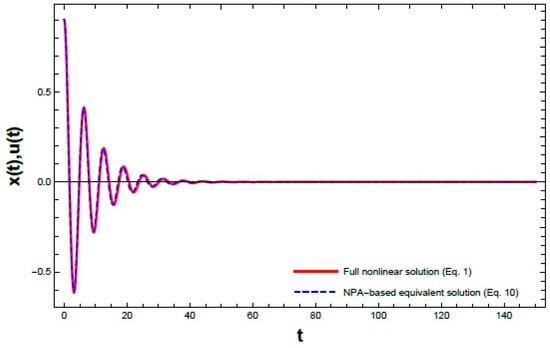
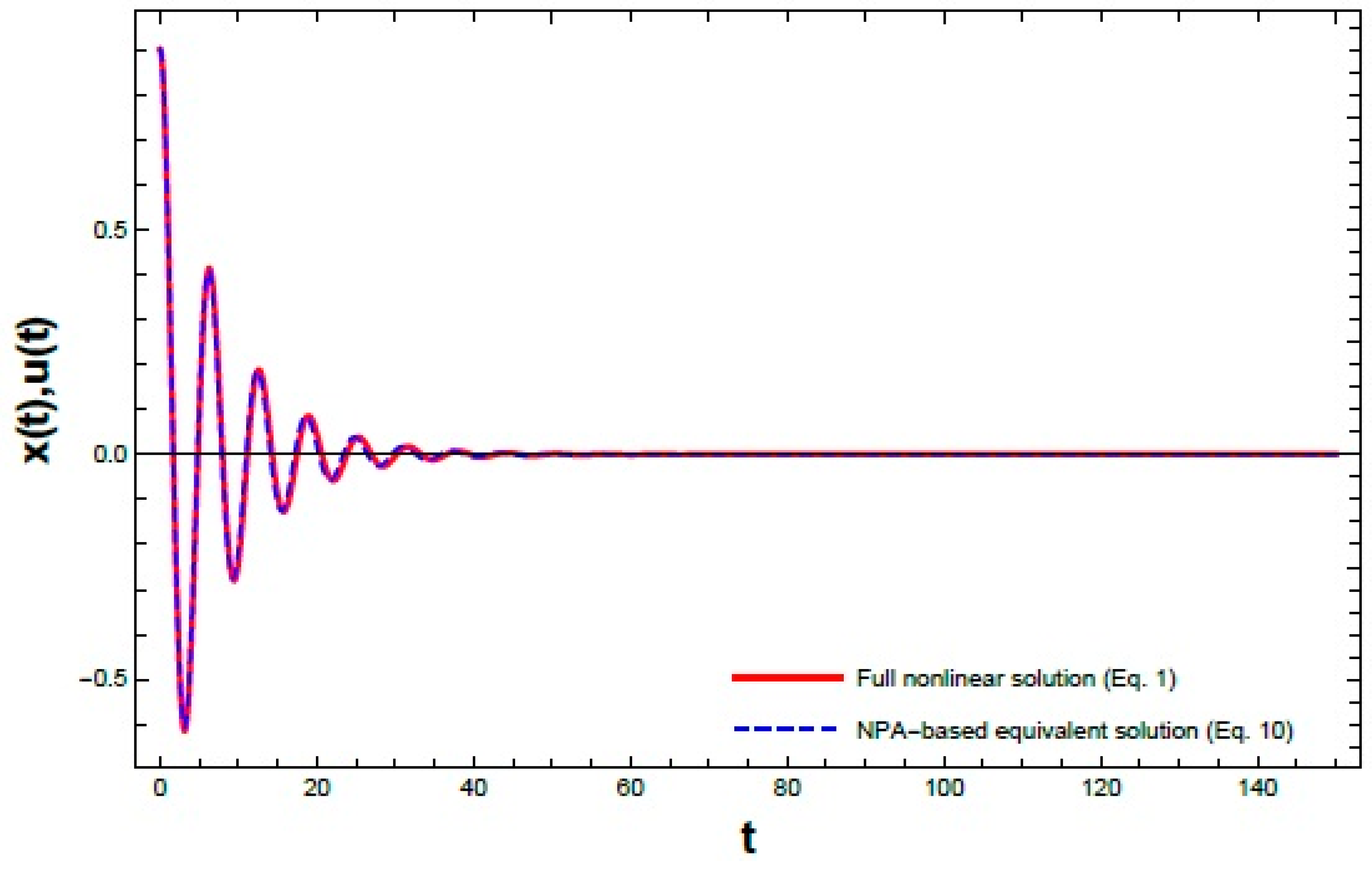
Figure 3 presents the displacement–time response obtained from NPA of Equation (10) formulation and the NS of Equation (1). The displacement histories are plotted on the same graph to examine the correspondence between both solutions in terms of amplitude and phase evolution. A close agreement is observed throughout the investigated interval $t\in \left[0, 150\right]$, including both transient and steady-state regions. This behavior indicates consistency between the two representations and supports the validity of the proposed NPA formulation within the considered parameter range (see Figure 3).

Figure 3. Shows comparison between the time responses of the primary oscillator obtained from the full nonlinear system as given in Equation (1) and the corresponding NPA equivalent model as shown in Equation (10) under identical ICs and parameter set: $A=0.9, B=0.12, r=0.07. {\xi }_1=0.3$, ${\xi }_2=0.07, f=0.01,\Omega =0.1$, ${\beta }_1=0.1, {\beta }_2=0.04$ and ${\alpha }_2=0.08$.

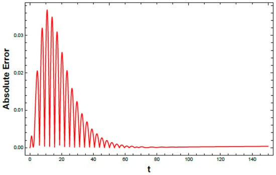
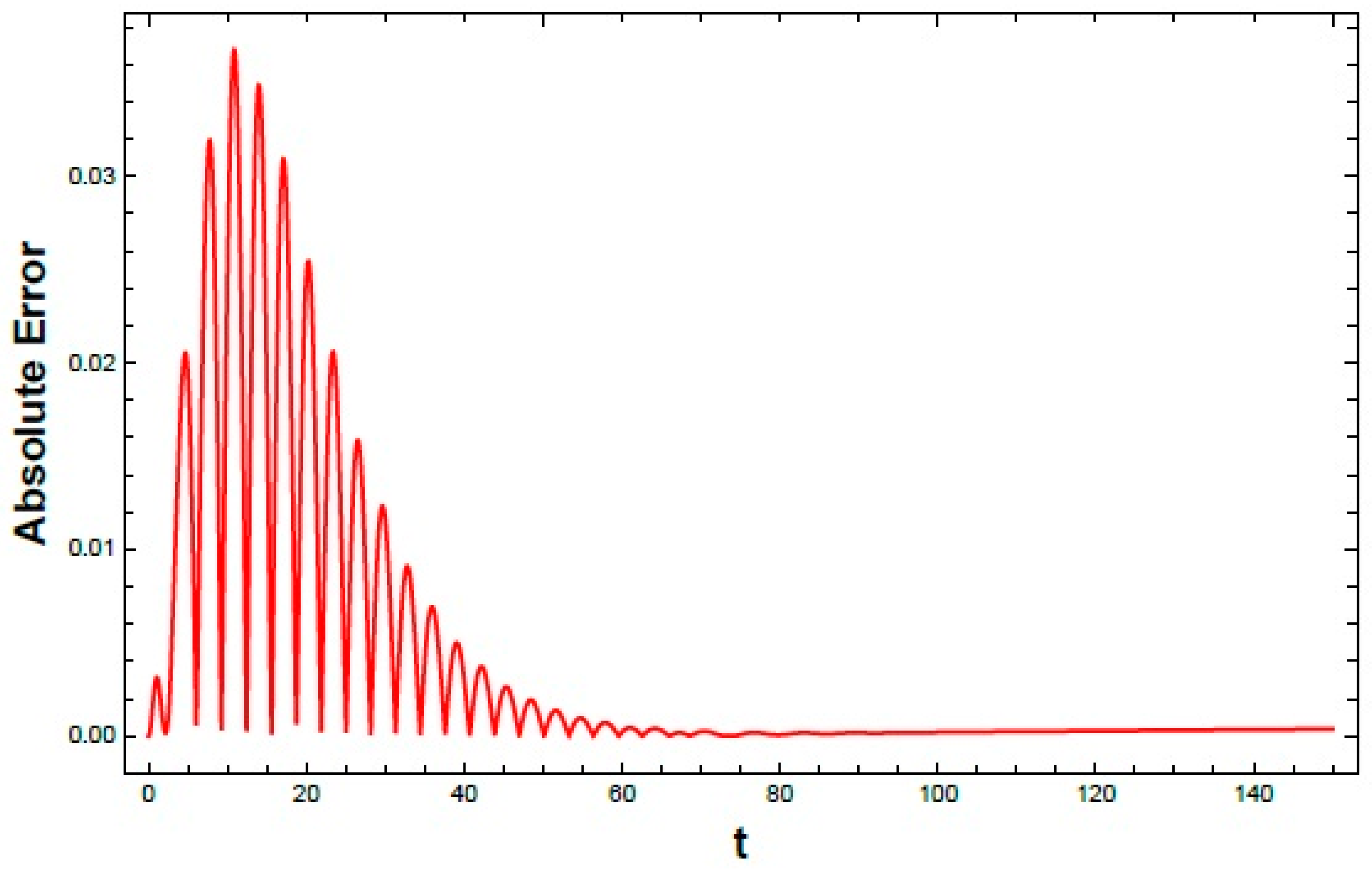
To further quantify the difference between the NPA and NS results, the Absolute error evolution is shown in Figure 4. The error remains small throughout the simulation interval $t\in \left[0, 150\right]$, indicating overall agreement between both solutions. A slight increase is observed in the initial transient stage due to nonlinear effects. As the response approaches steady state, the error becomes nearly bounded within a narrow oscillatory range, with no indication of divergence.

Figure 4. Shows the time evolution of the absolute errors between the NS and NPA solutions.

4.2. Validation of the Second Oscillator (NES)

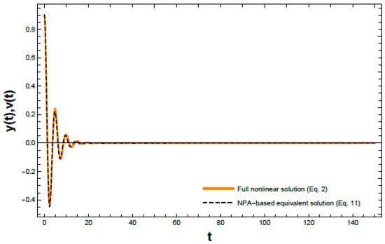
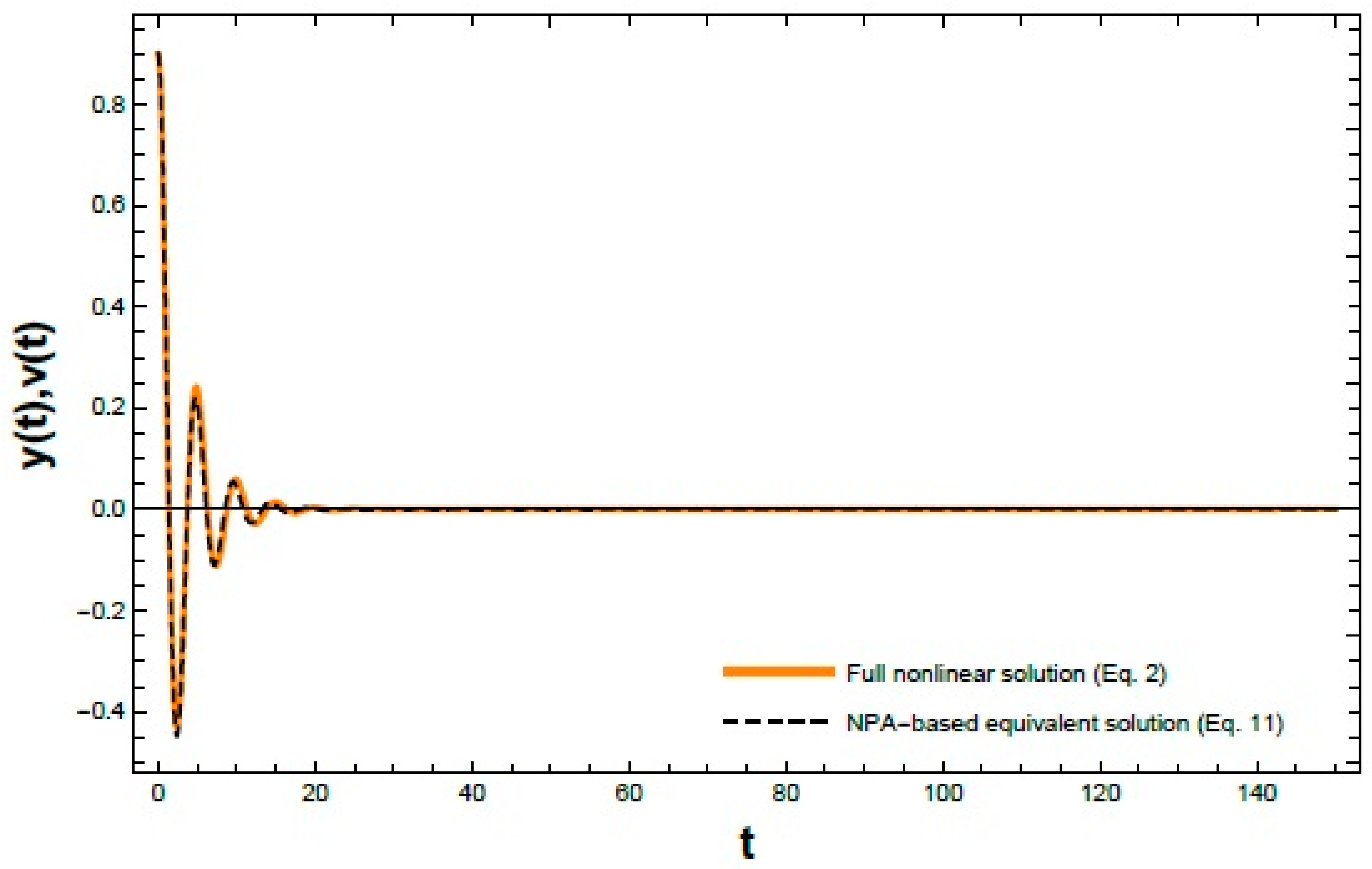
Figure 5 shows the displacement–time response obtained from both the NPA of Equation (11) formulation and the NS Equation (2). The displacement histories are plotted together to assess the agreement in amplitude and phase evolution. A close match is observed over the entire investigated interval $t\in \left[0, 150\right]$, including both transient and steady-state regimes. These results indicate good consistency between both representations and support the validity of the proposed NPA formulation.

Figure 5. Shows comparison between the time responses of the NES obtained from the full coupled nonlinear system (Equation (2)) and its corresponding NPA-based equivalent representation as given in Equation (11) under the same initial conditions and parameter values: $A=0.09, B=0.9, {\xi }_1=3.2$, ${\xi }_2=0.078, f=0.04,\Omega =0.08$, ${\beta }_1=0.1, {\beta }_2=0.7$ and ${\alpha }_2=0.2$.

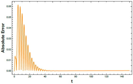
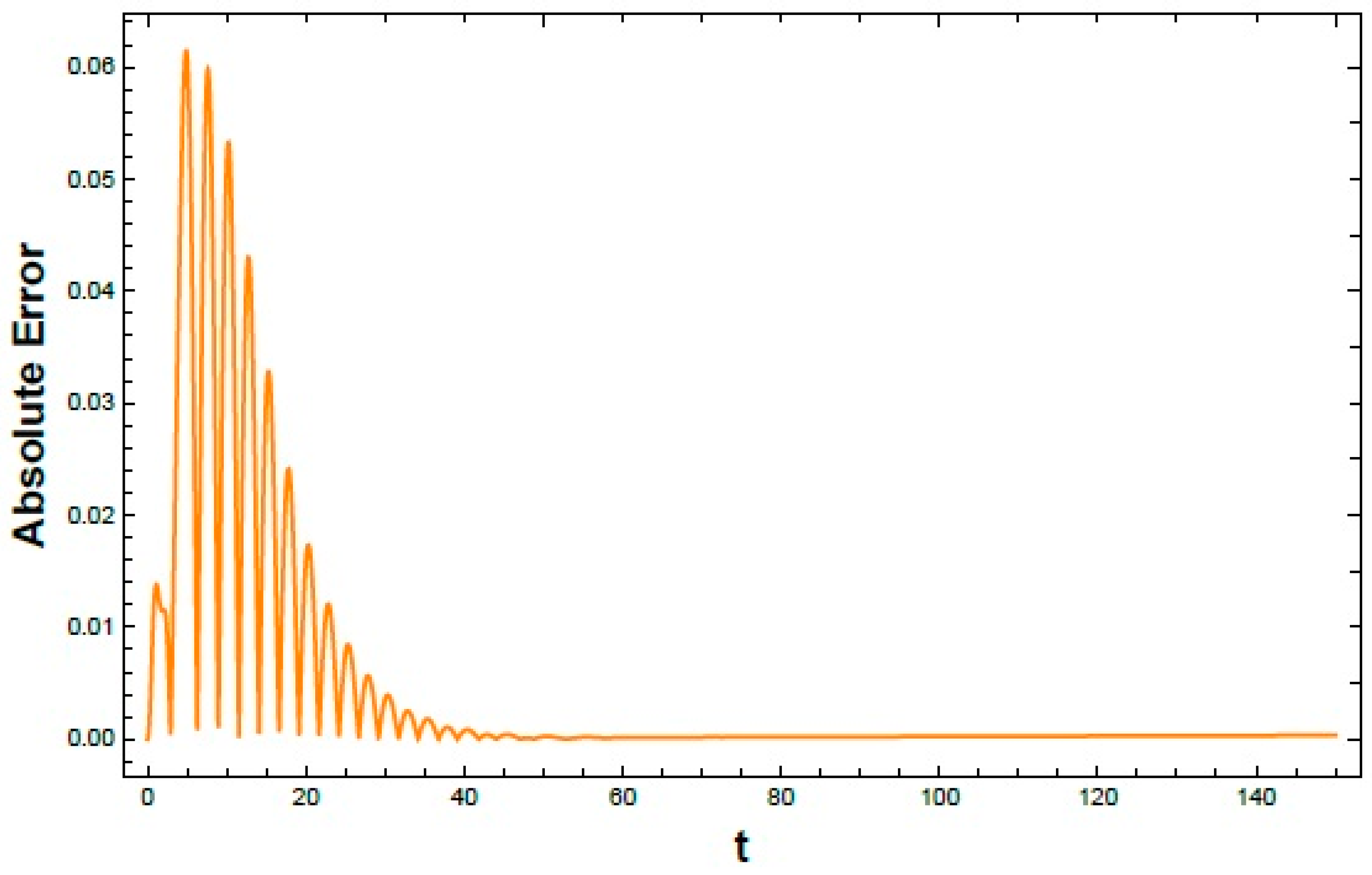
To quantify the discrepancy between the analytical and NSs, the Absolute error is shown in Figure 6. The error remains small over the entire simulation interval $t\in \left[0, 150\right]$, indicating overall agreement between both solutions. A slight increase appears in the initial transient stage due to nonlinear effects. As the system approaches a steady state, the error becomes nearly bounded within a narrow oscillatory range, with no sign of divergence. These results indicate consistent agreement between both methods within the weak-to-moderate nonlinear regime and support the applicability of the proposed NPA for subsequent analyses.

Figure 6. Shows the time evolution of the absolute errors between the NS and NPA solutions for NES.

4.3. Error Analysis and Numerical Accuracy Based on Tabulated Results

The error analysis presented in Table 3, Table 4 and Table 5 provides a quantitative assessment of the accuracy of the proposed NPA by comparison with the direct numerical solution under variations of three key system parameters: the primary oscillator amplitude, the primary damping coefficient, and the linear coupling stiffness. The results reveal a systematic dependence of the error measures on these parameter variations. Within the investigated parameter ranges, increasing the primary oscillator amplitude and the linear coupling stiffness is associated with gradual increases in the Maximum Absolute Error (Max Error), Root Mean Square Error (RMSE), and Mean Absolute Error (MAE). In contrast, increasing the primary damping coefficient leads to a consistent reduction in all three error measures. These results indicate that the approximation accuracy varies in a predictable manner with the selected system parameters while maintaining close agreement with the direct numerical solution over the investigated parameter ranges considered in this study.

Table 3. Variation of Error Metrics (Max Error, RMSE, and MAE) with diverse values of amplitude of primary oscillator over the interval $t\in \left[0, 150\right]$.

$\mathbf{A}$	Max Error	RMSE	MAE	${\mathbf{R}}^2$
0.2	0.00326703	0.00130437	0.00109629	0.996691
0.4	0.00591775	0.00167869	0.00134181	0.998625
0.6	0.0130701	0.00297629	0.00197082	0.998078
0.8	0.0258531	0.00560683	0.00307239	0.996167
1.0	0.0457429	0.00980243	0.00475998	0.992512

Table 4. Displays variation of Error Metrics (Max Error, RMSE, and MAE) with diverse values of primary damping over the interval $t\in \left[0, 150\right]$.

${\mathit{\xi }}_1$	Max Error	RMSE	MAE
0.2	0.0531337	0.0138895	0.00759096
0.4	0.0250432	0.00484627	0.00246435
0.6	0.0174752	0.00265422	0.00152764
0.8	0.0115501	0.00181311	0.00124174
1.0	0.00732367	0.00146068	0.00112776

Table 5. Shows variation of Error Metrics (Max Error, RMSE, and MAE) with diverse values of linear coupling stiffness over the interval $t\in \left[0, 150\right]$.

${\mathit{\alpha }}_2$	Max Error	RMSE	MAE
0.2	0.0305012	0.00541447	0.00421169
0.4	0.0438538	0.00599337	0.00430803
0.6	0.0641595	0.00705671	0.00450148
0.8	0.0811356	0.00797218	0.00467794
1.0	0.0946575	0.00873261	0.00481801

4.4. Error Contour Mapping

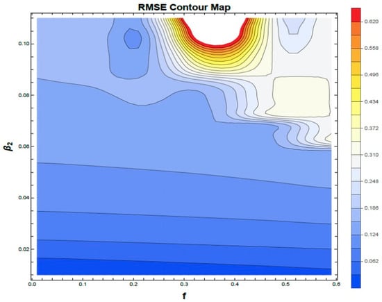
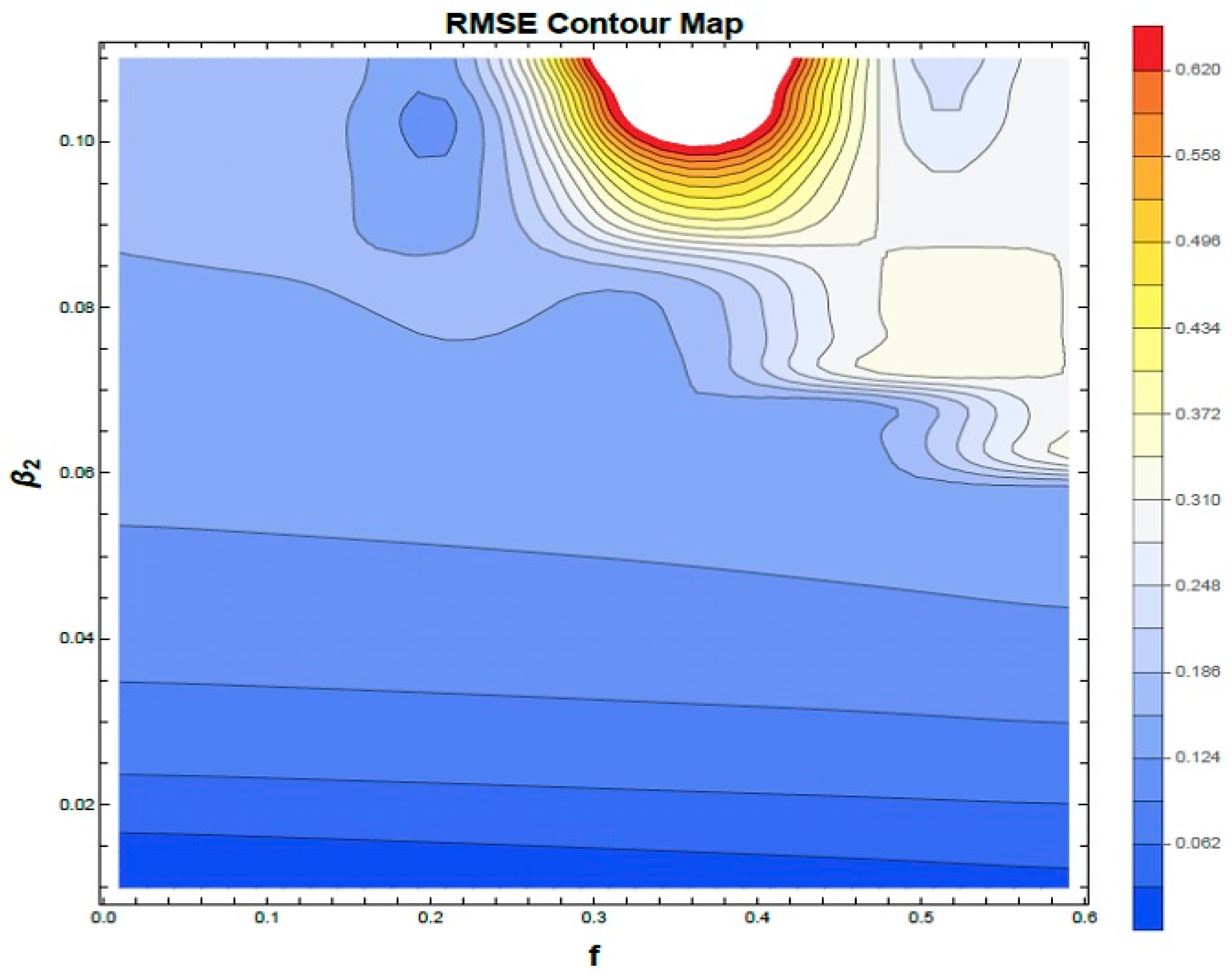
To assess the range of applicability of the proposed NPA, RMSE-based parameter-space analysis was performed by comparing the NPA predictions with direct numerical integration of the original nonlinear system. The investigation was carried out in the $\left(f,{\beta }_2\right)$ plane over the ranges $\left(f=0.01\to 0.60\right)$ and $\left({\beta }_2=0.01\to 0.12\right)$ while all remaining parameters were fixed at the baseline values adopted throughout the study. Figure 7 presents the RMSE contour map used to assess the validity range of the proposed NPA. The results indicate that the NPA maintains good agreement with the original nonlinear system over a wide region of the investigated parameter space. The approximation error increases gradually with higher forcing amplitude and nonlinear stiffness, reflecting the expected influence of nonlinear interactions. This behavior is consistent with the single-harmonic assumption adopted in the formulation, where higher-order harmonic effects are not explicitly represented.

Figure 7. Shows the RMSE contour map comparing the proposed NPA with the direct numerical solution over the $\left(f,{\beta }_2\right)$ parameter space. The fixed parameter values employed here are: $A=0.8, B=0.6, {\xi }_1=0.45,$ ${\xi }_2=0.05, \Omega =0.08,$ ${\beta }_1=0.2,$ and ${\alpha }_2=0.2$.

4.5. Comparison with Relevant Literature and Methodological Positioning

Gendelman and Bar [2] studied bifurcation phenomena in self-excited van der Pol oscillators coupled with a nonlinear energy sink, while the present work considers a harmonically forced primary oscillator coupled with a 2DOF-NES under external excitation. Starosvetsky and Gendelman [3,4,5] analyzed 1DOF-NES configurations, whereas the present study extends the system to a 2DOF attachment with additional coupling effects. Vakakis [6] introduced targeted energy transfer in linear primary systems, while the present formulation considers a nonlinear primary oscillator coupled with a 2DOF-NES under harmonic excitation. Taghipour and Dardel [7] applied the MCXA technique for steady-state analysis under moderate nonlinear assumptions. In contrast, the present work adopts a non-perturbative amplitude-dependent formulation that represents the nonlinear dynamics without harmonic truncation or small-parameter assumptions. This provides a unified analytical description of the system response and its stability behavior. Overall, the present formulation offers a consistent analytical framework for the coupled oscillator–NES system while preserving the full nonlinear structure of the governing equations.

5. Interpretation and Physical Significance

In this section, the stability characteristics are first identified from the total frequency–amplitude response and then verified using Floquet multipliers. Representative time-history responses, phase-plane trajectories, and polar representations are subsequently presented to illustrate the corresponding system dynamics.

5.1. Stability Analysis

To investigate the dynamics of the coupled 2DOF oscillator–NES, the influence of key physical parameters on stability is examined using the analytical conditions derived from the NPA (as shown in Equations (22) and (23)). Stability maps are constructed in the plane of total frequency versus initial amplitude using NSs in MS. The resulting plots distinguish stable (S) and unstable (U) regions corresponding to the derived transition curves, allowing visualization of the dependence of stability on system parameters. The dimensionless factors used in these simulations are: $\Omega =2.0, r=3.0$ ${\xi }_1=0.1,$ and ${\alpha }_2=2.0$.

5.1.1. Stability Analysis Under Constraint (22)

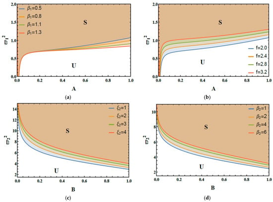
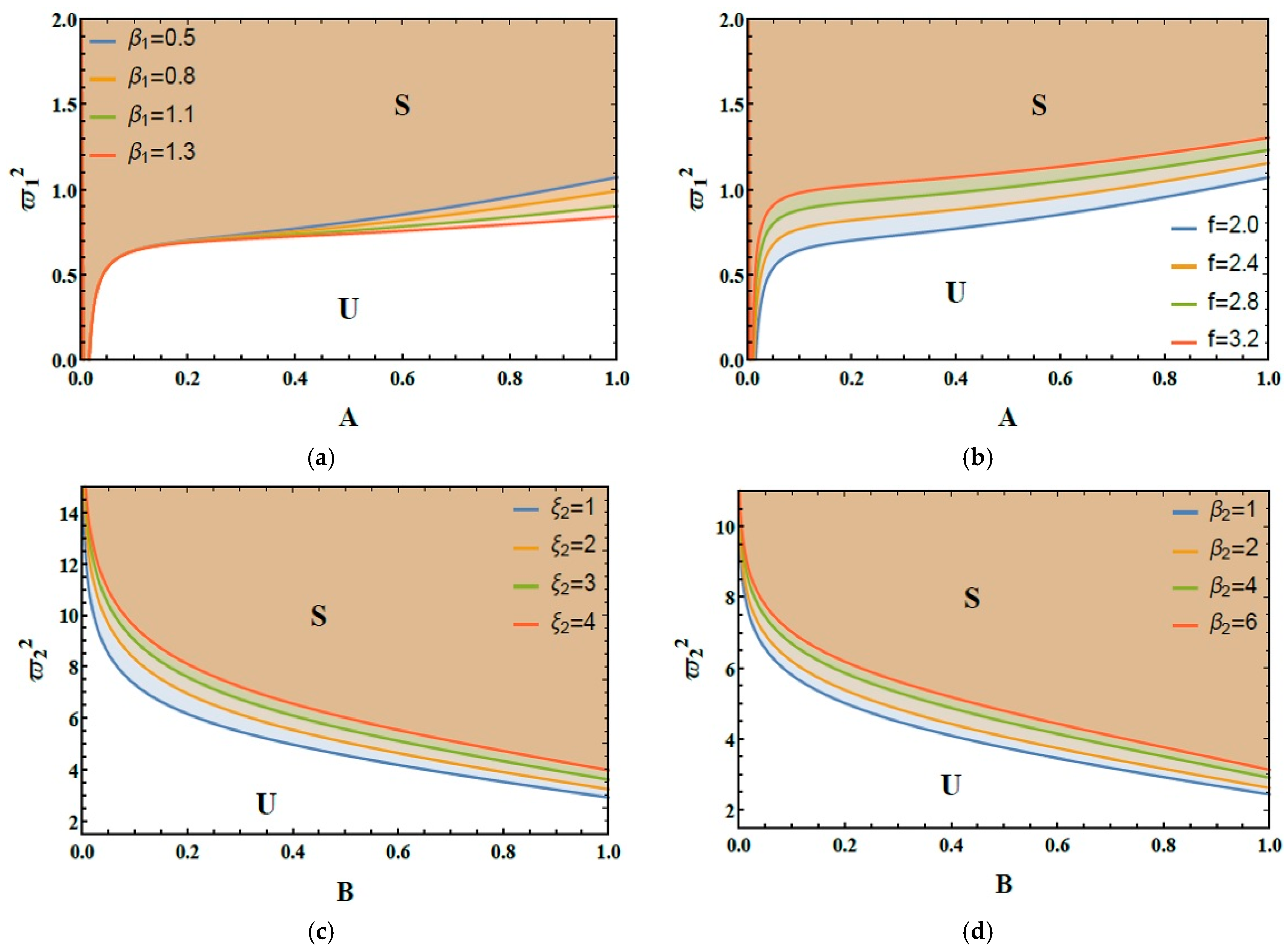
Figure 8a demonstrates the impact of the cubic nonlinearity factor ${\beta }_1$ on the system’s stability distribution. Increasing this parameter shifts the stability boundary toward higher initial amplitudes, indicating an enlarged bounded-response region under nonlinear stiffness. This reflects the influence of nonlinear restoring forces on the response amplitude and the resulting stability domain.

Figure 8. (a) Expounds the impact of ${\beta }_1$ on the stability zone. (b) Elucidates the role of $f$ on the stability picture. (c) Exposes the impact of ${\xi }_2$ on the stability schema. (d) Reflects the behavior of ${\beta }_2$ on the stability graph.

Figure 8b demonstrates the impact of the excitation force amplitude $f$ on stability distribution. As the excitation force amplitude $f$ escalates from 2.0 to 3.2, the stable region shrinks markedly, indicating a reduced range of ICs supporting bounded motion due to increased energy input into the primary oscillator.

5.1.2. Stability Analysis Under Constraint (23)

Figure 8c examines the role of the NES damping factor ${\xi }_2$ on the stability diagram. Escalating ${\xi }_2$ from 1.0 to 4.0 leads to a significant contraction of the stable zone, which can be attributed to reduced relative motion between the primary oscillator and the NES, thereby affecting the efficiency of nonlinear energy exchange.

Figure 8d demonstrates the performance of escalating the cubic coupling factor ${\beta }_2$ of the two oscillators on the stability profile. As ${\beta }_2$ escalates from 1.0 to 6.0, it modifies the stability boundaries and contributes to enlarging the region of the bounded response, reflecting nonlinear interaction between the subsystems.

The results presented in Figure 8a–d provide qualitative insights into the role of system parameters in shaping the stability characteristics of the coupled oscillator–NES system. It is observed that variations in damping, coupling stiffness, and excitation frequency significantly affect the distribution of stable and unstable regions through their impact on nonlinear energy exchange between the subsystems. These observations are intended to enhance the physical interpretation of the system dynamics rather than to establish explicit design or optimization guidelines. The present analysis is performed under nominal parameter conditions, while the effects of parameter uncertainties (such as manufacturing tolerances and environmental variations) are acknowledged but are beyond the scope of the present study and are left for future investigation.

5.1.3. Stability Evaluation via Floquet Theory

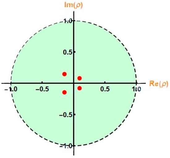
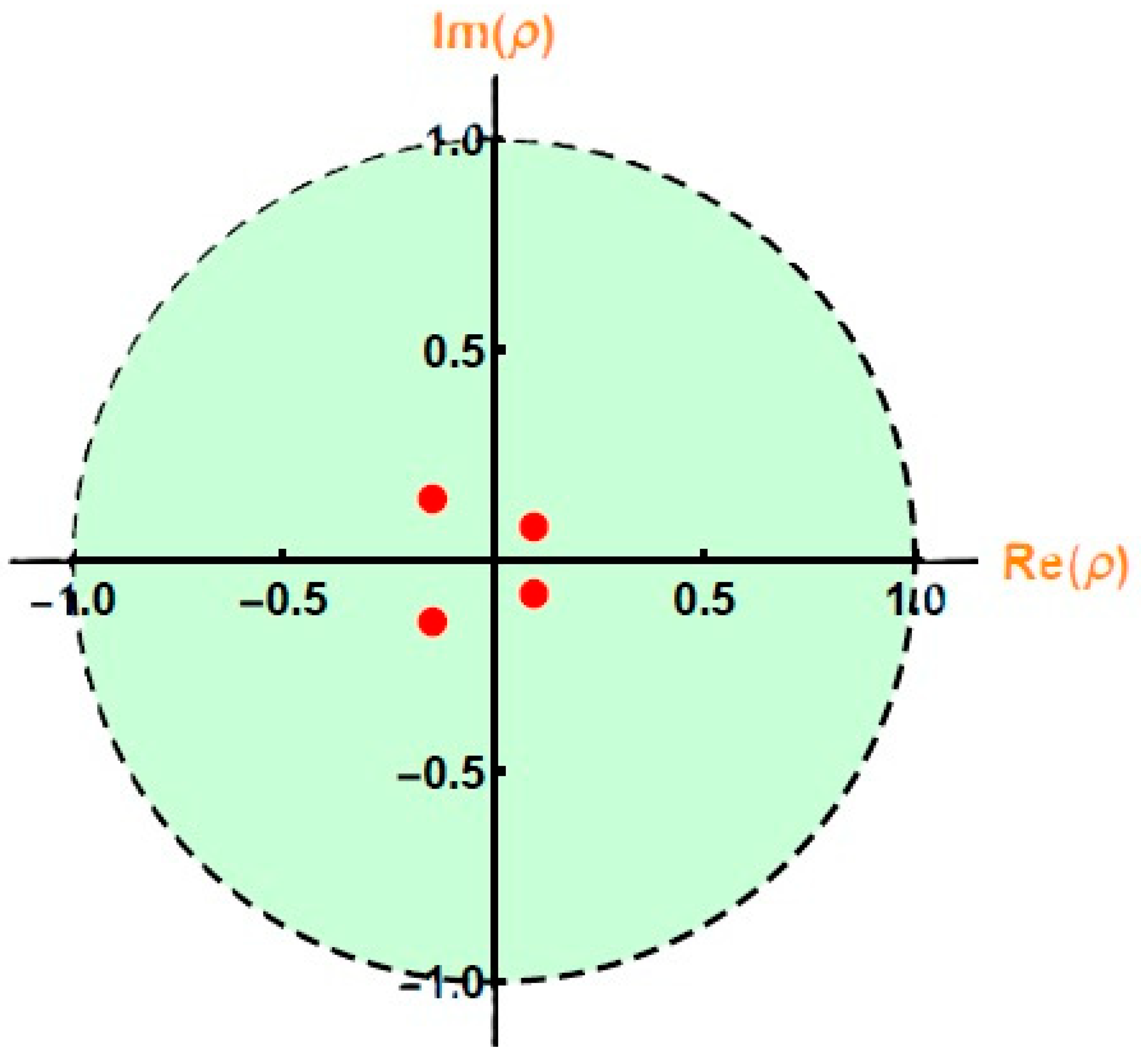
The Floquet multiplier analysis, shown in Figure 9, provides a quantitative verification of the periodic solution stability. The multipliers are plotted in the complex plane together with the unit circle, which serves as the stability boundary. It is observed that for stable regimes, all multipliers remain inside the unit circle, indicating asymptotic stability of the periodic orbit. In contrast, the crossing of multipliers outside the unit circle corresponds to loss of stability and the onset of bifurcation phenomena. This confirms the results obtained from BDs and LE analysis, and provides a rigorous validation of the stability transitions in the coupled nonlinear system. The fixed parameter values are: $A=0.25, B=0.30, {\xi }_1=2.5,$ ${\xi }_2=2.0, \Omega =0.6,$ ${\beta }_1=0.6, {\beta }_2=0.7$ and ${\alpha }_2=0.2$.

Figure 9. Displays Floquet multipliers (red dots) plotted on the complex plane. The dashed circle represents the unit circle.

5.1.4. Stability Tongues

In what follows, the stability tongues are analyzed for a system having the following particulars: $A=0.5, B=0.3, {\xi }_1=0.17$, ${\xi }_2=0.09$, ${\beta }_1=0.05, {\beta }_2=0.01$ and ${\alpha }_2=0.2$.

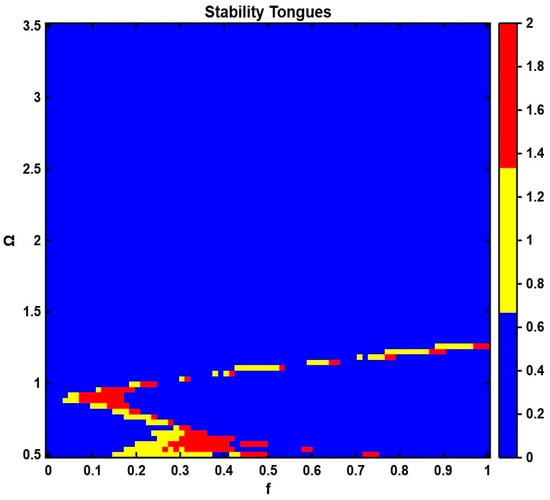
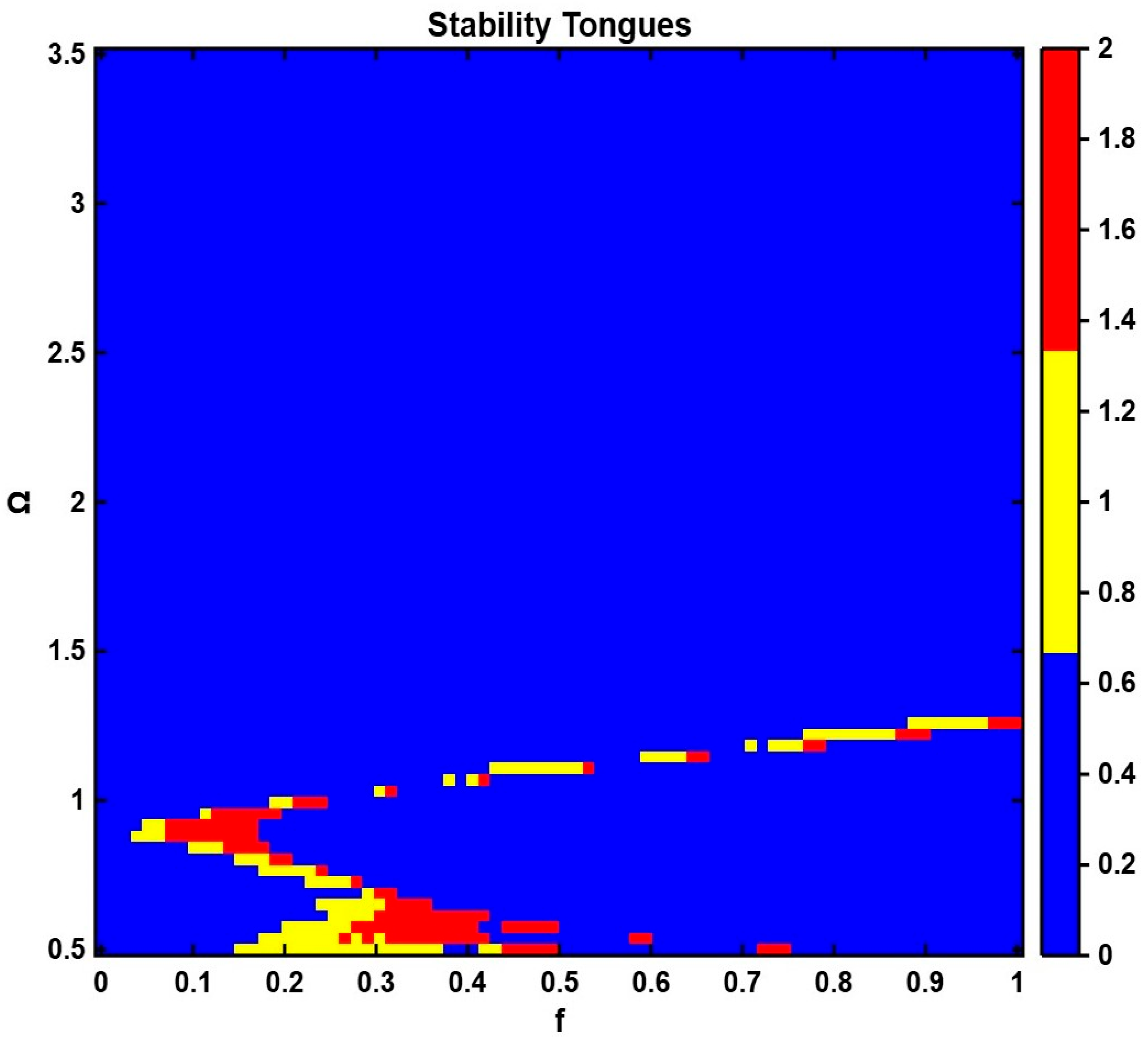
The stability characteristics of the coupled oscillator–NES are further illustrated using the stability tongues (Arnold tongues) diagram shown in Figure 10. The diagram presents the evolution of stable and unstable regions in the excitation amplitude–frequency parameter space. Stable periodic response regimes are observed in the blue regions, while red and yellow zones indicate the onset of instability and complex nonlinear dynamics. The results indicate that the stability boundaries are strongly dependent on both forcing amplitude and excitation frequency, highlighting the nonlinear interaction between the primary oscillator and the NES. The observed tongue-like structures are consistent with classical resonance phenomena in parametrically and harmonically excited nonlinear systems, reflecting multiple stability transitions as system parameters vary.

Figure 10. Demonstrates Stability tongues of the coupled oscillator–2DOF-NES system in the $\left(f,\Omega \right)$ plane, showing stable, transition (quasi-periodic), and unstable (chaotic) regions.

Overall, the obtained stability characteristics are not inferred solely from qualitative observations but are supported by transition-curve analysis, stability tongues, Floquet multiplier evaluation, BDs, and LE calculations.

5.2. Temporal Response Investigation

The time-domain responses are presented to illustrate the transient behavior of the coupled primary oscillator–2DOF-NES and to complement the stability results discussed in Section 5.1.

5.2.1. Response of the Primary Oscillator

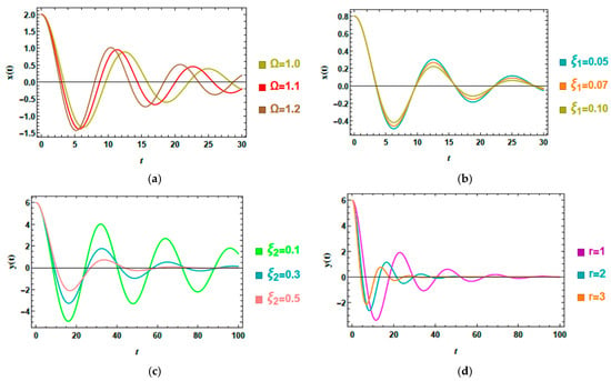
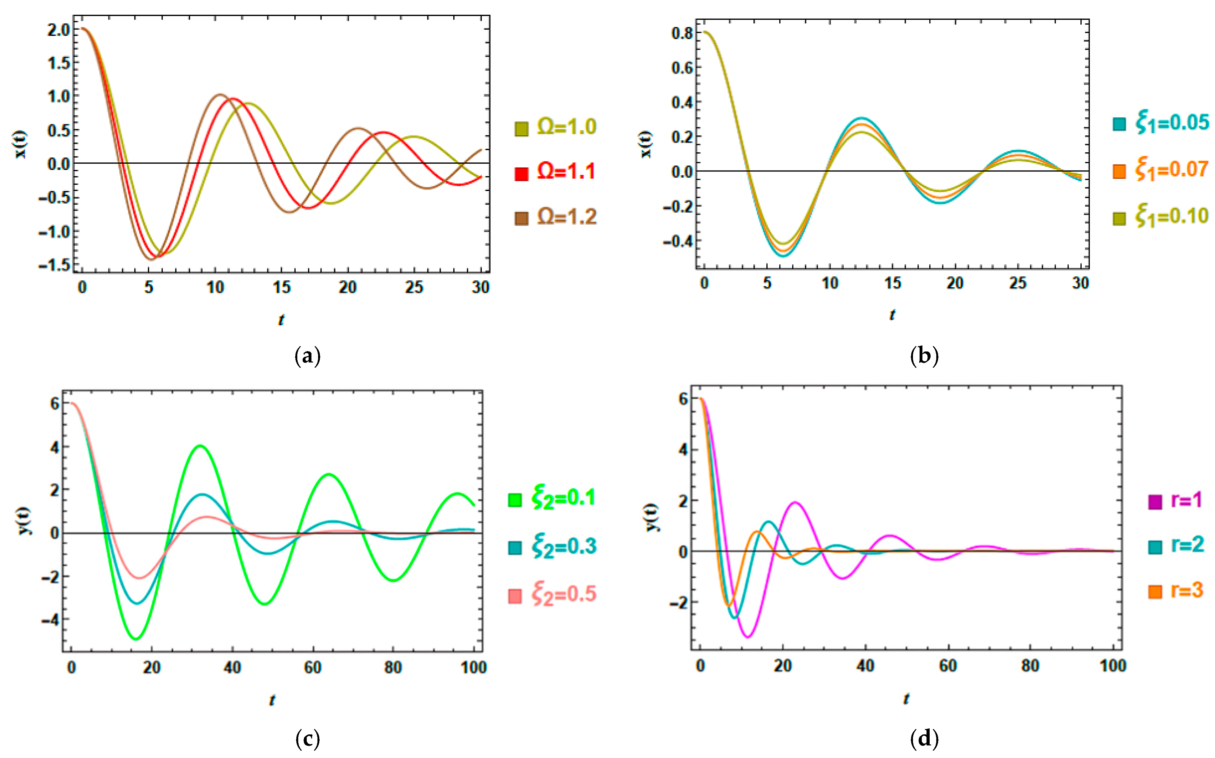
Figure 11a,b demonstrate the temporal response of the primary oscillator across various parameter modifications. The baseline dimensionless parameters are:

$$A=1.0, B=2.5, r=3, {\xi }_1=0.1, {\xi }_2=0.08, f=1.0,\Omega =2.0, {\beta }_1=0.01, {\beta }_2=0.01 \mathrm{and} {\alpha }_2=1.0.$$

Figure 11. (a) Shows the conduct of $\Omega$ on $x(t)$. (b) Elucidates the behavior of ${\xi }_1$ on $x(t)$. (c) Reflects the conduct of ${\xi }_2$ on $y(t)$. (d) Depicts the influence of $r$ on $y(t)$.

Figure 11a demonstrates the role of the excitation frequency $\Omega$ on the displacement response $x(t)$ of the primary oscillator. As the excitation frequency escalates, noticeable changes in the oscillation amplitude and decay characteristics are observed. This behavior is consistent with the stability trends discussed in Section 5.1, where variations in the excitation frequency modify the dynamic response characteristics of the coupled system. This behavior reflects the sensitivity of the coupled system to excitation frequency, which affects the dynamic interaction between the primary oscillator and the NES. The results indicate that frequency variations can significantly modify the transient response and attenuation characteristics of the coupled system.

Figure 11b depicts the influence of the intrinsic damping factor ${\xi }_1$ of the primary oscillator on the displacement response $x(t)$. As the damping coefficient increases, the oscillations decay more rapidly owing to enhanced dissipation. Conversely, lower damping values result in longer-lasting oscillations and slower attenuation. These observations indicate that the damping coefficient significantly influences the transient response characteristics of the coupled system. The obtained behavior is also consistent with the stability trends discussed in Section 5.1, where variations in damping modify the extent of the stable operating region.

5.2.2. Response of the NES

Figure 11c,d presents the time histories of the NES displacement, illustrating the dynamic response of the NES subsystem induced through its coupling with the primary oscillator. The fixed dimensionless parameters are: $A=3.0, B=6.0, 5, r=0.5,{\xi }_1=0.1,$ ${\xi }_2=0.2, f=1.0,\Omega =2.0$, ${\beta }_1=0.1, {\beta }_2=0.02$ and ${\alpha }_2=0.02$.

Figure 11c illustrates the effect of the NES damping coefficient $\left({\xi }_2=0.1, 0.3, 0.5\right)$ on the displacement response of the NES subsystem $y(t)$. As the damping coefficient increases, the oscillation amplitude decreases more rapidly, and the response reaches a bounded state within a shorter time interval. In contrast, lower damping values lead to more persistent oscillations and slower attenuation. These results indicate that the NES damping coefficient significantly influences the transient response characteristics of the coupled system and are consistent with the stability trends discussed in Section 5.1.

The influence of the mass ratio r on the displacement response of the NES subsystem $y(t)$ is clearly depicted in Figure 11d. Variations in the mass ratio produce noticeable changes in both the oscillation amplitude and attenuation characteristics. As the mass ratio increases, the response exhibits faster decay and reduced oscillation levels within the investigated parameter range. These results indicate that the mass ratio is an important parameter affecting the transient dynamics of the coupled system and are consistent with the stability characteristics discussed in Section 5.1.

5.3. Investigation of Phase Plane

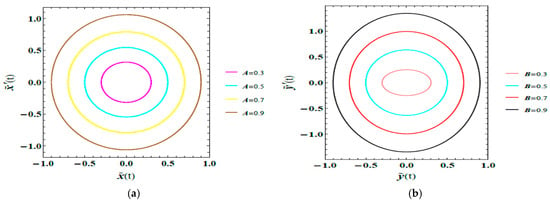
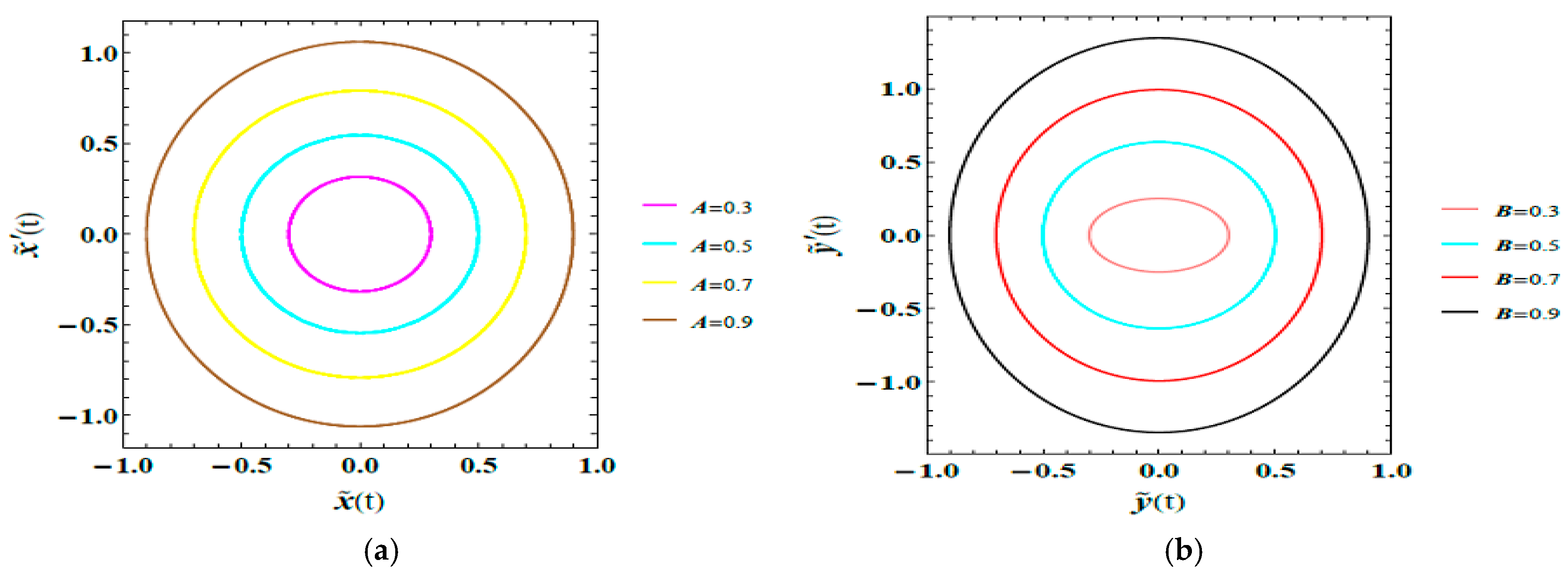
Phase-plane representations provide a qualitative description of the displacement–velocity response of the coupled primary oscillator–2DOF-NES. The geometry of the trajectories reflects the evolution of the system dynamics and facilitates visualization of bounded periodic motion, transient behavior, and the influence of parameter variations on the response characteristics. The phase portraits presented in Figure 12a,b are obtained using the dimensionless parameters, which are listed below:

$$f=1, \Omega =2.0, r=3.0,{\xi }_1=0.1, {\xi }_2=0.08, {\beta }_1=0.01, {\beta }_2=0.01 \mathrm{and} {\alpha }_2=1.$$

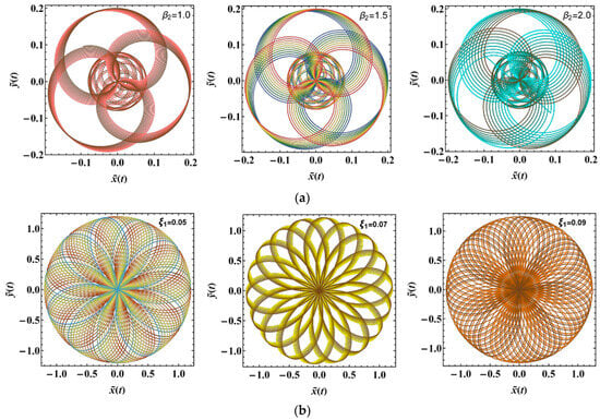
Figure 12. (a) Shows how $A$ affects the $\left(\tilde{u}, \dot{\tilde{u}}\right)$ plane. (b) Depicts the role of $B$ on the $\left(\tilde{v}, \dot{\tilde{v}}\right)$ plane.

Figure 12a depicts the phase portraits of the primary oscillator plane $\left(\tilde{u}, \dot{\tilde{u}}\right)$ for diverse values of $A$. As $A$ increases, the trajectories expand, indicating larger displacement and velocity levels. The progressive enlargement of the closed loops reflects the amplitude-dependent nonlinear response of the system arising from the cubic restoring terms. The observed changes in trajectory geometry demonstrate the increasing influence of nonlinear effects at higher oscillation levels while maintaining bounded periodic motion within the investigated parameter range.

Figure 12b displays the phase portraits of the NES plane $\left(\tilde{v}, \dot{\tilde{v}}\right)$ for different values of the amplitude $B$. As $B$ increases from 0.3 to 0.9, the trajectories become larger, reflecting higher displacement and velocity levels. The trajectories exhibit spiral-type behavior with progressively decreasing orbit size, indicating attenuation of the response within the considered parameter range. The observed evolution of the phase portraits demonstrates the influence of the nonlinear coupling on the NES dynamics and confirms that its response remains bounded throughout the investigated conditions.

5.4. Polar Response Analysis

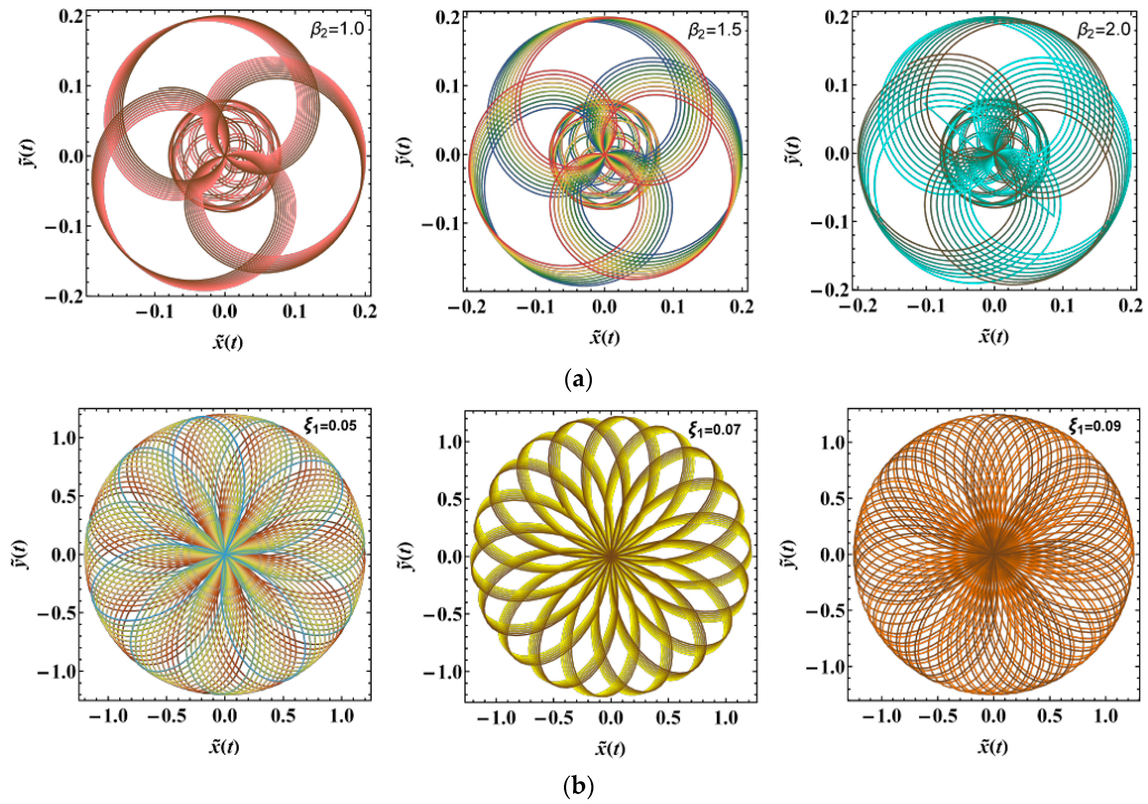
Figure 13a,b demonstrates the PolarPlots of the steady-state responses $\tilde{x}(t)$ vs. $\tilde{y}(t)$ under systematic variations of the governing factors ${\beta }_2$, and ${\xi }_1$. The responses are plotted after the decay of transient effects, so that the resulting trajectories represent the long-term dynamical behavior of the system. The polar representation provides an alternative visualization of the amplitude and phase evolution of the oscillatory response, offering additional qualitative insight into the nonlinear characteristics of the coupled primary oscillator–2DOF-NES. The dimensionless parameters used in these simulations are:

$$f=1, \Omega =0.5, r=0.5 {\xi }_1=2.0, {\xi }_2=0.2, {\beta }_1=0.1, {\beta }_2=1.5, A=0.08, B=0.2 \mathrm{and} {\alpha }_2=1.2.$$

Figure 13. (a) Expounds the PolarPlot schematic of $\tilde{x}(t)$ vs. $\tilde{y}(t)$ influenced by ${\beta }_2$. (b) Outlines the PolarPlot schematic of $\tilde{x}(t)$ vs. $\tilde{y}(t)$ influenced by ${\xi }_1$.

Figure 13a illustrates the effect of the cubic coupling parameter ${\beta }_2$ on the steady-state polar trajectories. As ${\beta }_2$ increases, the trajectories become more regular and exhibit a smoother, near-circular geometry. This change in the shape of the polar response reflects a more coherent periodic motion and highlights the influence of nonlinear coupling on the qualitative structure of the steady-state oscillations.

Figure 13b presents the performance of the primary damping factor ${\xi }_1$ on the steady-state polar trajectories. As ${\xi }_1$ increases, the radial extent of the trajectories changes, leading to variations in the overall size and shape of the polar orbits. This reflects the role of damping in modifying the amplitude characteristics of the steady-state response of the coupled system.

6. Basin of Attraction

Although damping generally promotes asymptotic stability, the presence of nonlinear coupling and internal energy transfer between the primary oscillator and the NES can lead to complex transient and long-term dynamics, including periodic windows, quasi-periodic responses, and chaotic motions. These performances are evaluated using direct numerical integration of the original nonlinear system and characterized through LE analysis. Motivated by this, a basin of attraction analysis is carried out to examine the sensitivity of the system to ICs and to identify regions of coexisting attractors.

In nonlinear dynamical systems, the long-term behavior of trajectories is dependent on their ICs. To investigate this sensitivity, basin of attraction analysis is employed as an effective tool for revealing multi-stability and the coexistence of different attractors. Conventionally, basins are constructed by identifying the asymptotic state reached from each initial condition, such as fixed points or periodic orbits [36,37].

In this analysis, the system dynamics are obtained through direct numerical integration of the full nonlinear governing equations over a grid of initial conditions. For each trajectory, the LLE is then computed to classify the resulting behavior. Positive LLE values indicate chaotic motion; zero values correspond to quasi-periodic responses, while negative values are associated with periodic or asymptotically stable solutions.

This approach provides a consistent and systematic way to distinguish between different types of dynamical behavior. By evaluating the LLE over a range of ICs, the transition from regular (periodic or quasi-periodic) motion to chaotic dynamics can be clearly identified. The resulting Lyapunov-based basin maps not only separate chaotic and non-chaotic regions but also provide useful insight into multi-stability and the sensitivity of the system to initial conditions in nonlinear dynamical regimes.

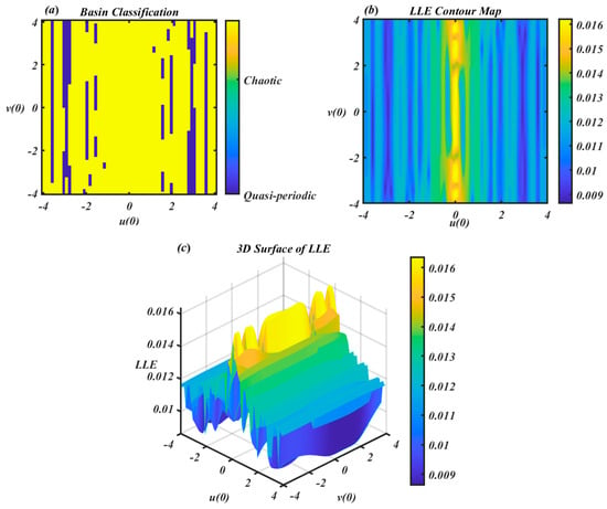
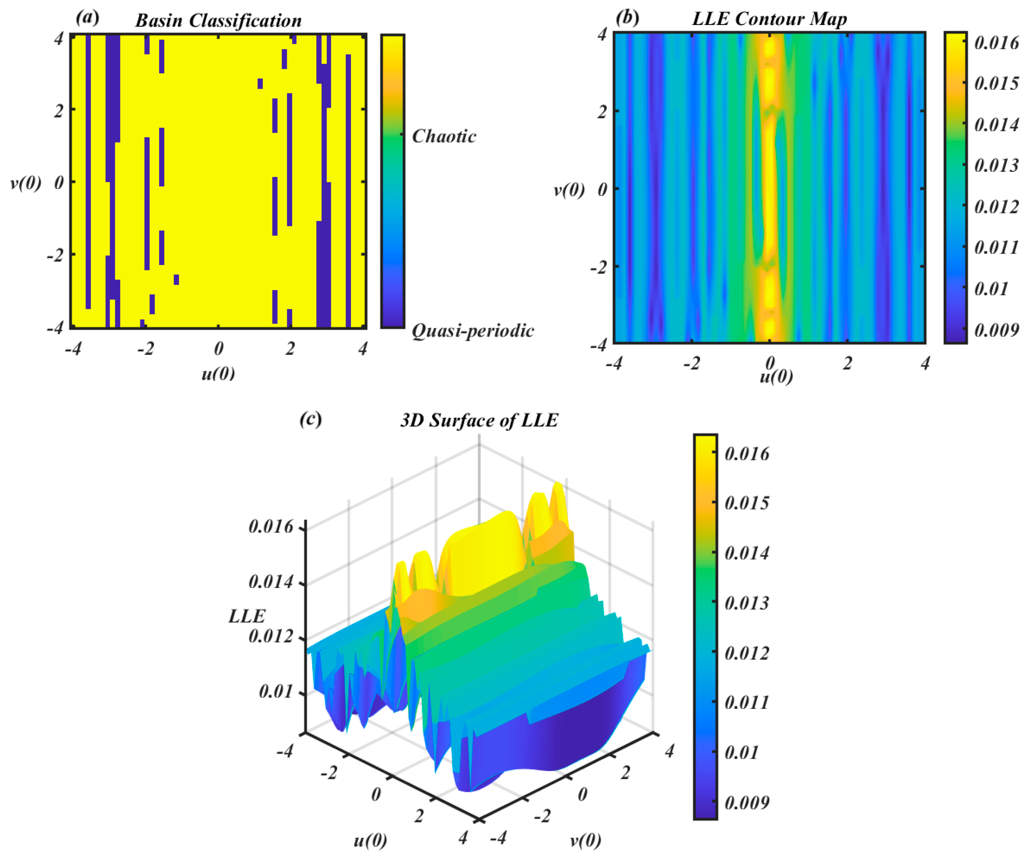
The basin of attraction analysis shown in Figure 14 provides a comprehensive understanding of the system’s sensitivity to ICs under the specified parameter set: ${\beta }_1=0.1,{\beta }_2=0.049, {\alpha }_2=5, {\xi }_1=5, {\xi }_2=3$, and $r=1$.

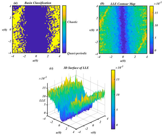
Figure 14. Shows Lyapunov based basin classification and LLE maps in $u(0)$, and the v(0) plane.

The dynamics are governed by the same nonlinear coupled system of ODEs with cubic, quadratic, and nonlinear coupling terms. The analysis explores the effect of varying the ICs as $u(0)$, and $v(0)$ over the range $[-4,4]$, while keeping the other initial conditions fixed.

In Figure 14a displays the basin classification map, where each pixel corresponds to a pair of ICs as $u(0)$, and $v(0)$ is color-coded based on the dynamic behavior determined via the LLE: yellow for chaotic motion and dark blue for quasi-periodic motion. The distribution reveals that $30.7\%$ of the ICs lead to chaotic behavior, while $69.3\%$ result in quasi-periodic responses. This indicates that the system is predominantly stable but exhibits significant chaotic regions, particularly near the periphery of the phase space. The presence of fine-grained interwoven structures between chaotic and quasi-periodic zones reflects the fractal boundary typical of multi-stable nonlinear systems, highlighting their sensitivity to ICs.

Figure 14b, the LLE contour map, provides a continuous representation of the LLE values across the same IC space. Higher LLE values (yellow) represent chaotic regions, while lower values (blue) indicate regular or quasi-periodic behavior. This smooth gradient visually captures the transition between order and chaos, with the central region remaining dominantly stable and the outer regions growing increasingly unstable. Figure 14c enhances this interpretation with a 3D surface plot of the LLE, where peaks in the landscape correspond to zones of high instability (chaotic behavior), and troughs indicate low LLE values associated with regular dynamics. This spatial profile further confirms that the basin structure is not uniform; instead, it features local instabilities embedded within broader stable zones.

In conclusion, the basin of attraction reveals the coexistence of quasi-periodic and chaotic attractors, with chaotic behavior occupying approximately 30.7% of the considered initial condition space based on the LLE-based classification. The resulting basin structure exhibits irregular boundaries and a non-uniform distribution of the LE, indicating the presence of multi-stability and sensitivity to ICs. These features are of particular importance in the design and control of nonlinear engineering systems, especially in applications such as MEMS and energy harvesting, where robustness and predictability are critical.

The three panels in Figure 15 provide a comprehensive depiction of the basin of attraction and underlying dynamical behavior of a four-dimensional nonlinear system, governed by the following parameter values:

$${\beta }_1=5\times {10}^{-5},{\beta }_2=5\times {10}^{-5}, {\alpha }_2=2\times {10}^{-4}, {\xi }_1=2\times {10}^{-4}, {\xi }_2=0.015, \mathrm{and} r=5.5.$$

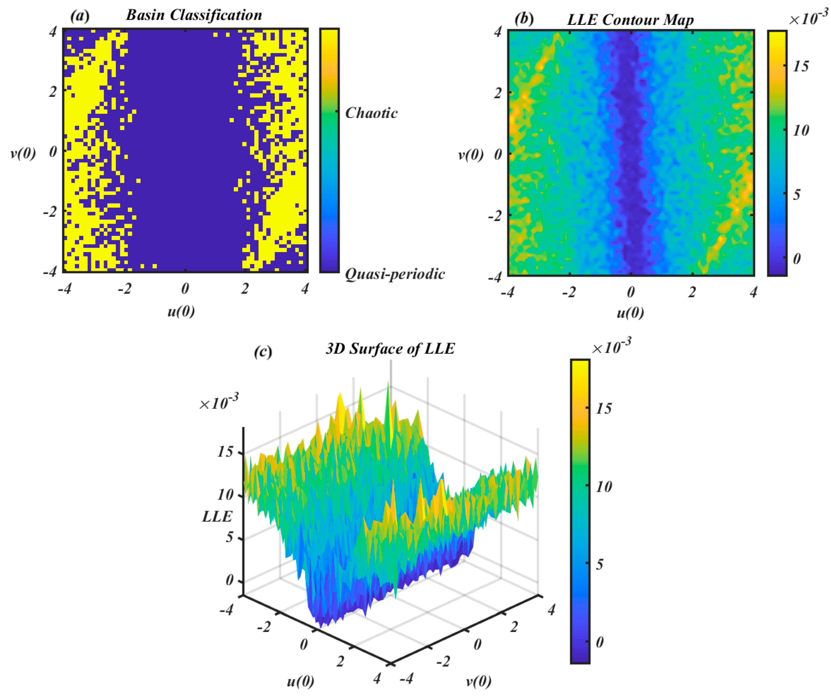
Figure 15. Shows Lyapunov based basin classification and LLE maps in $u(0)$, and v(0).

These parameters define a system capable of generating both chaotic and quasi-periodic trajectories depending on the ICs. Figure 15a shows the basin classification map, where each point in the $u(0)$, and $v(0)$ plane is color-coded according to the long-term behavior of the corresponding trajectory. Yellow regions correspond to chaotic responses, while dark blue regions indicate quasi-periodic motion. The map reveals that chaotic dynamics dominate the IC space, occupying approximately $86\%$ of it, with quasi-periodic trajectories occurring only in narrow, isolated regions comprising about $14\%$ of the basin. Moreover, the panel in Figure 15b presents the contour map of the LLE computed for each IC. Higher LLE values (yellow and orange hues) confirm the presence of chaotic dynamics, whereas lower LLE values (blue and green shades) identify regions of quasi-periodic behavior. This panel not only supports the classification shown in Figure 15a, but also captures the gradient transitions between dynamical regimes, indicating sensitivity near the boundaries. Figure 15c provides a 3D surface plot of the LLE over the same IC space, offering a topographic perspective of the system’s dynamical response. Peaks in the surface correspond to ICs with high LLEs (chaotic), while troughs represent zones of low LLEs (quasi-periodic). The combined results across all three panels demonstrate a multi-stable nature and pronounced sensitivity to initial conditions.

7. Chaotic and Bifurcation Analysis

Chaotic and bifurcation analyses provide complementary tools for characterizing the qualitative changes in the system dynamics under parameter variations. Bifurcation diagrams illustrate the evolution of asymptotic system responses with respect to the control parameter, while the LLE is used as a quantitative measure to distinguish between regular and chaotic behavior. Together, these tools provide a consistent framework for identifying transitions between different dynamical regimes [38]. The LLE was computed using this equation and the standard method of Benettin et al. [39]. The associated variational equations were integrated simultaneously with the main equations using a 4th-order Runge–Kutta method with a fixed time step of $\Delta t=X$. A Gram-Schmidt re-normalization procedure was applied for each $\tau =Y$ time unit. The exponents were averaged across $N=Z$ time units after eliminating an initial transient of $T_{\mathrm{trans}}$ to ensure convergence to the attractor. Custom MATLAB scripts were used for all numerical simulations, bifurcation studies, and LE computations. In nonlinear dynamical systems, a periodic window within a chaotic domain often occurs when:

• A stable and an unstable periodic orbit collide and annihilate during the saddle-node bifurcation of limit cycles, briefly allowing a periodic solution to prevail until chaos reemerges.
• Before the window, the system moves in a nearly periodic fashion interspersed with chaotic bursts; inside the window, it becomes completely periodic. It is defined by the sporadic path to anarchy. In parameter space, a phenomenon is called a “window.”
• When the external stimulation frequency locks onto a super harmonic or sub harmonic of the system’s inherent frequency, the system may briefly settle into periodic motion.

The nonlinear dynamical system considered in this study demonstrates rich and complex behavior as the control parameter $r$ varies over the interval $[0.042,0.215]$. Governed by coupled nonlinear differential equations incorporating cubic and quadratic nonlinearities, the system includes parameters

$${\beta }_1=5\times {10}^{-5},{\beta }_2=5\times {10}^{-5}, {\alpha }_2=2\times {10}^{-4}, {\xi }_1=2\times {10}^{-4}, {\xi }_2=0.015, \mathrm{and} r=5.6.$$

Figure 16 appears to illustrate a transient response. In contrast, Figure 16a,b are bifurcation diagrams, which represent the asymptotic, long-term behavior of the system as the parameter $r$ varies; after all initial transients have dissipated. Visually, subfigure (Figure 16a) shows distinct stable states for lower values of $r$; represented by a single line corresponding to a fixed point or periodic orbit, which then expands into a chaotic region at higher $r$ values, where the points become densely scattered. This characteristic structure indicates an asymptotic bifurcation diagram. If the figure primarily captured transient behavior, one would expect less organization, more irregular fluctuations, or difficulty in identifying consistent patterns. Instead, the chaotic region is well-defined and thoroughly populated, suggesting that transients have settled and the system’s long-term dynamics are displayed.

Figure 16. (a) the bifurcation diagram for the solution $u$ versus $r$, (b) the bifurcation diagram for the solution $v$ against $r$, (c) the related Lyapunov spectrums.

Visually, Figure 16a shows well-defined stable states at lower values of $r$, represented by a single line corresponding to either a fixed point or a periodic orbit. As $r$ increases, this single branch expands into a chaotic regime, where the points become densely scattered. Such a structure is typical of an asymptotic bifurcation diagram. If the figure were dominated by transient behavior, the plot would appear less organized, with irregular fluctuations and no consistent patterns. However, the chaotic region here is well-developed and thoroughly populated, indicating that transient effects have largely decayed and the system’s long-term dynamics are being captured.

Regarding figure (Figure 16c): For values of $r$ below approximately 0.18, the leading LE ${\lambda }_1$ (red curve) is slightly negative, indicating stable dynamics consistent with the single-line attractors observed in Figure 16a,b. As $r$ increases into the range of about 0.18 to 0.2, ${\lambda }_1$ approaches and briefly touches zero, marking the onset of bifurcations such as period-doubling transitions toward chaos. When $r$ exceeds roughly 0.2, ${\lambda }_1$ becomes clearly positive, reaching values up to about 0.25, confirming the emergence of chaotic behavior. This aligns well with the scattered regions seen in the corresponding bifurcation diagrams for the same range of $r$. The vertical scale of figure (Figure 16c), extending from −3 to 0.5, provides sufficient resolution to distinguish negative from positive values, and the red curve can be seen rising above zero in the chaotic regime.

Therefore, the leading Lyapunov exponent can be readily interpreted from the given scale, making it easy to distinguish between its positive and negative values. It displays a clear transition from negative (indicating stable behavior) to positive (indicating chaotic performance) as $r$ escalates, which is essential for understanding the system’s dynamical evolution.

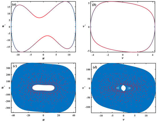
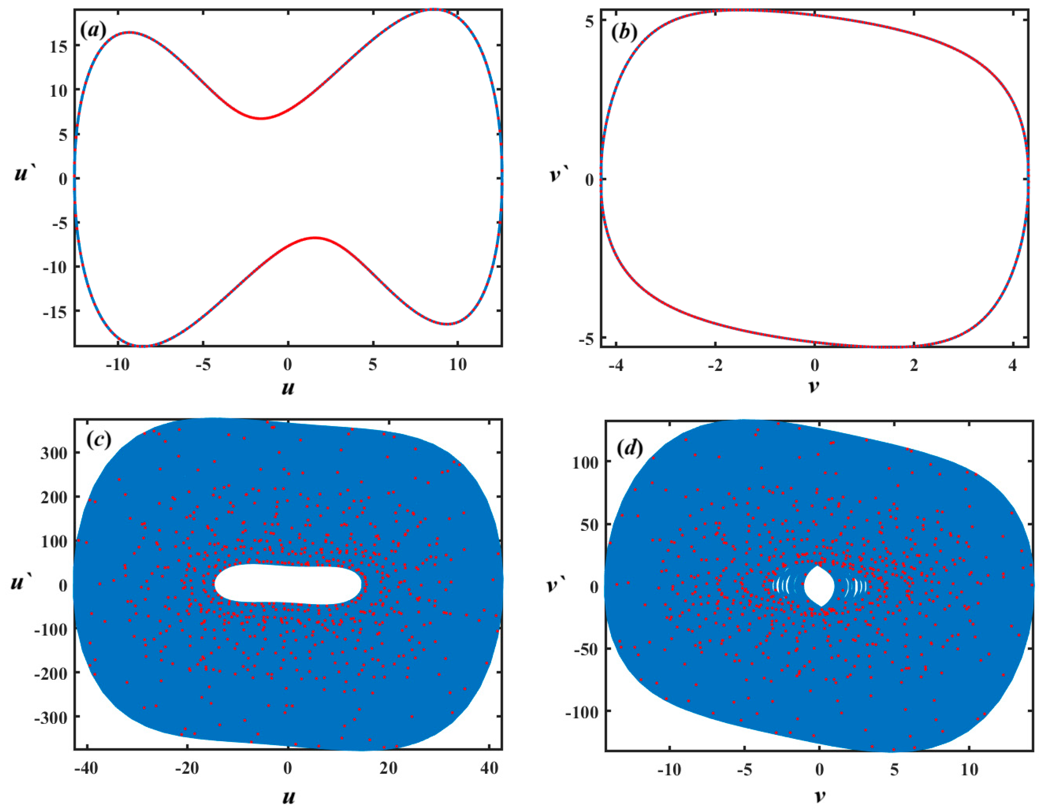
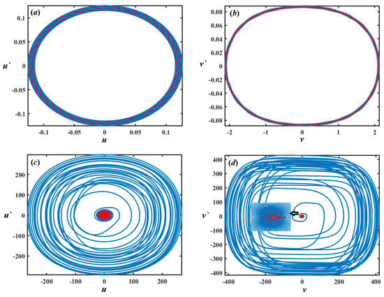
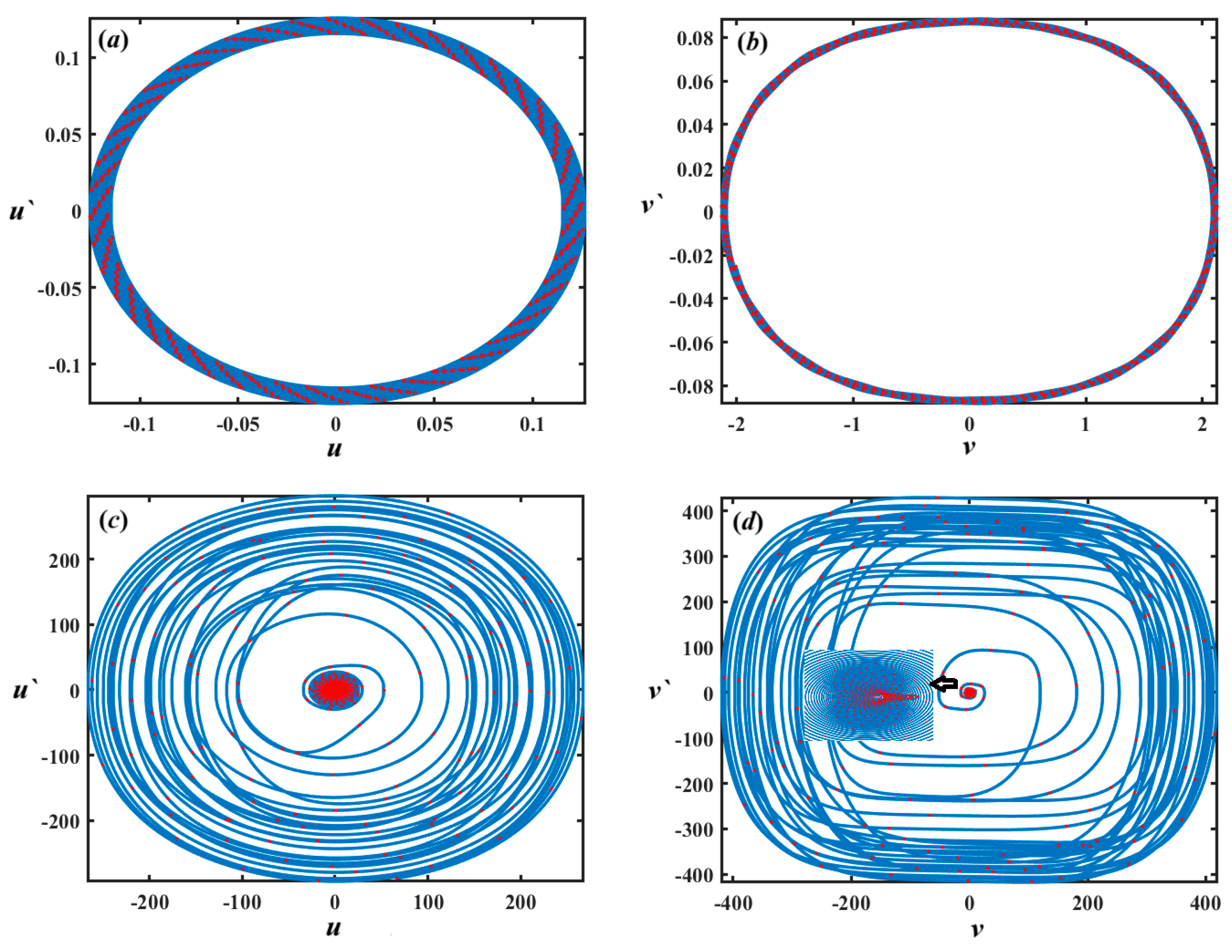
Analysis of Figure 17 can be demonstrated as follows: It is evident that the system’s response is notably influenced by the variation of the parameter $r$. When $r=0.042$, the system displays quasi-periodic motion, characterized by smooth, non-repeating oscillations that remain confined within a well-defined region of the phase space, as in the Figure 17a,b. This type of behavior suggests the coexistence of multiple incommensurate frequencies, leading to a structured yet non-periodic response. The trajectories in this case typically form closed loops or toroidal shapes in the phase space, indicating a stable and predictable dynamic pattern over time. In contrast, when the parameter escalates to $r=0.215$, the system enters a chaotic regime, as indicated in Figure 17c,d. This transition is marked by the breakdown of the quasi-periodic structure and the emergence of irregular, aperiodic oscillations. The motion becomes highly sensitive to ICs, and the phase space reveals a dense and erratic trajectory distribution, which is indicative of deterministic chaos. This shift from quasi-periodicity to chaos as $r$ elevates underscores the nonlinear nature of the system and highlights the critical role of parameter tuning in influencing its long-term behavior.

Figure 17. Diagrams of Poincaré maps and phase portraits for the solutions $u$, and $v$: (a,b) at $r=0.042$, (c,d) at $r=0.215$.

The nonlinear system, defined by a set of coupled ODEs with cubic and quadratic nonlinearities, is analyzed here by varying the parameter ${\xi }_2$ in the range $[0,0.0161]$ while keeping other parameters fixed:

$${\beta }_1=5\times {10}^{-5},{\beta }_2=5\times {10}^{-5}, {\alpha }_2=2\times {10}^{-4}, {\xi }_1=2\times {10}^{-4}, {\xi }_2=0.015, \mathrm{and} r=5.6.$$

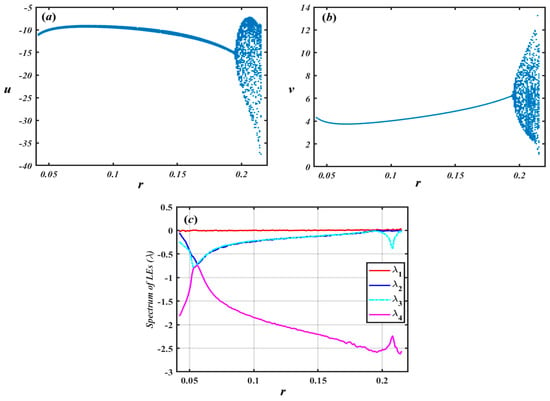
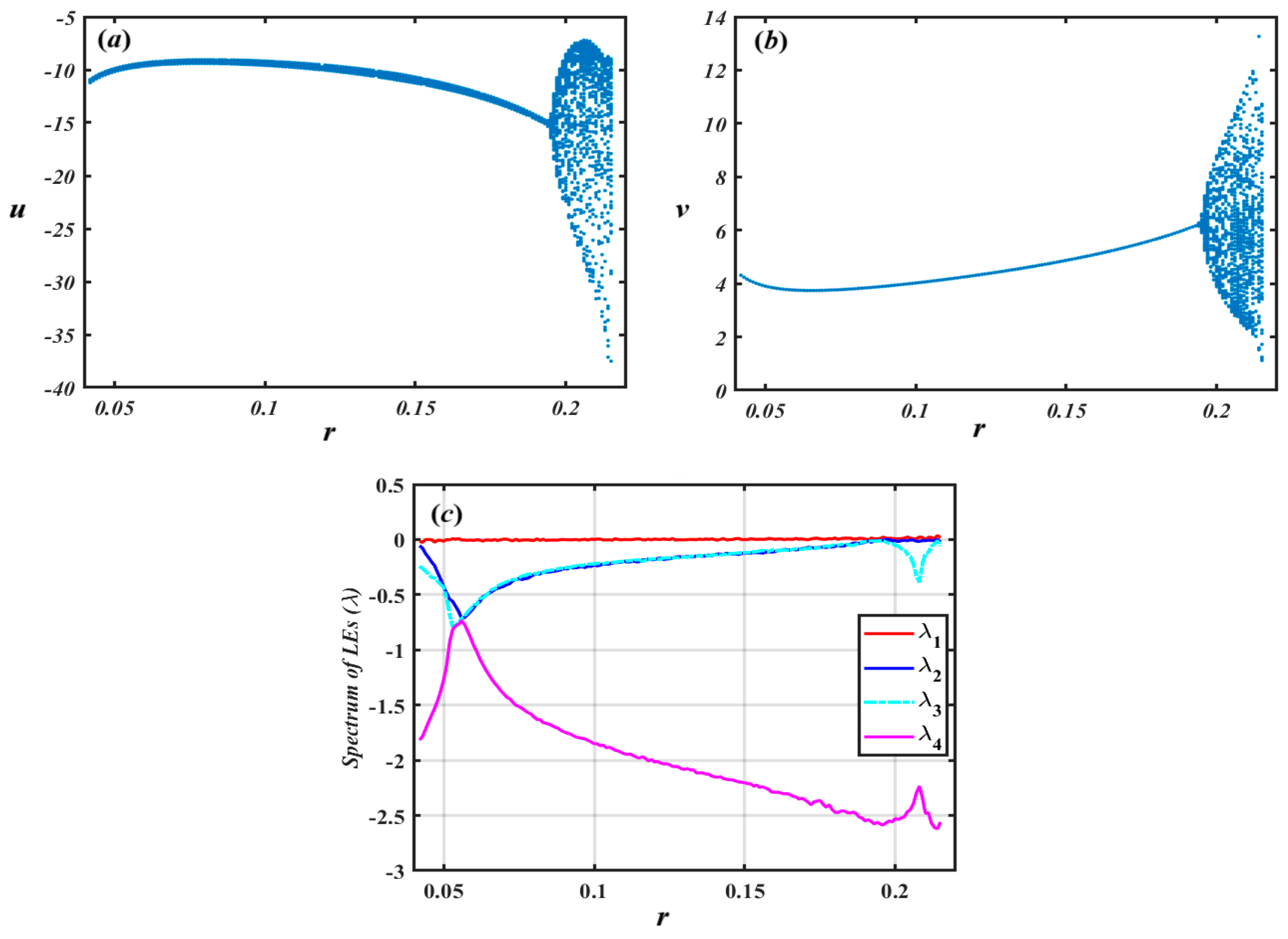
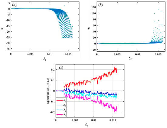
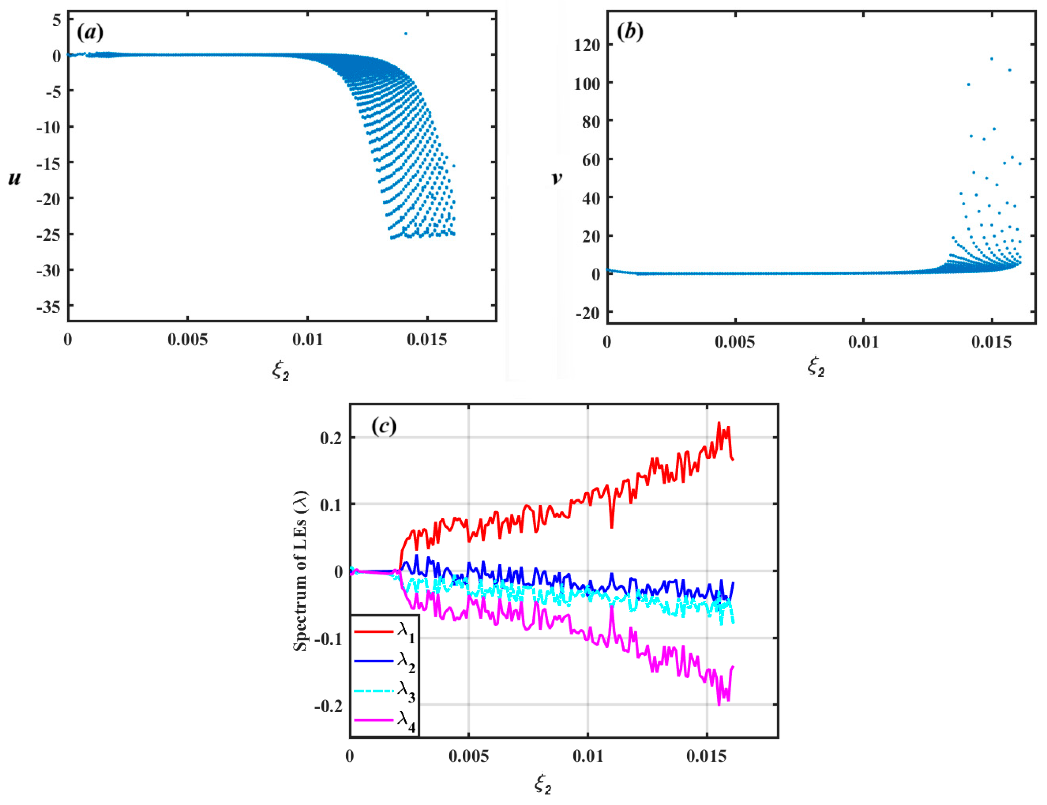
A closer inspection of Figure 18 shows that the bifurcation diagrams of the variables $u$ and $v$ show clear signs of period-doubling bifurcations as ${\xi }_2$ increases, as seen in Figure 18a,b. Initially, the system exhibits a stable periodic response for small values of ${\xi }_2$, but as ${\xi }_2$ exceeds approximately $0.005$, the solution branches begin to split repeatedly, leading to the emergence of complex periodic and chaotic patterns. This indicates a classical route to chaos via successive period doublings. The LEs spectrum further confirms the onset of chaos, as demonstrated in Figure 18c. For low values of ${\xi }_2$, all exponents are negative or zero, indicating stability or quasi-periodicity. However, as ${\xi }_2$ enlarges, the largest exponent ${\lambda }_1$ gradually rises and becomes positive, which is a definitive indicator of chaotic dynamics due to the exponential divergence of nearby trajectories in phase space. At the same time, the remaining exponents ${\lambda }_2, {\lambda }_3,$ and ${\lambda }_4$ remain negative, implying that the system possesses a single expanding direction and multiple contracting directions, a typical signature of a strange attractor in low-dimensional chaotic systems. The interplay between the bifurcation structure and the LE spectrum provides evidence of the system’s transition from order to chaos, highlighting the sensitivity of the system’s dynamics to the control parameter ${\xi }_2$. This analysis is crucial in the context of nonlinear control, energy harvesting, and MEMS/NEMS applications, where such dynamic transitions can significantly affect system performance and must be carefully managed or exploited.

Figure 18. (a) the bifurcation diagram for the solutions $u$ via ${\xi }_2$, (b) the bifurcation diagram for the solutions $v$ against ${\xi }_2$, (c) the related Lyapunov spectrums.

As evident from Figure 19, the dynamic behavior of the system significantly changes with variations in the parameter ${\xi }_2$. When ${\xi }_2=0.00016$, the system exhibits quasi-periodic behavior, as indicated in Figure 19a,b. This is characterized by oscillations that do not repeat exactly but maintain a structured and bounded trajectory in phase space, typically forming closed invariant curves or tori. Such behavior indicates the presence of multiple incommensurate frequencies governing the motion, which prevents the system from settling into a simple periodic orbit. However, as the value of ${\xi }_2$ increases to ${\xi }_2=0.016$, the system transitions to chaotic behavior, as noted in Figure 19c,d. In this regime, the trajectories become highly sensitive to initial conditions, leading to irregular and unpredictable motion over time. The corresponding phase portraits become more complex, often filling regions of phase space in an apparently random manner, which is a hallmark of chaos. This transition from quasi-periodicity to chaos highlights the critical role of the parameter ${\xi }_2$ in shaping the nonlinear dynamics of the system.

Figure 19. Diagrams of Poincaré maps and phase portraits for the solutions $u$, and $v$: (a,b) at ${\xi }_2=0.00016$, (c,d) at ${\xi }_2=0.016$.

Now, let us consider the action of the excitation force that acted on the examined model (Figure 1).

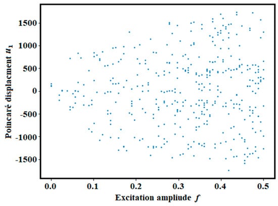
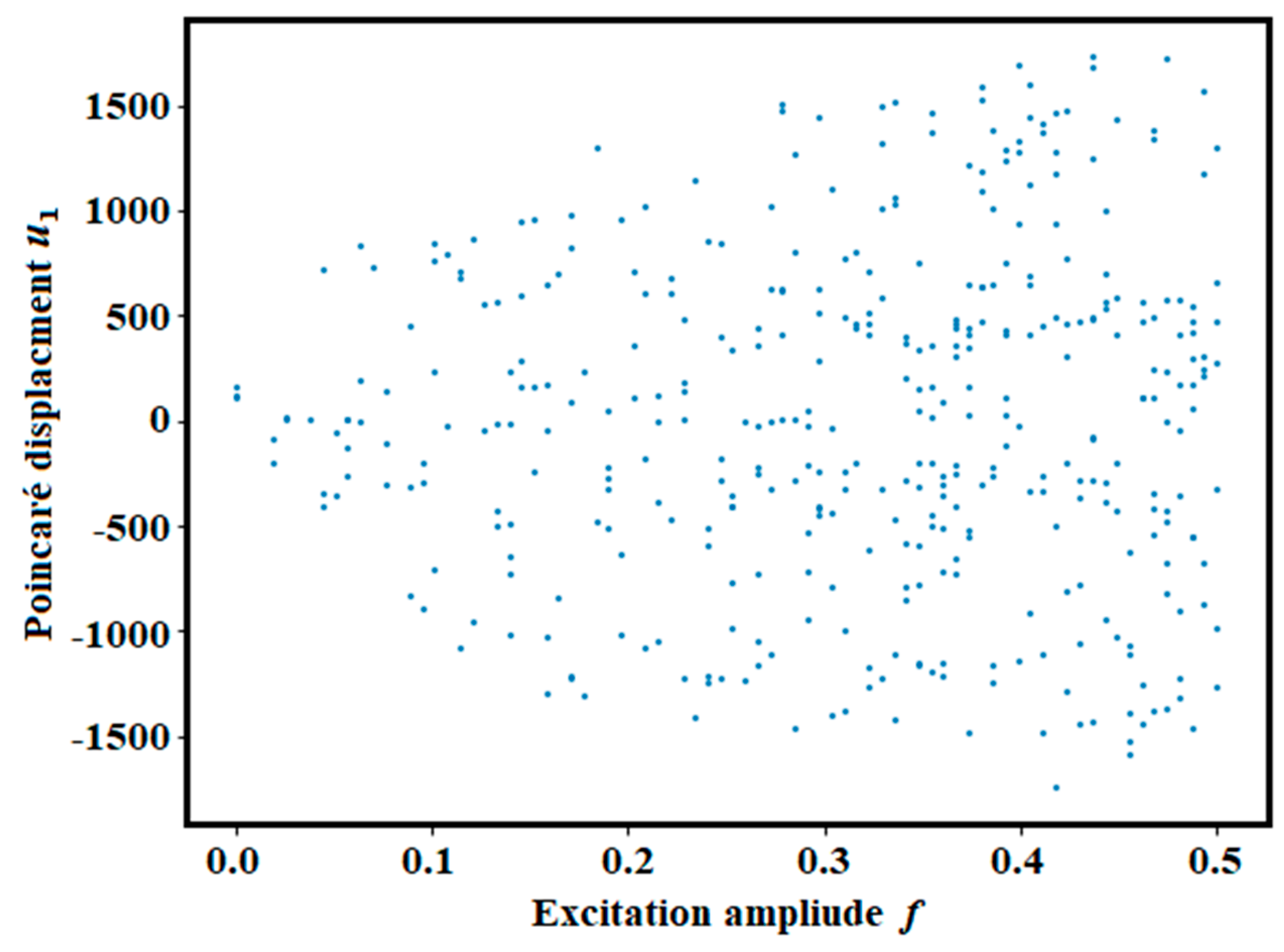
As the excitation amplitude $f$ increases, the Poincaré points of $u_1$ evolve from single points to multiple branches and finally to dense clouds, as seen in Figure 20. At low $f$, the forcing is weak, the NES is barely activated, and the response remains nearly linear and period-1, with most energy staying in the primary oscillator.

Figure 20. Shows a bifurcation plot via $f$.

At intermediate excitation levels ($f\approx$ 0.15–0.3) introduce significant nonlinear stiffness, leading to internal resonance between the main oscillator and the NES. In this range, the system begins to exhibit period-doubling and quasiperiodic responses. Physically, this regime is associated with enhanced interaction between the primary oscillator and the NES, where nonlinear coupling facilitates increased energy exchange. At high excitation amplitudes ($f\ge 0.3$), the response collapses into dense clouds, indicating chaotic dynamics driven by nonlinear interactions. The NES then absorbs energy through irregular, chaotic modulation rather than smooth periodic transfer. Thus, increasing the excitation amplitude progressively activates the NES, initiating resonance capture, driving bifurcations, and ultimately leading to chaotic TET.

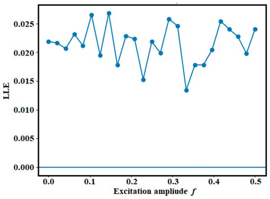
The LLE is computed for excitation amplitudes $f\in [0,0.5]$, as shown in Figure 21. Since negative, zero, and positive LLE values correspond to periodic, quasiperiodic, and chaotic behavior, respectively, the predominantly positive LLE values indicate widespread chaotic dynamics. As $f$ increases, the LLE also grows, reflecting enhanced sensitivity to initial conditions due to nonlinear energy exchange between the oscillator and the NES. This growth signals intensified modal interactions and increasing irregularity, characteristic of chaotic TET.

Figure 21. Displays LLE via excitation amplitude $f$.

Consequently, the NES does not merely reduce vibration through periodic motion; rather, it dissipates energy via chaotic and irreversible exchange, as evidenced by the positive Lyapunov exponents.

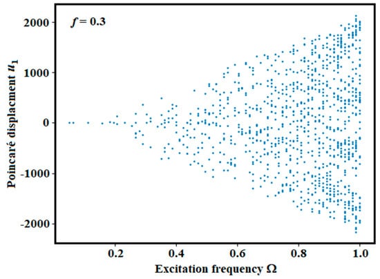
The bifurcation diagram with respect to excitation frequency $\Omega \in [0.05,1.0],f=0$ is shown in Figure 22. It reveals small oscillation amplitudes at low $\Omega$, branch splitting near resonance, and dense chaotic point clouds as $\Omega$ approaches 1. At low frequencies ($\Omega \le 0.25$), the system behaves nearly linearly with small oscillations, as it is far from resonance and the NES remains weakly excited. For intermediate frequencies ($0.25\le \Omega \le 0.55$), internal resonance develops, enabling energy transfer to the NES and leading to repeated capture–release interactions characteristic of nonlinear modal coupling. At higher frequencies ($0.55\le \Omega \le 0.9$), the response becomes chaotic, producing dense point clouds and nonlinear energy pumping from the primary oscillator to the NES. Near resonance ($\Omega \to 1$), the system exhibits large dispersion alongside chaotic oscillations. Physically, this reflects the resonant excitation of the NES, which induces intermittent energy pumping and chaotic energy flow, indicating that the absorber is fully engaged.

Figure 22. Presents a bifurcation diagram versus $\Omega$ at f = 0.3.

As a consequence, tuning the excitation frequency governs the activation of the NES and the transition from periodic to chaotic energy transfer. The bifurcation and Lyapunov analyses show that increasing either the excitation amplitude or frequency activates the NES through internal resonance. At low forcing, the motion remains periodic; at moderate levels, resonance capture initiates TET; and at higher levels, successive bifurcations lead to chaotic regimes with positive Lyapunov exponents, indicating irreversible and highly sensitive energy exchange. These results demonstrate that vibration mitigation is primarily achieved through chaotic TET rather than periodic absorption.

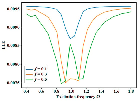
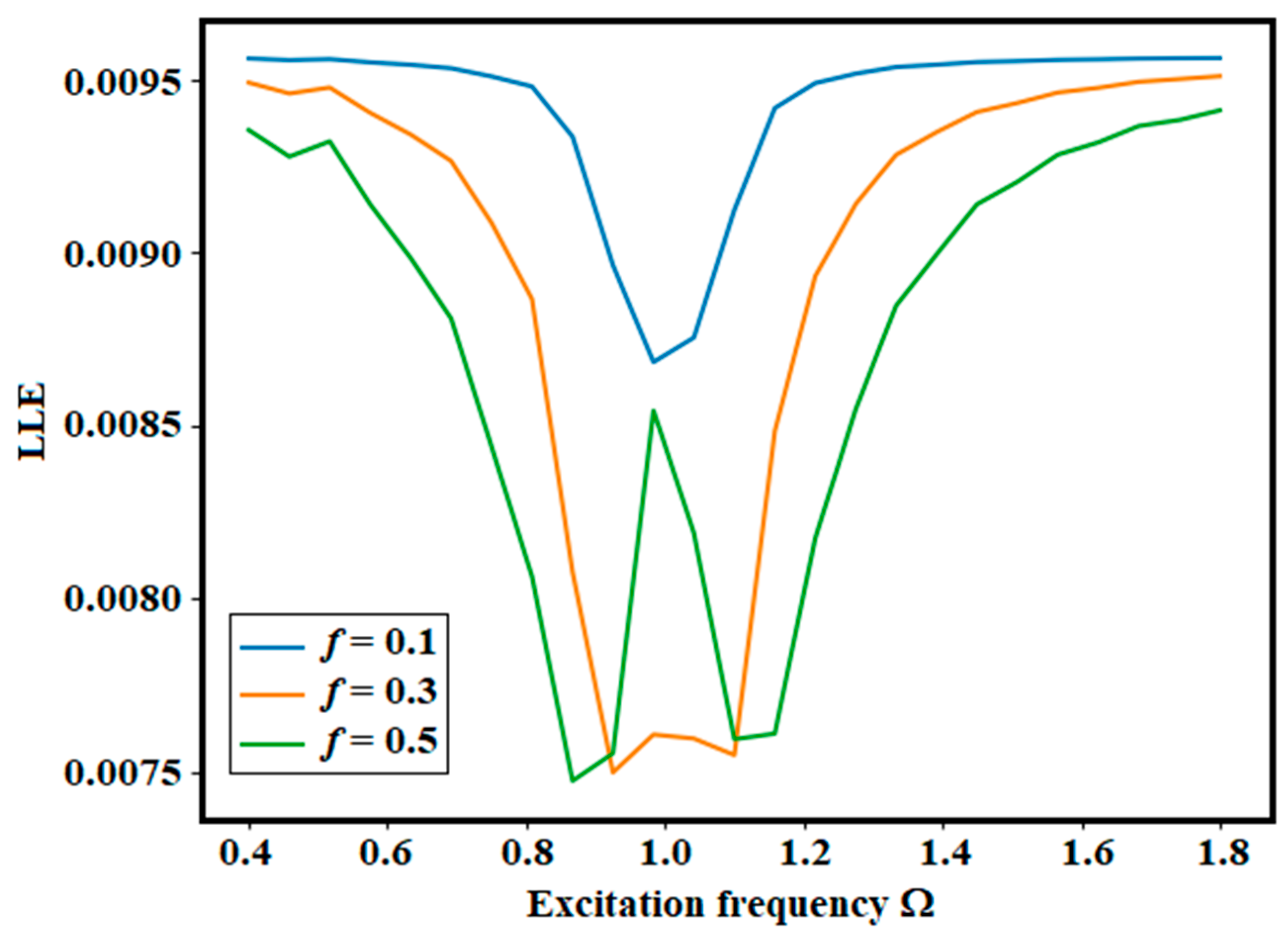
The LLE as a function of excitation frequency $\Omega$ was evaluated for three excitation amplitudes: $f=(0.1,0.3,0.5)$, as demonstrated in Figure 23. This figure presents the three LLE curves plotted together. As previously noted, positive LLE values indicate chaotic or irregular motion, negative values correspond to stable periodic responses, and values near zero represent quasi-periodic transitions. In this case, the LLE values remain small and positive, signifying weak chaos or complex modulated oscillations in the vicinity of the resonance region.

Figure 23. Shows LLE versus $\Omega$ for different excitation amplitudes.

We now examine how the excitation frequency $\Omega$ influences the system’s behavior. All three curves show a noticeable dip around $\Omega \approx 1$, corresponding to the primary resonance zone. In this region, energy exchange between the main oscillator and the system strengthens, nonlinear interactions reduce exponential divergence, and the motion becomes more organized. This indicates that the NES operates most effectively near resonance.

The role of the excitation amplitude $f$ can be summarized as follows: as f increases from 0.1 to 0.3 and 0.5, the system exhibits lower LLE values near resonance, nonlinear energy pumping, more pronounced modulation, and greater sensitivity away from resonance. The dip in the LLE curve indicates that the NES suppresses chaotic divergence by absorbing energy from the primary system near $\Omega \approx 1$.

8. Concluding Insights

This study investigated the nonlinear dynamics of a harmonically forced primary oscillator coupled to a 2DOF-NES. The analysis focused on the role of nonlinear coupling in shaping energy redistribution and stability characteristics of the system under varying excitation and parameter conditions. The governing dynamics were examined using the proposed NPA, and the results were validated through direct NSs. The comparison between analytical predictions and NSs demonstrated good agreement across different operating regimes, confirming the capability of the proposed formulation to capture the essential nonlinear response behavior of the coupled system. The stability analysis showed that the system response is influenced by the cubic coupling strength, as well as the damping and stiffness parameters of the NES, which collectively govern the onset of instability and the persistence of bounded oscillations. The main findings of this work may be summarized as follows:

• The coupled primary oscillator–2DOF-NES can be effectively represented through an equivalent amplitude-dependent formulation derived from the NPA framework.
• The analytical predictions show good consistency with direct NSs over a range of parameter variations.
• The system exhibits sustained periodic responses in significant parameter regions, confirming the effectiveness of nonlinear coupling in maintaining bounded dynamics.
• Stability is mainly governed by the nonlinear coupling strength and NES parameters, which significantly influence the transition between stable/unstable regimes.

Future Work

Future work will focus on extending the proposed framework to nonlinear systems with more complex coupling configurations and additional physical effects, including time delay, stochastic excitation, and parameter uncertainty. A more detailed energy-flow analysis, including instantaneous and cumulative energy evolution of the coupled components, represents a possible extension to further investigate the physical interpretation of the system dynamics. In addition, systematic benchmarking against established analytical and numerical techniques, such as the Harmonic Balance Method, Multiple Scales, Averaging Method, and continuation-based tools (e.g., AUTO and MATCONT), as well as robustness-oriented studies using Monte Carlo simulation and sensitivity analysis, may be considered in future investigations to further assess the performance of the proposed formulation. Experimental validation is also identified as a potential direction for supporting the theoretical and numerical findings and enhancing the applicability of the model in practical engineering systems.

References

- Kang, X.; Tang, J.; Xia, G.; Wei, J.; Zhang, F.; Sheng, Z. Design, optimization and application of nonlinear energy sink in energy harvesting device. Int. J. Energy Res. 2024, 2024, 2811428. [Google Scholar] [CrossRef] [Scilit]
- Gendelman, O.V.; Bar, T. Bifurcations of self-excitation regimes in a van der Pol oscillator with a nonlinear energy sink. Phys. D. 2010, 239, 220–229. [Google Scholar] [CrossRef] [Scilit]
- Starosvetsky, Y.; Gendelman, O.V. Vibration absorption in systems with a nonlinear energy sink: Nonlinear damping. J. Sound. Vib. 2009, 324, 916–939. [Google Scholar] [CrossRef] [Scilit]
- Gendelman, O.V.; Starosvetsky, Y.; Feldman, M. Attractors of harmonically forced linear oscillator with attached nonlinear energy sink I: Description of response regimes. Nonlinear Dyn. 2008, 51, 31–46. [Google Scholar] [CrossRef] [Scilit]
- Starosvetsky, Y.; Gendelman, O.V. Attractors of harmonically forced linear oscillator with attached nonlinear energy sink II: Optimization of a nonlinear vibration absorber. Nonlinear Dyn. 2008, 51, 47–57. [Google Scholar] [CrossRef] [Scilit]
- Vakakis, A.F. Inducing passive nonlinear energy sinks in linear vibrating systems. J. Vib. Acoust. 2001, 123, 324–332. [Google Scholar] [CrossRef] [Scilit]
- Taghipour, J.; Dardel, M. Steady-state dynamics and robustness of a harmonically excited essentially nonlinear oscillator coupled with a two-DOF nonlinear energy sink. Mech. Syst. Signal Process. 2015, 62–63, 164–182. [Google Scholar] [CrossRef] [Scilit]
- Kerschen, G.; Worden, K.; Vakakis, A.F.; Golinval, J.C. Past, present and future of nonlinear system identification in structural dynamics. Mech. Syst. Signal Process. 2006, 20, 505–592. [Google Scholar] [CrossRef] [Scilit]
- Cao, M.S.; Sha, G.G.; Gao, Y.F.; Ostachowicz, W. Structural damage identification using damping: A compendium of uses and features. Smart Mater. Struct. 2017, 26, 043001. [Google Scholar] [CrossRef] [Scilit]
- Blackwell, C.; Palazotto, A.; George, T.J.; Cross, C.J. The evaluation of the damping characteristics of a hard coating on titanium. Shock. Vib. 2007, 14, 37–51. [Google Scholar]
- Liang, J.W.; Feeny, B.F. Identifying Coulomb and viscous friction in forced dual-damped oscillators. J. Vib. Acoust. 2004, 126, 118–125. [Google Scholar] [CrossRef] [Scilit]
- Mevada, H.; Patel, D. Experimental determination of structural damping of different materials. Process Eng. 2016, 144, 110–115. [Google Scholar] [CrossRef] [Scilit]
- Zhang, X.; Du, X.; Brownjohn, J. Frequency modulated empirical mode decomposition method for the identification of instantaneous modal parameters of aero elastic systems. J. Wind Eng. Ind. Aerodyn. 2012, 101, 43–52. [Google Scholar] [CrossRef] [Scilit]
- Kulkarni, P.; Bhattacharjee, A.; Nanda, B.K. Study of damping in composite beams. Mater. Today Proc. 2018, 5, 7061–7067. [Google Scholar] [CrossRef] [Scilit]
- Chatterjee, A.; Chintha, H.P. Identification and parameter estimation of cubic nonlinear damping using harmonic probing and Volterra series. Int. J. Non-Linear Mech. 2020, 125, 103518. [Google Scholar] [CrossRef] [Scilit]
- Dou, C.; Fan, J.; Li, C.; Cao, J.; Gao, M. On discontinuous dynamics of a class of friction-influenced oscillators with nonlinear damping under bilateral rigid constraints. Mech. Mach. Theory 2020, 147, 103750. [Google Scholar] [CrossRef] [Scilit]
- Barakat, A.A.; Weig, E.M.; Hagedorn, P. Non-trivial solutions and their stability in a two-degree-of-freedom Mathieu–Duffing system. Nonlinear Dyn. 2023, 111, 22119–22136. [Google Scholar] [CrossRef] [Scilit]
- He, J.-H. Comment on He’s frequency formulation for nonlinear oscillators. Int. J. Nonlinear Sci. Numer. Simul. 2008, 29, 19–22. [Google Scholar] [CrossRef] [Scilit]
- He, J.-H. An approximate amplitude-frequency relationship for a nonlinear oscillator with discontinuity. Nonlinear Sci. Lett. A 2016, 7, 77–85. [Google Scholar]
- He, J.-H. Amplitude-frequency relationship for conservative nonlinear oscillators with odd nonlinearities. Int. J. Appl. Comput. Math. 2017, 3, 1557–1560. [Google Scholar] [CrossRef] [Scilit]
- Ren, Z.F. He’s frequency-amplitude formulation for nonlinear oscillators. Int. J. Mod. Phys. B 2011, 25, 2379–2382. [Google Scholar] [CrossRef] [Scilit]
- Ren, Z. Theoretical basis of He’s frequency-amplitude formulation for nonlinear oscillators. Nonlinear Sci. Lett. A 2018, 9, 86–90. [Google Scholar]
- García, A. An amplitude-period formula for a second order nonlinear oscillator. Nonlinear Sci. Lett. A 2017, 8, 340–347. [Google Scholar]
- Antola, R.S. Remarks on an approximate formula for the period of conservative oscillations in nonlinear second order ordinary differential equations. Nonlinear Sci. Lett. A 2017, 8, 348–351. [Google Scholar]
- Younesian, D.; Askari, H.; Saadatnia, Z.; Yazdi, M.K. Frequency analysis of strongly nonlinear generalized Duffing oscillators using He’s frequency–amplitude formulation and He’s energy balance method. Comput. Math. Appl. 2010, 59, 3222–3228. [Google Scholar] [CrossRef] [Scilit]
- Ren, Z.-F.; Hu, G.-F. He’s frequency–amplitude formulation with average residuals for nonlinear oscillators. J. Low. Freq. Noise Vib. Act. Control 2019, 38, 1050–1059. [Google Scholar] [CrossRef] [Scilit]
- Almutlg, A.; Moatimid, G.M.; Amer, T.S.; Mohamed, Y.M. Non-perturbative analysis of bifurcation and chaotic dynamics of a cantilever beam under triple time-delayed feedback control. AIMS Math. 2026, 11, 17492–17527. [Google Scholar] [CrossRef] [Scilit]
- Moatimid, G.M.; Mohamed, Y.M. An innovative methodology in scrutinizing the nonlinear stability of two immiscible MHD viscoelastic liquids. Math. Comput. Simul. 2025, 234, 472–496. [Google Scholar] [CrossRef] [Scilit]
- Almutlg, A.; Moatimid, G.M.; Amer, T.S.; Mohamed, Y.M. Nonlinear analysis of periodic/quasi-periodic dynamics of a forced Duffing oscillator using the non-perturbative approach. J. Math. 2026. accepted for publication. [Google Scholar]
- Moatimid, G.M.; Mohamed, Y.M. Advanced analysis of nonlinear stability of two horizontal interfaces separating three stratified non-Newtonian liquids. Sci. Rep. 2025, 15, 40396. [Google Scholar] [CrossRef] [Scilit] [PubMed]
- Zavodney, L.D.; Nayfeh, A.H. The non-linear response of a slender beam carrying a lumped mass to a principal parametric excitation: Theory and experiment. Int. J. Non-Linear Mech. 1989, 24, 105–125. [Google Scholar] [CrossRef] [Scilit]
- Nayfeh, A.H.; Balachandran, B. Applied Nonlinear Dynamics: Analytical, Computational, and Experimental Methods; John Wiley & Sons: New York, NY, USA, 1995. [Google Scholar] [CrossRef] [Scilit]
- El-Dib, Y.O. Insightful and comprehensive formularization of frequency–amplitude formula for strong or singular nonlinear oscillators. J. Low. Freq. Noise Vib. Act. Control 2023, 42, 89–109. [Google Scholar] [CrossRef] [Scilit]
- El-Dib, Y.O. A review of the frequency-amplitude formula for nonlinear oscillators and its advancements. J. Low. Freq. Noise Vib. Act. Control 2024, 43, 1032–1064. [Google Scholar] [CrossRef] [Scilit]
- El-Dib, Y.O. The masking technique for forced nonlinear oscillator stability behavior analysis using the non-perturbative approach. J. Low. Freq. Noise Vib. Act. Control 2024, 43, 1481–1497. [Google Scholar] [CrossRef] [Scilit]
- Sidorov, N.; Sidorov, D.; Li, Y. Basins of attraction and stability of nonlinear systems’ equilibrium points. Differ. Equ. Dyn. Syst. 2023, 31, 289–300. [Google Scholar] [CrossRef] [Scilit]
- Taborda, J.A.; Angulo, F. Computing and controlling basins of attraction in multistability scenarios. Math. Probl. Eng. 2015, 2015, 313154. [Google Scholar] [CrossRef] [Scilit]
- Abohamer, M.K.; Amer, T.S.; Abdelhfeez, S.A.; Eldawoody, D.A.; Elbaz, R.F. Vibration analysis, stability assessment, and chaotic behavior of a damped oscillator coupled with a spherical pendulum and a piezoelectric transducer. Nonlinear Dyn. 2025, 113, 24343–24381. [Google Scholar] [CrossRef] [Scilit]
- Benettin, G.; Galgani, L.; Giorgilli, A.; Strelcyn, J.M. Lyapunov characteristic exponents for smooth dynamical systems and for Hamiltonian systems: A method for computing all of them. Part 1: Theory. Meccanica 1980, 15, 9–20. [Google Scholar] [CrossRef] [Scilit]
Disclaimer/Publisher’s Note: The statements, opinions and data contained in all publications are solely those of the individual author(s) and contributor(s) and not of MDPI and/or the editor(s). MDPI and/or the editor(s) disclaim responsibility for any injury to people or property resulting from any ideas, methods, instructions or products referred to in the content. |
© 2026 by the authors. Licensee MDPI, Basel, Switzerland. This article is an open access article distributed under the terms and conditions of the Creative Commons Attribution (CC BY) license.