Stability, Bifurcation Analysis and Chaos in a Discretized Fractional-Order Predator–Prey System with Nonlinear Functional Response

Abstract

This study examines a discrete fractional-order predator–prey system incorporating a Holling type-III functional response. The Caputo fractional derivative is employed because it naturally incorporates memory and hereditary effects while preserving biologically meaningful initial conditions. The system is formulated from a biologically relevant continuous fractional-order framework through the application of the piecewise constant argument approach, enabling an analysis of how memory-dependent effects and discrete dynamics influence predator–prey interactions. The existence and local stability of fixed points are determined by using the Jacobian matrix and eigenvalue conditions. The bifurcation of the positive fixed point is analyzed by using the center manifold and normal form methods. Numerical simulations, including bifurcation diagrams, phase portraits, and maximum Lyapunov exponent plots, confirm our analytical results and reveal periodic, quasiperiodic, and chaotic behavior. The findings of this study reveal that the combined influence of memory-dependent dynamics, nonlinear predator–prey interactions, and discrete-time effects can generate rich and complicated behaviors in fractional-order predator-prey systems.

1. Introduction

Predator–prey interactions represent one of the central concepts in population ecology and have been widely studied to better understand the mechanisms that govern species coexistence, population regulation, and the overall stability of ecological systems. From the early models by Lotka and Volterra [1,2], mathematical modeling of predator–prey dynamics has become increasingly sophisticated and now also includes nonlinear functional responses [3,4], Allee effects [5,6], harvesting [7], slow–fast effects [8], refuge [9], and fear effects [10]. So far, such modeling has shown that relatively simple rules of interaction can produce a broad range of dynamical behaviors, like stable equilibria, population cycles, quasiperiodicity, and chaos. To some extent, these behaviors are interesting not only from a theoretical perspective but also from practical viewpoints related to biodiversity conservation, biological control, and sustainable ecosystem management.

Traditionally, predator–prey dynamics have been modeled by systems of ordinary differential equations, which implicitly assume that population growth and interactions depend only on the current state of the system. However, many real ecological processes are characterized by memory and hereditary effects. Indeed, biological factors in predator learning, prey refuge utilization, gestation periods, maturation delays, and accumulated environmental stress seem to point toward the fact that the present population dynamics may be adequately represented depending not on instantaneous densities, but rather on population sizes from the past. Inherently, classical integer-order models cannot account for such kinds of nonlocal temporal effects. Moreover, with regard to nonlocal temporal effects, fractional-order differential equations, which are far more flexible than their integer-order counterparts, have become an increasingly powerful modeling framework in population dynamics, as in many other areas of science. Fractional derivatives, in particular in the Caputo sense, naturally incorporate memory effects through power-law weighting of past states, which allows current dynamics to reflect the cumulative influence of historical population interactions.

In recent years, fractional-order predator–prey models have attracted considerable attention due to their ability to reproduce more realistic ecological dynamics than their integer-order counterparts. It was demonstrated that incorporation of fractional derivatives can affect stability regions, delay oscillation onset, and move bifurcation points. The fractional order is an additional parameter that varies between memoryless and memory-rich behavior. From an ecological point of view, this parameter can represent the strength of long-term biological memory or environment persistence in a meaningful extension of traditional predator–prey models.

Recently, a number of studies have been conducted on various fractional order predator–prey models with different ecological interactions. Li et al. [11] proposed a fractional-order predator–prey model with prey refuge and proved the existence, uniqueness, non-negativity, and boundedness of the solutions and the global stability analysis of predator extinction and coexistence equilibrium. Suryanto et al. [12] studied a fractional-order predator–prey model with a ratio-dependent functional response and linear harvesting, and they established the stability criteria of the model by utilizing Matignon’s theorem and Lyapunov functions, and they also showed the occurrence of Hopf bifurcation analytically. Djilali and Ghanbari [13] examined a fractional-order eco-epidemiological predator–prey model including a non-fatal infectious disease in the prey population and cooperative hunting in the predator population, and they showed that the fractional order enriched the dynamics of the model and had a significant effect on stability properties. Hariprasad et al. [14] developed a fractional-order prey-predator-disease model with Holling-type functional responses and demonstrated that variations in the fractional order could induce transitions from chaotic to stable dynamics. More recently, Wei et al. [15] analyzed stability, bifurcation, and control in a fractional-order predator–prey system with time delay, revealing the combined effects of fractional order and delay on bifurcation behavior and showing that feedback control could suppress undesirable dynamics.

Another important issue in predator–prey modeling is the choice of functional response. It explains how the rate of predation depends on prey density. Holling [16] proposed three classical types of functional responses that are linear (type I), hyperbolic (type II), and sigmoidal (type III). The linear type I response, as given by $f\left(x\right)=ax$, signifies a proportional relationship between prey density and consumption rate. The type II response, $f\left(x\right)={\displaystyle \frac{ax}{1+ahx}}$, takes into account the handling time of the predator and as a result, saturation occurs at high prey densities. The sigmoidal type III response, $f\left(x\right)={\displaystyle \frac{a{x}^p}{1+ah{x}^p}}$, $p>1$, reflects predator learning and prey switching behavior, resulting in reduced predation at low prey densities. Holling type III functional response is particularly pertinent in ecosystems where a certain threshold prey density can initiate hunting for the predators, which is commonly observed in insectivorous and vertebrate predators. Extensions and generalizations of these functional responses have been proposed by Beddington and DeAngelis [17,18], Crowley and Martin [19] and many subsequent studies [20,21,22,23,24].

From an ecological perspective, fractional-order derivatives offer a natural framework for the inclusion of memory and hereditary properties of biological systems, where the current state is affected by past dynamics. For example, predator dynamics could be affected by past hunting experiences and learning processes, while prey populations could be affected by delayed environmental responses or the cumulative effects of resource availability. Such dependencies cannot be modeled in a satisfactory manner using traditional integer-order models. In addition, many ecological processes are naturally discrete in time because of factors such as seasonal breeding patterns, migration patterns, or periodic harvesting, making discrete-time models more suitable in such cases. Therefore, the combination of fractional-order memory with discrete dynamics offers a versatile framework for modeling systems that exhibit both temporal delays and seasonal variations, such as insect populations, plankton dynamics, and predator–prey dynamics under periodic environmental conditions.

Even though continuous models can offer important insights, there exist many discrete phenomena in nature. Ecological data, for instance, tend to be discretely measured in units of seasons or generations, and biological activities like reproduction or harvesting tend to happen in pulses rather than continuously in time. The numerical simulation of continuous models in time usually requires discretization, and this process, far from being just a practical necessity, can change the qualitative features of the original model. Discrete-time predator–prey models have more complex behavior than their continuous-time counterparts, who exhibit period-doubling cascades, Neimark–Sacker bifurcations, and chaotic behavior even when their respective continuous models are stable [25,26,27,28].

In the context of fractional order systems, the discretization process adds an extra degree of complexity by merging the concept of memory with the concept of discrete time evolution. Various techniques have been proposed for the discretization of fractional differential equations. Among these, the piecewise constant argument method [29,30,31] has been particularly successful. This technique preserves the qualitative properties of the original fractional order system while ensuring that the resulting discrete time evolution is more tractable from an analytical viewpoint. Moreover, the resulting discrete time model includes the fractional order in the form of the time step.

Consequently, discretized fractional-order predator–prey models have attracted growing attention in recent years. Elsadany and Matouk [32] showed that a discretized fractional-order Lotka–Volterra system exhibited transcritical, flip, and NS bifurcations and chaos, even though the continuous fractional-order model admitted only stable or unstable equilibria. Singh et al. [33] analyzed a discrete fractional-order Leslie–Gower predator–prey model and demonstrated that variations in the fractional order and step size could generate flip and NS bifurcations, quasiperiodicity, and chaotic dynamics. Mondal et al. [34] studied a fractional-order predator–prey system with habitat complexity and its discretized counterpart, showing that the discrete model exhibited richer dynamics strongly dependent on both fractional order and step size. Panigoro et al. [35] and Uddin and Podder [36] further demonstrated that discretized fractional-order ecological models can exhibit complex bifurcation structures and chaos, which can be effectively controlled using suitable strategies.

Motivated by these studies, the present work focuses on a discretized fractional-order predator–prey model with Holling type III functional response. To the best of our knowledge, a detailed bifurcation analysis of a discretized fractional-order predator–prey model with Holling type III functional response obtained via the piecewise constant argument approach has not been reported previously. We begin with a biologically meaningful fractional-order continuous-time model describing the interaction between prey and predator populations, where the prey grows logistically and is consumed by predators according to a Holling type III functional response, while predator growth depends on the conversion of consumed prey biomass.

Definition 1

([37]). The Caputo fractional derivative of order σ for a function $f\in C^n([t_0,\infty ),\mathbb{R})$ is defined as

$$\begin{array}{c}\hfill {}^C\mathrm{D}_{t_0}^{\sigma }f\left(t\right)={\displaystyle \frac{1}{\Gamma (n-\sigma )}}{\int }_{t_0}^t{(t-\tau )}^{n-\sigma -1}{f}^{\left(n\right)}\left(\tau \right)\mathrm{d}\tau ,\end{array}$$

(1)

where $\Gamma \left(n\right)$ denotes the classical Gamma function, $t\ge t_0$, and $n\in \mathbb{N}$ such that $n-1<\sigma <n$. In particular, when $0<\sigma <1$, then

$$\begin{array}{c}\hfill {}^C\mathrm{D}_{t_0}^{\sigma }f\left(t\right)={\displaystyle \frac{1}{\Gamma (1-\sigma )}}{\int }_{t_0}^t{(t-\tau )}^{-\sigma }{f}^{\prime }\left(\tau \right)\mathrm{d}\tau .\end{array}$$

(2)

Using the Caputo fractional derivative, we consider the following fractional-order predator–prey model with Holling type III functional response [38]:

$$\left\{\begin{array}{c}{\displaystyle \frac{{\mathrm{d}}^{\sigma }x}{\mathrm{d}{t}^{\sigma }}}=\alpha x-{\displaystyle \frac{\beta x^{2}y}{x^2+\eta }},\hfill \\ {\displaystyle \frac{{\mathrm{d}}^{\sigma }y}{\mathrm{d}{t}^{\sigma }}}=-\gamma y+{\displaystyle \frac{\delta x^{2}y}{x^2+\eta }},\hfill \end{array}\right.$$

(3)

where $x\left(t\right)$ and $y\left(t\right)$ denote the prey and predator population densities, respectively. The parameter $\sigma \in (0,1]$ represents the fractional order and captures the memory effect in the system, with smaller values corresponding to stronger memory. The proposed framework describes a predator–prey interaction in which the prey population follows logistic growth with intrinsic growth rate $\alpha$. The predation process is represented by a Holling type III function and is given by ${\displaystyle \frac{\beta x^{2}y}{x^2+\eta }}$, where $\beta$ is a predation coefficient. The value of $\eta$ is a half-saturation constant, which regulates the transition from a weak to a strong predation process and takes into account different processes such as the adaptation of predators and weakening of the predation process with a decrease in the density of the prey population. The growth of the predator population is supported by the consumption of the prey with a conversion efficiency $\delta$, which characterizes the rate of conversion of consumed biomass into growth. Moreover, by using a Caputo fractional derivative, it is possible to include memory effects into the model, and it should be noted that the evolution of such a model depends not only on the current populations but also on their past values. Furthermore, the Caputo derivative allows for the use of biologically meaningful initial conditions expressed directly in terms of population densities, making it particularly suitable for ecological modeling.

To derive the discrete analogue of (3), we apply the piecewise constant argument technique. Following the procedure of Mondal et al. [34], we rewrite (3) by freezing the state variables on each time interval of length $h>0$ as follows:

$$\begin{array}{cc}\hfill {}_0{}^{C}D_t^{\sigma }x\left(t\right)& =\alpha x\left([t/h]h\right)-{\displaystyle \frac{\beta x^2\left([t/h]h\right)y\left([t/h]h\right)}{x^2\left([t/h]h\right)+\eta }},\hfill \\ \hfill {}_0{}^{C}D_t^{\sigma }y\left(t\right)& =-\gamma y\left([t/h]h\right)+{\displaystyle \frac{\delta x^2\left([t/h]h\right)y\left([t/h]h\right)}{x^2\left([t/h]h\right)+\eta }},\hfill \end{array}$$

(4)

with initial condition $x\left(0\right)=x_0>0$, $y\left(0\right)=y_0>0$.

Let $t\in [0,h)$ so that $t/h\in [0,1)$. Then $[t/h]=0$ and (4) becomes

$${}_0{}^{C}D_t^{\sigma }x\left(t\right)=\alpha x_0-{\displaystyle \frac{\beta x_0^2{y}_0}{x_0^2+\eta }},{}_0{}^{C}D_t^{\sigma }y\left(t\right)=-\gamma y_0+{\displaystyle \frac{\delta x_0^2{y}_0}{x_0^2+\eta }}.$$

Hence, the solution on $[0,h)$ can be written in the integral form as

$$x_1\left(t\right)=x_0+J_0^{\sigma }\left(\alpha x_0-{\displaystyle \frac{\beta x_0^2{y}_0}{x_0^2+\eta }}\right)=x_0+{\displaystyle \frac{t^{\sigma }}{\Gamma (\sigma +1)}}\left(\alpha x_0-{\displaystyle \frac{\beta x_0^2{y}_0}{x_0^2+\eta }}\right),$$

$$y_1\left(t\right)=y_0+J_0^{\sigma }\left(-\gamma y_0+{\displaystyle \frac{\delta x_0^2{y}_0}{x_0^2+\eta }}\right)=y_0+{\displaystyle \frac{t^{\sigma }}{\Gamma (\sigma +1)}}\left(-\gamma y_0+{\displaystyle \frac{\delta x_0^2{y}_0}{x_0^2+\eta }}\right),$$

where

$$J_0^{\sigma }f\left(t\right)={\displaystyle \frac{1}{\Gamma \left(\sigma \right)}}{\int }_0^t{(t-\tau )}^{\sigma -1}f\left(\tau \right)d\tau ,\sigma >0,$$

Next, assume $t\in [h,2h)$ so that $t/h\in [1,2)$ and $[t/h]=1$. Then (4) gives

$${}_0{}^{C}D_t^{\sigma }x\left(t\right)=\alpha x_1\left(h\right)-{\displaystyle \frac{\beta x_1^2\left(h\right)y_1\left(h\right)}{x_1^2\left(h\right)+\eta }},{}_0{}^{C}D_t^{\sigma }y\left(t\right)=-\gamma y_1\left(h\right)+{\displaystyle \frac{\delta x_1^2\left(h\right)y_1\left(h\right)}{x_1^2\left(h\right)+\eta }}.$$

Thus, the solution on $[h,2h)$ reads

$$x_2\left(t\right)=x_1\left(h\right)+J_h^{\sigma }\left(\alpha x_1\left(h\right)-{\displaystyle \frac{\beta x_1^2\left(h\right)y_1\left(h\right)}{x_1^2\left(h\right)+\eta }}\right)=x_1\left(h\right)+{\displaystyle \frac{{(t-h)}^{\sigma }}{\Gamma (\sigma +1)}}\left(\alpha x_1\left(h\right)-{\displaystyle \frac{\beta x_1^2\left(h\right)y_1\left(h\right)}{x_1^2\left(h\right)+\eta }}\right),$$

$$y_2\left(t\right)=y_1\left(h\right)+J_h^{\sigma }\left(-\gamma y_1\left(h\right)+{\displaystyle \frac{\delta x_1^2\left(h\right)y_1\left(h\right)}{x_1^2\left(h\right)+\eta }}\right)=y_1\left(h\right)+{\displaystyle \frac{{(t-h)}^{\sigma }}{\Gamma (\sigma +1)}}\left(-\gamma y_1\left(h\right)+{\displaystyle \frac{\delta x_1^2\left(h\right)y_1\left(h\right)}{x_1^2\left(h\right)+\eta }}\right),$$

where

$$J_h^{\sigma }f\left(t\right)={\displaystyle \frac{1}{\Gamma \left(\sigma \right)}}{\int }_h^t{(t-\tau )}^{\sigma -1}f\left(\tau \right)d\tau ,\sigma >0.$$

Repeating this process, for $t\in [nh,(n+1\left)h\right)$ we obtain

$$x_{n+1}\left(t\right)=x_n\left(nh\right)+{\displaystyle \frac{{(t-nh)}^{\sigma }}{\Gamma (\sigma +1)}}\left(\alpha x_n\left(nh\right)-{\displaystyle \frac{\beta x_n^2\left(nh\right)y_n\left(nh\right)}{x_n^2\left(nh\right)+\eta }}\right),$$

$$y_{n+1}\left(t\right)=y_n\left(nh\right)+{\displaystyle \frac{{(t-nh)}^{\sigma }}{\Gamma (\sigma +1)}}\left(-\gamma y_n\left(nh\right)+{\displaystyle \frac{\delta x_n^2\left(nh\right)y_n\left(nh\right)}{x_n^2\left(nh\right)+\eta }}\right).$$

Letting $t\to (n+1)h$ and denoting $x_n=x\left(nh\right)$, $y_n=y\left(nh\right)$, we arrive at the discrete fractional-order model

$$\left\{\begin{array}{c}{x}_{n+1}=x_n+\tau \left(\alpha x_n-{\displaystyle \frac{\beta x_n^2{y}_n}{x_n^2+\eta }}\right),\hfill \\ y_{n+1}=y_n+\tau \left(-\gamma y_n+{\displaystyle \frac{\delta x_n^2{y}_n}{x_n^2+\eta }}\right),\hfill \end{array}\right.$$

(5)

where $\tau ={\displaystyle \frac{h^{\sigma }}{\Gamma (\sigma +1)}}$. For analytical convenience, the quantity $\tau$ is introduced to simplify the stability and bifurcation calculations. Nevertheless, the fractional order $\sigma$ remains an inherent component of the discrete-time model (5) through its explicit appearance in $\tau$. Consequently, variations in $\sigma$ directly affect the system dynamics. This influence is further demonstrated in the numerical section, where $\sigma$ is treated as a bifurcation parameter and changes in its value are shown to induce qualitative transitions in the dynamics, including the occurrence of PD and NS bifurcations and chaotic behavior.

Biologically, the discrete formulation is suitable for populations evolving through distinct periods such as generations, breeding seasons, or harvesting cycles. In the discrete system, each iteration represents the population state from one period to the next. Furthermore, $\tau ={\displaystyle \frac{h^{\sigma }}{\Gamma (\sigma +1)}}$ captures the combined effects of the observation interval and the fractional order, thereby reflecting how temporal scale and memory jointly influence the predator–prey dynamics.

It is important to mention that the reason for choosing the piecewise constant argument method in this work is its efficiency in the qualitative analysis of dynamical systems. In contrast to the standard numerical methods for solving fractional differential equations, like the Adams–Bashforth–Moulton predictor-corrector method, which are mainly used for precise numerical solutions and involve convolution terms for memory computations, the piecewise constant argument method provides a more manageable discrete-time model. This model preserves the essential qualitative properties of the original system, such as the equilibrium points, stability, and bifurcations, but with much simpler computations related to memory terms.

The main objective of this paper is to present a qualitative analysis of the discrete-time system (5). The existence and stability of fixed points and the effects of some biological parameters on the system’s behavior will be examined. Special attention is paid to PD and NS bifurcations, which indicate transitions to periodic, quasiperiodic, and chaotic motions. Necessary conditions for these bifurcations are derived by using a combination of the center manifold and normal form theories. Numerical simulations confirm these analytical results, including bifurcation diagrams, phase portraits, and plots of maximum Lyapunov exponents. Both commensurate and incommensurate fractional-order cases are considered to investigate the influence of memory effects on the system dynamics. Moreover, a two-parameter bifurcation analysis is given to explain the global dynamic structure and the sensitivity based on parameters.

Although the proposed approach offers useful insights into the dynamics of the fractional-order predator–prey model, it has certain limitations. The analysis is carried out using the Caputo fractional derivative, so the results are most applicable to systems whose memory effects are appropriately described by this operator. Other fractional derivatives, with different memory kernels, may produce different dynamical behaviors and would require separate investigation. Moreover, the numerical simulations are based on selected parameter values and initial conditions, which can influence the observed dynamics. Since the model is theoretical, further validation using experimental or field data would help strengthen its biological relevance. Nevertheless, the proposed approach is important because fractional-order modeling provides a flexible way to include memory effects in predator–prey interactions and offers a more realistic description of stability changes, oscillations, and chaotic dynamics.

The rest of this work is structured in the following manner. Section 2 deals with the existence and stability properties of fixed points. Section 3 is devoted to the analysis of PD and NS bifurcations at the interior fixed point. Numerical examples that validate the analytical results are presented in Section 4. Finally, Section 5 summarizes the main results and discusses ecological implications.

2. Existence and Stability of Fixed Points

Examining the stability properties of the fixed points is one of the main goals when studying predator–prey models. These points indicate the equilibrium states of both populations, where both populations remain constant over time. The stability analysis of the equilibria allows us to predict the behavior of the system in the long run and therefore provides an important understanding of the factors shaping the dynamics of the ecosystem.

2.1. Existence of Fixed Points

Solving the system below yields the fixed points of (5):

$$\left\{\begin{array}{c}x=x+\tau \left(\alpha x-{\displaystyle \frac{\beta x^{2}y}{x^2+\eta }}\right),\hfill \\ y=y+\tau \left(-\gamma y+{\displaystyle \frac{\delta x^{2}y}{x^2+\eta }}\right).\hfill \end{array}\right.$$

(6)

The system (5) admits two fixed points $E_0=(0,0)$ and $E_1=\left(\sqrt{{\displaystyle \frac{\gamma \eta }{\delta -\gamma }}},{\displaystyle \frac{\alpha \delta \sqrt{\eta }}{\beta \sqrt{\gamma (\delta -\gamma )}}}\right)$. The trivial fixed point $E_0$ always exists. The positive fixed point $E_1$ only exists if $\delta >\gamma$. Biologically speaking, this condition is mandated by the requirement that the predator’s effective growth due to predation exceeds its natural death rate so that both populations coexist at equilibrium.

2.2. Stability Properties of Fixed Points

The classification of fixed points follows the approach adopted in [39,40]. The Jacobian matrix at a generic fixed point $(x,y)$ can be obtained through direct calculation as below:

$$J(x,y)=\left[\begin{array}{cc}1+\alpha \tau -{\displaystyle \frac{2xy\beta \eta \tau }{{(x^2+\eta )}^2}}& -{\displaystyle \frac{x^2\beta \tau }{x^2+\eta }}\\ {\displaystyle \frac{2xy\delta \eta \tau }{{(x^2+\eta )}^2}}& 1-\gamma \tau +{\displaystyle \frac{x^2\delta \tau }{x^2+\eta }}\end{array}\right].$$

Theorem 1.

$E_0$ is

1. 

Never a sink;

2. 

A source if $\gamma >{\displaystyle \frac{2}{\tau }}$;

3. 

A saddle if $\gamma <{\displaystyle \frac{2}{\tau }}$;

4. 

Non-hyperbolic if $\gamma ={\displaystyle \frac{2}{\tau }}$.

Proof. 

We obtain

$$J\left(E_0\right)=\left[\begin{array}{cc}1+\alpha \tau & 0\\ 0& 1-\gamma \tau \end{array}\right].$$

The eigenvalues of $J\left(E_0\right)$ are ${\xi }_1=1+\alpha \tau$ and ${\xi }_2=1-\gamma \tau$. Clearly, ${\xi }_1>1$. Moreover,

$$|1-\gamma \tau |\left\{\begin{array}{c}<1\mathrm{if}0<\gamma <{\displaystyle \frac{2}{\tau }},\hfill \\ =1\mathrm{if}\gamma ={\displaystyle \frac{2}{\tau }},\hfill \\ >1\mathrm{if}\gamma >{\displaystyle \frac{2}{\tau }}.\hfill \end{array}\right.$$

(7)

□

Next, the Jacobian matrix at the positive fixed point is

$$J\left(E_1\right)=\left[\begin{array}{cc}1+\alpha (-1+{\displaystyle \frac{2\gamma }{\delta }})\tau & -{\displaystyle \frac{\beta \gamma \tau }{\delta }}\\ {\displaystyle \frac{2\alpha (-\gamma +\delta )\tau }{\beta }}& 1\end{array}\right],$$

(8)

The corresponding characteristic polynomial of $J\left(E_1\right)$ is

$$\Lambda \left(\xi \right)={\xi }^2+K_1\xi +K_0,$$

where

$$\begin{array}{cc}\hfill K_1& =-2+\alpha (\tau -{\displaystyle \frac{2\gamma \tau }{\delta }}),K_0=1-{\displaystyle \frac{\alpha \tau (-2\gamma +\delta +2\gamma (\gamma -\delta \left)\tau \right)}{\delta }}.\hfill \end{array}$$

It can be obtained through calculations that

$$\begin{array}{cc}\hfill \Lambda \left(0\right)& =1-{\displaystyle \frac{\alpha \tau (-2\gamma +\delta +2\gamma (\gamma -\delta \left)\tau \right)}{\delta }},\hfill \\ \hfill \Lambda (-1)& =4-{\displaystyle \frac{2\alpha \tau (-2\gamma +\delta +\gamma (\gamma -\delta \left)\tau \right)}{\delta }},\hfill \\ \hfill \Lambda \left(1\right)& ={\displaystyle \frac{2\alpha \gamma (-\gamma +\delta ){\tau }^2}{\delta }}.\hfill \end{array}$$

Clearly, $\Lambda \left(1\right)>0$. We obtain the following result:

Theorem 2.

The positive fixed point $E_1$ is

1. 

A sink if $2\alpha \tau (-2\gamma +\delta +\gamma (\gamma -\delta \left)\tau \right)<4\delta$ and $\delta +2\gamma (\gamma -\delta )\tau >2\gamma$;

2. 

A source if $2\alpha \tau (-2\gamma +\delta +\gamma (\gamma -\delta \left)\tau \right)<4\delta$ and $\delta +2\gamma (\gamma -\delta )\tau <2\gamma$;

3. 

A saddle if $2\alpha \tau (-2\gamma +\delta +\gamma (\gamma -\delta \left)\tau \right)>4\delta$;

4. 

Non-hyperbolic and model (5) experiences PD bifurcation at $E_1$ if

$$\alpha (\tau -{\displaystyle \frac{2\gamma \tau }{\delta }})\ne 2,4,and2\alpha \tau (-2\gamma +\delta +\gamma (\gamma -\delta )\tau )=4\delta ;$$

5. 

Non-hyperbolic and model (5) experiences NS bifurcation at $E_1$ if

$$0<\alpha (\tau -{\displaystyle \frac{2\gamma \tau }{\delta }})<4and\delta +2\gamma (\gamma -\delta )\tau =2\gamma .$$

3. Bifurcation Analysis

In this section, we carry out an in-depth exploration of two key types of bifurcations, PD and NS, that emerge in (5) at $E_1$. For those interested in the theoretical foundations of bifurcation analysis, we recommend referring to [41,42,43,44,45]. These bifurcations are fundamental to understanding the evolution of the system, thus showing how small changes in the parameters of the equation result in large variations within the predator–prey dynamics. Understanding these phenomena expands knowledge on ecosystem behaviors and forms the basis for conservation and management approaches toward a long-term balance of prey and predator densities.

This section starts by analyzing the PD bifurcation at $E_1$ according to condition $\left(4\right)$ of Theorem 2. For a small change $\lambda$ about the critical value $\delta ={\delta }_1:={\displaystyle \frac{\alpha \gamma \tau (-2+\gamma \tau )}{2+\alpha \tau (-1+\gamma \tau )}}$, system (5) takes the following form:

$$\left\{\begin{array}{c}{x}_{n+1}=x_n+\tau \left(\alpha x_n-{\displaystyle \frac{\beta x_n^2{y}_n}{x_n^2+\eta }}\right),\hfill \\ y_{n+1}=y_n+\tau \left(-\gamma y_n+{\displaystyle \frac{(\delta +\lambda )x_n^2{y}_n}{x_n^2+\eta }}\right).\hfill \end{array}\right.$$

(9)

To shift the fixed point $E_1$ to the origin, we introduce the following translation map:

$$u_n=x_n-\sqrt{{\displaystyle \frac{\gamma \eta }{\delta +\lambda -\gamma }}},v_n=y_n-{\displaystyle \frac{\alpha (\delta +\lambda )\sqrt{\eta }}{\beta \sqrt{\gamma (\delta +\lambda -\gamma )}}}.$$

Consequently, (9) takes the form given below:

$$\left[\begin{array}{c}{u}_{n+1}\\ v_{n+1}\end{array}\right]=\left[\begin{array}{cc}{\displaystyle \frac{2+\gamma \tau (1+\alpha \tau )}{-2+\gamma \tau }}& -{\displaystyle \frac{\beta (2+\alpha \tau (-1+\gamma \tau \left)\right)}{\alpha (-2+\gamma \tau )}}\\ -{\displaystyle \frac{2\alpha \gamma \tau (2+\alpha \tau )}{\beta (2+\alpha \tau (-1+\gamma \tau \left)\right)}}& 1\end{array}\right]\left[\begin{array}{c}{u}_n\\ v_n\end{array}\right]+\left[\begin{array}{c}F(u_n,v_n,\lambda )\\ G(u_n,v_n,\lambda )\end{array}\right],$$

(10)

where

$$\begin{array}{cc}\hfill F(u_n,v_n,\lambda )& =a_1{u}_n^2+a_2{u}_n{v}_n+a_3{u}_n\lambda +a_4{v}_n\lambda +a_5{u}_n^3+a_6{u}_n^2{v}_n+a_7{u}_n^2\lambda +a_8{u}_n{\lambda }^2\hfill \\ \hfill & +a_9{v}_n{\lambda }^2+a_{10}{u}_n{v}_n\lambda +O\left(\right(|u_n|+|v_n{|+|\lambda \left|\right)}^4),\hfill \\ \hfill G(u_n,v_n,\lambda )& =b_1{u}_n^2+b_2{u}_n{v}_n+b_3{u}_n\lambda +b_4{u}_n^3+b_5{u}_n^2{v}_n+b_6{u}_n^2\lambda \hfill \\ \hfill & +b_7{u}_n{v}_n\lambda +O\left(\right(|u_n|+|v_n{|+|\lambda \left|\right)}^4).\hfill \end{array}$$

The coefficients $a_i$ and $b_j$ are provided in Appendix A. We then diagonalize (10) by introducing the following transformation:

$$\left[\begin{array}{c}{u}_n\\ v_n\end{array}\right]=\left[\begin{array}{cc}-{\displaystyle \frac{-2\beta +\alpha \beta \tau -\alpha \beta \gamma {\tau }^2}{\alpha \gamma \tau (2+\alpha \tau )}}& -{\displaystyle \frac{2\beta -\alpha \beta \tau +\alpha \beta \gamma {\tau }^2}{2\alpha (-2+\gamma \tau )}}\\ 1& 1\end{array}\right]\left[\begin{array}{c}{e}_n\\ f_n\end{array}\right],$$

(11)

Applying the transformation (11) converts system (10) into the following form:

$$\left[\begin{array}{c}{e}_{n+1}\\ f_{n+1}\end{array}\right]=\left[\begin{array}{cc}-1& 0\\ 0& \xi \end{array}\right]\left[\begin{array}{c}{e}_n\\ f_n\end{array}\right]+\left[\begin{array}{c}\Gamma (e_n,f_n,\lambda )\\ {\rm Y}(e_n,f_n,\lambda )\end{array}\right],$$

(12)

where $\xi ={\displaystyle \frac{-2+\gamma \tau (3+\alpha \tau )}{-2+\gamma \tau }}$ and

$$\begin{array}{cc}\hfill \Gamma (e_n,f_n,\lambda )& =c_1{e}_n^2+c_2{f}_n^2+c_3{e}_n{f}_n+c_4{e}_n\lambda +c_5{f}_n\lambda +c_6{e}_n^3+c_7{f}_n^3+c_8{e}_n^2{f}_n+c_9{e}_n^2\lambda +c_{10}{e}_n{f}_n^2\hfill \\ \hfill & +c_{11}{f}_n^2\lambda +c_{12}{e}_n{\lambda }^2+c_{13}{f}_n{\lambda }^2+c_{14}{e}_n{f}_n\lambda +O\left(\right(|e_n|+|f_n{|+|\lambda \left|\right)}^4),\hfill \\ \hfill {\rm Y}(e_n,f_n,\lambda )& =d_1{e}_n^2+d_2{f}_n^2+d_3{e}_n{f}_n+d_4{e}_n\lambda +d_5{f}_n\lambda +d_6{e}_n^3+d_7{f}_n^3+d_8{e}_n^2{f}_n+d_9{e}_n^2\lambda +d_{10}{e}_n{f}_n^2\hfill \\ \hfill & +d_{11}{f}_n^2\lambda +d_{12}{e}_n{\lambda }^2+d_{13}{f}_n{\lambda }^2+d_{14}{e}_n{f}_n\lambda +O\left(\right(|e_n|+|f_n{|+|\lambda \left|\right)}^4).\hfill \end{array}$$

The coefficients $c_i$ and $d_j$ are provided in Appendix B. Next, let $Q^C$ represent the center manifold of (12) at $(0,0)$ in a small neighborhood of $\lambda =0$. It can be determined as

$$Q^C=\left\{(e_n,f_n,\lambda )\in {\mathbb{R}}_{+}^3|f_n=p_1{e}_n^2+p_2{e}_n\lambda +p_3{\lambda }^2+O\left(\right(|e_n{|+|\lambda \left|\right)}^3)\right\}.$$

Through calculations we get $p_1={\displaystyle \frac{d_1}{1-\xi }},p_2=-{\displaystyle \frac{d_4}{1+\xi }},p_3=0$. Consequently, (12) confined to $Q^C$ takes the following form:

$$\begin{array}{cc}\hfill \tilde{F}:=e_{n+1}& =-e_n+c_1{e}_n^2+c_4{e}_n\lambda +\left(c_6+{\displaystyle \frac{c_3{d}_1}{1-\xi }}\right)e_n^3+\left(c_9+{\displaystyle \frac{c_5{d}_1}{1-\xi }}-{\displaystyle \frac{c_3{d}_4}{1+\xi }}\right)e_n^2\lambda \hfill \\ \hfill & +\left(c_{12}-{\displaystyle \frac{c_5{d}_4}{1+\xi }}\right)e_n{\lambda }^2+O\left(\left(\right|e_n{|+|\lambda \left|\right)}^4\right).\hfill \end{array}$$

(13)

For the map (13) to undergo a PD bifurcation, the transversality condition $l_1\ne 0$ and the nondegeneracy condition $l_2\ne 0$ must hold, where

$$l_1={\tilde{F}}_{\lambda }{\tilde{F}}_{e_n{e}_n}+2{\tilde{F}}_{e_n\lambda }{|}_{(0,0)}=2c_4,$$

(14)

$$l_2={\displaystyle \frac{1}{2}}{\left({\tilde{F}}_{e_n{e}_n}\right)}^2+{\displaystyle \frac{1}{3}}{\tilde{F}}_{e_n{e}_n{e}_n}{|}_{(0,0)}=2\left(c_1^2+c_6+{\displaystyle \frac{c_3{d}_1}{1-\xi }}\right).$$

(15)

Based on the preceding analysis, we derive the following result:

Theorem 3.

Assume that condition $\left(4\right)$ of Theorem 2 is satisfied. The system (5) goes through PD bifurcation at $E_1$ if $l_1,l_2$ provided in (14) and (15) are non-zero and δ fluctuates in a close neighborhood of ${\delta }_1={\displaystyle \frac{\alpha \gamma \tau (-2+\gamma \tau )}{2+\alpha \tau (-1+\gamma \tau )}}$. Moreover, if $l_2>0$ (respectively $l_2<0$), then a stable (respectively unstable) period-2 oscillation originates from the fixed point $E_1$ in system (5).

Next, we investigate NS bifurcation at $E_1$ when condition $\left(5\right)$ of Theorem 2 is satisfied. Introducing a small perturbation $\mu$ into $\delta$ about $\delta ={\delta }_2:=\gamma (1+{\displaystyle \frac{1}{1-2\gamma \tau }})$ in the system (5), we obtain

$$\left\{\begin{array}{c}{x}_{n+1}=x_n+\tau \left(\alpha x_n-{\displaystyle \frac{\beta x_n^2{y}_n}{x_n^2+\eta }}\right),\hfill \\ y_{n+1}=y_n+\tau \left(-\gamma y_n+{\displaystyle \frac{(\delta +\lambda )x_n^2{y}_n}{x_n^2+\eta }}\right).\hfill \end{array}\right.$$

(16)

We use the translation $u_n=x_n-\sqrt{{\displaystyle \frac{\gamma \eta }{\delta +\lambda -\gamma }}}$ and $v_n=y_n-{\displaystyle \frac{\alpha (\delta +\lambda )\sqrt{\eta }}{\beta \sqrt{\gamma (\delta +\lambda -\gamma )}}}$ to translate $E_1$ to the origin. Consequently, (16) can be written as follows:

$$\left[\begin{array}{c}{u}_{n+1}\\ v_{n+1}\end{array}\right]=\left[\begin{array}{cc}{\displaystyle \frac{\mu (-1+\alpha \tau )+2{\gamma }^2\tau (1+\alpha \tau )-2\gamma (1+\mu \tau (-1+\alpha \tau ))}{-\mu +2{\gamma }^2\tau +2\gamma (-1+\mu \tau )}}& -{\displaystyle \frac{\beta \gamma \tau (-1+2\gamma \tau )}{-\mu +2{\gamma }^2\tau +2\gamma (-1+\mu \tau )}}\\ {\displaystyle \frac{2\alpha \tau (\gamma +\mu -2\gamma \mu \tau )}{\beta -2\beta \gamma \tau }}& 1\end{array}\right]\left[\begin{array}{c}{u}_n\\ v_n\end{array}\right]+\left[\begin{array}{c}{\mathbb{F}}_1(u_n,v_n)\\ {\mathbb{F}}_2(u_n,v_n)\end{array}\right],$$

(17)

where

$$\begin{array}{cc}\hfill {\mathbb{F}}_1(u_n,v_n)& =a_1{u}_n^2+a_2{u}_n{v}_n+a_3{u}_n^3+a_4{u}_n^2{v}_n+O\left(\right(|u_n|+|v_n{\left|\right)}^4),\hfill \\ \hfill {\mathbb{F}}_2(u_n,v_n)& =b_1{u}_n^2+b_2{u}_n{v}_n+b_3{u}_n^3+b_4{u}_n^2{v}_n+O\left(\right(|u_n|+|v_n{\left|\right)}^4),\hfill \end{array}$$

$$\begin{array}{cc}\hfill a_1& ={\displaystyle \frac{\alpha \tau {(\gamma +\mu -2\gamma \mu \tau )}^2(\mu +6{\gamma }^2\tau -2\gamma (1+\mu \tau ))}{\sqrt{\gamma }\sqrt{\eta }(-1+2\gamma \tau )\sqrt{\frac{\gamma +\mu -2\gamma \mu \tau }{1-2\gamma \tau }}{(\mu -2{\gamma }^2\tau +\gamma (2-2\mu \tau ))}^2}},a_2=-{\displaystyle \frac{2\beta \sqrt{\gamma }\tau {(\gamma +\mu -2\gamma \mu \tau )}^2}{\sqrt{\eta }\sqrt{\frac{\gamma +\mu -2\gamma \mu \tau }{1-2\gamma \tau }}{(\mu -2{\gamma }^2\tau +\gamma (2-2\mu \tau ))}^2}},\hfill \end{array}$$

$$\begin{array}{cc}\hfill a_3& =-{\displaystyle \frac{4\alpha \tau {(\gamma +\mu -2\gamma \mu \tau )}^2(\mu +2{\gamma }^2\tau -2\gamma \mu \tau )}{\eta {(-\mu +2{\gamma }^2\tau +2\gamma (-1+\mu \tau ))}^3}},a_4={\displaystyle \frac{\beta \tau {(\gamma +\mu -2\gamma \mu \tau )}^2(\mu +6{\gamma }^2\tau -2\gamma (1+\mu \tau ))}{\eta {(-\mu +2{\gamma }^2\tau +2\gamma (-1+\mu \tau ))}^3}},\hfill \end{array}$$

$$\begin{array}{cc}\hfill b_1& =-{\displaystyle \frac{\alpha \tau {\left(\frac{\gamma +\mu -2\gamma \mu \tau }{1-2\gamma \tau }\right)}^{3/2}(\mu +6{\gamma }^2\tau -2\gamma (1+\mu \tau ))}{\beta \sqrt{\gamma }\sqrt{\eta }(-\mu +2{\gamma }^2\tau +2\gamma (-1+\mu \tau ))}},b_2={\displaystyle \frac{2\sqrt{\gamma }\tau \sqrt{\frac{\gamma +\mu -2\gamma \mu \tau }{1-2\gamma \tau }}(-\mu +\gamma (-1+2\mu \tau ))}{\sqrt{\eta }(-\mu +2{\gamma }^2\tau +2\gamma (-1+\mu \tau ))}},\hfill \end{array}$$

$$\begin{array}{cc}\hfill b_3& ={\displaystyle \frac{4\alpha \tau {(\gamma +\mu -2\gamma \mu \tau )}^2(\mu +2{\gamma }^2\tau -2\gamma \mu \tau )}{\beta \eta (-1+2\gamma \tau ){(\mu -2{\gamma }^2\tau +\gamma (2-2\mu \tau ))}^2}},b_4=-{\displaystyle \frac{\tau {(\gamma +\mu -2\gamma \mu \tau )}^2(\mu +6{\gamma }^2\tau -2\gamma (1+\mu \tau ))}{\eta (-1+2\gamma \tau ){(\mu -2{\gamma }^2\tau +\gamma (2-2\mu \tau ))}^2}}.\hfill \end{array}$$

The characteristic equation of the Jacobian matrix of system (17) computed at the origin is

$${\xi }^2-p\left(\mu \right)\xi +q\left(\mu \right)=0,$$

(18)

where

$$\begin{array}{cc}\hfill p\left(\mu \right)& =-{\displaystyle \frac{\mu (2-\alpha \tau )-2{\gamma }^2\tau (2+\alpha \tau )+2\gamma (2+\mu \tau (-2+\alpha \tau ))}{-\mu +2{\gamma }^2\tau +2\gamma (-1+\mu \tau )}},\hfill \end{array}$$

$$\begin{array}{cc}\hfill q\left(\mu \right)& ={\displaystyle \frac{\mu (-1+\alpha \tau )+2{\gamma }^2(\tau +2\alpha \mu {\tau }^3)+\gamma (-2+2\mu \tau (1-2\alpha \tau ))}{-\mu +2{\gamma }^2\tau +2\gamma (-1+\mu \tau )}}.\hfill \end{array}$$

The solutions of (18) are

$${\xi }_{1,2}={\displaystyle \frac{p\left(\mu \right)}{2}}\pm {\displaystyle \frac{i}{2}}\sqrt{4q\left(\mu \right)-p^2\left(\mu \right)}.$$

(19)

We then obtain $|{\xi }_{1,2}|=\sqrt{q\left(\mu \right)}$. Moreover,

$${\left({\displaystyle \frac{d|{\xi }_1|}{d\mu }}\right)}_{\mu =0}={\left({\displaystyle \frac{d|{\xi }_2|}{d\mu }}\right)}_{\mu =0}={\displaystyle \frac{\alpha \tau {(1-2\gamma \tau )}^2}{4\gamma (-1+\gamma \tau )}}<0.$$

Furthermore, it is necessary that ${\xi }_{1,2}^i\ne 1$ for $i=1,2,3,4$ when $\mu =0$, which is equivalent to the condition $p\left(0\right)\ne -2,0,-1,2$. We verify that

$$p\left(0\right)={\displaystyle \frac{-2+\gamma \tau (2+\alpha \tau )}{-1+\gamma \tau }}\ne \pm 2.$$

It follows that the only condition needed is $p\left(0\right)\ne 0,-1$. This is equivalent to

$$\gamma \ne {\displaystyle \frac{1}{\tau (1+\alpha \tau )}},{\displaystyle \frac{2}{\tau (2+\alpha \tau )}}.$$

(20)

The canonical form of (17) at $\mu =0$ is determined using the transformation below:

$$\left[\begin{array}{c}{u}_n\\ v_n\end{array}\right]=\left[\begin{array}{cc}{\displaystyle \frac{\beta \tau (-1+2\gamma \tau )}{2-2\gamma \tau }}& 0\\ {\displaystyle \frac{\alpha \gamma {\tau }^2}{2-2\gamma \tau }}& -{\displaystyle \frac{1}{2}}\sqrt{{\displaystyle \frac{\alpha \gamma {\tau }^2(4-\gamma \tau (4+\alpha \tau ))}{{(-1+\gamma \tau )}^2}}}\end{array}\right]\left[\begin{array}{c}{e}_n\\ f_n\end{array}\right].$$

(21)

Implementing the transformation defined in (21) yields the following form of system (17):

$$\left[\begin{array}{c}{e}_{n+1}\\ f_{n+1}\end{array}\right]=\left[\begin{array}{cc}{\displaystyle \frac{-2+\gamma \tau (2+\alpha \tau )}{-2+2\gamma \tau }}& -{\displaystyle \frac{1}{2}}\sqrt{{\displaystyle \frac{\alpha \gamma {\tau }^2(4-\gamma \tau (4+\alpha \tau ))}{{(-1+\gamma \tau )}^2}}}\\ {\displaystyle \frac{1}{2}}\sqrt{{\displaystyle \frac{\alpha \gamma {\tau }^2(4-\gamma \tau (4+\alpha \tau ))}{{(-1+\gamma \tau )}^2}}}& {\displaystyle \frac{-2+\gamma \tau (2+\alpha \tau )}{-2+2\gamma \tau }}\end{array}\right]\left[\begin{array}{c}{e}_n\\ f_n\end{array}\right]+\left[\begin{array}{c}\chi (e_n,f_n)\\ {\rm Y}(e_n,f_n)\end{array}\right],$$

(22)

where

$$\begin{array}{cc}\hfill \chi (e_n,f_n)& =c_1{e}_n^2+c_2{e}_n{f}_n+c_3{e}_n^3+c_4{e}_n^2{f}_n+O\left(\right(|e_n|+|f_n{\left|\right)}^4),\hfill \end{array}$$

$$\begin{array}{cc}\hfill {\rm Y}(e_n,f_n)& =d_1{e}_n^2+d_2{e}_n{f}_n+d_3{e}_n^3+d_4{e}_n^2{f}_n+O\left(\right(|e_n|+|f_n{\left|\right)}^4),\hfill \end{array}$$

$$\begin{array}{cc}\hfill c_1& =-{\displaystyle \frac{\alpha \beta \sqrt{\gamma }{\tau }^2(-1+2\gamma \tau )}{4\sqrt{\eta }\sqrt{\frac{\gamma }{1-2\gamma \tau }}{(-1+\gamma \tau )}^3}},c_2={\displaystyle \frac{\beta \sqrt{\gamma }\tau \sqrt{\frac{\alpha \gamma {\tau }^2(4-\gamma \tau (4+\alpha \tau ))}{{(-1+\gamma \tau )}^2}}}{4\sqrt{\eta }\sqrt{\frac{\gamma }{1-2\gamma \tau }}{(-1+\gamma \tau )}^2}},\hfill \end{array}$$

$$\begin{array}{cc}\hfill c_3& =-{\displaystyle \frac{\alpha {\beta }^2\gamma {\tau }^4(-1+2\gamma \tau )(-3+5\gamma \tau )}{16\eta {(-1+\gamma \tau )}^5}},c_4={\displaystyle \frac{{\beta }^2{\tau }^2(-1+2\gamma \tau )(-1+3\gamma \tau )\sqrt{\frac{\alpha \gamma {\tau }^2(4-\gamma \tau (4+\alpha \tau ))}{{(-1+\gamma \tau )}^2}}}{16\eta {(-1+\gamma \tau )}^4}},\hfill \end{array}$$

$$\begin{array}{cc}\hfill d_1& ={\displaystyle \frac{\alpha \beta {\gamma }^{3/2}{\tau }^3(-1+2\gamma \tau )(-2+\alpha \tau +2\gamma \tau )}{4\sqrt{\eta }\sqrt{\frac{\gamma }{1-2\gamma \tau }}{(-1+\gamma \tau )}^4\sqrt{\frac{\alpha \gamma {\tau }^2(4-\gamma \tau (4+\alpha \tau ))}{{(-1+\gamma \tau )}^2}}}},d_2=-{\displaystyle \frac{\beta {\gamma }^{3/2}{\tau }^2(-2+\alpha \tau +2\gamma \tau )}{4\sqrt{\eta }\sqrt{\frac{\gamma }{1-2\gamma \tau }}{(-1+\gamma \tau )}^3}},\hfill \end{array}$$

$$\begin{array}{cc}\hfill d_3& ={\displaystyle \frac{\alpha {\beta }^2{\gamma }^2{\tau }^5(-1+2\gamma \tau )(-2+\alpha \tau +2\gamma \tau )(-3+5\gamma \tau )}{16\eta {(-1+\gamma \tau )}^6\sqrt{\frac{\alpha \gamma {\tau }^2(4-\gamma \tau (4+\alpha \tau ))}{{(-1+\gamma \tau )}^2}}}},\hfill \\ \hfill d_4& =-{\displaystyle \frac{{\beta }^2\gamma {\tau }^3(-1+2\gamma \tau )(-2+\alpha \tau +2\gamma \tau )(-1+3\gamma \tau )}{16\eta {(-1+\gamma \tau )}^5}}.\hfill \end{array}$$

To examine the direction of the NS bifurcation, we compute the first Lyapunov coefficient, obtained as follows:

$$L={\left(\left[-Re\left({\displaystyle \frac{(1-2{\xi }_1){\xi }_2^2}{1-{\xi }_1}}{\tau }_{20}{\tau }_{11}\right)-{\displaystyle \frac{1}{2}}{|{\tau }_{11}|}^2-{\left|{\tau }_{02}\right|}^2+Re\left({\xi }_2{\tau }_{21}\right)\right]\right)}_{\mu =0},$$

(23)

where

$$\begin{array}{cc}\hfill {\tau }_{20}& ={\displaystyle \frac{1}{8}}\left[{\chi }_{e_n{e}_n}-{\chi }_{f_n{f}_n}+2{{\rm Y}}_{e_n{f}_n}+i({{\rm Y}}_{e_n{e}_n}-{{\rm Y}}_{f_n{f}_n}-2{\chi }_{e_n{f}_n})\right],\hfill \\ \hfill {\tau }_{11}& ={\displaystyle \frac{1}{4}}\left[{\chi }_{e_n{e}_n}+{\chi }_{f_n{f}_n}+i({{\rm Y}}_{e_n{e}_n}+{{\rm Y}}_{f_n{f}_n})\right],\hfill \\ \hfill {\tau }_{02}& ={\displaystyle \frac{1}{8}}\left[{\chi }_{e_n{e}_n}-{\chi }_{f_n{f}_n}-2{{\rm Y}}_{e_n{f}_n}+i({{\rm Y}}_{e_n{e}_n}-{{\rm Y}}_{f_n{f}_n}+2{\chi }_{e_n{f}_n})\right],\hfill \\ \hfill {\tau }_{21}& ={\displaystyle \frac{1}{16}}\left[{\chi }_{e_n{e}_n{e}_n}+{\chi }_{e_n{f}_n{f}_n}+{{\rm Y}}_{e_n{e}_n{f}_n}+{{\rm Y}}_{f_n{f}_n{f}_n}+i({{\rm Y}}_{e_n{e}_n{e}_n}+{{\rm Y}}_{e_n{f}_n{f}_n}-{\chi }_{e_n{e}_n{f}_n}-{\chi }_{f_n{f}_n{f}_n})\right].\hfill \end{array}$$

The above discussion implies the following result:

Theorem 4.

Suppose that condition $\left(5\right)$ of Theorem 2 is satisfied. If condition (20) is satisfied and L provided in (23) is non-zero, then system (5) undergoes NS bifurcation at $E_1$, if δ changes in a close neighborhood of ${\delta }_2:=\gamma (1+{\displaystyle \frac{1}{1-2\gamma \tau }})$. Furthermore, the NS bifurcation at $E_1$ is supercritical for $L<0$ and subcritical for $L>0$; in each case, a closed invariant curve bifurcates from $E_1$ and is attracting or repelling, respectively.

4. Numerical Examples

In this section, we illustrate the analytical results obtained in Section 2 and Section 3 through numerical simulations. The purpose of these simulations is to verify the local stability conditions, PD bifurcation, and NS bifurcation of the positive fixed point of system (5). Bifurcation diagrams, phase portraits, time series, and maximum Lyapunov exponent (MLE) plots are employed to reveal the rich dynamical behavior of the discretized fractional-order predator–prey model. All numerical calculations are done using MATHEMATICA 13.3, whereas graphical illustrations are obtained using MATLAB R2023b. The parameter values used throughout this section are selected primarily to satisfy the hypotheses of the theoretical results and to illustrate the various dynamical behaviors predicted by the model.

4.1. Bifurcation Analysis with Respect to Parameter $\delta$

We first examine the dynamics of the system by varying the conversion efficiency parameter $\delta$. The following parameter set is fixed:

$$\alpha =2.57,\beta =1.42,\gamma =0.18,\eta =0.25,\tau =1.85$$

with initial conditions $x_0=0.2$ and $y_0=2.5$.

4.1.1. PD Bifurcation

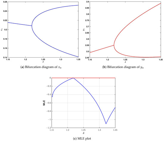
For the above parameters, the critical value for PD bifurcation is ${\delta }_1\approx 1.21804$. The corresponding positive fixed point is $E_1\approx (0.208209,2.54996)$. The eigenvalues of the Jacobian evaluated at $E_1$ are ${\xi }_1=-1$ and ${\xi }_2=-0.349279$, confirming the onset of PD bifurcation as stated in Theorem 3. Furthermore, through detailed computations, we obtain $l_1=-5.91089\ne 0$ and $l_2=14.0297\ne 0$, thereby confirming the conditions stated in Theorem 3. Since $l_2>0$, it follows that a stable period-2 orbit bifurcates from $E_1$.

Figure 1 presents the bifurcation diagrams and the corresponding MLE plot for $\delta \in [1.15,1.35]$. It can be observed that as $\delta$ increases beyond ${\delta }_1$, the system undergoes a cascade of PD bifurcations.

Figure 1. PD bifurcation diagrams and MLE plot of (5) varying $\delta$. The fixed parameter values are $\alpha =2.57,\beta =1.42,\gamma =0.18,\eta =0.25,$ and $\tau =1.85,$ and the initial conditions are $x_0=0.2$ and $y_0=2.5$.

From an ecological standpoint, a higher value of the conversion efficiency $\delta$ implies that predators are more effective in converting consumed prey into their own biomass. For moderate levels of $\delta$, the system typically supports a stable coexistence of both species. In contrast, when $\delta$ attains very large values, it leads to excessive exploitation of the prey population. As a result, the dynamics become oscillatory, with the predator population increasing rapidly and subsequently declining sharply due to prey depletion. This type of recurrent boom-and-bust pattern is commonly observed in ecological settings where predators exhibit an overly strong response to rising prey abundance.

4.1.2. NS Bifurcation

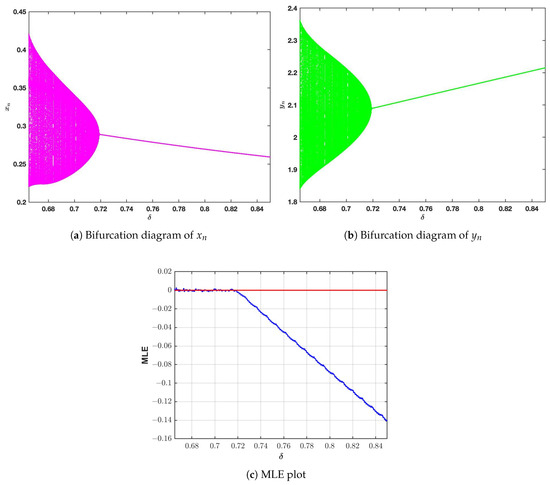
For the same parameter set, the critical value for NS bifurcation is ${\delta }_2\approx 0.718922$. The positive fixed point becomes $E_1\approx (0.288964,2.0888)$, and the eigenvalues ${\xi }_{1,2}=-0.186843\pm 0.98239i$ are complex conjugates with modulus one. This satisfies the condition for NS bifurcation as per Theorem 4.

In addition, detailed computations yield

$$\begin{array}{cc}\hfill {\tau }_{20}& =-0.28714-1.72081i,{\tau }_{11}=-2.03117-1.76539i,\hfill \\ \hfill {\tau }_{02}& =-1.74404-0.04458i,{\tau }_{21}=3.46033+3.00628i.\hfill \end{array}$$

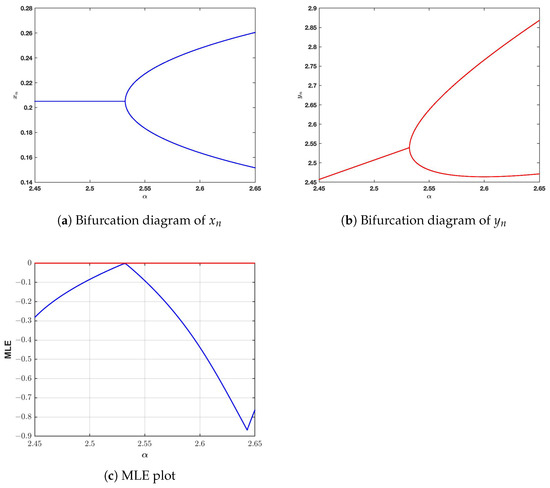
Accordingly, we obtain $L=-3.66543<0$, confirming the validity of Theorem 4. Consequently, the NS bifurcation is supercritical, and an attracting closed invariant curve bifurcates from $E_1$.

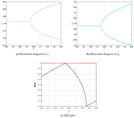
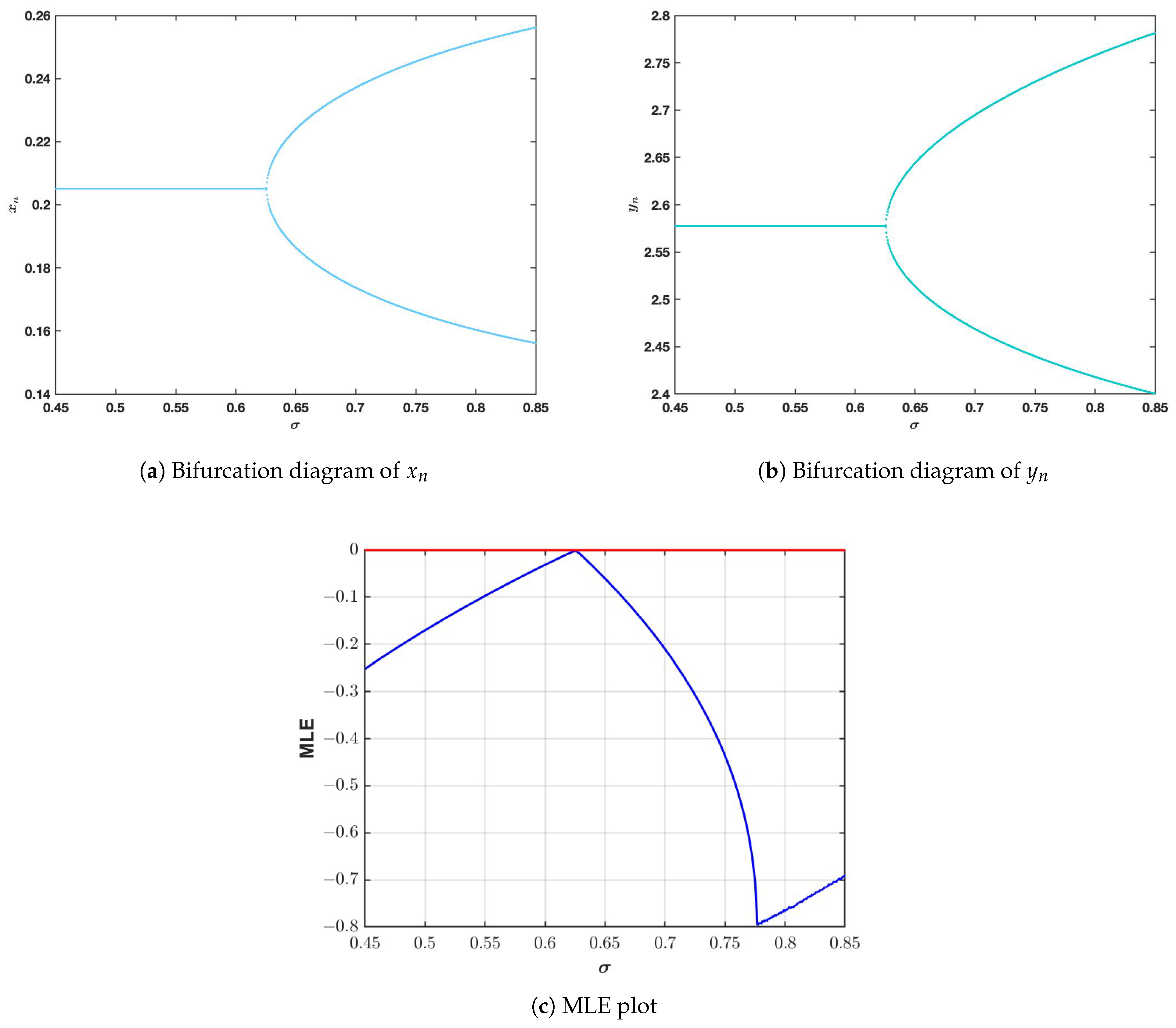
Figure 2 illustrates the bifurcation diagrams and MLE plot for $\delta \in [0.665,0.850]$. As $\delta$ decreases below ${\delta }_2$, the fixed point loses stability and an invariant closed curve emerges, indicating quasiperiodic oscillations.

Figure 2. NS bifurcation diagrams and MLE plot of (5) varying $\delta$. The fixed parameter values are $\alpha =2.57,\beta =1.42,\gamma =0.18,\eta =0.25,$ and $\tau =1.85,$ and the initial conditions are $x_0=0.2$ and $y_0=2.5$.

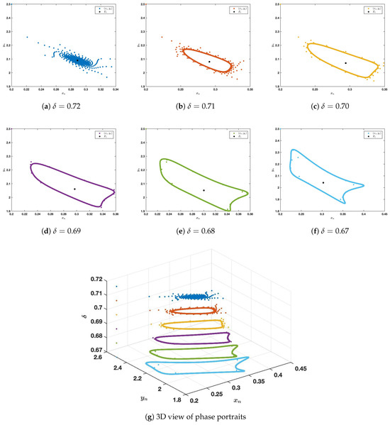
The transition from stability to quasiperiodicity is further depicted in Figure 3a–f, where phase portraits for different values of $\delta$ are shown. Figure 3g provides a three-dimensional view, illustrating how the radius of the invariant curve expands as $\delta$ decreases.

Figure 3. (a–f) Phase portraits of (5) for a few values of $\delta$ by setting $\alpha =2.57,\beta =1.42,\gamma =0.18$, $\eta =0.25,\tau =1.85,x_0=0.2,$ and $y_0=2.5$. (g) The 3D view of phase portraits.

Biologically, the parameter $\delta$ denotes the efficiency of converting consumed prey biomass into predator reproduction. Numerical simulations show that small-to-moderate values of $\delta$ maintain a stable coexistence equilibrium, representing a balanced predator–prey interaction. Once $\delta$ exceeds the PD bifurcation threshold ${\delta }_1$, the predator response becomes overly sensitive to prey availability, destabilizing the equilibrium and inducing oscillatory dynamics. On the other hand, when $\delta$ falls below the NS bifurcation threshold ${\delta }_2$, the equilibrium loses stability through the emergence of quasiperiodic oscillations on invariant closed curves. From a biological standpoint, this corresponds to persistent but bounded population cycles, such as seasonal or multi-year oscillations.

4.2. Bifurcation Analysis with Respect to Parameters $\alpha ,\gamma$

We now analyze how changes in the intrinsic prey growth rate $\alpha$ and predator death rate $\gamma$ affect the system dynamics.

4.2.1. Varying $\alpha$ (Intrinsic Growth Rate of Prey)

From the perspective of ecology, an increase in the growth rate of the prey, denoted by $\alpha$, increases the amount of resources provided to the predator population. However, if the reproduction rate of the prey population is too rapid, it can cause instability between the predator and prey, leading to a recurring pattern where the prey population increases and is then followed by a higher rate of consumption by the predator population, echoing real-life systems where too rapid a growth in resources can cause instability rather than equilibrium stability. Fixing $\delta =1.25$ and other parameters as before, the critical value for PD bifurcation is $\alpha \approx 2.53209$. The corresponding positive fixed point is $E_1\approx (0.205076,2.53947)$ and the eigenvalues of $J\left(E_1\right)$ are ${\xi }_1=-1$ and ${\xi }_2=-0.33527$. Furthermore, after performing detailed computations, we obtain $l_1=-4.75297\ne 0$ and $l_2=13.993016\ne 0$, thereby satisfying the conditions of Theorem 3. Since $l_2>0$, it follows that a stable period-2 orbit bifurcates from $E_1$. Figure 4 shows the bifurcation diagrams and MLE plot for $\alpha \in [2.45,2.65]$. The system exhibits PD bifurcation as $\alpha$ crosses the critical value $2.53209$.

Figure 4. Bifurcation diagrams and MLE plot of (5) varying $\alpha$. The fixed parameter values are $\delta =1.25,\beta =1.42,\gamma =0.18,\eta =0.25,$ and $\tau =1.85,$ and the initial conditions are $x_0=0.2$ and $y_0=2.5$.

Note that the parameter $\alpha$ is the intrinsic growth rate of prey. The above analysis demonstrates that when $\alpha$ is sufficiently small, then prey reproduce at a modest rate, and predators can control the prey density through predation and maintain a coexistence equilibrium that is stable. For large values of $\alpha$, prey reproduce prolifically, providing ample supply of food to predators. This abundance in supply triggers overexploitation cycles of rapid growth of predators followed by depletion of prey and decline of predators, causing PD bifurcation.

4.2.2. Varying $\gamma$ (Predator Death Rate)

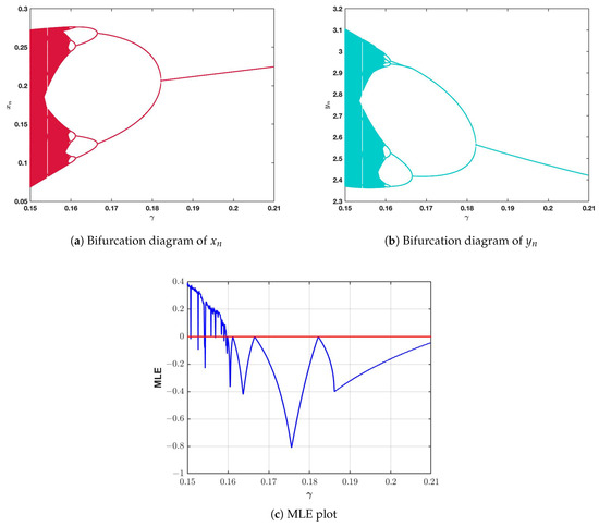
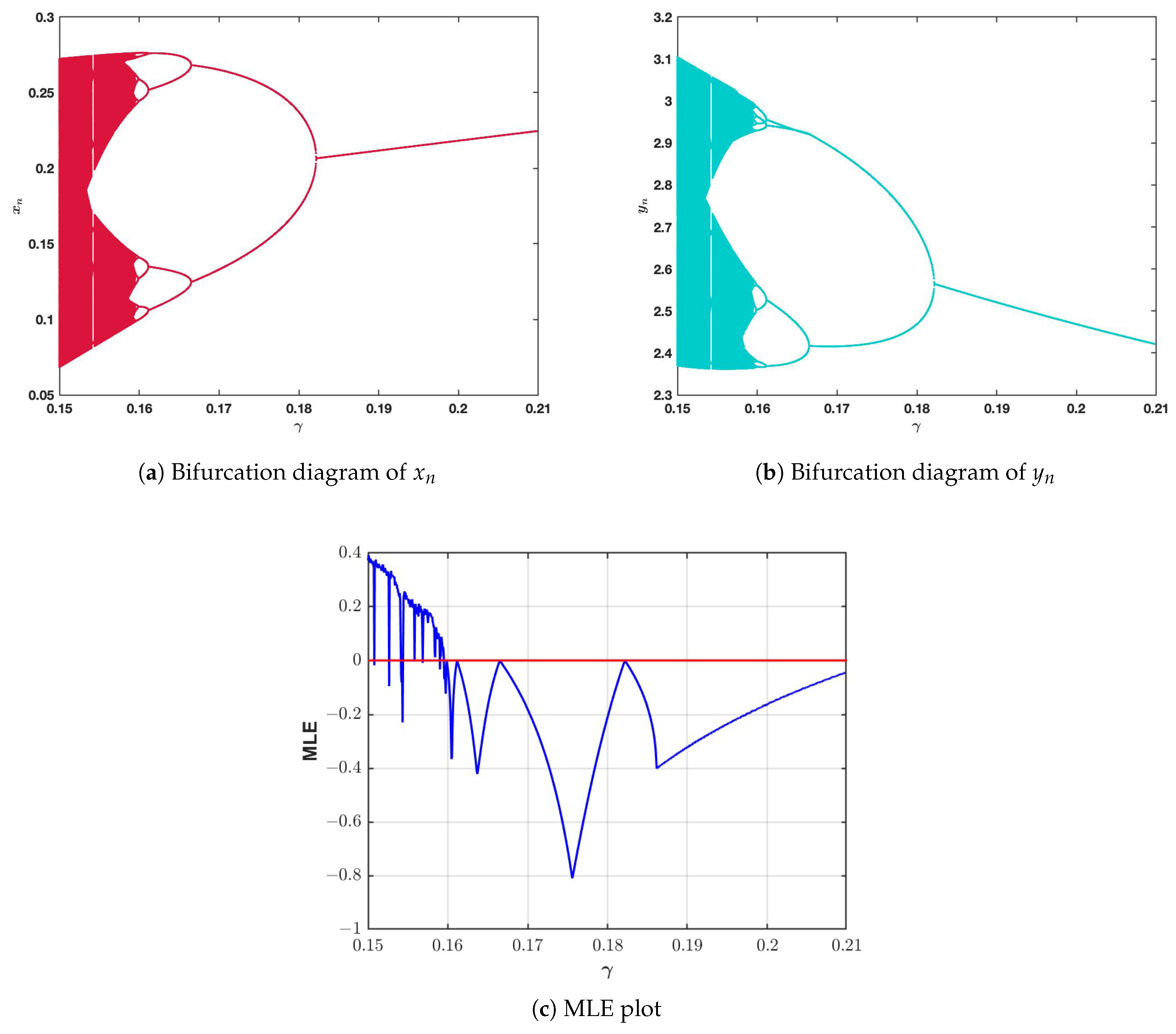
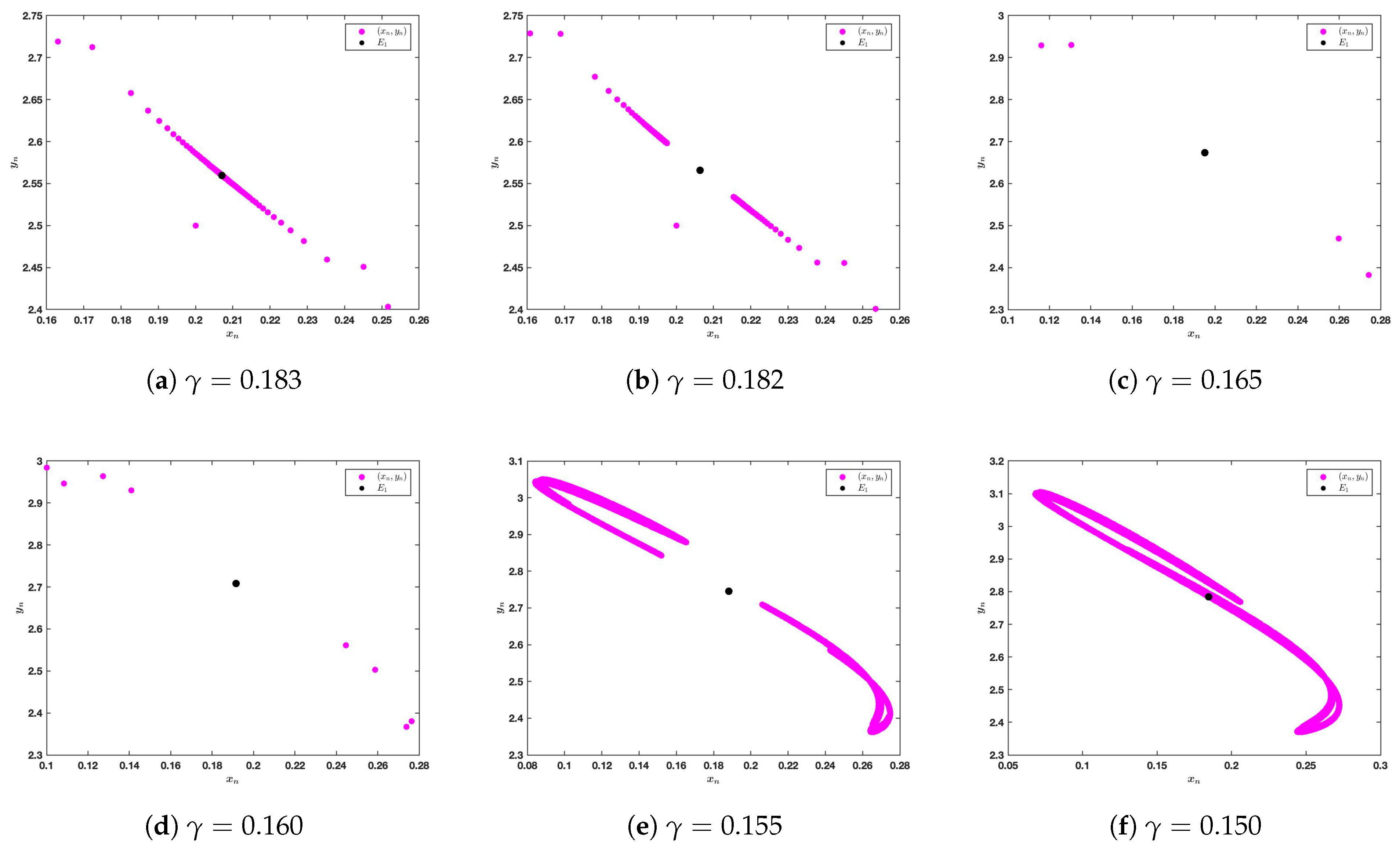
In this context, the predator mortality rate, denoted by $\gamma$, plays an important role as one of the regulating factors for maintaining ecological balance. For example, if the value of $\gamma$ is high, it controls the unceasing growth of the predator population, which in turn reduces undue pressure on the prey population. On the other hand, if the value of $\gamma$ is small, then the predators survive for longer periods, thereby increasing pressure on the prey population, which may cause irregular oscillations, including chaotic behavior, as discussed above, which can be related to ecological models where predators face minimal constraints on their mortality rate. For $\delta =1.25$, the PD bifurcation occurs at $\gamma \approx 0.182161$, with $E_1\approx (0.206512,2.56474)$ and eigenvalues of $J\left(E_1\right)$ are ${\xi }_1=-1$ and ${\xi }_2=-0.368763$. Moreover, through careful evaluation, we obtain $l_1=87.6971\ne 0$ and $l_2=13.8924\ne 0$, confirming that the requirements of Theorem 3 are fulfilled. Since $l_2>0$, it follows that a stable period-2 orbit emerges from $E_1$.

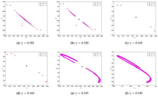
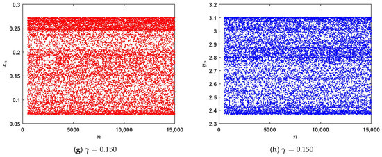
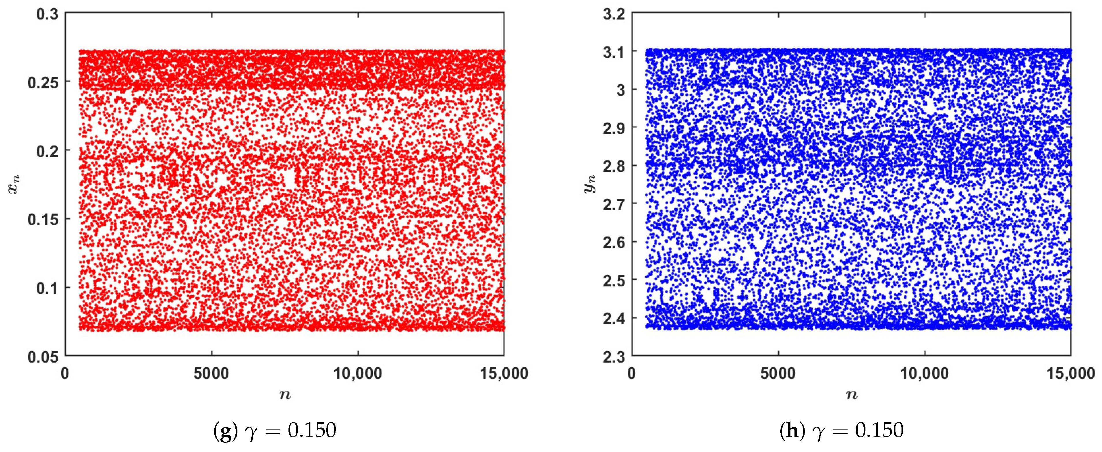
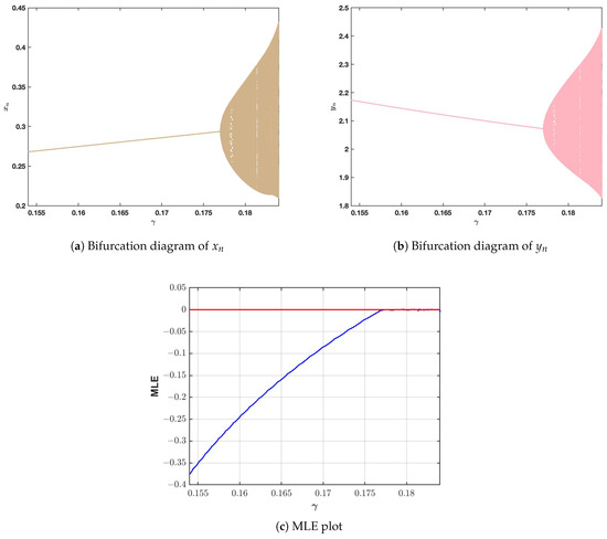
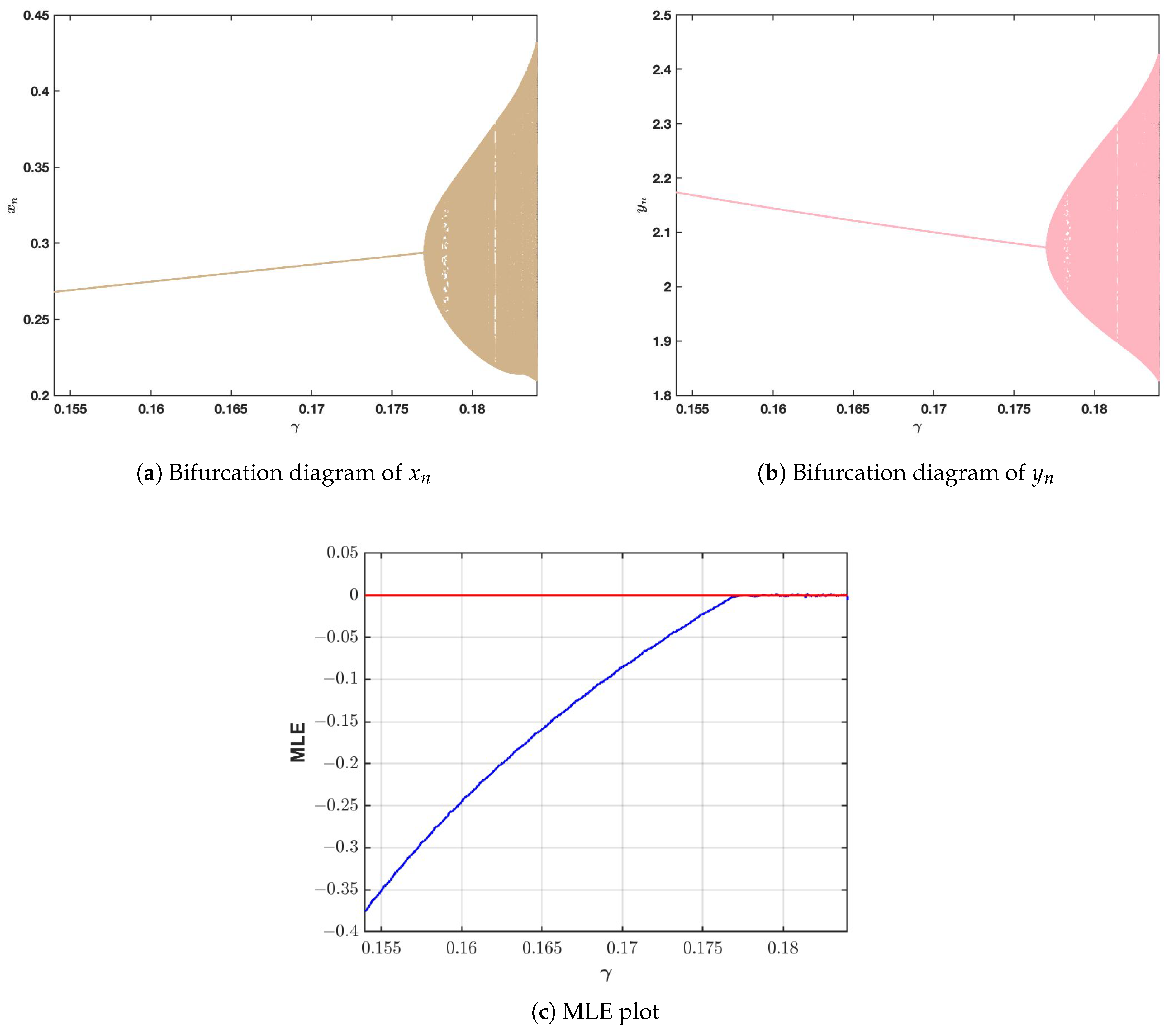
Figure 5 shows bifurcation diagrams and the plot of MLE as $\gamma$ varies from $0.15$ to $0.21$. As $\gamma$ is reduced, the MLE becomes positive for smaller values and indicates that chaotic dynamics will occur for smaller values of $\gamma$, as can be seen in Figure 5c. Figure 6a–f depict a sequence of phase portraits capturing the route from periodic cycles to chaotic attractors. Along with that, time series plots in Figure 6g,h further confirm irregular non-repeating oscillations in both prey and predator populations.

Figure 5. Bifurcation diagrams and MLE plot of (5) varying $\gamma$. The fixed parameter values are $\alpha =2.57,\beta =1.42,\delta =1.25,\eta =0.25,$ and $\tau =1.85,$ and the initial conditions are $x_0=0.2$ and $y_0=2.5$.

Figure 6. (a–f) Phase portraits for some values of $\gamma$ by fixing $\alpha =2.57,\beta =1.42,\delta =1.25,\eta =0.25$, $\tau =1.85,x_0=0.2,$ and $y_0=2.5$. (g) Time series plot for $x_n$; (h) time series plot for $y_n$.

For $\delta =0.69$ (NS case), the bifurcation occurs at $\gamma \approx 0.177011$. The corresponding positive fixed point is $E_1\approx (0.293708,2.07209)$ and the eigenvalues of $J\left(E_1\right)$ are ${\xi }_{1,2}=-0.15754\pm 0.987513i$. Furthermore, detailed calculations yield

$$\begin{array}{cc}\hfill {\tau }_{20}& =-0.33234-1.71678i,{\tau }_{11}=-2.08071-1.74897i,\hfill \\ \hfill {\tau }_{02}& =-1.74836-0.03219i,{\tau }_{21}=3.45324+2.88111i.\hfill \end{array}$$

Accordingly, we obtain $L=-3.81647<0$, which confirms the validity of Theorem 4. Hence, the NS bifurcation is supercritical, and an attracting closed invariant curve originates from $E_1$.

Figure 7 shows the corresponding bifurcation diagrams and MLE plot for $\gamma \in [0.154,0.184]$, where the system transitions from stable focus to quasiperiodic oscillations as $\gamma$ decreases.

Figure 7. Bifurcation diagrams and MLE plot of (5), varying $\gamma$ and fixing $\alpha =2.57,\beta =1.42$, $\delta =0.69,\eta =0.25,\tau =1.85,x_0=0.2,$ and $y_0=2.5$.

The predator mortality rate $\gamma$ plays a stabilizing role in the system dynamics. A sufficiently large $\gamma$ ensures that the growth of the predator is checked in order to maintain a stable coexistence equilibrium. Conversely, the smaller the $\gamma$, the better the survival of the predator, resulting in more predation of the prey. Chaotic behavior has been simulated for the PD bifurcations when the $\gamma$ is decreased. In the regimes of the NS bifurcations, the changes in the $\gamma$ result in quasiperiodic behavior, which can be interpreted as the delayed response of the predator or the complexity of the predator–prey interactions.

4.3. Bifurcation Analysis Varying Fractional-Order $\sigma$

From a biological perspective, the fractional order $\sigma$ signifies the memory effects’ intensity in the system. As the value of $\sigma$ decreases, the memory effects intensify, implying that the past population levels significantly impact the current population levels, thus causing smooth population behavior in the system. This can be described as ecological inertia, where the memory effects act to dampen sudden population level fluctuations. As the value of $\sigma$ increases, the memory effects weaken, causing the system to be dominated by the current population levels. This may lead to destabilization of the equilibrium, causing quasiperiodic and chaotic population oscillations, which may be attributed to ecosystems that face rapidly changing environmental conditions.

In this subsection, the impact of the fractional order $\sigma$ on the dynamics of the system (5) is examined. Even though $\sigma$ appears in the formulation via $\tau ={\displaystyle \frac{h^{\sigma }}{\Gamma (\sigma +1)}}$, it is chosen as the bifurcation parameter in order to explicitly analyze the impact of $\sigma$ on the system’s dynamics. This choice of bifurcation parameter allows us to analyze the role of memory in the transition from the stable stationary state to the oscillatory/chaotic state. Moreover, the analysis is generalized to the non-commensurate case, where different fractional orders of the derivative operators are chosen for the prey and predator species populations, providing a more realistic model of systems with different memory properties. The obtained results indicate that variations in $\sigma$ (as well as ${\sigma }_1$ and ${\sigma }_2$) can trigger NS and PD bifurcations, ultimately leading to chaotic dynamics.

From an ecological perspective, the non-commensurate formulation represents scenarios in which prey and predator populations possess distinct memory characteristics. For example, prey species may respond rapidly to environmental variations, whereas predators may exhibit delayed responses due to biological factors such as gestation periods or learning processes. The findings suggest that these disparities in memory can strongly influence system stability and may give rise to oscillatory or chaotic behavior. This emphasizes the crucial role of heterogeneous memory effects in shaping ecological dynamics.

4.3.1. NS Bifurcation

We consider the parameter set $\alpha =2.57,\beta =1.42,\gamma =0.18,\eta =0.25,\delta =0.69,$ and $h=2.1$. For these values, the NS bifurcation occurs at $\sigma =0.647991$. The associated positive equilibrium point is given by $E_1=(0.297044,2.06083)$. Evaluating the Jacobian matrix at $E_1$ yields a pair of complex conjugate eigenvalues ${\xi }_{1,2}=-0.104613\pm 0.994516i$, whose modulus is unity.

In addition, detailed computations provide

$$\begin{array}{cc}\hfill {\tau }_{20}& =-0.33234-1.71678i,{\tau }_{11}=-2.08071-1.74897i,\hfill \\ \hfill {\tau }_{02}& =-1.74836-0.03219i,{\tau }_{21}=3.45324+2.88111i.\hfill \end{array}$$

Hence, we obtain $L=-3.81647<0$, thereby validating Theorem 4. Consequently, the NS bifurcation is supercritical, and an attracting closed invariant curve bifurcates from $E_1$.

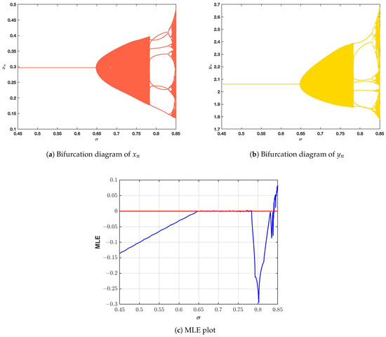
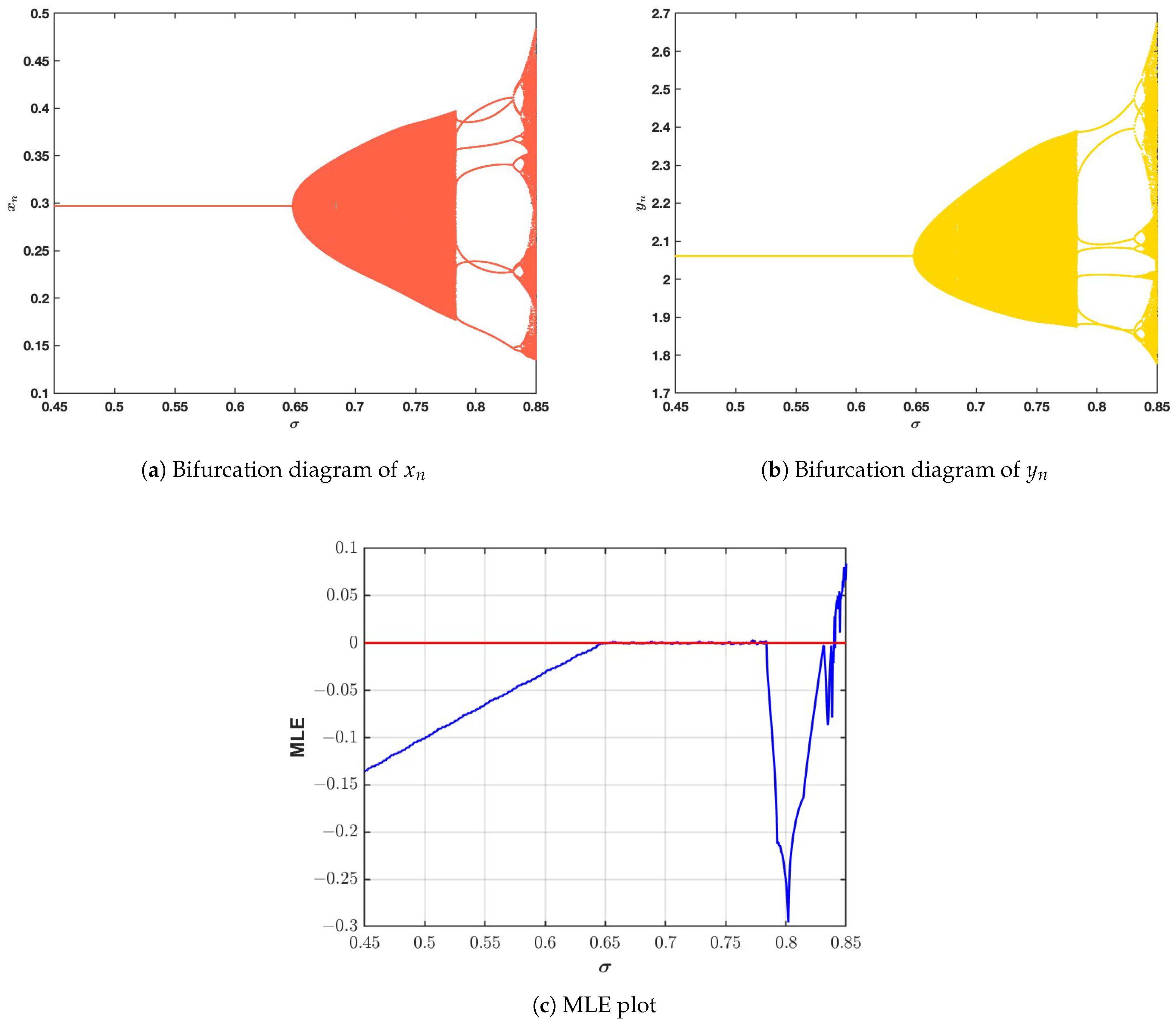
Figure 8 illustrates the bifurcation diagrams and MLE plot for $\sigma \in [0.45,0.85]$. As $\sigma$ increases above $0.647991$, the fixed point loses stability and an invariant closed curve emerges, indicating quasiperiodic oscillations.

Figure 8. Bifurcation diagrams and MLE plot of (5) varying $\sigma$. The fixed parameter values are $\alpha =2.57,\beta =1.42,\gamma =0.18,\eta =0.25,\delta =0.69,$ and $h=2.1,$ and the initial conditions are $x_0=0.3$ and $y_0=2.1$.

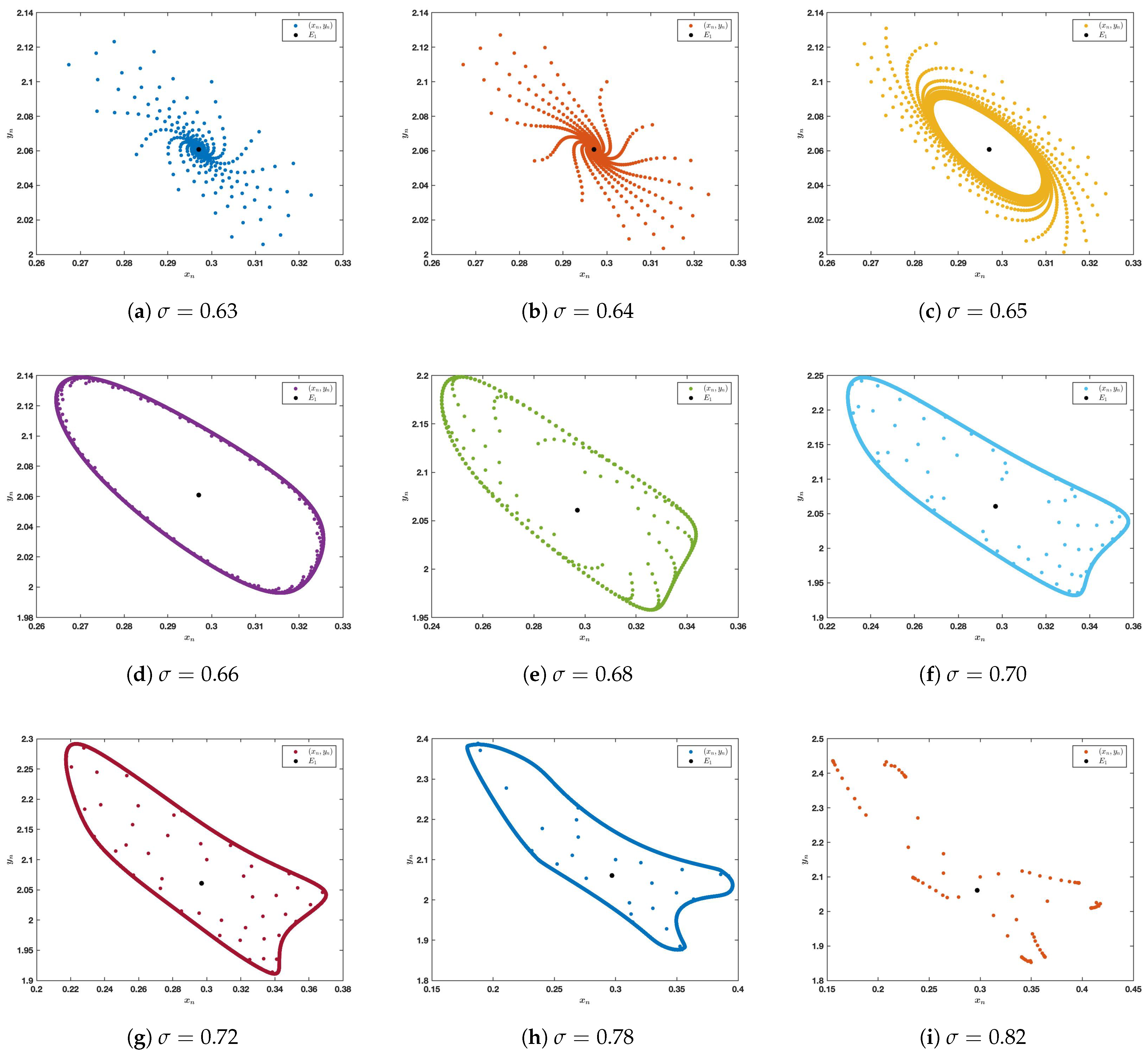
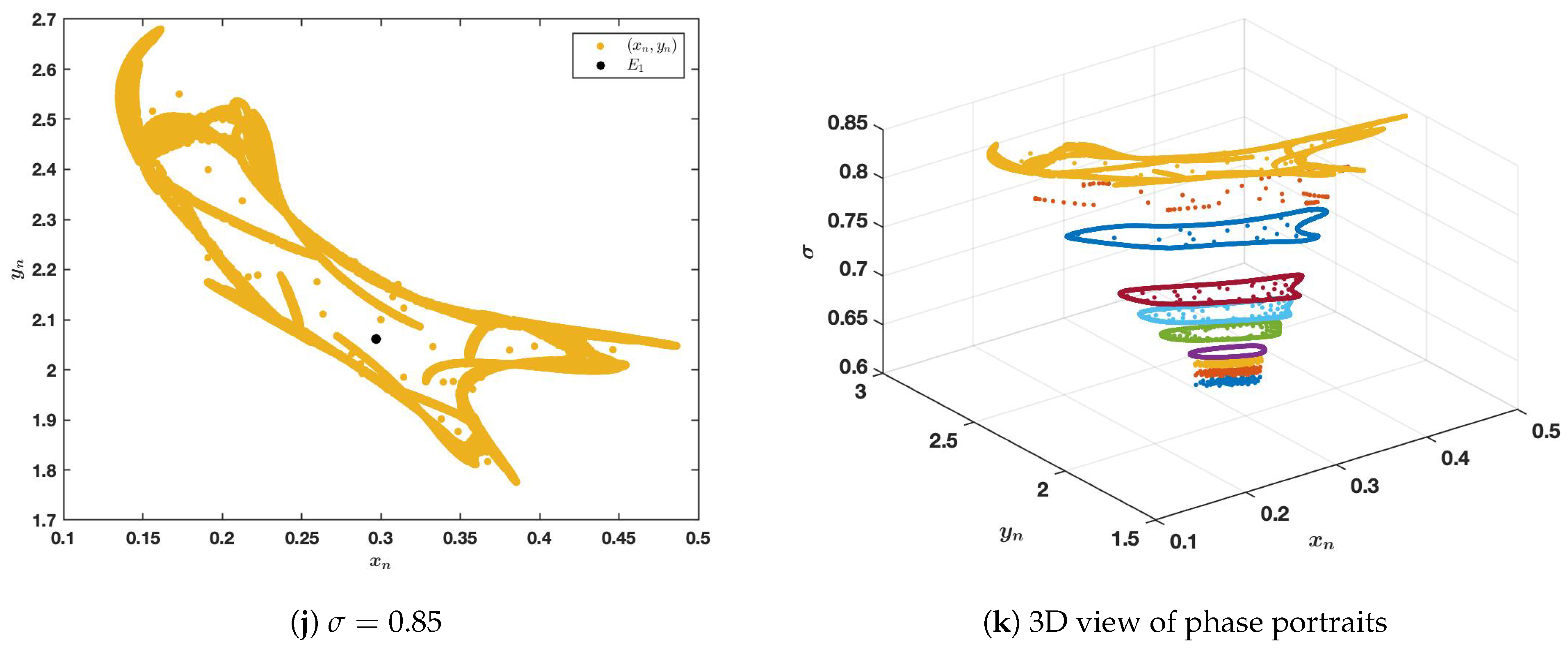
As seen in Figure 8, when $\sigma <0.647991$, all trajectories converge to the equilibrium point $E_1$. Additionally, in Figure 8a,b, where bifurcation diagrams for different variables are shown, a single branch is seen for all values of $\sigma$. However, as the value of $\sigma$ is increased to approach 0.647991, in Figure 8c, where MLE is shown, it is seen that MLE tends to zero. This is an indication that stability is lost for the equilibrium point. When $\sigma >0.647991$, bifurcation diagrams for different variables are seen to broaden in Figure 8a,b, indicating that oscillations have begun in the system. This is an indication of NS bifurcation, where a stable fixed point loses stability and a closed invariant curve is created, resulting in quasiperiodic oscillations. Additionally, in Figure 8c, when values of $\sigma$ are increased, MLE is seen to become positive. This is an indication that the system is transitioning from quasiperiodic behavior to chaotic behavior, where random fluctuations in both prey and predator populations can be seen.

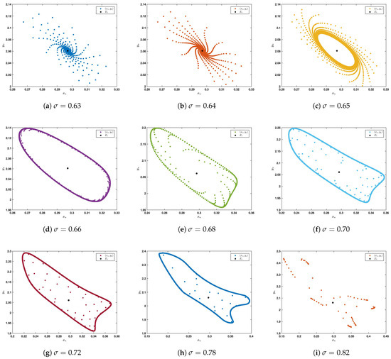
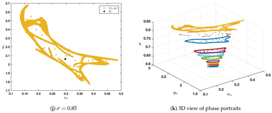
The phase portraits for increasing values of $\sigma$ are given in Figure 9a–j. These phase portraits confirm the transition from the stable state to quasiperiodic and chaotic states. In the phase portraits for $\sigma =0.63$ and $\sigma =0.64$ (Figure 9a,b), it can be seen that the trajectories converge to the fixed point $E_1$, confirming the stability of this fixed point. In the phase portrait for $\sigma =0.65$ (Figure 9c), an invariant closed curve around the fixed point $E_1$ can be seen, confirming the loss of stability of the fixed point $E_1$ for this value of $\sigma$ corresponding to quasiperiodic motion. In the phase portraits for increasing values of $\sigma$ (Figure 9d–i), the size of the invariant curve increases with increasing values of $\sigma$, confirming the increase in the level of quasiperiodic motion. Finally, the strange chaotic attractor for $\sigma =0.85$ is given in Figure 9j, confirming the positive maximum Lyapunov exponent as given in Figure 8c. A three-dimensional visualization of these phase portraits is provided in Figure 9k, clearly showing that the size of the invariant curve grows with increasing $\sigma$.

Figure 9. (a–j) Phase portraits for some values of $\sigma$ by fixing $\alpha =2.57,\beta =1.42,\gamma =0.18,\eta =0.25$, $\delta =0.69,h=2.1,x_0=0.3,$ and $y_0=2.1$. (k) A 3D view of phase portraits.

The parameter $\sigma$ measures the intensity of memory effects in the predator–prey system. The lower the value of $\sigma$, the higher the memory intensity, meaning that the current growth and predation processes are significantly affected by the past population levels. This causes the system to be more stable, allowing it to converge to the equilibrium $E_1$. As the value of $\sigma$ increases, the memory intensity decreases, meaning that the system is more sensitive to the current state. This causes the delayed feedback loops to destabilize the equilibrium by an NS bifurcation, resulting in quasiperiodic oscillations along the invariant closed curves. As the value of $\sigma$ further increases, chaotic motion results from the quasiperiodic oscillations. The value of $\sigma$ thus acts as a bifurcation parameter in the predator–prey system, causing the system to transition from a stable state of coexistence to quasiperiodic and chaotic motion.

4.3.2. PD Bifurcation

We assume $\alpha =2.57,\beta =1.42,\gamma =0.18,\eta =0.25,\delta =1.25,$ and $h=2.1$. For this set of parameter values, the PD bifurcation takes place for $\sigma =0.625725$. The positive equilibrium point for this set of parameter values is given by the point $E_1=(0.205076,2.57749)$. The eigenvalues of the Jacobian matrix for the equilibrium point $E_1=(0.205076,2.57749)$ are ${\xi }_1=-1$ and ${\xi }_2=-0.246395$, which confirm the occurrence of the PD bifurcation, as discussed in Theorem 3. The bifurcation diagrams along with the MLE plot for $\sigma \in [0.45,0.85]$ are depicted in Figure 10. It is obvious from the figure that for $\sigma >0.625725$, the equilibrium point loses stability via the PD bifurcation. For $\sigma <0.625725$, the bifurcation diagram has a single branch, implying the stability of the equilibrium point. This implies the convergence of the trajectories to the equilibrium point. Therefore, as the parameter $\sigma$ approaches $0.625725$, the eigenvalue ${\xi }_1$ crosses $-1$, resulting in the creation of the stable periodic orbit of period 2. The bifurcation diagrams along with the MLE plot for the given range of $\sigma \in [0.45,0.85]$ are given in Figure 10c.

Figure 10. Bifurcation diagrams and MLE plot of (5) varying $\sigma$. The fixed parameter values are $\alpha =2.57,\beta =1.42,\gamma =0.18,\eta =0.25,\delta =1.25,$ and $h=2.1,$ and the initial conditions are $x_0=0.2$ and $y_0=2.5$.

4.3.3. Bifurcation Analysis of the Non-Commensurate Fractional-Order Model

We consider the following non-commensurate fractional model:

$$\left\{\begin{array}{c}{x}_{n+1}=x_n+{\displaystyle \frac{h^{{\sigma }_1}}{\Gamma ({\sigma }_1+1)}}\left(\alpha x_n-{\displaystyle \frac{\beta x_n^2{y}_n}{x_n^2+\eta }}\right),\hfill \\ y_{n+1}=y_n+{\displaystyle \frac{h^{{\sigma }_2}}{\Gamma ({\sigma }_2+1)}}\left(-\gamma y_n+{\displaystyle \frac{\delta x_n^2{y}_n}{x_n^2+\eta }}\right),\hfill \end{array}\right.$$

(24)

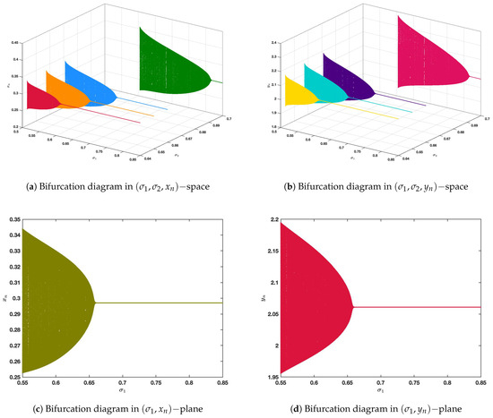
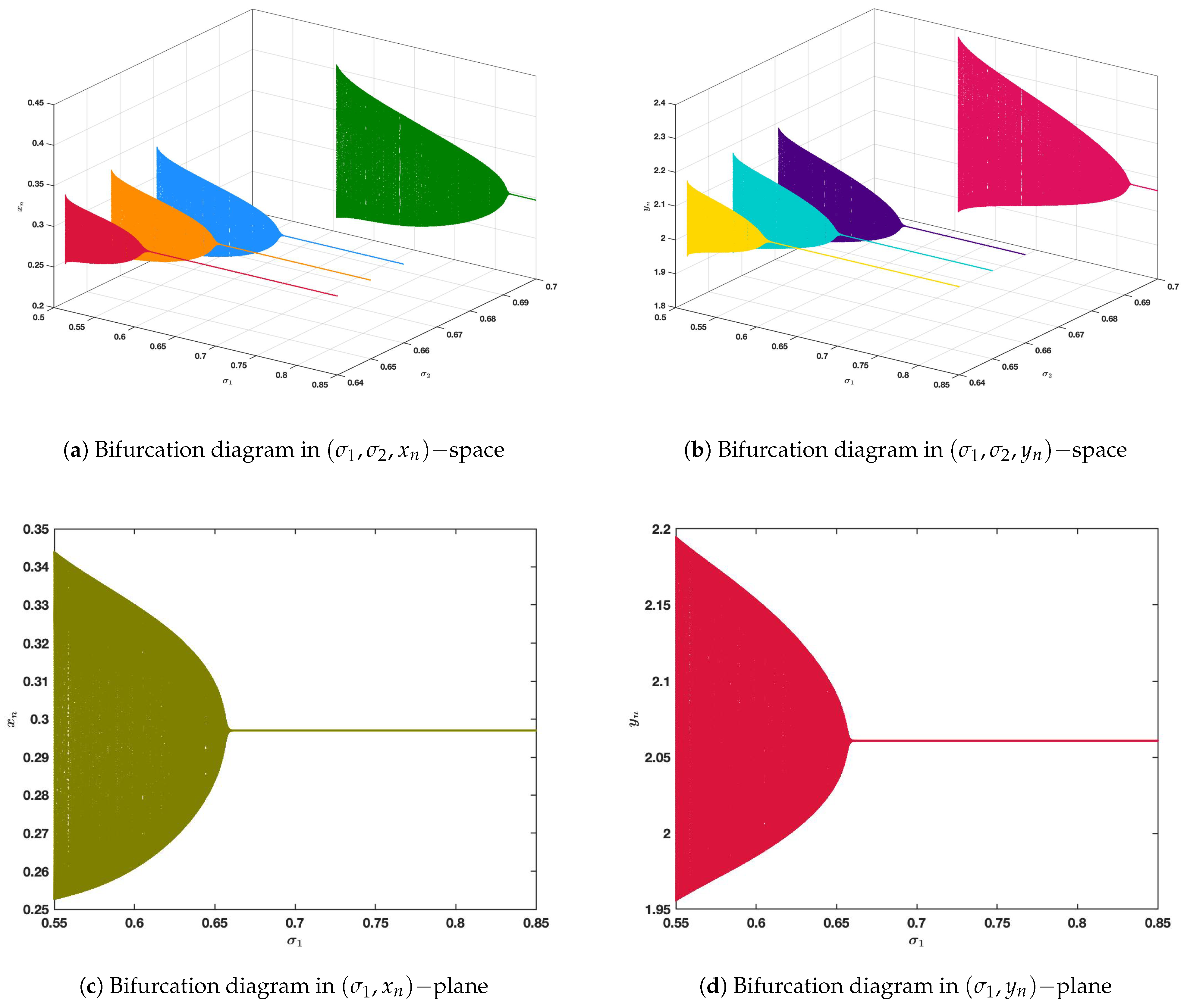
We consider the parameter set $\alpha =2.57,\beta =1.42,\gamma =0.18,\eta =0.25,\delta =0.69,$ and $h=2.1$. The bifurcation diagrams shown in Figure 11a,b are obtained by varying ${\sigma }_1\in [0.45,0.85]$ and ${\sigma }_2\in [0.64,0.70]$, with initial conditions $x_0=0.3$ and $y_0=2.1$. Furthermore, Figure 11c,d display the bifurcation structure when ${\sigma }_2$ is fixed at $0.65$, while ${\sigma }_1$ is varied over the interval $[0.55,0.85]$, using the same set of initial values.

Figure 11. Bifurcation diagrams of (24) with respect to ${\sigma }_1$ and ${\sigma }_2$, showing the influence of non-commensurate fractional orders on system dynamics. The fixed parameter values are $\alpha =2.57,\beta =1.42,\gamma =0.18,\eta =0.25,\delta =0.69,$ and $h=2.1,$ and the initial conditions are $x_0=0.3$ and $y_0=2.1$.

As can be seen in Figure 11, different values of non-commensurate fractional orders can greatly change the bifurcation diagram of the system. If both ${\sigma }_1$ and ${\sigma }_2$ are varied, different dynamic regimes are observed, depending on how the memory of the prey species (${\sigma }_1$) and the memory of the predator species (${\sigma }_2$) are related. Moreover, if ${\sigma }_2$ is fixed and ${\sigma }_1$ is varied, it can be seen that the bifurcation diagram changes significantly, as shown in Figure 11c,d. This again confirms that changing the memory of the prey species alone can drive a transition from a stable steady state to oscillatory and more complex.

From an ecological viewpoint, the non-commensurate form allows for the presence of different memory strengths for the prey and predator populations, giving rise to a more realistic model since different species can have different responses to past environmental conditions, success of predation, and availability of resources. The numerical results show that even small differences in ${\sigma }_1$ and ${\sigma }_2$ lead to an extension of the oscillations and the stability domain of coexistence. Thus, the asymmetric memory effect can lead to increased instability and more complex behavior in comparison to the commensurate model. The results emphasize the importance of $\sigma$, ${\sigma }_1$, and ${\sigma }_2$ as key bifurcation parameters.

4.4. Two-Parameter Analysis

To further explore the global dynamics, we perform two-parameter bifurcation analysis.

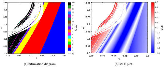
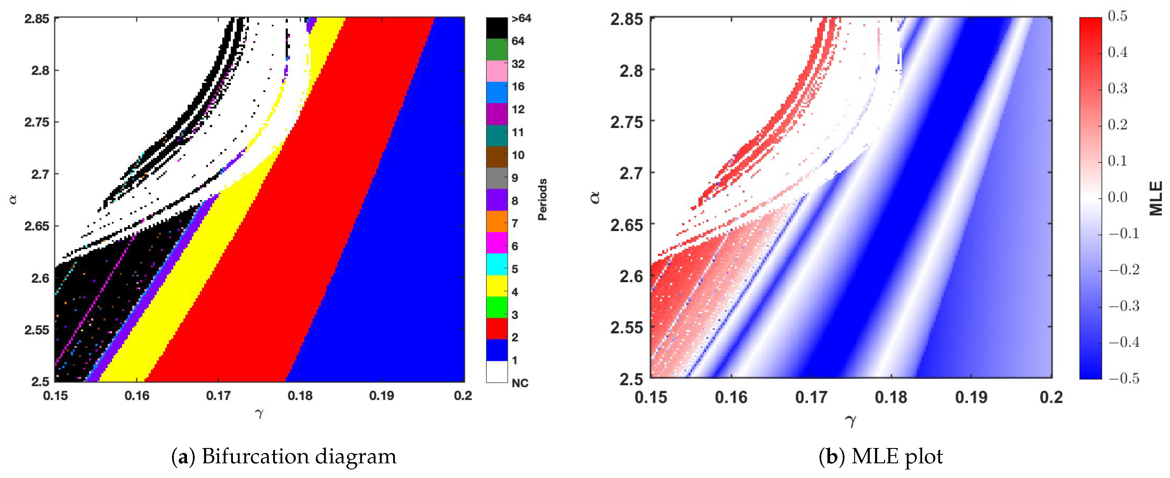
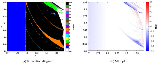
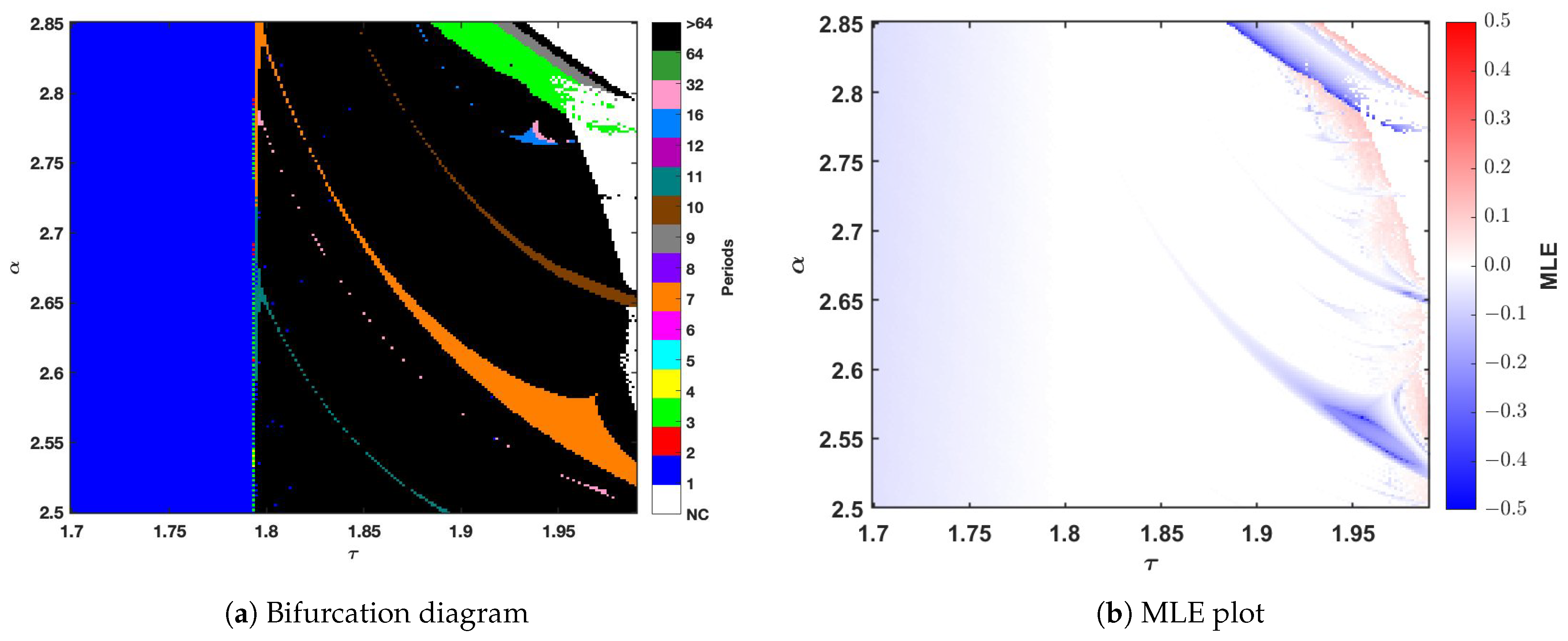
Fixing $\beta =1.42,\delta =1.25,\eta =0.25,\tau =1.85,x_0=0.2,$ and $y_0=2.5$, we vary $\alpha \in [2.50,2.85]$ and $\gamma \in [0.15,0.20]$. Figure 12a presents a two-dimensional bifurcation diagram in the $(\gamma ,\alpha )$-plane where different colors are showing different periodic regions. Figure 12b presents the corresponding two-dimensional MLE plot in the $(\gamma ,\alpha )$-plane.

Figure 12. Two-dimensional bifurcation diagram and MLE plot of (5) varying $\alpha \in [2.50,2.85]$ and $\gamma \in [0.15,0.20]$. The fixed parameter values are $\beta =1.42,\delta =1.25,\eta =0.25,$ and $\tau =1.85,$ and initial values are $x_0=0.2$ and $y_0=2.5$.

Fixing $\beta =1.42,\gamma =0.18,\eta =0.25,\delta =0.69,x_0=0.2,$ and $y_0=2.5$, we vary $\alpha \in [2.50,2.85]$ and $\tau \in [1.70,1.99]$. Figure 13a presents a two-dimensional bifurcation diagram in the $(\tau ,\alpha )$-plane where different colors are showing different periodic regions. Figure 13b presents the corresponding two-dimensional MLE plot in the $(\tau ,\alpha )$-plane.

Figure 13. Two-dimensional bifurcation diagram and MLE plot of (5) varying $\alpha \in [2.50,2.85]$ and $\tau \in [1.70,1.99]$. The fixed parameter values are $\beta =1.42,\gamma =0.18,\eta =0.25,$ and $\delta =0.69,$ and the initial values are $x_0=0.2$ and $y_0=2.5$.

Two-parameter bifurcation analysis helps provide a global insight into the interaction of various ecological factors that influence the dynamics of the system. The two-parameter bifurcation diagram shows that the system includes regions with various dynamic behaviors, namely stable equilibrium points, periodic solutions, quasiperiodic oscillations, and chaos, emphasizing that the system is quite sensitive to parameter values. Ecological interpretation shows that ecological systems are characterized by sudden transitions from stability to chaos and vice versa with even minute changes in environmental factors. This evidence is supported by similar patterns in bifurcations and MLE that emphasize regions with chaos as regions with utterly unpredictable patterns and regions with quasiperiodic oscillations as regions with complex patterns. This two-parameter bifurcation analysis provides evidence that discrete fractional models have the capability to capture the complex but unpredictable nature of actual ecosystems in a much better way compared to traditional continuous models.

5. Conclusions

In this work, we examined the dynamical behavior of a discretized fractional-order predator–prey model incorporating a Holling type III functional response. The discrete system was derived from a biologically relevant fractional-order continuous model using the piecewise constant argument method, which allows memory effects to be embedded into a discrete-time framework. Such a formulation offers a realistic representation of predator–prey interactions in ecosystems where historical population levels affect current dynamics and population changes occur at discrete time intervals.

This analysis begins with the study of the existence and stability of equilibrium points in the discrete-time model (5). The stability and instability conditions in terms of eigenvalue restrictions were found by evaluating the Jacobian matrix. The stability and instability analysis focused on the positive fixed point, where rigorous analytical conditions for the occurrence of PD and NS bifurcations are established.

Numerical simulations, such as bifurcation diagrams, phase portraits, time series, as well as MLE calculations, confirmed the findings of the analytical work and showed the occurrence of bifurcations from stable fixed points to periodic, quasiperiodic, and chaotic motion. Furthermore, the two-parameter bifurcation diagram offered a global description of the system’s behavior by locating the regions of the parameter plane where the system exhibits stability, periodic motion, quasiperiodicity, and chaotic motion. In addition, the non-commensurate fractional-order case was also examined, where it was found that different memory indices for the prey and predator populations can enhance the complexity of the system’s behavior and greatly affect the stability and bifurcation of the system.

From the ecological perspective, the quasiperiodic and chaotic behavior of the system may suggest irregular and unpredictable population oscillations, which may possibly lead to population crashes or outbreaks. The existence of chaos may also suggest sensitivity to initial conditions, which makes it difficult for such systems to be managed sustainably.

The results also highlight the significant impact of memory effects on the system’s dynamics. Specifically, it can be seen that higher memory, i.e., smaller values of the fractional order $\sigma$, has a dampening effect on the system’s fluctuations, stabilizing the system’s behavior, whereas lower memory, i.e., higher values of the fractional order $\sigma$, has a destabilizing impact, leading to complex oscillations and chaotic behavior in the system’s evolution. Additionally, the non-commensurate formulation indicates that disparities in memory between species can modify interaction mechanisms and increase the potential for complex behavior. Although the Holling type III functional response contributes to stabilization at low prey densities, its combined effect with memory and discrete-time dynamics can generate a wide range of intricate dynamical patterns.

This study demonstrates that the combined effects of nonlinear functional response, fractional-order memory (in both commensurate and non-commensurate forms), and discretization can produce a wide spectrum of dynamical behaviors in predator–prey systems. The developed framework contributes to a deeper understanding of discrete fractional-order ecological models and offers a solid foundation for future research that incorporates additional biological factors and effective management strategies.

References

- Lotka, A.J. Elements of physical biology. Nature 1925, 116, 461. [Google Scholar] [CrossRef] [Scilit]
- Volterra, V. Fluctuations in the abundance of a species considered mathematically. Nature 1926, 118, 558–560. [Google Scholar] [CrossRef] [Scilit]
- Zhao, L.; Shen, J. Relaxation oscillations in a slow-fast predator-prey model with weak Allee effect and Holling-IV functional response. Commun. Nonlinear Sci. Numer. Simul. 2022, 112, 106517. [Google Scholar] [CrossRef] [Scilit]
- Sarkar, K.; Khajanchi, S.; Mali, P.C.; Nieto, J.J. Rich dynamics of a predator-prey system with different kinds of functional responses. Complexity 2020, 2020, 4285294. [Google Scholar] [CrossRef] [Scilit]
- Singh, M.K.; Sharma, A.; Sanchez-Ruiz, L.M. Impact of the Allee Effect on the Dynamics of a Predator-Prey Model Exhibiting Group Defense. Mathematics 2025, 13, 633. [Google Scholar] [CrossRef] [Scilit]
- He, T.; Zhang, Y. Stability and bifurcation analysis of a predator-prey model with Allee effect and predator harvesting. Int. J. Bifurc. Chaos 2025, 35, 2550007. [Google Scholar] [CrossRef] [Scilit]
- Kumar, S.; Kharbanda, H. Chaotic behavior of predator-prey model with group defense and non-linear harvesting in prey. Chaos Solitons Fractals 2019, 119, 19–28. [Google Scholar] [CrossRef] [Scilit]
- Suleman, A.; Khan, A.Q.; Ahmed, R. Bifurcation analysis of a discrete Leslie-Gower predator-prey model with slow-fast effect on predator. Math. Methods Appl. Sci. 2024, 47, 8561–8580. [Google Scholar] [CrossRef] [Scilit]
- Alsulami, I.M.; Ahmed, R.; Ashraf, F. Exploring complex dynamics in a Ricker type predator–prey model with prey refuge. Chaos Interdiscip. J. Nonlinear Sci. 2025, 35, 023107. [Google Scholar] [CrossRef] [Scilit] [PubMed]
- Wang, X.; Zanette, L.; Zou, X. Modelling the fear effect in predator-prey interactions. J. Math. Biol. 2016, 73, 1179–1204. [Google Scholar] [CrossRef] [Scilit] [PubMed]
- Li, H.L.; Zhang, L.; Hu, C.; Jiang, Y.L.; Teng, Z. Dynamical analysis of a fractional-order predator-prey model incorporating a prey refuge. J. Appl. Math. Comput. 2016, 54, 435–449. [Google Scholar] [CrossRef] [Scilit]
- Suryanto, A.; Darti, I.; Panigoro, H.S.; Kilicman, A. A fractional-order predator-prey model with ratio-dependent functional response and linear harvesting. Mathematics 2019, 7, 1100. [Google Scholar] [CrossRef] [Scilit]
- Djilali, S.; Ghanbari, B. The influence of an infectious disease on a prey-predator model equipped with a fractional-order derivative. Adv. Differ. Equ. 2021, 2021, 20. [Google Scholar] [CrossRef] [Scilit]
- Hariprasad, S.; Kumar, N.P.; Reddy, K.S.; Acharyulu, K.V.; Srinivas, M.A.; Nisar, K.S. Fractional order Eco-Epidemiological model for the dynamics of a prey-predator system. Model. Earth Syst. Environ. 2025, 11, 186. [Google Scholar] [CrossRef] [Scilit]
- Wei, Z.; Wu, F.; Xue, G.; Lin, F.; Liu, H. Stability analysis and bifurcation control of a fractional order predator prey system. Fractal Fract. 2025, 9, 681. [Google Scholar] [CrossRef] [Scilit]
- Holling, C.S. Some characteristics of simple types of predation and parasitism. Can. Entomol. 1959, 91, 385–398. [Google Scholar] [CrossRef] [Scilit]
- Beddington, J.R. Mutual interference between parasites or predators and its effect on searching efficiency. J. Anim. Ecol. 1975, 44, 331–340. [Google Scholar] [CrossRef] [Scilit] [PubMed]
- DeAngelis, D.L.; Goldstein, R.A.; O’Neill, R.V. A model for tropic interaction. Ecology 1975, 56, 881–892. [Google Scholar] [CrossRef] [Scilit]
- Crowley, P.H.; Martin, E.K. Functional responses and interference within and between year classes of a dragonfly population. J. N. Am. Benthol. Soc. 1989, 8, 211–221. [Google Scholar] [CrossRef] [Scilit]
- Kim, H.K.; Baek, H. The dynamical complexity of a predator-prey system with Hassell-Varley functional response and impulsive effect. Math. Comput. Simul. 2013, 94, 1–14. [Google Scholar] [CrossRef] [Scilit]
- Chen, X.; Zhang, X. Dynamics of the predator-prey model with the Sigmoid functional response. Stud. Appl. Math. 2021, 147, 300–318. [Google Scholar] [CrossRef] [Scilit]
- Arancibia-Ibarra, C.; Aguirre, P.; Flores, J.; van Heijster, P. Bifurcation analysis of a predator-prey model with predator intraspecific interactions and ratio-dependent functional response. Appl. Math. Comput. 2021, 402, 126152. [Google Scholar] [CrossRef] [Scilit]
- Braza, P.A. Predator-prey dynamics with square root functional responses. Nonlinear Anal. Real World Appl. 2012, 13, 1837–1843. [Google Scholar] [CrossRef] [Scilit]
- Kaur, M.; Rani, R.; Bhatia, R.; Verma, G.N.; Ahirwar, S. Dynamical study of quadrating harvesting of a predator-prey model with Monod-Haldane functional response. J. Appl. Math. Comput. 2021, 66, 397–422. [Google Scholar] [CrossRef] [Scilit]
- Yadav, M.; Malik, P.; Uddin, M.J.; Shah, N.A. Modeling and managing chaos: A fear-affected discretized prey-predator system with Allee effect. Eur. Phys. J. Plus 2025, 140, 396. [Google Scholar] [CrossRef] [Scilit]
- Baydemir, P.; Merdan, H.; Karaoglu, E.; Sucu, G. Complex dynamics of a discrete-time prey-predator system with Leslie type: Stability, bifurcation analyses and chaos. Int. J. Bifurc. Chaos 2020, 30, 2050149. [Google Scholar] [CrossRef] [Scilit]
- Sharma, V.S.; Singh, A.; Elsonbaty, A.; Elsadany, A.A. Codimension-one and -two bifurcation analysis of a discrete-time prey-predator model. Int. J. Dyn. Control 2023, 11, 2691–2705. [Google Scholar] [CrossRef] [Scilit]
- Wang, C.; Sun, B.; Zhao, Q. Dynamics of a discrete Rosenzweig-Macarthur predator-prey model with piecewise-constant arguments. Int. J. Biomath. 2024, 2024, 2450121. [Google Scholar] [CrossRef] [Scilit]
- Wang, B.; Li, X. Modeling and dynamical analysis of a fractional-order predator-prey system with anti-predator behavior and a Holling type IV functional response. Fractal Fract. 2023, 7, 722. [Google Scholar] [CrossRef] [Scilit]
- Shi, Y.; Wang, Z. Bifurcation analysis and chaos control of a discrete fractional-order Leslie-Gower model with fear factor. AIMS Math. 2024, 9, 30298–30319. [Google Scholar] [CrossRef] [Scilit]
- Kome, S. Complex dynamics of a discrete fractional-order Leslie-type predator-prey model with constant immigration effect. J. Appl. Math. Comput. 2025, 71, 7863–7904. [Google Scholar] [CrossRef] [Scilit]
- Elsadany, A.A.; Matouk, A.E. Dynamical behaviors of fractional-order Lotka-Volterra predator-prey model and its discretization. J. Appl. Math. Comput. 2015, 49, 269–283. [Google Scholar] [CrossRef] [Scilit]
- Singh, A.; Elsadany, A.A.; Elsonbaty, A. Complex dynamics of a discrete fractional-order Leslie-Gower predator-prey model. Math. Methods Appl. Sci. 2019, 42, 3992–4007. [Google Scholar] [CrossRef] [Scilit]
- Mondal, S.; Biswas, M.; Bairagi, N. Local and global dynamics of a fractional-order predator-prey system with habitat complexity and the corresponding discretized fractional-order system. J. Appl. Math. Comput. 2020, 63, 311–340. [Google Scholar] [CrossRef] [Scilit]
- Panigoro, H.S.; Rayungsari, M.; Suryanto, A. Bifurcation and chaos in a discrete-time fractional-order logistic model with Allee effect and proportional harvesting. Int. J. Dyn. Control 2023, 11, 1544–1558. [Google Scholar] [CrossRef] [Scilit]
- Uddin, M.J.; Podder, C.N. Fractional order prey-predator model incorporating immigration on prey: Complexity analysis and its control. Int. J. Biomath. 2024, 17, 2350051. [Google Scholar] [CrossRef] [Scilit]
- Kilbas, A.A.; Srivastava, H.M.; Trujillo, J. Theory and Applications of Fractional Differential Equations; North-Holland Mathematics Studies; Elsevier: Amsterdam, The Netherlands, 2006; Volume 204. [Google Scholar] [CrossRef] [Scilit]
- Catalan-Angeles, G.; Arciga-Alejandre, M.P.; Sanchez-Ortiz, J. Fractional Lotka-Volterra model with Holling type III functional response. Math. Methods Appl. Sci. 2023, 46, 17128–17136. [Google Scholar] [CrossRef] [Scilit]
- Ahmed, R.; Yazdani, M.S. Complex dynamics of a discrete-time model with prey refuge and Holling type-II functional response. J. Math. Comput. Sci. 2022, 12, 113. [Google Scholar] [CrossRef] [Scilit]
- Almatrafi, M.B.; Berkal, M.; Ahmed, R. Dynamical transitions and chaos control in a discrete predator–prey model with Gompertz growth and Holling type III response. Chaos Solitons Fractals 2025, 200, 117071. [Google Scholar] [CrossRef] [Scilit]
- Guckenheimer, J.; Holmes, P. Nonlinear Oscillations, Dynamical Systems, and Bifurcations of Vector Fields; Springer: New York, NY, USA, 1983; Volume 42. [Google Scholar] [CrossRef] [Scilit]
- Wiggins, S.; Golubitsky, M. Introduction to Applied Nonlinear Dynamical Systems and Chaos; Springer: New York, NY, USA, 2003; Volume 2. [Google Scholar] [CrossRef] [Scilit]
- Jing, Z.; Yang, J. Bifurcation and chaos in discrete-time predator-prey system. Chaos Solitons Fractals 2006, 27, 259–277. [Google Scholar] [CrossRef] [Scilit]
- Zhang, G.; Shen, Y.; Chen, B. Bifurcation analysis in a discrete differential-algebraic predator-prey system. Appl. Math. Model. 2014, 38, 4835–4848. [Google Scholar] [CrossRef] [Scilit]
- Ahmed, R.; Khan, A.Q.; Amer, M.; Faizan, A.; Ahmed, I. Complex dynamics of a discretized predator–prey system with prey refuge using a piecewise constant argument method. Int. J. Bifurc. Chaos 2024, 34, 2450120. [Google Scholar] [CrossRef] [Scilit]
Disclaimer/Publisher’s Note: The statements, opinions and data contained in all publications are solely those of the individual author(s) and contributor(s) and not of MDPI and/or the editor(s). MDPI and/or the editor(s) disclaim responsibility for any injury to people or property resulting from any ideas, methods, instructions or products referred to in the content. |
© 2026 by the authors. Licensee MDPI, Basel, Switzerland. This article is an open access article distributed under the terms and conditions of the Creative Commons Attribution (CC BY) license.