Switching Adaptive Model Predictive Control for Perturbed Linear Time-Varying Systems

Abstract

In this paper we implement robust switching model predictive control to solve the dual control problem of simultaneous regulation and system identification, for linear time varying systems subject to bounded external disturbances and confined instances of variation. We leverage the piece-wise linear control law resulting from a fictitious switching architecture to generate closed-loop data that ensures strong system identifiability, while guaranteeing stability and constraint satisfaction under unknown—but bounded—disturbances and parameter variation. We pair the switching controller with a standard recursive estimation algorithm with forgetting factor, which yields unbiased estimates with variance associated to the external disturbance, showcasing the success of the switching at producing information in the closed-loop trajectories.

1. Introduction

Model predictive control (MPC) is a mature optimal control technique that has been successfully extended to several frameworks such as distributed [1], switching [2], adaptive [3] and data-driven [4] control, both in the theoretical and practical domains [5]. A core advantage of MPC is its ability to deal with hard constraint by construction, while approximating the performance of infinite horizon optimal controllers [6]. Nevertheless, the design of stabilizing and feasible MPC controllers is heavily dependent on having access to an accurate mathematical representation of the plant current dynamics—the predicition model—which can be expensive to obtain [7] and difficult to maintain in the context of time-varying systems.

Online estimation and adaptation of the prediction model has been proposed as a solution to this obstacle, yet it faces two important challenges. The first is that many design elements of an MPC controller are expensive to compute [8], yielding an increase of the computational overhead needed during operation. The second is known as the dual control problem, which arises when the objectives of regulation and probing clash, possibly resulting in closed-loop data that is not informative of the open-loop system and therefore leading to biased estimates [3]. Several alternatives have been proposed to implement dual adaptive MPC controllers, yet most guarantee only one aspect of the dual control problem. When the focus is placed in the closed-loop performance, most authors resort to some form of robust MPC alongside estimation algorithms with guaranteed non-increasing estimation errors. In ref. [9,10], for example, closed-loop stability of time-invariant uncertainty affine systems is guaranteed by a Lipschitz-based robust MPC, however parameter estimation via classical and set-membership approaches is only non-divergent. Similar guarantees are provided in [11] via homothetic tube MPC for robust stabilization, and in [3] where the robust control techniques are replaced by an implementation of chance constraints. A separation principle is employed in [12] where zone-tracking MPC is employed to decouple the dual objectives, firstly steering the system to a zone safe for probing, albeit requiring time invariance and open-loop stability.

Approaches with focus on obtaining unbiased and convergent estimates commonly resort to modifications of the optimal control problem associated with standard MPC, in order to promote probing [13] or penalize prediction error [14], usually foregoing classical stabilizability and constraint satisfaction guarantees. Dual MPC controllers, with guarantees on both objectives, usually rely on the concept of persistence of excitation [15,16,17], introducing nonlinear and non convex constraints in an otherwise standard quadratic programming problem [6]. Some approaches have been proposed to circumvent this added complexity, such as localized linearization [18,19], although without clarity on its effect over closed-loop optimality [20]. Partitioning of the input is employed in [21] to solve both objectives independently in the context of time-varying systems, yet requiring the online solution of a non-convex optimization problem, and without instantaneous adaptation.

A different rationale to avoid bias when estimating in closed-loop is to implement a switching scheme between a collection of distinguishable control laws [22], which has been shown to guarantee idenfiability in closed-loop under certain linearity conditions [23]. The underlying principle is that close-loop data generated under a piece-wise linear (or nonlinear) control law will reveal the open-loop dynamics, however switching between different control laws may result in unstable behavior [24]. Thus, switching MPC (SMPC), originally designed to control plants with discretely switching dynamics, appears as a viable solution for the dual control problem in the context of predictive control.

Several stabilizing switching MPC controllers have been proposed [25,26], most of them presenting a woven design approach and relying in the concept of minimum dwell-time (MDT), which is the minimum amount of time a certain control law must remain active before a switch to ensure stability and feasibility of the closed-loop [25]. In certain cases MDTs are assumed imposed and controllers build around them [27] while in others MDTs are a result of the controller design [28], which aims to minimize waiting.

In this paper we propose the implementation of robust SMPC to meet the requirements defined in [23] for system identifiability. We rely on a tube-based SMPC implementation that allows for independent design of each controller and that provides an explicit characterization of the resulting MDTs [2]. Moreover, and under the assumption of plant variation that occurs within bounded time-spans, we implement a resetting recursive least squares (RLS) algorithm to estimate the plant parameters, allowing for the online design of a new controller once the estimates are deemed converged. More specifically, the key contributions of our approach are: (i) a rigorous characterization of SMPC as a stabilizing control architecture that solves the dual control problem for uncertain linear time-invariant (LTI) systems without the need of, possibly non-convex, constraints for external excitation (as opposed to [2,22]); (ii) a straightforward design procedure with complexity similar to standard MPC; (iii) an algorithm that allows for online adaptation of the controller to employ the new estimates and the change between switching and non-switching schemes; (iv) extension to linear time-varying systems (LTV), thanks to the switching scheme, under the condition of discrete and bounded variations. Note, however, that we do not guarantee faster estimates convergence or higher control performance than other approaches. Indeed, we expect that the artificial switching required to generate informative data will lead to a degradation of the control objective. Nevertheless, our approach provides a balanced alternative between design complexity and dual performance in the time-varying context, allowing for a straightforward adaptation process by design.

The rest of the paper is structured as follows. Section 2 outlines the problem framework and the preliminaries on switching for identification, while a tube-based SMPC that guarantees stable, feasible and informative closed-loop trajectories is presented in Section 3. The adaptation algorithm is proposed in Section 4, and an illustrative example focused on the behavior of the estimates is put forward in Section 5. Finally, Section 6 discusses avenues for future work.

Notation: The identity matrix of appropriate size is $\mathcal{I}$, and $A\succ B$ in the sense that $A-B$ is positive definite. The set ${\mathbb{N}}_h$ is the set of natural numbers up to h, and ${\mathcal{B}}_r$ is a norm-1 ball of radius $r>0$. Finally, ⊕ is the Minkowski set addition while ⊖ represents the Pontryagin set subtraction.

2. Preliminaries

We consider a constrained discrete LTV system in state space form described by

$$\begin{array}{}\mathrm{(1a)}& \begin{array}{cc}\hfill x(t+1)=A\left(\theta \right(t\left)\right)x\left(t\right)& +B\left(\theta \left(t\right)\right)u\left(t\right)+w_e\left(t\right)\hfill \end{array}\mathrm{(1b)}& \begin{array}{cc}\hfill \left(x\left(t\right)\times u\left(t\right)\right)& \in \left(\mathbb{X},\mathbb{U}\right),\hfill \end{array}\end{array}$$

where $x\left(t\right)\in {\mathbb{R}}^n$ is the state vector, $u\left(t\right)\in {\mathbb{R}}^m$ the input vector and $w_e\left(t\right)\in {\mathbb{R}}^n$ is a sequence of independent random vectors with zero-mean values and covariance matrix $\Lambda$. The state and input matrices $A\left(\theta \right(t\left)\right)$ and $B\left(\theta \right(t\left)\right)$ are time dependent of correspondent size, and we work under the following assumptions.

Assumption 1.

The sets $\mathbb{X}$ and $\mathbb{U}$ are convex and compact polytopes that contain the origin in their interior.

Assumption 2.

The parameter vector $\theta \left(t\right)\in \Theta \subset {\mathbb{R}}^p$ for all $t\ge 0$ with Θ a known compact set. Moreover, system (1a) is stabilizable for all $\theta \in \Theta$.

Assumption 1 characterizes the constraint sets as polytopes, which is a specific form of linear constraint defined by the intersection of half-spaces, and is standard in linear MPC implementations with optimality-based stability guarantees. These do not represent excessive demands in practical applications where convex subsets of the true constraints can be employed for design. Assumption 2, on the other hand, is specific to our development and demands the varying nature of the system to be bounded with known bounds. This is a common assumption in the design of robust-based adaptive MPC controllers, and a procedure to characterize $\Theta$ is highly dependent on the application.

Data Informativity of Switching Controllers

We now briefly recast the results from [29] regarding system identifiability in closed-loop adjusted to our setup. Describe system (1a) by

$$x\left(t\right)=G(z,\theta \left(t\right))u\left(t\right)+H(z,\theta \left(t\right))w_e\left(t\right),$$

where z is the backwards shift operator and thus

$$\begin{array}{}\mathrm{(2a)}& \begin{array}{}\hfill G(z,\theta (t\left)\right)& ={\left(\mathcal{I}-zA\left(\theta \right(t\left)\right)\right)}^{-1}B\left(\theta \left(t\right)\right)\hfill \end{array}\mathrm{(2b)}& \begin{array}{cc}\hfill H(z,\theta (t\left)\right)& ={\left(\mathcal{I}-zA\left(\theta \right(t\left)\right)\right)}^{-1},\hfill \end{array}\end{array}$$

which also defines a model structure $\mathcal{M}\left(\theta \right)$ by means of $G(z,\theta )$ and $H(z,\theta )$. Following [29], we close the loop with a linear switching control law

$$u\left(t\right)={\kappa }_i\left(x\left(t\right)\right)=F_i\left(z\right)x\left(t\right),$$

(3)

with $i\in {\mathbb{N}}_h$. We also assume time invariance, therefore $\theta \left(t\right)={\theta }_0$ for all $t\ge 0$, and let the set $D_T\left(\mathcal{M}\right)$ be defined by

$$D_T\left(\mathcal{M}\right)=\left\{\theta |G_{\mathcal{M}\left(\theta \right)}=G(z,{\theta }_0)\mathrm{and}{H}_{\mathcal{M}\left(\theta \right)}=H(z,{\theta }_0)\right\},$$

that is, the set of all $\theta$ that result in models identical to the true system under model structure $\mathcal{M}\left(\theta \right)$. Finally, carry $\widehat{\theta }\left(N,\mathcal{M}\right)$ as the estimated parameter vector obtained via a direct estimation method [23] after N time instances, then the identifiability of the system can be defined.

Definition 1.

System (2) in closed-loop with (3) is said to be strongly system identifiable (SSI) if

$$\underset{N\to \infty }{lim}\widehat{\theta }\left(N,\mathcal{M}\right)=D_T\left(\mathcal{M}\right)$$

for all model structures $\mathcal{M}$ such that $D_T\left(\mathcal{M}\right)$ is nonempty.

The following result, with proof in [29], guarantees identifiability of the system.

Lemma 1.

Suppose (a) $G(0,{\theta }_0)F_i\left(0\right)=0$ for all $i\in {\mathbb{N}}_h$, (b) the closed-loop system is asymptotically stable, (c) the set $D_T\left(\mathcal{M}\right)$ is nonempty, and (d) $H(0,{\theta }_0)=I$ with all zeros of $det\left[H(z,{\theta }_0)\right]$ lie strictly outside the unit circle. If $h>1+m/n$, then system (2) in closed-loop with (3) is SSI.

Remark 1.

Lemma 1 can be extended to include more general control laws, however additional assumptions are needed [23]. In both cases, the presence of a random disturbance $w_e\left(t\right)$ is necessary to guarantee the system does not converge to an equilibrium before enough informative data has been gathered. Finally note that, given our system parametrization in (1a), and the model structure in (2), $D_T\left(\mathcal{M}\right)$ contains ${\theta }_0$ and therefore is non-empty, fulfilling some of the requirements of Lemma 1.

3. SMPC for Estimation of LTV Systems

3.1. The Time Invariant Case

We first address the problem of designing an SMPC controller that fulfills the requirements of Lemma 1 in order to guarantee SSI in an LTI context, that is $\theta \left(t\right)={\theta }_0$ a constant value from $\Theta$. We do so since the results in [23,29] apply only to invariant systems. In particular, we seek a switching controller that is robustly stabilizing, and include $h>1+m/n$ different controllers like (3).

3.1.1. Robust SMPC

We begin by defining a single instance of a stabilizing robust MPC controller for a particular $i\in {\mathbb{N}}_h$. To do so we assume $w_e\left(t\right)$ bounded within a compact and convex set ${\mathbb{W}}_e$, and define a nominal model characterized by ${\overline{\theta }}_i\in \Theta$ with $\left({\overline{A}}_i,{\overline{B}}_i\right)=\left(A\left({\overline{\theta }}_i\right),B\left({\overline{\theta }}_i\right)\right)$, which allows us to recast (1a) as

$$x(t+1)={\overline{A}}_{i}x\left(t\right)+{\overline{B}}_{i}u\left(t\right)+w_e\left(t\right)+w_{p,i}\left(t\right),$$

(4)

where $w_p\left(t\right)$ is a parametric uncertainty. The latter lies within ${\mathbb{W}}_{p,i}$, which is also a compact and convex in view of Assumptions 1 and 2, therefore we can group the entire disturbance in $w_i\left(t\right)\in {\mathbb{W}}_i={\mathbb{W}}_e\oplus {\mathbb{W}}_{p,i}$. Following the construction of the nominal model in (4), we introduce some notions of set invariance for controller design.

Definition 2.

Any set $\mathbb{T}\subseteq \mathbb{X}$ is an admissible robust positive invariant (RPI) set for $x(t+1)={\overline{A}}_{i}x\left(t\right)+{\overline{B}}_{i}u\left(t\right)+w\left(t\right)$ in closed-loop with a stabilizing gain $K_i\in {\mathbb{R}}^{m\times n}$ if $\left({\overline{A}}_i+{\overline{B}}_i{K}_i\right)\mathbb{T}\oplus {\mathbb{W}}_i\subseteq \mathbb{T}$ and $K_i\mathbb{T}\subseteq \mathbb{U}$. If ${\mathbb{W}}_i=\left\{0\right\}$ then $\mathbb{T}$ is called an admissible positive invariant (PI) set.

We propose a tube MPC (TMPC) controller [30], characterized by an optimal control problem (OCP)

$$\begin{array}{}\mathrm{(5a)}& \begin{array}{cc}\hfill {\mathbb{P}}_i\left(x\left(t\right)\right)& \underset{\overline{\mathit{u}},{\overline{x}}_0}{min}{J}_{N_i}(\overline{\mathit{u}},{\overline{x}}_0)\hfill \\ & \mathrm{subject}\mathrm{to}(\mathrm{for}k=0,\dots ,N_i-1):\hfill \end{array}\mathrm{(5b)}& \begin{array}{ccc}x\left(t\right)-\hfill & {\overline{x}}_0& \in {\mathbb{S}}_i,{\overline{x}}_{k+1}={\overline{A}}_i{\overline{x}}_k+{\overline{B}}_i{\overline{u}}_k\hfill \end{array}\mathrm{(5c)}& \begin{array}{cc} \hspace{0.33em}\hspace{0.33em}\hspace{0.33em}\hspace{0.33em}\hspace{0.33em}\hspace{0.33em}{\overline{x}}_k\hfill & \in \mathbb{X}\ominus {\mathbb{S}}_i\hfill \end{array}\mathrm{(5d)}& \begin{array}{cc} \hspace{0.33em}\hspace{0.33em}\hspace{0.33em}\hspace{0.33em}\hspace{0.33em}\hspace{0.33em}{\overline{u}}_k\hfill & \in \mathbb{U}\ominus K_i{\mathbb{S}}_i\hfill \end{array}\mathrm{(5e)}& \begin{array}{cc}\hspace{0.33em}\hspace{0.33em}\hspace{0.33em}\hspace{0.33em}{x}_N\hfill & \in {\mathbb{X}}_{f,i},\hfill \end{array}\end{array}$$

where $\left({\overline{x}}_k,{\overline{u}}_k\right)$ are nominal predictions made throughout a horizon of length $N_i$, while $\overline{\mathit{u}}=\left\{{\overline{u}}_0,\dots ,{\overline{u}}_{N_i-1}\right\}$ is the input sequence to be optimized. The OCP is characterized by its cost function (5a), and prediction model (5b), as well as its state and and input constraints (5c) and (5d). The latter are tightened by a set ${\mathbb{S}}_i$ to account for the external unknown disturbances arising from ${\mathbb{W}}_i$, thus we define ${\mathbb{S}}_i$ to be RPI for a given stabilizing gain $K_i$ according to Definition 2. Finally, the terminal constraint (5e) is defined by a set ${\mathbb{X}}_{f,i}$ that is PI for the system and the same stabilizing gain $K_i$ (cf. Definition 2). Furthermore, we consider a standard cost definition

$$J_{N_i}(\overline{\mathit{u}},{\overline{x}}_0)={\displaystyle \sum _{k=0}^{N_i-1}}\left(\parallel {\overline{x}}_k{\parallel }_{Q_i}^2+{\parallel {\overline{x}}_k\parallel }_{R_i}^2\right)+{\parallel {\overline{x}}_N\parallel }_{P_i}^2,$$

where $Q_i$ and $R_i$ are the state and input weights, while $P_i$ is a terminal penalty designed for stability purposes, for which the following result holds (cf. [6,30] for a detailed proof).

Proposition 1.

Suppose $Q_i,R_i\succ 0$, that $P_i$ is chosen as the solution to the discrete algebraic Riccati equation for ${\overline{A}}_i$, ${\overline{B}}_i$, $K_i$, $Q_i$ and $R_i$ and that OCP (5) is feasible for $x\left(t\right)$ with solution $\left({\overline{\mathit{u}}}^{★}\left(x\left(t\right)\right),{\overline{x}}_0^{★}\left(x\left(t\right)\right)\right)$. If the loop is closed with $u\left(t\right)={\chi }_i\left(x\left(t\right)\right)={\overline{u}}_0^{★}\left(x\left(t\right)\right)+K_i\left(x\left(t\right)-{\overline{x}}_0^{★}\left(x\left(t\right)\right)\right)$, then OCP (5) is feasible and constraints (1b) are met for all times greater than t, there exists constants $c_i>0$ and ${\lambda }_i\in \left(0,1\right)$ such that $|{\overline{x}}_0^{★}{\left(x(t+\tau )\right)|}_2<c_i{\lambda }_i^{\tau }{\left|{\overline{x}}_0^{★}\left(x\left(t\right)\right)\right|}_2$, and the set ${\mathbb{S}}_i$ is exponentially stable for the closed-loop trajectories for all times greater than t.

An important consequence of the control law defined in Proposition 1 is that at any $t_s$ with $x\left(t_s\right)\in {\mathbb{S}}_i$, the optimum of OCP (5) is ${\overline{u}}_0^{★}\left(x\left(t_s\right)\right)={\overline{x}}_0^{★}\left(x\left(t_s\right)\right)=0$, thus ${\chi }_i\left(x\left(t\right)\right)$ reduces to a linear feedback such as in (3). We therefore propose the implementation of a switching scheme in which $h>1+m/n$ different tube MPC controllers—with independent design parameters ${\overline{\theta }}_i$, $N_i$, $Q_i$, $R_i$ and $K_i$—are employed in the control of system (1a), thus satisfying the minimum number of controllers required by Lemma 1. Nevertheless, unrestricted switching between these controllers may lead to unstable closed-loop trajectories, even if they are all independently stabilizing.

3.1.2. Minimum Dwell Times

In a general switching framework, the dynamics of a system are assumed to undergo instantaneous changes at discrete times between several known operating modes, for which independent or coupled controllers can be designed [2]. The concept of MDT is used to define the minimum amount of time a mode needs to be active before a change, so as to guarantee stability of the overall closed-loop trajectories, and depending of the approach they can be considered a design parameter [27] or a boundary condition for controller design [28]. In our LTI setup the dynamics are invariant, and there are no different operating modes, which is why we referred to ${\overline{\theta }}_i$ as a parameter open for design. Indeed, the switch between controllers is a feature we include for the purpose of generating informative data, therefore we can consider MDTs as a design parameter, and thus provide an explicit definition.

Definition 3.

For any pair $i,j\in {\mathbb{N}}_h$ such that $i\ne j$, the MDT ${\tau }_{ij}$ is the minimum amount of time steps that controller i must remain active before switching into controller j.

For the computation of MDTs that guarantee feasible and stable switching we implement previous results described in [2], where several alternatives are proposed. For brevity we focus in those that apply to independently designed TMPC controllers with a known feasibility region ${\overline{\mathcal{X}}}_{N_i}\oplus {\mathbb{S}}_i\subseteq \mathbb{X}$, which is the set that contains all states x for which OCP (5) is feasible. We now recall the relevant results from [2] adjusted to our setup.

Assumption 3.

There exist a collection of sets ${\Omega }_i$ for $i\in {\mathbb{N}}_h$ such that ${\Omega }_i\subseteq {\overline{\mathcal{X}}}_{N_i}$ is PI for the nominal dynamics ${\overline{x}}_1^{★}\left(x\left(t\right)\right)={\overline{A}}_i{\overline{x}}_0^{★}\left(x\left(t\right)\right)+{\overline{B}}_i{\overline{u}}_0^{★}\left(x\left(t\right)\right)$ and that fulfils ${\mathbb{S}}_i\subseteq {\mathbb{S}}_j\oplus {\Omega }_j$ for all $j\in {\mathbb{N}}_h$.

For any pair $i,j\in {\mathbb{N}}_h$ define ${\tau }_{ij}^f$ as the minimum positive scalar such that

$${\mathbb{S}}_i\oplus \left({\Omega }_i\cap {\mathcal{B}}_{{\overline{r}}_i\left({\tau }_{ij}^f\right)}\right)\subseteq {\mathbb{S}}_j\oplus {\Omega }_j,$$

(6)

where ${\overline{r}}_i\left(\tau \right)=\sqrt{n}{c}_i{\lambda }_i^{\tau }{max}_{x\in {\Omega }_i}{\left|x\right|}_2$, then the following result holds (cf. [2] for a detailed proof).

Proposition 2.

For any $i,j,l\in {\mathbb{N}}_h$, if at time t control law ${\chi }_i$ became active with $x\left(t\right)\in {\mathbb{S}}_i\oplus {\Omega }_i$ and all subsequent switches from ${\chi }_j$ to ${\chi }_l$ occur after at least ${\tau }_{jl}^f$ time steps, then the set

$$\mathcal{O}=\bigcup _{i\in {\mathbb{N}}_r}{\mathbb{S}}_i\oplus {\Omega }_i$$

is an RPI set for the closed-loop dynamics.

Remark 2.

The collection of sets ${\Omega }_i$ from Assumption 3 might seem challenging to define. However, note that there are several alternatives that fulfill the first part of Assumption 3 such as ${\overline{\mathcal{X}}}_{N_i}$, ${\overline{\mathcal{X}}}_{N_i-1}$ and $\beta {\mathbb{X}}_{f,i}$ with $\beta \in \left(0,1\right)$. Moreover, the inclusion in the second part becomes easily verified as $\beta \to 0$.

Proposition 2 not only guarantees feasible switching, but also defines $\mathcal{O}$ as a neighborhood of the origin where the closed-loop lies, analogue to ${\mathbb{S}}_i$ for a single TMPC. Indeed, similar arguments can be exploited to find ${\tau }_{ij}^s$ such that

$${\mathbb{S}}_i\oplus \left({\overline{\mathcal{X}}}_{N_i}\cap {\mathcal{B}}_{r_i\left({\tau }_{ij}^s\right)}\right)\subseteq {\mathbb{S}}_j\oplus {\Omega }_j,$$

(7)

where $r_i\left(\tau \right)=\sqrt{n}{c}_i{\lambda }_i^{\tau }{max}_{x\in {\overline{\mathcal{X}}}_{N_i}}{\left|x\right|}_2$, and at any time controller ${\chi }_i$ became active feasibly, enforcing a dwell time of ${\tau }_{ij}^s$ guarantees convergence to $\mathcal{O}$, after which ${\tau }_{ij}^f$ enforces permanence. This allows us to formalize the main result of this paper.

Theorem 1.

Suppose Assumptions 1–3 hold, and that $h>1+m/n$ TMPC controllers are designed according to Proposition 1. If the switching between said controllers is subject to MDTs ${\tau }_{ij}^f$ and/or ${\tau }_{ij}^s$ as defined by (6) and (7), then the LTI system is SSI according to Lemma 1.

Proof. 

Follows straightforwardly by noticing that the proposed switching scheme guarantees robust exponential stability of $\mathcal{O}$ for the closed-loop, as well as the minimum amount of controllers needed.    □

We finish by recalling the concept of a switching sequence (SSQ), which is used to describe the order in which the switching can or will occur. In our context, the switching is an arbitrary phenomenon, fabricated to ensure data informativity, therefore its sequence of occurrence is also a design parameter. In our context each mode is only allowed to switch into itself and one other, therefore the set of allowable changes for mode $i\in {\mathbb{N}}_h$ can be defined by ${\mathcal{E}}_i=\left\{j\right\}$ for some $j\in {\mathbb{N}}_h$ such that the dwell times are minimized. An evident choice of SSQ is that which minimizes waiting between changes, therefore accelerating the convergence of the limit in Definition 1. Given this, and with a slight abuse of notation, we henceforth refer to the dwell-time of controller i as ${\tau }_i^f$.

3.2. Extension to LTV Systems

Given the fabricated switching architecture, none of our controllers requires to be designed for the true ${\theta }_0$ system dynamics. Indeed, the prediction models ${\overline{\theta }}_i$ of each mode are a design parameter, and the stabilizing and constraint admissibility properties of the proposed SMPC depend only on the construction of the collection of sets ${\Omega }_i$ and the enforcement of the appropriate dwell-times. This is the case even if the true dynamics are varying (represented by $\theta \left(t\right)$), yet Theorem 1 ceases to be valid in the LTV case because SSI is lost.

Nevertheless, and given the flexibility of the proposed SMPC, we can recover a weaker form of identifiability when considering a limited form of variation, as described by the following Corollary to Theorem 1.

Corollary 1.

Suppose Assumptions 1–3 hold, and that $h>1+m/n$ TMPC controllers are designed according to Proposition 1. If the switching between said controllers is subject to MDTs ${\tau }_{ij}^f$ and/or ${\tau }_{ij}^s$ as defined by (6) and (7), then the LTV system is piecewise SSI according to Lemma 1 $\forall t\ge 0$ such that $\theta \left(t\right)-\theta (t-1)=0$.

Proof. 

Follows straightforwardly from the proof of Theorem 1.    □

4. Adaptive SMPC

Corollary 1 guarantees a form of piecewise SSI for (1a), however we have not yet defined an algorithm for direct identification, nor a procedure for controller adaptation, both of which need to account for the LTV dynamics and external perturbation.

4.1. Recursive Identification

For the task of obtaining a parameter estimate $\widehat{\theta }\left(t\right)$ we propose the implementation of a standard RLS algorithm with forgetting factor. Given (1a), we define a linear regression model

$$x\left(t\right|\theta \left(t\right))={\varphi }^{\top }\left(t\right)\theta \left(t\right)$$

where ${\varphi }^{\top }\left(t\right)=\left[x^{\top }(t-1)u^{\top }(t-1)\right]$ is the regressor vector at time t. With this, the RLS recursion is defined by [16]

$$\begin{array}{}\mathrm{(8a)}& \begin{array}{cc}\hfill \widehat{\theta }\left(t\right)& =\widehat{\theta }(t-1)+E^{-1}\left(t\right)\varphi \left(t\right)\left[x^{\top }\left(t\right)-{\varphi }^{\top }\left(t\right)\widehat{\theta }(t-1)\right]\hfill \end{array}\mathrm{(8b)}& \begin{array}{cc}\hfill E\left(t\right)& =\lambda E(t-1)+\varphi \left(t\right){\varphi }^{\top }\left(t\right),\hfill \end{array}\end{array}$$

where the data matrix $E\left(t\right)$ is continuously updated according to the forgetting factor $\lambda \in \left(0,1\right]$, which exponentially reduces the weight of older data in producing the estimate. Note that $\lambda =1$ implies a perfect memory, with increased forgetting as $\lambda$ decreases.

An appropriate selection of the forgetting factor is critical for LTV systems since, after enough dynamic variation, older data does not represent the current dynamics, and therefore a large amount of forgetting would be advisable. Nevertheless, when certain outputs are strongly influenced by external disturbances, a rapid discarding of older information ($\lambda \ll 1$) effectively reduces the filtering capabilities of the RLS, leading to poor identification performance. To reduce convergence times, even in presence of large variations in plant dynamics and external disturbances, we propose to set $\lambda \approx 1$ an implement an alarm to trigger a reset of the data matrix $E\left(t\right)$.

We first define the quadratic prediction error obtained through the current estimates by

$$e\left(t\right)={\left(x\left(t\right)-{\varphi }^{\top }(t-1)\widehat{\theta }(t-1)\right)}^2,$$

(9)

and note, a variation of the system dynamics will result in an increase of $\parallel e\left(t\right)\parallel$ due to the lag in convergence of the RLS algorithm with $\lambda \approx 1$. However, $\parallel e\left(t\right)\parallel$ alone cannot be used as a reset trigger given that external random perturbations will induce variability in the estimate $\widehat{\theta }\left(t\right)$ a thus yield instantaneous growth in $\parallel e\left(t\right)\parallel$. To avoid unwanted elimination of information, we propose an alarm based on the second order backward finite difference of the quadratic error

$$a\left(t\right)=\parallel {\Delta }^{2}e\left(t\right)\parallel$$

(10)

which will exhibit a sharp rise in the presence of plant variation [31]. This allows the use of a threshold $\overline{a}$ to trigger a reset of $E\left(t\right)$, enabling the RLS to quickly adapt to the new system behavior while retaining the filtering capabilities of $\lambda \approx 1$.

Remark 3.

This method requires the design of a dead-time $T_a$ after a trigger, to prevent repeated alarms while the estimates are still adapting to the new dynamics. Therefore, the implementation of this alarm introduces two additional design parameters that must be tuned for each application ($\overline{a}$ and $T_a$).

4.2. Adaptive SMPC Algorithm

Once the estimates have converged, closed-loop performance would benefit from stopping the switching, and employing a controller specifically designed for the current estimates. Our stabilizing switching framework allows this in a straightforward manner. Indeed, according to Corollary 1 the closed-loop is stable while the robust control laws ${\chi }_i\left(x\left(t\right)\right)$ are in an SSQ defined by the corresponding MDTs ${\tau }_i^f$. Thus, a new TMPC controller can be designed during operation, at any time the estimates are considered converged in view of $e\left(t\right)$. Furthermore, a switch into this new TMPC controller can be achieved safely by the computation of proper MDTs, and once an alarm is triggered, a return to switching can continue according to the originally feasible switching sequence. Algorithm 1 summarizes the proposed architecture.

Algorithm 1 Adaptive SMPC

Offline:   1: Design h TMPC controllers according to Section 3.1.1   2: Design an SSQ according to Section 3.1.2   3: Define $\lambda$, $\overline{a}$ and $T_a$ according to the specific application   4: Initialize $E\left(0\right)=0$ and $k\in {\mathbb{N}}_h$   5: Initialize counters $c=0$ and $t_a=0$    Online:   6: for  $t\ge 0$  do   7:       Acquire $x\left(t\right)$   8:       Update $\widehat{\theta }\left(t\right)$ with (8)   9:       Compute $e\left(t\right)$ and $a\left(t\right)$ with (9) and (10) 10:       if $e\left(t\right)$ has converged then 11:           do Parallel newTMPC($\widehat{\theta }\left(t\right)$) 12:              Stop updating $E\left(t\right)$ 13:              Design a new TMPC for $\left(A\left(\widehat{\theta }\left(t\right)\right),B\left(\widehat{\theta }\left(t\right)\right)\right)$ 14:              Compute MDTs to and from the original h switching controllers 15:              Switch according to new MDT 16:              Deactivate SSQ 17:           end do Parallel 18:       end if 19:       if $a\left(t\right)>\overline{a}$ & $t_a\ge T_a$ then 20:           Set $t_a=0$ and $E\left(t\right)=0$ 21:           if If SSQ inactive then 22:                Activate original SSQ 23:           end if 24:       end if 25:       if $c\ge {\tau }_k^f$ then 26:           Set $c=0$ 27:           Update k from ${\mathcal{E}}_k$ 28:       end if 29:       Solve (5) and set $u\left(t\right)={\chi }_k\left(x\left(t\right)\right)$ and apply to plant 30:       Update $c=c+1$ and $t_a=t_a+1$ 31: end for

Algorithm 1 can be separated into the necessary steps for operation with and without online adaptation, however Steps 1 to 5 are the offline design required in both cases. If online adaptation is disregarded, the switching control architecture is entirely described by Steps 7 to 9 and Steps 25 to 30, which guarantee robust stabilizability by enforcing the necessary dwell-times and the correct switching. Necessary also are Steps 19 to 24 represent the implementation of the alarm, which resets the data matrix $E\left(t\right)$ when the prediction error grows and allows for quick and unbias convergence of the estimates $\widehat{\theta }\left(t\right)$.

Online adaptation is defined by Steps 10 to 18, which describe an arbitrary adaptation process consisting of the design of a new TMPC and the computation of appropriate MDTs for safe switching. This flexibility is allowed by our robust switching scheme, which ensures robust stabilizability with a varying number of indepdendently designed controllers, provided the necessary MDTs are respected. These steps do not impact the guarantees provided by Corollary 1, nor the need for an alarm to reset the RLS information. Therefore, and for clarity of exposition, we do not implement them in the following numerical demonstration.

5. Illustrative Example

To demonstrate the operation of our adaptive switching controller we employ a mass-spring-damper system, where the states are position and velocity of the mass, while the input is a scalar force aligned with the degree of freedom. We discretize the system with $T_s=0.1\left[s\right]$ and Table 1 shows the bounds within which the systems physical parameters may vary according to Assumption 2. Finally, the system is supposed to be subject to box-type constraints.

$$\begin{array}{}\mathrm{(11a)}& \begin{array}{cc}\hfill \mathbb{X}& =\left\{x\in \left[-15,15\right]\times \left[-30,30\right]\right\}\hfill \end{array}\mathrm{(11b)}& \begin{array}{cc}\hfill \mathbb{U}& =\left\{e\in \left[-1,1\right]\times {10}^3\right\}\hfill \end{array}\mathrm{(11c)}& \begin{array}{cc}\hfill {\mathbb{W}}_e& =\left\{w_e\in \left[-0.1,0.1\right]\times \left[-0.1,0.1\right]\right\},\hfill \end{array}\end{array}$$

which fulfills Assumption 1 and allows for the computation of the required invariant sets. All calculations were carried out in MATLAB R2023b, using a seed generation to ensure that the random external perturbation sequence $w_e\left(t\right)$ was the same in all the simulations we compare.

Table 1. Physical parameters of the mass-spring-damper system.

Mass [kg]	Spring Stiffness $[\mathbf{N}/\mathbf{m}]$	Damper Coefficient $[\mathbf{Ns}/\mathbf{m}]$
$\left[2,2.5\right]$	$\left[7.5,10\right]$	30

5.1. Switching Controller Design

Our operating assumption is that we do not know the current or future physical condition of the plant, beyond the fact that it is bounded according to Assumption 2, therefore the design of our controllers begins with the choice of a prediction model, and is followed by the TMPC parameters for each mode. According to Propositions 1 and 2, the design can be carried out independently for each mode, however all together define the MDTs, and therefore the design procedure becomes iterative in the search for dwell-time length and meeting the guarantees for SSI. For our example we set $h=3$, according to Lemma 1, and impose constraints (11) for all controllers, with the remaining design parameters presented in Table 2. Note that the system is not changing between different operating modes, and the only reason for the switching between different TMPC controllers is the need for informative data. Hence, whenever possible, we would like to employ the same parameters for all controllers, indicating a single design goal. In particular we set all cost matrices $\left(Q_i,R_i\right)$ and horizons $N_i$ equal.

Table 2. Design parameters for all controllers.

Parameter	Controller 1	Controller 2	Controller 3
Mass $\left[\mathrm{k}\mathrm{g}\right]$	2	$2.4$	$2.1$
Stiffness $\left[\mathrm{N}/\mathrm{m}\right]$	8	10	9
Damping $\left[\mathrm{N}\mathrm{s}/\mathrm{m}\right]$	30	30	30
$Q_i$	$100\mathcal{I}$	$100\mathcal{I}$	$100\mathcal{I}$
$R_i$	10	10	10
$N_i$	3	3	3
$K_i$	${\left[\begin{array}{c}-0.3074\\ 0.0570\end{array}\right]}^{\top }$	${\left[\begin{array}{c}-1.9251\\ -0.3760\end{array}\right]}^{\top }$	${\left[\begin{array}{c}-0.3455\\ -0.1443\end{array}\right]}^{\top }$
Closed-loop poles	$\left[0.5,0.8\right]$	$\left[0.7,-0.6\right]$	$\left[0.9,-0.1\right]$
${\mathbb{S}}_i$	minimal admissible RPI set [32]
${\mathbb{X}}_{f,i}$	maximal admissible PI set [32]

Oppositely, the selection of the stabilizing gains $K_i$ is driven by the search for short MDTs and the practical realization of the requirements of Lemma 1. The quantity of controllers required by Lemma 1 arises from a full rank constraint over

$$\mathcal{F}=\left[\begin{array}{ccc}\mathcal{I}& \mathcal{I}& \mathcal{I}\\ K_1& K_2& K_3\end{array}\right],$$

which is easily achieved in theory with h linearly independent gains $K_i$, yet in practice we noticed that the SSI feature was not well exploited by the RLS algorithm when $\mathcal{F}$ was close to singular or if two of its eigenvalues were similar. This phenomenon is expected, since SSI relies on a distinguishable behavior between the different closed-loop control laws. Given the importance of generating informative data, we focused on the condition of $\mathcal{F}$ for the selection of the gains $K_i$. In particular, when we set $K_i$ to the LQR gain of the respective modes, the minimum eigenvalue of $\mathcal{F}$ was $0.0007$, and the difference between the remaining two was under 10%, leading to a poor estimation performance overall. Thus, we used pole placement techniques to compute heterogeneous state-feedback gains (with poles and gains reported in Table 2), which resulted in $\mathcal{F}$ with eigenvalues $\left[0.87,3.00,6.22\right]$.

In order to find the switching sequence that minimizes the waiting time, we computed MDTs from each mode into the other two. The results in Table 3 show that all permutations have similar aggregated MDTs, thus we choose an SSQ 1-2-3, with a total of 161 time steps, which amounts to $16.1\left[\mathrm{s}\right]$ considering the sampling time.

Table 3. MDTs for all possible switches.

		To
		1	2	3
From	1	-	76	33
	2	52	-	53
	3	32	69	-

5.2. Non-Switching Baseline

We simulate the plant with two instances of parameter variation, as described in Table 4, while Table 5 presents the RLS and adaptation parameters which were tuned for this particular example in view of the size of $w_e\left(t\right)$. Notice that none of the true operating conditions matches our prediction models nor the imposed bounds on the physical parameters, owing to our assumption of unknown but bounded variation. For a better visualization of the estimates behavior we define a logarithmic measure of the percentage error

$$p\left({\widehat{\theta }}^r\left(t\right)\right)={log}_{10}\left(\left|{\displaystyle \frac{{\widehat{\theta }}^r\left(t\right)-{\theta }^r\left(t\right)}{{\theta }^r\left(t\right)}}\right|\times 100\right),$$

where the superindex r indicates element-wise operations over element r.

Table 4. Operating modes during simulation.

Parameter	Mode 1	Mode 2	Mode 3
Mass $\left[\mathrm{k}\mathrm{g}\right]$	2	$2.2$	$2.5$
Stiffness $\left[\mathrm{N}/\mathrm{m}\right]$	10	$8.5$	$7.5$
Damping $\left[\mathrm{N}\mathrm{s}/\mathrm{m}\right]$	30	30	30
Time span [s]	[0–200]	[200–600]	[600–1000]

Table 5. RLS and adaptation design parameters.

$\mathit{\lambda }$	$\overline{\mathit{a}}$	${\mathit{T}}_{\mathit{a}}$
$\left\{0.99,0.999,1\right\}$	$5\times {10}^{-4}$	2000 steps

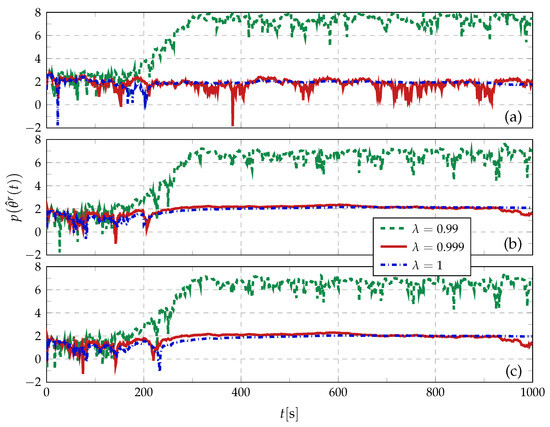
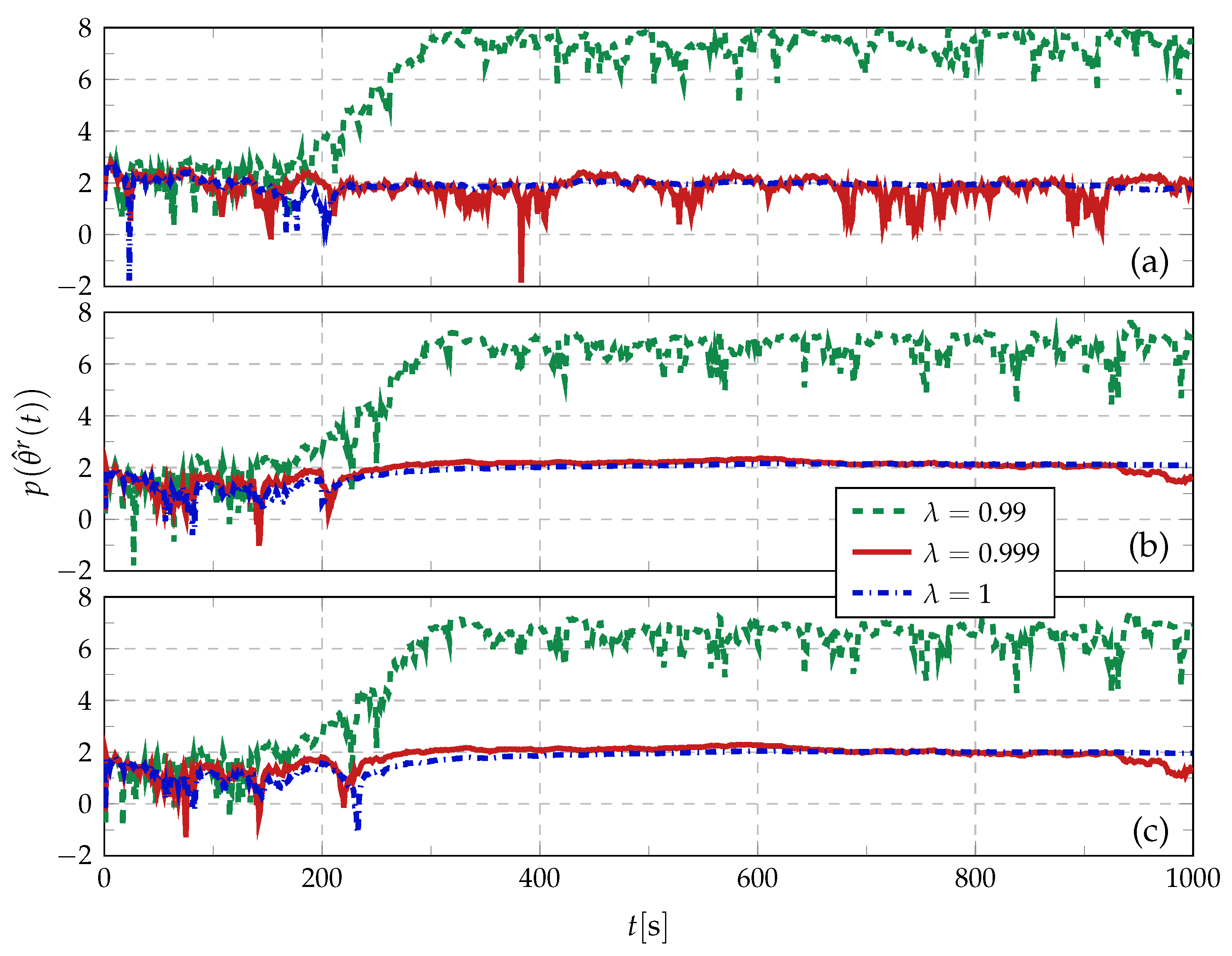
We first simulate a baseline characterized by a non-switching controller fixed at $i=3$ and without resetting the information matrix $E\left(t\right)$. Figure 1 shows the evolution of the estimation error for a selection of parameters in $\widehat{\theta }\left(t\right)$ for three different forgetting factors, and Table 6 shows the variance of the estimated value during the last 200 steps of simulation, which represents a span of time with invariant dynamics.

Figure 1. Time evolution of the estimates ${log}_{10}$ percentage error for a subset of $\widehat{\theta }\left(t\right)$ without switching and without resetting of $E\left(t\right)$: (a) ${\widehat{\theta }}^r\left(t\right)={\widehat{A}}_{12}\left(t\right)$, (b) ${\widehat{\theta }}^r\left(t\right)={\widehat{A}}_{22}\left(t\right)$ and (c) ${\widehat{\theta }}^r\left(t\right)={\widehat{B}}_{21}\left(t\right)$.

Table 6. Variance of the estimates ${log}_{10}$ percentage error for a subset of $\widehat{\theta }\left(t\right)$ without switching and without resetting of $E\left(t\right)$.

	$\mathit{\lambda }=0.99$	$\mathit{\lambda }=0.999$	$\mathit{\lambda }=1$
${\widehat{A}}_{12}\left(t\right)$	$6.11\times {10}^{14}$	$8.92\times {10}^2$	$11.25$
${\widehat{A}}_{22}\left(t\right)$	$0.35\times {10}^{14}$	$0.30\times {10}^2$	$0.16$
${\widehat{B}}_{21}\left(t\right)$	$0.17\times {10}^{14}$	$0.21\times {10}^2$	$0.12$

From Table 6 we observe that an increase in $\lambda$ reduces the variability of the estimates by increasingly averaging the effect of the external perturbation. Nevertheless, the recursive estimation is feed with closed-loop data generated with a single controller, and therefore the estimates are biased, with an estimation error close to 100% in the best scenario (for $\lambda =\left\{0.99,1\right\}$) (cf. Figure 1). Furthermore, notice that the bias of ${\widehat{A}}_{12}\left(t\right)$ is up to 4 orders of magnitude larger than for the other presented parameters, which can be explained by the mass-spring-damper dynamics. Indeed ${\widehat{A}}_{12}\left(t\right)$ represents the effect of velocity over position, which is an internal state transition of the system, while the force input acts directly only over the velocity rate, and therefore their interaction is explicit in the closed-loop data.

5.3. Switching for Informativity

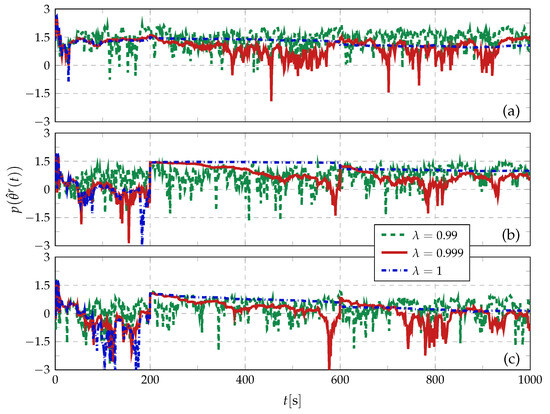
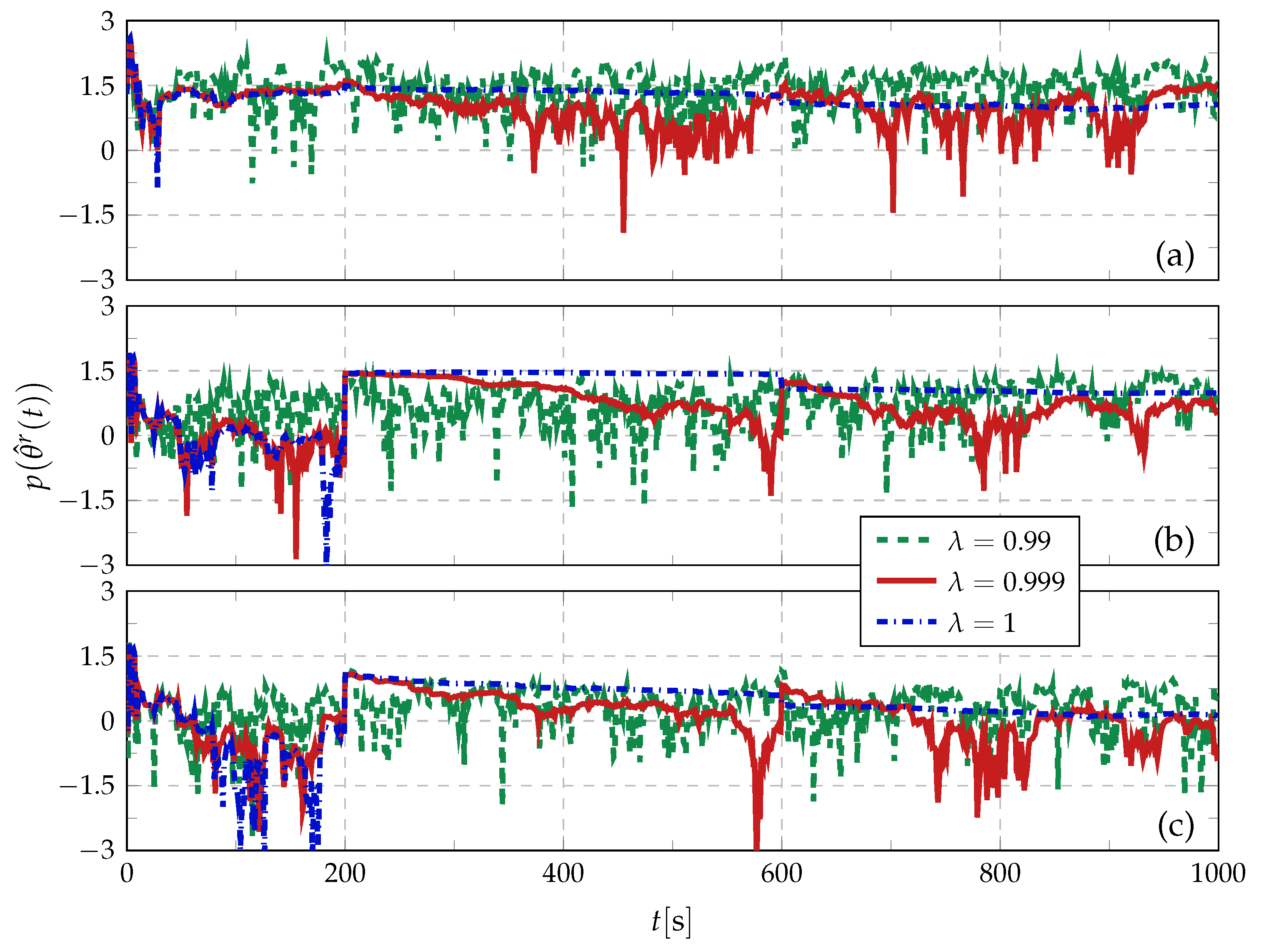
Figure 2 shows the error evolution for all forgetting factors when switching took place according to the selected SSQ and the computed MDTs, yet without resetting the information matrix $E\left(t\right)$. As expected, the RLS with full memory underperform given that it cannot forget the outdated dynamics after variations occur. Oppositely, the case with $\lambda =0.999$ is able to converge to unbiased estimates with errors under 0.1% in some parameters (e.g., ${\widehat{\theta }}^r\left(t\right)={\widehat{A}}_{22}\left(t\right)$)—a result of the SSI condition achieved by switching among controllers according to Corollary 1. Nevertheless, the estimation error with $\lambda =0.99$ does not converge, presenting a variance of 92% even after 300 steps of invariant dynamics, which evidences the need for a low amount of forgetting to address the level of external perturbation ${\mathbb{W}}_e$ of this example.

Figure 2. Time evolution of the estimates ${log}_{10}$ percentage error for a subset of $\widehat{\theta }\left(t\right)$ with switching and without resetting of $E\left(t\right)$: (a) ${\widehat{\theta }}^r\left(t\right)={\widehat{A}}_{12}\left(t\right)$, (b) ${\widehat{\theta }}^r\left(t\right)={\widehat{A}}_{22}\left(t\right)$ and (c) ${\widehat{\theta }}^r\left(t\right)={\widehat{B}}_{21}\left(t\right)$.

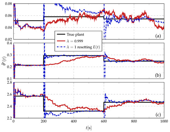
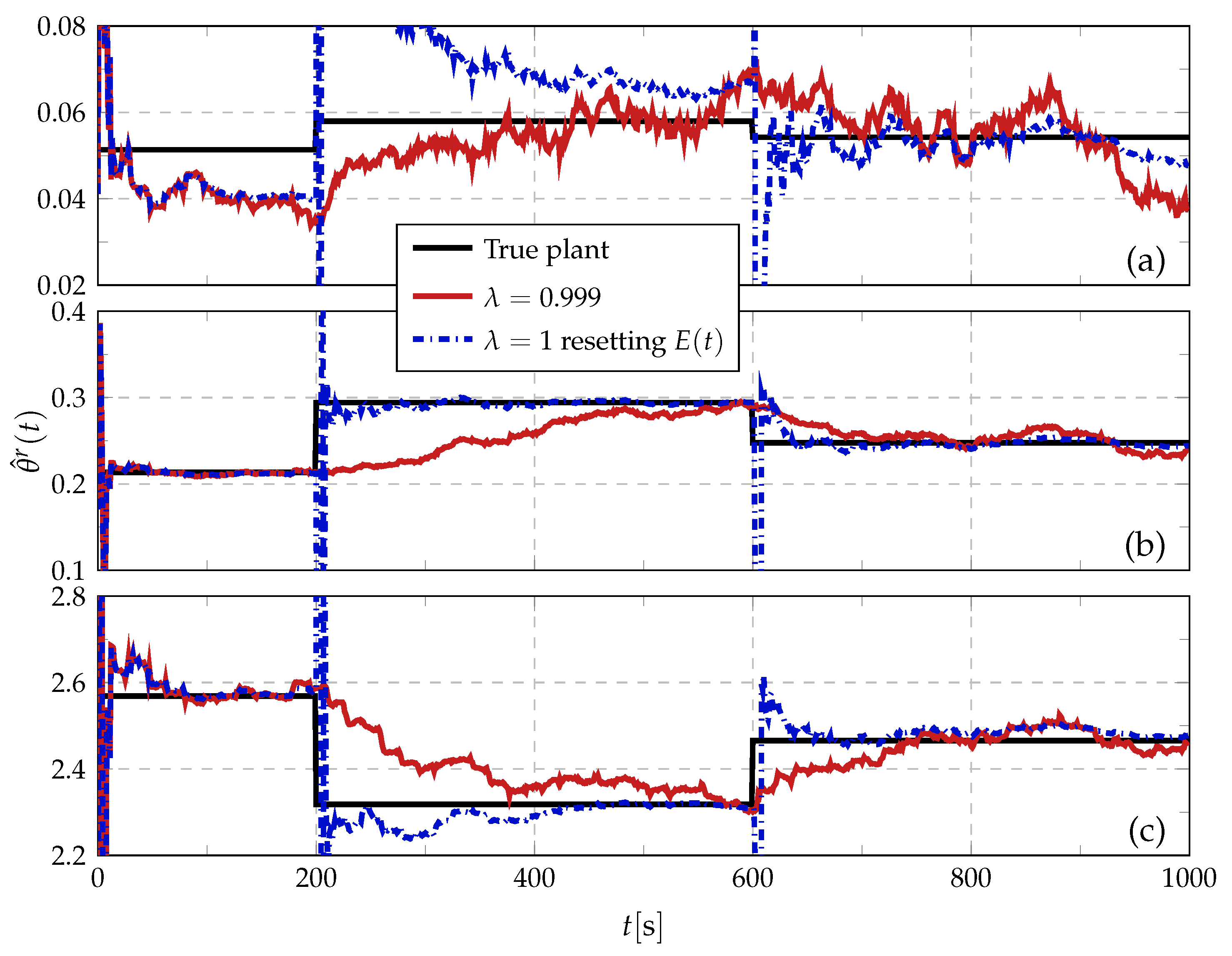
Finally, Figure 3 shows the time evolution of the estimates obtained via switching controllers, with and without resetting of $E\left(t\right)$, for $\lambda =1$ and $\lambda =0.999$ respectively. Again we observe unbiased convergence thanks to the switching, and that resetting the information matrix $E\left(t\right)$ allows for faster convergence of the parameters that interact directly with the input (such as ${\widehat{A}}_{22}\left(t\right)$ and ${\widehat{B}}_{21}\left(t\right)$). For ${\widehat{A}}_{12}\left(t\right)$ we obtain similar convergence rate with and without resetting, which may be a result of the indirect interaction between position and force in the mass-spring-damper system. However, resetting the information matrix allows a selection of $\lambda =1$, improving the filtering capabilities of the RLS and decreasing the variability of the converged estimate error, as depicted in Table 7.

Figure 3. Time evolution of the estimates for a subset of $\widehat{\theta }\left(t\right)$ with switching: (a) ${\widehat{\theta }}^r\left(t\right)={\widehat{A}}_{12}\left(t\right)$, (b) ${\widehat{\theta }}^r\left(t\right)={\widehat{A}}_{22}\left(t\right)$ and (c) ${\widehat{\theta }}^r\left(t\right)={\widehat{B}}_{21}\left(t\right)$.

Table 7. Variance of the estimates ${log}_{10}$ percentage error for a subset of $\widehat{\theta }\left(t\right)$ with switching.

	$\mathit{\lambda }=0.999$ (No Resetting)	$\mathit{\lambda }=1$ (Resetting)
${\widehat{A}}_{12}\left(t\right)$	$5.154$	$0.485$
${\widehat{A}}_{22}\left(t\right)$	$0.890$	$0.040$
${\widehat{B}}_{21}\left(t\right)$	$0.088$	$0.004$

5.4. Closed-Loop Results

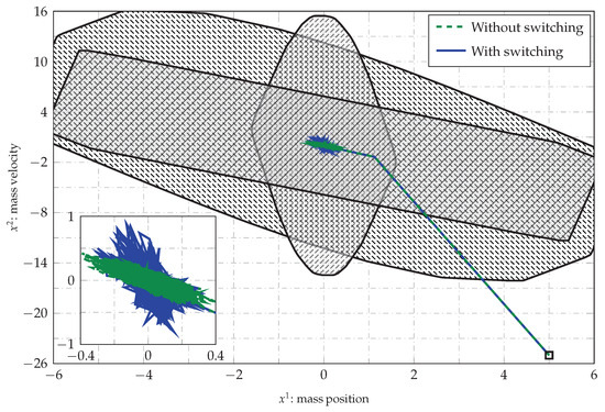
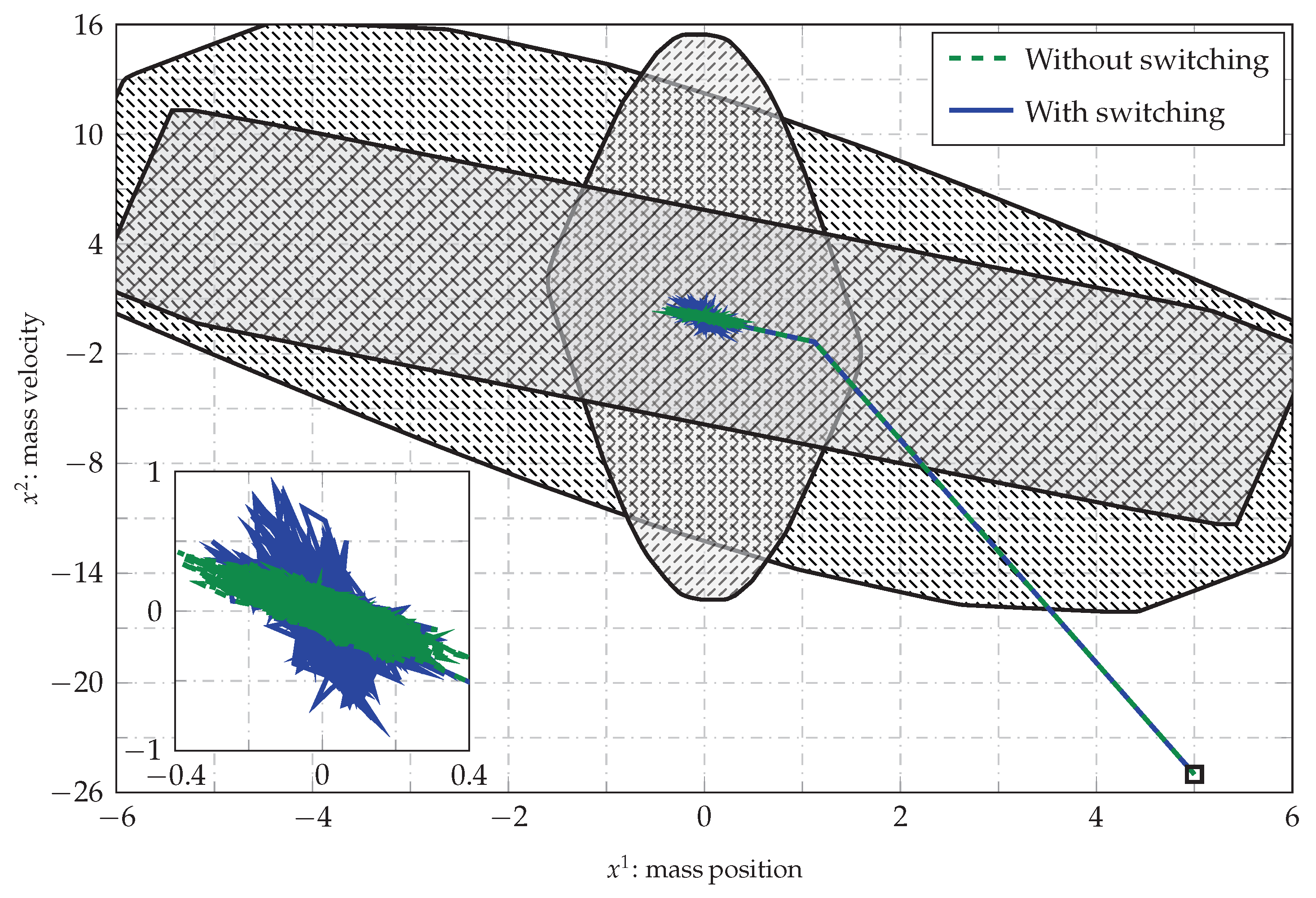
An important requirement of Lemma 1—and of control systems in general—is a stable closed-loop behavior, which is guaranteed by Theorem 1 for our adaptive switching scheme. Figure 4 shows a phase-plot of the state trajectories for $\lambda =1$ with and without switching (fixed at controller $i=3$), where in both cases the trajectories converge to a neighborhood of the origin. Without switching the closed-loop converges to the inside of set ${\mathbb{S}}_3$, while in the switching case to a subset of the intersection of the RPI sets of all modes, as guaranteed by the appropriate computation and enforcement of MDTs. We also observe that, once converged, both trajectories are contained within bounding boxes of similar size. After convergence, the variance in the position is 33% lower when switching took place, while the velocity variance grows only $2.8$ times (see Table 8), which confirms that the unbiased convergence of the estimates is not a result of larger oscillations, but of the informative data guaranteed by the switching control law.

Figure 4. Phase plot of the state trajectories with and without switching: RPI sets ${\mathbb{S}}_1$ , ${\mathbb{S}}_2$ and ${\mathbb{S}}_3$ .

Table 8. Variance of the states trajectories after convergence.

	${\mathit{x}}_1$	${\mathit{x}}_2$
Without switching	$0.018$	$0.020$
With switching	$0.012$	$0.056$

6. Conclusions

In this paper we have shown that a switching MPC architecture with guaranteed stability and constraint satisfaction is able to generate informative data in closed-loop, without the inclusion of purposeful excitation, nor the modification of the standard MPC optimal control problem. The results show that the piece-wise linearity of the control law is not only sufficient, but necessary for the unbiased convergence of the RLS, even in the presence of external uncontrolled disturbances. Moreover, our data matrix reset trigger allows the recursive estimation algorithm to account for confined instances of variation in the the plant, while retaining filtering capabilities. Future work will focus on the implementation of subspace identification methods, to work towards an output tracking framework.

References

- Ma, A.; Li, D.; Xi, Y. Robust tube-based distributed MPC for PWA systems. IET Control Theory Appl. 2023, 17, 2205–2214. [Google Scholar]
- Vicente, B.A.H.; Trodden, P.A. Switching Tube-Based MPC: Characterization of Minimum Dwell-Time for Feasible and Robustly Stable Switching. IEEE Trans. Autom. Control 2019, 64, 4345–4352. [Google Scholar]
- Lin, M.; Ning, Z.; Li, B.; Zhang, K. Adaptive dual model predictive control for linear systems with parametric uncertainties. IET Control Theory Appl. 2022, 16, 1075–1085. [Google Scholar] [CrossRef] [Scilit]
- Zeng, Z.; Wang, H.; Shan, Y. Data-Driven Koopman Operator-Based Model Predictive Control with Adaptive Dictionary Learning for Nonlinear Industrial Process Optimization. Mathematics 2026, 14, 1320. [Google Scholar] [CrossRef] [Scilit]
- Gulewicz, D.; Inyang-Udoh, U.; Bird, T.; Jain, N. Nonlinear Model Predictive Control of a Hybrid Thermal Management System. IEEE Trans. Control Syst. Technol. 2025, 34, 892–905. [Google Scholar] [CrossRef] [Scilit]
- Rawlings, J.B.; Mayne, D.Q.; Diehl, M.M. Model Predictive Control: Theory, Computation and Design, paperback ed.; Nob Hill Publishing: Madison, WI, USA, 2020. [Google Scholar]
- Gao, Y.; Gray, A.; Tseng, H.E.; Borrelli, F. A tube-based robust nonlinear predictive control approach to semiautonomous ground vehicles. Veh. Syst. Dyn. 2014, 52, 802–823. [Google Scholar] [CrossRef] [Scilit]
- Trodden, P. A One-Step Approach to Computing a Polytopic Robust Positively Invariant Set. IEEE Trans. Autom. Control 2016, 61, 4100–4105. [Google Scholar] [CrossRef] [Scilit]
- Adetola, V.; DeHaan, D.; Guay, M. Adaptive model predictive control for constrained nonlinear systems. Syst. Control Lett. 2009, 58, 320–326. [Google Scholar] [CrossRef] [Scilit]
- Gonçalves, G.A.; Guay, M. Robust discrete-time set-based adaptive predictive control for nonlinear systems. J. Process Control 2016, 39, 111–122. [Google Scholar] [CrossRef] [Scilit]
- Lorenzen, M.; Cannon, M.; Allgöwer, F. Robust MPC with recursive model update. Automatica 2019, 103, 461–471. [Google Scholar] [CrossRef] [Scilit]
- Anderson, A.; González, A.; Ferramosca, A.; D’Jorge, A.; Kofman, E. Robust MPC suitable for closed-loop re-identification, based on probabilistic invariant sets. Syst. Control Lett. 2018, 118, 84–93. [Google Scholar]
- Heirung, T.A.N.; Ydstie, B.E.; Foss, B. Dual adaptive model predictive control. Automatica 2017, 80, 340–348. [Google Scholar] [CrossRef] [Scilit]
- Larsson, C.A.; Rojas, C.R.; Bombois, X.; Hjalmarsson, H. Experimental evaluation of model predictive control with excitation (MPC-X) on an industrial depropanizer. J. Process Control 2015, 31, 1–16. [Google Scholar] [CrossRef] [Scilit]
- Green, M.; Moore, J.B. Persistence of excitation in linear systems. Syst. Control Lett. 1986, 7, 351–360. [Google Scholar] [CrossRef] [Scilit]
- Ljung, L. System Identification Theory for the User, 2nd ed.; Prentice Hall: Upper Saddle River, NJ, USA, 1998; p. 640. [Google Scholar]
- Genceli, H.; Nikolaou, M. New approach to constrained predictive control with simultaneous model identification. AIChE J. 1996, 42, 2857–2868. [Google Scholar] [CrossRef] [Scilit]
- Lu, X.; Cannon, M.; Koksal-Rivet, D. Robust adaptive model predictive control: Performance and parameter estimation. Int. J. Robust Nonlinear Control 2021, 31, 8703–8724. [Google Scholar]
- Lu, X.; Cannon, M. Robust adaptive model predictive control with persistent excitation conditions. Automatica 2023, 152, 110959. [Google Scholar] [CrossRef] [Scilit]
- Hernandez Vicente, B.A. Eigenvalue Characterization of Persistence of Excitation for Convex Adaptive Predictive Control. Int. J. Adapt. Control Signal Process. 2026, 1–11. [Google Scholar]
- Vicente, B.A.H.; Trodden, P.A. Stabilizing predictive control with persistence of excitation for constrained linear systems. Syst. Control Lett. 2019, 126, 58–66. [Google Scholar] [CrossRef] [Scilit]
- Zhu, Y.; Yan, W.; Zhu, Y. MPC closed-loop identification without excitation. J. Process Control 2021, 106, 122–129. [Google Scholar] [CrossRef] [Scilit]
- Soderstrom, T.; Ljung, L.; Gustavsson, I. Identifiability conditions for linear multivariable systems operating under feedback. IEEE Trans. Autom. Control 1976, 21, 837–840. [Google Scholar] [CrossRef]
- Shorten, R.; Wirth, F.; Mason, O.; Wulff, K.; King, C. Stability Criteria for Switched and Hybrid Systems. SIAM Rev. 2007, 49, 545–592. [Google Scholar] [CrossRef] [Scilit]
- Ong, C.J.; Wang, Z.; Dehghan, M. Model Predictive Control for Switching Systems With Dwell-Time Restriction. IEEE Trans. Autom. Control 2016, 61, 4189–4195. [Google Scholar] [CrossRef] [Scilit]
- Dehghan, M.; Ong, C.J. Discrete-time switching linear system with constraints: Characterization and computation of invariant sets under dwell-time consideration. Automatica 2012, 48, 964–969. [Google Scholar] [CrossRef] [Scilit]
- Bridgeman, L.J.; Danielson, C.; Di Cairano, S. Stability and feasibility of MPC for switched linear systems with dwell-time constraints. In Proceedings of the 2016 American Control Conference (ACC), Boston, MA, USA, 6–8 July 2016; pp. 2681–2686. [Google Scholar]
- Zhang, L.; Zhuang, S.; Braatz, R.D. Switched model predictive control of switched linear systems: Feasibility, stability and robustness. Automatica 2016, 67, 8–21. [Google Scholar] [CrossRef] [Scilit]
- Ljung, L.; Gustavsson, I.; Soderstrom, T. Identification of linear, multivariable systems operating under linear feedback control. IEEE Trans. Autom. Control 1974, 19, 836–840. [Google Scholar] [CrossRef]
- Mayne, D.Q.; Seron, M.M.; Raković, S.V. Robust model predictive control of constrained linear systems with bounded disturbances. Automatica 2005, 41, 219–224. [Google Scholar] [CrossRef] [Scilit]
- Hansen, P.C. Rank-Deficient and Discrete Ill-Posed Problems: Numerical Aspects of Linear Inversion; Mathematical Modeling and Computation; Society for Industrial and Applied Mathematics (SIAM): Philadelphia, PA, USA, 1998; Volume 4. [Google Scholar]
- Kolmanovsky, I.; Gilbert, E.G. Theory and computation of disturbance invariant sets for discrete-time linear systems. Math. Probl. Eng. 1998, 4, 934097. [Google Scholar] [CrossRef] [Scilit]
Disclaimer/Publisher’s Note: The statements, opinions and data contained in all publications are solely those of the individual author(s) and contributor(s) and not of MDPI and/or the editor(s). MDPI and/or the editor(s) disclaim responsibility for any injury to people or property resulting from any ideas, methods, instructions or products referred to in the content. |
© 2026 by the authors. Licensee MDPI, Basel, Switzerland. This article is an open access article distributed under the terms and conditions of the Creative Commons Attribution (CC BY) license.